Guest essay by Joe Born
In a recent post Christopher Monckton identified me as a proponent of the following proposition: The observed decay of bomb-generated atmospheric-carbon-14 concentration does not tell us how fast elevated atmospheric carbon-dioxide levels would subside if we discontinued the elevated emissions that are causing them. He was entirely justified in doing so; I had gone out of my way to bring that argument to his attention.
But I was merely passing along an argument to which a previous WUWT post had alerted me, and the truth is that I’m not at all sure what the answer is. Moreover, semantic issues diverted the ensuing discussion from what Lord Monckton probably intended to elicit. So, at least in my view, we failed to join issue.
In this post I will attempt to remedy that failure by explaining the weakness that afflicts the position attributed (again, understandably) to me. I hasten to add that I don’t profess to have the answer, so be forewarned that no conclusion lies at the end of this post. But I do hope to make clearer where at least this layman thinks the real questions lie.

To start off, let’s review the argument I made, which is that the atmospheric-carbon-dioxide turnover time is what determined how long the post-bomb-test excess-carbon-14 level took to decay. That argument was based on the “bathtub” model, which Fig. 1 depicts. The rate at which the quantity <i>m</i> of water the tub contains changes is equal to the difference between the respective rates <i>e</i> (emissions) and <i>u</i> (uptake) at which water enters from a faucet and leaves through a drain:

The same thing can, <i>mutatis mutandis</i>, be said of contaminants (read carbon-14) in the water. But in the case of well-mixed contaminants one of the <i>mutanda</i> is that the rate at which the contaminants leave is dictated by the rate at which water leaves:

where 

Consequently, if the water quantity increases for an interval during which <i>e</i> exceeds <i>u</i>, it will thereafter remain elevated if the emissions rate <i>e</i> then falls no lower than the drain rate <i>u</i>. If a dose of contaminants is added to the water, though, the resultant contaminant amount falls, even when there’s no difference between <i>u</i> and <i>e</i>, in accordance with the <i>turnover</i> rate, i.e., with the ratio of <i>u</i> to <i>m</i>. So, to the extent that this model reflects reality’s relevant aspects, we can conclude that the rate at which the carbon-14 concentration decays tells us nothing about what happens when total-CO2 emissions return to a “normal” level.
But among the foregoing model’s deficiencies is that it says nothing about a possible dependence of overall drain rate <i>u</i> on the water quantity <i>m</i>, whereas we may expect biosphere uptake (and emissions) to respond to the atmosphere’s carbon-dioxide content. Nor does it deal with the possibility that after contamination has flowed out the drain it will be recycled through the faucet. In contrast, the biosphere no doubt returns to the atmosphere at least some of the carbon-14 it has previously taken from it.

A model that takes such factors into account could support a conclusion different from the one to which the bathtub led us. Consistently with my last post’s approach, Fig. 2 uses interconnected pressure vessels to represent one such model. In this case there are only two vessels, the left one representing the atmosphere and the right one representing carbon sinks such as the ocean and the biosphere.
The vessels contain respective quantities 


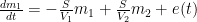
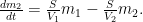
Those equations tell us that the carbon quantity 
![m_1(t) = \left[ \frac{V_1}{V_1+V_2}+\frac{V_2}{V_1+V_2} \exp\left(-\frac{V_1+V_2}{V_1V_2}St \right)\right] m_0 ,](https://s0.wp.com/latex.php?latex=m_1%28t%29+%3D+%5Cleft%5B+%5Cfrac%7BV_1%7D%7BV_1%2BV_2%7D%2B%5Cfrac%7BV_2%7D%7BV_1%2BV_2%7D+%5Cexp%5Cleft%28-%5Cfrac%7BV_1%2BV_2%7D%7BV_1V_2%7DSt+%5Cright%29%5Cright%5D+m_0+%2C+&bg=ffffff&fg=000&s=0&c=20201002)
which the substitutions 

Note that in the Fig. 2 system any constituent of the gas would be exchanged between vessels in accordance with the partial-pressure difference of that constituent alone, as if it were the only component the vessels contained. By thus constraining the flow from (and to) the first, atmosphere-representing vessel, this model supports the conclusion that the overall-carbon-dioxide quantity would, contrary to my previous argument, decay just as the excess, bomb-caused quantity of atmospheric carbon-14 did.

Could providing more than one sink enable us to escape that conclusion? Not necessarily. Consider the more-complex system that Fig. 3 depicts. Just as the system that my previous post described, this one can embody the TAR Bern-model parameters. As that post indicated, describing such a system requires a fourth-order linear differential equation. So that system does have more degrees of freedom in its initial conditions and can therefore exhibit a wider range of responses.
But it still constrains the flow among its four vessels linearly in accordance with partial pressures, just as the Fig. 2 system does. From complete equilibrium, therefore, its behavior for any constituent is the same as for any other constituent as well as for the contents as a whole. In other words, this model, too, seems to support the notion that the bomb-test results do indeed tell us how long excess carbon dioxide will remain if we stop taking advantage of fossil fuels.
In a sense, though, the models of Figs. 2 and 3 beg the question; they use the same uptake- and emissions-process-representing
So one question is how significant that difference is in the present context. I don’t have the answer, although my guess is, not very. But readers attempting to answer that question could do worse than start by referring to a previous WUWT post by Ferdinand Engelbeen.

Another way in which carbon-14 differs from the other two carbon isotopes is that it’s unstable. So, if the Fig. 3 model is adequate for carbon-12 or -13, a different model, which Fig. 4 depicts, would have to be used for carbon-14 if its radioactive decay is significant. That diagram differs from Fig. 3 in that it includes a flow 
To the extent that those different models produce different responses, using bomb-test data to predict the total carbon content’s behavior is problematic. But the Engelbeen post mentioned above seems to say that even deep-ocean residence times tend to be only a minor fraction of carbon-14’s half-life: this factor’s impact may be small.
A possibly more-significant factor is that the carbon cycle is undoubtedly non-linear, whereas the conclusions we tentatively drew from the models above depend greatly on their linearity. Before I reach that issue, though, I should point out an aspect of the Bern model that was not relevant to my previous post. The Bern equations I set forth in my last post were indeed linear. But that does not mean that their authors meant to say that the carbon cycle itself is. Although for the sake of simplicity I’ve discussed the models’ physical quantities as though they represented, e.g., the entire mass of carbon in a reservoir, their authors no doubt intended their (linear) models’ quantities to represent only the differences from some base, pre-industrial values. Presumably the purpose was to limit their range enough that the corresponding real-world behavior would approximate linearity.
But such linearization compromises the conclusions to which the models of Figs. 2 and 3 led us. A linear system is distinguished by the fact that its response to a composite stimulus always equals the sum of its individual responses to the stimulus’s various constituents; if the stimulus equals the sum of a step and a sine wave, for example, the system’s response to that stimulus will equal the sum of what its respective responses would have been to separate applications of the step and the sine wave. And this “superposition” property was central to drawing the conclusions we did from those models: the response to a large stimulus is proportionately the same as the response to a small one.

To appreciate this, consider Fig. 5, which depicts scaled values of the Fig. 2 model’s left-vessel total-carbon and carbon-14 contents. Initially, the system is at equilibrium, with zero outside emissions 


At time t = 5, a bolus of carbon-14 appears in the (atmosphere-representing) left vessel. Compared with the total carbon content, the added quantity is tiny, but it is large enough to double the small existing carbon-14 content. As the distance between the red dotted vertical lines shows, the resultant increase in carbon-14 content decays toward its new equilibrium value with a time constant of just about seven years. (I’ve assumed that the processes greatly favor the sink-representing right vessel—i.e., that its “volume” is much greater than the left vessel’s—so that the new equilibrium value is not much greater than the original.)
Now consider what happens at t = 45, when the left vessel’s total-carbon quantity suddenly increases. Although the two quantities are scaled to their respective initial values, this total-carbon increase is orders of magnitude greater than the t = 5 carbon-14 increase. Yet, as the black dotted vertical lines show, the decay of the left vessel’s total-carbon content proceeds just as fast proportionately as the much-smaller carbon-14 content did. As was observed above, this could tempt one to conclude that the carbon-14 decay we’ve observed in the real world tells us how fast the atmosphere would respond to our discontinuing fossil-fuel use.
![clip_image009[1]](http://wattsupwiththat.files.wordpress.com/2013/12/clip_image0091.png?quality=75 "clip_image009[1]")
But now consider what can happen if we relax the linearity assumption. Specifically, let’s say that the Fig. 2 model’s proportionality “constant”

In that plot, the red lines show that the carbon-14 decay occurs just as fast as in the previous plot, the carbon-14 content falling to exp(-1) above its new equilibrium value in around seven years. But the much-larger total-carbon increase brings the system into a lower-efficiency range, so that quantity subsides at a more-leisurely pace, taking over forty years. If such results are any indication, bomb-test results are a poor predictor of how long total-carbon content will settle.
Now permit me a digression in which I attempt to forestall pointless discussion of precisely what the quantities are that the graphs show. I believe the exposition is clearest if it is directed, as in Figs. 5 and 6, to ratios that carbon 14 and total carbon bear to their own initial values. But it appears customary to express the carbon-14 content instead in terms of its ratio to total carbon content. This means that, since total carbon has been increasing, the numbers commonly used in carbon-14 discussions could fall below the pre-bomb values, even though total carbon-14 has in fact increased.
For the sake of those to whom that issue looms large, I have attached Fig. 7 to illustrate how the values for carbon-14 itself could differ from those of its ratio to total carbon in a situation in which new (carbon-14-depleted) carbon is continually injected into the atmosphere.

But that’s a detail. More important is the issue that Fig. 6 raises.
Now, I “cooked” Fig. 6’s numbers to emphasize the point that nonlinearity can undermine conclusions based on linear models. Specifically, Fig. 6 depicts the results of making the flows proportional only to the fifth root of the carbon content.
But non-linearity must have some effect. How much? I don’t know. Together with the differences in behavior between carbon-14 and its stable siblings, though, it is among the considerations to take into account in assessing how informative the bomb-test data are.
As I warned at the top of the post, this post draws no conclusions from these considerations. But maybe the foregoing analysis will prompt knowledgeable readers’ comments that help narrow the issues.
Discover more from Watts Up With That?
Subscribe to get the latest posts sent to your email.
I have seen the point made hundreds of times that the residence time of an average molecule is different than the time for a pulse to decay back to equilibrium. Usually this point is made in pedantic fashion, as if it were a tiresome chore to explain such a simple point to such simpletons. But I still don’t get it. Are the molecules in the pulse exempt from the processes giving rise to the properties of the residence time of average molecules? Are they not average molecules? How so? What qualifies a molecule, or group of molecules, to be treated as part of a slug or pulse on the one hand that is governed by pulse decay rules or merely part of the background sources of emissions governed by residence time of average molecule rules? How do it know? Where human emissions are a single digit percentage of natural emissions, which source is the slug? What is the threshold at which or the rules by which emissions from one or the other, human or natural, transition from being subject to average molecule processes to slug molecule processes? How do it know?
Ferdinand Engelbeen: “40.5 GtC out of the atmosphere into the deep oceans, 39.5 GtC into the atmosphere, caused by the extra pressure from the 100 GtC increase of CO2 in the atmosphere. That is for 100% CO2 out into the deep, 97.5% is coming back from the deep oceans.”
Thanks a lot for that response; it answers my question nicely.
If I can again abuse your patience, what are K and k in your diagrams? I couldn’t readily find the accompanying text on your site.
Ferdinand Englebeen: “From the 100% 14CO2 spike going into the deep (1960), 97.5% (as mass) * 45% (as concentration) is coming back, that is only 42.8% is coming back from the deep oceans.” Is this the loss of that spike since 1960 or is it a suggestion that the kinetic difference between 14C and 12C is that large? I couldn’t quickly find kinetic differences for carbon isotopes but would be surprised if they are that large. I’d also expect the kinetic differences to be process dependent.
Bernie Hutchins “This is NOT to suggest that the electrical equivalents could not be completely correct and very useful as models for CO2 migrations. The mathematics (that is – the physics) is very similar if not identical.”
For the linear models above, RC-circuit mathematics is indeed identical. But using a signed quantity (charge) to represent an unsigned quantity (mass) can lead to some conceptual confusion. Although the left vessel is connected in series between the source and the right vessel, for example, the analog’s current source would have to be wired in parallel with the capacitor representing the left vessel and with the RC-series combination representing the right vessel and its flow restriction.
I assume all the discussion of CO2 mass balance is based on the assumption that the CO2 distribution in the atmosphere is homogeneous and can be represented by one measuring location. Other things, liquid or gas, require relatively great amounts of energy to get homogeneous mixtures at much lower volumes. Is the atmospheric CO2 that homogeneous and if not, how much does that affect these estimates?
Bob Greene: “Is the atmospheric CO2 that homogeneous and if not, how much does that affect these estimates?”
Someone has probably already answered this question somewhere, but I haven’t found it yet myself. I’ve wondered whether the “missing sink” may be a reflection of greatly enhanced uptake at areas of locally intense near-power-plant (or -highway) concentrations not reflected in the more-general CO2 numbers we see–uptake that is not offset substantially by locally enhanced natural emissions.
No doubt a naive notion that has already been laid to rest elsewhere, but it’s one of which I haven’t yet been disabused.
Quinn the Eskimo says:
December 12, 2013 at 4:07 am
I have seen the point made hundreds of times that the residence time of an average molecule is different than the time for a pulse to decay back to equilibrium.
I know, this seems to be one of the most difficult points to be explained…
The simplest way is to describe it as the difference between the turnover of capital (thus goods) in a factory and the gain or loss that that capital makes (over a year).
The turnover gives how much times a capital is going through the factory: from the purchase of raw materials to the sales of the endproduct.
The yield of the factory is what is gained or lost of its capital after the turnover(s).
Both are about the same money, but they are largely independent of each other: you can double the turnover, but that may or may not increase the gain, because you have to pay higher wages for overtime, or you may get from a loss to a gain…
The same for 14CO2 vs. 12CO2:
With the 14CO2 bomb spike, you are mostly measuring the turnover of CO2 through the atmosphere, without influencing the mass (total capital).
With a 12CO2 spike, you are increasing the total mass (capital), whithout influencing the turnover that much: the turnover will be somewhat diluted (more in the atmosphere, about the same througput).
The decay rate of an excess mass of 12CO2 depends of how fast the deep oceans (less for other reservoirs) take an extra mass of CO2 away from the atmosphere (partial pressure difference related), while the decay rate of an excess concentration of 14CO2 depends of the turnover (which is temperature difference related, mostly between equator and poles)…
Monckton of Brenchley says:
December 12, 2013 at 12:51 am
Why is half of all the CO2 we emit disappearing instantaneously from the atmosphere?
============
This does appear to be the nub of the problem. Why does this number remain at 1/2 of human emissions, rather than a fraction of cumulative CO2 excess?
If we consider the bathtub model, then the amount flowing out remains at 1/2 the amount flowing in, regardless of the height of water in the tub. Which makes no sense. The amount flowing out should vary as the height of water in the tub, not as the amount flowing in.
Which argues that the bathtub model does not describe CO2 reality.
Joe Born says:
December 12, 2013 at 4:16 am
If I can again abuse your patience, what are K and k in your diagrams? I couldn’t readily find the accompanying text on your site.
You are welcome…
K and k should all be k and are the rate constants for all transfers, where I should switch the +’s and -‘s, as normally one looks at the atmosphere as starting and end place…
Still to be worked out, as good as the whole page I need to devote to the explanation of all these diagrams and a lot more…
The methane residency time is also likely much lower than currently believed. As we discover more and more sources, we must realize that there more sinks or that sinks respond to emissions to keep methane levels from growing much.
ferd berple says:
December 12, 2013 at 4:47 am
This does appear to be the nub of the problem. Why does this number remain at 1/2 of human emissions, rather than a fraction of cumulative CO2 excess?
In fact it is pure coincidence: human emissions increased slightly quadratic over time, which gives a slightly quadratic increase of the residuals in the atmosphere (= pressure) and which causes a slightly quadratic increase in sink rate. The result is an astonishing fixed ratio between emissions and increase in the atmosphere (the “airborne fraction”):
http://www.ferdinand-engelbeen.be/klimaat/klim_img/temp_co2_acc_1960_cur.jpg
or in ratio since 1900:
http://www.ferdinand-engelbeen.be/klimaat/klim_img/acc_co2_1900_cur.jpg
or since 1960:
http://www.ferdinand-engelbeen.be/klimaat/klim_img/acc_co2_1960_cur.jpg
where the South Pole (SPO) lags the Mauna Loa (MLO) data.
If the human emissions would stay the same, the “airborne fraction” would decrease and CO2 levels would go assymptotically to a new steady state equilibrium CO2 level…
Hoser says:
December 11, 2013 at 11:32 pm
Hopelessly over complicated.
—————————
Indeed. All this analysis of 1 part of 20,000 parts of the atmosphere changing from “something” to CO2. A change of .005%, while the other 99.995% purportedly has been expected to remain stable and have influence. Oh the effort that has been spent on solving a puzzle that is simply a figment of someone’s overactive imagination.
Bob Greene says:
December 12, 2013 at 4:29 am
I assume all the discussion of CO2 mass balance is based on the assumption that the CO2 distribution in the atmosphere is homogeneous and can be represented by one measuring location.
For most of the atmosphere, the CO2 levels are within +/- 2% of full scale, despite that some 20% of all CO2 in the atmosphere is exchanged with CO2 of other reservoirs each year. Seems to be quite nicely and fast mixed. There are lags between near-ground and height and between the NH and the SH. The largest differences are in the first few hundred meters over land, where the largest/fastest sources and sinks are at work.
But have a look at what different stations find:
http://www.esrl.noaa.gov/gmd/dv/iadv/
Thus while there are huge CO2 level differences around vegetation (day/night difference of several hundred ppmv!), that doesn’t exist for the air over the oceans, where the 14C/12C decay rates have the highest difference in decay rate…
It also means there’s a good bit of fossil carbon in the atmosphere from natural sources.
I take no joy in this, but the fallacies are so deep that it warrants no less than a full fisking of Ferdinand:
” 50% bomb spike level goes into the deep oceans, 45% comes out after ~1000 years,”
Maxwell called and said he wanted his demon back. Putting aside gedankens of nonsense, it is wholly irrelevant to the topic at hand: The bomb spikes that happened ~50 years ago. Perhaps the argument can be salvaged with clarity, and perhaps it would be worthwhile to do so if we were discussing some other subject.
“That caused an imbalance between atmosphere and deep oceans where inputs and outputs aren’t equal anymore. ”
The ice core records show that ‘aren’t equal anymore‘ places ‘anymore’ prior to the ice core records themselves. There has never been a proper equality. This is confused and nonresponsive at best, and an attempt at sophistical obfuscation at worst.
“40.5 GtC out of the atmosphere into the deep oceans, 39.5 GtC into the atmosphere, caused by the extra pressure from the 100 GtC increase of CO2 in the atmosphere. ”
Based on what measurements? This is first-order circular nonsense. As it presumes the rates to exist — without any measurements taken — on the basis of global average temperatures as compared to salinity and etc. The 14CO2 discussion is precisely about discarding this vulgar fallacy and making use of actual observations — for good or ill. One cannot ‘prove’ your conclusion by assuming it as a premise. Again, a thoroughly confused point at best, or a sophistry at worst.
“The difference in 12CO2 concentration between ins and outs (both ~99%) is negligible.
Not so for 13CO2 and 14CO2.”
With respect to 14C there is the issue of the radioactive decay that would occur with or without Maxwell’s lesser demon of oceanic circulation. But it was already stated in the same post that: in pre-industrial times there was a balance between decay and production of 14CO2:
Whatever the case may be with radioactive decay is meaningless here. For there was, and ppresumptively is, the same process extant. To the degree there is not that can be haggled over. But tagging a herd of Carbon Dioxide with radioactive tracers isn’t going to upset this long running process that has been stated to be balanced. Again, deep confusion or sophistry.
With respect to isotopic fixation in organisms, it only needs noted that 12C is preferred. So we would see
more 12C sequestered — versus exchanged — than 13C and 14C. That is, the decay curve in the bomb spike represents an upper bound on time for the process in question. But this has precisely nothing to do with the thrust of the ‘ins and outs’ statement or the statements about 14C and CH4.
“The difference between a 12CO2 spike and a 14CO2 spike is caused by the long delay between what goes into the oceans and what comes out, which makes that the 14CO2 (and 13CO2) input is effectively decoupled from the output, while that is hardly the case for 12CO2.”
This is again an instance of Maxwell’s demon. But the difference is between a bolus of CO2 — of any and all isotopes — and radioactively tagging a set of the existing bolus. And to be sure, the idea that there is an increasing ppm of atmospheric CO2 is the entire argument of AGW. That there is a constant excess above equilibrium injected into the atmospheric reservoir. So yes, they are different creatures. One is a bolus without remark, as a pure gedanken, and the other is the actual physical process the gedanken represents — just with extra tagging of the molecules. No more nor less.
So the 13 and 14 CO2 are only decoupled from the output in the same manner that the pedestrian evil of 12CO2 is decoupled. Which is: They aren’t. Perhaps in the purely fictional land of idealized models that have no application outside of validation with measurement. But, once more, this entire discussion is about the rare sighting of a wild observation. A practically mythical beast long thought to be extinct.
Lastly, and out of order from the rest: “From the 100% 14CO2 spike going into the deep (1960), 97.5% (as mass) * 45% (as concentration) is coming back, that is only 42.8% is coming back from the deep oceans.”
Sadly, this one is full of confusion and/or sophistry again. There is again the circular argument based on the models proving the models. There is again, the idea that theory trumps measurement. There is again the special pleading about the deep oceans. The only relevant part to this is that the exchange does matter. And is the entire point behind looking at the bomb test curve in the first place. As given the increasing ppm of CO2, it is not a question that more CO2 is entering the atmosphere than leaving it. And the 14CO2 decay curve gives us an idea of the net flow on the basis of that decay.
There is a lot of heel digging on this issue for no good reason, as the math is entirely straight forward for it. We know the 14CO2 production rate, the (Bomb14)CO2 decay rate, and the historical levels — and so the partial pressure of the atmospheric reservoir of 14CO2; if you’re into bathtub models. Everything is right there to gain the answer.
It is, of course, wholly optional. As we can also get the same sanity check on CO2 cycling by looking at the unsmoothed data from Mauna Loa and other measuring sites. As every summer season the CO2 levels fair plummet. To the degree we add man’s culpability, and have a good measure of how much CO2 that dire beast is putting in the atmostphere, then the rest can be figured out independently from there as well.
That’s two — count them, two — independent sources of actual measurement that can be used to ground the entire discussion in science. The utter allergy to approaching the simple math for either of these is wholly incomprehensible. But Ferdinand deserves a round of applause for suffocating his straw man under a heap of errors.
Ferdinand Engelbeen says:
December 12, 2013 at 5:07 am
In fact it is pure coincidence: …. The result is an astonishing fixed ratio between emissions and increase in the atmosphere
==============
As I explained to the police, it was pure co-incidence my gun was smoking when the victim dropped dead.
What if we make the other assumption, that it is not co-incidence? Does this have implications for the choice of model? If the ratio is not due to co-incidence, but rather the nature of the system, how would this change the model?
phlogiston says:
December 12, 2013 at 12:53 am
It is COMPLETELY IRRELEVANT all the other cycling and dilution and dynamics, pressure, temperature etc. of CO2 that are going on, the 14 tracer simply tells us the removal term for CO2. That is the whole point of a radiotracer measurement.
———————————————————
Amen to that, and no amount of mental masturbation can change it.
This math(s) is virtually identical to that used by pharmacologists/pharmacokineticists for calculating drug dosage in animal models and human studies and treatment. They get it wrong, people die.
Typically, the drug is considered to be, for all intents and purposes, gone at six half-lives, explaining approximately, by analogy, Lindzen’s number (40 years) mentioned in Lord Monckton’s post above.
What reemerges from the sinks, and why is a separate discussion from this. This is the experimentally observed removal term which anyone can see from eyeballing the bomb data is a half-life of 5 or so years.
Ferdinand,
You have the patience of a saint, but are you really making progress? There are none so blind as those who refuse to see.
An elegant mathematical exploration of the travels of our most talked about substance. However indeed,
“Maybe various sinks saturate or become less efficient with increased concentration.”
So far, only the gas guys have responded. CO2 is also a complex chemical, forming carbonic acid in the atmosphere with rain and in its solution into the ocean. Once in the water the acid dissociates into three species:
CO2 +;H2O => H2CO3 => H^+ + HCO3^- => 2nd H^+ + CO3^-2
Now in seawater we have Ca^++ (and other cations which reacts which forms both inorganic limestone precipitate and biologically produced CaCO3 in shells (possibly through the bicarbonate stage), etc. This is sequestered CO2. Also, probably C14 is probably taken up by algae, plankton and the like, similar to the absorption by land plants. Go for the model where the sinks INCREASE their intake by sequestration.
ferd berple says:
December 12, 2013 at 5:43 am
If the ratio is not due to co-incidence, but rather the nature of the system, how would this change the model?
The “model” in this case is the most simple form of reaction: the sink rate of CO2 is directly proportional to the increase in the atmosphere above the (temperature controlled) equilibrium…
Oh my! I remember the hours spent learning to produce qualitatively effective curves of individual isotope activities in a closely empirically engineered system, a nuclear reactor. To attempt the same in an open system is amazing and beyond my ken. I knew that my curves were merely CARTOONS of reality.
Gary Pearse says:
December 12, 2013 at 5:47 am
Go for the model where the sinks INCREASE their intake by sequestration.
==========
In such a bathtub, the drain gets bigger as you increase the input flow. The output is no longer coupled to the height of the bath, rather to the inflow rate.
So, in such a model we have a reverse of the co-incidence proposed above. It is the cumulative excess that is the co-incidence, and the inflow rate that is the determining factor in the outflow.
Such a model may in fact be more likely than the standard bathtub model because the water in a bathtub is not in short supply. But in nature there is ample evidence that CO2 is barely above the minimum required by plants to maintain photosynthesis. As we add CO2 the drain (life) is increasing in size.
In this case it would not be partial pressure that is steering the good ship CO2, rather it is life.
Your figure 4 is essentially right from a simplest box model approach; with V1 atmosphere, V2 terrestrial biomass, V3 the ocean SURFACE and V4 the depths.
Please do not use the word SINK when you mean reservoir, a sink in local or process that is infinite, a kinetic black hole where there is, on the time scale analyzed, zero back rate. In your figure 4 you include a true sink out of V4, the mineralization of carbon.
Now mechanistically we know that the atmosphere. V1, can ‘talk’ to the ocean surface, V3, but cannot ‘talk’ to the deep ocean, V4.
Let us take what we know we know:-
The disappearance of 14CO2 from the atmosphere is first order all the way from the 70’s with a t1/2 of approx 12.5 years.
The disappearance of 14CO2 from the atmosphere has a projected endpoint very near to the pre-1945 levels.
What we can logically conclude from these two observations.
As atmospheric 14CO2 is being diluted into a reservoir that >40 times bigger, and we know the approximate sizes of all the reservoir’s, we can conclude that the only reservoir big enough to dilute 14CO2 is the deep ocean.
We know that atmospheric 14CO2 MUST interact with the surface layer, before it can interrogate the depths.
The rate of 14CO2 in V1, into V3 and then into V4 has an overall t1/2 of 12.5 years, which is the rate of V1 to V3 or V3 to V4.
As some estimates of residency time of atmospheric CO2 suggest half-lives of 4-7 years, it follows that the simplest mechanism is that
V1 to V3 has a half-life of 6 years, a first order rate of 0.11 y-1
V3 to V4 has a half-life of 12.5 years, a first order rate of 0.055 y-1
The sink rate, mineralization, should match the rate that volcanic CO2 is added to the system, over geological time.
Over geological time, 800,000 years, the volcanic injection of CO2 into the atmosphere is not stable, indicated by ice-core sulphate levels.
Over geological time, 800,000 years, the levels of atmospheric CO2 are pretty stable (230-290 ppm), indicated by ice-core CO2 levels.
It follows that the sink rate is dynamic with respect to atmospheric CO2, and when CO2 levels are low, atmospheric CO2 is not mineralized, but when large amounts of CO2 is injected into the atmospheric by large scale volcanic activity, atmospheric CO2 levels fall quickly back to the ‘normal’ steady state levels.
Typically, chemical processes do not have such concentration threshold effects, but crucially, biological processes like carbon fixation do.
We can therefore speculate that the mineralization sink rate is governed by biological, and not chemical, activity and kinetics.
PS Carbon dioxide molecules do no know what they are doing in a reservoir and do not calculate if it is the thermodynamical appropriate thing to do to move from one reservoir to another, they do not know what a delta[CO2] is and don’t care a damn about entropy; they just move, without thought, plan or knowledge of the system they are in.
Thinking back many years to my chemical engineering phase, it seems to me this process may bear some resemblance to the concepts I studied and applied then, the ‘purge stream’, for example.
So this document might throw some light on the subject (or not, of course!)
http://che31.weebly.com/uploads/3/7/4/3/3743741/lect12-recycle-bypass-purge.pdf
Just a thought…
Jquip says:
December 12, 2013 at 5:40 am
Putting aside gedankens of nonsense, it is wholly irrelevant to the topic at hand: The bomb spikes that happened ~50 years ago.
Jquip, what goes into the deep oceans is the isotopic composition of today (minus some fractionation), what comes out of the deep oceans is the isotopic composition of ~1000 years ago (minus some fractionation and some radioactive dexay). That is irrelevant for what happens with a 12CO2 mass spike, but that is highly relevant for the 14CO2 concentration spike.
That gives completely different decay rates for a 12CO2 spike, which is only mass/pressure dependent and for a 14CO2 spike which is (total CO2) mass dependent and concentration dependent. Which makes that the 14CO2 concentration decay is much faster than for a 12CO2 excess mass decay.
The ice core records show that ‘aren’t equal anymore‘ places ‘anymore’ prior to the ice core records themselves. There has never been a proper equality.
The ice core records show a thight ratio between CO2 levels and T levels of ~8 ppmv/K ranging over periods from a few decades (MWP-LIA) to multi-millennia. The rate of change was at maximum 0.8 K for 6 ppmv over 5o years (MWP-LIA) or 0.12 ppmv/yr. The current rate of change in the past 50 years is near 20 times faster for an increase of 0.6 K and increasing even in the past 17 years without T increase. Just by coincidence, while humans are emitting twice the increase of CO2 in the atmosphere?
As it presumes the rates to exist — without any measurements taken —
The 40 GtC/yr exchange rate is my own estimate based on the difference between the theoretical decrease of the 13C/12C ratio in the atmosphere and the observed decrease. Thus based on measurements:
http://www.ferdinand-engelbeen.be/klimaat/klim_img/deep_ocean_air_zero.jpg
It may be 40 GtC/yr or more or less. That is important for the decay rate of the 14CO2 concentration spike, but is completely unimportant for a 12CO2 mass spike: the latter only decays from a differencein mass flow between inputs and outputs, not from a difference in concentration between inputs and outputs, neither from the absolute height of the carbon exchange.
Any uptake of CO2 by the oceans (and reverse) is directly proportional to the partial pressure difference between atmosphere and oceans. If the levels in the atmosphere increase, more is going into the ocean sinks and less is coming out of the upwelling sites. It is the unbalance between the uptake and release that makes that a part of the excess CO2 (currently ~2 ppmv for an excess level of 110 ppmv) is absorbed by the oceans and other reservoirs. If there was no unbalance, then any 12CO2 spike would remain forever in the atmosphere, whatever the 14CO2 spike decay. But there is hardly any connection between the height of the throughput (the 40 GtC/yr) and the unbalance.
But, once more, this entire discussion is about the rare sighting of a wild observation.
Except that the observation does observe the exchange rate of 14CO2 and 12CO2 between the different reservoirs alike, but doesn’t show the decay rate of an excess amount of CO2 in the atmosphere, as that is independent of the exchange rate…
There is again the circular argument based on the models proving the models.
Nothing to do with models: what goes into the deep is the measured isotopic composition of the day. What comes out is the measured composition of ~1000 years ago minus the radioactive decay. 14CO2: 100% in, 45% out; 12CO2: 99% in, 99% out (1960) * the ins/outs as total mass.