By Andy May
In this post we will examine the idea that ocean and atmospheric oscillations are random internal variability, except for volcanic eruptions and human emissions, at climatic time scales. This is a claim made by the IPCC when they renamed the Atlantic Multidecadal Oscillation (AMO) to the Atlantic Multidecadal Variability (AMV) and the PDO to PDV, and so on. AR6 (IPCC, 2021) explicitly states that the AMO (or AMV) and PDO (or PDV) are “unpredictable on time scales longer than a few years” (IPCC, 2021, p. 197). Their main reason for stating this and concluding that these oscillations are not influenced by external “forcings,” other than a small influence from humans and volcanic eruptions, is that they cannot model these oscillations, with the possible exceptions of the NAM and SAM (IPCC, 2021, pp. 113-115). This is, of course, a circular argument since the IPCC models have never been validated by predicting future climate accurately, and they also make some fundamental assumptions that simply aren’t true.
They also state that the variance over the observational records in the Pacific and Atlantic exhibit no significant changes (IPCC, 2021, p. 114). This is disputed in the peer-reviewed literature (Ghil, et al., 2002), (Scafetta, 2010), (Mantua, et al., 1997), and (Gray, et al., 2004). All the listed sources, and many others, found the AMO, PDO, ENSO, or the global mean surface temperature (GMST) oscillations to be statistically significant at the 95% level or higher, usually by comparing them to red or white noise.
While AR6 WGI (page 196) believes that the statistical significance of a change in climate (a signal to noise ratio greater than one) can be estimated with either observations or models, I believe only observations should be used. For the purposes of this post, a trend in observations will be tested versus a mean state with no definable time period, like white noise. That is, it covers all frequencies equally. We will also refer to “red noise,” which is like white noise, but has a higher content of lower frequencies and provides a stricter test than white noise (Ghil, et al., 2002).
At the other extreme is a perfect cycle that never varies in frequency. None of the oscillations are perfect cycles, the periods do vary. So, what we want is to measure how close the oscillation is to a perfect cycle and how far away it is from white or red noise. The statistical significance of observed oscillations varies considerably.
Finally, oscillations are inconsistent with anthropogenic greenhouse gas emissions as a dominant forcing of climate change. Greenhouse gas emissions do not oscillate; recently they have only increased with time. So, we will examine the relationship between solar and orbital cycles and the climate oscillations. As Scafetta and Bianchini (2022) have noted, there are some very interesting correlations between solar activity and planetary orbits, and climate changes on Earth.
Correlations with solar and planetary forces
Nicola Scafetta has identified strong climate oscillation frequencies with periods of ~9, ~20, and ~60 years that closely correspond to the orbital periods of the Moon, the rather complex movement of the Sun around the barycenter of the solar system, and the orbits of Jupiter, and Saturn (Scafetta, 2010). Frank Stefani has written about how the beat between the 22.14-year Hale solar cycle and the complex 19.86-year path of the Sun around the solar system barycenter can explain the ~193-year Suess-de Vries and two Gleissberg-type cycles close to 90 and 60 years. The computed periods turned out to be in amazing agreement with those derived from climate-related sediment data from Lake Lisan (see Figure 9 in Stefani et al., 2024) and may also explain the pacing of the Little Ice Age solar grand minima. The grand minima are plotted in figure 2 or the featured image of this post, also see (Stefani, et al., 2024).
The astronomical periods mentioned above all correlate, in phase, with observed climate oscillations on Earth. However, it is very unlikely that they are the only external influences affecting climate, probably volcanic eruptions, greenhouse gases, and true internal variability play a role as well. Further, our inability to measure climate change accurately plays a role in determining how Earth’s climate state changes with time. As we have seen in this series, the global mean surface temperature or GMST is a poor measure of the state of global or regional climate.
While internal variability may play a role in our observed oscillations, it is possible that gravitational forces and changes in solar output provide the pacing of the oscillations. Since all climate oscillations clearly influence the others through a mechanism named “teleconnections,” if the pacing of a few of the oscillations is driven by gravity, tides, and solar variability, then the pacing can be transmitted to all of them.
Major teleconnection patterns are large scale Rossby waves that can last for months and sometimes persist around the entire planet. They define the “waviness” of the jet streams and thus the weather in the mid-latitudes, especially in winter. They vary on all time scales, daily, monthly, annually, and decadally. The illustration in figure 1, from climate.gov, shows a Rossby planetary wave. If you’ve read the previous Climate Oscillation posts (see the full list at the bottom of this post) you will recognize how closely related Rossby waves are to the oscillation patterns I have been writing about.

Rossby waves can create a sort of domino effect through all major hemispheric oscillations as described by Marcia Wyatt’s “stadium wave” hypothesis (Wyatt, et al., 2012a) and (Wyatt & Curry, 2014). Unfortunately, the fact that multiple extraterrestrial forces are contributing to affect our climate patterns and Rossby waves are not static, and they vary in sometimes unpredictable ways, the resulting climate oscillations vary in period and strength as we have seen in the earlier posts of this series.
If we define “global climate change” as the observed changes in HadCRUT5 or BEST global mean surface temperature (GMST) as the IPCC does, then the oscillations that correlate best are the AMO and the global mean sea surface temperature (SST) as shown in figure 2. None of the other oscillations correlate well with GMST.

In figure 2, the gray curve is a 64-year cosine function. It fits the 20th century data but departs significantly around 2005 and before 1878. The early departure could be due to poor data, the 19th century temperature data is very bad, see figure 11 in (Kennedy, et al., 2011b & 2011). Data quality problems still exist today, but are much less of a factor and the departure after 2005 is likely real and could be caused by any combination of the of the two following factors:
- Human-emitted greenhouse gases.
- The full AMO/world SST/GMST period is longer and/or more complex than we can see with only 170 years of data.
It is probably a combination of the two. As discussed by Scafetta and Stefani, climate, orbital, and solar cycles are known to exist that are longer than 170 years. The fact that I had to detrend all the records shown in figure 2 testifies to that. It is also noteworthy that the ENSO ONI trend since 2005 is trending down; as shown in the last post. So is the current PDO trend. All the notable oscillations are not synchronized, teleconnections or not, climate change is not simple. The trends in figure 2 result from complex combinations of gravitational forces and teleconnections (Scafetta, 2010), (Ghil, et al., 2002), and (Stefani, et al., 2021).
60-70-year oscillations
In the twentieth century the AMO appears to have a period of about ~64 years, ±5 years (Wyatt, et al., 2012). The same ~64-year period fits HadCRUT5 and the global average SST record as shown in figure 2. Scafetta illustrates a similar ~61-year oscillation in GMST and highlights its match to the Sun’s speed around the center of mass of the solar system (SCMSS), as shown in figure 10 in Scafetta (2010). Of the oscillations studied in this series, the AMO, global SST mean, and HadCRUT5 are unique in that they do not have a strong frequency content in the 5–25-year bands (Gray, et al., 2004).
Marcia Wyatt’s “stadium wave” hypothesis shows that a suite of global and regional climate indicators vary over roughly the same 64-year period (Wyatt, 2020), (Wyatt, et al., 2012a), and (Wyatt & Curry, 2014). Although the climate indicators have about the same period, they are offset from one another in time. Using data from the 20th century, the AMO, global SST, and HadCRUT5 have lows in 1904-1911 and 1972-1976.

Nicola Scafetta did the frequency analysis of the HadCRUT3 global mean surface temperature shown in figure 3. It shows that the roughly ~60-year periodicity in GMST is present in the record with a confidence of 99% when compared to red noise.
As we can see in figure 2, the ~64-year period does seem to have broken down over the past 20 years. Scafetta provides a good summary of the evidence for a ~60-year global climate oscillation and establishes that this period is significant at the 99% level. What we might be seeing at the end of the record in figure 2 is the influence of CO2, the strong 2016 El Niño, the Hunga Tonga volcanic eruption, and a smaller natural temperature maximum that follows the 60-year maximum by ~20 years (ie. 2020-25) that was predicted in Scafetta (2010) in his figure 10.
As Scafetta and Bianchini note, the ~60-year cycle has been known since antiquity, Johannes Kepler mentioned it in his writings in 1606. Scafetta also provides a list of several climate and environmental series that have a strong ~60-year period component, including G. Bulloides abundance in the Caribbean Sea since 1650, berylium-10 and carbon-14 records, as well as in Earth’s angular velocity and magnetic field (Scafetta, 2010). The ~60-year cycle may be related to the orbits of Jupiter and Saturn (Scafetta & Bianchini, 2022).
The specific mechanism behind the ~60- or ~64-year oscillation is unknown. However, Scafetta (2021) has proposed a reason the modern oscillation is 64 years, whereas the historical cycle is closer to 60 years. Using data from the CMIP5 models, he removed the anthropogenic greenhouse gas (using an ECS of 1.5°C/2xCO2) and volcanic forcings and the oscillation moved from 64 years to 60. He concluded that the natural oscillation is about 60 years. His analysis shows that the CMIP climate models are missing an important natural climate change forcing. That is, the changes in insolation due to changes in the Sun, which, in turn, are due to planetary orbital patterns. Once the solar changes are incorporated into the model the computed ECS is cut in half to about 1.5°C/2xCO2, which fits the ECS values computed from observations.
20-30-year oscillations
Nathan Mantua and colleagues (Mantua, et al., 1997) identified 20th century “climate shifts” in the PDO in 1925, 1947, and 1977, which results in a major multidecadal climate oscillation of 22 to 30 years. We identified two additional possible PDO shifts in 1898 and 1997 in post 8 of this series. The average difference is around 25 years. A 25-year period is shown with a 5-year-smoothed PDO in figure 4.

Solar and orbital oscillations of ~20- and ~30-years, that correlate with climate oscillations like the PDO, have been observed (Scafetta, 2014). These solar cycles are near the PDO oscillation shown in figure 4.
The 2-, 5-, 9-, and 11-year oscillations
Frank Stefani and colleagues and Nicola Scafetta and Antonio Bianchini (2022) make convincing cases that the Schwabe 11.07-year solar cycle is built from Jupiter and Saturn (9.93 years), Jupiter alone (11.86 years), and/or the periodic linear alignment of Earth, Venus, and Jupiter. According to Nicola Scafetta, the fact that the 11-year Schwabe solar cycle is related to the “influences of Venus, Earth, Jupiter and Saturn,” was proposed by Johann Rudolph Wolf as early as 1859 (Scafetta & Bianchini, 2022).
There is a statistically strong period of 9 to 9.2 years in most temperature records, and this periodicity matches half the lunar-solar orbital cycle, thus the periodicity matches the pattern of strong lunar tides on Earth and the periodicity is evident in ocean records (Scafetta, 2010). Besides lunar tides, evidence that a Jupiter-type planet can induce a 9-year activity cycle in any star has been known for some time (Scafetta, 2014).
The two dominant periods in the ENSO SOI (similar to the ONI discussed in post 11) are 2.4 and 5.5 years. Both periods are significant at the 99% level (Ghil, et al., 2002). GMST also shows a significant period of about 5.5 years. The speed of the sun around the center of mass of the solar system also has a significant period of 5.5 years (Scafetta, 2010).
The QBO (the Quasi-Biennial Oscillation) has an average period of 28 months or 2.3 years. This is a stratospheric wind that circles the globe in the tropics. It changes direction from easterly to westerly about every 28 months and this periodic change is called the QBO. The QBO is important for seasonal weather forecasting, it exerts a considerable effect on stratospheric ozone, and it influences how the sun affects Earth’s climate (see the discussion here). Exactly how solar activity affects the QBO is unknown. Interestingly, though, Frank Stefani explains the solar pendant of the QBO in terms of the 1.723-year beat period of the two-planet tidal forcings from Venus, Earth, and Jupiter. This number agrees strikingly with the observed period of sporadic relativistic solar particles detected at the Earth’s surface by cosmic ray detectors. These solar particle events (called “Ground Level Enhancement” events) occur preferentially in the positive phase of the QBO and have a beat period of 1.73-year (Herrera, et al., 2018) or 1.724 years (Stefani, et al., 2025).
Discussion
The causes of climate change are a complex mixture of many natural cycles, perhaps some human activities, and natural variability. This is far more sensible than “CO2 done it,” which is still what many believe today. Exactly how climate change works is still unknown, but fortunately much more research into natural causes is being done today than in the past. This series was meant to bring my readers up to date on the quest. One thing is for sure; climate is a regional long-term trend, it is not global mean surface temperature!
The oscillations described in this series are not internal variability with a little push here and there from manmade greenhouse gas emissions or volcanic eruptions, as proposed by Michael Mann (2021). They are too regular, and many can be traced back thousands of years through proxies. They also correlate extremely well with environmental changes that can be traced into the past (Ebbesmeyer, et al., 1990) and (Scafetta, 2010). Finally, they affect one another through teleconnections that themselves have statistically significant decadal to multidecadal oscillations.
The strong climate oscillations correlate quite well with planetary motions that have major periods of about 11, 12, 15, 20-22, 30, and 61 years. These cycles are related to the orbital patterns of Jupiter, Saturn, and Earth (Scafetta, 2010). The 11- and 22-year periods are also the well-known Schwabe and Hale cycles. The common 9.1-year cycle is related to the long-term orbital motion of the Moon.
The roughly 60-year oscillation that is so prominent in many records is likely the most powerful, it can be seen in the length-of-day (see post 4), auroral records (Scafetta, 2012c), berylium-10 and carbon-14 records, as well as global climate oscillations and in the stadium wave. The exact mechanism of how it affects climate is unknown. The second most powerful oscillation is the 20-22-year oscillation probably powered by the previously mentioned solar path around the solar system barycenter and the 22-year Hale solar cycle. Besides the shorter solar/climate oscillations mentioned in this post, there are longer oscillations or cycles that can be seen in climate proxies. Some of the most important are discussed here.
As mentioned previously in this series, the observed climate oscillations are not reproduced well in the CMIP climate models. Scafetta provides a good analysis of the model problems in (Scafetta, 2012c).
The climate oscillations described in this series are real and they do correlate with planetary movements and known solar cycles. It is reasonable to assume that the planetary orbits and solar cycles are helping to pace the oscillations and/or cause them. Proxies have shown that most of the oscillations can be traced back in time hundreds or thousands of years with some confidence, thus the inability of the CMIP climate models to reproduce them destroys the models’ credibility. The attempts by the IPCC, and others, to claim the oscillations are “natural variability” and not forced or paced by the Sun and planetary orbits, makes no sense.
Climate change and climate itself is a complex, poorly understood, dance of regional oscillations around the world. The dance is choreographed by teleconnections that themselves vary decadally. Each oscillation and teleconnection influences the others to some degree as alluded to in Marcia Wyatt’s papers. On a global scale, they dance their way through a roughly 64-year global oscillation. This is the way the world has worked for millions of years, and we will never be able to understand how humans influence climate until we understand exactly how these natural oscillations work. Proclaiming that we control the climate without first understanding how nature works is a fool’s errand.
This post has been reviewed by Nicola Scafetta and Frank Stefani who suggested some very useful corrections and additions. I am indebted to them, but any remaining errors are mine alone.
Download the bibliography here.
Previous posts in this series:
Climate Oscillations 1: The Regression
Climate Oscillations 2: The Western Hemisphere Warm Pool (WHWP)
Climate Oscillations 3: Northern Hemisphere Sea Ice Area
Climate Oscillations 4: The Length of Day (LOD)
Climate Oscillations 6: Atlantic Meridional Model
Climate Oscillations 7: The Pacific mean SST
Climate Oscillations 8: The NPI and PDO
Climate Oscillations 9: Arctic & North Atlantic Oscillations
Climate Oscillations 10: Aleutian Low – Beaufort Sea Anticyclone (ALBSA)
Climate Oscillations 11: Oceanic Niño Index (ONI)
Very informative series. Thanks for the great wrap-up.
Thanks!
Hmm.
That many cycles? It’s clever as Ptolemy.
Can’t help worrying though that that many cycles can match anything and everything.
It’s not elegant.
Nature isn’t elegant, sorry.
“Chaos is found in greatest abundance wherever order is being sought. It always defeats order, because it is better organized.”― Terry Pratchett
… and on behalf of me, enlightening series, Thanks!
Could not have said it better. Much thanks Andy
There are at least 16 major cycles on the skating rink..They clash in an unelegant way as one would expect.
Very nice Andy, I especially appreciate that you can discuss complex natural phenomena in plain language. It is very helpful.
Thanks
As I have stated before. The acceleration that the Sun has and will experience from 2000 to 2040 can produce a circular orbit around the barycentre with a radius of 0.00519AU. So I have doubts that treating it as a point mass to produce a very complex orbital path is likely a valid assumption.
The other factor that is often forgotten is the Sun’s movement in and out of Earth’s orbital plane. This changes the declination over a 33 year cycle but with a 9 year imposed dither on the major cycle.
The calculated forces on the Sun will be reasonably accurate assuming the Sun is a point mass but its motion is more likely circular. However even using the erratic orbit that JPL determine, observed climate change such as the MWP and LIA can be sheeted directly to Earth’s relationship with the Sun. Likewise for the current warming trend that will eventually take the NH back into glaciation.
The oceans of the NH have a strong warming trend. Atmospheric water has a strong upward trend. The Greenland plateau has warmed significantly in January when there is no sunlight so is the result of increased advection. The Greenland plateau is already gaining altitude. Some glaciers on Greenland are already advancing:
 ?w=680&ssl=1
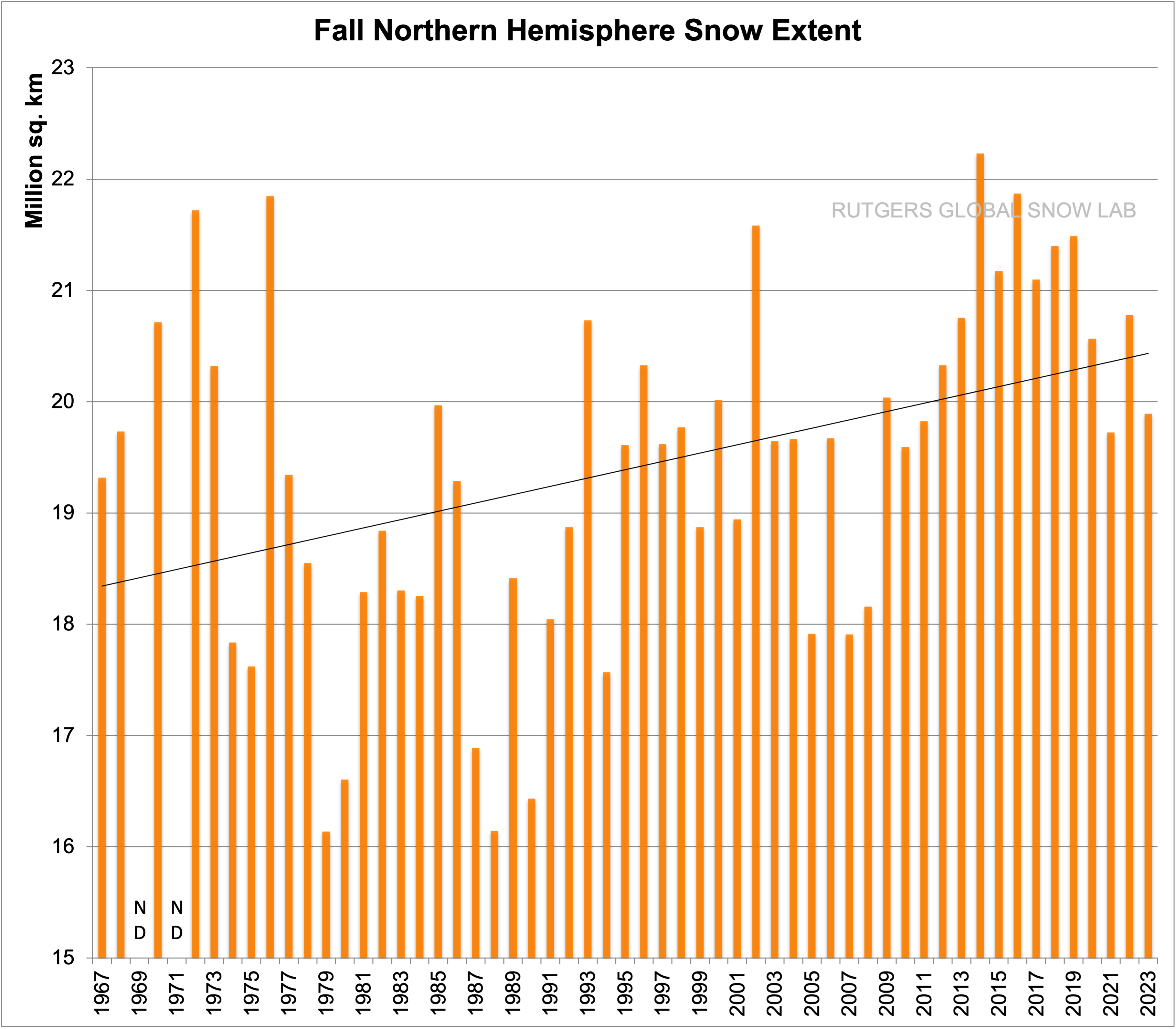
Early season snowfall across the NH has a strong upward trend:
Anyone who takes an unbiased view of the observations and knows a little about Earth’s relationship with the Sun will see the obvious.
Not sure I agree with the solar circular orbit around the barycenter, but I agree the solar and orbital influence on Earth’s climate is complicated.
My point in raising the circular orbit of the Sun is that I believe there is a HUGE amount of science to go on climate before anyone can claim it is settled.
Clearly the big change coming for the entire planet is glaciation of the NH. The ice mountains will make all land north of 40N uninhabitable. The falling oceans will make all ice free land cooler and probably less productive. Nearly all existing ports will need to be relocated.
Rather than pushing the CO2 scam, scientist should be focused on what drives glaciation. It its already apparent to me that Earth is into the next cycle with Greenlands leading the way.
Regarding the barycenter of the solar system and climate, the late Theodore Landscheidt wrote about it extensively, and even made some predictions decades ago. You will find some interesting reading by googling: landscheidt site:john-daly.com
Harold The Organic Chemist Says:
ATTN: Andy and Everyone
RE: CO2 Does Not Cause Warming Of Air.
RE: Comment #1
Shown in the chart (See below) is a plot of the average annual temperatures at Adelaide which shows a cooling from 1857 to 1999. In 1857 the concentration of CO2 in air was ca.280 ppmv (0.55 g CO2/cu. m.), and by 1999, it had increased to ca. 370 ppmv
(0.73 g CO2/cu. m.), but there was no corresponding increase in the city air temperature. A reason is that there was no warming of the air is because the amount of IR light absorb by this trace amount of CO2 is insufficient to heat up the air which has mass of ca. 1.2 kg /cu. m. at 20° C. Thus we can rule out that CO2 can have no influence on climate cycles. Note: No 60 year climate cycle signal in the 147 year temperature record.
The chart was taken from the late John Daly’s website: “Still Waiting For Greenhouse” available at: http://www.john-daly.com. From the home page, page down to:
“Station Temperature Data”. On the “World Map”, click on “Australia”. On the list of weather stations, click on “Adelaide”. This will bring up the chart for “Adelaide”. Use the back arrow to return to the list of weather stations. John Daly found over 200 weather stations that showed no warming up to 2002. You should read the essays listed at the end of the site.
PS: If you click on the chart, it will expand and become clear. Click on the “X” in the circle to return to comment text.
I enjoyed reading this summary, as well as your earlier summaries. It is hopeful to find a feature in the periodigram near one year, if anywhere. The other labelled peaks are far more uncertain in the periodigram, as you know. Periodigrams are subject to aliasing due to the length of the data set and/or Nyqvist sampling, etc. For example, Liseicki and Raymo (2005) stacked 87 benthic drilling sites (and later the number has increased to 180). The attached periodigram shows the orbital periodicities, plus a pesky, but obvious feature at 29Ky. That is not an expected period and it is not always as prominent. Worse, the most prominent feature near 100K years is a known period, but not the one which should produce the largest peak, nor much of a peak at all. The 100K period has produced many papers, but no clean answer as to its origin. Later analyses proceeded to seek power at the periods of Heinrich and D-O events. There are bumps near the right places, far smaller than those in the attached graph. Are they real and related to Heinrich and D-O? As a working hypothesis, one can assume so and seek proof. There are Ice Rafted Debris (IRD) data which plotted with 10BE and 14C show a significant correlation with solar activity and maybe Heinrich and D-O, but NOT CO2. That is leading, but does not make headlines. It is also true that the Jupiter-sun system has its barycenter outside the solar surface, which for the other planets are buried inside the Sun. The effects on the Sun are not known, as far as I am aware, although more hypotheses exist.
In short, there is a signal-to-noise problem. Some day, this will be sorted out, but not yet. It is useful to have such compilations as presented here to illustrate the data and the difficulties.
There is still a lot to learn, so much for “settled science.”
An important aspect of the Earth-Sun relationship is precession of Earth’s axis. This dominates the variation in solar intensity across the hemispheres. This year the summer solstice at 25N will average 469W/m^2 and 502W/m^2 at 25S – huge difference.
So the solar forcing observed on Earth is dominated by orbital precession. Axial obliquity and orbit eccentricity modulate the basic forcing caused by precession. I show how it is modulated on the attached chart that links sea level and July solar intensity at 15N:
 ?ssl=1
When you do the Fourier frequency components of sea level and temperature, the precession period dominates the changes in sea level and temperature. It is apparent visually as well. The 100 year cycle is a multiple of the precession rather than being related to eccentricity. With signal modulating, you get side bands and 32 years is a side band of 23kyr precession being modulated by by 39kyr obliquity.
A key understanding is that the land has a limited ability to carry ice. In the present era, the carrying capacity is limited to four precession cycles in most of the NH – Greenland the exception most cyclers of glaciation. When sea level is around 100m below the present level, the rate of glacier calving overwhelms the ocean ability to warm and snowfall cannot compensate for ice lost. Once the oceans begin to rise it accelerates as ice shelves uplift create massive icebergs that roam the northern oceans; to further cool the surface and reduce snowfall.
Once the CO2 scam is in the rear view, real science will improve our understanding of all these aspects that drive the climate..
Nice graph, thanks.
Then there is Svensmark’s theory of cosmic rays which when allowed through by a weak sun (low solar wind) tend to form low clouds, blocking the sun’s rays. The cosmic ray intensities also fluctuate. Thus, if cosmic ray intensity increases during a time of weak sun, you get cooling, as with the LIA. This apparently happens roughly every 1500 years, or has for at least the past 12,000 years. Low level clouds, or the lack thereof, driven by both cosmic ray fluctuations as well as solar wind fluctuations are probably the biggest climate driver of all. A further driver of cosmic rays would appear to be the Milky Way arms, as our solar system passes through them, intensifying those rays, thus cooling the earth. Although CO2 likely has some effect, it is puny in comparison.
Harold The Organic Says:
ATTN: Andy
RE: Articles On Climate Cycles.
RE: Comment #2
Here are the titles of a research paper and a monograph which I downloaded from the net over 15 years ago.
Research Paper:
“An oscillation in the global climate system of period 65-70 years” by
Michael E. Schlesinger and Navin Ramankutty, Nature Vol. 367, 24 February 1994,
pp 723-726″.
Using singular system analysis, they analyzed temperature data from 11 regions of the earth and found the 65-70 year climate cycle. There are 30 papers in the reference list.
Monograph:
“Cyclic Climate Changes and Fish Productivity” by
L. B. Klyashtorin and A. A. Lyubushin. Moscow Vniro Publishing 2007 223 pages.
There are over 240 references.
Using a stocastic model, they analyzed fish catches in the world’s fisheries for the last 1,500 years and temperature data and found there was a world 60-70 year climate cycle.
URL: http://alexylyubin.narod.ru/climate_changes_and-fish-productivity.pdf?
It quite was a chore typing all of this in the comment using one finger.
Thanks for the Schlesinger paper, I did not have that one. I did have Klyashtorin’s paper and read it. I referenced it in Climate Oscillations #4. The 60-70-year oscillation seems to be the most powerful from a global perspective.
The attached figure is from Schlesinger. It compares the global mean temperature anomaly (dashed line) to the regional simulated GHG-climate model result subtracted from the Hadley center gridded temperature anomaly for 11 regions. The regional variance explained by the solid regional line is EV, the correlation coefficient between the regional line and the global line is ρ, the period for the regional line is τ. All lines are detrended.
Pretty much what I found, the global mean surface temperature correlates to the North Atlantic region and nowhere else. It doesn’t even correlate well in the North Pacific.
‘The causes of climate change are a complex mixture of many natural cycles’
To add to the complexity, one must consider that the oceans act as an intermediary between the sun and the atmosphere.
The vast majority of solar energy, that reaches the earth’s surface, is absorbed in the oceans. And water evaporation from the tropical oceans is the mechanism by which the vast majority of this energy is then transferred to the atmosphere.
Thus, the delay between the time that solar energy reaches the earth’s surface and the time that it shows up in the atmosphere varies from the order of months, for solar energy that is absorbed near the ocean surface in the tropics, to decades, for solar energy that is absorbed by the oceans outside of the tropics.
From post:”‘The causes of climate change are a complex mixture of many natural cycles’”.
Dixie Lee Ray said the same thing when she was head of the Atomic Energy Commision back in Reagan era.
Dixy Lee Ray was very smart.
She often noted the following quote from some of the Greenpeace founders:
“It does not matter what is true, it only matters what people believe is true.”
From Environmental Overkill, by Dixy Lee Ray and Lou Guzzo
https://andymaypetrophysicist.com/2022/11/07/greenpeace-crimes-and-lies-updated/
Well, the IPCC has to exclude big or large natural fluctuations otherwise the idea of CO2 forcing cannot fly. So, all the cycles are nicely streamlined to show small variations and all the concentration is on CO2 because IF those cycles/ variables were greater you obviously cannot show the linear CO2 trajectory which is where the supposed danger lies.
Much of climate science has to do with trying to separate noise from signal and correlation/ causation of elements. It remains an intrinsic problem. We do not need to ‘solve’ it , although one tries, but we DO need to make people understand not only the complexity but the uncertainty of assumptions and especially assertions.
Exactly!
The climate system is naturally chaotic, as you imply, exhibiting large natural fluctuations. However the climate system is also able to ‘constrain’ this instability, maintaining ‘meta-stability’ in spite of these large natural fluctuations.
The whole CO2 story depends on an underlying assumption of inherent stability, that only a small fluctuation of a minor factor, such as the concentration of CO2, can disrupt. This inherent assumption is fundamentally at odds with both scientific knowledge and the earth’s history.
Andy, Bravo, Bravo! Your series has been enlightening. Having spent a lifetime measuring noise and vibrations in automobiles, I used to think that my analyses were difficult, but are trivial compared with yours. A few rotating tires and gears are nothing compared with climate cycles.
Living in Texas Hill Country, my climate is totally different than that of my two closest neighbors. I live on a west facing slope with strong afternoon sun. Across the street, the neighbors live on flat forested land stretching north. To the east, the neighbors get abundant cool morning sun. Multiply that by a few billion families on earth, and you get an estimate of the complexity of climate cycles. There is, no doubt, some grand equation that connects us all, but the terms would be a good approximation of infinity.
The AMO is always warmer during each centennial solar minimum, that’s not internal variability, it’s a negative feedback to changes in indirect solar forcing, and with a considerable overshoot.
Correlations of global sea surface temperatures with the solar wind speed:
https://www.sciencedirect.com/science/article/pii/S1364682616300360
Every other warm phase of the AMO is during each centennial solar minimum, so predictably the long term average AMO frequency is close to 55 years.
Centennial minima intervals vary between 7 and 12 solar cycles, so the AMO cycle lengths must vary according the centennial minima intervals. The Gleissberg cycle varies between around 80 and 130 years, it is not a fixed length, it’s just another name for centennial solar minima.
Centennial minima are a product of the first grand synodic period of Earth-Venus versus Jupiter-Uranus, Saturn is not involved. The planetary ordering of solar cycles is at heliocentric geometric syzygies and quadratures of those four planets, and as the orbits are elliptical, the timing of the centennial minima has to vary.
There is no 60 year cycle, and the idea that every third inferior conjunction of Jupiter and Saturn would create a 60 year envelope is bizarre.