By Christopher Monckton of Brenchley
As the third successive year of la Niña settles into its stride, the New Pause has lengthened by another month (and very nearly by two months). There has been no trend in the UAH global mean lower-troposphere temperature anomalies since September 2014: 8 years 5 months and counting.

As always, the New Pause is not a prediction: it is a measurement. It represents the farthest back one can go using the world’s most reliable global mean temperature dataset without finding a warming trend.
The sheer frequency and length of these Pauses provide a graphic demonstration, readily understandable to all, that It’s Not Worse Than We Thought – that global warming is slow, small, harmless and, on the evidence to date at any rate, strongly net-beneficial.
Again as always, here is the full UAH monthly-anomalies dataset since it began in December 1978. The uptrend remains steady at 0.134 K decade–1.

The gentle warming of recent decades, during which nearly all of our influence on global temperature has arisen, is a very long way below what was originally predicted – and still is predicted.
In IPCC (1990), on the business-as-usual Scenario A emissions scenario that is far closer to outturn than B, C or D, predicted warming to 2100 was 0.3 [0.2, 0.5] K decade–1, implying 3 [2, 5] K ECS, just as IPCC (2021) predicts. Yet in the 33 years since 1990 the real-world warming rate has been only 0.137 K decade–1, showing practically no acceleration compared with the 0.134 K decade–1 over the whole 44-year period since 1978.
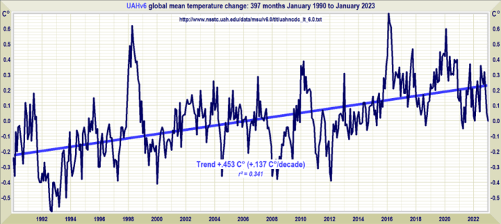
IPCC’s midrange decadal-warming prediction was thus excessive by 0.16 [0.06, 0.36] K decade–1, or 120% [50%, 260%].
Why, then, the mounting hysteria – in Western nations only – about the imagined and (so far, at any rate) imaginary threat of global warming rapid enough to be catastrophic?
How long is the cooling trend, 6-7 thousand years?
Make that 50 million years. Ahh, the Early Eocene days were warm days.
You don’t get weather like that any more. The planet is going to the dogs.
Indeed, our grandchildren will not know what the ‘climate change’ was.
Vuk,
For Australia, the Monckton method shows a negative temperature trend of 10 years 9 months, starting in March 2012.
If I wanted to spin a story, I could assert that no Aussie school child under 11 years old has felt any warming effect while being taught that global warming is an existential crisis.
Wake up, educators.
Geoff S
http://www.geoffstuff.com/uahfeb2023.jpg
The US 48 state average temperature trend using NOAAs USCRN weather station system has been relatively flat since 2005.
Global Temperature: | Watts Up With That?
USCRN affects 330 million people. While the global average temperature affects no one, because no one actually lives in the global average temperature!
We could say no US 48 state resident has experienced more than a tiny amount of global warming since 2005 — and that’s 18 years. That beats your 10 years and 9 months, using an official government temperature organization’s own numbers too!
RG said: “The US 48 state average temperature trend using NOAAs USCRN weather station system has been relatively flat since 2005.”
The trend is +0.58 F/decade (+0.32 C/decade). I invite you download the data and see for yourself.
RG said: “That beats your 10 years and 9 months, using an official government temperature organization’s own numbers too!”
Using the Monckton Method the USCRN pause is 0 months. That is a lot less than 10 years and 9 months.
I wrote that the US average temperature trend was relatively flat. I did not write that it was flat.
The trend appears to be flat since 2011. Thats from an eyeball view of the chart at the link below. I revise my claim to 11 years, rather than 18 years, and that still beats the Australians.
Those 11 years of flat temperatures included the largest 11-year increase of global CO2 emissions in the history of of the planet. And you can store your statistics where the sun don’t shine, bedofwax.
Global Temperature: | Watts Up With That?
Ignoring NOAA, here in Michigan there has been slight warming in the winters since the 1970s. I noticed mainly because we lived in the same home since1987 and four miles south in an apartment for 10 years before that. If we had moved 20 miles north in those years, the I might not have noticed.
I don’t need any government scientists to tell me how much warming I have personally experienced where I live.
Especially people from NOAA; who I do not trust. They have two different weather station systems with very different weather station siting. But somehow, magically, they both produce almost the same adjusted data. That is not by chance — hat is by science fraud, in my opinion.
What is the range of C/decade that would make something relatively flat?
relatively flat? maybe you head is relatively pointed
Here comes Masher the fool with brilliant not funny in any way put-down
USCRN affects 330 million people. While the global average temperature affects no one, because no one actually lives in the global average temperature!
you win stupidest argument ever.
You would be an expert on stupid, Masher.
The average temperature is not a real temperature, it is a statistic. A statistic is not an actual temperature.
I tried to explain this simply so even a 12year-old child could understand, Go out and find a 12 year-old child to explain it to you.
RG said: “The average temperature is not a real temperature, it is a statistic.”
The Tmax and Tmin you see reported for each station…both 1-minute averages. Do you think they aren’t real?
Because Tavg IS a statistic. What is the variance of that distribution. It is supposed to represent the midpoint of Tmin and Tmax.
Daytime temps resemble a sine curve, yet nighttime temps are an exponential decay. Sometime in late afternoon, the sun’s insolation energy is less than the earth’s radiation and the decay begins. Do you think Tavg is a true average temp or is it simply a statistic describing the midpoint between max and min.
Tmin and Tmax are averages too. And you’ve already said an average of an intensive property isn’t real. I already know your position on the matter because you’ve made it abundantly clear. I’m asking how deep Richard Greene’s conviction goes.
Again, you have no idea why the measurements are averaged. You are not a physical scientist and nothing in statistics will tell you why a 1 minute average is used.
Do you want to know why? My guess is that you really don’t care!
So you think the average temperature is Tmax and Tmin?
ROFL!!
Why do you think the “average” over 1 minute is used? My guess is that you have not one single clue as to why!
https://www.climate.gov/news-features/understanding-climate/climate-change-global-temperature
Earth’s temperature has risen by an average of 0.14° Fahrenheit (0.08° Celsius) per decade since 1880, or about 2° F in total.
The rate of warming since 1981 is more than twice as fast: 0.32° F (0.18° C) per decade.
2022 was the sixth-warmest year on record based on NOAA’s temperature data.
The 2022 surface temperature was 1.55 °F (0.86 °Celsius) warmer than the 20th-century average of 57.0 °F (13.9 °C) and 1.90 ˚F (1.06 ˚C) warmer than the pre-industrial period (1880-1900).
The 10 warmest years in the historical record have all occurred since 2010
UAH temperatures dropped below the zero line in January. If you ignore “trends”, and just trace your finger from the far right to the far left of the UAH graph, you discover our mean temperatures world-wide were the same as they were in May of 1980. Yes, that was the top of a peak and current temperatures are down at the bottom of the dip, but still, they are the same. In essence, we are back where we were, and we have spent trillions making much ado about nothing.
If the argument is that selecting a top of a local peak as the start is valid then surely the reverse is valid too. That gives us (-0.04 C – -0.67 C) / 461 months * 120 months/decade = +0.15 C/decade.
Bring back the dinosaurs!
Those were the days.
We get deer in our yard almost every day
Up to 14 at one time. After 36 years of watching them eat everything green, we could use some new entertainment. Dinosaurs would be exciting.
I have 40-50 at a time at my bird feeders. It is not cheap feeding them. Just before the cold comes and then afterwards when the ground is snow covered, they really hit it hard!
I have an 8 lb, squirrel proof feeder and two seed block cages I keep stocked. When the weather gets hard they will empty that feeder in two days and the seed blocks will be gone in 1 day.
I also cast feed on the ground for the ground feeders like the morning doves and the cow birds.
LIke I said, it ain’t cheap, and costs me about $30.00 a week to do it, but it is worth every dime.
Good job
We have a four-cake suet feeder and one thistle feeder. We also have a heated bird bath about 10 feet from our living room window. Entertainment for our indoor cat too.
We once had five deer lined up to drink some water from the bird bath. Two males got in a fight to see who would drink first. The males always go before the females.
I once helped break up a summer fight between two male deer whose antlers were locked together. They were tearing up the yard. Afterwards, I realized that was risky and I should have stayed away.
I forgot to mention two hummingbird feeders in warmer weather that the wife fills with freshly made sugar water every few days.
We’ve also had ground hogs, skunks, raccoons, opossum, rabbits, squirrels and hawks live in a nest next door — we used to have a lot of chipmunks but they apparently make good hawk food.
I love the animals but always chase pesky kids off my lawn. I think old guys are supposed to do that. It’s in the Constitution. … I could live without the skunks too. … Killed the moles with poison.
I had a kangaroo in my driveway once, and another on a walk near home late January. I live in an urban area.
No kangaroos here in Michigan. But have had one coyote, two foxes and many Jehovah’s Witnesses visiting in past decades.
We have white tails come through every once in a while. We’re a stopping place for a Raccoon family as they make their nightly rounds. Red fox, skunks, etc come through every once in a while.
The critters not welcome are coyotes and moles. Coyotes because they will go after the dog when we let her out on her lead. And moles, well the reason is obvious.
Had a Pileated Woodpeck stop buy in January. And then a red tail hawk came by trying to use our bird feeders as a hawk feeder. He was a young one and soon moved off to look for a better hunting ground.
Since I am coming and going at all hours for my job, I have to watch for deer on the road coming to my house. the road crosses two creeks and it is along that bottom land that the deer like to travel.
Dinosaur watching is a popular activity, with life lists.
My two seed block cages hang from a double shepherds hook outside a dining room window. As Sherry and I have our coffee we can watch them.
I believe the recent 2.8 million years have been the coldest of the last 200 million years including today. Maybe that’s the reason we call it an Ice Age. We are so lucky to live in an interglacial moment when places like Canada or Greta’s homeland are not under a mile of ice.
https://www.climate.gov/news-features/understanding-climate/climate-change-global-temperature
Earth’s temperature has risen by an average of 0.14° Fahrenheit (0.08° Celsius) per decade since 1880, or about 2° F in total.
The rate of warming since 1981 is more than twice as fast: 0.32° F (0.18° C) per decade.
2022 was the sixth-warmest year on record based on NOAA’s temperature data.
The 2022 surface temperature was 1.55 °F (0.86 °Celsius) warmer than the 20th-century average of 57.0 °F (13.9 °C) and 1.90 ˚F (1.06 ˚C) warmer than the pre-industrial period (1880-1900).
The 10 warmest years in the historical record have all occurred since 2010
It’s a modern millenarian apocalyptic secular movement. They flourish particularly around the turn of every millennium.
The human mind is too complex and has quirks that evolution hasn’t been able to iron out.
Ja. It is also what I said….
https://breadonthewater.co.za/2021/03/04/the-1000-year-eddy-cycle/
The primitive human brain is hard wired to respond to fear with heightened attention. It then looks for correlations to confirm there is a threat creating a false impression through narrow focus. Those who desire control over others know this can be used to increase their power.
The evolutionary escape is to understand the limitations and projections of the conditioned mind and examine how cause and effect brings everything into being.
It is easy to see through the fear mongering when you understand its purpose is to manipulate and control you.
I’ve noticed this for several decades now. Man always needs something to worry about. When I grew up, it was the cold war and nuclear annihilation. For a short period, it was terrorism. Big brother has tried to make global warming front of mind.
Now that the world is starting to cool again (my study of the matter is that the temperature varies from warmer to colder in multidecade cycles, moderated by our huge heat sink also known as the oceans).
Look back in history and you will always find something that man was told to fear.
As for global warming, I like to point to the earth’s warming at the end of the Younger Dryas period (~10C temp rise in a decade) when people spew the BS that the world’s temperature has never risen this fast before. The followup question is – do you think that rise was due to early man discovering how to burn coal for warmth?
I would not argue a “never before”, never is just too big a statement. However: How sure are you that you know how warm the Younger Dryas period was?
How do we know how warm the Younger Dryas period was? Warm??? Mate, it was perishing cold. Young Mr Dryas wrote it all down, and it’s now carefully reported in Wikipedia. They cite all the original Mr D manuscripts.
Or maybe it was Young Ms Dryas? That bit got lost.
How sure are you that you know how warm the Younger Dryas period was?
even when its cold the question “how warm was it ? means
what was the temperature.
Oops that was meant to be a reply to Steven Mosher’s reply to me.
The fastest warming ever is a primary lie the media sows to scare the uninformed. I don’t think that was zzz’s claim.
There are more than a few scientific papers on this subject. I’ve read papers dated from the late 90s to present time acknowledging this rapid heating.
As you know, NOAA is pushing the CAGW agenda, yet here’s a link from them on the Younger Dryas period. https://www.ncei.noaa.gov/sites/default/files/2021-11/3%20The%20Younger%20Dryas%20-FINAL%20NOV%20%281%29.pdf
Note this in paragraph one: The end of the Younger Dryas, about 11,500 years ago, was particularly abrupt. In Greenland, temperatures rose 10°C (18°F) in a decade (Alley 2000).
If you dig through other papers on the subject, you’ll find that this temperature increase has been noted worldwide in that time period.
So unless one says that this rapid temperature increase was due to man, my point here is that the climate can change significantly in short timespans due to natural causes.
“ the climate can change significantly in short timespans due to natural causes.” Common Sense. Not Taught. Not ‘Learned’.
Everytime I see the word “unprecedented” in the press, as they lament so called warming caused events, I ask myself a similar question.
“the BS that the world’s temperature has never risen this fast before.”
That claim came from taking the average increase in temperature over thousands of years from proxies and comparing it to the modern high resolution instrumental record. This is scientific fraud. The two data sets are like comparing apples to frogs.
Exactly right. This ”fast rate of temperature rise” would have happened countless millions of times. Scientists are to blame for not speaking out.
Hmmm. I see your point. Or, I’d see your point IF the modern instrumental record was unaltered. But it’s been altered so many times that it is no longer very accurate. Dr James Hansen not only altered the entire historical temperature database but he also did not save the unaltered data. And then there was the Australia BOM who altered their historical data with Acorn 2.0. https://wattsupwiththat.com/2019/02/22/changes-to-darwins-climate-history-are-not-logical/
I don’t have much faith in the modern historical temperature record, as it’s been heavily altered by people with a bias toward global warming.
My best bet for accuracy would be satellite. There can still be questions of bias in the tabulation. With millions (I assume) data points the tiniest rounding errors could add up significantly, and even with that resolution the data only covers a small fraction of the planet. If we are can panic over 1 or 2 degrees, the planet has much bigger threats to offer, that can make the pain even more exquisite.
Turkey.
Creating general fear is a premier political power play. Political power is always in demand by someone, so creating fear to further that power is always in play somewhere.
“When I grew up, it was the cold war and nuclear annihilation”.
Me too, in the 1960s. But I stopped worrying when we were told by our teachers that we would be safe hiding under our desks during a nuclear attack.
I got in a verbal fight with a grade school teacher when were asked to participate in an under the desk nuclear attack exercise. I had new dark color pants on and didn’t want to be laying on a dirty floor. The start of my career as a juvenile delinquent.
I doubt if hiding under a desk will save children from climate change.
Nice to remember that teachers were always so intelligent, even before the era of leftist brainwashing in schools.
LOL, yes. Same here on the nuke drills, except I wasn’t smart enough to say that hiding under a desk wasn’t going to save anyone from a nuke blast.
But I lived in an area that would have been a primary target – the Washington DC suburbs inside the beltway.
It didn’t matter where you lived. Someone would invent a reason that something near you would be a target.
Nah… the ‘nukers’ would aim for something of use.
At primary school, I had more fear & dread about Sister Mary Constanza and her cane than I did about a nuclear conflagration.
What if they wore a mask as well?
today people fear a green bogeyman that will force them to drive EVs and they fear not having copper,
just read the posts here for loads of fear mongering
Got yer battery car yet, mosh?
no car.
mosh: i think man will go to the moon
wuwt: oh ya, wheres your rocket.
i come here to see how stupid arguments can get, and im never disappointed by you guys
Hypocrite.
Steven Mosher said: “i come here to see how stupid arguments can get, and im never disappointed by you guys”
Here are some of my favorite arguments people have tried to convince me of.
~ The law of conservation of energy holds only after a period of time has elapsed.
~ The law of conservation of mass does not apply to the carbon budget.
~ It is not valid to perform arithmetic operation on intensive properties like temperature.
~ Ocean water below the surface does not emit radiation.
~ The Stefan-Boltzmann Law only applies if a body is in equilibrium with its surroundings.
~ Quantum Mechanics is completely deterministic.
~ If you utilize statistical inference then you aren’t doing science.
~ If you make predictions then you aren’t doing science.
~ Kirchoff’s Law prohibits polyatomic gas species from impeding the transmission of energy.
~ A sum (Σ[x]) is the same thing as an average (Σ[x]/n)
~ A quotient (/) is the same thing as a sum (+).
~ Computer algebra systems like MATLAB and Mathematica output the wrong answers when given the equations from the GUM.
~ The NIST uncertainty machine does not compute uncertainty correctly.
~ Category 4 Hurricane Ian was not even a hurricane because this one really small wind observation hundreds of kilometers from the radius of maximum was less than hurricane force.
And the list goes on and on…
But I don’t come here to see absurd arguments. I come here to learn first and because I still (perhaps naively) think that I can convince people of scientific truths using the consilience of evidence.
My point was not that we should fear not having copper. Sorry if I was unclear.
It was that copper will become much more expensive in the future as the ores being mined become progressively less rich in copper. And as a result, it is foolish to design an energy system dependent on copper.
Regards,
w.
Copper has been expensive enough that thieves will risk getting fried to steal it. Been going on for a long time now.
People under the influence of powerful drugs aren’t exactly thinking clearly. They steal the copper wire, or try to, because they are addicted to Chinese Fentanyl. Stealing energized wire could be done, but it requires specialized training, expensive equipment and huge <<redacted>>.
My point was not that we should fear not having coal. Sorry if I was unclear.
It was that coal will become much more expensive in the future as the ores being mined become progressively less rich And as a result, it is foolish to design an energy system dependent on coal.
Regards,
Mosh, first, we have ~130 years of proven coal reserves and about 20 years of proven copper reserves. Please tell us which one will increase in price faster?
Second, we are being forced by governmental edicts and subsidies to shift to a copper based energy system. If it were a good idea the shift would occur by itself.
But I suspect you know all of that, and are just trying to stir the pot …
My best regards to you, get well, stay well,
w.
Coal is just something to burn to heat water to make steam to use as a working fluid for the steam turbines which drive the generators,
There are alternative heat sources.
An engineer friend from Uni used to consult on converting coal fired boilers to gas when coal was relatively expensive, and converting gas to coal when gas was relatively expensive.
NO! What we fear is overbearing government working for their own and other agendas that have a negative effect on the liberty and welfare of their citizens, and the bone heads that support those totalitarians.
The Green Bogeyman is real. That’s how we got in this screwed-up position in the first place.
NetZero, the Green/Authoritarian Delusion.
real? what screwed up position
Look around you.
Good Grief!
Yes, politics, especially left wing, as usual. H.L. Mencken said:
The whole aim of practical politics is to keep the populace alarmed — and hence clamorous to be led to safety — by menacing it with an endless series of hobgoblins, all of them imaginary.
Ah, last century we had ‘flappers’ …This century they are flapping like a big girls blouse…
Leftism (anyone who wants more government power) uses fear to create a demand for more “government powers”, This has been a strategy for many centuries. Not just once in a while — at all times.
And this is not secular. Religions use tall tales to create fear (in the opinion of this long-term atheist) of God and hell to control people. Also, the claim of heaven. It’s all nonsense to me, just like the fear of the future climate.
I see little difference between people who fear God and hell, versus other people who fear climate change. Unproven fears are irrational. At least the religions have some good commandments. The Climate Howlers don’t even have that. They could not care less about actual air, water and land pollution in Asia, for one example. Instead, they falsely define the staff of life, CO2, as pollution. The climate change secular religion is of no value to mankind.
Honest Climate Science and Energy
In addition, The Golden Rule is one ‘commandment’, and is one which covers any and all. It appears to be as difficult to apply that ONE to one’s life, as to apply any few of the various.
Yes!
Thank you
As of this month we have cooled 0.7C the last 7 years. Hard to keep the existential crisis narrative going with this data but that won’t stop the media from pushing the irrational fear mongering incessantly.
The trend is at 0.24 C / decade since 2016. If this continued the cooling would get hard to ignore.
The trend here is +6 deg C PER DAY this weekend. Now that’s really hard to ignore.
That trend is because of a rare triple La Nina. The next El Nino will change the slope dramatically.
From what I’ve heard based off the amount of warm water volume, the upcoming El Niño will present a 2009/2010 like situation.
We will see. I expect the trend to increase over the next few months due to this La Nina. I’m hoping the next ENSO phase is neutral as that will give us a better feeling for where we are. Of course, the big change will occur when the AMO goes negative. Coming soon to a planet near you.
I don’t think that we will see cooling in the long run until the SSTS in the oceans drop. And that isn’t happening yet.
That would be a good thing.
At the last AMO transition there’s was a reduction in cloudiness. If the reverse happens in the coming AMO transition, this should cause ocean cooling.
Any cooling is counter to the claims of CO₂ addled.
They already choke when CO₂ levels continue to increase while temperatures dive.
That’s when they start claiming CO₂ causes every kind of weather; cold, hot, rainy, arid, stormy, windy, calm, jada jada jada.
Within a few years, they’re likely to flip the narrative back to global cooling. If you look through the decades with news articles, you’ll find this alternating narrative of ‘the world’s on fire’ to ‘an ice age is coming’ is a common theme that runs for a few decades and then flips to the other fear.
I had a link to a Canadian article about this, but lost it a few years ago. The article went back to the early 1900s where it was cooling, then warming, then cooling, now warming.
The cooling and warming predictions pre-1970s were usually from individual scientist crackpots. The 1970s cooling warnings were bigger, but still a small minority of all scientists. The current global warming warnings are a 59% majority, by a libertarian survey last year — 59% believe in imaginary CAGW. And at least 99.9% believe in real AGW of some amount, no matter how small. But climate change means scary CAGW, not harmless AGW.
Richard, that’s likely due to the lack of climatologists and grant money in prior to the 1980s. Now, the amount of money spent on the subject dwarves previous decades. And that grant money delivers the study results desired by government.
Does CO2 warm the earth? Maybe. My opinion is that it does warm the earth but its impact is de minimis. There are simply too many variables to isolate the impact of a single input into the world’s climate. I think that the earth is warmer today than when I grew up in the 60s, but I attribute that to natural temperature variation on a multidecade heating/cooling cycle for the earth.
We can definitively say that CO2 levels have risen annually since it was first regularly measured (1958), yet the world’s temperature has fluctuated in that time. The correlation is not as strong as it’s hyped to be.
”And at least 99.9% believe in real AGW ”
What is this ”believe” nonsense. They either know or they don’t know.
They know CO2 is a greenhouse gas
They know air pollution blocks sunlight
They know a warmer troposphere holds more water vapor
They know human adjustments to raw temperature data, and infilling, could account for a significant portion of the claimed global warming in the past 150 years.
What else do scientists need to know to believe in AGW?
RG said: “They know human adjustments to raw temperature data, and infilling, could account for a significant portion of the claimed global warming in the past 150 years.”
It’s the opposite. Adjustments reduce the amount of warming relative to the raw data over the last 150 years. Hausfather provides a brief summary of how the adjustments affect the long term trend.
bgwxyz reiterates his approval of fraudulent data mannipulations.
BedOfWax is a liar or a fool, or both/
The 1940 to 1975 period had added warming because the global cooling with CO2 rising reported in 1975 was inconvenient for the CO2 is evil narrative that fools like BedOfWax believe in. That was science fraud, and you know it.
In the US the mid-1930s were warmer than even 1998 with that huge El Nino heat release, but not anymore.
Zeke H. is a deceiver.
His “infamous” argument that climate models are accurate used TCS and RCP 4.5, which the IPCC never publicizes, rather than the popular ECS and RCP 8.5 which the IPCC does publicize, and very likely over predict global warming.
Zeke H. Sleight of hand that you warmunists.loved.
Anyone wo thinks there was a real; global average temperature before the 1940s, with so few Southern Hemisphere measurements, is a liar. Pre-1900 is mainly infilling, not data. Still a lot of infilling today — you have no idea how much because you don’t care.
The chart you presented is bogus — it completely ignores the huge data changes for the 1040 to 1975 period based on what was reported in 1975 versus was reported today.
Honest Climate Science and Energy: NOAA US average temperature from 1920 to 2020, Raw Data vs. Adjusted Data presented to the public (science fraud)
Honest Climate Science and Energy: Pre-1980 global average temperature “revisions” from 2000 to 2017 (science fraud)
Honest Climate Science and Energy: Click on READ MORE and watch US climate history get changed to better support the CO2 is evil narrative
Honest Climate Science and Energy: Global Average Temperature History Keeps Changing — National Geographic in 1976 versus NASA-GISS in 2022
Honest Climate Science and Energy: Watch climate history change to better support the false CO2 is evil — it’s magic science fraud
The graph includes all adjustments. This is probably the source of confusion. If you are used to getting your information from contrarian bloggers then you probably were only aware of the adjustment that bump up the temperature anomalies later in the period and had no idea about the more significant bump up earlier in the period. I also recommend reading about the details of the adjustments. They are important because there are subtle implications when deciding which of the seemingly equivalent approaches of bumping up before the changepoint or nudging them down after the changepoint to correct the changepoint bias.
BTW…all of the adjustments and infilling in the traditional surface datasets are done in UAH as well. In fact, UAH not only performs the same adjustments, but they do so more aggressively and then perform other adjustments that the surface datasets don’t even have to worry about. Most people are not aware of this.
More fraud, par for the course for CAGW kooks.
bgwxyz: “UAH does data mannipulations, so it must be ok!”
Do you expect to be taken seriously after making statements like this?
“contrarian bloggers” — ah, poor baby
“They are important because there are subtle implications when deciding which of the seemingly equivalent approaches of bumping up before the changepoint or nudging them down after the changepoint to correct the changepoint bias.“
No, it is all unscientific fraud, and you are a disgrace to the profession.
karlomonte said: “bgwxyz: “UAH does data mannipulations, so it must be ok!””
Can you post a link to the post in which those exact words you have in double quotes appear?
Its a paraphrase, you clown.
The global warming religion posits that warming since 1950 is primarily anthropogenic and that it is somehow remarkably different from all warming periods in the past. The sharp pre-anthropogenic warming of ~1910-1945, and the overall warming trend from 1880-1945 show this to be evidently untrue. So Hausfather cooks up a reason to warm the entire period of 1880-1940, thereby vastly reducing the warming that the new Climate Faith holds cannot have been possible prior to 1950.
The fact that this reduces the amount of warming relative to the raw data over the last 150 years is not the relevant issue. What is relevant is that Hausfather’s adjustment largely erases the inconvenient “pre-anthropogenic” portion of the overall warming, thereby making the climate religion look less ridiculous. This should be rather obvious.
“The cooling and warming predictions pre-1970s were usually from individual scientist crackpots. The 1970s cooling warnings were bigger, but still a small minority of all scientists.”
I wouldn’t say that. The climate scientists were reporting on actual cooling. It cooled significantly from the 1940’s to the late 1970’s by about 2.0C (according to the U.S.temperature chart). No crackpottery there.
Now claiming the world was going into a new Ice Age might be a little bit much, but the climate scientists of the era did have a reason to note the cooling that was taking place at the time.
I was there. I saw all these claims about human-caused global cooling. At first, I thought maybe the climate scientists claiming humans were causing the cooling might have something, so I waited for them to present some evidence proving their case. And I waited, and I waited, and I waited and I waited. And I’m still waiting to see some proof of their claims.
So, when the human-caused global warming crew showed up claiming humans were causing the Earth to warm, I was naturally skeptical from my earlier experiences with these unsubstantiated climate claims, and to this day have not seen one bit of evidence proving humans are causing the Earth’s climate to change. Either way, cold or hot.
I wish I had the internet back in the 1970’s. I would have blistered the ears of all those charlatan climate scientists.
WUWT is like Heaven to me. I get to say just what I think about modern day climate science. 🙂
The reason for that uptick in hysteria is precisely because the facts are beginning to give the lie to climate alarmism, hence it must be restated at each and every opportunity.
Disagree
Hysteria must escalate because it loses its ability to scare people if it remains the same decade after decade.
This is the “Worst than we thought” propaganda strategy.
The actual temperature is not changing enough for many people to notice where they live. People rarely know “the facts”. They usually “know” what they are told by government authorities (who can’t be trusted, but they usually are trusted).
So the climate propaganda must escalate to be effective in creating fear. And creating fear gives leftists in power the opportunity to expand leftist government powers. Which they do. Never letting a crisis go to waste — whether a real Covid crisis, or a fake climate crisis.
.
Isn’t it 102 months?
https://woodfortrees.org/plot/uah6/plot/uah6/last:102/trend
I make it 102 months is you count the start month August 2014 to the end of Jan 2023.
Slope is -2E-05x in Excel notation.
Geoff S
Thanks, Christopher, for continuing to research and present it.
Regards,
Bob
Mike, how very kind and polite you are. The real thanks should go to Roy Spencer and John Christy, who have kept the UAH dataset honest when all others have tampered with theirs.
Which Christy and Spencer do VOLUNTARILY without payment!
Therefore, no financial conflicts of interest are possible.
No Christopher. My thanks for the post go to you. As you will recall, I used to prepare graphs of climate-and-weather-related data and discuss them in blog posts that were cross posted here at WUWT, so I know how much work goes into what you prepared above and into responding to comments.
Regards,
Bob
PS: I’ve been called lots of things, but this is the first time I’ve been called Mike.
I predict much whining.
You mean our biggest threat is all this global whining?
I think you are onto something important here.
The Climate Howlers do Global Whining
I like that and will use it.
As a blog editor, if I read something good, I steal it.
And please note how I am now confirmed as a psychic prophet…
There are a couple of problems with this type of analysis. One is that it does not adjust the statistics for autocorrelation.
The Hurst exponent of the UAH MSU dataset is 0.82. This means that the “effective N”, the number of data points for statistical purposes, is only 9 …
Now, this doesn’t remove the statistical significance of the trend in the full dataset. Here’s that calculation.
With a p-value of 6.30e-5, the trend is obviously statistically significant.
However, properly adjusting the analysis for autocorrelation means that shorter sections of the dataset cannot be said to have a statistically significant trend. Here, for example, is the same analysis for the most recent half of the UAH dataset. There, the effective N drops to a mere three data points.
With a p-value of 0.128, we cannot say that there is a statistically significant trend in the latter half of the MSU data.
As a result, I fear that the analysis of Lord Monckton isn’t valid.
Finally, it should not be a surprise that there are periods of increase and decrease in temperature data. Here, for example, is a breakpoint analysis of fractional Gaussian noise (FGN) with a Hurst exponent of 0.8, with an underlying trend added to the FGN.
Note the similarity to a natural temperature dataset. However, this is just random fractional Gaussian noise plus a linear trend. We know for a fact that there is an underlying increasing trend throughout the data … but despite that, there’s a decreasing section from 1980 to 2000 … is this a significant “pause”?
w.
I was thinking the same thing. e.g. How likely is it to find periods with a valid trend in a volatile, heavily censored dataset? We need a satellite and a time machine to gather enough data to support anything.
nope. satellite data is heavily censored and adjusted. 100 or so locations
will get you a good dataset.
Shen, S. S. P., 2006: Statistical procedures for estimating and detecting climate changes, Advances in Atmospheric Sciences 23, 61-68
You aren’t going to get it. In fact, UAH is one of the most heavily adjusted datasets in existence. And their infilling technique interpolates missing values (and there are a lot) up to 4160 km away spatially and 2 days temporally. Compare that with GISTEMP which only interpolates using data from 1200 km away spatially with no temporal infilling.
Year / Version / Effect / Description / Citation
Adjustment 1: 1992 : A : unknown effect : simple bias correction : Spencer & Christy 1992
Adjustment 2: 1994 : B : -0.03 C/decade : linear diurnal drift : Christy et al. 1995
Adjustment 3: 1997 : C : +0.03 C/decade : removal of residual annual cycle related to hot target variations : Christy et al. 1998
Adjustment 4: 1998 : D : +0.10 C/decade : orbital decay : Christy et al. 2000
Adjustment 5: 1998 : D : -0.07 C/decade : removal of dependence on time variations of hot target temperature : Christy et al. 2000
Adjustment 6: 2003 : 5.0 : +0.008 C/decade : non-linear diurnal drift : Christy et al. 2003
Adjustment 7: 2004 : 5.1 : -0.004 C/decade : data criteria acceptance : Karl et al. 2006
Adjustment 8: 2005 : 5.2 : +0.035 C/decade : diurnal drift : Spencer et al. 2006
Adjustment 9: 2017 : 6.0 : -0.03 C/decade : new method : Spencer et al. 2017 [open]
That is 0.307 C/decade worth of adjustments jumping from version to version netting out to +0.039 C/decade. And that does not include the unknown magnitude of adjustments in the initial version.
“As a result, I fear that the analysis of Lord Monckton isn’t valid.”
I have that fear too. The analysis won’t stand up to any kind of uncertainty analysis, Hurst or otherwise.
I show trends with uncertainty calculated using a Quenouille correction for autocorrelation. This is equivalent to an Ar(1) model. For UAH V6 fron August 2014 to January 2023, I do indeed get a slightly negative trend, -0.027°C/Century. But the 95% confidence intervals are from -2.838 to 2.783°C/Century. That is, you can’t rule out an underlying trend of 2.783°C/Century, which is higher than predicted by the IPCC. That is because of the short interval on which the trend is calculated.
Is the 30 year interval climate “science” uses too SHORT?
Of course it is.
Any interval would, by necessity, be over 10,000 years since that is back to the beginning of this interglacial period. So we are looking at the “climate” and temperature trends of an interglacial, and MUST include that ENTRE period if we wish to determine if there are any changes in trends caused by CO2.
Without that entire period, we cannot eliminate natural variation as the cause of the warming of the recent years. Heck, climate “scientists” have NO explanation of the very warm 1930s, or how it got so cold in the LIA, or so warm in the Roman optimum or Medieval Warm Period.
All of climate “science” is a fraud if the “average” of the models can not be used to hind cast those periods back to the year 0. Heck again, the models can’t even hind cast to the year 1900, 50 years after the end of the LIA.
It is all a very scary and very expensive fraud that is costing the poorest or the world a much better life. Since WWII, there have been skirmishes and a cold war, but no MAJOR conflicts involving the majority of the world’s nations and ALL of society should have been rising on the rising tide of excess production of houses, household items, food production, clean water and improved sanitary waste systems and LOWER “energy” expenses along with greater “energy” availability.
60 years of very good, overall, worldwide conditions wasted for the poor of Asia and Africa, especially, but ALL worldwide poor generally especially over the last 30+ years.
Nick, please defend you position of promoting the climate hysteria agenda in relation to the effect on the poor.
Thank you in advance,
Drake
In theory adding CO2 to the atmosphere all else being equal would increase temperature.
Climate variations prior to around 1880 when the CO2 concentration started to increase are irrelevant to the current climate that is the product of the effect of CO2 forcing and ongoing natural fluctuations acting on various time scales at times enhancing the warming and at times countering it.
As you say the inevitable economic advancement of world’s poor is all that matters in the end.
An excellent comment, Drake.
We live in the best climate in 5,000 years, based on climate proxies, and should be celebrating our current climate. Living during a warming trend in an interglacial is about as good as the climate gets for humans and animals on our planet. The C2 plants would prefer two to three times ambient CO2, but 420ppm is a good start — the best CO2 level for C3 plants in millions of years.
That a trend is not significant doesn’t mean it is not real. I called the attention to the change in Arctic sea ice in 2015 and was told the same. Now the new trend is 15 years old, and the “experts” are scratching their heads.
“That a trend is not significant doesn’t mean it is not real”
Indeed so. But it is a question of what you can infer from it. Clearly here we are asked to infer that it isn’t really warming. But what the insignificance says is that it really could be warming at quite a high rate, with overlying random factors (weather) leading to a chance low result.
The chance for any one instance is low (2.5% at the CI limit). But it becomes much higher if you select from a range of possible periods on the basis of trend. And that is exactly what Lord M’s selection procedure does.
No, I don’t “select from a range of possible periods on the basis of trend”. I calculate the longest period, working back from the present, that exhibits a zero trend or less. By that definition, which is made explicit in the head posting, there is only one possible period.
Since I draw no conclusion from the zero trend except that it provides a general indication that there is not a lot of warming going on, it is fascinating how upset the climate fanatics are about these simple graphs.
If it were indeed true that “it could be warming at quite a high rate”, then it would also be true that it could be cooling at just as high a rate. With so absurdly large an error margin, one wipes out the global warming problem altogether. For Mr Stokes is, in effect, admitting that climate scientists have no idea how much it is warming or cooling, or even which effect is predominant. If so, there is no legitimate basis whatsoever for doing anything at all to cripple the economies of the hated West in the specious name of Saving the Planet.
Stokes is just a propagandist shill for the IPCC, has no compunctions against posting anything that he knows to be false, to keep the hockey stick alive.
“No, I don’t “select from a range of possible periods on the basis of trend”. I calculate the longest period, working back from the present, that exhibits a zero trend or less”
The second sentence describes exactly the process of ““select from a range of possible periods on the basis of trend””
“With so absurdly large an error margin, one wipes out the global warming problem altogether.”
The error margin is just a consequence of your decision, against much advice, to try to make inferences from short term trends. That difficulty is present in any kind of data, and says nothing about global warming.
Climate scientists look at much longer time periods where the trend is indisputably positive.
Nick,
How many days of daily data do you recommend to define a short term trend? For making inferences? Change happens forever over a range of many orders of magnitude of time. You are selecting “short term” to suit your argument in the sense of “You are wrong because you used too short a short term”. Does not compute. Geoff S
Geoff,
As I showed with diagram, you can calculate the error bars, and they diminish as the term gets longer. You can make inferences accordingly.
Mr Stokes is, as usual, on a losing wicket here. I do not “select from a range of possible periods on the basis of trend”. I take a single trend – zero – and then simply enquire how far back one can go in the most trustworthy of the global-temperature datasets and find a zero trend. It is a matter of measurement by the satellites and calculation by me, using the method which, whether Mr Stokes likes it or not, is the method most often used in climatology to derive the direction of travel of a stochastic temperature dataset. If he wishes to argue that climatology should not use the least-squares linear-regression trend, then his argument is with climatology and not with me.
Mr Stokes is at his most pompous when he is most clearly aware that he is in the wrong and is not going to get away with it. For a start, we are not going to take “advice” from a paid agent of a foreign power.
Secondly, if Mr Stokes would take some lessons in elementary statistics he would realize that a zero trend has a correlation coefficient of zero (all one has to do is look at the diagram in the head posting, which is worth a read). What that means is that at any moment the trend might diverge in one direction or another, since the fact that it is zero gives little indication of what may happen next.
Thirdly, it is self-evident that the longer the period of data the narrower the uncertainty interval.
Fourthly, the effect of the uncertainty interval is to lengthen, not to shorten, the period over which it is uncertain whether there has been any global warming or not. The 101 months shown in the head posting is thus a minimum value.
Finally, I do not draw any “inference” from the fact that there has been no global warming for almost eight and a half years. I merely report the fact, explain how I derived it, compare it with the full dataset precisely to avoid the nonsense allegation of cherry-picking, and point out that the longer the zero trend becomes, and the more frequent such long trendless periods are, the clearer it becomes, and the more visible it becomes, that the rate of global warming over the past 33 years since IPCC (1990) is well below half what was then confidently predicted.
To all but those with a sullen vested interest in the Party Line, such observations are of more than passing interest.
“For Mr Stokes is, in effect, admitting that climate scientists have no idea how much it is warming or cooling, or even which effect is predominant.”
You put this in a previous post in the thread. You nailed it!
“point out that the longer the zero trend becomes, and the more frequent such long trendless periods are, the clearer it becomes, and the more visible it becomes, that the rate of global warming over the past 33 years since IPCC (1990) is well below half what was then confidently predicted.
I like the way you state this. It’s not that CO2 doesn’t have any impact on temperature but that it is far less than predicted – which also means that other control knobs can mask CO2 contributions rather easily. Tying all temperature increase to CO2 is just plain wrong. It then becomes a matter of trying to identify the entire range of contributions and when+how they impact temperature.
It is obvious when the Party Line has been shown to be bankrupt when all they have is to blindly press the downvote buttons, as is the case with your carefully crafted and succinct comments here.
If that were actually your selection criteria you would have to stop when you got to January 2022 because your 0 or negative trend would flip positive:
https://woodfortrees.org/plot/uah6/from:2022/plot/uah6/from:2022/trend
So it seems that there’s more to your selection than starting at the present day and seeing how far back you can get a flat or negative trend.
But as Nick shows it is all silliness, since you never actually consider the confidence intervals of your trends.
My thoughts entirely.
We do not use these numbers to predict or hindcast.
The main reason why I am now making an Australian subset each month is to keep alive the possibility that a cusp is under way. Caution is urged in case it foreshadows a temperature downturn.
I have also started an informal comment along the lines that if I wanted to spin a weather story, I could claim that children under 11 here have not felt global warming, despite CO2 increases.
Geoff S
I just look at when our gently warming globe first achieved January’s UAH temperature.and that’s 1988. So no warming for over 30 years
I don’t think we are being asked to infer anything except the obvious, that the surface is not warming faster over time, as it should according to a popular hypothesis.
The existence of multi-year periods of cooling is obvious and expected, but they should become less frequent and shorter if the warming accelerates as expected given the CO2 acceleration. The observation is contrary to the expectation, and Lord Monckton reminds us every month about it. Considering that we are reminded every single day how awful climate change is and how guilty we are, I don’t find his lordship’s reminders out of order.
I am most grateful to Mr Vinos for his kind comment. It is indeed interesting that the rapid decadal rate of warming so confidently predicted in Charney (1978), IPCC (1990) and, most recently, in IPCC (2021) is not coming to pass.
JV said: “he existence of multi-year periods of cooling is obvious and expected, but they should become less frequent and shorter if the warming accelerates as expected given the CO2 acceleration.”
I’ve not heard that hypothesis before. When I get time I’ll look at the CMIP model data and see if the frequency of pauses increases or decreases with time. There is so many little pet projects like these on my plate already though…
I did test the hypothesis that the expectation is for a decrease in the frequency of pauses using the CMIP5 data from the KNMI Explorer. There was no change in the frequency of pauses from 1979 to 2100.
The percent of time we expect to be in a pause depends on the length of the pause. For a 5 yr pause it is 30%. For a 10yr pause it is 13%. And for a 101 month pause like what is occurring now it is 18%.
What does this tell us? Despite Monckton assertion to the contrary it is not unexpected or even notable that we find ourselves in a pause lasting 101 months.
I encourage everyone to download the data from the KNMI Explorer and see for yourself.
And now he tells how he thinks the CHIMPS garbage-in-garbage out “climate” models are somehow valid.
Your need to apply statistics to obtain a looong trend from what appears to me to be a control system with short term excursions is unexplainable. Have you ever done control charts to see if these excursions are out of control?
When Nick the Stroker agrees with Willie E., I know I am living in bizarro land. That is impossible. I’m going back to sleep and hope this agreement has disappeared by the time I wake up. A Willie E. versus Nick the Stroker argument is a highlight of this website.
That is, you can’t rule out an underlying trend of minus 2.838C per century either. But the hypothesis that the trend is not statistically different from zero cannot be rejected. Thus your analysis, using a better technique more appropriate to the data, supports Monckton’s conclusions. The width of the confidence intervals is being driven by the extreme heteroscedascity in the data around the El Nino spike.
What is perhaps rather more revealing is to evaluate how much trend there is across the whole dataset in an AR1 model. When you do that the confidence intervals narrow considerably, but the estimate for the trend drops to an unexciting third of a degree per century.
Don’t panic.
“but the estimate for the trend drops to an unexciting third of a degree per century”
Really? I get 1.33°C/Century, in agreement with Roy Spencer’s calculation. And it is a bit more exciting down here where we live.
UAHV6:
Temperature Anomaly trend
Jan 1979 to Jan 2023
Rate: 1.332°C/Century;
CI from 1.013 to 1.651;
t-statistic 8.180;
RSSV4: 2.112°C/Century;
GISS: 1.868°C/Century;
HADCRUT 5: 1.887°C/Century;
(all except UAH to Dec 2022)
Mr Stokes is perhaps unaware that RSS, which showed a sudden uptick in its warming rate just a month after one of the Pause graphs here was debated in the U.S. Senate by Senator Ted Cruz, uses a defective satellite dataset that is now out of date. Without it, RSS would show much the same warming as UAH.
As to HadCRUT5, Dr Spencer has recently written at his excellent blog about the substantial influence of the urban heat-island effect on this and other terrestrial datasets.
Hmm. Tony Heller predicted that the RSS would suddenly change to showing more warming a couple months before it actually did.
Collusion Is Independence | Real Science (wordpress.com)
And then recently showed that what they have done is move their reported temperatures up to the top limit of the error bars in order to be in closer agreement with NASA data.
Adjusting Good Data To Make It Match Bad Data | Real Climate Science
Nick,
For monthly UAH Australia, from the 2016 high to the 2022 low I get a trend of nearly MINUS 30 C per Century equivalent over 6.5 years, in a time of CO2 induced catastrophic global warming, but I only quote this number to show absurdity of data torture.
Geoff S
Did you use an AR1 model for that, or just OLS? If I use OLS I get results that agree with yours. But the data are clearly autocorrelated, so OLS in NOT appropriate. Try again.
AR1 vs OLS makes very little difference. I get 1.33 with OLS, 1.30 with AR1. Here is my R working:
There is very little need to hunt for autocorrelation in the global temperature record, though it is a relevant consideration in the regional records thanks to seasonality. If the uncertainty in the UAH datea is indeed +/- 0.28 K/decade, as Mr Stokes suggests, then there subsists no basis whatsoever for the sedulously-peddled conclusion that we must Do Something to Save The Planet, because we have no idea whether the globe is warming rapidly or cooling rapidly.
I prefer to base my analyses on the real-world data and the uncertainty intervals issued by the keepers of the datasets. Those intervals are considerably narrower than Mr Stokes’ interval. If, therefore, Mr Stokes thinks the uncertainty interval is greater by an order of magnitude than the keepers of the datasets say it, then he should take up the matter with official climatology and not with me.
Professor Jones at the University of East Anglia, who used to keep the HadCRUT record, was happy to recommend the simple least-squares linear-regression trend as the best way to get an idea of the direction of travel in global temperature datasets. I do not claim anything more than that the least-squares trend has been zero for 101 months. I do not base any prediction on this fact: I merely report it, as well as the 44-year trend on the entire UAH dataset, for context.
The truth is that the world is not warming anything like as fast as had been, and still is, predicted. No amount of fluff and bluster will conceal that fact.
And there is absolutely no reason to try cramming battery cars down the throats of the entire world population.
“There is very little need to hunt for autocorrelation in the global temperature record”
The residuals are autocorrelated, and you absolutely have to allow for that in the confidence intervals. To show what is going on here, I plot the trends for each interval ending at present (Jan 2023). The start of the interval is shown on the x axis. Near 2023, the intervals are short, and the trend is wildly variable. As you go back in time (longer periods) the trend settles to a generally positive value (1.3 at 1979). Between the short term gyrations and the stabler long term, it crosses the axis one last time at August 2014. That is the point Lord M calls the pause.
I have plotted the confidence intervals in color. Blue is the OLS 95% CI, calculated as if there were no autocorrelation. It diminishes as you go back in time, and the trend stabilises. But there is autocorrelation, so OLS exaggerates the confidence. I have plotted the Ar(1) CI’s in red. They are more than double the breadth. The most recent year in which you can be 95% confident that the trend is positive is about 2011.
Mr Stokes digs himself further and further into a hole of his own making. Consider the entire UAH dataset, and compare the observed 0.134 K/decade warming rate since December 1978 or the observed 0.137 K/decade warming rate since January 1990 with the predicted 0.3 K/decade warming rate in IPCC (1990, 2021).
One of two conclusions follows. First, that the real-world rate of warming is indeed well below half what was originally predicted and is still predicted, strongly suggesting at least one systemic error in the models, in which event the expenditure of trillions, bankrupting the West, will achieve nothing.
Secondly, that the uncertainties in measurement of global temperature are so large that we are incapable of drawing any conclusion at all about whether or at what rate the planet is warming or cooling, in which event there is no empirical method by which the rapid-warming hypothesis that Mr Stokes and his paymasters so cherish may be verified, in which event it is merely a speculation that has no place in science.
Furthermore, I performed a detailed autocorrelation analysis on the datasets a few years ago, and found that there is very little of it in the global datasets, though it becomes noticeable in the regional datasets.
Stochasticity and heteroskedasticity are of more significance than autocorrelation in the global datasets. And, as I have pointed out to Mr Stokes before, it is official climatology that likes to use the least-squares linear-regression trend as the simplest way to get an idea of the direction of travel of the global-temperature datasets. If he wishes to quarrel with that custom, let him take up the cudgels with official climatology and not with me.
And once again, all they can do is push the downvote button…
CMoB said: “First, that the real-world rate of warming is indeed well below half what was originally predicted”
You can say that as many times are you want (and undoubtedly will), but it won’t make it any less wrong than any of the other times you’ve said it over last decade. As we’ve repeatedly shown you with the actual diagrams and text of the IPCC FAR their prediction was actually pretty close.
CMoB said: “Secondly, that the uncertainties in measurement of global temperature are so large that we are incapable of drawing any conclusion at all about whether or at what rate the planet is warming or cooling”
Christy et al. 2003 disagrees with you. They say that with just 24 years of data the trend is statistically significant. We now have 43 years of data. And as you can see with Nick’s plot above the more data you have the lower the uncertainty of the trend becomes.
Christy’s conclusion is totally out of line with signal analysis. There are oscillations much longer than that. There are drifting phases that combine to cause differing outputs. Orbital changes. Much longer times are needed to know what is going on. Millennia at least. Twenty or 30 years is somebody’s excuse for poor science.
The last para, along with your plot, is instructive to rookies like me. I.e., I now know why the expected values from my “raw” evaluations are the same as yours, but your confidence intervals are (somewhat) larger. I wish that your tool showed standard errors, or am I missing that? Yes, I can back calc them….
It shows the t-value. But sorry, no, you’ll have to back-calc. I think it is 1/4 (actually 1/3.92) of the CI range.
No problem. I use opencalc and solver to back into these all the time.
You missed part of the conclusion. Probably due to your bias.
You can’t rule out a “-2.838 °C/Century” underlying trend either. That is certainly lower than the IPCC prediction. Ain’t statistics a bi**h?
“Probably due to your bias.”
The only “bias” is in your faux claim that he “missed part of the conclusion”. The chance of the lower value was not only noted, but was quantified.
FYI, your bias also made you miss his larger point. That, unlike evaluations of data with enough physical/statistical rigor to use, the whole “pause” evaluation is bogus, due to the data spread.
Funny how that “spread” only applies to the pause and not the trend. It’s like how the uncertainty of the mean in surface temps data is ignored also. Funny how when I brought that up in another thread, NIST was said to be wrong.
“Funny how that “spread” only applies to the pause and not the trend.”
It does. It’s just that the relative spreads are night and day. The UAH 6 trend, corrected for autocorrelation, for the last 40 years is 1.4 degC/century, with a standard error of 0.2 degC/century. The chance that it is positive is 99.99999999998%. OTOH, the comparable trend, again corrected for autocorrelation, for the last 101 months, is -0.228 degC/century*, with a standard error of 1.43 degC/century. The chance that it is positive is 43.6%.
https://mojim.com/usy129026x6x51.htm
What a terrific tool. I can see why the fora here objects to it. It channels the “48 Hours” fear of a “”****** with a Badge and A Gun”.
FMI, do you have a link to the Quenouille correction for autocorrelation? I can find an evaluation of it, but not how you correct for it.
No TDS today, blob? Did you finally get treated?
“FMI, do you have a link to the Quenouille correction for autocorrelation? “
I wrote about the general methods here. There are links to some earlier posts, and also to a quite informative post on Climate Audit. Basically you work out the lag 1 autocorrelation r, and then multiply the OLS σ by sqrt((1+r)/(1-r)) to get the expanded CI.
In that post I also worked out Q-type corrections for higher order Ar().
Thanks, I’ll read it all tomorrow.
That was super informative. I have this technique in my workflow now. Well…the AR(1) v correction anyway. The ARMA v correction is a lot harder so I’ll punt for now.
Hey, Willis, it’s a “pause”, just like the ones I get with my investments. I just know that they will go up if I sell them.
When I retired age 51 in 2005, my computer model said my net worth would be over $1 million by 2023. My actual net worth has been going up, up, up, as predicted, and today is $129. I must have programmed my computer wrong.
Funny, my investments go down when I buy them.
Fair enough. From the results of your model, what is the physical meaning of the line’s intercept at -27.446997?
My simpleton version:
101 months is short term global average weather trend data mining, not a long term 30 years or more global climate trend
The short term trend is temporarily flat.
That fact predicts nothing
It does show the expected warming effects of the largest 101 month rise of manmade CO2 in history were completely offset by net cooling effects of all other climate change variables.
That is evidence CO2 is not the climate control knob, as the IPCC has claimed since 1988.
The past 101 month trend is not likely to have any predictive ability for the next 101 month trend.
I’m not qualified at the statistics level to agree with or dispute Willis’s discussion above——but I do understand the scientific process well, and the politics of “climate change” even better.
Lord M’s contribution re the lengthening “pause” is highly relevant in the context of the general worldwide climate change discussion.
It is asserted that we must approach Zero Carbon soon or something terrible will happen. It is asserted that rising carbon dioxide levels are a powerful driver of climate, indeed talked about as if the only important driver.
CO2 levels continue to rise steadily. If global temps are not rising hand in hand, something other than CO2 must also be in play. Solar cycles, ocean currents, thunderstorms ….something.
But admitting something might work in a cooling direction such that continuously rising CO2 is not followed by continuously rising temperatures means that when temperatures are rising, maybe that other factor is the reason are rising and not CO2.
This is politically important.
CO2 was rising from 1950-1980, too. But temperatures were not, indeed maybe even falling.
CO2 was minimal in 1910-1940, but temps were rising.
This gross non-correlation is both scientifically and politically important.
The CO2-climate change argument is scientifically interesting. Exacting statistics are important for this.
But the ongoing disaster is political: the ongoing destruction of our economy in the war against carbon/based energy.
Lord Moncton’s “lengthening pause” will become scientifically interesting if it extends enough years to reach statistical significance as per Willis’s analysis.
But it is of immediate politically significance. There is a palpable apocalyptic hysteria surrounding the question of climate change. Any analysis based on data that tends to quiet the hysteria is important.
So, yes, Lord M’s observation is immediately important. And time will tell if scientifically important, in addition to politically important.
Kwinterkorn is right. These monthly Pause columns are clear and simple. They are a great deal easier to understand than the more complex statistical methods which, if used, would merely confirm that global temperature might be rising or falling at a rate of almost 0.3 K/decade (the midrange being zero, which is exactly what my monthly graphs show).
Precisely because these graphs are easy to understand, they are very widely influential. And that is why there is so much screaming about them by real and faux skeptics here each month.
kwinterkorn said: “CO2 levels continue to rise steadily. If global temps are not rising hand in hand, something other than CO2 must also be in play.”
Yep. Scientists have long known that CO2 is not the only thing that modulates Ein and Eout of the UAH TLT layer of the atmosphere. And it has little contribution to the variability of the energy flows especially on shorter timescales like months or years.
BTW…climate models predict a lot of these extended pauses. I encourage you to go the KNMI Climate Explorer and download the data and see for yourself just how prevalent pauses like these are predicted to be.
Yet you delight in posting your zettajoules hockey stick chart over and over.
of garbage.
Fixed it for you.
“BTW…climate models predict “
No, climate models make projections, they do *NOT* make predictions. Prediction allows for changing conditions in the future, projections assume no changing conditions in the future, a projections just assumes that what has happened in the past determines what happens tomorrow.
Predictions allows for cyclical processes to produce different outcomes. Projections don’t allow for cyclical process to provide different outcomes, the linear trend line will just continue forever.
Willis Eschenbach raises the interesting question of autocorrelation. I had a good look at this some years ago and did a straightforward analysis, comparing regional with global temperature records and looking for autocorrelation. Unsurprisingly, there was plenty of seasonally-driven autocorrelation in the regional datasets, but nothing like enough to worry about in the global datasets.
Interestingly, heteroskedasticity is really of considerably more significance than autocorrelation in the global temperature datasets. For this reason, it is not particularly useful to analyze the 2-sigma uncertainty interval: it keeps changing over time. Stochasticity is also important, given the strong and unpredictable el Nino/la Nina peaks and troughs.that lead to frequent and often sharp departures from the least-squares linear-regression trend.
For these and other reasons, Professor Jones at East Anglia, with whom I discussed this some years ago, is on record as having said that the least-squares linear-regression trend is the best way of getting a general idea of what is happening to global temperatures.
Willis says that there is no statistically-significant trend in the most recent half of the UAH dataset. Quite so: but that conclusion reinforces the argument in the head posting a fortiori. The head posting finds a zero trend over the past eight years five months: but there has been no statistically significant trend for something like 22 years. And yet we are all supposed to panic about global warming and blame every transient extreme-weather event on the West’s sins of emission.
It is important not to overthink these things. When I show the slide showing no warming trend for many years, audiences get the point at once. That is why the usual suspects spend so much of their time trying to challenge what is, at root, a very simple exercise, which I began to do many years ago because nobody else was doing it.
The ineluctable fact remains that there has been no global warming to speak of for the best part of a decade, and that the longer-run trend over the entire 44 years of the UAH dataset is well below half the originally-predicted midrange value.
Unfortunately, some of the piece I wrote was truncated without notice or explanation, so it looks as though the scientific discussion on this and related points that are of great interest to readers here will have to take place elsewhere from now on, which is a shame.
“The ineluctable fact remains that there has been no global warming to speak of for the best part of a decade, ”
The rate of warming over the last ten years according to UAH has been 0.16°C / decade. Faster than the overall rate.
Given that 85% of that period is on pause might give some indication of why just looking at the pause in isolation is misleading.
Bellman should follow Monckton’s Rule: read the head posting before commenting on it. The graph showing the entire UAH trend since December 1978 is also in the head posting. And “the best part of a decade” does not mean “a decade”: it means “most of a decade”.
The arguments against the conclusion that global warming is not occurring at anything like the originally-predicted or currently-predicted midrange decadal rate are becoming feebler and feebler.
Hear, Hear!
lordmoncktonmailcom should also follow that rule. I’m not sure what point he thinks I got wrong. I’ve been pointing out on the UAH comments section that Monckton shows the linear trend over the whole of UAH series. I keep being told that’s the wrong thing to do, and a meaningless value, but I defend Monckton’s right to do it.
I never claimed that a decade was the same as the best part of a decade. I specifically said it was around 85% of the decade. My point was just to demonstrate how much of a difference there is depending on how carefully you select your start dates. Start in August 2014 and there is zero trend. Start less than two years earlier and there is a faster rate of warming. This is a good indication of insignificant the pause is so far. It’s done less than zero to reduce the overall rate of warming.
And this is not an argument against the idea that UAH shows less warming than predicted. It’s simply an argument about how misleading focusing on the length of “the pause” is.
Bellman fails to take account of the fact that the reason for the frequency of these long Pauses is the failure of global temperature change to approach even half the midrange prediction. The previous Pause was 18 years 9 months. This Pause is already 8 years 5 months (or well over 9 years on most other datasets). Cherry-picking, as Bellman here does, to take improper advantage of a short-term el Nino spike, is inappropriate and anti-scientific.
As I keep pointing out, the correlation between length of pause and rate of warming is slim. The length of these so called pauses depends a lot on the strength of the spikes and troughs along the way.
Take RSS for example. A much faster rate of warming, but it’s pause is just as long as UAH’s. Monckton himself says that other data sets now have pauses over 9 years long, but other data sets also show more warming.
As always he accepts that it is cherry picking to use short term el Niño spikes to show a short term accelerated warming trend, but will reject the idea that starting a trend just before a major spike in order to show no warming is also cherry picking.
And in the case of the trend over the last decade, it isn’t the 2016 spike that causes the rate of warming, that happened befor the midway point, so would be expected to reduce the rate of warming. Just as all those la Niñas at the end. No, the reason there is a warming trend over the last ten years but not eight years, is because those last eight years have all been substantially warmer than the years before them.
Short, long, and cherry-picking is in the eye of the beholder. Climate is considerably longer than 100 years even. I haven’t seen any refinement of the climate zones lately so those folks must not have gotten the message.
Your trend forecasts the past correctly, right? If not, then it must be cherry picked too.
“because those last eight years have all been substantially warmer than the years before them.”
So what? If warming is supposed to follow CO2 in the atmosphere then it obviously isn’t doing so. We have yet to see a comprehensive explanation for why based on physical science.
All you have to offer is that based on your 40 year linear regression the earth is going to turn into a cinder because the warming will never stop.
“We have yet to see a comprehensive explanation for why based on physical science.”
Do you keep unseeing graphs like this. The only explanation needed is that ENSO is doing it usual thing.
“All you have to offer is that based on your 40 year linear regression the earth is going to turn into a cinder because the warming will never stop.”
Not a word of that is anything I claim or believe.
TG said: “So what? If warming is supposed to follow CO2″
It’s not supposed to follow CO2 and only CO2. Remember, the temperature change is given by ΔT = ΔE/(c * m) and the law of conservation of energy says ΔE = Σ[Ein_x, 1, n] – Σ[Eout_x, 1, n]. CO2 is only one many of the Ein_x and Eout_x terms.
I know…you don’t fully accept the law of conservation energy. That doesn’t make it any less true.
“””””From this law follows that it is impossible to construct a device that operates on a cycle and whose sole effect is the transfer of heat from a cooler body to a hotter body. I”””””
https://www.thermal-engineering.org/what-is-second-law-of-thermodynamics-definition/
You need to reconcile your conservation of energy with the second law of thermodynamics. In other words, cold CO2 warming the hotter surface of the earth!
JG said: “You need to reconcile your conservation of energy with the second law of thermodynamics.”
No I don’t. Both the 1LOT and 2LOT are indisputable laws of physics that no one seriously challenges except a handful of contrarians on the WUWT blog.
JG said: ” In other words, cold CO2 warming the hotter surface of the earth!”
No that’s not how it works. The surface does not warm because there is a net energy transfer from the colder atmosphere to the warmer surface. It warms because there is a net energy transfer from outside the climate system to the inside of the climate system.
So you agree that CO2 DOES NOT warm the surface?
You must also then agree that all the radiation diagrams that show the surface radiating not only from the sun’s energy but also from “back radiation” are screwy?
No. I don’t agree. CO2 like any thermal barrier/insulator causes warming. It just doesn’t do it via a positive net transfer of energy. Instead, it does it by decreasing Eout. This is not unlike the door on your oven. There is no net transfer of energy from the door to the inside. Nevertheless when you close the door the inside gets warmer. The door caused the warming. And it did so by reducing Eout.
Do you really think that an oven door, especially with glass, stops radiation and when you open the door the radiation is freely emitted causing cooling?
I’m sorry, but conduction/convection is the primary phenomena with an oven, not radiation. It is why “greenhouse effect” is a terrible misnomer.
Secondly, if 0.1 W/m^2 we’re “trapped” each day for the last 10,000 years, what would the earth’s temperature now be?
The earth has different ways to shed energy, predominantly water vapor.
Where does he get this nonsense from? It has to be an external source.
I didn’t say an oven door with glass stops radiation. I said closing an oven door reduces the Eout from the oven. Based on your incredulity I’m assuming you do not agree that opening the door on your oven will result in ΔEout > 0 and thus will cause the inside to cool and closing the door will result in ΔEout < 0 and thus will cause the inside to warm?
You probably don’t know it, but the conduction/convection from inside the oven perfectly describes adiabatic cooling which also happens on the earth via the lapse rate.
Crack the door and put your hand over it. Is that radiative heat you feel?
First, it doesn’t matter what form the energy is. It can be either conduction, convection, or radiation. Placing a thermal barrier around a system reduces Eout all the same. It’s no different than the oven door, fiberglass insulation in your home, or a CO2 layer.
Second, yes. You are definitely feeling radiant heat in addition to that which is convected toward your hand and which is imparted onto the skin via conduction. Oven doors impede the transmission of radiant energy too ya know.
Third, I guess I don’t even other choice but to accept that you don’t think a thermal barrier, like an oven door or the fiberglass insulation in your home or whatever reduces Eout of the system. I’ll just make note it in my ever expanding list of absurd arguments and move on.
Insulation doesn’t reduce Eout if you include time in the equation.
Heat loss is a rate, not a scalar total. The insulation may reduce the rate but it won’t stop the oven from cooling off, it just takes longer.
As for the Earth, the warmer it gets, the more heat it radiates thus increasing its heat loss. Somehow that always gets lost in the push for the CAGW meme.
“It’s not supposed to follow CO2 and only CO2.”
Then why don’t we have an RCP for orbital variation? For meridional heat transport? An RCP for global food harvests which are a direct measure of temperature *and* CO2? Why don’t we have any RCP except for GHG gases?
Exactly what *are* the other “terms”? And why don’t we have an RCP for each of them so all the models are working from the same physics base?
It’s all based on using part of a sinusoid to define the slope of the entire sinusoid – an impossibility. If the impact of CO2 is “x” today then it should have been “x” in the past – when we’ve seen both warming and cooling in a cyclical, sinusoidal manner.
Bellman denies it but he *is* trying to use his linear regression line as a predictor of our planet’s future.
If one looks at the planet’s temperature profile over time then the issue is only where the maximum natural variation might wind up before heading back down. Using the linear regression line over the past forty years just does the same thing the climate alarmists do – claim the earth is going to turn into a cinder.
Your pauses indicate that there *are* cyclical processes at work. It is those cyclical processes, and their combinatorial outcomes that need to be identified. Not just models based on the projected growth of one or a few GHG gases.
“Bellman denies it but he *is* trying to use his linear regression line as a predictor of our planet’s future”
You can lie as much as you like. It doesn’t make you look smart.
“Your pauses indicate that there *are* cyclical processes at work.”
If Lord Monckton wants to make that claim then he should do it himself and present the evidence. He explicitly says the pause is not meant to be predicting the future and that it may well start going up in the future. You have this odd idea that whilst it’s wrong to look at linear trends as suggesting what will happen in the future (I agree to a large extent), it’s perfectly fine to find some ambiguous cycle pattern and insist that will be repeated forever.
Yep. CoM is *not* in the business of predicting. He’s only in the business of showing CO2 can’t be the driver of warming if, when it increases, it doesn’t cause warming.
What it shows is that the correlation between CO2 and temperature rise is most likely spurious. Just like the rise in postal rates correlating with temperature rise!
How do you know temperatures are not rising in line with CO2 if you don’t know how much temperatures are rising?
*I* don’t know. But you and the climate alarmists seem to think you do!
So why keep claiming the pause proves there is no connection between CO2 and temperature?
The point of the “pause” is not that it is significant statistically in the overall trend, but that it is a refutation of CO2 emissions driving temperatures. The futile expense of trying to eliminate CO2 emissions is not justified if there is evidence that it is not the “control knob”.
Additionally, the ECS is all whacky if it doesn’t follow a functional relationship with CO2 and temperature.
Too much attention is being focused on a very small increase in temperature. Many here have fallen into the trap of calling anomalies “TEMPERATURE”. They are not temperature, they are at best a first derivative of temperature. 1/15 is about a 6% increase. You can achieve this kind of change by moving north or south just a few miles or meters. It is not a catastrophic change in the earth.
When I look at the attached graph, I see a control system that has a baseline that the negative AND positive excursions always return to. Anomalies should be changed to show a sign of the slope from the previous value. That would let folks determine warming or cooling in a proper fashion. In other words, temps go up and temps go down. There is not an inexorable trend one way or the other.
Trending temperature versus time creates a time series that needs proper treatment. Even a reduction in diurnal temperatures can provide change in the mean that would indicate an increasing trend yet say nothing about what is changing.
“The point of the “pause” is not that it is significant statistically in the overall trend, but that it is a refutation of CO2 emissions driving temperatures.”
A claim not even Lord Monckton makes. I keep showing you why that claim doesn’t work. You can’t just look at the pause in isolation. You have to see that the pause was part of a larger amount of warming. The result is that the pause has just increased the correlation between CO2 levels and temperatures.
Besides. How can you claim UAH data can refute anything at the same time as claiming its annual uncertainty is ±7°C? How you you make any claims about the true rate of warming given that level of uncertainty?
Bellman confirms that, if the uncertainty in the global temperature record is anything like as great as Mr Stokes imagines it is, then official climatology is incapable of telling us that that there is a warming rate at all, let alone whether it is likely to prove catastrophic unless the hated West is forced into an economic shutdown, with the last few major industries going to Communist China, India and Russia, whose emissions per unit of production are greater than ours, adding to global warming.
” then official climatology is incapable of telling us that that there is a warming rate at all”
Not true. Anyone can confirm that the UAH data shows a statistically significant warming over the past 44 years. It’s only when you insist on looking at short term trends that the uncertainty becomes too large to read anything into the trend.
To get some idea of how useful a 101 month trend is in indicating the overall rate of warming, here is a graph of all such trends starting in each month.
Note there have been times in the last few years when the 101 month warming trend was 0.4 – 0.5°C / decade.
Anyone looking at the location of American glacial moraines can confirm that they show a statistically significant warming over the last 10,000 years. 100% of them no longer have ice behind them. But no one can connect that evidence to CO2 which was constant at 280 ppm for millions of years until Man started burning oil.
He never understands that he is his own worst enemy.
He wants us to believe that the best-fit measurement, i.e. the residuals, is the uncertainty while ignoring the actual uncertainty of the measurement data points. He substitutes a measurement of line fit for uncertainty.
It’s why he doesn’t believe that Possolo’s method of finding the uncertainty of a dataset of temperatures can give an uncertainty of +/- 7C.
I still believe that the current temperature databases are not fit for purpose when it comes to climate. With today’s modern measurement devices we should be using enthalpy (i.e. taking into account humidity) as a metric or we should be using degree-day integrals of the entire temperature curve for multiple locations and combining those into heating and cooling metrics.
This is the real core issue, the GAT is not climate, which is why I call them trendologists—they instead study trends (don’t forget that the big climate models spit out GAT). They study and study every little 10-20 mK wiggle in the UAH data, with no comprehension these numbers are orders of magnitude smaller than the real world temperature measurement uncertainties. Even going to the trouble of trying to predict (or rather post-dict) the next month’s UAH result with ad hoc curve fitting “models”.
“He wants us to believe that the best-fit measurement, i.e. the residuals, is the uncertainty”
More gibberish. In what way is “the best-fit measurement” the “residuals”. The trend is the best fit, the residuals are the errors of that fit. And neither of these are the uncertainty of the trend.
“while ignoring the actual uncertainty of the measurement data points”
If you don’t think a 101 month trend is meaningful just say so. I agree, that’s the whole point of my graph. But this nothing to do with the uncertainty of the UAH monthly values.
“He substitutes a measurement of line fit for uncertainty.”
No. Still know idea if you think there is any meaning in your words. If you mean I’m using the standard equations for calculating the uncertainty ion a linear regression, rather than some measure based on the UAH measurement uncertainty, then you still need to ask why I’m wrong to do that, but it’s fine for lordmoncktonmailcom to ignore all uncertainty when calculating his pause trend.
We’ve been other this before, and I still don’t think you’ve answered the question. If I say the uncertainty in a trend is say ±0.5°C / decade, do you think the real uncertainty should be bigger or smaller than that?
Continued.
“It’s why he doesn’t believe that Possolo’s method of finding the uncertainty of a dataset of temperatures can give an uncertainty of +/- 7C.”
The reason I don’t believe it is because it’s patently nuts. And you and Jim have done nothing to explain why this is based on whatever you think “Possolo’s method” is. But go ahead. Explain to Monckton why his pause and claims that UAH only shows a fraction of the predicted warming is nonsense, because it’s based on data that only has an uncertainty of ±7°C for the annual data.
“I still believe that the current temperature databases are not fit for purpose when it comes to climate.”
And yet you will happily claim that a 101 month trend based on this not fit for purpose data, can somehow prove that CO2 is not causing warming.
Bellman appears terrified of the fact that global warming, as measured, is rising so much more slowly than the midrange prediction. His suggestion (copied from his soulmate Stokes) that the uncertainty in the data could be as large as +/- 7 C carries with it the implication that climatology is not able to tell us whether the planet is warming or cooling. Therefore, climatology is not able to tell us that there is a climate “emergency”.
Mr Stokes is, in effect, making the same point as Professor Frank, in his 2019 paper. He says that the uncertainty in a single one of the thousands of initial conditions informing the general-circulation models indicates that any global-warming prediction of less than +/- 12 C is mere guesswork. Since it is now the view of the climate extremist faction here that global temperature has similarly large uncertainties in its measurement, there is no point in trashing the economies of the hated West for the sake of Saving The Planet from a “threat” that can neither be predicted nor measured.
“His suggestion (copied from his soulmate Stokes) that the uncertainty in the data could be as large as +/- 7 C”
Lord Monckton needs to read what he’s replying to more carefully. I am not the one claiming the uncertainty is ±7°C. In fact I’m saying it’s patently nuts. The only people making such a claim are the Gorman brothers.
You deny every source used to statistically address temperature. I have both shown references and now computations.
You have done neither at any point. Your only response is denial.
Even Nick Stokes has said in the past that anomalies are determined station by station and month by month. That makes these uncertainties very relevant.
You have a computer, and can use the internet. Show us your calculations, in detail, for uncertainty when using NWS/NOAA published uncertainties. Then show us references that support your calculations.
I have no intention of doing a proper uncertainty analysis of any global data set. As I’ve said many times any real analysis is complicated, has to to take into account multiple sources of uncertainty, and is still only going to be an estimate. I’m happy to accept any reasonable analysis done by an expert, but also to accept that this may still be underestimating the true uncertainty.
But doesn’t mean I can’t point out that impossibly large uncertainties are impossibly large, and point out where you are going wrong in your assumptions.
We’ve been through so many different iterations of your claims it’s difficult to keep up, and it seems you are prepared any argument as long as it leads to impossibly large uncertainties.
First you were claiming that when calculating the uncertainty of the average you ignored the fact that the sum is divided by the number of measurements – insisting that therefore the uncertainty of the average was the same as the uncertainty of the sum, and the larger your sample size was the more uncertain the average would be.
Then you kept insisting that the SEM was not in anyway the uncertainty of the average, and kept rejecting my point that random sampling had more to do with the uncertainty than any uncertainty in the measurement.
Then you started insisting that the mean wasn’t actually a measurand and so couldn’t have a measurement uncertainty.
And now, we have a complete reversal and you are insisting the uncertainty of the global mean has to be calculated as the SEM of the stated values. Which would be fine if you didn’t start applying it to all the wrong places.
But you never explain why, if the uncertainties are as large as you say, you are also believe that it’s possible to detect a pause of a few years, and claim that this can prove CO2 has no effect on temperatures.
So, the Gorman’s latest argument which they think is dictated by NIST is to look at the 12 monthly temperature values at one station for one year, and calculate the standard deviation of those 12 months and divide by √12, giving a 95% confidence interval of around ±7°C. Then they claim that this must also be the uncertainty of a global average made up of hundreds of different stations, and must also be the same when taking the anomaly values.
Calculating the SEM like this for a single station would be fine, if you are doing what the SEM is intended for and taking a random sample of monthly values.
What that means is each month has been randomly selected from the year. Imagine having a 12 sided die and the monthly temperature on each side. You roll the die 12 times, add up all the values and divide by 12. This gives you an estimate of the average value of all the sides. But it it is only a rough estimate with a 95% interval of ±7, because it is random. Some times you might throw the value for January 3 times and never roll the values for August and September. Other times you might get twice as many summer values than winter values. It’s random and the large uncertainty reflects that.
But your 12 months on monthly averages are not randomly selected, they are all of the 12 months and only the 12 months. Take the die example above, and change it to a pack of 12 playing cards each representing a different month. Take your sample of 12 but don’t replace any card you take, and calculate the average. There is no randomness in this, there were only 12 cards in the deck and you selected all 12 cards. The average you get will be exactly the same as the average value of the cards, there is no ±7 confidence interval.
Ans that is why it would be inappropriate to calculate the SEM of those 12 cards, and why it makes no sense to use the SEM to estimate the uncertainty of your annual station average.
That doesn’t mean there is no uncertainty, just that any uncertainty comes from the uncertainty of your monthly values. This uncertainty may come from measurement errors, or from missing daily data, as in the case of the NIST example. If you took the NIST example as a rough estimate of the uncertainty of each monthly value, around ±2 (this is assuming qround a third of the daily values are missing), then the annual uncertainty would be 2 / √12, around ±0.6°C.
Then of course you aren’t basing the global average on one station. If you base it on the annual averages of say 1000 stations, then using the SEM at this point makes sense (in reality you do not have 1000 random stations which is why it’s more complicated.) But if you did then take the standard deviation of those 1000 annual values, divide by √1000, and that give you the SEM for global average. Multiply by 1.96 and you have your 95% uncertainty interval.
But for some reason this is when Gorman insists you cannot calculate the SEM in this way, and simply assumes the global average will have the same uncertainty of any individual station.
Finally, we are not interested in temperatures, but in anomalies. But the Gormans think at this point it’s just a question of subtracting the annual 30 year average temperature from the current annual temperature and hence the uncertainties add.
But this is not how anomalies are calculated. As Jiom says above they are calculated month by month station by station. The main effect this has on the global average is that the standard deviation of anomalies of all the different stations is much less than that for the absolute temperatures. Smaller standard deviation means smaller standard error of the mean, hence using anomalies reduces uncertainty.
WOW, an EPIC bellcurvewhinerman RANT!
Four PARTS!
Encore!
“The main effect this has on the global average is that the standard deviation of anomalies of all the different stations is much less than that for the absolute temperatures.”
Nope. standard deviations of anomalies should be the same or greater as the standard deviations of the anomaly components.
The baseline *IS* an absolute temperature. The temperature being used to calculate the anomaly *IS* an absolute temperature. Their variances should add thus the variance of the anomaly will be the sum of the component variances used to calculate the anomaly.
Variance add whether you are subtracting or adding.
“Nope. standard deviations of anomalies should be the same or greater as the standard deviations of the anomaly components.”
They obviously are not which you could easily verify for yourself.
“Their variances should add thus the variance of the anomaly will be the sum of the component variances used to calculate the anomaly.”
True if you are only talking about one location at one consistent part of the year, say a month. I’m talking about the standard deviation caused by seasons and locations. Your method is to look at all the monthly temperatures and treat the seasonal variation as the uncertainty in monthly values. But it’s not surprising if it’s always a lot hotter ion summer than it is in winter. Subtracting the average monthly temperature removes the seasonal variation, hence the standard deviation between monthly values is much smaller.
The same when averaging stations across the globe.
“They obviously are not which you could easily verify for yourself.”
You don’t even know what root-sum-square actually is.
It is the square root of the sum of the variances.
u_total^2 = u_x^2 + u_y^2
u_x is the standard deviation and u_x^2 is the variance. Same for u_y.
u_total is the standard deviation (typically considered to be the uncertainty) and u_total is the square root of the sum of the variances.
When you add the average baseline, a random variable, with the monthly average temperature, a random variable, the variances of the baseline and the annual average ADD!
“True if you are only talking about one location at one consistent part of the year, say a month.”
Bull Malarky! The baseline is supposed to be location by location just like the part of the year being considered. The difference of the baseline and the monthly average is the anomaly and the variance of the anomaly is the sum of the variances of the baseline and the monthly average.
Thus each anomaly for each location will carry forward a variance that is the sum of the component parts.
“Your method is to look at all the monthly temperatures and treat the seasonal variation as the uncertainty in monthly values.”
More Bull Crap! That is *NOT* what I did in the spreadsheet I gave you. It was *ALL* based on the month of August in 5 serial years! There was nothing about seasonal variation in there at all!
“But it’s not surprising if it’s always a lot hotter ion summer than it is in winter.”
So what? I’m now working on Jan for 2018-2022. Guess what? Initial calculations show Jan temps have higher variance than Aug temps even though the absolute values in Jan are smaller!
“Subtracting the average monthly temperature removes the seasonal variation,”
it does *NOT* remove the variance differences in Jan and Aug! It is the variances that indicate the certainty level of the anomalies. Aug temps look like they are going to have smaller variances (i.e. smaller standard deviation => uncertainty).
If Jan temps have a higher variance than Aug temps then how is that accounted for when averaging Jan anomalies with Aug anomalies?
As usual, you are blowing all this out your backside with absolutely no understanding of what you are talking about.
More patronising ad hominems. Stop telling me I don’t understand something before going on to explain exactly what I say it is.
Then you might be able to address the points I make rather than the ones I don’t.
The point isn’t about whether the uncertainty of an anomaly is bigger than of an absolute value. The point is that the standard deviation, and hence SEM of absolute seasonal monthly values will be larger than the same values expressed as anomalies. As your latest scheme is to use the SEM of monthly values over the year as the uncertainty, that makes a big difference.
“That is *NOT* what I did in the spreadsheet I gave you.”
No but it’s what Jim does when he claimed the annual uncertainty is ±7°C. It’s what asked you to justify when you started talking about monthly uncertainties much smaller than that.
You can complain all you want but you never show a calculation.
Missing days in the NIST only comes into play when determining the factor used to expand the standard uncertainty. The missing days may even expand the variance, you have no way to know. Your assumption that the uncertainty is larger because of the missing days is unwarranted.
I would also point out what NIST says about the uncertainty.
“””””The {εi} capture three sources of uncertainty: natural variability of temperature from day to day, variability attributable to differences in the time of day when the thermometer was read, and the components of uncertainty associated with the calibration of the thermometer and with reading the scale inscribed on the thermometer.”””””
{εi} is the uncertainty by the way. Also notice “natural variability of temperature from day to day”, does that remind you of VARIANCE? In case you missed it, in the example SD =4.1 and the standard uncertainty, u(τ) = 4.1 / √22 = 0.872 which is then expanded!
You don’t divide ONE monthly uncertainty by √12, you must add the 12 variances together and divide by twelve to get the AVERAGE uncertainty. If you add the twelve means then you also add the variances.
You also forget that the SD of the temps have already been divided by √n to get standard uncertainty which is then expanded. You DON’T divide uncertainty by the √12 AGAIN to get anything.
An uncertainty u(τ) of ±2 implies a variance u(τ)^2 of ±4. If you divide by 12 to find an annual mean, then divide the annual sum of variances by 12. In other words 48/12=4. So the u(τ)^2 = 4 and u(τ) = √4 = 2. You get what you started with.
Why am I having to to teach an expert? You appear to have no concept of random variables or uncertainty!
You are a troll.
+42
“He’a a troll, Tim” — Pat Frank
“You can complain all you want but you never show a calculation.”
I suggested how you could work out the uncertainty for an individual station. Use the NIST example and propagate the monthly uncertainties for the year, using the standard rule for adding in quadrature, i.e. using the GUM equation 10. And I explained how you would calculate the standard error of the mean of 1000 random stations.
“Missing days in the NIST only comes into play when determining the factor used to expand the standard uncertainty.”
No. It’s implicit in determining the SEM by dividing by root 22, where 22 is your sample size. Yes the small sample size also requires using a student distribution, but it’s the root N aspect that really determines the size of the uncertainty.
(Note, I’m not sure if I degree that this is the best way of determining the monthly uncertainty, the text says there are different approaches. But it’s good enough for this argument.)
“I would also point out what NIST says about the uncertainty.”
One day you might figure out that this is what I’ve been trying to tell you the past two years. Any measurement has an error which comes from multiple sources. That’s why you can “use the stated” values without worrying about the measurement uncertainties. It’s already accounted for in the stated value.
“{εi} is the uncertainty by the way.”
No, they are the errors. ERROR IS NOT UNCERTAINTY.
“Also notice “natural variability of temperature from day to day”, does that remind you of VARIANCE?”
That’s how the variance is calculated. The average of the squares of the errors. I really never no what point you think I need to understand when you say things like this.
“In case you missed it, in the example SD =4.1 and the standard uncertainty, u(τ) = 4.1 / √22 = 0.872 which is then expanded!”
Again, why do you think I’ve missed something here.
“You don’t divide ONE monthly uncertainty by √12, you must add the 12 variances together and divide by twelve to get the AVERAGE uncertainty.”
What you do is add the monthly uncertainties in quadrature, the square root of the sum of the squares, to get the uncertainty of the sum, and then divide that by 12. If all the uncertainties are the same this reduces to divide the individual uncertainty by √12.
If you don’t get that, why do you think you can divide the daily standard deviation by √22. It’s the same argument.
“You also forget that the SD of the temps have already been divided by √n to get standard uncertainty which is then expanded.”
I didn’t forget that. That’s how the monthly uncertainty is determined. You should then be able to figure out how to use the standard rules for propagating uncertainty to get the uncertainty of the average of 12 monthly values.
My calculation was a bit simplified as I was using 95% interval rather than the standard uncertainty. The standard uncertainty is 0.872°C, so the standard uncertainty of the 12 monthly values(if they all had the same uncertainty) would be 0.872 / √12 = 0.252°C. Using the student-t distribution with 11 degrees of freedom gives a coverage factor of 2.201 for a 95% uncertainty interval of 0.252 * 2.201 ~= ±0.55°C.
“An uncertainty u(τ) of ±2 implies a variance u(τ)^2 of ±4.”
As I said above, that’s not the standard uncertainty. The standard deviation of the daily values is 0.872, the variance is 0.760.
“If you divide by 12 to find an annual mean, then divide the annual sum of variances by 12.”
And you still don’t get how random variables are combined. If you add 12 values you simply add the variances. But if you scale any variable you have to scale the variance by the square of the scaling factor. Hence the uncertainty of the mean is the sum of the variances divided by 144. Then take the square root and you get the root of the sum of the squares of the standard deviations divided by 12. Which if all standard deviations are the same gives that standard deviation divided by √12.
God why do I bother?
“””””But if you scale any variable you have to scale the variance by the square of the scaling factor. Hence the uncertainty of the mean is the sum of the variances divided by 144.”””””
Why do you think GUM EQ 10 has a term (∂f/∂xi)? That is a weighting factor to be used when you have a functional relationship where different terms have more or less weight in the function. Since there is no complicated function when averaging temperatures all values have equal weight and the partial differential is “1” for each term.
Now why do you think additional scaling is necessary when summing variances of temperatures? As I pointed out, each month is already scaled by the days in that month.
This is important and you need to explain better why it is necessary to further adjust by showing a reference that shows why adding variances requires more scaling than what GUM EQ 10 does.
None of my references preclude adding variances of random variables directly without some kind of scaling, especially when the the variance has already been scaled.
It might help for you to do a dimensional analysis and see what dividing by months^2 does to the values. Ask yourself what the dimension of a monthly variance is. Then determine what it becomes when you divide each term by “months^2”.
“Why do you think GUM EQ 10 has a term (∂f/∂xi)?”
It’s the same thing.
“That is a weighting factor to be used when you have a functional relationship where different terms have more or less weight in the function.”
The weighting is the partial differential for the term. If you are dividing a term in a sum by 1/12 the partial derivative is 1/12. You have to square this to get the weight for the uncertainty term. I’m sure I’ve had to explain this many times before.
“Since there is no complicated function when averaging temperatures all values have equal weight and the partial differential is “1” for each term.”
Wrong. See above. Really, why do so many here have such a hard time understanding how partial differentials work.
(x1 + x2 +… + x12) / 12 = (x1 / 12 + x2 / 12 + … + x12 / 12.
For all i, the partial differential is
∂f/∂xi = 1/12
I’d point you to a partial differential calculator, but last time I did that I was accused of using an argument from authority.
“Now why do you think additional scaling is necessary when summing variances of temperatures?”
Because if you don’t scale the monthly values by dividing by 12, you have a sum not an average.
“This is important and you need to explain better why it is necessary to further adjust by showing a reference that shows why adding variances requires more scaling than what GUM EQ 10 does.”
It isn’t. I’m applying exactly the weighting the equation requires, and you get the same result if you use the rules for adding random variables, or use the standard propagation of error rules which are derived from equation 10.
If you don’t agree with this why did you think it was correct to divide the standard deviation of the daily values by root 22?
“It might help for you to do a dimensional analysis and see what dividing by months^2 does to the values.”
Do you ask yourself the same when you divided the sd of the monthly values by root 12, or the sd of the daily values by root 22?
You can look at each monthly value as being a temperature times a time component with dimensions say KM, where m is the number of months (1). Then divide by 12 months to get an average with dimensions KM / M, or K.
When you calculate the variance you add the squares of the monthly values, so dimension K^2*M^2, and are dividing by M^2, so again this reduces to K^2. Then take the square root and your standard deviation is in K.
Or you could just average the temperatures in which case 12^2 has no dimension.
Why do you spend so much time trying to convince folks that you divide by 12^2 before you even find the combined uncertainty? You don’t do that.
You add the variances together, then you divide by twelve if you want an average uncertainty spread across each month.
Look at the Eq 10 that you referenced in the GUM. Do you see any division by the squared number of items involved?
You have not shown ONE REFERENCE that what you are doing is proper.
As I tried to show you, if you add the means of a random variable to get a total, then you also add the variances to get a total. If you want to divide the means by a number to get an average, then you also divide the total variance by that number to find and average variance.
“You add the variances together, then you divide by twelve if you want an average uncertainty spread across each month.”
You don;t want the average uncertainty (ask Tim), you want the uncertainty of the average.
“Look at the Eq 10 that you referenced in the GUM. Do you see any division by the squared number of items involved?”
Yes. In the partial differentials. For an average of 12 values each differential is (1/12).
“You have not shown ONE REFERENCE that what you are doing is proper.”
We keep going over this and you never learn. Take this site
https://apcentral.collegeboard.org/courses/ap-statistics/classroom-resources/why-variances-add-and-why-it-matters
ROFL!!! I have read this page multiple times. I even have it saved in my Microsoft OneNote program.
I have attached the whole segment of what you are talking about. You are cherry-picking again.
First, this is dealing with a “normal model”. It is also dealing with sampling where you sample a population multiple times. Do you understand what that means in terms of the CLT?
It means it is using the Weak Law of Large Numbers. What does that mean? It means you have multiple samples of a population, and each sample has the same mean “μ” and the same variance σ^2.
Why do you think the “nσ^2” factors out? All the variances are equal!
Look at the very last entry in the proof.
It is SD(xbar) = σ/ √N
SD(xbar) is the SEM or didn’t you know that? I have shown it multiple times.
Do you see the term random variable in this section at all? There is a difference between random variables and samples. Why do you think the section on random variables being added or subtracted has a different proof than the section on a sample means Standard Deviation?
In case you didn’t notice, the very first statement of each proof begins with a totally different assumption. There is a reason for that. As you were cherry-picking you must have failed to read the proofs and only looked at the last lines.
Another dead giveaway. The section on adding independent random variables is the use of the P -> probability function whereas the CLT section does not.
Quit cherry-picking in the hopes you’ll find the nugget that proves you correct.
I forgot to add the image.
There’s a surprise. Jim complains I never give him a reference. I give him a reference (one I know he’s quoted himself), and it’s the usual set of special pleading. “You don’t understand it. The assumptions are different. You’re just cherry-picking.”
Anything but admit the fairly obvious result that when scaling any random variable the variance must be scaled by the square of the scaling factor. It’s obvious from understanding what a variance is. It’s the average of the squares of the errors. Scale the random the variable by b and you scale all the errors by b.
Lets look as some of the objections:
No it isn’t. The part he quotes plainly says that the result is independent of the distribution you are sampling from. The reference to the normal model is about what the CLT says about the distribution of the mean. It approaches normal so you can model the distribution as normal.
Nope, other way round. The law of large numbers follows from this. The larger the sample size the tighter the less the variance.
No. It does not mean that at all. This is the usual misunderstanding of the CLT. It says that if you have one sample, you can understand that it’s an instance of a random variable that will have the known distribution. There is no need to actually have multiple samples, that’s just something you can do to try to understand what the CLT means.
Which is getting even more confused. If you take multiple samples they will all have different μ and σ^2. I suspect this confusion hints at a deeper misunderstanding.
Yes that’s the assumption in the calculation of SEM. Each element is a random variable taken from the same distribution. But this only matters for the later parts of the proof where you use it to simplify the result down to σ / √N. The part I’m talking about are the first few lines, where it shows that you have to divide the sum of the variances by N^2. That has nothing to do with them all being the same variance.
Why do you always have to say things like that? Of course I know it – I’ve been trying to explain it to you for years.
No there isn’t. The calculation of the SEM is based on treating is element in a sample as a random variable. It says it in the last line you quote “The mean is basically the sum of n independent random variables”.
Because they are proving different things. The whole introduction is saying they can derive the CLT from the rules for how random variables are added.
Your last sentence says it all!
THEY ARE PROVING DIFFERENT THINGS!
Yet you are wanting to use the CLT to justify the division by “n” when adding random variables?
THEY ARE TWO DIFFERENT THINGS DUDE.
You do realize how obvious it is that the more you write in all caps the more obvious it is you don’t understand what you are talking about?
Two separate proofs proving different things. I don’t see why you have a problem with that.
Theorem 1 – adding or subtracting two random variables results in the variances adding.
theorem 2 – taking an average of a random sample results in a standard deviation equal to σ / √N.
Why do you expect them to have the same proof?
The point is you can use 1 to derive 2, and in so doing you have to use the result, not stated in the article, that if you divide a random variable by N, you divide it’s variance by N^2.
Here’s a simpler reference.
https://web.stanford.edu/class/stats110/notes/Chapter2/Linear-functions.html
You keep showing proofs without justifying why what you are claiming is true.
I have 4 independent random variables W, X, Y, Z where the variances are:
W = 1, X = 2, Y = 3, and Z = 4
Var(W+X+Y+Z) = Var(W) + Var(X) + Var(Y) + Var(Z) =
1 + 2 + 3 + 4 = 10
Now to find the “average” variance in the four random variables, I divide by 4:
σ^2 = 10 / 4 = 2.5 and σ = 1.58
That is reasonable, the “average” variance is somewhere in the middle. In other words the total variance has been spread evenly over each of the four random variables.
Now let’s do it your way.
Var(W+X+Y+Z) = 1/16 + 2/16 + 3/16 + 4/16 =
σ^2 = 10/16 = 0.625 and σ = 0.79
This makes no physical sense when discussing something like a measurement. Somehow through the magic of mathematics you have reduced the variability of measurements by about half.
Where do you think the old adage, “figures lie, and liars figure” originates.
Example 1: I am selling bags of candy, and I tell a wholesale vendor that on average there is only 1 piece that is 0.625 formed in an average bag. Is this both accurate and truthful?
Perhaps I should tell the vendor that each bag will actually, on average, be 1 piece short and have one that is 0.58 formed!
Which do you pick?
Example 2: I am selling objects with the above variances in mm. Do I sell them by telling the buyer that the average standard deviation is 1.58 mm or 0.625 mm?
This is why you need to justify what you are trying to prove. It isn’t just a math problem, it has real physical ramifications. Just cherry picking math formulas from a book that shows when you add variances that are multiplied by a constant results with the constant being squared is meaningless.
You need to show a reference or give a valid physical reason for scaling a variance with a constant.
You asked for a reference. I have you two. But now you say the references must be wrong because you don’t like the result. But as always the reason it doesn’t make sense to you because you keep confusing terms. We are not after the average variance, we want the variance of the average.
I’ve suggested before how you could test this practically. Take a collection of different sized dice, roll them all and take the average. Repeat a reasonable number of times and see what the variance of the averages is. But you’ll just say that doesn’t count for whatever reason you can come up with next.
The proof that the variance scales with the square of the scaling factor isn’t difficult when you think about what varience means. But I’m not going to risk writing a formal proof of the top of my head on a phone.
Roughly though, the variance is the average of the squares of the errors, i.e. the deviations from all values and the mean. Take a random variable and multiply it by a constant c. That means every point in the probability distribution is multiplied by c. So the mean, m, will be cm in the scaled variable, and any point, x, will become cx. For any x, the error was x – m in the original variable and will now be cx – cm = c(x – m), that is it’s just the original error times c. Now square this error and you get c^2(x- m)^2. Average this for all x and you will get the original varience times c^2.
I am not arguing with the math.
I am arguing with the justification for using what you are doing.
You also didn’t read my last response.
Maybe another example. You are purchasing critical parts for a project. You tell the sales person you are talking to that you need a rivet 3 cm long and an SD of no more than ±1mm. The sales person will get the rivets from 4 different places whose average SD is 0.625 using your calculation and 1.58 using mine. (See my last response to you.) Which calculation is correct? Which figure should the sales person quote to the buyer?
Temps are measurements, they are not just numbers to stick into any old formula you run across. I am trying to get across to you that the physical world is real and you have to justify the use of a given formula.
You said:
“””””Take a random variable and multiply it by a constant c.”
Why would you multiply by a constant ,”c” when you are adding variables? You have to justify a physical reason for doing so!
I ignored your examples because as usual they have nothing to do with the point. The reason you want to calculate the variance of an average if random variables is to know what the variance of the average is. Your examples are not trying to find an average so knowing the uncertainty of the average is not appropriate.
If you can come up with a hardware example that involves needing to know the average of 4 different things taken from 4 different shops, then you can ask if it’s appropriate to determine the variance of the average.
Why would I want to multiply a variable by a constant? I don’t know. Maybe because I want to take an average. Have I mentioned before that the idea is to find the uncertainty if an average, not a sum?
“The reason you want to calculate the variance of an average if random variables is to know what the variance of the average is.”
The average doesn’t *have* a variance. The samples give a variance surrounding the average.
The average variance is *NOT* the variance of the average.
How many times does that have to be explained to you before you bother to understand it?
You are just throwing out word salad to cover that you don’t have a clue as to what you are talking about.
The standard deviation of the sample means is how close the mean calculated from the sample means is to the population mean. It is *NOT* the variance of the population. The average variance is not the variance of the average. The average doesn’t actually have a variance. The population does!
“The average doesn’t *have* a variance.”
Then why on earth are you peddling an uncertainty value based on its standard deviation?
“The average variance is *NOT* the variance of the average.
How many times does that have to be explained to you before you bother to understand it?”
Zero, because I already understand it and keep trying to get you and Jim to accept it.
“The standard deviation of the sample means is how close the mean calculated from the sample means is to the population mean.”
Again, if it has a standard deviation it has a variance. But it does not mean “how close it is to the population mean”, it’s a measure of the uncertainty in sample mean.
“The weighting is the partial differential for the term. If you are dividing a term in a sum by 1/12 the partial derivative is 1/12. You have to square this to get the weight for the uncertainty term. I’m sure I’ve had to explain this many times before.”
The left side of the equation is *also* a square!
u_total^2 = u(x)^2/n^2
Take the square root of both sides and you get
u_total = (1/n)sqrt[ u(x)^2 ]
In other words you’ve just found the AVERAGE UNCERTAINTY!
The average uncertainty is not the uncertainty of the average!
RSS is nothing more than
total-standard-deviation = sqrt[ Variance1 + Variance2 + … ]
When you divide total-standard deviation by n what do you think you are getting except an average standard deviation? Not a single component may have that standard deviation!
When Y = X + Y you get two components. You add the means and you also add the variances — JUST LIKE WITH MEASUREMENT UNCERTAINTIES!
Take the square root of those summed variances and you get the total standard deviation of the combined random variables. The variance of Y is the sum of the variances of X and Y. It is *NOT* [Var(x) + Var(y)] / 2
“The left side of the equation is *also* a square! !”
Well done. That’s why you take the square root of both sided to get the standard deviation.
“In other words you’ve just found the AVERAGE UNCERTAINTY!”
It isn’t.
“u_total = (1/n)sqrt[ u(x)^2 ]”
What do you think u(x) is here. If x is the sum of different random variables then this is
u_total = (1/n)sqrt[ u(x1)^2 + u(x2)^2 + … + u(xn)^2]
This is not the average of the uncertainties.
“The average uncertainty is not the uncertainty of the average!”
As I keep saying. Can we just accept that we both agree on this, and that there’s no need for you to repeat it twenty times a day?
“When you divide total-standard deviation by n what do you think you are getting except an average standard deviation?”
You get the standard deviation of the average not the average standard deviation. As you say they are not the same.
“Not a single component may have that standard deviation! ”
Very likely. The standard deviation of the average is generally less than any one standard deviation.
“When Y = X + Y you get two components.”
”
And X = 0.
“You add the means and you also add the variances — JUST LIKE WITH MEASUREMENT UNCERTAINTIES!”
Don’t shout. But you are correct, when you add random variables that’s what happens to the variance. But as always we are not interested in adding random variables but averaging them. Averaging is not adding. Do I have to write it in block capitals for you to get this point?
“Take the square root of those summed variances and you get the total standard deviation of the combined random variables.”
You get the standard deviation of the total, not the total standard deviation, whatever that is.
“The variance of Y is the sum of the variances of X and Y. It is *NOT* [Var(x) + Var(y)] / 2”
Indeed not. That would be the average variance, which Jim seems to want, butis not the same as the variance of the average.
I really can’t understand why you keep dribbling these nonsensical points. (Or why I feel the need to keep correcting you). You have this strange ability to keep rearranging words and concepts into different orders which have no meaning, almost as if you brain won’t let you accept a simple point that has been accepted for centuries.
JG said: “Since there is no complicated function when averaging temperatures all values have equal weight and the partial differential is “1” for each term.”
ALGEBRA MISTAKE #24: ∂f/∂x_i does NOT equal 1 when f = Σ[x_i, 1, n] / n.
The correct answer is ∂f/∂x_i = 1/n. If you cannot do the partial derivatives correctly in your head or even on paper then use a computer algebra system.
Except the GUM Eq 10 doesn’t show dividing by “n” does it?
TELL US WHY YOU WANT TO MODIFY Eq 10 to include a scaling factor.
That GUM equation is adding u(i)^2 terms which are variances. It already assumes that the partial derivatives take into account any weighting required by the functional description. DO YOU SEE THAT EQUATION EVER DIVIDED BY “n” when multiple uncertainties are being used?
Why do you want to divide by “n” BEFORE calculating the combined sum. That is artificially reducing the values that have already been divided by sqrt(n terms)?
Do you scale the values in the sum for an average before you calculate the mean? Why would you do that for variances.
YOU NEED TO PROVIDE A REFERENCE THAT SHOWS SCALING VARIANCES —BEFORE— ADDING THEM TOGETHER!
Your function definition
f = Σ[x_i, 1, n] / n
is not correct for finding the sum of u(i)^2.
JG said: “Except the GUM Eq 10 doesn’t show dividing by “n” does it?”
Let
f = Σ[x_i, 1, n] / n
Therefore
∂f/∂x_i = 1/n for all x_i
Then starting with GUM 10
u_c(Y)^2 = Σ[ (∂f/∂x_i)^2 * u(x_i)^2, 1, n ]
u_c(Y)^2 = Σ[ (1/n)^2 * u(x_i)^2, 1, n ]
u_c(Y)^2 = Σ[ u(x_i)^2 / n / n, 1, n ]
JG said: “DO YOU SEE THAT EQUATION EVER DIVIDED BY “n” when multiple uncertainties are being used?”
Yes. See above. Notice that it not only divides by n, but it does so twice!
JG said: “Why do you want to divide by “n” BEFORE calculating the combined sum.”
Because that’s how algebra works.
JG said: “YOU NEED TO PROVIDE A REFERENCE THAT SHOWS SCALING VARIANCES —BEFORE— ADDING THEM TOGETHER!”
You need a reference for the order of operation rules you learned in middle school?
More clown show.
The point that you are making is your MADE UP rule for finding the average of a sum of variances. IT IS NOT THE RULE FOR ADDING VARIANCES TO OBTAIN A SUM.
The RULE for adding variances DOES NOT INCLUDE DIVIDING BY THE NUMBER OF ITEMS.
If you wish to find an average from that sum of variances, you can divide by the number of items, BUT THAT IS A TOTALLY NEW CALCULATION USING THE SUM OF VARIANCES AS THE NUMERATOR. You do not modify the original values of variances when computing an average!
DOES THE RULE FOR ADDING THE MEANS OF RANDOM VARIABLES INCLUDE DIVIDING BY n? No, ,it does not! You can find a mean of the sum if you wish, but is not a requirement for adding the means together.
Look at the proof bellman referenced. Do you see the number “n” anywhere when finding the sum?
JG said: “The point that you are making is your MADE UP rule for finding the average of a sum of variances. IT IS NOT THE RULE FOR ADDING VARIANCES TO OBTAIN A SUM.”
I have no idea what you are talking about now. I’m addressing algebra mistake #24. That is when f = Σ[x_i, 1, n] / n then ∂f/∂x_i does NOT equal 1. It equals 1/n. You then said GUM equation 10 does not show a divide by n. I then showed where the divide by n appears in GUM equation 10 when f = Σ[x_i, 1, n] / n. And now you’re talking about a made up rule for finding the average of a sum of variances which has nothing to do with your original algebra mistake. Stay focused. Do you understand what you did wrong in algebra mistake #24?
It is still a made up function of your own creation. It is not a functional relationship between x_i’s.
Neither you nor Bellman have ever answered why you want to reduce the variance of each of the probability functions that make up each of the x_i’s. That is equivalent to modifying the distributions simply because you want to CREATE an average.
In other words, why is the variance of x_1 or x_2 reduced because you wish to find an average? That is making a new distribution which is not real! It is far, far away from distributing the real summed variance among each of the members on an equal basis!
First, I didn’t invent an average. It predates me by at least 2500 years (and likely much older) when the Pythagoreans studied them (arithmetic, geometric, harmonic).
Second, stop deflecting and diverting. Focus. Do you understand what you did wrong in algebra mistake #24. Do we need walk through the finite difference method together?
You DID just invent the way to modify the statistical parameters of a distribution before adding the variances. You have yet to show any reference that proves that is the correct method.
You ARE modifying the statistical variance of each x_i before adding them together! You need to justify that is appropriate mathematically!
JG said: “You DID just invent the way to modify the statistical parameters of a distribution before adding the variances.”
I declared the function f = Σ[x_i, 1, n] / n and computed u(f)^2 using GUM equation 10. Lo and behold a divide n shows up! And since Taylor 3.47 is exactly the same as GUM 10 it should not come as a surprise that a divide by n shows up there to. And you need is middle school level algebra to see it.
Any modification to the variance term u(x_i)^2 in GUM 10 or Taylor 3.47 occurs because of the partial derivative term and is fully in accordance with the equation.
I’m wondering if the confusion is caused by not understanding how to calculate partial derivatives or even what that are. Do you understand how you got algebra mistake #24 wrong?
“I’m wondering if the confusion is caused by not understanding how to calculate partial derivatives or even what that are.”
I doubt it. He claims EE cred from an adequate Kansas college. I’m willing to take him at his word.
My guess, Dan Kahan Type 2 bad wiring. Folks with the ability and experience to understand these concepts use that acumen instead to deflect (perhaps even unconsciously) from the obvious derivations. And when hopelessly caught out, he reverts to good ol’ boy anti-intellectualism. As in the irrelevant wooden board collection yarns….
If you need I will attach a copy of my diploma. At least you will see I am not afraid to use my real name!
You need to read my reply to bdgwx about why the proper methods should be used when dealing with physical quantities. It does matter. Think about the distribution making up each μ and σ^2 in each random variable. What are you doing to those distributions when you reduce (scale) them prior to adding them and then find the average of the scaled values?
Neither you nor bdgwx have shown any calculations nor justifications for each step. Perhaps you should. Only formula’s and math manipulation doesn’t cut it in the real-world.
It’s been a few years. The term that Dr. Kahan actually uses is System 2 Motivated Numeracy. I have read his papers, but missed this. I watched it without blinking just now on the basement recumbent exercise bike. The main take away is that what will save us are guys like you with true “Scientific Curiosity”.
First, your ad hominem attack against my ability is unjustified. It not only injures me but it disqualifies and makes all your arguments moot. Have you ever taken debate? That is not allowed.
The problem arises primarily because the GUM assumes that you have multiple measurements of the same thing being combined in a functional relationship built on physical measurements.
That is not the same as apportioning a sum of variances equally among each of the components of that sum which are made up of independent random variables of different things.
You need to show a reference or give a valid physical reason for scaling a variance with a constant prior to adding. I have never said your math is in error, only the application to the problem. It is time for you to show, with examples, how your math works in the real physical world, rather than just declaring that you are correct!
I’ll copy here what I posted to bellman showing the difference.
====================================
I have 4 independent random variables W, X, Y, Z where the variances are:
W = 1, X = 2, Y = 3, and Z = 4
Var(W+X+Y+Z) = Var(W) + Var(X) + Var(Y) + Var(Z) =
1 + 2 + 3 + 4 = 10
Now to find the “average” variance in the four random variables, I divide by 4:
σ^2(avg) = 10 / 4 = 2.5 and σ = 1.58
That is reasonable, the “average” variance is somewhere in the middle. In other words the total variance has been spread evenly over each of the four random variables.
Now let’s do it your way.
Var(W+X+Y+Z) = 1/16 + 2/16 + 3/16 + 4/16 =
σ^2 = 10/16 = 0.625 and σ = 0.79
So you end up apportioning the total to each item in the sum, right? Does an average value smaller than any of the individual variances make sense when discussing 4 individual variables?
This makes no physical sense when discussing something like a measurement. Somehow through the magic of mathematics you have reduced the variability of measurements by about half.
Where do you think the old adage, “figures lie, and liars figure” originates.
Example 1: I am selling bags of candy, and I tell a wholesale vendor that on average there is only 1 piece that is 0.625 formed in an average bag. Is this both accurate and truthful?
Perhaps I should tell the vendor that each bag will actually, on average, be 1 piece short and have one that is 0.58 formed!
Which do you pick?
Example 2: I am selling objects with the above variances in mm. Do I sell them by telling the buyer that the average standard deviation is 1.58 mm or 0.625 mm?
This is why you need to justify what you are trying to prove. It isn’t just a math problem, it has real physical ramifications. Just cherry picking math formulas from a book that shows when you add variances that are multiplied by a constant results with the constant being squared is meaningless.
JG said: “First, your ad hominem attack against my ability is unjustified.”
I think you have me confused with someone else. I don’t use ad-hominem attacks. It’s not my style.
JG said: “It not only injures me but it disqualifies and makes all your arguments moot.”
I’m truly sorry if you feel slighted. That’s not my intention. But, I question what you’re saying here. Your feelings don’t matter in regards to how partial derivatives are calculated…like at all.
JG said: “The problem arises primarily because the GUM assumes that you have multiple measurements of the same thing being combined in a functional relationship built on physical measurements.”
First, no it doesn’t. Second, it is completely irrelevant. When you substitute 1/n for the ∂f/∂x_i terms you get a division by n. It is that simple. It it literally middle school algebra.
JG said: “You need to show a reference or give a valid physical reason for scaling a variance with a constant prior to adding.”
It is nothing more than order of operations. When you see Σ[a*b] you perform the a*b operation first and then apply the sum operation second. That’s just how the notation works. And this exchange now makes me think the confusion goes deeper than just partial derivatives. FWIW, this is not the first time you or Tim have been confused with Σ notation and order of operations. AFAIK Tim still thinks Σa^2 = (Σa)^2. So it’s not I’m being patronizing here. There is literally precedence in you and Tim’s misunderstanding of the order of operations. When I say “I’m wondering if the confusion is caused by not understanding how to calculate partial derivatives or even what that are.” I truly mean it.
JG said: “Var(W+X+Y+Z) = Var(W) + Var(X) + Var(Y) + Var(Z)”
We are not discussing that right now. We are discussing algebra mistake #24 and how it impacted your execution of GUM equation 10.
“IT IS NOT THE RULE FOR ADDING VARIANCES TO OBTAIN A SUM.”
This is nonsense. It is, as bdgwx says, just elementary algebra.
Say you have n random variables x, each with variance σ². Then the average is
f = Σx_i / n
The sum S=Σx_i is also a random variable, with variance nσ²
You can multiply by a constant 1/n, it is still a random variable.
And the variance scales with the square. So
var(S/n)=var(S)/n²=(nσ²)/n²=σ²/n
Stats 101
You are a mathematician too!
Justify
My tablet rebooted and I couldn’t edit, so here it goes.
You are a mathematician too! I don’t argue with the math you are showing.
I am saying your reason for scaling this way, Var(S/n), needs justification from a physical standpoint. It does make a substantial difference in the end result.
See my response to bellman for an example of the difference it makes.
You should justify this operation from a physical standpoint in order to appreciate differences.
What is nonsense is thinking that the average variance or average standard deviation has any meaning. Both variance and std deviation describe the population and not the value of the average, i.e. the mean. The mean is not equal to the variance.
y = x + y
y_avg = (x + y)/2
u(y_avg) = (1/2)sqrt[ u(x)^2 + u(y)^2 ]
This is a derivation of
u(y_avg)^2 = u(x)^2/4 + u(y)^2/4 where the 4 comes from 2^2.
take the square root of both sides and you get
(1/2) sqrt[ u(x)^2 + u(y)^2 ] on the right side.
ITS THE AVERAGE VARIANCE!
u(x)^2 is the variance of x. u(y)^2 is the variance of y. u(y_avg)^2 is the variance of y_avg
Now, what does the average standard deviation tell you? It doesn’t tell you the standard deviation of the combination of x and y.
I simply do not understand what the what the focus on average standard deviation or average variance is. They are *not* the standard deviation or variance of the population.
It is the standard dev and variance of the population that is a measure of the uncertainty of the population, not the average stdev or variance!
“I suggested how you could work out the uncertainty for an individual station. “
I just posted this for August data between Aug, 2018 to Aug, 2022 from my weather station. You aren’t going to like the result.
It shows that there *is* uncertainty in the anomalies and that uncertainty is large enough that you can’t even tell if the anomaly is positive or negative! How then can you tell what the “true value” of the trend slope is?
“You can complain all you want but you never show a calculation.”
So some calculations, all based on Topeka 1953, using GHCN daily data (station USW00013920). I’m assuming this is the data Jim Gorman was using – converting the values to Fahrenheit gives me the same results.
All the following figures are in Celsius, with the intention of getting a 95% uncertainty interval for the annual average of Topeka in 1953.
See
https://wattsupwiththat.com/2023/02/01/uah-global-temperature-update-for-january-2023-0-04-deg-c/#comment-3674980
for Jim’s analysis.
Method 1.
This is Jim Gorman’s method. Using the Standard Error of the Mean for monthly values.
Here are the monthly averages
 Month   AVG
     1  1.1
     2  4.2
     3  7.5
     4  9.9
     5 17.7
     6 27.7
     7 26.3
     8 25.4
     9 22.8
    10 16.9
    11  7.8
    12  1.8
Annual Average = 14.1
Standard Deviation = 9.9
Standard Error of Mean = 2.9
Coverage Factor = 2.2
95% Uncertainty Interval = 6.3
Method 2
Same as 1, but using the daily data rather than monthly aggregate values.
This gives us a sample size of 365, but more variance in individual entries.
Annual Average = 14.1
Standard Deviation = 10.6
Standard Error of Mean = 0.55
Coverage Factor = 2.0
95% Uncertainty Interval = 1.1
Method 3
Same as 1, but using monthly anomalies rather than absolute values. (That is seasonally adjusting the monthly values.)
The baseline here is based on the entire Topeka record, rather than a 30 year period as there are large gaps in the data.
Month  Anomaly
    1   2.7
    2   3.4
    3   1.2
    4  -2.9
    5  -0.7
    6   4.0
    7  -0.0
    8   0.1
    9   2.1
   10   3.0
   11   0.9
   12   1.1
Annual Average = 1.2
Standard Deviation = 2.0
Standard Error of Mean = 0.57
Coverage Factor = 2.2
95% Uncertainty Interval = 1.2
Method 4
Use the same method as described in the NIST1900, Example 2, to determine the standard uncertainty for each month, and propagate the uncertainty using the standard rules for propagating independent uncertainties. (E.g. GUM Equation 10)
Month Standard Uncertainty
1 0.8
2 0.7
3 1.0
4 1.0
5 1.1
6 0.6
7 0.6
8 0.5
9 0.8
10 1.0
11 0.9
12 0.9
Combined Standard Uncertainty = 0.25
95% Expanded Uncertainty = 0.54
Method 5
Use the Standard deviation of the existing annual values.
Again using all years that have 12 months of data. 43 years in total
Standard Deviation = 0.9
95% Confidence Interval = 1.8
Summary:
Method 1: ±6.3°C
Method 2: ±1.1°C
Method 3: ±1.2°C
Method 4: ±0.5°C
Method 5: ±1.8°C
“Other times you might get twice as many summer values than winter values”
Temperatures are *NOT* probabilities. You can’t put them on a
die face. Your whole example starts off wrong.
Here are the standard deviations of August temperatures at my location for several years
2018 9.5
2019 7.5
2020 8.6
2021 7.9
2022 9.8
I’ve already given you the annual standard deviations of temperatures for the same years. They range from 19.3 to 21.6.
Are you now going to claim that this is *NOT* a measure of uncertainty?
“Temperatures are *NOT* probabilities.”
Then you’ll have to justify treating them as random variables in order to calculate the standard error of the mean.
“You can’t put them on a die face.”
Of course I can. In fact I just did.
But I am not assuming they temperatures are random in this case. I’m assuming the selection for the sample of twelve monthly values is random. That’s a requirement for the SEM calculation you want to use. If you don’t think you have a random selection of months you have to explain why you think it’s appropriate to use the standard error of the mean for a random sample of 12.
“Here are the standard deviations of August temperatures at my location for several years”
What standard deviation are you talking about. Daily average values? And are they in Fahrenheit of Celsius?
“Are you now going to claim that this is *NOT* a measure of uncertainty?”
You can call it a measure of the uncertainty of daily values, but if you are looking at the whole year, remember that most of this deviation is due to seasonal variation. Essentially your standard deviation of daily values across the year is the uncertainty you would have aboiut what temperature you would get if you chose to measure the temperature on one random day. If you measured the temperature on a random day in August your standard deviations for August would give you the uncertainty.
Your response indicates that you are a troll that is has no references to show and won’t show your calculations.
From this point on, your responses carry no weight because you have presented nothing to back them up.
You are like the member of a team whose only response is “We can’t do that”. And never has any positive contribution!
I’ll leave the question of who’s the real troll in these the reads to any readers. But I’ll repeat, I am not the one making the claim, you are. If you claim that all temperature data sets have an uncertainty of ±7°C – you need to justify it. Not just ask people for “references” and “calculations” that refute it. We all know from experience that no reference or calculation will be good enough for you. You’ll just say I’m using an argument from authority, or I’m cherry-picking equations whilst missing the true meaning of the the reference.
“ If you claim that all temperature data sets have an uncertainty of ±7°C – you need to justify it.”
Possolo makes the same assumptions you do:
Here is what I got when analyzing my August, 2018 to August, 2022 temperature data using those same assumptions.
calculation year average stdev u_c k U
t_min 2018 69.3 9.4 1.7 2.042 3.5
t_max 2018 91.2 6.5 1.17 2.042 2.4
t_midrange 2018 80.3 6.7 1.2 2.042 2.5
t_min 2019 67.3 4.3 0.78 2.042 1.6
t_max 2019 86.2 5 0.9 2.042 1.8
t_midrange 2019 76.8 4.1 0.73 2.042 1.5
t_min 2020 65.7 5.6 1 2.05 2.1
t_max 2020 87.7 5.7 1 2.05 2.1
t_midrange 2020 75.6 8.3 1.5 2.05 3.1
t_min 2021 69.3 5.3 0.95 2.042 1.9
t_max 2021 89.3 4.4 0.79 2.042 1.6
t_midrange 2021 79.3 4.7 0.84 2.042 1.7
t_min 2022 65.6 6.3 1.1 2.042 2.3
t_max 2022 91.1 4.9 0.88 2.042 1.8
t_midrange 2022 78.4 5 0.9 2.042 1.8
midrange baseline
80.3 Avg → 78.1
76.8 Stdev → 1.89
75.6 u_c → 0.84
79.3 k → 2.78
78.4 U → 2.35
Admittedly this is a short baseline, I’ll work on extending it. But it also shows that the baseline used to calculate anomalies *does* have a pretty large uncertainty – in this case ±2.35F (±1.3C)
Monthly anomaly
2018 (80.3 – 78.1) = +2.2
2019 (76.8 – 78.1) = -1.3
2020 (75.6 – 78.1) = – 2.5
2021 (79.3 – 78.1) = +1.2
2022 (78.4 – 78.1) = +0.3
For a straight subtraction like this the uncertainties of the components should add by root-sum-square as a minimum value.
Anomaly uncertainty
2018 sqrt[ 2.5^2 + 2.35^2 ] = 3.4
2019 sqrt[ 1.5^2 + 2.35^2 ] = 2.8
2020 sqrt[ 3.1^2 + 2.35^2 ] = 3.9
2021 sqrt[ 1.7^2 + 2.35^2 ] = 3.3
2022 sqrt[ 1.8^2 + 2.35^2 ] = 3.0
So we get for anomalies:
2018 +2.2F ± 3.4F ( +1.2C ± 1.9C )
2019 -1.3F ± 2.8F ( -0.7C ± 1.6C )
2020 -2.5F ± 3.9F ( -1.4C ± 2.2C )
2021 +1.2F ± 3.3F ( +0.7C ± 1.8C )
2022 +0.3F ± 3.0F ( +0.2C ± 1.7C )
In each case the uncertainty interval is wider than the actual anomaly. In each case you can’t know if the anomaly is actually even positive or negative. Meaning it is impossible to come up with a “true value” trend line unless you just ignore the uncertainties of the anomaly.
You can argue with what Possolo has done if you want but it is *exactly* what you always argue for.
(p.s. not sure how the table above will format so I’ve saved it as a png and attached it. )
And once again, the only response they have is a negative vote.
Stop whining. I’ll get round to answering if I have time. But as you keep saying I’m under no obligation to go along with your circus. And who cares about some random down vote? I regard them as a badge of honour here.
Excellent!
I’m not sure how any of your calculations is an answwer to the question of how you justify a global annual anomaly uncertainty of ±7°C.
Your monthly uncertainties are being quoted as at most ±2.2°C for one month at one location. Even assuming for the sake of argument all your calculations are correct, how does that justify claiming an annual uncertainty is ±7°C?
You don’t even know the base from which the +/- 7C was formed, do you? Go back and re-read the thread!
Usual deflection from the question. There was no base in your ±7°C nonsense. All you did was make an inappropriate SEM calculation on the monthly stated values for one year, for one station, and claim this will also be the uncertainty of the global annual anomaly value.
You need to justify that claim and explain how it is remotely plausible given the actual variation in global annual figures. Not keep make snide ad hominem arguments.
“Admittedly this is a short baseline”
And I think that will make a big difference. Assume the standard deviation is similar over a 30 year period, and your standard uncertainty in the base line is 1.89 / √30 = 0.35. A 95% confidence interval is about ±0.72°F, which is ±0.40°C in real temperatures.
Now use this with your uncertainty values for each month and you get
Nearly all the uncertainty is coming from the claimed uncertainty of the monthly values. the uncertainty in the base line is only adding a tenth of a degree or so. And the worst uncertainty is ±1.7°C.
“Assume the standard deviation is similar over a 30 year period”
You simply can *NOT* do that! The temperature profile is a TIME SERIES. As a time series it changes month to month, year to year, etc! If there is a trend up or down as you claim then the range of the data points is going to change when you change the interval – which changes the variance and standard deviation.
There is simply no basis in science to claim that a 5 year standard deviation is a 30 year standard deviation. YOU MUST DO THE WORK TO FIND THE STD DEV FOR 30 YEARS.
But then, physical science has never meant anything to you at all, has it?
“And the worst uncertainty is ±1.7°C.”
ROFL!! And from this you are going to find a trend line that lies completely within the uncertainty interval? Hoist on your own petard!
The whole point of this exercise was to show that it doesn’t matter if you totally ignore the actual measurement uncertainties as you want to do you *STILL* can’t get an uncertainty interval that allows you to actually identify a trend line. And you apparently still haven’t stumbled onto that fact!
(p.s. 1.89 is the stdev for a five year period. why would you divide it by 30 rather than 6 five year periods?)
“You simply can *NOT* do that!”
Obviously I can, as I did. As you don’t provide 30 years of data only 5, it’s not an unreasonable assumption that the SD won;t be different, and it makes little difference. The point was to demonstrate the problem with your assumption that there was some equivalence between using a base line of 5 years and one of 30.
As you point out the trend line will affect the SD, which is why it isn’t a good idea to do what you want to do, calculate an SD on non-stationary data.
“YOU MUST DO THE WORK TO FIND THE STD DEV FOR 30 YEARS. ”
You’ll have to give me the data, or work it out for yourself.
“ROFL!! And from this you are going to find a trend line that lies completely within the uncertainty interval?”
More goal post moving. Your work is meant to be demonstrating how you get to a ±7°C global uncertainty. Pointing out that even your method only gets an uncertainty of 1.7 for a single month is the point.
As to the trend line – a) the measurement uncertainty is not the basis for the uncertainty of the trend. b) even accepting your method is correct, it’s just one month for one station. That does not mean the global annual uncertainty is anything like as big. c) you still haven’t said if you believe my uncertainties for the trend line are too big or too small.
“p.s. 1.89 is the stdev for a five year period. why would you divide it by 30 rather than 6 five year periods?”
You still don’t understand how standard deviations work do you? A standard deviation doesn’t (for the most part) depend on sample size, it should be consistent over any size, assuming non-stationary data. The division by root 30 is to determine the SEM of the base line. (Again not saying this necessarily makes sense, but it’s what you want to claim)
“I have no intention of doing a proper uncertainty analysis of any global data set.”
A good decision, even though I would like to see and use it. There is no possible collection of distributed temp data over a physically/statistically significant time period, that, if trended, would have a significantly increased standard error of the trend because of the (various or non various, independent or positively correlated) data point distributions. The hell of it is, even if I had that data, evaluated it, and spoon fed the results to this crowd, they’d merely deflect away from the facts.
Followed shortly by a brief blob word-salad…
Note carefully: “standard error of the trend”
blob is doing the same as bellman. Assume the stated values are 100% accurate and the uncertainty becomes the residuals between the 100% accurate values and the trend line.
I’ll ask again, in the confident expection that you will continue to dodge it, do you think the uncertainties of the trend over the last 101 months should be bigger or smaller than I or Nick Stokes have stated?
Nice admission that you use the same tactics as Nickpick Nick Stokes…and you still can’t escape the grasp of stats.
Please provide an actual data based statistical critique of it. Beyond the fact free standard spews you keep on speed dial.
I’ll ask you the same question. You will ignore it and make another attention seeking insult.
I am under no obligation to actually read the drivel you post, and as you willfully continue in the false reality that you inhabit, mockery is entirely justified.
Another successful prediction.
See above.
All one needs to know is that the uncertainties far outweigh the size of the anomalies. That makes determination of the actual trend indeterminate. You simply don’t *KNOW* what the trend is. Just like you don’t know with anomalies calculated from *any* of the temperature data sets.
“That makes determination of the actual trend indeterminate.”
And so saying, you are claiming Monckton should not claim that the trend in UAH data is only half of what is predicted because it’s impossible to know. It’s wrong to claim temperatures haven’t risen over the last 101 months, because it’s impossible to know, and there is no way anyone could claim there is no link between CO2 and temperature because it’s impossible to know.
And you STILL refuse to acknowledge CMoB’s methods, this can only be willful. Just another page out of Nitpick Nick Stokes’ manual of sophistry.
I’ve explained his “methods” over and over. Thinking they don’t make sense isn’t the same as not understanding them.
But again, do you agree that the uncertainty of the trend is so large that it’s impossible to tell how quickly or slowly temperatures are rising or falling, and do you still agree with Monckton that that there has been no change in temperature in the last 101 months?
Have you stopped beating your wife yet?
The trend is meaningless in proving that CO2 is the cause of any warming. I’ve also pointed out that if your trend does not extend into the past accurately, then you are cherry-picking too. Extend your trend to 1700 or 1750. I’ll bet it has lower temps than actually occured. This is a time series dude, linear trends are suspect from the get go.
Nobody should use the trend to “prove” CO2 or anything is causing any change. That’s not how science or statistics works. What you can do is see if the data is consistent or not consistent with your theory.
“I’ve also pointed out that if your trend does not extend into the past accurately, then you are cherry-picking too.”
Why? I’m not saying the current trend is going to extend into the distant future and it certainty doesn’t extend into the distant past. I’m just saying the trend over the data we have at present for UAH is best explained by a constant warming coupled with random variation, and that selecting a short period just before a big spike to claim that trend has paused is misleading.
I’ve also said that the trend is consistent with increasing CO2, but that is why I would not expect the line to continue indefinitely into the future, and certainly not into the past. To be consistent it should change with CO2 levels, not time.
“””””I’m just saying the trend over the data we have at present for UAH is best explained by a constant warming coupled with random variation, and that selecting a short period just before a big spike to claim that trend has paused is misleading”””””
“constant warming” from your cherry-picked data. Maybe if you included more TIME from the past, you wouldn’t see “constant warming”!
See what cherry-picking criticism does especially with time series?
By cherry-picking you mean selecting the entire data set.
I can only include more time from the past by switching to one of the other data sets that nobody likes. But then I definitely would not be saying the best explanation was a constant warming trend. (I’ll leave that to Monckton who several times has tried to fit a linear trend on an obviously non-linear HadCRUT data set.)
Yes, he firmly believes that “standard error” equals “error”, and is another example of a person who doesn’t understand that uncertainty is not error.
Nope. Never did “assume the stated values are 100% accurate”.
They aren’t. But the uncertainty for individual monthly GAT data points are, for any physically/statistically significant period, distributed plenty tightly enough for the increase in the standard error of the resulting trend to be inconsequential. This goes for even the most demonstrably silly ones, such as those of Pat Frank.
And BTW, crying “correlation” just makes my case stronger. You have 2 choices for these distributed sets. Positive correlation, or none. My evals are for none, which is worst case. Positive correlation would tend to tighten up the samplings resulting in trend standard errors smaller than those found when assuming distributed data independence.
“They aren’t. But the uncertainty for individual monthly GAT data points are, for any physically/statistically significant period, distributed plenty tightly enough for the increase in the standard error of the resulting trend to be inconsequential. This goes for even the most demonstrably silly ones, such as those of Pat Frank.”
Once again you are trying to conflate the best-fit metric (residuals) and uncertainty.
The uncertainty intervals for the GAT are so wide that *any* slope of trend line can be fit inside them no matter how you calculate them – standard deviation/variance of the dataset or the sum of the measurement uncertainties.
The commonly accepted uncertainty interval for field temperature measurement devices is somewhere between ±0.3C and ±0.6C. The uncertainty of the GAT simply can *NOT* be less than those limits. In reality is it much larger than that. You cannot decrease the uncertainty interval when all you have is multiple measurements of different things. That kind of dataset is simply not amenable to assuming that all uncertainty cancels. Even the *average* uncertainty (which is not the uncertainty of the average) will be larger than you imply.
The standard error of the resulting trend is meaningless when the uncertainty of the data points allows *any* slope, positive/negative/zero, to reside within the interval.
You are just like the rest – trying to say that all measurement uncertainty cancels out and the stated values of the temperature measurements are 100% accurate. *Anyone* with any field measurement experience, be it a carpenter, a machinist, a surveyor, a mechanic, etc; would put the lie to that one.
“I have no intention of doing a proper uncertainty analysis of any global data set.”
“But doesn’t mean I can’t point out that impossibly large uncertainties are impossibly large”
If you haven’t done the analysis then how do you determine what is “impossible”? You are just invoking the argumentative fallacy of Argument by Dismissal. I.e. rejecting an assertion out of hand with no actual refutation offered.
“First you were claiming that when calculating the uncertainty of the average you ignored the fact that the sum is divided by the number of measurements”
You can’t even get this straight after so many examples! Dividing by the sum gives you the AVERAGE UNCERTAINTY, not the uncertainty of the average! All the average uncertainty does is evenly spread the total uncertainty across all the data elements. It does *NOT* tell you the uncertainty of the average, especially if you have different things!
Once again, if you have 100 boards whose uncertainty is ±2 and 100 whose uncertainty is ±4 the average uncertainty is +3. But not a single board has the uncertainty of ±3! All you’ve done is spread the total uncertainty evenly across all 200 boards! Pick any two boards at random, nail them end-to-end, and your actual uncertainty will range from ±4 to ±8, not just ±6.
“Then you started insisting that the mean wasn’t actually a measurand and so couldn’t have a measurement uncertainty.”
Why can’t you understand that the average uncertainty above can’t be measured? IT DOESN’T EXIST! How do you measure something that doesn’t exist? If 100 of those boards were 6′ long and 100 8′ long the average is 7′. Where do you go do measure that 7′ board? IT DOES NOT EXIST! How can something that doesn’t exist be a measurand?
If you have 100F in Phoenix and 100F in Miami where do you go to measure the average of 100F? Temperature is an intensive property so *everywhere* should measure the same since it’s not dependent on mass or volume. 100F everywhere! How is that possible? If it’s not possible then what does the average mean?
“If you haven’t done the analysis then how do you determine what is “impossible”? ”
Just by looking at the results. (For impossible read astronomically improbable.)
You are claiming the uncertainty in any global data set has an annual 95% uncertainty interval of ±7°C. You can look at this in different ways. You can say if you knew what the annual anomaly was, there would be a 95% chance of your calculated being within that interval, with a 5% chance of it being outside that value. Assuming the real anomaly was say close to zero, the reported value could be anywhere between -7 to +7, with around 1 in 20 years being greater than that.
The fact we don’t see any reported annual uncertainties anywhere near ±7°C let alone greater, means either a vanishingly small improbably coincidence, where all the errors magically cancel out and we always get a value within a degree or so of the true value. Or it means that real global anomalies are fluctuating wildly between ±7°C each year, and by an even greater coincidence the errors in each years calculated value is always resulting in a near complete cancellation, and just happens to always close to zero.
“Dividing by the sum gives you the AVERAGE UNCERTAINTY, not the uncertainty of the average!”
Why do you have such a hard time figuring out all these averaging. I am not he one claiming that you average the uncertainties to get the uncertainty of the average. Jim was saying that above. I’m saying you divide the uncertainty of the sum by the number of values to get the uncertainty of the average, The uncertainty of the sum is not the sum of the uncertainties. That’s the whole point of adding uncertainties in quadrature.
Rest of comment ignored before you start obsessing about lumps of wood again.
BINGO! Exactly right!
+42
“The reason I don’t believe it is because it’s patently nuts.”
You and bdgwx were the ones that put Possolo forth as *the* expert on uncertainty. And now you are calling him “nuts”?
Whatever fits the needs of the moment, right?
“And you and Jim have done nothing to explain why this is based on whatever you think “Possolo’s method” is.”
it’s not a matter of what we *think*. You’ve been given the reference where Possolo explains his method, TN1900, and you refuse to go look at it and offer specific refutations for his methodology. All you do is offer hand-waving denunciations that his method is “nuts” when faced with the actual truth.
“Explain to Monckton why his pause and claims that UAH only shows a fraction of the predicted warming is nonsense, because it’s based on data that only has an uncertainty of ±7°C for the annual data.”
For at least the third time in just this thread, Monckton is using the UAH data against those who believe it has zero uncertainty. That does *not* mean that he believes it has no uncertainty. He’s taking their hat pin and jabbing them in the butt with it!
“And yet you will happily claim that a 101 month trend based on this not fit for purpose data, can somehow prove that CO2 is not causing warming.”
Live by the sword, die by the sword. That’s the climate alarmists – and you – who believe the overall UAH data set can predict the future based solely on a linear regression.
TG said: “You’ve been given the reference where Possolo explains his method, TN1900, and you refuse to go look at it and offer specific refutations for his methodology.”
First, TN 1900 was presented to you. You didn’t present it to us.
Second, if we are to use TN 1900 E2 as an example then we conclude that the uncertainty of the UAH TLT 2023/01 area weighted global average temperature anomaly is 0.00086 C based on a sample size of 9504.
Don’t hear what I didn’t say. I didn’t say I think the uncertainty actually is 0.00086 C. I don’t. There is way too much correlation in grid values for a type A evaluation like what TN 1900 E2 to adequately assess. I think it is better to either assess it via a type B method like what Christy et al. 2003 did or a type A method against other measurements of the global average temperature directly. You’re going to get a much higher, and IMHO, a better estimate of the true uncertainty.
Some whipped cream with your waffles today, sir?
“we conclude that the uncertainty of the UAH TLT 2023/01 area weighted global average temperature anomaly is 0.00086 C based on a sample size of 9504.”
TN1900: “Measurement is an experimental or computational process that, by comparison with a standard, produces an estimate of the true value of a property”
TN1900: “Measurement uncertainty is the doubt about the true value of the measurand that remains after making a measurement.”
TN1900: “A probability distribution (on the set of possible values of the measurand) provides a complete characterization of measurement uncertainty”
TN1900: “Measurement models describe the relationship between the value of the measurand (output) and the values of qualitative or quantitative properties (inputs) that determine orinfluence its value.”
TN1900: “A measurement equation expresses the measurand as a function of a set of input variables”
You CONTINUE to miss the fact that both the GUM and TN1900 are addressing the methods for determining the TRUE VALUE of a measurand. E.g. in Ex 2 the measurand is the Tmax value for a a month at a single station. You are taking multiple measurements of the same thing – Tmax.
The methodology in TN1900 is *NOT* appropriate for combining measurements of different things to find a TRUE VALUE!
That is why your measurement uncertainty comes out so small!
Write this on a blackboard 10,000 times:
Multiple measurements of the same thing is not the same as multiple measurements of different things.
The average of different things is *NOT* a true value. It is not a measurand. It is not a probability. It is only a statistical descriptor and must be used with caution.
Temperature is an intensive property. That means the average temperature of 100F in Phoenix and 100F in Miami should be the temperature of the atmosphere everyplace between Phoenix and Miami. If that doesn’t apply then you are MEASURING DIFFERENT THINGS and the average does not imply anything like a true value!
Everything Kip Hansen has posted on this subject is 100% true and applicable to the reality we live in. Yet somehow it just seems to fly over the head of all the statisticians trying to justify the GAT actually means something about the global climate!
And once again, instead of facing up to reality, they push the downvote button instead.
I believe you are making the same error Bellman does. “n” is not the number of samples, i.e., what you call sample size. “n” is the size of each sample, i.e., the number of elements in each sample.
If you are saying you have one sample with 9504 elements, what is the standard deviation of that sample? That SD IS the SEM.
With one sample, you are making the same error as many statisticians. The standard deviation of that single sample, IS the Standard Error of the Mean! That is the interval where the ESTIMATED MEAN may lay. And, that SEM needs to be expanded by a factor of 1.96 to reach a 95% confidence level. You do not divide the SEM again by the using the sqrt size of that one sample. You would then be calculating an SEM of the SEM!
If you have 9504 samples, you need to find the mean of each sample, then find the mean of that distribution of sample means to calculate the estimated mean. The standard deviation of that sample means IS the SEM.
You need to do as I asked Bellman. Show your workl
You have not answered my question!
Which is it?
1) Do you have 9504 different samples of some size?
2) Do you have one sample of size 9504.
Either way, you should have statistical calculation results that back up your claim. What are they?
NIST deals with a different scenario. It is one station. They assume systematic error will not affect the variance of the readings. The accuracy may be wrong but the variance shouldn’t change.
They assume random error is negligible, again because it’s value is small to the overall variance when using a single device. This may or may not be correct but would result in the final figures being even larger and not smaller.
They finally declare the maximum average temperature at this station is the measurand they are looking at. They do not assert that this is a measurement of a physical attribute.
This is drastically different from climate science that declares the measured temperatures and associated anomalies ARE measurements that affect the environment.
“You and bdgwx were the ones that put Possolo forth as *the* expert on uncertainty. And now you are calling him “nuts”?”
Nope. I’d never heard of the guy until you started rabbiting on about pi and the uncertainty of a cylinder. But I am absolutely not saying him nuts. The fact you can’t distinguish between your own nonsense and what the NIST document says is your problem.
“You’ve been given the reference where Possolo explains his method, TN1900, and you refuse to go look at it and offer specific refutations for his methodology.”
I’ve repeatedly told you what his method is, and why what you are doing is not the same thing. Try to think critically, understand the method, rather than just plug your own numbers into an equation.
“For at least the third time in just this thread, Monckton is using the UAH data against those who believe it has zero uncertainty.”
Nobody thinks the UAH dataset has zero uncertainty. And if Monckton believes there is huge uncertainty in the set and is mocking those who believe it is certain, then he needs to admit it in his numerous posts. A joke that is repeated month on month is not very funny, especially when so many people take it seriously.
“That’s the climate alarmists – and you – who believe the overall UAH data set can predict the future based solely on a linear regression.”
Again, nobody believes any data set can [predict the future. If they could there would be no need for all the effort spent on climate modelling. Even fewer people think that the UAH is a good way of predicting the future. The fact it is an outlier in all the data sets, showing the least warming of all is a good reason to be skeptical about it’s predictive properties. Only an idiot is going to look at the trend and assume that means there can only be another 1°C warming by the end of the century so there’s no need to worry. Who would make such a claim?
“Nope. I’d never heard of the guy until you started rabbiting on about pi and the uncertainty of a cylinder.”
He’s a recognized expert on uncertainty. I’m not surprised you didn’t know about him. Yet here you are saying he doesn’t know what he is doing when analyzing uncertainty.
“But I am absolutely not saying him nuts.”
When you say his methodology is wrong you *are* calling him nuts. Especially when you simply can’t show where he is wrong or even offer an alternative.
“I’ve repeatedly told you what his method is,”
You have no idea what his methodology is. So you have no idea of my methodology is different than his. I’ve used his methodology in my analysis of Aug 2018-2022 temperatures.
I gave you his assumptions that make the method usable (which, btw, do *NOT* apply to the situation where you have multiple measurements of different things). I followed those. His calculation is straight forward and I followed them exactly.
“Nobody thinks the UAH dataset has zero uncertainty.”
You do! When you claim the regression trend line you calculate is the actual trend line that is exactly what you claim.
“And if Monckton believes there is huge uncertainty in the set and is mocking those who believe it is certain, then he needs to admit it in his numerous posts.”
Why should he do so? Because *YOU* say so? ROFL!!
“Even fewer people think that the UAH is a good way of predicting the future. The fact it is an outlier in all the data sets, showing the least warming of all is a good reason to be skeptical about it’s predictive properties.”
ROFL! UAH is closer to actual observations than are used for training the climate models! Why aren’t the models tuned to UAH?
“He’s a recognized expert on uncertainty.”
Maybe so. But that doesn’t mean he’s necessarily correct on everything. Or are arguments from authority now allowed in your big book of logical fallacies?
“I’m not surprised you didn’t know about him.”
You could fill whole libraries with things and people I know nothing about. But that doesn’t mean I don’t know what the SEM is.
“Yet here you are saying he doesn’t know what he is doing when analyzing uncertainty.”
I’m not saying that. I may or may not agree with what he says, mostly it seems to be sensible. What I’m disagreeing with is your nonsense.
“When you say his methodology is wrong”
When have I said that. I may have said there’s more than one way to estimate the uncertainty in question, but so does the document. What I’m saying is your methodology is wrong.
“Especially when you simply can’t show where he is wrong or even offer an alternative.”
I don’t say he’s wrong. I think taking the SEM of an incomplete set of daily maximum temperatures is a reasonable way of estimating the uncertainty of an average. (I think there may be better ways, and I think it could be clearer as to exactly what is being estimated, but I’m happy to accept it, as is.)
“You have no idea what his methodology is.”
Really, he’s not taking the standard deviation of the daily values, dividing by the root of the number of days, and then applying a coverage factor based on a student-t distribution with 21 degrees of freedom?
“So you have no idea of my methodology is different than his.”
I’m not saying your methodology is different to his. (though I would question even further the wisdom of applying the SEM to a complete daily record). I’m saying your methodology in as far as it’s the same as the one used in the NIST example, is not going to give you an annual uncertainty of ±7°C. The methodology used to get that absurd figure is different to Possolo’s (and if it isn;t then, authority or not, he’s nuts.)
“I followed those. His calculation is straight forward and I followed them exactly.”
Yes, it’s the standard error of the mean. The same equations you kept telling me were wrong. Now if only you could start thinking for yourself and figure out when it’s appropriate to use and when it’s not, you might get somewhere.
Continued.
“You do! When you claim the regression trend line you calculate is the actual trend line that is exactly what you claim.”
When have I ever done that. I’ve frequently tried to point out the uncertainty of the trend line. I might not always explicitly state the uncertainty but I hope I’ve never claimed that it has no uncertainty.
“Why should he” do so? Because *YOU* say so? ROFL!!”
Because it would make him look slightly less of an idiot.
“ROFL! UAH is closer to actual observations than are used for training the climate models! Why aren’t the models tuned to UAH?”
First you attack me for believing the UAH can predict the future, then attack people who don’t use UAH for there predictions. Make your mind up.
“The trend is the best fit, the residuals are the errors of that fit. “
You just repeated what I said.
“And neither of these are the uncertainty of the trend.”
Then what is the uncertainty of the trend?
“If you don’t think a 101 month trend is meaningful just say so. I agree, that’s the whole point of my graph. But this nothing to do with the uncertainty of the UAH monthly values.”
You don’t even accept that the UAH values have uncertainty!
“then you still need to ask why I’m wrong to do that,”
You’ve been shown this multiple times, including using graphs that a six year old could understand. When you include the uncertainty interval for the data points the trend line for the anomalies could be a large negative, a horizontal line, or a large positive – you have *NO* way to actually determine what it is. Yet you choose to assume that the stated values are 100% accurate and that the residuals to a linear trend line indicate the uncertainty of the trend.
It’s the same old thing you deny you do. You assume all uncertainty cancels and the stated values are 100% accurate. Therefore the best-fit trend line *is* the actual trend.
” it’s fine for lordmoncktonmailcom to ignore all uncertainty when calculating his pause trend.”
As you’ve been told multiple times but just absolutely refuse to internalize, Monckton is using the climate alarmists own data against them. That has nothing to do with what the actual uncertainty of the UAH is or whether Monckton has a feel for what that uncertainty might be.
Another dose of cold, hard reality.
TG said: “Then what is the uncertainty of the trend?”
It is sqrt[ (1/(n-2)) * Σ[(Ya – Yp)^2] / Σ[(Xa – Xm)^2] ] where Ya is the actual value, Yp is the predicted value, Xa is the actual value, and Xm is the mean of X.
For global average temperature datasets which exhibit a lot of autocorrelation it is recommend to expand this using a correction factor. The AR(1) method that Nick discusses above provides a good estimate for the correction factor. For UAH it is about 3.75. That makes the UAH trend +0.132 ± 0.046 C/decade (2σ). Note that skepticalscience.com trend calculator adds an ARMA correction as well and so says ± 0.049 C/decade (2σ). For shorter time periods like 101 months it is far higher.
TG said: “You don’t even accept that the UAH values have uncertainty!”
That is just patently false. Bellman has said repeatedly that the trends have a lot more uncertainty that what Monckton implies.
More bgwxyz hypocrisy, you believe they are 10-20 mK.
karlomonte said: “More bgwxyz hypocrisy, you believe they are 10-20 mK.”
I believe the uncertainty on monthly UAH TLT anomalies is closer to ±0.2 K and on the trend over the whole period is closer to ±0.05 K/decade with the last 101 months closer to 0.5 K/decade or higher. You might find it beneficial to bookmark this post so that you can refer back to it.
I’ll leave keeping enemies’ files to clowns such as yourself, thanks.
So much easier to argue with the voices in your own head than keep note of what people actually say.
Sorry, reached my limit of bellcurvewhinerman drivel today.
Good. Then maybe you’ll just shut up.
Nothing can shuttup the bellcurvewhinerman, it keeps going and going and going and…
Well, that ignoring me didn’t last long. Someone is really desperate for attention today.
(lets see if he comes back with a “I know what you are” type response.)
All talk and action. You’ll notice that never a calculation using actual values ever shows up under his moniker.
Lots and lots of talk in multipart unreadable tomes, and no numbers.
First, you are describing the best-fit parameter of a trend line assuming 100% accuracy in the stated values being fit to the trend line. That is *NOT* the uncertainty of the actual data.
The trend line can have *any* slope that is within the uncertainty limits. You don’t know what that slope is and can never know what it is – unless you assume the stated values are 100% accurate!
Second, global average datasets are trying to combine measurements of intensive values to come up with some kind of average as a “true value”. Those measurements are of DIFFERENT THINGS and can never give you a true value for a measurand.
Temperature started off as a proxy for enthalpy. It was a poor proxy then and it’s a poor proxy today. It simply isn’t fit for purpose. Since about 1980 when we began collecting automated data for humidity and pressure it’s been possible to convert to using enthalpy. Why hasn’t that been done?
Jeesh, we’ve been able to do integrative degree-days for twenty years or more. Those would give you something that has less uncertainty and more stationarity than the temperature proxy. Yet no attempt has been made to move to that kind of measurement either!
All we see is rationalizations as to why using GAT is somehow a useful metric. It’s all a farce!
“You just repeated what I said.”
No, you said the best fit measurement was the residuals.
“You don’t even accept that the UAH values have uncertainty! ”
Accept it? I’ve been arguing for years that UAH is probably the least certain of all the data sets.
“You’ve been shown this multiple times, including using graphs that a six year old could understand.”
But when they grow up they might understand why there are better ways of evaluating uncertainty in the trend.
“Yet you choose to assume that the stated values are 100% accurate and that the residuals to a linear trend line indicate the uncertainty of the trend. ”
Two lies in one sentence. Well done.
“You assume all uncertainty cancels and the stated values are 100% accurate.”
Lie.
“Therefore the best-fit trend line *is* the actual trend. ”
Spectacular dumb lie, considering I keep pointing out the uncertainty in trends, especially the short pause trends.
“As you’ve been told multiple times but just absolutely refuse to internalize, Monckton is using the climate alarmists own data against them”
You’re claiming that UAH is produced by climate alarmists? You are saying Dr Spencer and Dr Christy are what you like to think of as alarmists?
tg – ““You assume all uncertainty cancels and the stated values are 100% accurate.”
“Lie.”
Of course that’s what you do. It’s what Possolo does in TN1900!
He does not. He does what I keep saying which is that the stated values already contain the errors that make up the uncertainty, and that calibration issues are negligible.
It says the error terms:
And it does not say all uncertainties cancel, that’s the whole point of taking the SEM as the uncertainty. If all uncertainties cancel there would be no uncertainty.
WE,
Respectfully, I think you are missing the point. If CO2 is *the* driver of temperature increase then the increase in temp *should* monotonically follow the increase in CO2. As your red trend lines show, that is not the case. So what *is* the explanation of why the red trend lines aren’t all monotonically increasing as CO2 goes up? “Natural variation” is an excuse, not an answer. *What* causes the natural variation? What percentage of contribution does each factor in natural variation contribute? When and how does each contributing factor occur?
All Lord Monckton is showing is that there *is* something that needs to be explained. As he says, he is *not* making a prediction, only a measurement of current observations. Those observations don’t match predictions. He’s not offering up explanations, only observations.
Tim Gorman is right on the button. The general public, who do not always know much science, can understand the graphs showing no warming for the best part of a decade. In their minds, such results do not cohere with the apocalyptic pronouncements made by climate fanatics.
Willis is in fault-finding mode at present. I have broad shoulders, though. The fact that faux skeptics are now attacking vrais skeptics without proper scientific foundation is intriguing, but such attacks will need to be more soundly founded in balanced and objective scientific analysis before they command any respect.
It ought to be obvious to anyone with a knowledge of elementary statistics that a zero trend has no statistical significance by definition: it has a correlation coefficient of zero. But it has considerable significance in the climate debate, because one would expect far fewer and far shorter such zero trends if the rate of warming were anywhere close to the midrange 0.3 K/decade originally predicted, and still predicted, by IPCC.
Tim Gorman February 4, 2023 6:14 am
Thanks, Tim. Here’s a graph to ponder.
First, let me say that none of what follows implies that I believe that CO2 is some magic temperature control knob. Also, none of this is a prediction of the future.
With that said, Christopher invites us to focus on the times when the warming is less than would be indicated by the red CO2 increase, including the recent years. What causes those?
However, to be even-handed, we should then also focus on the times when the warming is greater than would be indicated by the red CO2 increase. What causes those?
I say we do not know the answer to either question.
My conclusion from that graph, and from looking at the corresponding graph for say the Berkeley Earth or other global datasets is that the temperature does not ever change monotonically. I say this is because the climate system is hugely complex, with subsystems including the atmosphere, hydrosphere, biosphere, lithosphere, cryosphere, and electrosphere.
Each of these subsystems has internal resonances and cycles, and each of these is constantly interacting and exchanging energy with the others. In addition, because of the earth’s rotation, tilt, and orbital eccentricity, it is fed with constantly varying solar energy.
So in my view, there is no reason to expect the earth’s temperature to change monotonically under any circumstances, nor is there evidence of it doing so in the past (ice ages, medieval and Roman warm spells, etc.)
From my perspective, we’re focusing on the wrong question. Over the time period of the MSU record, the earth has warmed by a whopping 0.2%. For me, the important question is not the tiny variations in the rate of change. I say the question we should ponder is … why is that number so small?
Best regards,
w.
It looks like your analysis implies a transient sensitivity for 2xCO2 of 1.9 C.
My analysis using CO2, ONI, AMO, and volcanic aerosols yields a transient sensitivity for 2xCO2 of 1.3 C for UAH.
Interestingly the same analysis using a multi-dataset composite of UAH, RSS, RATPAC, GISTEMP, HadCRUT, BEST, NOAAGlobalTemp, and ERA yields a transient sensitivity for 2xCO2 of 2.3 C.
“bdgwx” uses chiefly terrestrial datasets that, as Roy Spencer points out, are strongly contaminated by the urban heat-island effect. RSS uses an out-of-date dataset with known problems. UAH is free of both defects.
CMoB said: ““bdgwx” uses chiefly terrestrial datasets”
I used RSS, UAH, RATPAC, and ERA as well. About 50% of the inputs come from non-terrestrial sources.
CMoB said: “Roy Spencer points out, are strongly contaminated by the urban heat-island effect”
First, No, he doesn’t. Second, even if he did you should rely solely on his analysis and his alone. That it is the exact opposite of being skeptical. You should always use the abundance and consilience of evidence.
CMoB said: “RSS uses an out-of-date dataset with known problems”
RSS uses the same dataset as UAH.
CMoB said: “UAH is free of both defects.”
Excuse me? UAH is one of the most heavily adjusted datasets in existence.
Year / Version / Effect / Description / Citation
Adjustment 1: 1992 : A : unknown effect : simple bias correction : Spencer & Christy 1992
Adjustment 2: 1994 : B : -0.03 C/decade : linear diurnal drift : Christy et al. 1995
Adjustment 3: 1997 : C : +0.03 C/decade : removal of residual annual cycle related to hot target variations : Christy et al. 1998
Adjustment 4: 1998 : D : +0.10 C/decade : orbital decay : Christy et al. 2000
Adjustment 5: 1998 : D : -0.07 C/decade : removal of dependence on time variations of hot target temperature : Christy et al. 2000
Adjustment 6: 2003 : 5.0 : +0.008 C/decade : non-linear diurnal drift : Christy et al. 2003
Adjustment 7: 2004 : 5.1 : -0.004 C/decade : data criteria acceptance : Karl et al. 2006
Adjustment 8: 2005 : 5.2 : +0.035 C/decade : diurnal drift : Spencer et al. 2006
Adjustment 9: 2017 : 6.0 : -0.03 C/decade : new method : Spencer et al. 2017 [open]
UAH is has at least 0.307 C/decade worth of adjustments to correct defects. And that doesn’t even include the adjustments used in the initial version.
And UAH infills missing grid cells from data that is up to 4160 km away spatially and 2 days away temporally.
And yet you accept the 10-20 mK quoted uncertainty values for UAH.
Clown.
He just says what he needs to say in the moment! No consistency.
karlomonte said: “And yet you accept the 10-20 mK quoted uncertainty values for UAH.”
Christy et al. 2003 say it is 200 mK.
And it is STILL at least an order of magnitude too small.
As you yourself have shown before, the Earth acts much like the thermostat in your house. It oscillates around a set point. That oscillation (at least in a good thermostat) is a small percentage of the absolute temperature, say 1%.
The climate models, even extended out 100 years, are much like trying to find the slope of a sine wave between 0 and π/4. It looks a lot like a y = mx +b trend line that will continue forever, i.e. till the earth is a cinder.
It looks even worse when you scale it all to the size of the anomaly. Then instead of looking like a 0.2% change it looks like a 200% change!
Time IS NOT a variable that directly affects temperature. Only a detailed time series analysis can begin to develop the factors that can be used to create a functional relationship.
Continued correlation attempts to tie temperature changes to CO2 will never work. Any pause proves this. Any cooling while CO2 concentration grows makes it even plainer.
CAGW adherents are screaming louder and louder as they see continued proof that CO2 is not the answer. Their “scientific consensus” can not hold.
““Natural variation” is an excuse, not an answer. *What* causes the natural variation? What percentage of contribution does each factor in natural variation contribute? When and how does each contributing factor occur?”
Have I showed you my simple linear regression model recently. It’s based on a lagged 12 month average CO2, a 6 month lagged ENSO value, and some old data for volcanic activity. (The last one isn’t up to date, and I’m just assuming all current values are negligible.) The model is trained on data up to 2014, the green dots, and tested against the data from 2015 and onward, so essentially the pause period. I think it does a good job of demonstrating why a pause would be expected given the ENSO conditions.
Incidentally, I notice it did get this months temperature almost spot on. Not claiming that’s any sort of skill, just luck. The main reason for the sudden drop was the big drop in ENSO conditions 6 months ago.
This particular model is
-13.95 + log(CO2) * 1.63 + ENSO * 0.13 – AOD * 3.80
The optical depth (AOD) is taken from
https://data.giss.nasa.gov/modelforce/strataer/
which only goes up to 2012. I’ve just assumed it was constant after that. It has little effect apart from during the major eruptions in the 80s and 90s.
ENSO is taking from MEI.v2
https://psl.noaa.gov/enso/mei/
Both ENSO and AOD are lagged by 6 months, and CO2 is a 12 month rolling average.
That’s the same AOD data I use as well. I too assume a low constant value after 2012. There hasn’t been much high SO2 volcanic activity lately so I think it’s a reasonable assumption. I do wish there was a dataset updated monthly though.
Try adding an AMO term and see what it does. It does improve my model skill slightly. The recursive descent training honed on a 3 month lag for me. Here are a couple of links. I’m currently using the 2nd one.
https://www.ncei.noaa.gov/pub/data/cmb/ersst/v5/index/ersst.v5.amo.dat
https://psl.noaa.gov/data/correlation/amon.us.data
Good to know I’m not the only one who hasn’t found more upto date opacity data. But as you say it probably doesn’t matter.
I have looked at including AMO and PDO, but have some doubts about how best to interpret it. In any event, I’m less interested in making detailed attributions or predictions, I just want to show that the pause can easily be explained just by ENSO conditions.
You do realize that your graph is just noise on the entire temperature profile for the earth, right?
You’ve not really identified *any* of the combinatorial cyclical factors that create the actual temperature profile. You are trying to predict off of trend lines. A fool’s errand.
If it’s just noise, it’s remarkable how much it can predict.
How much does any of your Fourier analysis predict?
You simply refuse to look at the entire temperature record. After castigating everyone for the short period Monckton identifies you turn around and ignore the long term opting instead for a short term period compared to the overall profile.
Physician, heal thyself.
The FT is *NOT* a statistical data set. It identifies individual components in a cyclical process. Therefore it predicts nothing, it projects nothing.
You *still* haven’t bothered to go look up what an FT is. Willful ignorance is not a survival mechanism.
“The FT is *NOT* a statistical data set. It identifies individual components in a cyclical process. Therefore it predicts nothing, it projects nothing.”
Yet you keep saying we are in the up side of a sine wave and anytime soon we will start going down.
Hehehehehehehehehhe, classic bellcurvewhinerman drivel.
Nobody is saying we are on the upside of a sine wave. You obviously have little knowledge of EM waves. Multiple frequencies can combine to produce a given value. But guess what, that one value depends on constant frequencies and constant phases. The next instant in time, if frequencies and phases change, you can get a totally different value for the combination and the difference won’t approximate a sine wave!
The earth has oscillations whose period far exceeds the “30 year” climate period and even the satellite period. Orbital changes are even longer. Linear trends using the measured temperatures time period can’t take all these into account while also making predictions.
When you say the trend is 0.13 units, you need to preface that with “has been” and follow up with “Recent performance is no guarantee of future results”!
If you are claiming the warming over the last 40 years has been caused by natural cycles you are suggesting we have been on the positive side of a wave or combination of waves. If you say the pause demonstrates we have reached peak and temperatures will be falling, you are implying a prediction based on these supposed waves.
As you say, the problem is that any wave like behaviours is unpredictable which makes using Fourier analysis to explain the past 40 years dubious.
If I say there has been a warming trend over the last 44 years of 0.13°C / decade, I mean just that. It’s what’s happened in the past and up to present. It means nothing more than when Dr Spence or Lord Monckton make the same observation.
You are correct that drifting frequencies AND drifting phases are difficult to analyze. However it can be done. BUT, it also makes linear regressions worth even less. A Fourier analysis at any point in time can reveal frequencies and phases. A Fourier at another time can reveal changes in both frequencies and phases. A linear regression can reveal none of that!
“BUT, it also makes linear regressions worth even less.”
Not really. It depends on what you are using the linear trend. assuming everything is cyclic, a linear trend can still be a good approximation of local conditions, say if you want to aske the question have temperatures warmed over the last 40 years. It doesn’t matter if they have only warmed because of a combination of multiple cycles, they have still warmed. It’s only a problem if you try to extend too far into the future or past.
But by the same token assuming that everything is made up of cycles won’t help if there really is some linear effect at work.
Which is why for forecasting you don’t want to rely just on the statistics, you want to understand why things are happening, not just how.
“if you want to aske the question have temperatures warmed over the last 40 years.if you want to aske the question have temperatures warmed over the last 40 years.”
No one cares what happened over the past 40 years except as how it might inform us about the next 40 years. A linear regression line is a POOR way to predict the next 40 years of a cyclical process!
Sop why does Monckton keep banging on about it? Why are so many people keen to claim that there’s been no warming over the last 40 years? Why do you care about the supposed cyclic nature of the last 40 years?
“As you say, the problem is that any wave like behaviours is unpredictable which makes using Fourier analysis to explain the past 40 years dubious.”
ROFL!! In other words there isn’t any way to break down the sound from a violin into its component parts!
Unfreakingbelievable!
Do you think all time series are like a violin sound wave?
You *still* haven’t looked up what the FT is, have you? Once is in the time domain and one is in the frequency domain. You *truly* can’t distinguish between the two? You remind me of the old metaphor about a 2D entity living on one face of a cube!
You do realize that by calling it a ‘pause’ that you are also accepting that the ‘pause’ will end, and climate will continue to ‘warm’, right? It would be better to refer to a ‘trend’, such that there has been no warming trend for x amount of time. Or you could say that the warming trend ended x amount of time ago.
I prefer to start in 2015 or 2016 and state that it has been cooling for 7-8 years. This really irritates the alarmists.
Ah but starting in 2015 or 2016 is a cherry-pick. Christopher Monckton’s is not a cherry-pick because he can’t choose his start date, it is always today (his time period runs backwards in time).
Short term trends are defined by inflection points where the trend changes. They are cherry picked that way because it is how they are delineated.
The general public thinks we are getting hotter every year in an unstoppable crisis. The recent trend is a shock to that perception.
All trends are cherry picked to some degree. One of the reasons I choose those dates is because that was when the alarmists claimed the warming was just catching up from the first pause. Hence, cooling goes completely against their narrative and I’m using the date they chose.
What happens when you switch the test for extension backwards from <= 0 C/decade to >= 0 C/decade?
Everything irritates leftists when you don’t agree with them on any subject.
Long ago I made one comment on the Skeptical Science website, which I foolishly thought had something to do with science.
I commented that we love global warming here in Michigan and want a lot more. And my plants love more CO2 in the atmosphere.
RESULT: My comment deleted within hours, and I was banned from ever commenting at Skeptical Science again.
Join the crowd!
Ditto. Very telling that it’s always the Alarmist sites which do this.
jshotsky asks why I call the current Pause a Pause. I do so because I should expect a continuing slow, small, harmless and net-beneficial uptrend in global temperature until coal, oil and gas (currently-foreseeable reserves, at any rate) are exhausted at the end of the 21st century.
I do not want to mislead anyone into thinking that the Pause graph is a prediction of the future trend. It is possible that the Sun may stay relatively inactive, in which event the Pause might lengthen, but it is more likely that the next el Nino, which could be upon us within a year or two, will bring the present Pause to an end.
Better to be honest about it than to try to mislead people. The bottom line is that the long-run rate of warming is less than half of the midrange rate that was predicted in 1990 and is still predicted today.
We’ve already enjoyed two Los Niños without the Pause ending. One was super, indeed the warmest at least since 1979, and the other strong.
I wonder what you mean. Monckton defines the current pause as starting at 2014/09. That pause first started at 2018/10 and first ended at 2019/06. It then resumed for a second time in 2022/12. It ended on the second El Nino which peaked at +0.9.
I mean what the record shows. Super El Nino of 2015-16 was fractionally warmer than Super El Nino of 1997-98. Then strong El Nino of 2019-20 occurred, before our current triple La Nina.
The records show that the current pause starting at 2014/09 ended at 2019/06. It then resumed in 2022/12.
How long before the new pause joins up with old one
Depends on what happens next. When the La Nina ends where will the the temperature anomaly end up? The average anomaly for UAH during the last pause was right around 0.0. Probably going to take a major change to get back to that level.
I’ve been assuming it will take a phase change of the AMO which could happen around 2025.This should lead to an increase in Arctic sea ice which would start dropping the temperature. Just depends on how soon that happens. 2030 is not out of the question.
“What happens next” depends on “what happens next”. The next obvious move for the losing team, whoever guesses wrong, is to redefine the comparison point. The party making the wrong next guess could be long term correct.
My thoughts exactly Richard. I hope it does go back to that point. If it cools, then it’s over for them. Even if they try and switch to an ice age doom narrative, no one is going to believe it. They won’t be able to play this off as just another media scare. They’ve shoved this catastrophic warming narrative down our throats for so long, everyone is going to remember it. They’ve also said before that it’s not possible to go back into an ice age with this amount of CO2 in the air. They’ve pretty much dug their grave at this point, and it’s just a matter of time now.
You overestimate the general population, or perhaps the tribe.
A decade or so.
Tracks the AMO very nicely. We got a little jump on the downward swing due to ENSO timing.
By cherry-picking the largest (most negative) “recent trend” I get the earliest (purely speculative !) “possible” merge date of June 2035.
NB : The orange “trend” values are in °C per century.
Why not August 2014? I make the trend from then slightly negative.
Why not anything? The question can be answered by running tons of experiments on data, then the answer can be invalidated by showing that the data was not valid.
I get August 2014 as well.
Me too
Davos man will not be pleased.
Jan 2023 was the coldest January in the last 10 years.
Full graph.
Mt Washington NH Observatory Current Summit Conditions
Temp: -40.4F Wind: 94mph Windchill: -99F
Live Tower Cam
It’s only weather…
Yeah, just a dip in the jet stream.
If I didn’t know what that chart was, I’d say what ever it was had spent the last 20 years putting a lot of effort into going nowhere
Cracked Bellman appears to be manipulating horizontal and vertical axis.
No manipulation, just the default output.
If more empty space will make you feel comfortable, here’s the graph with the y axis set to be the same as Spencer’s graph.
Nice chart but you didn’t address anything he stated which was a TEN-year period.
What he posted was correct while your is also correct but on a very different time frame.
You didn’t counter him at all.
Wasn’t trying to counter anything in the original comment. I was just adding extra context.
I pointed out in the previous post this was the coldest January since 2012.
Colder than 20 of the past 26 Januaries.
And warmer than 17 of the 19 January’s before that.
Overall close to the median for January since 1979. Cold for the 21st century, warm for the late 20th century.
How is that possible with so much more CO2 now than in 1997? Keeling curve from ~360 ppm then to ~420 now.
How is what possible? Temperatures have risen since 1997, CO2 has risen. Other factors influence temperatures, some months are warmer others cooler. I’m really not sure what you think is impossible about one month being on the cold side, but still would have been considered warm 25 years ago.
Nonsense. Anomalies have risen. Keep your definitions straight.
It would not have been considered warm 25 years ago.
It would have been the 3rd warmest January since UAH began 20 years earlier.
“In IPCC (1990), on the business-as-usual Scenario A emissions scenario that is far closer to outturn than B, C or D”
Should outrun read “our time”?
In response to Kevin M,, the word “outturn” is an economics word for “what actually happened compared with what had been predicted”.
Here are the atmospheric GHG concentrations used as inputs for each scenario in the 1990 IPCC FAR with the actual concentrations as of 2020 highlighted red.
bgwxyz again spams the IPCC, showing who he works for.
bdgwx continues to wriggle, but the truth is that the graph showing the evolution of anthropogenic forcing from 1990-2025 in Scenario B of IPCC (1990) is coincident with the graph showing the evolution of anthropogenic forcing over the same period on the assumption of no growth in annual CO2-equivalent forcing compared with the 1990 value.
In reality, however, the annual anthropogenic forcings have risen by a very large margin since 1990. Scenario A, therefore, is the scenario on which IPCC must be judged and found wanting. On that scenario, there should have been 0.3 C / decade warming since 1990, but there has been well below half that.
You call it a “wriggle”. I call it showing what the IPCC actually said.
And you continue, again and again, to ignore this plain statement:
“Scenario A, therefore, is the scenario on which IPCC must be judged and found wanting.”
This all seems to be arguing about what the definition of “is” is.
Lord Monckton has shown that CO2 emissions as a result of combustion products are tracking Scenario A, and bdgwx has shown that atmospheric CO2 concentrations closely match Scenario B.
Unfortunately, policy decisions are being made on the basis of atmospheric concentrations of at least CO2 and CH4 following Scenario A. These would be quite different if they were based on Scenario B.
As you were.
BINGO!
The difference is that the IPCC temperature predictions are based on the science scenarios depicted in the graph above and not the policy scenarios Monckton is talking about. If you want to score skill of IPCC’s temperature predictions then you need to so against the science scenarios which is what the IPCC uses as inputs for the temperature predictions.
Where in the IPCC temperature predictions of any scenario are the terms “Existential Climate Crisis” found?
bdgwx, miffed that in IPCC (1990) Scenario B’s predicted anthropogenic forcings for 1990-2025 are identical to predicted anthropogenic forcings on the basis of emissions remaining unaltered since 1990, tries to maintain that the scenario B forcings graph and the graph of forcings on the basis of no increase in emissions since 1990 are “policy” scenarios and not science scenarios. Nice try, but no.
bdgwx has in the past tried to deny, and now tries to ignore, that the scenarios A-D in IPCC (1990) are emissions scenarios. Since forcings are proportional to emissions, the fact that in IPCC (1990) the anthropogenic forcings on Scenario B and those on the assumption of no increase in emissions since 1990 are identical from 1990-2025 shows that it is Scenario A on which IPCC must be judged and found wanting.
I’m not saying they aren’t emission scenarios. They are. The IPCC even says so in the SPM. What I’m saying is that 1) there is a difference between the policy emission scenarios and the science emission scenarios and 2) that the temperature predictions are based on the concentrations of GHG species in the atmosphere; not on emissions. We know both 1 and 2 to be true because the IPCC says so in the SPM. And focusing specifically on the temperature forecast they say in no uncertain terms that the information depicted in figure 5 is used to construct the information depicted in figure 6 which is then used as input into their box-diffusion-upwelling model which “which translates the greenhouse forcing into the evolution of the temperature response”. Where’s the forcing inputs? Figure 6. Where’s the concentration inputs for figure 6? Figure 5.
Don’t hear what I’m not saying. I’m not saying the concentrations from figure 5 necessarily match the science emission scenarios in the SPM annex exactly. It doesn’t. In fact, there is a noticeable difference between the expected CO2 concentration and emissions. But, and this an important point, it doesn’t matter because the temperature predictions come from the concentrations (figure 5); not the emissions!
A fine example of sophistry.
As if the concentrations don’t depend directly on the emissions!
ROFL!!
Strawman. I never said concentration didn’t depend on emissions. What I said is that emissions are not inputs into the temperature predictions. And that’s because the law of conservation of mass says that emissions (nevermind only human emissions at that) aren’t the only thing that modulates concentration.
ROFL!! A => B => C.
Emissions (A) to concentration (B) to temperature prediction (C).
If emissions aren’t the only thing that modulates concentration then why does the model output correlate so closely to the emission outputs?
go here: https://phys.org/news/2016-01-temperature-co2-emissions.html
“They found that temperature increases in most parts of the world respond linearly to cumulative emissions.”
go here: https://science2017.globalchange.gov/chapter/4/
If you look at the graphs the model projections for temperature closely mimic the CO2 emission projection through at least 2060.
And they wonder why they aren’t taken seriously…
Nope. That’s not what the law of conservation of mass says. The LCM says that ΔM = Min – Mout. And both Min and Mout can be further broken down into subcomponents. Human emissions are but only a single component of the whole. And the links and graph in your post have nothing to do with the IPCC FAR.
EXACTLY!
You guys all seem to be arguing about what the definition of “is” is again.
If there are policy emissions scenarios and a science emissions scenarios, they should be the same for consistency.
If there are policy emissions scenarios and science concentration scenarios, the interesting question then is “why are they different?”. The concentration scenarios are presumably based on the emissions scenarios, so why do Scenario A emissions give Scenario B concentrations? That’s quite a discrepancy.
old cocky said: “The concentration scenarios are presumably based on the emissions scenarios, so why do Scenario A emissions give Scenario B concentrations?”
They almost certainly are. But…what we don’t see in the SPM or its annex is the sink side of the carbon budget which is where I think the discrepancy originates. I think (just a hunch) that hydrosphere or perhaps even more likely biosphere uptake was underestimated. If true what that means is that we can fault them for making bad predictions of the carbon budget.
Realistically, that is quite a major deficiency.
In any case, that is the interesting area, which certainly warrants further research.
bgwxyz is an IPCC shill, should be expected.
No warming in over 8 years despite the addition of over 450 billion tons of carbon dioxide to the atmosphere. No wonder there’s a huge push to solve the “climate emergency” that isn’t.
There was no warming in the UAH TLT layer anyway (assuming you ignore the fact that the Monckton Pause isn’t statistically significant) The ocean…that’s a different story.
[Cheng et al. 2023]
What do those scary zettajoules represent when translated into degrees Celsius of temperature change?
Not very much.
350e21 j is enough to raise the temperature of the ocean by 1/4000 kg.C/j / 0.7e21 kg * 350e21 j = 0.125 C.
350e21 j is enough to raise the temperature of the atmosphere by 1/4000 kg.C/j / 5.1e18 kg * 350e21 j = 68 C.
350e21 j is enough to melt 1/330000 kg/j * 350e21j = 1e18 kg of ice.
0.125C. Diddly squat, drowned by the random and systematic errors in measuring the temperature of the entire ocean over 60 years.
How did the CO2 backradiation get into the ocean to warm it? You forgot to say.
Graemethecat didn’t ask “How did the CO2 backradiation get into the ocean to warm it?”. He asked “What do those scary zettajoules represent when translated into degrees Celsius of temperature change?“
bgwxyz does love his zettajoules…they make for such a lovely hockey stick.
No zero trend is statistically significant, for one cannot tell from that trend itself which way things will go once the zero trend ceases. But, as is obvious to very nearly everyone who sees the ever-lengthening graph of the zero temperature trend, the longer the trend persists the more it is inconsistent with the notion that large and dangerous global warming will arise from our minuscule perturbation of the atmospheric composition.
As to the ocean heat-content data, it would be less dishonest if they were converted to temperature change. The zettajoules sound big, but the ocean is bigger, so the temperature change is small.
“No zero trend is statistically significant”
The statistical significance of any trend, including a “flat” one, can be evaluated. P testing, standard trend error, DW testing, all of it….
A zero trend can’t be significant on it’s own, but you can test for the significance of a change. If you claim the pause period is different than what came before it, that can be tested, and so far I’ve seen no evidence of a significant change.
So far not only is the zero trend not significantly different from the trend leading up to it, but the effect of the pause has been to increase the underlying rate of warming insignificantly.
Units of temperature is less dishonest than units of energy?
Are they both actually dishonest?
Which metrics are honest?
The Trendology Clown Car Circus certainly fits into this slot.
Yes, units of temperature are less dishonest than units of energy, because the ocean is so large that it is able to absorb very large amounts of energy without breaking a sweat.
That’s an interesting perspective considering that we’re told repeatedly (1, 2, 3, 4, 5, 6, 7, 8, 9) on here that units of energy is preferred over temperature. Never mind that we’re also told that a global average ocean temperature is useless and meaningless because doing arithmetic on intensive properties is not valid.
Since the whole discussion revolves around temperature, introducing units of energy is nothing more than dealing in propaganda.
Funny…you and Tim keep telling me over and over and over and over and over and over and over and over again that units of energy is preferred over temperature. Never mind that you think a global average ocean temperature is useless and meaningless because doing arithmetic on intensive properties is not valid.
Just like the GAT is meaningless.
Show a reference where I’ve said energy is PREFERRED over temperature.
I have said that AVERAGING temperatures ignores the enthalpy (energy) contained in the atmosphere at each location and therefore is suspect as a proxy.
The actual energy in a parcel of air is dependent on the humidity of that parcel. That energy is the heat associated with the parcel.
Heat is measured in units of heat, joules, not temperature, be it kelvins or celsius. Temperature is related to heat but not directly. You can’t determine heat by just measuring temperature.
A watt is a joule/sec, not a kelvin/sec. If you want to talk about the amount of heat being dumped into the atmosphere or the ocean you need to talk “joules”, not kelvin. You can’t measure the temperature of the ocean or the atmosphere and determine the amount of heat involved.
You can have the same atmospheric temperature in Phoenix and Miami and have huge differences in the amount of heat involved at each location. Just “averaging” the temperatures between the two locations tells you *nothing* about what the average amount of “heat” is.
The fact that you simply refuse to understand this just shows that you want to remain willfully ignorant on the subject in order to push an agenda.
It’s part and parcel with averaging winter and summer temps from the NH and the SH when each have different variances. It’s part and parcel in assuming all measurement uncertainty cancels and the stated values of the temperatures are 100% accurate. It’s part and parcel with subjective adjustments to historical records in order to artificially create long datasets.
The sum total is that the “global average temperature” is simply unfit for the purpose its being used for. It’s being used as an excuse for predicting crop failures and starvation in the face of growing harvest totals every year. It’s being used as an excuse for predicting accelerating sea level rise when its not accelerating at all. It’s being used as an excuse for human migration when it’s actually economic and political policies that are at fault.
If you come back and tell us that the GAT shouldn’t be used to justify those predictions then it just means that the GAT is basically useless for anything.
Tim Gorman February 5, 2023 1:16 pm
True about the atmosphere because of latent heat. Not true about the ocean.
w.
Water is only “nearly” incompressible, it’s not totally incompressible. The specific enthalpy of water doesn’t change much under pressure but it does change. Because of the size of the mass in the ocean a small change can change total enthalpy quite bit.
If you want to assert that the percentage change is so small it can be ignored I could accept that.
He’s been told this many times, but is addicted to the scary-looking hockey stick they produce.
Yes and those numbers are not for ALL the oceans. Just the top 2000 meters. You miss more than half. Useless.
Right. We already know that Cheng et al. 2023 underestimate the energy uptake. According to Meyssignac et al. 2019 the 2000m depth only datasets could be underestimating the uptake by as much as 20%. I don’t think that makes the 2000m datasets useless though.
The reported increase in ocean temperatures may be the result of a recent (geologically speaking) increase in undersea volcanic activity. Meteorologist Joe Bastardi proposed this as a likely reason. For example:
An Underwater Volcanic Eruption
Which underwater volcanoes can explain the 8x increase in volcanic activity?
Regarding Joe Bastardi…It’s been 12 years since Bastardi’s prediction that temperatures would decline to where they were in the 1970’s by 2030. According to Berkeley Earth the average temperature in the 70’s was +0.04 C relative to 1951-1980. The 5 year centered average at 2020 was +0.95 C. I’ll give him until 2032 so that we have a 5 year centered average at 2030. That means in the next 10 years the planet needs to cool by 0.9 C. Now, I’m not one to proclaim a prediction wrong until the full period of time has elapsed. However, considering that the planetary energy imbalance is is about +0.8 W/m2 I think it is extremely unlikely that his prediction will verify. And I think it is very likely that his prediction error will continue to grow to over 1.0 C by 2030.
Oh, please tell us how the magic molecule heated the oceans without the permanent hot spots in the troposphere over the tropics appearing as the climate models said they would?
“Why, then, the mounting hysteria – in Western nations only – about the imagined and (so far, at any rate) imaginary threat of global warming rapid enough to be catastrophic?”
Good question! And why, exactly, with highly capable scientists of their own, do China and India invest heavily in new coal-fired power plants? And why do Western academics and government officials not see the obvious answer – that these countries know better than to think catastrophic warming must be expected from the resulting emissions of CO2?
This article will be the first one on my list of 12 to 24 recommended articles tomorrow morning, at Honest Climate Science and Energy
The first comment is wondering why this article is not featured at every one of the dozens of websites I visit every day — Monckton has no competition — and that is puzzling.
The flat trend is strong evidence the largest amount of manmade CO2 emissions for a 10- month period has had an unknown warming effect completely offset by other climate change variables.
Evidence that CO2 is not the climate control knob.
I think that was proved by the 1940 to 1975 global cooling trend, as CO2 levels rose, but they were inconvenient data so were “revised away”. The bureaucrats can’t “manage” the UAH numbers, so they will never be recognized as the best global average temperature dataset..
Some constructive criticism for the next “pause” article”
Stop saying “pause.
A pause implies the prior trend (warming) will continue. It probably will, but no one knows that now. Use the phrase “Flat temperature trend”.
Drop the paragraph beginning with “In IPCC (1990), on the business-as-usual Scenario A emissions “. Too complicated. Just say the IPCC has predicted rapid, dangerous warming since 1988, based on the Charney Report prediction in 1979. The past 101 months is not what the IPCC predicted. (Keep it simple)
The conclusion ought to mention the past 101 months had the largest amount of manmade CO2 emissions in history. While those CO2 emissions ought to have some warming effect, no warming trend was measured. The reason for that is manmade CO2 emissions are just one of many causes of climate change. Actual climate change is a net result of ALL causes of climate change. It is now very obvious that CO2 is not a temperature control knob, as the IPCC has claimed since 1988.
Any conclusion should criticize the IPCC for claiming CO2 is the temperature control knob. The chart is evidence of that.
This comment didn’t show up for a while, so I wrote the similar comment that follows. And then this one magically appeared. This comment must have been abducted by Climate Howlers for a while. I thank the excellent Moderator Charles Rotten for paying the ransom to retrieve this comment — one bottle of his favorite MD 20-20 liquor. Three cheers for Charles!
MD20/20. LOL! I think it’s been ~40 years since I drank any of that. I thought you northerners were Schnapps fans. I know you’re a Michigander, but that was the winter drink of choice of my Minnesnowtan relatives.
No matter.
Cheers.
Mad Dog wine! Haven’t had that for over 50 years, ever since I started making real money!
This will be the first article I recommend tomorrow, of 12 to 24 climate and energy articles I recommend at: Honest Climate Science and Energy
If I had written the article, using my keep it simple strategy, I would not have used the word “pause” because it suggests the prior trend (warming) will continue. It probably will, but no one knows that today, so why suggest it will continue? There is a short-term flat temperature trend that was unexpected. It is evidence CO2 is not the global temperature control knob.
The paragraph beginning with “In IPCC (1990), on the business-as-usual Scenario A emissions” would be replaced with:
“The IPCC has predicted rapid, dangerous global warming since 1988, based on the 1979 Charney Report. They claim CO2 is the temperature control knob. But the past 101-months had no global warming, despite the largest 101-month increase of manmade CO2 emissions in history. IPCC predictions have not been accurate for the past 101 months.
While interesting, it is not very compelling. During the last pause, a paper said 11 years to be significant. At 11 years, a newer paper said 15 years. At 15 years a newer paper said 18 years. When the first pause did not reach 18 years, they did not need another paper. How they play the pause game.
IMO there are simpler, more compelling ways to refute the climate alarm:
This list is illustrative, and far from comprehensive.
Climate computer games are programmed to scare people
They do that.
Except the Russian INM model. It doesn’t scare people enough.
So it gets no attention, despite having the least inaccurate temperature predictions of all the models
Proving that accurate predictions were never a goal.
The INM CMs are very informative in their differences to the rest of the climate models. I did deep dives into CM3, 4, and 5. 3 and 4, for example, have much higher ocean thermal inertia from vertical mixing across the thermocline. For CMIP6, 4.8 and 5.0 produced the lowest ECS of all, 1.9 and 1.8 respectively—inside the EBM observational range.
And INM published a 2018 paper showing very importantly that CM5 did NOT produce a tropical troposphere hot spot. The reason is that they carefully parameterized tropical ocean rainfall with what ARGO is observing via salinity (about twice what other models have), so has lower water vapor feedback in the tropical troposphere. I commented on that paper here some months ago.
The reference is Volodin et al 2018 in Climate Dynamics doi 10.1007/s00382-017-3539-7. Open source. The money figure is 5.1.
Their Climate Dynamics paper is not open
https://link.springer.com/article/10.1007/s00382-017-3539-7
Their Earth System Dynamics paper is:
https://esd.copernicus.org/articles/9/1235/2018/
I compared the 42 models from the CMIP5 suite to BEST over the period 1880-2020 the INMCM4 (Russia) had a trend of +0.063 C/decade. The best model is IPSL-CM5B-LR (France) with a trend of +0.088 C/decade. The BEST trend is +0.087 C/decade. The CMIP5 ensemble mean had a trend of +0.079 C/decade.
I encourage you to download the data and verify this yourself. The data can be downloaded at the KNMI Climate Explorer.
No zettajoules here!
In response to Rud Istvan, the first Pause reached 18 years 9 months. It became so long that the ghastly Pachauri, interviewed by the Press in Melbourne, admitted that perhaps The Science was not quite correct after all.
But Rud’s listing of just some of the many failed predictions of the models is excellent. One might add one more: They imagine They can diagnose feedback strengths from the models, but the interval of absolute feedback strengths implicit in IPCC’s 3 [2, 5] K ECS interval is only 0.244 [0.22, 0.27] W/m^2/K, of amplitude and breadth so infinitesimal that it – and, therefore, ECS is unconstrainable by feedback analysis and, in particular, by diagnosis of feedback strengths from the outputs of the general-circulation models (which do not implement feedback formulism directly).
That is why the energy-budget method mentioned by Rud is so much more useful. It requires no knowledge of feedback strength.
From http://climatesense-norpag.blogspot.com/
………………”2 The Millennial Temperature Cycle Peak.
Latest Data (1) https://www.nsstc.uah.edu/data/msu/v6.0/tlt/uahncdc_lt_6.0.txt
Global Temp Data 2003/12 Anomaly +0.26 : 2023/01 Anomaly -0.04 Net cooling for 19 years
NH Temp Data 2004/01 Anomaly +0.37 : 2023/01 Anomaly +0.05 Net cooling for 19 years
SH Temp Data 2003/11 Anomaly +0.21: 2023/01 Anomaly -0.14 Net cooling for 19 years
Tropics Temp Data 2004/01 Anomaly +0.22 : 2023/01 Anomaly – 0.38 Net cooling for 19 years.
USA 48 Temp Data 2004/03 Anomaly +1.32 : 2023/01 Anomaly + 0.12 Net cooling for 19 years.
Arctic Temp Data 2003/10 Anomaly +0.93 : 2023/01 Anomaly – 0.72 Net cooling for 19 years
Australia Temp Data 2004/02 Anomaly +0.80 : 2023/01 Anomaly – 0.50 Net cooling for 19 years
Earth’s climate is the result of resonances and beats between the phases of natural cyclic processes of varying wavelengths and amplitudes. At all scales, including the scale of the solar planetary system, sub-sets of oscillating systems develop synchronous behaviors which then produce changing patterns of periodicities in time and space in the emergent temperature data. The periodicities pertinent to current estimates of future global temperature change fall into two main categories:
a) The orbital long wave Milankovitch eccentricity, obliquity and precession cycles. These control the glacial and interglacial periodicities and the amplitudes of the corresponding global temperature cycles.
b) Solar activity cycles with multi-millennial, millennial, centennial and decadal time scales.
The most prominent solar activity and temperature cycles are : Schwab-11+/-years ; Hale-22 +/-years ; 3 x the Jupiter/Saturn lap cycle 60 years +/- :; Gleissberg 88+/- ; de Vries – 210 years+/-; Millennial- 960-1020 +/-. (2)
The Oulu Galactic Ray Count is used in this paper as the “solar activity ” proxy which integrates changes in Solar Magnetic field strength, Total Solar Insolation , Extreme Ultra Violet radiation, Interplanetary Magnetic Field strength, Solar Wind density and velocity, Coronal Mass Ejections, proton events, ozone levels and the geomagnetic Bz sign. Changes in the GCR neutron count proxy source causes concomitant modulations in cloud cover and thus albedo. (Iris effect)
Eschenbach 2010 (3) introduced “The Thunderstorm Thermostat Hypothesis – how Clouds and Thunderstorms Control the Earth’s Temperature”.
Eschenbach 2020(4) in https://whatsupwiththat.com/2020/01/07/drying-the-sky uses empirical data from the inter- tropical buoy system to provide a description of this system of self-organized criticality. Energy flow from the sun into and then out of the ocean- water interface in the Intertropical Convergence Zone results in a convective water vapor buoyancy effect and a large increase in OLR This begins when ocean temperatures surpass the locally critical sea surface temperature to produce Rayleigh – Bernard convective heat transfer.
Short term deviations from the solar activity and temperature cycles are driven by ENSO events and volcanic activity.
Short term deviations from the solar activity and temperature cycles are driven by ENSO events and volcanic activity”
See also Figs 1,2 and3 at the link
This cooling trend in the lower 48 is all the proof you need of global warming.
Global warming is disrupting the polar vortex and causing this cooling trend.
I have a computer model that proves it.
We need more wind turbines and solar panel.
It’s the consensus.
I wrote the above lines in the spirit of parody, but upon re-reading them, I realize that this is exactly what they are going to be saying, if not saying already.
It sounded like you were channeling Judah Cohen. He’s a good lapdog for those pushing the CAGW agenda.
Why the hysteria? Squeaky wheels get grease. That’s it.
Slow-moving catastrophes get zero attention. Japan, Germany rising. China, Russia rising. While all these changes are/were happening, the West thinned out its military strength. All tomorrow’s problems.
Not to say CO2 is a coming catastrophe. To say that those who think it could be, have to act as if the catastrophe is just around the corner to get the grease.
The mounting hysteria in Western nations amongst Leftists is because they are desperately looking for confirmation of their idle climate fantasies and, increasingly, are finding none. Instead of re-thinking their ideas, the Leftists are only able to run in circles, scream and shout.
Very strong SSW at 10 hPa over the North Pole.

And, given that I live in rural Australia, loving it. We haven’t had a 40° day for over three years.
The Niño 3.4 index is very stable. The SOI is rising again, after a brief decline.

I thought the oceans were boiling?
Let’s hope they don’t freeze. A detached part of the polar vortex over eastern Canada. Temperature in C.

More snowfall in California’s mountains.
s always, the New Pause is not a prediction: it is a measurement. It represents the farthest back one can go using the world’s most reliable global mean temperature dataset without finding a warming trend.
data dont have trends. models fit to data have trend terms. you fit a model to data.
using a linear model for temperature is a physical.
Is Mr Mosher seriously suggesting that the UAH satellites are not measuring anything?
Don’t be silly.
I’m going to have to disagree with you here. A trend can be measured. According to the GUM a measurement is a “process of experimentally obtaining one or more quantity values that can reasonably be attributed to a quantity” where quantity is “attribute of a phenomenon, body or substance that may be distinguished qualitatively and determined quantitatively”. The linear regression slope is an attribute of a phenomenon and its value can be obtained via the measurement model Y = f(X:{1 to N}) = slope(X:{1 to N}). Therefore it is a measurement.
Irony alert, bgwxyz is lecturing about the GUM again.
The problem is that you are not trending a temperature. You are trending an anomaly that is the difference between two temperatures that have been determined by averaging. Those averages have an uncertainty that needs to be carried into the difference.
Var(x+y) = Var(x) + Var(y), and
Var(x-y) = Var(x) + Var(y), which is what an anomaly is.
Why don’t you tell us what the values of the variance and standard deviations are for the absolute temperatures used to calculate the anomalies.
It doesn’t matter what the baseline is when considering the slope. It’s just subtracting a constant. Do you think there should be a difference between the trend for UAH now they are using the 1991-2020 period than when they used 1981-2010?
“It doesn’t matter what the baseline is when considering the slope.”
You just can’t address the issue of the variances, can you? It’s like garlic to a vampire for you I guess.
He certainly outed his true orientation here: subtracting a “constant” that has zero error.
I didn’t say the baseline has zero error. It’s just it’s errors are constant. Any error will not change the slope.
Error is *NOT* uncertainty. After two years you simply can’t get the difference straight!
The baseline has UNCERTAINTY. That means you don’t know and can never know what the true value actually is. If you don’t know the true value then you can’t know and can never know the actual slope of the trend line.
This just always circles back around to you assuming that all uncertainty is random and that it cancels so you can pretend the stated values are 100% accurate and the only uncertainty you will encounter is the best-fit result for the trend line.
It was Karl M who was talking about zero error. It doesn’t matter how much uncertainty the base line has. There is only one base line, you only have one instant of that value, whatever the uncertainty it can only have one error, and that error is constant.
“If you don’t know the true value then you can’t know and can never know the actual slope of the trend line.”
You still don’t get this point. It doesn’t matter if you know how true or not the baseline is. It’s effect is just to provide a constant linear adjustment to all the temperature readings. The slope does not change.
Q: Then why bother with the subtraction?
A: Enables easy expansion of the y-axis so tiny, meaningless changes look scary.
That’s all it is. The use of anomaly is supposed to even out the comparisons on a monthly basis but they do a *very* poor job of it. I’ve shown with my August examination of local temps for 2018-2022 that the uncertainty of the anomalies is far larger than the anomaly itself. So how do you tell what the actual anomaly is?
I’ve not yet finished my Jan analysis for 2018-2022 but initial results show the variance of Jan temps is far greater than for August. So how does averaging Jan temps with August temps get handled with respect to the different variances? I can’t find where *any* adjustments are made, just a straight averaging.
That same difference in variance most likely carries over to averaging winter temps in the SH with summer temps in the NH. The variances are going to be different so how is that allowed for? I can’t find anything on it in the literature.
The variances should add but no one ever gives the variance associated with the average! That’s probably because added variances lead to the conclusion that the average is less certain than any of the components.
Every time I’ve brought up the hidden and dropped variances in the UAH data, it’s either ignored or just downvoted. They have no clue of the significance.
I would also have to add:
A2: To make it easy to stitch different, unrelated proxies onto each other.
Do the anomalies carry the uncertainties of the random variables used to create them?
You have Var(X-Y) = Var(X) + Var(Y)
Yes. But –
“what in Pete’s name are you talking about?”
Things that obviously go right over your head.
“The uncertainty of the baseline *IS* important in determining whether the anomaly is meaningful or not!”
Not if you are only interested in the trend.
“Anomalies do *NOT* remove the differences in variance between cold and warm months.”
Of course they do. If a summer month has a mean of 15°C and a winter month one of 5°C there’s a lot of variance, and if you were to be such an idiot as to try to base a SEM calculation on that variance you would get an excessively large value. But with anomalies you might find that the summer month was -1°C, and the winter month +2.2°C, much less variance, much smaller SEM.
“You *still* have the same uncertainty contribution each and every time you use the baseline!”
Yes. But once again, you are trying to get your ±7°C uncertainty, not as I suggested by propagating the uncertainties for each month, but by treating the variance in absolute monthly values as if they were random variability. That’s where I think looking at the anomalies rather than the absolute values would help you. (It still wouldn’t be correct, but it would be better).
I did mention there would be small monthly variations when UAH changed it’s base line, but it doesn’t in any serious way change the trend.
And here we circle back once again. You assuming the stated values are 100% accurate because all uncertainty is random and cancels. Thus you can assume that the monthly variations only impact the best-fit residuals and is the measure of uncertainty for the trend line.
The trend line can be ANYTHING within the uncertainty interval. Positive, negative, or zero. Something you just can’t seem to get through your head.
The usual lies. Try arguing with what I say and not what you want me to say.
Poor bellcurvewhinerman, doesn’t get the respect he demands.
The global sea surface temperature appears to be falling.
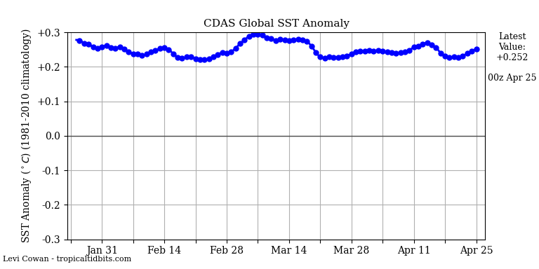
Remarkable since most of it is in the SH.
The basis for understanding weather is that the Earth’s troposphere is very thin, although it protects the surface from extreme temperature spikes. In winter, the height of the troposphere at mid-latitudes can drop to about 6 km, so the stratospheric vortex can interfere with winter circulation.


It was also the warmest 101 months in the UAH record, meaning that long-term temperatures have continued to rise over the duration of the New Pause.
The full warming in UAH TLT up to Aug 2014, the month before the onset of the pause, was +0.39C. After 101 months of ‘pause’, it now stands at +0.59C. An increase of +0.20C during the New Pause.
This is also reflected in the warming rates. Up to Aug 2014 the full warming rate in UAH was +0.11C/dec. It now stands at +0.13C/dec. Funny old ‘pause’.
And because of this we all need to be forced into driving battery cars?
Get real.
You as usual completely missed the point of the article how did you miss the obvious so well?
You forgot to mention that CERES has already explained the warming since 2014. It was caused by solar energy. In fact, the warming was reduced by increases in OLR which was supposed to be going down in your imaginary world.
Richard M said: “You forgot to mention that CERES has already explained the warming since 2014. It was caused by solar energy.”
I think you are referring to Loeb et al 2021 which says:
Note that nearly all of the ASR increase comes from clouds and albedo (figure 2) which the authors say is a response to the warming. In other words, they are confirming the positive feedback effect that has been hypothesized since the late 1800’s.
Loeb also said that it is undeniable that anthropogenic effects are contributing to the EEI and that the Raghuraman et al 2021 study which concluded there is less than 1% chance the EEI is the result of natural internal variability was consistent with his own research.
BTW…I’m not sure Loeb is somewhere the WUWT audience is going to resonate with. Most on here would consider him an alarmist since he has said before that everything you see in the news like fires and droughts are going to get worse if the Earth keeps retaining more and more energy.
You quote an author who spews that kind of nonsensical word salad? When I read the paper I pretty much assumed it was written for morons. No else would do anything but laugh at a paper that use “guesses” as part of their analysis.
Since the clouds have now returned you probably believe that was also “a response to warming”.
No, I was referring to Dubal/Vahrenholt 2021. And the point is that the warming had nothing to do with CO2 despite the idiotic claims from Loeb.
Thank you for your update!
Instead of all the nicky pigging about statistical methods, it would be much appreciated if both Nick and Willis could provide us insight in the “ever increasing?” correlation between the actual Keeling curve and the UAH dataset.
Kind regards
SteenR
In reply to Steenr, correlation does not necessarily imply causation, though absence of correlation generally implies absence of causation. In reality, the divergence between the rate of warming originally predicted and still predicted by IPCC and the observed rate of warming continues to widen.
The pauses tell us that climate sensitivity is on the low end. They show us that there aren’t substantial positive feedbacks.
Aaron is correct. At the temperature equilibrium in 1990 (there was no global warming trend for 80 years thereafter), the absolute feedback strength was 0.22 W/m^2/K. On the basis of the current 0.13 K/decade observed warming trend, the absolute feedback strength remains at 0.22 W/m^2/K. There has been little or no change in the feedback regime since 1850.
Of course, even a very small increase in feedback strength – say, to 0.24 W/m^2/K – would be enough to yield IPCC’s midrange 3 K ECS, or 3 K 21st-century warming (the forcings for these two being about the same). But at current warming rates of little more than 1.3 K/century, there is nothing for anyone to worry about.
Ahh, it’s the Pause that refreshes. But as we all know, the Climate Cacklers, Cluckers, and Caterwaulers have moved on to “Extreme Weather” now because evidently, in addition to CO2’s other powers, it has the remarkable ability to directly affect the weather, and of course, in negative ways.
The Trendology Clown Car Circus cannot abide anything that casts a bad light on CAGW.
Mount Washington (New Hampshire) has reported one of the lowest wind chill temperature ever seen in the United States. A wind chill temperature dropped to -77 °C / -106 °F.
 ?_nc_cat=109&ccb=1-7&_nc_sid=730e14&_nc_ohc=KlJF63sPLHQAX8DKaLb&tn=7LQrPxQelJSA5gda&_nc_ht=scontent-frx5-1.xx&oh=00_AfAzlZUCnitB227v6x67tjU0hDl4GXF99vPs97d34LqGhw&oe=63E44857
Mount Washington (New Hampshire) has reported one of the lowest wind chill temperature ever seen in the United States. A wind chill temperature dropped to -77 °C / -106 °F.
https://www.ventusky.com/?p=44.5;-71.0;5&l=feel&t=20230203/23
CMoB said: “The sheer frequency and length of these Pauses provide a graphic demonstration, readily understandable to all, that It’s Not Worse Than We Thought”
I download the CMIP model prediction data from the KNMI Explorer just now. According to models we should expect to be in a pause lasting 101 months about 18% of the time so the pause we are experiencing now is neither unexpected or nor noteworthy. Interestingly, using a multi-dataset composite (so as not to prefer one over the other) of RATPAC, UAH, RSS, BEST, GISTEMP, NOAAGlobalTemp, HadCRUT, and ERA we see that we have only been a pause lasting that long 15% of the time. So maybe it is worse than we thought. I don’t know.
Exactly how do you extract “pauses” from the CHIMPS spaghetti messes?
More importantly, why do you ascribe any meaning to them?
https://twitter.com/i/status/1614991656583041024
During La Niña, the gobal temperature drops, rather than being constant.
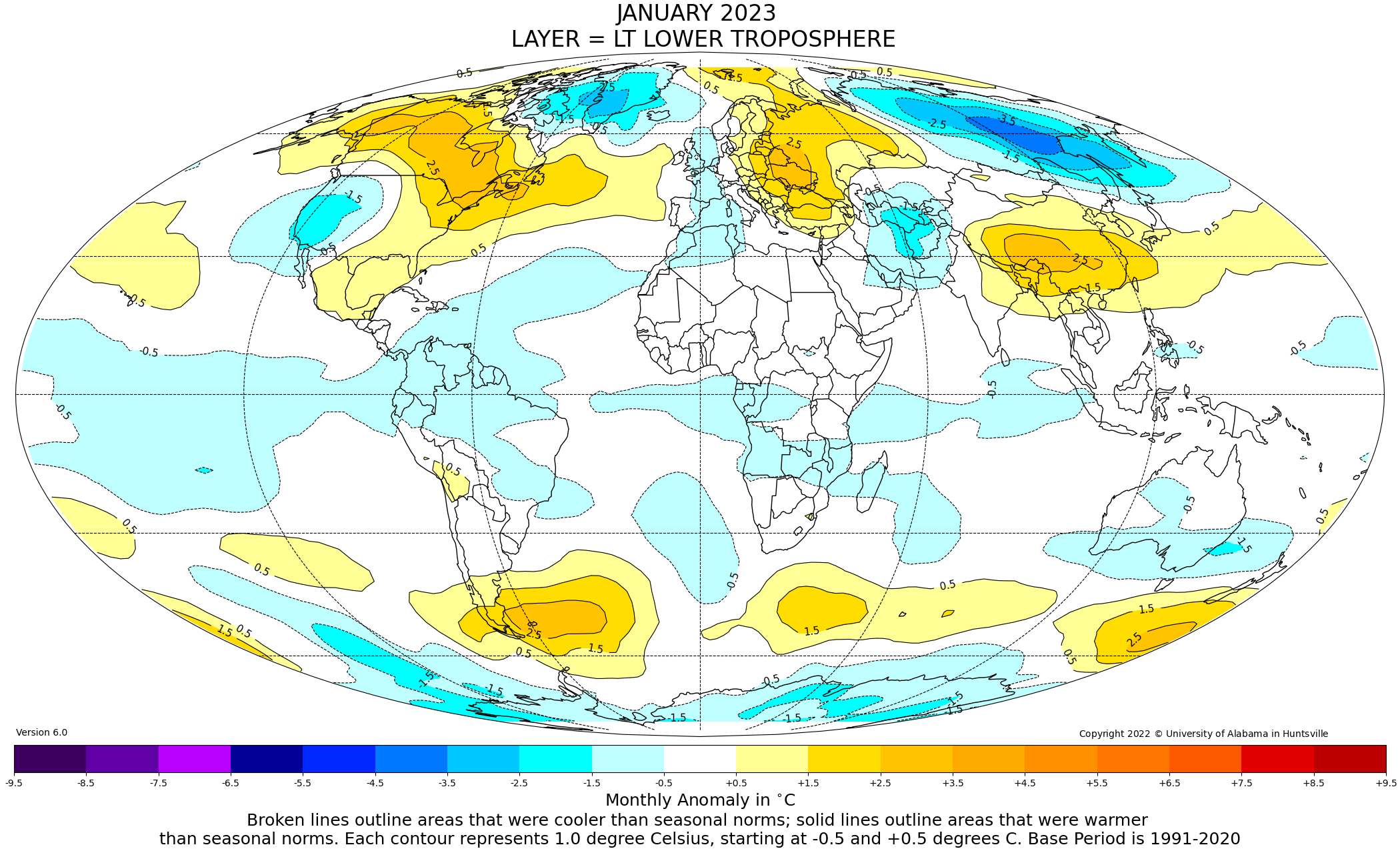
bdgwx February 4, 2023 2:01 pm
Suppose we have two different-sized containers filled with liquid. One liquid has a density of 0.92 kg/l. The other has a density of 1.08 kg/l.
We take them and pour them into a single container. What is the density of the combined liquids?
w.
It is indeterminant given the information. We cannot even always use 1/[(Xa/Da) + (Xb/Db)] because of the microphysical geometry of the substances. Think mixing a vessel of water with a vessel of marbles.
Examples that are deterministic are the Stefan-Boltzmann Law, hypsometric equation, virtual temperature equation, equivalent potential temperature equation, convective available potential energy equation, quasi-geostrophic height tendency equation. the various heat transfer questions, heating/cooling degree day calculations, etc. Obviously statistical metrics like a mean, variance, standard deviation, linear regression, auto regression, durability tests, uncertainty analysis, etc. are examples too.
So you agree that my example shows that it is not valid to perform arithmetic operations on intensive properties?
w.
Absolutely not. Your example only shows that it is invalid in THAT scenario and nothing more.
Do you think the scenarios I listed are invalid?
And BTW…I’m gobsmacked right now because you of all people should know that not only is it possible to perform arithmetic on intensive properties like temperature but it can provide useful, meaningful, and actionable metrics. The SB Law? The analysis you do with CERES data and W/m2 values? The statistics you posted in this very article?
bdg, yes, in certain circumstances you can do arithmetical operations on temperature.
The difference between intensive and extensive variables is that extensive variables vary based on the extent of what is being measured.
Mass, for example, is extensive. If you have twice the volume of a given substance, for example, it will have twice the mass. But temperature is intensive—if you have twice the volume of a given substance, it does not have twice the temperature.
Now, if the extents do not change, then they cancel out of both sides of the equation. This allows us to say, for example, that if we have a liter of a liquid with a density of 0.92 kg/liter and a liter of a liquid with a density of 1.08 kg/liter, when we mix them together we get two liters of a liquid with a density of 1 kg/liter.
The same is true regarding the variation in time of an intensive variable of a given object. Because the extent of the object doesn’t change, it cancels out in the equation and the arithmetic can be performed. So if we measure the temperature of a block of steel over time, we can do the usual arithmetic operations on the time series.
HOWEVER, and it’s a big however, in general my example is true—absent those special situations, you can’t do arithmetic operations on intensive variables.
Best regards,
w.
Strictly speaking, in your example, you won’t necessarily end up with exactly 2 liters.
That is correct. But that was the whole point. Think 1 liter of water mixed with 1 liter of marbles.
I’ll remind you that arithmetic on extensive properties can be abused as well. That doesn’t mean you can’t use arithmetic on extensive properties. Similarly, just because arithmetic on intensive properties can be abused doesn’t mean you can’t use arithmetic on intensive properties.
What I find most disturbing about this is that those who have advocated for the position that arithmetic cannot be performed on intensive properties have performed arithmetic on intensive properties themselves. And when I call them out on it I get a mix of silence, ad-hominems, bizarre rationalizations, incredulity, and/or the mentality “it’s okay for me and my buddies to do it, but no one else is allowed to.”
You miss the point as usual.
First, there is a large difference between using temperature at a single location to determine an average temperature for that location and using geographically separated temperatures to determine average temperatures. Lots of uncertainty when you do that. Station humidities, station environment, station calibration, etc.
Secondly, to use temps as a proxy for heat, one must assume equal humidities, exactly the same station environments, similarly maintained screens, exactly calibrated thermometers, etc.
Averaging disparate stations can only increase uncertainty, it can’t reduce it. It is like control limits in quality assurance. Each separate piece of a product will have a variance from the expected value. One has to take into account individual variances in order to determine the control limits and confidence intervals.
They will refuse to acknowledge that the GAT is not climate until the Moon escapes orbit.
If temperature is an intensive property then the GAT should be the temperature *everywhere*. In essence the GAT is a statistical descriptor which doesn’t describe any reality.
It’ like the average of a 6′ board and an 8′ board being 7′. Where do you go to measure that “average” 7′ board? Does it describe *any* physical reality? Does it help you build a 7′ tall stud wall?
The point they refuse to acknowledge, there is no 7′ board—so bellcurvewhinerman has been reduced to whining about “lumps of wood”.
If the GAT increases/decreases by 0.1 K in a single month, is there a single person on Earth who can notice?
TG said: “If temperature is an intensive property then the GAT should be the temperature *everywhere*.”
I’ll add that to my absurd argument list. I’ll word it as…The average of an intensive property means that it (the average) should be the same value everywhere.
And just so we’re clear I unequivocally think that is an absurd argument. Note that the average of a sample given by Σ[X_i, 1, N] / N does not imply homogeneity or Σ[(X_i – X_avg)^2, 1, N] / (N – 1) = 0.
You forgot to haul out your “contrarian” epithet.
HTH
I assume you agree that temperature is an intensive property, right?
If I average 100F in Phoenix and 100F in Miami and get 100F, then where does that average apply?
Intensive properties are not mass or volume dependent, If you take a 1lb block of steel at 10C and cut it in half, each half will measure 10C.
So if I get an average of 100F above shouldn’t that imply that everywhere between Phoenix and Miami should be 100F? As an intensive property I should be able to cut up the atmosphere between Phoenix and Miami into smaller chunks and find 100F in each chunk.
You keep trying to justify that you can average temperatures just like they are extensive properties.
Do math with intensive properties is perfectly legitimate, e.g. using (t0 – t1), e.g. q = m * C * ΔT.
Saying the average temp of bucket1 of water (10C) and bucket2 of water (6C) is 8C is *not* legitimate. First, you don’t know the amount of water in each (think humidity and temp) so you can’t even accurately determine an average temp if you mixed them. Second, if you don’t mix them then where in between the two buckets can you measure the 6C? If that point doesn’t exist then does it carry any meaning at all?
You certainly don’t get *silence* when you assert things. And you only get ad hominems when you continually assert things that you ‘ve be shown are incorrect. You always cast physical science as “bizarre” when it contradicts what you think are statistical truths that don’t describe reality.
Stop whining.
Not “indeterminant” – indeterminate.
Maybe it is better to say indeterminable?
Jim Gorman February 5, 2023 8:48 am
I truly don’t understand people’s objections to the use of anomalies. An “anomaly” is just the same measurement made with a different baseline.
For example, consider the anomaly measurement that we call the “Celsius temperature”. Celsius temperature is nothing more than an anomaly measurement of Kelvin temperature, with a new baseline set at 0°Celsius = 273.15 Kelvins.
On what planet is this a problem?
w.
The issue is that the baseline, however it is determined via averaging, has its own measurement uncertainty. Subtracting the baseline does not decrease the uncertainty of the original data, it increases it.
What is the uncertainty of the baseline of the Celsius anomaly?
I suggest you’re not talking about an anomaly. I think you might be referring to removing seasonal variations, which is a very different question.
Regards,
w.
Apparently the offset changed by 0.01K in 2019.
According to Wikipedia (so it must be correct)
The uncertainty is determined by “defined as exactly” – there is no uncertainty by definition.
The 273.15K (or 0.16) is an exact value, established by international agreement, it has zero uncertainty. Not unlike how the speed of light now has zero uncertainty, it is exact because of how the meter and second are defined.
The UAH baseline is seasonal because it is composed twelve individual baseline averages, one for each month of the year.
They are an average of 30 years of MSU temperature measurements (in K), and each monthly value clearly has a non-zero uncertainty.
As I said, you’re conflating an anomaly with removing seasonal variations. When you remove seasonal variations you undeniably have uncertainty.
w.
I don’t think I understand the point you are making.
An anomaly is a measurement minus a baseline value. Removing a seasonal variation also requires a subtraction, does it not? Either way, the subtracted value has its own uncertainty that must be treated separately from the measured value.
(The entire UAH processing sequence is much more complex than just one simple subtraction.)
Showing anomalies with accuracy out to the hundredths digit when the underlying components have uncertainties in the tenths digit is just committing measurement fraud.
See the attached graph. It shows most of the anomalies from the models and the satellite records. Most of the values are in the range of 0C to <1C. If the uncertainty of the baseline is +/- 0.5C (which would be the average uncertainty of the baseline components) and the uncertainty of the measurements is +/- 0.3C (probably larger than this) then those uncertainties add for the anomaly. That means that most of the graph should be blacked out since we really don’t know what the actual values are that should be graphed!
It is graphs like this that show the usual narrative from the climate alarm advocates actually is “all uncertainties cancel when doing averages”. “Average values are 100% accurate!”.”
The issue isn’t the use of anomalies. The issue is ignoring what goes along with the use of an anomaly, If there is uncertainty in the baseline value (and there is) and if there is uncertainty in the absolute value being used in the subtraction used to form the anomaly (and there is) then those uncertainties ADD even though you are doing a subtraction.
Anomalies always have higher uncertainties than the components of the anomaly calculation.
It has nothing to do with seasonality (other than the variance of winter temps is higher than that of summer temps implying a greater uncertainty for winter temp data sets).
Averaging doesn’t decrease uncertainty. If adding temperatures into the data set causes the range of values to go up (which means the variance goes up) then the uncertainty of the average goes up as well. Finding an “average uncertainty” only works to spread the total uncertainty evenly across all of the data components, it doesn’t really decrease the uncertainty of the average at all. At the very best, the uncertainty of the average will be that of the data set component that has the highest uncertainty.
That means that the baseline used to calculate an anomaly carries with it the uncertainty of the underlying data components. That uncertainty of the baseline adds to the uncertainty of the anomaly, it doesn’t decrease it.
Monthly anomaly baselines may be useful in removing seasonality effects but they do *NOT* make the results any less uncertain. Anomalies simply don’t give you hundredths digit accuracy if the underlying components of the anomalies have tenths digit uncertainty.
The most absurd aspect of this “climate change” hysteria is the notion that carbon dioxide is a “greenhouse gas” that somehow threatens life on earth. It’s difficult to imagine a greater scientific absurdity. Consider the following:
So, as a professional in time series data analysis who is preparing to give a short course on deterministic and probabilistic models which are intended to characterize and then predict the performance of natural systems I can confidently say something that most of you may already know: it is very important to assess where you start the trend analysis of the data set. As you can see from 1980 to now you would draw an upward trend, from 2015 to now you have a flat or from my point of view somewhat decreasing trend from 2020 on to today. What does that all mean is the real question and to answer that you need a comprehensive understanding of the climate system. Going off on tangents and arguments about the linear regression will get us nowhere. We need valid and verifiable climate models and from my point of view what we have now are nothing more than analytical fantasy.
Excellent. Trends of temperature do nothing but confuse what is going on in the climate. You can not recognize any of the multitude of factors that make up climate.
Climate science has failed much like Chicken Little failed. Temps are rising, temps are rising, we are going to die. The sky is falling, the sky is falling, we are going to die!
We have had over 50 years for science to push for more and better instrumentation of the necessary factors to measure energy, precipitation, various clouds, etc. at different points on the globe. Yet, here we are arguing about the same old thing, temperature! We can’t even get accurate emission measurements of various products.
Willis has given attention to analyzing various parts of the Earth’s climate but when have you seen a paper that tries to gather them under an overarching hypothesis?
It is like everyone is frightened to dig deep for fear of being ran out of town for being a sceptic.
Note that “the full UAH monthly-anomalies dataset since it began in December 1978” reflects global warming only since 1978. Before that year the mean global temperature trend had been downward, which is why several climate alarmists during the 1970s published reports and articles warning about global cooling and a new Ice Age that might be about to start.
dikranmarsupial says at ATTP
February 4, 2023 at 4:53 pm
” Monckton has an algorithm for cherry picking the start point, but it is still cherry picking. His algorithm is selecting the start point that maximises the strength of his argument (at least for a lay audience that doesn’t understand the pitfalls).”
–
DM this is not correct.
ATTP and Willis have used algorithms for most but one of their pauses but Monckton never has.
–
The algorithms incorporating trends are specific to the charts and data used.
One can cherry pick the length of which one of the steps one wants to use,
but, importantly one cannot rig a flat trend.
–
Because Monckton uses a pause, a new pause, this can only go to the end point of the current date and changes from the new date.
Thus he has never selected start point that maximizes the strength of his argument.
The fact that the pause can lengthen or shorten means he has never cherry picked a starting point.
–
Willis, unlike ATTP shows part of a truly long pause from 1997 to 2012.
ATTP breaks it down to two different pauses by incorporating different start and end dates.
Interesting.
I see Monkton has run out of arguments after being shown to be a liar with everything else he’s got to offer.
So this is his 11th hour plea then.
Another cast member of the Trendology Clown Car Circus appears – /yawn/
I couldn’t find anything resembling your claim or data so I went to the source and found this:
https://www.climate.gov/news-features/understanding-climate/climate-change-global-temperature
Earth’s temperature has risen by an average of 0.14° Fahrenheit (0.08° Celsius) per decade since 1880, or about 2° F in total.
The rate of warming since 1981 is more than twice as fast: 0.32° F (0.18° C) per decade.
2022 was the sixth-warmest year on record based on NOAA’s temperature data.
The 2022 surface temperature was 1.55 °F (0.86 °Celsius) warmer than the 20th-century average of 57.0 °F (13.9 °C) and 1.90 ˚F (1.06 ˚C) warmer than the pre-industrial period (1880-1900).
The 10 warmest years in the historical record have all occurred since 2010
If you can send me the actual source of your claim I’d be happy to post that along side the above Actual words from NOAA at climate.gov