Reposted from Dr. Roy Spencer’s Blog
June 19th, 2021 by Roy W. Spencer, Ph. D.
“The magnitude of the increase is unprecedented.”
A new study published by NASA’s Norman Loeb and co-authors examines the CERES satellite instruments’ measurements of how Earth’s radiative energy budget has changed. The period they study is rather limited, 2005-2019, probably to be able to use the most extensive Argo float deep-ocean temperature data.
The study includes some rather detailed partitioning of what sunlight-reflecting and infrared-emitting processes are responsible for the changes, which is very useful. They also point out that the Pacific Decadal Oscillation (PDO) is responsible for some of what they see in the data, while anthropogenic forcings (and feedbacks from all natural and human-caused forcings) presumably account for the rest.
One of the encouraging results for NASA’s CERES Team is that the rate of increase in the accumulation of radiant energy in the climate system is the same in the satellite observations as it is when computed from in situ data, primarily the Argo float measurements of the upper half of the ocean depths. It should be noted, however, that the absolute value of the imbalance cannot be measured by the CERES satellite instruments; instead, the ocean warming is used to make a “energy-balanced” adjustment to the satellite data (which is the “EB” in the CERES EBAF dataset). Nevertheless, the CERES dataset is proving to be extremely valuable, even if its absolute accuracy is not as high as we would like in climate research.
The main problem I have is with the media reporting of these results. The animated graph in the Verge article shows a planetary energy imbalance of about 0.5 W/m2 in 2005 increasing to about 1.0 W/m2 in 2019.

First of all, the 0.5 to 1.0 W/m2 energy imbalance is much smaller than our knowledge of any of the natural energy flows in the climate system. It can be compared to the estimated natural energy flows of 235-245 W/m2 in and out of the climate system on an annual basis, approximately 1 part in 300.
Secondly, since we don’t have good global energy imbalance measurements before this period, there is no justification for the claim, “the magnitude of the increase is unprecedented.” To expect the natural energy flows in the climate system to stay stable to 1 part in 300 over thousands of years has no scientific basis, and is merely a statement of faith. We have no idea whether such changes have occurred in centuries past.
This is not to fault the CERES data. I think that NASA’s Bruce Wielicki and Norm Loeb have done a fantastic job with these satellite instruments and their detailed processing of those data.
What bothers me is the alarmist language attached to (1) such a tiny number, and (2) the likelihood that no one will bother to mention the authors attribute part of the change to a natural climate cycle, the PDO.
So what’s new — the earth has been a greenhouse for 4.5 billion years. And … OMG … it was ice free at least once before. More importantly, no one has ever died from climate change … https://www.youtube.com/watch?v=vaSvvzOPY_Q
I wholeheartedly agree. It would have to be the most protracted death ever recorded.
Now that’s funny. I can just see Hollywood making an epic movie … “Man dies from a 1.5 millimeter flood.”
The irony is that the victim was okay until they applied the 0.3 mm/yr Glacial Isostatic Adjustment.
Good point. I’ll try to get that added to a future video.
“Oh no! I can’t escape the rising ocean. I’m going to drown!!!”
*stands still for 600 years*
Excuse me but a lot of plants and animals have gone extinct over climate change in the 4 billion years of evolution. What you may want to have said is that no one has ever died of ANTHROPOGENIC climate change.
Did you view the 2-minute video?
And 7+ billions have benefited
Pulsar you are the only person I know of that equates the term “no one” to plants or animals.
Doesn’t Evolutionary Theory say that we should be getting more species as the environment changes?
Actually, gazillions of humans have died from climate change, and to claim otherwise is ridiculous.
Most of those deaths due to climate change were due to climate cooling. Crop failures and mass starvation, disease pandemics, human migrations, etc. were direct results of the global cooling experienced in the 16th through mid-19th centuries.. Similarly during the cooling period in the medieval period that ended in the 8th and 9th centuries.
But the number of deaths attributable to global warming is essentially zilch.
More importantly, no one has ever died from climate change
What about the poor Neanderthal during the last glaciation? I’d hate to see how many humans perish during the next glaciation!
Neanderthals died out because they couldn’t outrun us. The climate changes too slow to be the direct cause.
Neanderthals are us. They are human.
Thank you for contributing to the discussion. My general response to your concerns is at the video’s 1:40 minute time point. I especially appreciate your comments about global cooling — which is the real danger in climate change and needs much more attention. I hope others can make videos about this to better educate the public. While I intend to do more myself, this was a start … https://www.youtube.com/watch?v=b1Iu9D5RhqQ&t
That energy inbalance is almost certainly smaller than the measurement errors, That would mean they were graphing noise.
Ignoring measurement error and model error is StOP for climate science these days. Chris.
Pretty much none of what they announce in an AGW context has any physical meaning.
We had a thunderstorm roll through here in the Front Range of Colorado this afternoon and the temperature dropped about 30F in a half an hour. I’m glad the cooling stopped because at that rate all atomic motion would have ceased in about 8 hours.
The rain was very welcome as my rain barrel had become dry about a week ago. Now I can go back to worrying whether it will warm by a degree in the next 50 years.
In-situ measurement uncertainty is pretty low. Loeb et al report 0.77 W/m^2 +/- 0.06 from 2005-2019. Satellite measurements from the net radiation flux is 0.77 W/m^2 +/- 0.48. Yes, CERES data has high measurement uncertainty, but it is still statistically significant. When I convert this into the period 2010-2018 I get right at 0.87 W/m^2 +/- 0.06 for In-situ and 0.87 W/m^2 +/- 0.48 for CERES. This compares to Schuckmann 2020 of +0.87 W/m^2 +/- 0.12. The agreement between Loeb and Schuckmann couldn’t be better. And when I combine the PDFs of these 3 estimates I get +0.87 W/m^2 +/- 0.04. The EEI is significantly larger than measurement error here.
The study abstract says an estimated decadal energy imbalance of 0.5 W/m2 +/- 0.47 W/m2. Damned close to a 100% uncertainty.
That’s 0.5 W/m^2 per decade +/- 0.47 W/m^2 per decade. That’s a trend value you are looking at. It is EEI/decade. The actual EEI values are within the publications itself. In section 2.2, paragraph 2, line 1 the in-situ value is stated as 0.77 W/m^2 +/- 0.06 for 2005-2019. In section 3.1, paragraph 2, line 9 the satellite values are stated as 0.42 W/m^2 +/-0.48 in 2005 and 1.12 W/m^2 +/- 0.48 for 2019. That is 0.77 W/m^2 +/- 0.48 for the 2005-2019 period.
https://ceres.larc.nasa.gov/documents/DQ_summaries/CERES_EBAF_Ed4.1_DQS.pdf
CERES net flux imbalance uncertainty is +/-3.5 W/m2 , the rest is creative accounting.
Yes. That’s right. And notice that the +/- 3.5 W/m^2 figure comes from Loeb et al. 2018. Now read Loeb et al. 2021 to see how they arrive at +/- 0.48 W/m^2 for the period 2005-2019.
Looks to me that you’re quoting Table 6.1, which is the uncertainty relating to a 1°x1° cell (based on Loeb et al). The global uncertainty is much lower. They say
“The linear trend of CERES implies a net EEI of 0.42±0.48 W m-2 in mid-2005 and 1.12±0.48 W m-2 in mid-2019.”
Greg,
I think my earlier comment missed the point, which is that what they call EEI is calculated differently to the EBAF imbalance. They have another paper about that, details in my comment here.
https://wattsupwiththat.com/2021/06/19/new-nasa-study-earth-has-been-trapping-heat-at-an-alarming-new-rate/#comment-3274077
So what I get from what you have stated is that a change of about 1.8 molecules of CO2 per year induces a .05 W/m2 +/- .047 W/m2 per year.
Could you show using E= hf how that happens?
No. I definitely did not say that.
Done properly, your last value should be shown as 0.8 +/-0.5. If you anticipate that the value might be used for subsequent computations, then you might want to include a guard-digit and show it as 0.7[7] +/-0.4[8]. However, the way you are displaying the numbers implies that they are known with greater precision than they actually are.
However, considering the wide variation in measurements, it is highly suggestive that the uncertainties are an underestimate. Are the sigma values stated?
If that is the slope of a trend line, what is the R^2 value of the fit? You claimed that it was significant. What is the p-value?
Uncertainties are additive when calculating a difference, surely.
(1.12 +/-0.48) – (0.42 +/-0.48) = 0.77 +/-0.96
Which means the result in this case is pretty meaningless.
No. They would add in quadrature if independent, so 0.77±0.48√ 2 = 0.77±0.68
But they are probably correlated, so the uncertainty could be a lot less, maybe less than 0.48.
No way.
You have that backwards. Adding in quadrature ends up with the propagated error being smaller than simple addition.
Yes, and so it should. This is elementary stats.
1.12 – 0.42 = 0.8 W/m2. That is the change between the 2005 and 2019 values. The uncertainty on that 0.8 W/m2 value is done via summation in quadrature like Nick said so it would actually be 0.8 W/m2 +/- 0.68. But that is the change from 2005 to 2019 which is different than the average from 2005-2019. I was interested in the average (not the change) because I want to compare it with other averages from other publications.
Loeb et al 2021 use a linear regression model to report the 0.42 and 1.12 +/- 0.48 figures. The nice thing about a linear regression is that the simple average of the endpoints is the same as the average of all the values between those endpoints and which the linear regression was computed. That means I can calculate the average of the sample without actually having the sample because I was given the linear regression slope and endpoints. So what I did was (1.12+0.42)/2 to get 0.77 W/m2 for the average of the period 2005-2019. And since they told us that points on the trendline are +/- 0.48 that means the 0.77 figure is +/- 0.48 as well.
Learn what a Type B uncertainty is.
Using type B uncertainty and what is provided in Loeb et al. 2021 can you tell us what you get for the average EEI in the period 2005-2019 using the model they used to analyze CERES data?
Without a formal uncertainty analysis that adheres to the language and methods in the GUM, the numbers are useless.
Do you come to a different conclusion or not?
I just took another look at the paper. I’m pretty sure Loeb et al. 2021 are saying that each of the 29 observations in figure 1 have an uncertainty of +/- 0.48. If that is the case then the standard error of the mean of the sample is actually 0.48/sqrt(29) = +/- 0.09. And as can be seen the sample is well representative of the population. So if that is true then the figure I cited for the average EEI in the period 2005-2019 of 0.77 W/m2 actually has a far lower uncertainty than +/- 0.48. In support of this I wrote each value for the red dots with +/- 0.05 of error on my side. So using summation in quadrature the total uncertainty on the values I put into excel is sqrt(0.48^2 + 0.05^2) = +/- 0.48. I got a mean of 0.80 W/m2 +/- 0.09 on that. In summary…if anything I grossly overestimated that +/- 0.48 value on the EEI average from 2005-2019. But in my defense I didn’t fully understand until now that the individual CERES observations in the figure are +/- 0.48.
Dave
The importance of the lower value is that it is so close to zero. Having 5% confidence (p value is not stated but let’s assume) that the energy imbalance is less that 30 milliwatts/sq m and that at least some of it is PDO induced (possibly all) shows how meaningless this whole show is.
Consider: how much of a difference in cloud cover in the first five years and the last five years is needed to produce an apparent difference of half a Watt? About 1/2720th.
With with PDO considered responsible for half, say, then a change in cloud cover of 0.02% could explain 100% of the rest of the change without any human effects. And there is still the heat loss variation from ozone changes in Antarctica to consider.
More of your usual BS.
bdgwx
You cannot combine sets of measurements and get a result with an uncertainty that is lower than the original component data sets.
Error propagation is well understood save in the climate alarmist sub-community. Wikipedia is your friend.
The uncertainty about the deep ocean temperatures alone is greater than ±1 degree.
Stop with the false precision.
He’s been told this multiple times in the past, yet keeps forging ahead in his abject ignorance of metrology.
Most of my post was reporting the uncertainties provided by Loeb et al 2021 and Schuckmann et al 2020. The only thing I combined were the 3 PDFs consisting of Loeb-insitu, Loeb-ceres, and Schuckmann-comprehensive. There is a deterministic way of solving the combined the PDF, but I am but a simple man so I used a monte carlo simulation. There is a possibility that my MCS code has a bug, but I’ve checked and double-checked it with other PDFs with a known result and I get the exact same resultant combined PDF so I’m pretty sure it is right. Now, if you think I’ve made a mistake (which happens quite often) I’d be grateful if you could provide the right answer and the method you used to get it.
There you go again, bdgwx. Doing the actual arithmetic. Verboten in these fora…
Hey Rube ….
Not quite correct, your conclusion there.
It could be, but not as a matter of fact, as always the truth.
Actually, as far as I can
make up, the supposed detected energy imbalance in the data is certainly smaller than the error tolerance of the system.
But that does not necessarily mean that such detection in such a given can’t be, or has to be considered as impossible and therefore invalid.
Yes it seems and is tiny, but still possibly real.
And according to Roy,
still the work of these guys has value.
Even Roy seems to realise that the argument of this dected energy imbalance being so tiny,
can not and does not by default invalidate it as non real, or a graphing of noise.
Error tolerance is a very complicated and sophisticated b*tch…
especially when considering high precision analytics.
🙂
cheers
” (1) such a tiny number”
Tiny? Imbalance of 1 W/m2 is enough to heat the atmosphere by 1°C every four months, which we couldn’t sustain for long.
Fortunately the sea has more heat capacity. But still, you actually need to calculate what “tiny” can do.
Go on, I’ll bite. What can tiny do? Do you own a calculator?
The short period studied ends on a freaking double Super El Nino, along with some help from the PDO phase, Nick. Since the satellite-derived atmospheric temperatures are falling towards those values that existed at the beginning of the study period, where are we seeing the result of all this forcing? Lets give CERES and Argo a few more years to work before we declare a climate catastrophe in the making. And one part in three hundred is still tiny, below the measurement uncertainty.
None of this changes the fact that 1 W/m2 imbalance can have very large effect. That isn’t changed by measurement uncertainty, El Nino or whatever. It is about the imbalance you would expect to see at this stage.
I’m sorry, but I don’t have a super computer at my disposal to make the calculations. If I did, I’d make damned sure it didn’t show a tropospheric hot spot and would also tune to get an output ECS figure more in line with observational methods of estimating actual ECS/TCR. The Russians seem to do a credible job of matching observations over the 21st Century. Talk with them.
Let’s see.
255K –> 240 W/m^2
256K –> 244 W/m^2
256.25 –>
So it takes a 4 W/m^2 change to get a 1 degree change.
I get an increase of about 0.35K will give about a 1 watt change at the temperature range we are at. Claiming this is a “very large effect” is being pretty catastrophic in your outlook. Knowing that this is well inside measurement precision, let alone the measurement uncertainty range is pretty much a definition of climate alarmism.
But it all sounds like he knows what he is talking about.
Nick
come on, you are jumping of the bridge. You know better, please just stop.
Loeb et al. 2021 report 0.77 W/m^2 +/- 0.48 for CERES and 0.77 W/m^2 +/- 0.06 for In-situ for the period 2005-2019. Both are above the measurement uncertainty.
The study say a combination of CERES and ARGO techniques yields a decadal 0.5 W/m2 +/- 0.47 W/m2. Argue with them.
The figures I cite are from them. They are the EEI.
What you are referring to is the trend in units of W/m^2/decade. That figure is related to the question of whether the EEI is increasing/decreasing/neutral. Their analysis tells us that we can say with 95% confidence that the EEI is not decreasing and that it is more likely than not to be increasing by at least 0.25 W/m^2 per decade. We cannot eliminate the possibility that the increase is actually 0.97 W/m^2 per decade. This should not be confused with the 2019 EEI of 1.12 W/m^2 as reported in the publication.
So in round numbers you are claiming about a 10 W/m^2 increase over a decade. That calculates out to 257.7K. That would b 2.7K over a century. And if it turns out less than your “most likely” scenario the increase would be far less.
Climate alarmism at its best! You alarmists are getting more and more shrill as actual temperatures get farther and farther from your catastrophic predictions.
No. Loeb et al report the linear regression trend of EEI to be about 0.5 W/m2.decade. That is an increase of 0.5 W/m2 over a decade; not 10 W/m2. Furthermore, this is the EEI. It is not the OLR so it cannot be used in the SB law. BTW…note that the average OLR itself will result in a small rectification error when used the SB law so you have to be careful even when doing that.
I mistakenly said decade I should have said century.
If it is a W/m^2 forcing it certainly can be used in SB to calculate a temperature change. It may not have changed yet but if your saying it won’t then what’s the problem?
You said the possibility exists of a 0.97 per decade change. That is about 10 W/m^2.
Are you saying that they specify that they are using an uncertainty of 2-sigma from a normally-distributed sample?
CERES energy budget uncertainty is +/- 3.5 W/m2 . Their result is rigged.
Greg, you are ignoring the error tolerance of the system.
It is ~5W/m2.
A imbalance detection value @ 1W/m2, it means that the actual real imbalance value in the system at that point is
5+1 = 6W/m2.
So still possible to detect a value of imbalance even when that quantitatively is smaller than the uncertainty value of the given dataset derived from…
But if the imbalance itself is real, in value, where the value is above that of the error tolerance of/in the system.
You may understand now why Nick’s head’s on fire is based and triggered by a so so tiny little thingy.
🙂
cheers
That’s from Loeb et al. 2018. Now read Loeb et al. 2021 for details on how they combined in-situ measurements to constrain CERES measurements over the period 2005-2019.
Yikes. This is the 3rd place I’ve found that I claimed Loeb et al 2021 constrained CERES observations with insitu observations. That is totally incorrect. I just reread the relevant section. The insitu and satellite observations are completely independent. The Loeb et al. 2018 uncertainty is includes the accuracy component. What Loeb et al. 2021 are saying is that CERES is precise. And because their analysis focuses on trends instead of absolute values the uncertainty is lower. My apologies for butchering that.
In order to have any confidence in the precision of a measurement, one normally wants a 2-sigma uncertainty that is at least an order of magnitude smaller than the smallest significant digit. In the instance of the claim for this article, it is difficult to justify even one significant figure. That is, to claim with a straight face that the increase was 0.5, the uncertainty should be equal to or less than 0.05!
Additionally, Nick, modern climate science does not understand the climate system in sufficient detail to calculate what will happen with such tiny perturbations. Anyway, the UN IPCC CliSciFi practitioners still deny that the tropospheric hot spot does not exist. I might listen more to them if they didn’t ignore decades of observations.
Correct there is simply no way to know the relevance of that number and the concept of a trend is stupid given what we are talking about.
Yeah and I can tow the entire planet towards jupiter with a 100watt winch with a huge gear down and an unbreakable steel cable …. stupid calculations are always fun but then you are left with reality which bites.
Nick…
If it happens to be a positive imbalance, Nick.
And neither you or any body else can actually tell at this given stage of such a tiny imbalance being either positive or negative.
By the means applied in consideration of such a detection.
In consideration of the error tolerance of the system, the value of detected imbalance shall be approximate to the value of the error tolerance of the system… before one flirts with idea of concluding the sign of the imbalance.
This find in it’s own does not support in anyway either accumulation of warming or shedding of energy from the system in question… not at this stage.
If it is true, it simply makes a point for consideration, that one of the conditions is actually happening.
Nick,
hopefully you may understand, now,
how cracked up or fracked up your position is or happens to be,
in the prospect of this given circumstantial merit, here, in how it is or happens to be here.
So, Nick, in
the most clear stand, as/and as most head on fire dude to be here as an wannabe alarmist in steroids…
What do you really think about your debil, weak, idiotic taken position about the given of the energy imbalance of this Earth system,
as per the subject matter you engage with!
What is your take now!
ACTUALLY!
Speak, if you can.
What do you think!
cheers
Nick, you can’t multiply a small imbalance over time. If your Xmas tree with 240 lights has reached an equilibrium temperature, then you add one more 1 watt light, it is NOT going to burst into flames in a hundred days due to heat buildup of the additional watt. The Xmas tree simply reaches a new minusculy higher equilibrium temperature a couple of hours after you add the 1 watt bulb.
The Xmas tree is close to ambient temperature anyway. For the Earth, ambient is 3K. The 240 W/m2 makes a difference of about 280K. An extra 1 W/m2 could easily add another 1K. As it has. And it won’t stop there.
10K?
100K?
1000K?
From your downers and your wine
You’re so big
It’s so tiny
Every cloud is silver line-y
The great escape for all of you
Tiny is as tiny do
Tiny is as tiny do
Tiny is as tiny do
Tiny is as tiny do
Nick, if you are so certain the Earth is warming due to rising CO2 could you please explain why outgoing long wave radiation (OLR) is rising not falling as earth warms and worse, it is rising at EXACTLY a rate which matches the claimed thermal sensitivity of Earth (3 Watts/C). That implies zero impact on OLR from CO2 or indeed any other source. Remember the entire AGW thesis is that rising GHG acts as a blanket which reduces OLR which is what causes Earth to warm.
BINGO!
That data based reality seems totally ignored by many.
Sunsettommy, thank god someone gets it! I have asked the question so often and I have never got an answer. I can only assume its because there isn’t one (other than accepting that AGW is busted). Your moniker (editor) suggests to me that you scrutinise posts at WUWT. I have sent a short article to WUWT going into this question in considerably more detail (with references) a couple of times but it was not selected. Is there any point in sending it again?
regards Michael Hammer
I am a Moderator only, the job of selecting and posting articles belongs to Administrators, Anthony and Charles.
Have you tried the SUBMIT STORY link?
I have known for years that when the world is warming then OLWR increases, John Kehr pointed this out showing the CO2 continually falls further behind the warming effect since outgoing rate greatly exceeds the CO2 postulated warm forcing math, it isn’t even close!
All CO2 does is slow down Radiative cooling rate, it doesn’t trap heat at all.
Michael,
Do you have a source for that OLR claim?
Hi Nick; sure do. First reference is the above article itself – the orange plot is labelled “net TOA radiation (CERES)” which is effectively OLR and as it shows OLR has risen 3 watts/sqM
but if you want an independent one try
Decadal Changes of Earth’s Outgoing Longwave radiation
Steven Dewitte * andNicolas Clerbaux remote sensing 2018
https://www.mdpi.com/2072-4292/10/10/1539/htm
which shows exactly the same 3 watts/sqM rise
MIchael,
“First reference is the above article itself”
The graph you refer to is net radiation, not absolute OLR. And it is exactly what AGW would predict. GHGs impede outgoing, so the imbalance increases. Energy is conserved, so it must go somewhere. It goes into warming us, or more particularly, the ocean. The blue is the measure of the heat actually going into the ocean (and melting ice etc). The point of the paper is that they match year by year (approx), even though the nominal uncertainty of the orange is higher.
Eventually, if GHGs stabilise, the oceans will warm in response to the forcing, and OLR will rise to match incoming SW again. The discrepancy will disappear, and the warmer world will be sustained. The greater temperature difference between surface and TOA is what is needed to get the 240 W/m2 through the greater resistance.
Stop thinking in one-dimension.
Mindless heckling.
Is it?
How come you ignored the paper?
Decadal Changes of Earth’s Outgoing Longwave Radiation
Does this Man Made barrier show up .
“NASA’s Van Allen Probes Spot Man-Made Barrier Shrouding EarthHumans have long been shaping Earth’s landscape, but now scientists know we can shape our near-space environment as well. A certain type of communications — very low frequency, or VLF, radio communications — have been found to interact with particles in space, affecting how and where they move. At times, these interactions can create a barrier around Earth against natural high energy particle radiation in space. These results, part of a comprehensive paper on human-induced space weather, were recently published in Space Science Reviews.”
Van Allen Probes Spot Man-Made Barrier Shrouding Earth | NASA
Sunsettommy, thanks for your support.
Amazing Nick; The graph was labelled net TOA radiation. Radiation to where? Can only be down or up and radiation down makes no sense so it has to be radiation to space. OLR is long wave radiation to space. So net radiation to space is somehow different to radiation to space? If GHG’s are reducing it what is increasing the radiation at the top of the atmosphere and why would they be increasing. (more surface radiation escaping, more cloud top radiation, more dark matter radiation (sarc)). Maybe the net refers to radiation that is not long wave? Trouble is there is nothing warm enough at the top of atmosphere to radiate anything but long wave (4-50 micron) in fact nothing in the entire surface/atmosphere is warm enough to radiate below 4 microns significantly. All you do is say its net not absolute with absolutely no explanation and then try to justify it by claiming its what is expected. Please define what makes the difference between net and total. You say GHG impede outgoing but the orange graph shows outgoing is not impeded its increasing – that’s the WHOLE POINT.
Also its surprising that you ignore my second and independent reference. I even went so far as to give to a web address to make it super easy for you to find and peruse – just 1 click. Funny that gives exactly the same data. They don’t say net by the way, they simply say OLR versus time/date.
All your comment after the first brief sentence is simply primary school level thermal transfer science – if you put more heat into a system than you take out it warms, really! I never would have thought of that. Nick we have corresponded on and off both on and off line for years. You know at least a bit of my background, that I have worked as a researcher for a large multinational spectroscopy company in your home state for 40+ years (now retired) and I know you worked for CSIRO. While we always seemed to disagree I have always respected your knowledge and skill. I had hoped for a serious enlightening response from you but I have to say you seriously disappoint me.
Michael
“So net radiation to space is somehow different to radiation to space?”
It is net radiation of all kinds, SW and IR. So net incoming energy flux, which is the important thing. I linked elsewhere to a NASA explanatory page, which also emphasises that the convention is inward flux. You can be sure that NASA’a Loeb et al are following this definition. The page starts
“Earth’s net radiation, sometimes called net flux, is the balance between incoming and outgoing energy at the top of the atmosphere. It is the total energy that is available to influence the climate. Energy comes in to the system when sunlight penetrates the top of the atmosphere. Energy goes out in two ways: reflection by clouds, aerosols, or the Earth’s surface; and thermal radiation—heat emitted by the surface and the atmosphere, including clouds.”
As to the second reference, I don’t know what to make of it. It is published in a “pay for play” journal (MDPI); typically, it seems to be effectively unreviewed:
“Received: 17 September 2018 / Accepted: 21 September 2018 / Published: 25 September 2018”
It seems reasonable, but I would look for confirmation. Anyway, the increase in OLR isn’t 3 W/m2.
I’m sorry to disappoint, but you just have the meaning of the graph wrong. No progress can be made until that is sorted out.
Michael,
I see that the new paper by Loeb et al dos have OLR since 2002 plotted in Fig 2 – they call it ETR, and it is in the middle column. The total range is about 1 W/m2, but up and down, so the net change in those years is about 0.5 W/m2.
In the NASA poster for the Earth’s “energy budget”, they use the bogus total irradiance of 340.1 W/m^2, so I assume everyone else is doing the same. That is an average. The variation is +11.5/-11.3 W/m^2 every single year, simply as a function of the eccentricity of the Earth’s orbit around the Sun. I get an atmospheric temperature rise of 1 deg C/W/m^2 in 85.75 days, somewhat more pessimistic than your number, Nick. We should be seeing a 1 deg C rise in temperature every 7.5 days around January 3rd (perihelion) with the extra insolation…yet somehow the Earth manages to get rid of the extra, and conversely not plunge in temperature at the same rate around July 3rd (aphelion).
Willis Eschenbach’s concepts of emergent phenomena helps explain the amazing stability of the Earth’s climate system. But an alleged 1 W/m^2 (which isn’t detectable, let alone accurately measurable, IMHO) is swamped by the huge annual swings.
Climatologists really seem to have an aversion to using uncertainty ranges, and when they do, they often forget to mention whether they are using 1 or 2 sigma. In some cases, such as with mass balance equations of the Carbon Cycle, it seems that they pull a number out of a hat and call it an “expert estimate.” That leads to such things as estimating the cumulative atmospheric CO2 from anthropogenic land use changes since the beginning of the Industrial Revolution as being 30 +/-45 GT C. That is kind of like saying the value of Pi is 3.1 +/-4.7! It isn’t wrong, other than it suggests that Pi could be negative, but it isn’t very useful for anything practical.
I’m not referring to uncertainty, but to actual variations over time in the known total solar insolation. There is an additional range of +/- 0.34 W/m^2 on a roughly 11 year period due to the Solar cycle. These variations happen – they’re not “uncertainties.” The uncertainties have to be added to them if you want to talk about the pedigree of the numbers we use.
Don’t forget the 2% modulation by the Earth-Sun distance, which is about ±15 W/m2.
In forming uncertainties for a varying an input, an estimate is made for the range of variation and its distribution over the range (uniform, normal, etc.). From these an uncertainty is calculated, then included with the final combined uncertainty for the output quantity.
The Earth-Sun distance is the orbital eccentricity to which I referred.
Maybe someday I will get around to writing an article about the various contributions to uncertainty in the measurements of a variable. However, there are, first off, the random instrumental errors in the measurement at a particular point in time. Measuring the diameter of a ball bearing is a different problem from measuring the average daily temperature!
Then there are autocorrelated variations in the value of a variable over time. If one is reporting on the average value (mean) of a time-varying property, both have to be taken into consideration. The two primary variations in the individual measurements are uncorrelated, so the uncertainties can be added in quadrature. However, the time varying values for a single independent variable are typically autocorrelated, at least over short time periods. Thus, the changes as represented by a probability distribution function are best described by the standard deviation. The SD can be viewed as an uncertainty because the larger it is, the less certain one can be about a future prediction. The best one can typically do is to say it will have a certain probability of being in a certain range that can be summarized as stating a mean with +/- 2 sigma.
From where I sit, they try to minimize uncertainty by ignoring a host of additional error sources, focusing solely on the standard deviations of their averages.
Michael,
Trenberth’s budget is specific. It is a global budget based on annual averages, so eccentricity averages out. And it is for specific years, so the sunspot cycle is fixed. The caption for KT09 Fig 1 said
“Fig. 1. The global annual mean Earth’s energy budget for the Mar 2000 to May 2004 period (W m−2).”
“But an alleged 1 W/m^2 (which isn’t detectable, let alone accurately measurable, IMHO) is swamped by the huge annual swings.”
But it is the usual story; periodic swings don’t go anywhere. Yes, we do have an annual swing of that order, although it is dominated by the land in the NH, whose variability swamps the perihelion effect. But neither is extra heat in the system, and it doesn’t accumulate. This 1W/m2 does accumulate.
“What bothers me is the alarmist language attached…”
It’s all about the message. Everything for the message, nothing outside the message, nothing against the message.
It doesn’t matter how good, bad, logical, or absurd the information or study is.
Still, this is a valuable study that moves science forward. It is unfortunate that alarmists have to bend the propaganda to fit the OMG narrative.
One might say that estimating the number of grains of sand on a beach “moves science forward.” However, the value of such data is highly questionable. I think that Roy was trying to be polite and collegial.
“OMG narrative”
I like it! 🙂
Ever heard of “The Nudge Unit”?
https://chiefio.wordpress.com/2021/06/17/today-out-shopping-in-sheep-afornia/#comment-146559
Following the comments leads to “the nudge unit” has an office in Sydney – and New York among others
This is consistent with Schuckmann 2020 which estimated +0.87 W/m^2 +/- 0.12 from 2010-2018.
It is not consistent with Schuckmann since its abstract says the combined CERES/ARGO decadal change is 0.5 W/m2 +/- 0.47 W/m2. Big difference. Go convince the study authors.
Dave, this is the third time now that you have misrepresented the publication. Though in your defense I truly think it is unintentional. The figure you are citing is the trend in W/m^2 per decade. It is the rate at which the EEI is increasing. It is not the EEI itself which in 2019 is 1.12 W/m^2 +/- 0.48 and over the period 2005-2019 is 0.77 W/m^2 +/- 0.48 as analyzed from the CERES data.
So get your units right. Those you gave disagree.
No they don’t. The units for EEI is W/m^2. The units for the EEI trend is W/m2/decade.
I didn’t even bother reading it because I knew that the only way I would be alarmed, marginally, is how they’re lying harder, but I predicted that 5 or 10 years ago.
Cyber-circular file.
Trenbeth’s “Global Energy Budget” was updated March 2009 to show an imbalance of 0.9w/M² I wonder how that came about, might have gone something like this:
Once upon a time on a bright sunny morning a few years back, Dr. James Hansen was looking at Kevin Trenberth’s iconic “World Energy Budget”

when he choked on his morning coffee because he realized that the darn thing balanced. That’s right, energy in equaled energy out. You see, he’s been saying for some time now that heat energy is slowly building up in Earth’s climate system and that’s not going to happen if the energy budget is balanced.
So he did some fast calculations, snatched up his cell phone and punched in Trenberth’s number.
“Hi Kev, Hansen here, how’s it goin’ with you? Got a minute?”
“Sure Doc, what’s up?”
“Glad you asked. I’ve been looking at your energy budget and it balances, can you fix that?”
“What do you mean fix it, it’s supposed to balance?”
“Kev, listen carefully now, if it balances, heat will never build up in the system do you see where I’m going?”
“Uh I’m not sure, can you tell me a little more?”
“Come on Kev don’t you get it? I need heat to build up in the system. My papers say that heat is in the pipeline, there’s a slow feedback, there’s an imbalance between radiation in and radiation out. Your Energy Budget diagram says it balances. Do you understand now?”
“Gotcha Doc, I’ll get right on it” [starts to hang up the phone]
“WAIT! I need an imbalance of point nine Watts per square meter [0.9 Wm²] for everything to work out right.”
“Uh Doc, what if it doesn’t come out to that?”
“Jeez Kev! Just stick it in there. Run up some of the numbers for back-radiation so it looks like an update, glitz up the graphics a little and come up with some gobbledygook of why you re-did the chart you know how to do that sort of thing don’t you?”
“Sure do Doc, consider it done” [click]
And so here’s the new chart:
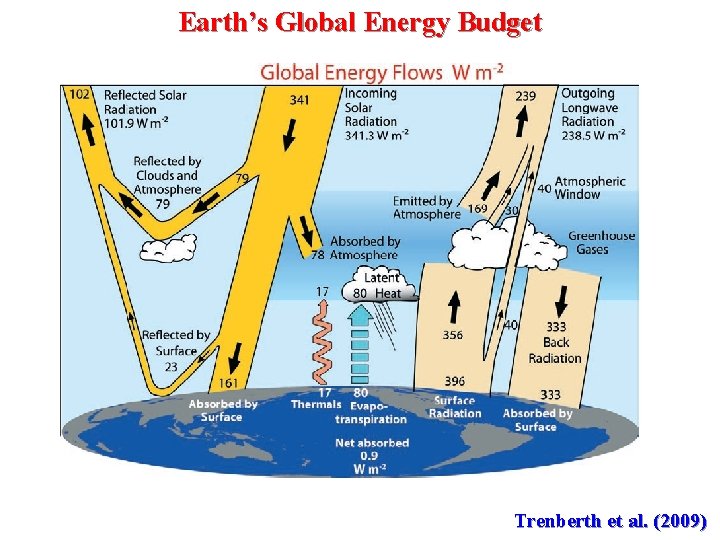
I’ve run the numbers, and 0.9 Wm² will warm the ocean 600 meters deep about 1/2°C in a little over 40 years. Truly amazing stuff. The noon-day sun puts out nearly 1370 wm² and these guys are claiming they’ve added up all the chaotic movements of heat over the entire planet and have determined an imbalance of 0.9 Wm². That’s an accuracy to five places. No plus or minus error bars or anything.
What it means is, all of the components
Reflected by clouds, Reflected by aerosols, Reflected by atmospheric gases, Reflected by surface, Absorbed by the surface, Absorbed by the atmosphere, Thermals, Evaporation, Transpiration, Latent heat, Emitted by clouds, Emitted by atmosphere, Atmospheric Window, AND Back radiation!
need to have an accuracy to those five places or better for the 0.9 Wm² to be true.
Perhaps Hansen didn’t ring up Trenberth and bully him into changing his chart but, Trenberth did change it to show an imbalance and I bet he did so because he realized that if it balanced like his 1997 version, heat wouldn’t build up.
And we all are supposed to sit still for this sort of thing.
The “budget” scam is all the rage in these circles. Saw it with great Rutgers sea level crisis about a week ago.
The simple reason is that there was no measurement of the imbalance in 1997. Now there is.
The claim is that the three main values for Reflected Incoming and Outgoing radiation were measured to those five places. And those three values were changed from the original budget diagram as follows:
Reflected Solar Radiation
101.9 Wm²
was 107 Wm²
Change -5.1 Wm²
Incoming Solar Radiation
341.3 Wm²
was 342 Wm²
Change -0.7 Wm²
Outgoing Longwave Radiation
238.5 Wm²
was 235 Wm²
Change +3.5 Wm²
Difference
0.9 Wm²
was 0 Wm²
So Nick, can the satellites orbiting the Earth measure those three values to five places?
I expect that incoming solar radiation is known to that precision
Source:
https://en.wikipedia.org/wiki/Solar_irradiance
The wikipedia page for Solar radiation was easy to find.
For the other two, not so much.
The solar constant has been decreased by the scientific community from 1366 to 1361 watts per square meter. This over the last 15 years… So multiples of aerosol or CO2 forcings just due to instrument recalibration.
Steve
I basically agree with you, but I only count 4-significant figures, not 5.
Dunno why I typed five
Maybe because you were using 5 fingers on each hand to type? 🙂
IIRC, it was 0.6 W/m2 +/- 17 W/m2 in the Trenberth cartoon I saw a couple of years ago. I could really sink my teeth into that one: There is no way to know what impact Man’s activities have on the massive energy movements in, out and within our climate system.
The EEI is not estimated by adding up all energy transfers. I mean, you could theoretically do it that way, but no one does because that method yields so much uncertainty that it is effectively useless. Instead Trenberth 2009 and others estimate it via the direct heat uptake in the climate system. Trenberth cites an uncertainty on that +0.9 W/m^2 of +/- 0.15.
Explain in laymen’s terms exactly what is measured, and how the uncertainty ( error margins) are calculated.
Also please add in a layman’s description of how Argo is used, and it’s error bars.
And for a bonus, explain how those error bars ( Argo and CERES) interact.
Do the error margins compound?
Of course they compound by Root Sum Square. Again mathematicians never compound either uncertainty or variance between measurements. They obviously are eliminated by averaging, LOL.
Trenberth 2009 uses the Trenberth & Fasullo 2008 method. This is done by measuring the heat uptake in the climate system with a heavy emphasis on the ocean. If I remember correctly they use 1 satellite, 2 reanalysis, and 2 ocean datasets.
I don’t believe ARGO was used.
When I get time I’ll go through the T&F paper and see if CERES substantially improves the measurement. When you have two independent measurements the combined uncertainty is typically just a hair less than the minimum of the two. CERES has a pretty high uncertainty it is unlikely that it improved the overall uncertainty. But then that begs the question…why was CERES used at all? I need to give the T&F publication its due diligence before I comment further.
Where did you learn that two independent measurements have an uncertainty that is the minimum of the two?
Combined uncertainty is done using Root Sum Square. Look it up. Learn some real metrology instead of how to snow people using statistical parameters that have no meaning in uncertainty. If I measure the same thing with two different devices (independent measurements) and then combine them the uncertainty increases. That is, it gets bigger. You can’t even reduce random error by averaging measurements from two different devices. If you don’t believe me find a textbook on measurement error. Even a freshman level will tell you you need measurements of the same thing with the same device in order to eliminate radom error.
No Jim. That is patently false. The uncertainty on a measurable property is no more than the lowest uncertainty of any specific measurement of that property. Adding more measurements of the same thing does not increase the uncertainty. This should be mind numbingly obvious. Think about it. How many times has the distance between Kansas City, MO and St. Louis, MO been measured with a car odometer? Millions? Taking the ever growing sample of odometer readings is the uncertainty on that distance continuing to increase day after day and year after year. NO!
Consider this scenario. If I measure the temperature outside on a hot day based on how much I sweat or feel I might be within +/- 5C if I’m really good and lucky. If I then measure the temperature again with a NIST certificate instrument with +/- 0.5C of uncertainty is the final uncertainty +/- 5.02C or is it +/- 0.5C? Obviously it is +/- 0.5C. Or what if I consult 10 nearby people sweating and ask them based on how they feel and using the same NIST certified instrument? Is the final uncertainty then +/- 15.8C? Nope. It’s still +/- 0.5C. Or what if all 2.5 million people did this in St. Louis today simultaneously and reported their results? Would the uncertainty become +/- 7905C? Nope. It’s still +/- 0.5C.
You use root sum square or summation in quadrature when you are actually adding or combining measurements of different things.
Consider this scenario. If we wanted to know what the diurnal temperature range in St. Louis was today and assuming Tmin/Tmax each have +/- 0.5C of uncertainty then the combined uncertainty is sqrt(0.5^2 + 0.5^2) = +/- 0.71C. We use RSS here because we are adding or combining different measurements of different things. The quantity we are measuring (diurnal range) is dependent on two different measurements of two different things (tmin and tmax).
That is false! The uncertainty will be a hair more than the larger of the two. Look at the example that you gave! sqrt(0.5^2 + 0.2^2) = 0.53 That is NOT just a hair more than 0.2!
When you are justified in using summation in quadrature, it is true that very small errors or uncertainties will have a negligible impact on the result. It will be dominated by the large error(s). Thus, the real impact of quadrature is when all the errors are of similar magnitude. Then it will be different from simple addition, but always smaller.
bd
It does when you are using different devices. The uncertainties most increase when that happens. Here is what I said:
“If I measure the same thing with two different devices (independent measurements) and then combine them the uncertainty increases.”
I followed that up with this statement:
“You can’t even reduce random error by averaging measurements from two different devices.”
If you average the measurements, the uncertainty is is found through RSS. You CAN NOT just assume the uncertainty of the more precise measuring device controls the total uncertainty in an average.
You keep misquoting what I said, why do you do that? You are basically creating straw man arguments which have nothing to add to a discussion.
You also use RSS when combining, and let’s be honest, averaging measurements of different things or measurements using DIFFERENT DEVICES.
The big issue here is that you may use ARGO to validate satellite measurements but you can not use this to reduce uncertainty. That remains an inherent parameter of the device you are using and is unaffected by any other series of measurements by a different system.
No. You do not use RSS when you are averaging measurements of the same quantity. You use the standard error of the mean.
Do a sniff test here. Ask yourself…is what I’m claiming even reasonable on a first principal basis? Do you really think the more times you measure something the more uncertain you are?
Think about a simple scenario to test your claim out. You drive your kid back and forth to school everyday. Let’s say the odometer in your car provides +/- 0.1 miles of uncertainty and that you make 300 trips per year. Do you really think by the end of the 1st year the uncertainty on the distance between your home and the school has grown to +/- 1.7 miles? How about 5 years with +/- 3.9 miles? How about after 13 years with +/- 6.2 miles? And what then after 13 years you hire a surveyor and he finds the door-to-door distance is actually within +/- 0.0001? Do you really think the uncertainty is still +/- 6.2 miles?
Wrong, wrong, and wrong.
This dog you are trying hunt with is quite dead.
Mindless, content-free heckling.
Looks like Nitpick Nick also needs to read the GUM.
Once again you try to build with the same straw Mr Gorman illustrated, and you ignored.
Interesting, curious, persistent, yet remains invalid.
Do you think uncertainty of each measurement, even of the same measurand disappears when you average? Read the following:
Uncertainty of Measurement: A Review of the Rules for Calculating Uncertainty Components through Functional Relationships (nih.gov)
The “standard error of the mean” SEM, is not an estimate of the accuracy nor precision of the measurements. It is an interval within which the mean of the sample means can represent the population mean.
The SEM is an indicator of how accurate the mean is of the “true value” if and only if, the distribution of the multiple measurements of the same measurand is Gaussian and the measurements are independent. In this case the “random errors” can cancel and provide a mean that is a good representation of the “true value”. True value has it’s own definition because ‘uncertainty” can still be large due to systematic error and other biases. In other words, it is no gauge of accuracy.
In all cases, SEM has no bearing on accuracy nor precision. The precision of the measurements can not be increased by finding a mean and calculating statistical parameters about the mean. The numbers are physical measurements, not random numbers on a dice or throws of a coin.
If you read the attached document and the appendices you will learn some of this. I have other references about metrology if you would like them.
Here are three temps, find their uncertainty when the uncertainty of each is 0.5. 21, 28, 35. You may need to read some of the metrology sites. Or you could quote the standard deviation as recommended above.
Straw man argument. But you are calculating the uncertainty on the wrong value. The value is the distance measured Yes, I do think that. Every time you measure the distance ±0.1 miles. For grins, assume it is 5 mi. Then each trip could have an uncertainty of 4.9 to 5.1. Every time you measure it, that uncertainty remains. IOW, two trips would give you 5.8 to 10.2, the third 14.7 to 15.3.
You see uncertainty is what you don’t know, AND CAN NEVER KNOW! Every time you make that trip and write down the mileage YOU DON’T KNOW if it should have been another 4.9 mi or 5.1 mi. It’s not about the number of measurements, it is about the uncertainty in each measurement you take.
If you take a 100 mile trip with that odometer, how many miles do you think you have driven? Is that any different than adding 100 different measurements or 300 measurements?
Here is another question. You may want to consult some surveying texts. If you use a transit that has a ±1 degree uncertainty (±0.28%) and you measure 1 mile (5280 ft) how far off could you be? Do you know how far off you truly are? Does dividing it into 10 pieces help?
No. I definitely do not think the precision of each measurement gets better with more measurements. I never said it. I never implied it. And I don’t want other people to think that either. But I do know that the precision of the mean of the measurements improves with each additional measurement.
Yes. I agree that when you add measurements the uncertainty increases. I don’t agree with how much increases though. You simply added the uncertainty. That’s not correct. When adding measurements you use RSS. So after two trips the total distance now has an uncertainty of +/- 0.14. After 10 trips it is +/- 0.32. After 100 trips it is +/- 1.00. And note that in the context of this post we are not adding different EEI measurements together here so this concept, while interesting, is unrelated.
Your surveying questions is really interesting. I started working on it and quickly realized that it isn’t trivial for a few reasons actually. And I am going to have to refer to surveying texts on it as well.
Here is what you said.
I’ll repeat: “The SEM is an indicator of how accurate the mean is of the “true value” if and only if, the distribution of the multiple measurements of the same measurand is Gaussian and the measurements are independent. It is an interval within which the mean of the sample means can represent the population mean.”
Gaussian and independent are two important qualifies as to how well random errors are offset. IOW, negative values offset positive values and you are left with a “true value”. However, the SEM has no impact on either the accuracy of the instrument nor can it increase the precision of the readings taken by the instrument. If I have a digital meter that has 1 decimal place, I can’t average three or four thousand readings, average them and then say I know the precision out to three or more decimal places. This is why there is a set of rules called “significant digits”. You need to learn them and use them throughout your scientific career.
Simple addition of uncertainties does give you an upper bound on the total uncertainty. You may use quadrature to calculate a possible smaller uncertainty but even that has certain qualifications that you need to be sure is met.
Read Dr. John R Taylor’s book on error to learn about when to use what method.
The question on surveying is very pertinent. If your boss asked you how far off you were what would you say? An accurate answer would be +/- 15 feet but you DON’T KNOW AND CAN NEVER KNOW what the value actually is within that interval.
And if different instruments used for the averaging have different uncertainties, the uncertainty of the average gets even more complex.
Ugh, you really should go read the GUM.
If you have time-series measurements, they are typically autocorrelated. If you have measurements of the same variable with different instruments, they will be correlated. Depending on how you handle them, propagation is probably simple addition rather than addition in quadrature.
Time-series measurements of the same quantity are going to be highly autocorrelated. That’s not an issue. If you are wanting the best estimate of that quantity over that period time you take the mean of the sample. The uncertainty is defined by the standard error of the mean E = σ/sqrt(N). It is not simple addition of E = sum(1…N, σ) nor is it RSS of E = sqrt(sum(1…N, σ^2)). Uncertainty of a quantity does not get worse the more times you measure it.
NO!
This ONLY holds if the same quantity is measured multiple times. In a time- and spatial-series average, NONE of the quantities are identical.
We are talking about the the EEI here. The EEI is a quantity. There are different measurements of it. Each measurement is of the same quantity…the EEI itself. The uncertainty on this quantity is no more than the lowest uncertainty of the sample of measurements available to us. In fact, by utilizing the whole sample of measurements available to us we can actually arrive at a lower the uncertainty. It is the same for the distance between your home and your kids school or a myriad of other quantities. This is an undisputed fact. I’ve read the GUM and it agrees with me on this.
Why did you not respond to my example showing how larger uncertainties control the total uncertainty?
Think about it a moment: If you have two uncertainties being added in quadrature, and the smaller one decreases over time to approach zero as a limit, the limit of the sum will be the larger uncertainty!
What is Eq. 1 (4.1.1) for this EEI number?
You confuse error with uncertainty:
If you read the GUM, you misunderstood what it was saying. Uncertainty when using different devices increases the total uncertainty.
The distance between your kids school and home is an incorrect strawman. If the uncertainty is 0.1 mile, you DON’T KNOW AND CAN NEVER KNOW what the actual value is. No matter how many times you measure it, the uncertainty will remain. If you try to average with another device that has an uncertainty of 0.2, you must use RSS to find the combined uncertainty.
That doesn’t even pass the sniff test Jim. So if a surveyor measures the distance at +/- 0.0001 miles and I measure it with my car at +/- 0.1 then the RSS value is +/- 0.1 miles.
Exactly. Nothing to do with temp, radiation, etc. static. It is always moving so you can never measure the same thing twice. You can’t take a temp today and another tomorrow and average them, and say I know the mean is more both more accurate and/or more precise than either of the components.
I have never seen a “computer programmer” on this web site EVER detail a hard and fast rule about how they decide to stop adding decimal places. Even calculating anomalies breaks significant digits rules every time. You can’t find a base out to two or three decimal places, subtract that from an integer and end up with a 3 decimal place answer. It violates every physical science rule in the book from middle school to doctorate. Do you know how many certified labs would LOVE to do this rather than invest in more accurate and increased precision measuring instruments? Heck, they could use 100 minimum wage folks with 100 triple beam balance scales and report down to the microgram along with uncertainty of 10^-7 precision.
The mean is more accurate and precise as long as the accuracy and precision of each element in the sample is randomly distributed. If it is normally distributed you use the standard error of the mean formula. This is true regardless what dimensionality the measurements embody. Remember, the timestamps of measurements are not a variable in the SEM formula. In fact, the SEM formula doesn’t know either way if the sample even has a temporal or spatial dimensionality to them. Their just numbers. What you do have to be careful about is sampling. The sample must not be biased like might be the case if more observations cluster at the beginning of the time range than the end or other similar problems. For the Loeb et al 2021 mean EEI the samples are well distributed.
Think about the problem using a more canonical and familiar scenario. You want to determine the mean height of all humans at a certain age who have ever lived. You collect a sample from historical records and currently living people. As long as your sampling methodology isn’t biased then the more people you include in your sample the lower the uncertainty of the mean becomes. This is true even though the measurements are of different people at different times and over different parts of the world. The population and sample you select have a temporal and spatial dimensionality to them. This is not a problem. The uncertainty on the mean continues to the decline as your sample size increases.
You didn’t read the GUM nor did you understand it.
A mean of two physical measurements can not be more accurate or precise than the original measurements. A Gaussian distribution of measurements after multiple readings of the same measurand and with the same device will allow the mean to be a good indicator of the “true value” as measured by that instrument.
A mean or average simply can not correct for an inaccurate device. It can not allow you to specify more precision that what was actually measured. It can not reduce the uncertainty of the original measurement. All you are calculating is the accuracy of the mean, not the accuracy or precision of the measurements.
bd is right that you should always be able to get a better estimate from having more measurements. If you take the ordinary mean of two measures u1, u2 with variances V1, V2, then the combined variance is (V1+V2)/2, which is worse then the most accurate, but better than the least.
To get the benefit of the extra information, you need to take the inverse variance weighted mean. That is the weighted mean with minimum variance, which is in fact the harmonic mean V1*V2/(V1+V2). That does have the property of being close to (and less than) V1 if V2 is large, and vice versa.
ONLY when:
4.2.2 The individual observations q_k differ in value because of random variations in the influence quantities, or random effects (see 3.2.2).
4.2.4 For a well-characterized measurement under statistical control, a combined or pooled estimate of variance sp2 (or a pooled experimental standard deviation sp) that characterizes the measurement may be available. In such cases, when the value of a measurand q is determined from n independent observations, the experimental variance of the arithmetic mean q of the observations is estimated better by sp2 n than by s2(qk)/n and the standard uncertainty is u = sp n. (See also the Note to H.3.6.)
Read this web site.
Sampling and Combination of Variables – Statistics and Probability Tutorial (intellipaat.com)
Here is one statement:
Or this:
Combining random variables (article) | Khan Academy
Or this:
AP Statistics: Why Variances Add—And Why It Matters | AP Central – The College Board
Do you see anything in these about dividing by 2 when combining variances? I sure don’t and I have other references if you need them. Perhaps you have a reference of your own.
Also, you need to careful what you are calling populations, samples, population means, and sample means. They all have their own purpose and mixing them all together into a stew just doesn’t work. You can end up with concrete rather than something edible.
“Do you see anything in these about dividing by 2 when combining variances?”
Of course variances add (and it has nothing to do with being Gaussian). So what happens when you take the mean of variable u1, variance V1 and variable u2, variance V2?
m=u1/2+u2/2.
Each variable is scaled and added. What is the variance of u1/2? It is V1/4 (scaling). The variance of u2/2 is V2/4.
So what is the variance of m? It is (V1+V2)/4. Variances add.
Standard error is sqrt(V1+V2)/2.
Do you add the quantities together before finding the average? If so, then you need to calculate the total uncertainty of the sum of the measurements.
Again, the SEM tells you nothing about uncertainty of the measurements. It is only a calculated statistical parameter that indicates the interval which may contain the population mean. It is basically a parameter that tells you how Gaussian your distribution is.
Speaking of SEM, you do realize that is a measure calculated from a sampling of a population. You might explain exactly what sampling is taking place here that allows you to do this. The GUM allows one to quote the SD as an indication of uncertainty. Why don’t you use that?
Jim, it is this simple. If you add measurements you use root sum square (RSS). If you average measurements you use the standard error of the mean (SEM).
See my post to Nick above
You can do it that way too. In fact, that is what Loeb 2021 attempts. But the uncertainty is still pretty high. In fact, Loeb et al. report +/- 0.5 W/m2 of uncertainty with their model as compared to +/- 0.06 W/m2 with the in-situ method. Trenberth 2009 uses the in-situ method by tracking the heat uptake directly. You can review the details in the cited Trenberth & Fasullo 2008 publication.
The precision of the uncertainty is overstated. It should be rounded to 0.2
Trenberth published +/- 0.15. I have no idea where are you getting 0.2.
SIGNIFICANT DIGITS — they should be your friend.
That does not give you the right to change a value that has already been published.
Are you saying that just because something has been set in ink that you would use the value even if it was obviously a typographical error? It probably would warrant a note, but correcting a mistake would be doing the author and science a favor.
In this case, however, it isn’t a typographical error. It is a demonstration that the author is unfamiliar with the proper use of significant figures and rounding of uncertainties to agree with the precision of the mean value.
Exactly, the authors ignored basics of significant digits.
Let’s say the raw calculation Trenberth saw was 0.14679245. What significant digits rule says that we round this value up to 0.2? Why would rounding it to 0.15 violate any significant digits rule here? And if we’re doing to round to 1 significant digit why would you not round down to 0.1 instead?
Let’s say the mean with all digits is 0.89758927 and the uncertainty with all the digits is 0.14679245. How you would round and format for display?
0.9 +/-0.1 If you want to (and can justify) add a guard digit than it would be 0.9[0] +/-0.1[5]
Just because a calculator or spreadsheet give you lots of digits does not mean that they are significant.
I agree. Just because you have a lot of digits does not mean that they are significant or that they should be published. That’s not being challenged. What’s being challenged is the +/- 0.15 uncertainty. Carlo, Monte says it should be 0.2. I’m trying to figure out what the justification is of rounding it like that.
“An introduction to Error Analysis” by Dr. John R Taylor, Professor of Physics, University of Colorado.
Thanks. Yeah, so that document says Trenberth did it exactly right by formatting his figure as 0.9 +/- 0.15 W/m2. Note the rule in 2.5 and note the exception mentioned in paragraph 2 which says “if the leading digit in the uncertainty is a 1 then keeping 2 significant figures may be better”.
This idiotic flat pancake earth energy budget right there is the reason why aliens do not contact you
Exactly! Does anyone here think that 1340 W/m^2 sliding across the earth would cause the same effects as a constant 240 W/m^2? Or would hours of darkness cause the same atmospheric effects as a constant 240 W/m^2?
It is an annual energy budget. Energy is conserved. So yes, you just add up the total energy received.
Averages hide so much.
Energy may be conserved, but to be honest W/m^2 is not a direct measure of energy. This has a time component included that too many people ignore when quoting “energy”.
As I said, the EFFECTS of such widely varying values of power density is what is important. Claiming an average of 33K increase in temperature is based on an average energy figure for a flat earth. What is the increase during the day when 1340 W/m^2 actually hits the earth? Is it still 33K or is it really (1340/240)*(33)=180K? The fact that temperature is used with an exponent means vast differences which is never discussed!
Does convection and water vapor drive more energy toward space when 1340 is hitting the earth that with 240? Averages and means are important to mathematicians working with statistics. That shouldn’t be the case with scientists dealing with real physical phenomena!
Only in the one-dimensional world you inhabit.
“It’s a travesty that we can’t find the missing heat”
– K. Trenberth
(Climategate email)
Well… 341-102 = 239, so it is still balanced. The problem is just how will you get 396 in surface emissions @288K, when surface emissivity is only 0.91?
https://greenhousedefect.com/what-is-the-surface-emissivity-of-earth
Does this model take account of the fact that the Earth is a rotating sphere?
Yes.
Where is this shown in the diagram?
It is shown by the 341 W/m^2 solar input. The solar constant is ~1360 W/m^2. This is the value average over 1 orbital cycle or 366.25 sidereal rotations of Earth. Then you divide by 4 to project it onto a sphere. The energy Earth receives in 366.25 rotations is 341A W-years where A is the area of Earth.
Does it take into account the greater optical path at low solar elevation?
Yes. That is the divide by 4.
Anyone using 240 W/m^2, is not taking rotation into account. It is using an average whose effects are much different than integrals using actual values.
I recommend reading the Trenberth 2009 publication with a particular focus on the section regarding rectification effects. You’ll see that Trenberth is well aware of the spatial and temporal inhomogeneities of all of the figures in the illustration as a result of the diurnal cycle (rotation), albedo, etc. He discusses and even quantifies the error that occurs when you try to estimate the global mean temperature by plugging a global average radiant exitance into the SB law.
Dude, it is more than the “inhomogeneities of all the figures”, don’t you understand that? If I try to heat an ingot with a 100 degree torch and then with a 1000 degree torch do you think the results might be terribly different? How about convection or humidity can they be calculated with an average power density figure?
Steve,
Truer words were never spoken. We are dealing with mathematicians who have no problem using calculations out to the limit of their calculators.
They have never seen this admonition given to new students at Washington Univ. at St. Louis.
“Significant Figures: The number of digits used to express a measured or calculated quantity.
By using significant figures, we can show how precise a number is. If we express a number beyond the place to which we have actually measured (and are therefore certain of), we compromise the integrity of what this number is representing. It is important after learning and understanding significant figures to use them properly throughout your scientific career.
Precision: A measure of how closely individual measurements agree with one another.
Accuracy: Refers to how closely individual measurements agree with the correct or true value.”
These fellows have never heard of significant digits apparently. Nor do they have a clue about precision in measurements. Heck, just divide a couple of numbers and add some extra decimal places to make it look good. No hard and fast rules about when to stop adding precision.
But first you must know the “correct or true value”. Since the starting value of input from sun changes from year to year and season to season etc I think there is is no accuracy in what they measure.
It would be helpful to have the accuracy estimates for CERES and ARGO.
As wonderful as the Argo floats are (and they truly are), their small number in the vast oceans render them a bit player. Not useless, but not significant, either. Add to that the grandiose manipulation of their data to extend its reach the the entire hydrosphere, which discards the actual data and loses information at every step, and one winds up with a mess that obfuscates rather than enlightens.
Once again: The energy budget which is based on the climate model having an atmospheric water amount of only 50 % of the real amount.
If it must be a whole number I prefer +1 rather than -1 W/m2.
Trapping it? Really? Where, up NASA’s a$$?
Roy’s word, not theirs. But it’s true that less heat leaves than arrives.
So, the hockey stick is still a go then?
If that were actually true, the feeback would be run-away.
Perhaps it’s my math skills but I can’t make any formula in this state of imbalance ever come to equilibrium. You seem to want to have your feedback and eat it at the same time. But once you’ve got your imbalanced loop, how do you get rid of it?
Not necessarily. The new system should just balance out at a warmer level than before.
By addressing the source of the additional heat capture.
There is nothing “run-away” in data presented, neither is there any evidence of a feedback.
IF there is currently an imbalance the climate system could change to restore the balance ( for example at a warmer surface temperature ).
Since there are now more polar bears than there were in 2002, and polar bears are proven to be the canary in the coalmine for global warming, it is fair to conclude that the energy budget is negative and the world is cooling.
Not true. Their claimed uncertainty for CERES NET TOA budget is +/- 3.5W/m2
They can not even prove that the imbalance is positive. It’s down in the noise: statistically insignificant change.
The energy imbalance is the difference between incoming solar and outgoing SW+LW.
They bend one uncertainty one, and one the other , to reach the politically required conclusion.
The true uncertainty is far greater than the “imbalance” they are claiming to have found. What they have measured is no statistically significant imbalance and no statistically significant change since 2002.
You have the sense of humor of a dried up dog turd. As to their idiotic claim, if true the Earth’s atmosphere would be like Venus’, yet it ain’t. We are not going to die in a fiery flood no matter how much you environistas wish for it. But hey! Feel whatever you want, it is a free country. Your welcome.
The fundamental questions are why and over what periods has Earth’s energy balance (EEB) has been changing, Nick. Paleo data indicate large changes in the EEB (both positive and negative) over many different timeframes. Instrumental data show large changes (plus and minus) over decadal timeframes. The fact that we can now calculate EEB in the 21st Century does not tell us why EEB went up over such a short timeframe.
An example of the problem is that nobody has rigorously analyzed why we had a Little Ice Age nor why we have been warming coming out of the Little Ice Age. Additionally, why has the globe been cooling for the last few thousand years?
The unknowns of climate abound. Actual observations show that the UN IPCC CliSciFi climate models are bunk. And wild scenarios of future CO2 atmospheric concentrations are risible.
“What bothers me most is the alarmist language ………” Everything these days is perceived with alarm. The safer and the more secure human beings and their civilisation have become – the more alarmed and fearful of everything have they developed : the weather in 100 years – sea-level rise – dying from influenza, etc. -etc.; whoever worried greatly about such in earlier times.
That’s why I contend that civilization is anti-evolutionary. It weakens the species as a whole, as we become more and more dependent on technology and comfortable with its benefits, we become more detached from the harsh realities of nature, and thus end up in a much more precarious position in the face of a disaster.
The Carrington event in 1859 impacted pretty much only communication, its overall impact on society worldwide was almost nothing. A similar event today would set us back farther than where we were in 1859.
The more “civilized” we become, the farther back a major disaster will put us.
“whoever worried greatly about such in earlier times.”
We didn’t have a highly partisan news media promoting all those worries in earlier times.
Now, the Leftwing News Media promotes chaos and division and lawlessness in society, and what do we get? We get chaos, division and lawlessness in our society.
There is a reason for our current situation. The cause is delusional leftwing thinking combined with ownership of Society’s Megaphone, the Leftwing Media. They have created the reality we are now living in, and most of it was created using lies and distortions of reality.
You want to know why things are happening the way they are? That’s why. The Left destroys everything it touches. It’s the nature of the Beast.
The basic findings of the article are important. The climate society has not shown any interest in the fact that there has been a significant increase of SW radiation of 1.68 W/m2 from 2001 to December 2019. Loeb et al. (later Loeb) do not use SW radiation term, but they talk about increased absorbed solar radiation (ASR), which is due to decreased reflection by clouds and sea-ice (the latter being minimal according to my estimate). The SW anomaly of 2001-2020 can explain almost perfectly the temperature ups and downs during this period: link to my web page blog based on the published scientific article: https://www.climatexam.com/single-post/global-temperature-of-april-2021-dropped-below-the-pause-level-of-the-early-2000s
If you compare Figure 1 of my story and Figure 2a of Loeb, you notice that they are identical for SW radiation trend, since they both are direct CERES observations. As you are aware, there has been a strong decrease in the global UAH temperature starting after October 2020: 0.4 °C in October to 0.15 °C in December, to 0.12 °C in January, to -0.01 °C in March, to -0.05 °C in April, and to +0.08 °C in May. This is also in line with the SW radiation changes.
Loeb does not want to address global temperature changes. The reason is that the SW radiation anomaly from 2001 to 2019 has the same magnitude as the CO2 forcing of 1.66 W/m2 from 1750 to 2011 per the IPCC science. According to the climate establishment, natural changes have a minimal role in global warming. Now SW radiation anomaly has shown that they can be very significant indeed.
Better to hide this fact and not to talk about temperature effects. Better to talk about the energy balance effects and the increased OLR value due to the increased greenhouse gases. The latter effect is not due to GH gases, since the present yearly CO2 increase of 2,25 ppm can increase temperature only by 0.02 °C per year. The second reason is that the Earth finds its energy balance very quickly and the increased GH effect does not increase the OLR value: OLR must be the same as incoming SW radiation (=ASR) in about one year time period.
May I suggest something no one seems to have considered?
Given the photosynthetic efficiency of chlorophyll, that 1 watt/m2 is a rough, back of the envelope estimate of the amount of energy doing the useful work of converting sunlight and CO2 into broccoli. The portion of sunlight that goes into sequestering “carbon” that way is not generating heat, and there’s more of that now than in 2005.
I haven’t seen that mentioned on any of the energy balance diagrams, but maybe I didn’t look hard enough.
The Earth is not piled high with broccoli. All the energy consumed in photosynthesis is returned in the subsequent oxidation.
CO2 is greening the planet. That’s stored energy not returned to space.
Indeed, and with a lag; because if CO2 held steady right now, the greening and energy stored in bio growth would continue for a time.
Also, as energy within the system increases, some of that energy could well go into accelerating the hydrological cycle, vs heat.
In general a portion of heat is a waste product of production. The earth system is not 100 percent inefficient.
Sure nick, thats how fossil fuel was formed /sarc
and many of us are very glad that is the case!
Your are right to mention the carbon that is sequestered as a side effect of life. As life increases due to more CO2, the amount of energy naturally sequestered increases.
It’s probably not as much energy as is lost by the enhanced convective water cycle though. The water cycle has multiple effects. It lifts latent energy high into the Troposphere increasing energy loss to space. It creates more clouds especially in the daytime and in the tropics which reflects solar energy. Finally, it leads to less high altitude water vapor which is reduces its contribution to the greenhouse effect.
I saw that headline elsewhere and decided it wasn’t even worth going to as they haven’t even got the records back far enough to prove it.
LOL. Causation is inverted. It’s the stored solar or geothermal that’s raising temperature. The imbalance is a result of internal processes and this warms atmo gases.
Trenberth’s Sankey diagram is an approximation of many readings and calculations for basic explanatory purposes to students. The 0.9 watts is simply calculated from 1.2 degrees global warming since 1850. It is either a complete joke to put it on the chart, or the most accurate W/m^2 number on the chart, depending on your viewpoint….
Splitting a Trenberth type chart into two, one for daytime average and one for nighttime average is an interesting exercise in accuracy considerations.
How can they state there is a “change” if they have no historic data to compare it to?
The timing of the release is pure propaganda. Heat wave that’s currently in the southwest will lead most readers to jump to this being an immediate cause. Just read the headline and it panders to the co2 haters.
Why wasn’t it released while Texas was frozen in February? This smells like opportunistic bull.
It is a cause of the SW heatwave.
also research out this week suggests drought in US worst for 12000 years (and still getting worse).
”research out this week suggests drought in US worst for 12000 years”
Oh I’m sure that’s utterly correct. I mean proxy data is so reliable isn’t it? In fact it’s resolution is so good we should probably use use it for determining how much rain there was 2 years ago.
I looked up that claim and find several news articles- but they all say 1,200 years not 12,000- so, even if it is true – that means you’re off by an order of magnitude, which does not leave me impressed with your perspective. I think you wanted to see 12,000 as it must be more thrilling to you.
In the past century the US southwest has had two droughts that lasted more then one century. Griff’s claim is an absurdity!
You can strike ‘claim is’ without affecting the validity of this statement.
David, your claim is a logical impossibility, or sarcasm.
True, last 1000 years
“Griff’s claim is an absurdity!”
Exactly. Just about all his claims can be described that way.
“It [CO2] is a cause of the SW heatwave.”
Griff says with absolutely no evidence to back up his assertion.
How long do you think the heatwave will last? When the heatwave breaks, and it will, what will have happened to the CO2 that you claim caused the heatwave? Does the CO2 move right along with the high pressure system associated with this heatwave?
CO2, the magic molecule. Griff and Greta see CO2 in everything.
… or while Europe was having one of it longest and coldest springtimes for decades.
Yes, they are getting more desperate! I just read an article today that refined previous speculations that there is a periodicity to geological events. They attributed the change to vulcanism, plate tectonics and CLIMATE!
It should be noted, however, that the absolute value of the imbalance cannot be measured by the CERES satellite instruments; instead, the ocean warming is used to make a “energy-balanced” adjustment to the satellite data
Does this mean they are simply assuming all ocean warming is CO2 caused?
That ignores the fact that upper ocean temperatures have gone up and down like a yo-yo over the Holocene and previously. With no human input and no relation to CO2.
Attribution sleight-of-hand for a pre-determined result.
It’s much more likely all the atmospheric warming is ocean caused. They still have never shown that CO2 increases can warm oceans to any significant degree. However, oceans can warm from multiple causes such as solar spectral variation, cloud changes, increased salinity, microplastic pollution, etc.
The claims of accuracy, both in the paper and in some of the comments here, are overblown. Here’s the real data, from Loeb et al. 2018 (emphasis mine).
So there are two sources of error. First, random errors are the ± 2 W/m2 uncertainty from the calibration, plus the uncertainties from the radiance-to-flux conversion and time interpolation. In addition, we have the bias of the 4.3 W/m2 difference from the calculations based on the standard CERES data products.
This means that the uncertainty in the CERES EEI must be at least ~ 4 W/m2, not ~ half a W/m2 as the authors of the recent study most optimistically claim …
In addition, I’m most suspicious of their “in situ data”. They say:
However, their accuracy claims are … well … let me call them “unlikely”. For example, they claim that:
Seriously? They actually believe they can measure the 13-year change in heat uptake from a “warmer and moister atmosphere” to the nearest 0.009 W/m2? Or the corresponding change in land heat uptake to the nearest 0.004 W/m2?
Sorry, not buying that for one minute. We simply do not have adequate global data to measure heat uptake to that level of uncertainty.
Finally, consider this claim that over 14 years the heat uptake rate is
Now, 0.62 W/m2 is 19.5 megajoules per year, times 14 years is 274 MJ. 2000 cubic metres of seawater is 2047 tonnes. Specific heat of seawater is 3.85 MJ/tonne/°C. So the temperature rise from the heat uptake is 0.035° ± 0.002°C … again, I don’t think we’ve measured the temperature changes of the top 2000m of the ocean to the nearest 0.002°C.
TL;DR version?
No way we can measure the earth’s energy imbalance to that degree of uncertainty, either from satellites or from the ground.
Regards to all,
w.
Thanks for breaking down all these fanciful uncertainties. There is a lot of creative accountancy going on here.
Lies , damned lies and climate statistics.
Also, it is important to remember that the air mass zero irradiance (AM0, at the top of the atmosphere) is modulated by the Earth-Sun distance, which causes the actual value to oscillate by about 2% over course of a single year. In terms of how the solar input is used in climastrology, this should increase the uncertainty by this amount.
Willis,
I think EEI and the imbalance of the CERES-based papers are two different things. In both the Loeb18 and Loeb21 papers, they describe large uncertainties in getting the balance. But that is not their calculation of EEI. The key paper is another by those authors, Johnson16, titled “Improving estimates of Earth’s energy imbalance”. Their they calculate the EEI with low errors, which are cited in the Loeb papers. J16 describe what is going on:
“Earth is gaining energy owing to the addition of greenhouse gasses and the large thermal inertia of the oceans. This gain is difficult to measure directly because it is the small difference between two much larger components of Earth’s energy budget—the amount of incoming solar radiation absorbed and the thermal infrared radiation emitted to space. With over 90% of Earth’s energy imbalance (EEI) being stored in the ocean, the most accurate way to determine it is to measure increases in ocean temperatures (along with increases in land temperatures, decreases in ice mass, and increases in atmospheric temperature and moisture). While the observed net uptake of ocean heat energy is robust over decades, measurement biases and changes in sampling over time have made assessing year-to-year changes difficult.
…
Here, we update our calculations (Figure 1), and find a net heat uptake of 0.71±0.10 W m-2 from 2005.5–2015.5 (with 0.61±0.09 W m-2 taken up by the ocean from 0–1800 m; 0.07±0.04 W m-2 by the deeper ocean4; and 0.03±0.01 W m-2 by melting ice warming land, and a warming and moister atmosphere1). In addition to a remarkable quartering of uncertainty, owing to improved sampling by the Argo array over time (Figure 1), the correlation between year-to-year rates of 0–1800 m ocean heat uptake5 and the latest release of CERES EEI is a much improved 0.78.”
What Loeb 2021 says is that although the absolute uncertainty is high per Loeb 2018 the change uncertainty is relatively low because the instrument is precise even if not accurate. So they anchor or calibrate the CERES data to the insitu observations first.
Hmmm; the most important aspect (at least to me) of this graph is that the net top of atmosphere radiation is increasing. The theory of global warming relies on the claim that GHG’s reduce net energy loss to space – ie: they act like a blanket over earth. Thus more GHG leads to lower energy loss leading to more retained heat which warms the planet. But the data clearly shows the net energy loss to space is NOT DECREASING, it is INCREASING. Seems to me that, all by itself, disproves the theory of AGW. So what is causing the Earth to warm? Looking at NASA data it is increasing absorbed solar radiation and since the solar constant in Earth orbit is indeed constant, that can only come about if Earth’s albedo is reducing. Indeed it is and it appears to be due to reducing cloud cover. The correlation between cloud cover and warming seems pretty good. So how could rising CO2 lead to a reduction in cloud cover? Then on the other hand Svensmark anyone?
It could be because we emit less particulates (less real pollution), so less cloud seeding. Or it could be simply a ‘spontaneous climatic variation’ as Lorenz called it.
Adrian; an interesting reply but I think you sort of missed the point. AGW claims Earth warms because rising CO2 reduces OLR but the experimental data shows OLR is not reducing it is increasing and increasing at exactly the rate predicted by the Stefan Boltzman equation assuming a climate sensitivity of 3 watts/sqM/C which is what is claimed for Earth. That suggests zero impact of rising CO2 on OLR.
Of course the AGW crowd have realised this dilemma and have responded by now claiming that the dreaded feedbacks are causing the absorbed solar radiation (ASR) to rise. Slight problem, feedbacks are a response to an initial change in a parameter but if rising CO2 does not change OLR there is no initial change to drive the feedback. To counter the obvious next stage denial ie: that the feedback drives OLR up but drives ASR up even more, the same comment applies. If there is no net impact on OLR then there is nothing to drive the feedback.
I agree there could be many reasons why albedo is reducing but that is a quite separate issue and nothing to do with the question “is the theory of AGW plausible?”.
How do you interpret a graph labelled as “planetary heat uptake” as clearly shows the “net energy loss to space” is NOT DECREASING, it is INCREASING?
When things appear upside down the first this to do is make sure are holding the paper the right way up.
Greg; the orange plot on the graph in the article is labelled net TOA (top of atmosphere) radiation (CERES) ie: outgoing long wave radiation.
To reply to your comment in the same terms you used “When things appear upside down the first thing to do is make sure you are able and willing to read.”
No, net TOA radiation means net inward flux (SW-OLR). It is defined here.
https://earthobservatory.nasa.gov/global-maps/CERES_NETFLUX_M
If they’re not measuring the entire electromagnetic spectrum they are talking out of their backsides
The CERES page(s) tell me, check yourself, that CERES looks wavelengths between 0.3 microns and 200 microns
Yet Spencer, author and promoter of this garbage, uses data from Sputniks to calculate his Global Monthly temperature – data that is recorded energy coming off the atmosphere at 5 millimetre wavelength
i.e. 5 thousand microns
What is that, wilful blindness, stupidity, lack of knowledge of your own subject – wtf is going on here?
If you want the total actual energy flow, this is The Mistake that Pyrgeometers make, you would look at the colour of Earth.
i.e. You’d put the outgoing energy (all of it) through a spectrometer and the use Wien’s Law to get a temperature and thus calculate a power.
A brave and valid attempt at same was being made in the hand-held IR thermometer Spencer told us about (remember the 42 Celsius cloud, as seen by the man himself from the ground)
But Spencer used a piece of Cheap Chinese Tat (no longer available, surprise surprise) for completely its wrong purpose while perfectly clueless about how it worked and confused it for something off the Starship Enterprise.
Science is going completely backwards – can this ‘End Well’?
Based on these Big Willy Orbiting Trash Cans that
……we are in grave danger of doing something so mind numbingly dumb as to take our own selves down…
any pennies dropping, people?
Esp, that Jozef Stefan is NOT the Be-all and End-all of Climate Science.
(A childlike fixation upon his words might be the End All tho, esp for those too lazy to add an emissivity figure into their calculations)
Basically, we have changed the colour of Earth/earth (farming, tillage, city building, (de) forestry))
All the enrgy is still leaving that came in, just at different frequencies/wavelengths – so where IT All Goes Wrong is in the assumption that nothing has happened, since let’s say, the Mythical & Magical Pre-Industrial Times
Naff example maybe, but a bit like your HiFi Stereo Sound System
We have tweaked the Tone Control – same amount of Total Power going into the speakers, just looks/sounds a bit different.
Remind me, how many different colours can the Human Eye differentiate – there‘s a thinking/starting point for y’all
Reading the actual ‘study’ is painful, it’s pure garbage. Basically it’s used toilet paper. The error bars (the computed ones using tortured statistics, the actual errors are much bigger) are of the same order as the ‘effects’. The confidence intervals are as in cargo cult sciences, very low (95%) and as a consequence such a ‘study’ is almost certainly false (over 6 sigma got to be falsified in physics, ‘certainty’ of three sigma goes away a lot, too). Despite the huge error bars, they have very suspect match between two different methods. That is happening because the data is heavily p-hacked to obtain results conforming with the religious dogma, or because the methods are not really independent (they are really not) or rather, both. They deny physics heavily in the study, claiming that heat is thermal energy and it’s ‘stored’ in the ocean. That’s nonsense. Heat goes in latent heats, too (such as melting the ice or evaporating the water) and also in mechanical work. You also get heat from/into chemical reactions. Denying basic fundamental physics, climastrology 101. Another trick they use is another one stolen from ‘How to Lie with Statistics’: doubling, tripling, increase of a billion times… of a very small value (the ideal value for such claims being… zero). To be noted that the value with a huge error bar also can vary from year to year the same order of magnitude as the entire ‘effect’, so you can get such a ‘doubling’ just by properly cherry picking the start and the end of the numerology. I will reveal what the main conclusion is from the article: it’s the clouds variation. That’s the main contributor. The second one, water vapor, could also be the effect of cloud cover variation. They have no clue on how to correctly simulate those, so they only can do post hoc numerology and claim it science.
CERES documentation claims +/- 3.5W/m2 uncertainty on NET top of atmosphere energy budget. So they cannot even claim that they know energy balance is positive or negative.
their p-value of 0.1 is not impressive, even if it were not a result of p-hacking.
The +/- 3.5 W/m2 uncertainty comes from Loeb et al. 2018. Loeb et al. 2021 uses in-situ observations to constrain the uncertainty further.
Err..my comment here is totally wrong. See my comment here for details.
I invite you all to look full disk midnight infrared sattelite images, then you’ll notice that the big IR radiators are the desert areas.
The nightly minimum temperatures in the deserts are the real indicators of global warming.
See:
Van Wijngaarden, W.A.; Mouraviev, A. Seasonal and annual trends in australian minimum/maximum daily temperatures. Open Atmos. Sci. J. 2016, 10, 39–55.Van Wijngaarden, W.A.; Mouraviev, A. Seasonal and annual trends in australian minimum/maximum daily temperatures. Open Atmos. Sci. J. 2016, 10, 39–55 http://dx.doi.org/10.2174/1874282301610010039
So deserts have a lot less CO2 hanging about?
Seriously, what do deserts lack? Humidity, which allows the IR to radiate out of the atmosphere.
Which is the real thermal blanket?
Good question.
Notice that both Nitpick Nick and bdw-whatever ignored this inconvenient graphic.
The notes on using the CERES data , which explains some of the adjustments and the claimed uncertainly for the various measurements says the uncertainty of the “NET” energy budget measurements are +/- 3.5 W/m2
https://ceres.larc.nasa.gov/documents/DQ_summaries/CERES_EBAF_Ed4.1_DQS.pdf
So in reality, their claimed energy imbalance is statistically insignificant and they can not even state that the imbalance is positive.
Since, as Roy Spencer points out, the two datasets are not independent but CERES is calibrated against ARGO, their entire claim that the two somehow corroborate each other and increase our confidence, is not only incorrect, it is outright deceitful.
The is also the Josh Willis fiasco. When he found ocean cooling in 2006, he was about to announce the finding when he was told to get with the program an fix the data. This resulted in the removal of data from a series of floats which were giving inconveniently low readings. The justification for this post hoc data manipulation was that no similar cooling was seen in CERES.
That further proves that the two datasets agree because they are MANIPULATED to ensure they do agree.
Loeb et al know EXACTLY how these datasets are constructed: it is their own work.
The +/- 3.5 W/m2 figure comes Loeb et al. 2018. Loeb et al. 2021 uses in-situ observations to further constrain the CERES uncertainty. The result is not inconsistent with other estimates of the EEI.
Err…nope. I totally misread the Loeb et al. 2021 paper. They don’t use insitu observations to constrain the CERES uncertainty at all. It is completely independent. What they say is that the Loeb et a. 2018 uncertainty of +/- 3.5 W/m2 is absolute, but the anomaly uncertainty is far lower. In other words, CERES is precise, but not accurate.
A couple of years ago I read in my local paper how climate change was destroying food production. A couple of pages later, farmers were saying it had been the best year ever.
The climate catastrophists show all the traits of psychopaths where controlling people is paramount, especially through fear.
1) It would help more to explain the diagram. For example, is the orange signal “Net TOA Radiation (CERES)” commonly called OLR = outgoing longwave radiation, escaping to space?
If so, their classical model of the greenhouse gas effect makes no sense. James Hansen said:
– Hansen et. al. 2011; Atmos. Chem. Phys. 11, 13421-13449. doi:10.5194/acp-11-13421-2011
Hansen says the climate warming is due to a greenhouse effect lessening escaping OLR energy. The diagram shows more OLR energy escaping over time (with increasing CO2 emissions). Opposite to how Hansen’s model works. The greenhouse gas effect model is clearly nuts. It is logically incoherent. It’s also empirically falsified several times over.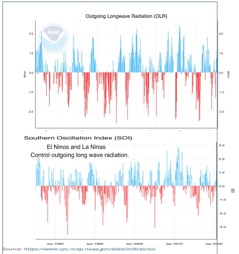
2) Their numbers are subject to massive errors. Such that the error bounds are many times greater than the tiny net signal they claim to see.
3) Their jobs depend on them finding a signal. No signal, no publication, no more grants. It’s not so much the case that they cherry-picked their adjustments to find warming. Although that’s possible. More the case that studies which found cooling, or no warming, never got published; not news-worthy enough.
4) Finally, as the link below shows, The Southern Oscillation Index, SOI, over the Pacific (El Nino & La Nina), determine OLR,
Re: my last point about. This classical greenhouse gas effect model (as explained by Roy Clark elsewhere here), says top of the atmosphere, TOA, radiative imbalance ultimately warms the surface. But the chart I posted shows the surface changes control TOA OLR. Alarmists have inverted caused and effect. They understand things back-to-front.
“the magnitude of the increase is unprecedented.” There is no EXCLAMATION POINT !!!!! at the end of that phrase, thereby diminishing its importance!!!!!!!!!!!!
Aside from attention-seeking behavior and rhetoric, I’m still not sure what these people want. If it’s attention, they are boring me silly, which is why I simply can’t take them seriously. If it’s selling a product, they need to take a look at Iceland, where people are still wearing WINTER clothing in June. You can see that on the live camera sites, when volcano tourists cross in front of those cameras.
And finally, if they’re trying to frighten people with exaggerated language, well – YAWN!!!! Ask them if they’d rather live in perpetual snow and ice and have to hunt for their food. And no, they can’t be veggie-ans in that kind of world, because they’d starve. So would they rather live on a planet that has gone into an ice age? Are they remotely aware that the deserts of this little planet are dreadfully hot daytime, but can and DO drop to freezing cold at night because the air in those places is so dry, there is nothing holding in the heat?
It’s harder and harder to take any of The Them seriously any more. They need to spend some Real Time outdoors, with no bathrooms available, no stores to buy foodstuffs, and shelters they have to set up themselves – and I do not mean camping tents. And watch out for ticks and other nasties, too.
Sara, I agree with your last paragraph completely.
What’s sad is that some of them actually DO spend time outdoors, and still believe their papers and models over what they experienced personally.
And that, TonyG, is SO sad that it is indescribable.
Whatever will they do without a microwave to cook stuff, or a plug-in pot to make hot beverages?
As an engineer I have a good understanding of Thermodynamics and heat transfer including radiation for equipment in pretty much steady state operation, although getting rusty. No experience for the earth’s energy balance
One thing I don’t understand, all the equations I see for energy balance seem to assume this is a steady state process which is OK for most engineering equipment I have experience that might run for 5 years, but not for a process where the sun sets on the earth in “most” places every day and the model does not reflect the actual condition at night when their is no incoming energy from the sun while the earth continues to radiate back to the atmosphere with a portion back radiated to earth, with a gradual cool down absent a weather change . Also this process at every location on earth depends on the time of year, clouds, rainfall and convection.
Can someone explain to me how one creates such a simple steady state model when the actual process is considerably more complex and would require a significantly more extensive calculation procedure as I see it?
It would seem to me that there is considerable uncertainty and variability in the actual factors used to convert the calculations to one temperature (if that is what they do) for the earth and the atmosphere and give lots of opportunity for error and manipulation.
Enlightenment encouraged.
If there is a balance, it’s an extraordinary coincidence. It’s a non-equilibrium system.
Not even in a steady state. There is no thermal equilibrium, no radiative equilibrium, no CO2 equilibrium… and so on. It never was one. They are simply delusional.
It’s a system built on chaos. That is why models don’t really work. There is NO steady state anything, not even water levels, anywhere on this planet.
GCMs are dynamic – no steady state involved.
Something like heating an ingot with 200° torch for an hour, then turning the heat up 5 times to 1000° for a short period. Reckon the effect will just be just the same during the 1000° time as for the average?
This post at NTZ focussing on Gebbie 2021 and some other papers show that global ocean temperatures and changes thereof over the last century are unremarkable. There was three times more heat “trapped” in the oceans during the MWP – or MCA as it’s now called.
https://notrickszone.com/2020/11/05/new-study-effectively-eliminates-confidence-in-human-attribution-for-modern-global-warming/
Yah, no. The atmo has been shrinking in diameter since 2003, it’s an open system that can expand and contract. Atmospheric energy at sea level is regulated by gravity, so unless the air density has been magically dropping in violation of the laws of physics the amount of heat in the atmosphere hasn’t changed.
Meanwhile, another new study shows that Climate Liars have been telling Climate Lies at an alarming new rate.
“Earth has been trapping heat…”
This from NASA, really?
“This from NASA, really?”
They’ve gone off the deep end.
“This from NASA, really?”
No, NASA didn’t say that. The quote is from the Verge article, via Roy.
They said “accumulation”. You are just being pedantically picky, as usual.
According to the TWTW, the abstract claims that the increase is 0.50 +/-0.47 W/m2. It doesn’t state whether that is 1-sigma or 2. Assuming 2-sigma, that means at best, there is a 95% probability that the increase is somewhere between 0.03 and 0.97. Assuming the claimed uncertainty is actually 1-sigma, which is more common for climatology, then it means that there is a 95% probability that the increase ranges between -0.44 and 1.44 W/m2. Both ranges are so large as to make the claim virtually worthless.
However, strictly speaking, when a calculation is shown, it and its uncertainty should be rounded off to show only the digits that share a common uncertainty. Thus, even if the zero is claimed to be significant, the number should be presented as 0.5 +/-0.5. That is, the claimed increase is exactly the same as the uncertainty! That shouldn’t give anyone any confidence in the practical significance of the claim.
Because the data are part of a time-series with obvious auto-correlation, one is not justified in using addition-in-quadrature to calculate the propagation of the uncertainty. That is the one-half watt uncertainty needs to be added to the unspecified starting value uncertainty. We can’t calculate it, but it is going to be larger than 0.5.
CS,
Love seeing an obvious engineer mind in tune with uncertainty and error. You are fully cognizant of and in touch with the physical world as it is. Now compare that to mathematicians who are only in tune with statistics and numbers. Guess who’ll be right in the end!
Jim,
Yes, I have frequently observed that mathematicians are so used to dealing with exact numbers, and non-terminating numbers like Pi and e, that they get cavalier and careless about dealing with uncertainties. Having sat through many a math lecture, the only times I have seen uncertainty discussed was when the chapter topic was was error. Then they promptly forget everything they lectured on because they are focused on process and technique rather than answers.
Most of what I know about uncertainty and propagation of error was learned in physical chemistry classes and the one undergraduate surveying class I took. Dealing with climatology has forced me to review that material.
The 0.50 +/- 0.47 figure is W/m2.decade; not W/m2. It is extremely important to get the units right here.
They do state that the +/- 0.47 figure is 2-sigma. This is in section 3.1, paragraph 2, line 5.