Regular NoTricksZone author Kenneth Richards notes on Twitter
Apparently Arctic sea ice volume was as low in the 1940s as it has been in the 2000s.
And the highest sea ice volume of the last 100 years was about 1979 – the year the Arctic sea ice record begins.🤔

Originally tweeted by Kenneth Richard (@Kenneth72712993) on January 24, 2021.
Here is the complete study published under a CC 4.0 License.
Brief communication: Arctic sea ice thickness internal variability and its changes under historical and anthropogenic forcing
The Cryosphere, 14, 3479–3486, 2020
https://doi.org/10.5194/tc-14-3479-2020
© Author(s) 2020. This work is distributed under
the Creative Commons Attribution 4.0 License.
Guillian Van Achter1, Leandro Ponsoni1, François Massonnet1, Thierry Fichefet1, and Vincent Legat2
- 1Georges Lemaitre Center for Earth and Climate Research, Earth and Life Institute, Université Catholique de Louvain, Louvain-la-Neuve, Belgium
- 2Institute of Mechanics, Materials and Civil Engineering, Applied Mechanics and Mathematics, Université Catholique de Louvain, Louvain-la-Neuve, Belgium
Correspondence: Guillian Van Achter (guillian.vanachter@uclouvain.be) Received: 04 Dec 2019 – Discussion started: 10 Dec 2019 – Revised: 17 Jul 2020 – Accepted: 09 Sep 2020 – Published: 21 Oct 2020
Abstract
We use model simulations from the CESM1-CAM5-BGC-LE dataset to characterise the Arctic sea ice thickness internal variability both spatially and temporally. These properties, and their stationarity, are investigated in three different contexts: (1) constant pre-industrial, (2) historical and (3) projected conditions. Spatial modes of variability show highly stationary patterns regardless of the forcing and mean state. A temporal analysis reveals two peaks of significant variability, and despite a non-stationarity on short timescales, they remain more or less stable until the first half of the 21st century, where they start to change once summer ice-free events occur, after 2050.
How to cite. Van Achter, G., Ponsoni, L., Massonnet, F., Fichefet, T., and Legat, V.: Brief communication: Arctic sea ice thickness internal variability and its changes under historical and anthropogenic forcing, The Cryosphere, 14, 3479–3486, https://doi.org/10.5194/tc-14-3479-2020, 2020.1
Introduction
In the recent decades, Arctic sea ice has retreated and thinned significantly (Notz and Stroeve, 2016). The annual mean Arctic sea ice extent decreased by ∼2×10⁶ km2 between 1979 and 2016 (Onarheim et al., 2018). An analysis combining US Navy submarine ice draft measurements and satellite altimeter data showed that the annual mean sea ice thickness (SIT) over the Arctic Ocean at the end of the melt period decreased by 2 m between the pre-1990 submarine period (1958–1976) and the CryoSat-2 period (2011–2018) (Kwok, 2018). On long timescales (a few decades or more), retreating and thinning are projected to continue as greenhouse gas emissions are expected to rise. However, on shorter timescales (1–20 years), internal climate variability, defined as the variability of the climate system that occurs in the absence of external forcing and caused by the system’s chaotic nature, limits the predictability of climate (Deser et al., 2014) and represents a major source of uncertainty for climate predictions (Deser et al., 2012). In this context, greater knowledge of Arctic SIT internal variability and of its drivers is essential to document the true evolution of the Arctic atmosphere–ice–ocean system and to predict its future changes.
The mean spatial distribution of the Arctic SIT is relatively well documented (Stroeve et al., 2014). But there are some uncertainties around its interannual variability and its spatial modes of variability. Some studies (Lindsay and Zhang, 2006; Fuckar et al., 2016; Labe et al., 2018) already analysed the spatial distribution of Arctic sea ice variability by applying empirical orthogonal functions (EOFs) (K-means cluster analysis for Fuckar et al., 2016) to model-based historical SIT time series. Lindsay and Zhang (2006) reported a first mode nearly basinwide, while the second and third ones are orthogonal lateral modes accounting for 30 %, 18 % and 15 % of the variability, respectively. Fuckar et al. (2016) also found a nearly basinwide first mode, with an Atlantic–Pacific dipole as the second mode. Labe et al. (2018) depicted an Atlantic–Pacific dipole but as the first mode. The spatial structure and amount of explained variance of those modes are sensitive to whether and how the SIT time series is detrended. It is also model-dependent and influenced by the season and analysed period. The temporal sea ice volume (SIV) variability has been studied by Olonscheck and Notz (2017). These authors enlightened a remarkable similarity between the pre-industrial and historical internal variabilities of the annual Arctic SIV. They also noticed a decreased internal variability of winter and summer Arctic SIV for a future climate forced by the RCP8.5 scenario.
Apart from Olonscheck and Notz (2017), the studies cited above used data covering a few decades under historical forcing. In this work we use a long climate model control run under pre-industrial conditions from the CESM1-CAM5-BGC-LE dataset, which enables us to study only the internal variability of the Arctic SIT. We study the internal variability both temporally and spatially by applying a wavelet analysis and an EOF decomposition to the pan-Arctic SIV and gridded SIT anomaly time series, respectively. We also determine whether or not the SIV and SIT variability is stationary by analysing the model outputs under historical and future climate conditions with 30 ensemble members.
This paper is organised as follows. The model and its outputs are briefly described in Sect. 2. In Sect. 3, the spatial and temporal internal variability of Arctic sea ice is analysed, as well as its persistence through historical and future climate conditions. Then we explore the drivers of the main modes of internal variability. Conclusions are finally given in Sect. 4.
2 Data and methods
2.1 Sea ice thickness and volume datasets
We use the CESM1-CAM5-BGC-LE dataset (Kay et al., 2015). The Community Earth System Model Large Ensemble (CESM-LE) was designed to both disentangle model errors from internal climate variability and enable the assessment of recent past and future climate changes in the presence of internal climate variability. The CESM1(CAM5) is a CMIP5 participating model. It consists of coupled atmosphere, ocean, land and sea ice component models. It also includes a representation of the land carbon cycle, diagnostic biogeochemistry calculations for the ocean ecosystem and a model of the atmospheric carbon dioxide cycle (Moore et al., 2013; Lindsay et al., 2014). While it is not possible to validate the data in terms of SIT and SIV variabilities due to the lack of continuous observational data, the model was well validated in terms of mean state of the ice thickness and extent, as well as regarding the recent trends in the latter. Jahn et al. (2016) showed good agreement between observations and CESM1(CAM5) simulations for mean Arctic sea ice thickness and extent in the early 21st century. Barnhart et al. (2016) demonstrated that CESM1(CAM5) captures the trend of declining Arctic sea ice extent over the period of satellite observations. Based on these validation studies, we consider that the CESM1-CAM5-BGC-LE time series is a fair proxy to study the variabilities of the Arctic SIT and SIV under different forcing conditions.
In this paper, we use the monthly averaged Arctic SIT and SIV provided over the three periods (pre-industrial, historical and future). The pre-industrial period is represented by a single 1700-year control simulation with constant pre-industrial forcing. The ocean model was initialised from a state of rest (Danabasoglu et al., 2012), while the atmosphere, land and sea ice models were initialised using previous CESM1(CAM5) simulations. This experimental design allows the assessment of internal climate variability in the absence of climate change. In practical terms, we will use the last 200 years of this simulation. The historical period has one ensemble member covering the 1850–2005 period and 30 ensemble members over 1920–2005. Also with 30 ensemble members, the future climate period (2006–2100) follows the Representative Concentration Pathway (RCP) 8.5 scenario, corresponding to a total radiative forcing of 8.5 W m−2 in 2100 relative to pre-industrial conditions (Meinshausen et al., 2011). The Canadian Archipelago region was removed from the dataset since SIT reaches unrealistic values in this area.
For the variability analysis, the trend and seasonal cycle are removed from the time series (pan-Arctic SIV and gridded SIT) so that we focus on the interannual variability. Since the spatial variability analysis uses 30 ensemble members, the SIT anomaly fields are computed by removing the ensemble mean to each member. When only one ensemble member is used, as for the temporal analysis, the anomaly is calculated by excluding the individual trend (provided by a second-order polynomial fit) of each month.
2.2 Variability analysis
To characterise the internal variability of the Arctic sea ice, we aim at inspecting how the SIV variability evolves in time and how SIT variability is characterised in space. For addressing the temporal variability, we make use of wavelet analysis, with Morlet as wavelet mother, following the methodology proposed by Torrence and Compo (1998). The wavelet analysis has the advantage of taking into account possible non-stationarity of the time series. In this paper, we show the results for one of the historical (1850–2005) members and one of the future (2006–2100) members, although we tested the robustness of the results over the 30 ensemble members as discussed later (Sect. 3.1 and 3.2).
The spatial variability is analysed by computing the EOFs on the SIT anomaly time series. This decomposition reduces the large number of variables of the original data to a few variables, but without compromising much of the explained variance. Each EOF represents a mode of SIT variability that provides a simplified representation of the state of the SIT at that time along that EOF. In other words, the EOFs themselves are fixed in time but their weighting coefficients are time-varying; the associated time series (one for each mode) indicate in which state the SIT is at any time (Hannachi, 2004). The analysis is made on the gridded SIT anomaly time series for the three periods. For the historical and future periods, the EOFs are computed over 30 ensemble members, all appended together over time (as done by Labe et al., 2018).
By applying those analyses separately over the three periods, we aim to document the internal variability in the absence of any external forcing during the pre-industrial period. By comparing the pre-industrial results with those for the historical and future periods, we estimate the evolution of the SIT and SIV internal variability under anthropogenic forcing.
3 Results
3.1 Temporal variability
The results from the wavelet analysis are presented in Fig. 1a–c, in which the wavelet power spectrum is shown as a function of time (bottom left of each subfigure). On the wavelet power spectrum, the crosshatched area denotes the “cone of influence”, in which edge effects become important, and the red lines denote the 95 % significance levels above a red noise background spectrum. The global wavelet spectrum is also shown (bottom right), which is a time-integrated power of the wavelet power spectrum. The significance level of the time-integrated wavelet spectrum is indicated by the dashed curve. It refers to the power of the red noise level at the 95 % confidence level that increases with decreasing frequency.
The temporal variability of the Arctic SIV anomaly over the pre-industrial period is depicted in Fig. 1a. The time-integrated power spectrum (bottom right) shows two peaks of significant variability. The first peak corresponds to a period centred on 8 years but spanning from 5 to 10 years. The second one corresponds to a period of 16 years spanning from 10 to 20 years. In the wavelet power spectrum, the red lines enclose regions in which the variability is significant. The two main peaks are present throughout the time span, but not always concomitantly. Depending on the time, both the 8- and 16-year periods are significant, with one of them appearing stronger in the power spectrum (Fig. 1a, bottom left panel). For instance, the 8-year peak is dominant during the 1780–1810 period, the 16-year peak during the 1750–1780 period and both peaks during the 1830–1850 period.
Over the historical period, the Arctic SIV temporal variability shows a first peak centred on 5 years and two others centred on 10 and 16 years, all with 95 % confidence (Fig. 1b). The wavelet power spectrum shows that the 16-year period is significant throughout the entire time span, while the 8-year period loses significance around certain periods of time (e.g. around 1925). The future climate SIV wavelet analysis in Fig. 1c presents a clear loss of variability after the year 2050. This loss of variability is visible in the SIV time series and is confirmed by both the wavelet power spectrum and the time-integrated power spectrum. The 2050 sudden loss of variability coincides with the ice-free summer events occurring at that time. Apart from that loss of variability, the wavelet power spectrum exhibits one band of 5-year variability during the 2015–2025 period and another band of 10-year variability during the 2025–2050 period, both bands with 95 % confidence. In Fig. 1c, the peaks are not significant on the time-integrated power spectrum because the respective variability is significant only over the first 50 years as is shown in the wavelet power spectrum (areas in red).
The main characteristics of the temporal variability of the Arctic SIV under pre-industrial conditions seem to persist under anthropogenic forcing. The two major temporal peaks of variability centred on 8 and 16 years, found in the pre-industrial run, are also present during the historical period. For the first half of the 21st century, the future projections are also dominated by the two main peaks but centred at 5 and 10 years in the integrated spectrum, and with relatively weaker power compared to the pre-industrial and historical runs. Furthermore, the SIV variability seems to be non-stationary since the power is not always above the 95 % significance level.
The wavelet analyses applied to the other 30 ensemble members of the historical and future simulations bring robustness to our results since, overall, each member shows a similar pattern of temporal variability. To promote such a multi-member comparison among the different spectra, we have first normalised all spectra (and the significance curve) by their respective maximum value so that the power ranges from 0 to 1. This step is required to make the spectrum from each member have the same weight in the averaging. As shown in Fig. 1d (blue line), the averaged spectrum is smoothed out across the time domain because the peaks from different spectra are not co-located exactly at the same periods. Nevertheless, it still shows that the variability is significant over the background red noise (see dashed red line). To complement this analysis, we have counted the number of local peaks for each period and from all 30 spectra. As shown by the black line in Fig. 1d, there is a concentration of peaks around the 8-year and 22-year periods. This spread compared to the reference historical run is somehow expected since the internal variability between the different members is not expected to be identical and even tends to increase with time (Blanchard-Wrigglesworth et al., 2011). For members covering the 21st century, the results are close to the one-member analysis discussed above.
3.2 Spatial variability
The spatial variability of the Arctic SIT anomaly is depicted by the major modes of variability in Fig. 2. Since the SIV exhibits a strong loss of variability around the year 2050, the future period for this spatial variability analysis spans from 2006 to 2050. For each period, the modes are sorted by percentage of variability explained. The first mode, which explains most of the variability, represents 22 %, 20 % and 20 % of the variability for pre-industrial, historical and future climate conditions, respectively. All periods show the same pattern of SIT spatial variability for the first mode. It corresponds to a dipole between the Fram Strait area and the East Siberian Sea (Fig. 2a, b, c). For both the pre-industrial and historical periods, the second mode of variability is a pole centred in the East Siberian Sea, but also spreading into the Arctic Basin (Fig. 2d, e). It accounts for 14 % and 11 % of the variability, respectively. The third mode of variability for the pre-industrial period corresponds to a dipole between the Laptev and Kara seas, on the one hand, and the east coast of Greenland, the Chukchi Sea and Beaufort Sea, on the other hand.

The first mode of SIT is stable over time and stays the dominant mode of spatial variability in all three periods. There are some disparities in percentage explained and in magnitude, which could be explained by the different lengths of the periods. As the first mode, the second mode of SIT spatial variability is persistent in the historical period. For the future climate period, the second mode of SIT variability is no longer persistent. It presents a dipole of variability as the first mode, but the Pacific part of the dipole is larger and no longer located in the East Siberian Sea. The third modes of the three periods (Fig. 2g, h, i) exhibit all different patterns of variability and they are not considered in further analysis.
After 2050, the SIT spatial variability is impacted by the sudden decrease in SIT. EOFs computed over the 2050–2100 period (not shown) exhibit the same pattern of the dipole as the first mode for the 2005–2050 period, but the area of high variability is not the same. The Atlantic part of the dipole is shifted toward the north coast of Greenland, and the Pacific part of the dipole is also reduced near the coast.

3.3 Drivers of the major modes of SIT internal variability
By computing the temporal oscillation between phases of a certain mode of variability, we are able to characterise this mode by low and high indices. In order to find the physical drivers of the SIT modes of variability, we investigate the differences in dynamic and thermodynamic features (sea ice velocity, atmospheric surface temperature) between both phases of the modes. Figure 3a, b show the mean Arctic sea ice circulation over the pre-industrial period by compositing the low (a) and high (b) indices for the first mode of SIT variability. The sea ice drift anomaly associated with the positive and negative phases of the first SIT mode shares similar features with the Arctic Oscillation: a cyclonic anomaly in the Beaufort Gyre, impacting the Transpolar Drift Stream, the Laptev Sea Gyre and the East Siberian circulation, as described by Rigor et al. (2002).
Furthermore, applying wavelet analysis to the associated time series of the first spatial mode of variability indicates that the main periodicity of this mode is centred on 8 years and spans from 5 to 10 years (not shown). This result is suggestive of a link between the first mode of temporal variability of the wavelet analysis and the first mode of spatial variability, and so to the Arctic Oscillation.
We also used the associated time series of the second mode of SIT spatial variability to characterise it by low and high indices. The same analysis over the sea ice velocity is performed for the second mode. For both indices, the sea ice velocity fields are similar. We concluded that the second mode is not dynamically driven. Following Olonscheck et al. (2019) results, which demonstrate that the internal variability of Arctic sea ice area and concentration are primarily caused by atmospheric temperature fluctuations, we investigated the differences in mean surface air temperature anomaly over the pre-industrial period between the low and high indices for both the first and second modes of SIT variability. Two widely different states of surface air temperature are found between indices for both modes (the surface air temperature anomaly for the second mode is depicted in Fig. 3c, d). It appears that the SIT variability and the surface air temperature are associated with each other.
4 Conclusions
In this work, we have analysed the internal variability of the Arctic SIT both spatially and temporally with the CESM1-CAM5-BGC-LE dataset. We conducted wavelet analysis of the pan-Arctic SIV anomaly and EOF decomposition of the gridded SIT anomaly, both over a 200-year control run conducted under pre-industrial conditions. Then, to assess the persistence of the SIT anomaly internal variability under anthropogenic forcing, we performed the same analyses with 30 ensemble members over the historical and future periods.
The temporal analysis of the SIV anomaly internal variability shows two peaks of significant variability. One centred on 8 years, spanning from 5 to 10 years, and another one centred on 16 years, spanning from 10 to 20 years. These two peaks of temporal variability are present in both the pre-industrial and historical periods, as well as in the first half of the 21st century. After that, a sudden loss of variability due to ice-free summer events is found. Furthermore, despite a dominant periodicity over the three periods, the SIV anomaly has been observed to be non-stationary. Indeed, the dominant periodicity of the SIV variability can be centred on either 8 or 16 years, depending on the timescale and period. Wavelet analyses over the 30 ensemble members for the post-industrial period have shown the same behaviour of temporal variability within members, except that the peaks are not always centred in 8 and 16 years but somewhere between 5–10 and 15–26 years, depending on the member.
The spatial analysis of the SIT anomaly internal variability has been applied to the 30 ensemble members and reveals two important modes of variability. The first one is a mode with opposite signs centred in the East Siberian Sea and in the Fram Strait area, accounting for 22 % of the variability in the pre-industrial period. This first mode is a dynamical one, related to the Arctic Oscillation, and persists over all pre-industrial, historical and future periods. Furthermore, this first mode of spatial variability has a temporal variability of 8 years (spanning from 5 to 10 years), corresponding to the first peak of variability found in the temporal analysis. The second mode exhibits a large pole of variation centred on the East Siberian Sea going through the Arctic Basin. It represents 14 % of the variability in the pre-industrial period.
The loss of sea ice in summer starting in 2050 and the strong decrease in SIV in winter during the second half of the 21st century (from 15 to 10×103 km3) strongly modifies the variability of the ice both spatially and temporally. The main modes of spatial variability lose their significance or just disappear after 2050, and the temporal analysis shows a total disappearance of the variability at that time.
This analysis of the Arctic SIT and SIV variability bears some limits. Indeed, our results for the temporal and spatial patterns of variability are based on only one model, and despite the use of 30 ensemble members and a reasonable validation against observations, the model is not perfect. Furthermore, the spatial modes of SIT variability are robust for all the 30 ensemble members, but the temporal analysis shows some dissimilarities between members. Other studies with other model outputs are therefore needed to confirm our conclusion.
Finally, in the context of recent climate changes, predicting sea ice has never been so important. However, to validate and improve our predictions, observational data are crucial. In this sense, our variability analysis of internal SIV and SIT variability might help the development of an optimal sampling strategy, taking into account the selection of well-placed sampling locations for monitoring the SIT and, therefore, the pan-Arctic SIV that are not as well documented as the sea ice extent and area (Ponsoni et al., 2020).
Code availability.
The wavelet analysis is performed with the Waipy module on Python (https://github.com/mabelcalim/waipy, last access: 1 March 2020).
Data availability.
Data can be downloaded from the following source:
https://www.earthsystemgrid.org/dataset/ucar.cgd.ccsm4.CESM_CAM5_BGC_LE.ice.proc.monthly_ave.html
(last access: 1 March 2020). The 30 ensemble members used in this study are the first 30 members (001-030).
Author contributions. GVA, LP, FM, TF and VL designed the science plan. GVA conducted the data processing, produced the figures, analysed the results and wrote the manuscript based on the insights from all co-authors.
Competing interests. The authors declare that they have no conflict of interest.
Acknowledgements. François Massonnet and Leandro Ponsoni are a F.R.S.-FNRS research associate and a post-doctoral researcher, respectively. Guillian Van Achter is funded by the PARAMOUR project which is supported by the Excellence Of Science programme (EOS), also founded by FNRS. We thank the two referees for their very helpful comments on an earlier version of this paper.Financial support.
The work presented in this paper has received funding from the European Commission, H2020 Research Infrastructures (APPLICATE project – Advanced prediction in Polar regions and beyond, grant no. 727862 and PRIMAVERA project – PRocess-based climatesIMulation: AdVances in high-resolution modelling and Europeanclimate Risk Assessment, grant no. 641727).
Review statement. This paper was edited by Michel Tsamados and reviewed by two anonymous referees.
References
Barnhart, K. R., Miller, C. M., Overeem, I., and Kay, E.: Mapping the future expansion of Arctic open water, Nat. Clim. Change, 6, 280–285, https://doi.org/10.1038/NCLIMATE2848, 2016.
Blanchard-Wrigglesworth, E., Bitz, C. M., and Holland, M. M.: Influence of Initial Conditions and Climate Forcing on Predicting Arctic Sea Ice, Geophys. Res. Lett., 38, L18503, https://doi.org/10.1029/2011GL048807, 2011.
Danabasoglu, G., Bates, S. C., Briegleb, B. P., Jayne, S. R., Jochum, M., Large, W. G., Peacock, S., and Yeager, S. G.: The CCSM4 ocean component, J. Climate, 25, 1361–1389, https://doi.org/10.1175/JCLI-D-11-00091.1, 2012.
Deser, C., Philips, A. S., Alexander, M. A., and Smoliak, B. V.: Projecting North American Climate over the Next 50 Years: Uncertainty due to Internal Variability, J. Climate, 27, 2271–2296, https://doi.org/10.1175/JCLI-D-13-00451.1, 2014.
Deser, C., Philips, A., Bourdette, V., and Teng, H.: Uncertainty in climate change projections: the role of internal variability, Clim. Dynam., 38, 527–546, https://doi.org/10.1007/s00382-010-0977-x, 2012.
Fučkar, N. S., Guemas, V., Johnson, N. C., Massonnet, F., and Doblas-Reyes, F.: Clusters of Interannual Sea Ice Variability in the Northern Hemisphere, Clim. Dynam., 47, 1527–1543, https://doi.org/10.1007/s00382-015-2917-2, 2016.
Hannachi, A.: A Primer for EOF Analysis of Climate Data, Department of Meteorology, University of Reading Reading, 2004.
Jahn, A., Kay, J. E., Holland, M. M., and Hall, D. M.: How predictable is the timing of a summer ice-free Arctic?, Geophys. Res. Lett., 43, 9113–9120, https://doi.org/10.1002/2016GL070067, 2016.
Kay, J. E., Deser, C., Phillips, A., Mai, A., Hannay, C., Strand, G., Arblaster, J. M., Bates, S. C., Danabasasoglu, D., Edwards, J., Holland, M., Kushner, P., Lamarque, J.-F., Lawrence, D. , Lindsay, K., Midd Leton, A., Munoz, E., Neale, E., Oleson, K., Polvani, L., and Vertenstein, M.: The Community Earth System Model (CESM) Large Ensemble Project, A Community Resource for Studying Climate Change in the Presence of Internal Climate Variability, B. Am. Meteorol. Soc., 96, 1333–1349, https://doi.org/10.1175/BAMS-D-13-00255.1, 2015.
Kwok, R.: Arctic sea ice thickness, volume, and multiyear ice coverage: losses and coupled variability (1958–2018), Environ. Res. Lett., 13, 10, https://doi.org/10.1088/1748-9326/aae3ec, 2018.
Labe, Z., Magnusdottir, G., and Stern, H.: Variability of Arctic Sea Ice Thickness Using PIOMAS and the CESM Large Ensemble, J. Climate, 31, 3233–3247, https://doi.org/10.1175/JCLI-D-17-0436.1, 2018.
Lindsay, K., Bonan, G. B., Doney, S. C., Hoffman, F. M., Lawrence, D. M., Long, M. C., Mahowald, N. M., Moore, J. K., Randerson, J. T., and Thornton, P. E.: Preindustrial-control and twentieth-century carbon cycle experiments with the Earth system model CESM1(BGC), J. Climate, 27, 8981–9005, doi.org/10.1175/JCLI-D-12-00565.1, 2014.
Lindsay, R. W. and Zhang, J.: Arctic Ocean Ice Thickness: Modes of variability and the Best Locations from Which to Monitor Them, J. Phys. Oceanogr., 36, 496–506, https://doi.org/10.1175/JPO2861.1, 2006.
Meinshausen, M., Calvin, S. J., Daniel, J. S., Kainuma, M. L. T., Lamarque, J.-F., Matsumoto, K., and Montzka, S. A.: The RCP greenhouse gas concentrations and their extensions from 1765 to 2300, Climatic Change, 109, 213–241, https://doi.org/10.1007/s10584-011-0156-z, 2011.
Moore, C. P., Lindsay, K., Doney, S. C., Long, S. C., and Misumi, K.: Marine ecosystem dynamics and biogeochemical cycling in the Community Earth System Model[CESM1(BGC)]: Comparison of the 1990s with the 2090s under the RCP4.5 and RCP8.5 scenarios, J. Climate, 26, 9291–9312, https://doi.org/10.1029/2011JD017187, 2013.
Notz, D. and Stroeve, J.: Observed Arctic sea-ice loss directly follows anthropogenic CO2 emission, Science, 354, 747–750, https://doi.org/10.1126/science.aag2345, 2016.
Olonscheck, D. and Notz, D.: Consistently estimating internal climate variability from climate-model simulations, J. Climate, 30, 9555–9573, https://doi.org/10.1175/JCLI-D-16-0428.1, 2017.
Olonscheck, D., Mauritsen, T., and Notz, D.: Arctic Sea-Ice Variability Is Primarily Driven by Atmospheric Temperature Fluctuations, Nat. Geosci., 12, 430–434, https://doi.org/10.1038/s41561-019-0363-1, 2019.
Onarheim, I. H., Eldevik, T., Smedsrud, L. H., and Stroeve, J. C.: Seasonal and Regional Manifestation of Arctic Sea Ice Loss, J. Climate, 31, 4917–4932, https://doi.org/10.1175/JCLI-D-17-0427.1, 2018.
Ponsoni, L., Massonnet, F., Docquier, D., Van Achter, G., and Fichefet, T.: Statistical predictability of the Arctic sea ice volume anomaly: identifying predictors and optimal sampling locations, The Cryosphere, 14, 2409–2428, https://doi.org/10.5194/tc-14-2409-2020, 2020.
Rigor, I. G., Wallace, J. M., and Colony, R. L.: Response of Sea Ice to the Arctic Oscillation, J. Climate, 15, 2648, https://doi.org/10.1175/1520-0442(2002)015<2648:ROSITT>2.0.CO;2, 2002.
Stroeve, J., Barrett, A., Serreze, M., and Schweiger, A.: Using records from submarine, aircraft and satellites to evaluate climate model simulations of Arctic sea ice thickness, The Cryosphere, 8, 1839–1854, https://doi.org/10.5194/tc-8-1839-2014, 2014.
This should come as no surprise to students of Arctic sea ice fluctuations. The long-established ~60 year cycle of 30 increasing ice years, followed by 30 falling at least since the end of the LIA in the mid-19th century is yet again plainly visible in the thickness graph.
Also on display is the well-known dramatic PDO shift of 1977, which I well recall without understanding its significance at the time.
The late ’30s and early ’40s obviously enjoyed ice conditions similar to this century so far, since the Northern Sea Route was open in summer, then and now. Not just the USSR, but even Germany used it to send aid to Japan.
Around 1975 the AMO was at it’s lowest point
Yes, both oscillations were almost in synch in the late ’70s, for a pronounced climate shift exploited by Marxist academics.
Unsurprising yes but how well does this model correlate with observed real world data? Not to put a downer on things but is this model output robust? Given that the majority of models used in climatology are not fit for purpose, does this one break with the trend?
Very well..
With Arctic Temperatures…
With live evidence of rapid decline before 1940
then rapid growth in the 1970s
Also with DOE data…
And Hanson’s early “before-the-con” data
And HAD4 Arctic sea surface temperatures
I too doubt the reported model run is worth much. I read the paper and thought it pretty convoluted, and it would take a massive amount of work to check it out. I’ll have to leave that to others. But the data fred250 posted looks interesting. Might as well toss the model and just use the data?
Actually I think that the study is very worthwhile if it’s accurate. The evidence posted above does support the model output so I’m definitely reassured. Unsupported model output should be treated with healthy scepticism.
How curious?
It appears that some basement dwelling commenters have downvoted unadjusted historical references…
Apparently, they are not supporters of knowledge, history and observation based science?
It’s a shame we can’t see which anti-reality trollops downvote reality.
Facts and real data are an enema to them !
Here’s a hint. It’s not so much whether a model can hindcast; they can all be tuned to accurately hindcast yet different models can produce divergent future predictions. If you see that any model used the RCP8.5 climate forcing you can be assured that it has no basis. RCP8.5 is one of 4 simple climate forcing models intended to BRACKET future forcings that MIGHT exist in 2100 but not with any estimated degree of likelihood. RCP8.5 is an extremely high 8.5 watt/m^2 of climate forcing that has no basis whatsoever in a prediction of the future CO2 concentration trajectory. It’s a bounding case that was expected to have been discarded by now in favor of more defensible models and has often been used by alarmists to “predict” an impending climate crisis – this despite the fact that RCP8.5 is not a prediction of anything at all.
If you see RCP8.5 you can stop reading and you will not have missed anything.
https://www.carbonbrief.org/explainer-the-high-emissions-rcp8-5-global-warming-scenario
Knowing the one and the other commentator here, we will soon learn, that the paper can’t be true, because of, no idea……because it’s wrong, baseless, cherrypicked…. 😀 😀
The old alarmist fallback position was that even if sea ice has trended upward since 2012, volume was down, is thus no longer tenable, either.
Why more ice is better is not justified, just assumed. The ice that matters to polar bears and their main prey species, ringed seals, is shorefast in the spring, not floes in the summer.
I think the Earth, on the whole, would be better offer with no sea ice – all that extra water to irrigate the world, back to paradise-levels of 8k yrs ago, for example. Why people would prefer a cold, dry planet, just hovering above biosphere collapse is beyond me.
Interesting, I note that Peter Wadhams “End of Ice” doom narrative doesn’t get a mention.
With good reason! May it disappear into the anals of bad science (no not a typo)!
Oh, but it NEEDS to be repeated. The Climate Fascists and all of their useful idiot true believers NEED to be reminded constantly of all their predictions that have not come remotely close to being true upon reaching their “expiration dates,” until that thing called “reality” starts to get through their thick skulls.
This would have come as little surprise to Capt. Henry Larsen, of the RCMP, who sailed the 104-foot, schooner-rigged ship St. Roch throughout the Arctic. He made 20 voyages between 1928 and 1948, being the first to sail the NW Passage, West to East, in 1940. He then sailed the St. Roch from East to West in 1943, taking only 86 days. He followed the more northerly passage back to Vancouver. It’s good to know someone has finally acknowledge what was probably common knowledge back then.
Note: “Only one person had ever sailed a ship through the famed Northwest Passage and that was Norwegian Roald Amundsen in 1903-06, from east to west.”
I was going to mention those sailings–in a wooden boat.
She is preserved in a museum at Kit’s Point in Vancouver Harbour.
Cheers –
I remember when she was hauled out and the purpose built dry dock and display building was built for her. I was a member of the Maritime Museum Society at the time and enjoyed going over her for hours, inch by inch, from stem to stern. A beautiful little ship, built like a tank.
In 1999, the Museum added Jaques Piccard’s Ben Franklin mesoscaphe, also known as the Grumman/Piccard PX-15 designed by him to study the Gulf Stream and sponsored by NASA. Sadly their scientific achievements were over shadowed by Apollo 8.
Rory,
It is worth mentioning that Larson’s 1940 passage involved wintering in the artic since there too much ice for him to do it in a single season. Then in ‘43 he got a bigger engine and so could go faster. All of which suggests that there was more ice in the 40’s than the currently.
Oh, a bigger engine…. roflmao !!!.
Still only capable of a fraction of the speed of modern vessels.
You are JOKING aren’t you !
AND he went through the Prince of Wales Strait, which has been basically impassable most of the current years, even with high speed boats and satellite and drone assistance.
Well, you did manage to get one thing right, Isaac. As Fred mentioned, Larsen took the Southern route and in his own words said;
That was from Larsen’s own account … a very interesting read. I’ll take empirical evidence over contrived modeling every day. There’s nothing like 1st hand observation … none of which suggests there was more ice in the 1940s … just in different places.
Title: The North-West Passage, 1940-1942 and 1944. The Famous Voyages of the Royal Canadian Mounted Police Schooner “St. Roch”.
https://gutenberg.ca/ebooks/larsenh-northwestpassage/larsenh-northwestpassage-00-h-dir/larsenh-northwestpassage-00-h.html
The refit of the then aging St. Roch in Dartmouth NS, January 1944, did indeed include a new engine, with double the hp (to 300) and some other modifications. But as for any noticeable increase in speed, that’s very unlikely. A very heavily built, full displacement hull like hers was unlikely to gain any speed advantage from more power. You might want to look up ‘displacement speed/WL ratio’ . I doubt if a pair of RR Merlins (~ 2000 hp) and twin screws could have increased her speed. It’s the hull shape and displacement that determines a boat’s speed, not the amount of power. The extra power was needed for endurance, reliability and safety.
BTW … I built my own 9 meter gaff cutter from the same material as the St. Roch; Douglas Fir, Australian gum, oak and teak … not more than a mile from where the St. Roch was laid down. I’m only a few short blocks from the same spot as I sit here writing.
Thanks for all the comments about the rugged little RCMP ship St Roch and her intrepid crew.
I posted the following a few years ago.
https://wattsupwiththat.com/2018/08/30/arctic-ice-claims-another-ship-this-time-with-a-sinking/#comment-2444728
The Northwest Passage, the final link of which was discovered by John Rae [of the Clan MacRae] circa 1854, was navigated several times in the 1940’s, when it was clearly WARMER THAN TODAY.
Regards, Allan
https://wattsupwiththat.com/2018/02/26/warm-spike-in-arctic-drives-alarmists-into-alarm-mode-but-theres-no-reason-for-alarm/#comment-2292832
A small wooden ship, the St. Roch, sailed through the Northwest Passage and across the high Canadian Arctic twice, in 1942 and 1944. Try doing that in a small wooden ship today.
These voyages followed soon after the global warming period that ended circa 1940. What was the ice extent and thickness then? Probably less than, or no greater than today.
https://www.vancouvermaritimemuseum.com/permanent-exhibit/st-roch-national-historic-site
THE ST. ROCH – A TRUE CANADIAN ADVENTURE.
Built in British Columbia, named after a parish in Quebec, captained by a Norwegian immigrant, crewed by farm boys from across the country, and helped by the Inuit, the St. Roch was the first vessel to sail the Northwest Passage from west to east (1940-1942), the first to complete the passage in one season (1944), and the first to circumnavigate North America.
One of the only ships in service in the Arctic in the early part of the 20th century, the St. Roch is made of an unusual design of thick Douglas Fir planks reinforced with heavy beams to withstand the ice pressure and an outer shell made of some of the hardest wood in the world, Australian Eucalyptus ‘iron bark’.
Between 1928 and 1954, St. Roch logged tens of thousands of miles crossing and re-crossing the Arctic, acting as a floating detachment of the RCMP in the North. At various times a supply ship, a patrol vessel and a transport, the St. Roch was the only link between the various scattered northern communities. Yet it had not yet accomplished the feat for which it would become famous. For many years, it had been the dream of Captain Henry Larsen to cross the Northwest Passage, just as Amundsen had done for the first time in the Goja in 1903. But time and time again, the dream had to remain a dream.
Finally, with the outbreak of the Second World War and the Nazi invasion of Denmark (Greenland), the opportunity presented itself. Launched on its famous voyage on a secret mission to cross the Arctic during the war, this amazing vessel traveled through treacherous and uncharted waters to cross the Northwest Passage and the High Arctic, with only a small crew of steadfast men who had just their skill, talent and no small amount of luck to rely on. Incredibly, they managed to make the crossing not just once, but twice, and in only 86 days the second time!
Thanks … it’s a story close to my heart, having been a boat builder (especially wooden boats). I’ve followed it since the late ’50s. I recommend Larsen’s own accounts of the voyages (link above). I’ve undoubtedly read your earlier contributions, as I have followed WUWT closely since it was started. I look forward to checking out the links you provided (the maritime museum link I have, LOL, I’ve been a member for half a century). I live five blocks from where the St. Roch was laid down (Burrard Drydock). I walk there almost daily.
<em>”A small wooden ship, the St. Roch, sailed through the Northwest Passage and across the high Canadian Arctic twice, in 1942 and 1944. Try doing that in a small wooden ship today.”</em>
Really? This one made the 310th transit of the NW Passage in 2019:
Tecla-1915.jpg
References please.
No offence Phil, but it takes more than an old photo to constitute evidence.
Larsen took three summers to sail W to E, left Vancouver in June 1940, got trapped by ice at Walker Bay (NWT), he was able to leave in July 1941 and was blocked in by ice in Paisley Bay, He was able to leave in August 1942 and reached Halifax in October.
Nowadays this is possible every summer (covid excepted)
I included his own account of the voyage. I suggest you read it.
Whatever gave you that idea? I can’t even imagine why covid would make the slightest difference. You appear to be very confused about ice conditions in the Arctic.
Larsen in the St Roch made the 2nd and 3rd transits of the NW Passage, the 4th transit was by an ice breaker 10 years later (1954). The 10th transit was in 1969, by 2019 there were 300 further transits, many by yachts, the Tecla (a ketch) made the 311th transit in 2019. There are about ten transits per year.
Whatever gave you that idea? I can’t even imagine why covid would make the slightest difference. You appear to be very confused about ice conditions in the Arctic”
Because of COVID restrictions were placed on access to the Passage to prevent the virus reaching the villages in the region. Last summer a sailor ignored the rules and apparently completed the transit (took him 37 days), he was followed by a Canadian navy ship to ensure that he didn’t make contact with indigenous populations. The confusion appears to be yours.
I understand that you’re still somewhat confused. I still suggest you read Larsen’s own account. Covid has nothing to do with whether a Northwest Passage transit is possible. You’re comparing apples to oranges.
There is no single NWP. It varies from year to year … and no, there isn’t a route open every year. Only modern navigational aids have allowed so many transits through the seven main routes.
The NWP will never be a practical link between oceans because winds and currents determine where the ice will be during Summer.
No it isn’t. Some summers in this century the southern route is closed; others the northern. At times both are closed. Please cite the years during which both NW Passage routes have been open.
Thanks!
Another hole blown in the hockey stick
Such a stupid, easily refutable concept
Sadly, also an easy to believe load of crap for the numbskulls….including the vacant media buffoons. It’s interesting how much the media admire themselves…and how despised they are by thinking people. Maybe even more than politicians now. And that makes sense as they spout the same bullshit and for the same mindless reasons. They are little more than a propaganda outlet now….as you all know. Sickening, aint it?
It played straight to the preconceived biases of certain groups. That it was completely wrong didn’t seem to matter in the slightest. More and accurate information about natural climate change will undermine the climate fear machine but we’ll still be stuck with small groups who are divorced from reality.
Related to this is a trivia question.
In what winter did lake superior freeze all the way across?
“We use the CESM1-CAM5-BGC-LE dataset (Kay et al., 2015). The Community Earth System Model Large Ensemble (CESM-LE) was designed to both disentangle model errors from internal climate variability and enable the assessment of recent past and future climate changes in the presence of internal climate variability. The CESM1(CAM5) is a CMIP5 participating model. It consists of coupled atmosphere, ocean, land and sea ice component models. It also includes a representation of the land carbon cycle, diagnostic biogeochemistry calculations for the ocean ecosystem and a model of the atmospheric carbon dioxide cycle (Moore et al., 2013; Lindsay et al., 2014). While it is not possible to validate the data in terms of SIT and SIV variabilities due to the lack of continuous observational data, the model was well validated in terms of mean state of the ice thickness and extent, as well as regarding the recent trends in the latter. Jahn et al. (2016) showed good agreement between observations and CESM1(CAM5) simulations for mean Arctic sea ice thickness and extent in the early 21st century. Barnhart et al. (2016) demonstrated that CESM1(CAM5) captures the trend of declining Arctic sea ice extent over the period of satellite observations. Based on these validation studies, we consider that the CESM1-CAM5-BGC-LE time series is a fair proxy to study the variabilities of the Arctic SIT and SIV under different forcing conditions.”
So a CMIP5 AOGCM/ESM numerical model or 100% numerical model data and it is only a ‘fair proxy’ for anything including SIT, SIV, SIA/SIE. No real accurate observational data at all prior to 1979 and even there we are limited to SIA/SIE.
The only constant here is the inconsistencies of those that on the one hand totally reject numerical climate models and on the other hand fully accept numerical climate models without question. Cognitive dissonance much.
No kidding, I laugh when alarmists says today’s ice is slushy and not like real ice 😜
Yes, of course! It’s “rotten” ice, so it doesn’t count. 😉
As usual from Kenneth Richard, a total misreading of the paper. The graph shown is not a historical record of sea ice volume, and the paper doesn’t say it is. As so often, the featured graph has been taken out of a much larger tableau of graphs, and the caption provided comes from KR’s imagination, not the paper. A time axis has been pasted on from somewhere else. It is in fact a modelled reconstruction of the temporal variability, not the volume itself. As to how it relates to the data, as the Methods say
“For the variability analysis, the trend and seasonal cycle are removed from the time series (pan-Arctic SIV and gridded SIT) so that we focus on the interannual variability.”
But even the data is a simulation, using CESM1:
” In practical terms, we will use the last 200 years of this simulation. The historical period has one ensemble member covering the 1850–2005 period and 30 ensemble members over 1920–2005.”
One final clue; they publish an analogous graph for 2005-2100 in the adjacent panel.
“A time axis has been pasted on from somewhere else.’
Yes from the lower part of the graph
Here is the original from the paper.
All Kenneth has done is moved the time axis up so he didn’t post the colored section
There is NOTHING wrong with the time axis.
As usual, you are being TOTALLY DISINGENUOUS , Nick.
“All Kenneth has done is moved the time axis up”
He has a habit of altering people’s graphs without telling us. Here the shifting of the time axis is OK. But faking a totally wrong caption is not.
So your competence has been tested YET AGAIN.
Poor Nick
Caught in a LIE. and now has to double down.
So funny ! 🙂
The graph shows 1940 and 2000 having about the same extent
There is nothing wrong with the caption.
Its accurately describes the graph/
GET OVER IT !!
The caption is fake. It is not from the paper. KR made it up. The variable plotted is not sea ice volume.
ROFLMAO..
Which is why the units used are (10³ km³), right Nick 😉
Seems Nick is INCAPABLE of interpreting a graph
SO SAD. !!!
No it doesn’t. The graph shows that 1940 and 2000 had the same variability. The linear trend has been removed so there is no way to say from the graph what the actual ice extent was.
WRONG !
Are you saying that 1975 had ZERO variability ? From what ??
You are talking GIBBERISH.
Or are you saying that Arctic sea ice isn’t linked to Arctic temperatures. Because this graph matches temperatures very well.
That would destroy the whole Arctic sea ice scare, making it meaningless.. Wouldn’t you agree.
Fred,
This is what the paper says: “For the variability analysis, the trend and seasonal cycle are removed from the time series (pan-Arctic SIV and gridded SIT) so that we focus on the interannual variability”
So the graph does not show sea ice extent but only the variability. As for why 1975 had zero variability I would guess that it had the same extent as the long term average.
ROFLMAO
So 1940 had a slightly larger negative difference from the long term average than 2000.
Ie LESS SIV !
EXACTLY as I have been saying.. Thank you.
And 1979 had a similar +ve difference from the long term average..
Larger than the difference of the end of the LIA .
Just as I have been saying
So FINALLY we are in agreement.
From the trend, not from the average.
…. and the bellhop makes another meaningless farting noise.
Sorry if I was too subtle for you. Let me spell it out.
You said “So 1940 had a slightly larger negative difference from the long term average than 2000.” I responded by pointing out the graph isn’t showing deviation from the long term average, but from the trend.
Therefore you cannot say that 1940 had slightly less volume than 2005.
YAWN
stop farting , bellhop.. you will loose your job
Well argued. I’ll try to stop showing you up all the time.
In your own puny little mind.. You say nothing of any meaning.. just mindless little farts as comments.
But I’m glad you are saying that Arctic sea ice is not related to Arctic temperatures…
Destroys the whole Arctic sea ice yelling and shrieking meme.
AARI and even Hanson, Jones etc show Arctic sea temps warmer in 1940 in January, peak ice period, and in October, the ice formative period
Data makes you fart on the keyboard, doesn’t it bellhop.
You really must stop fantasizing about me in uniform, people will mistake you for Lord Monckton.
As always when you lose the argument change the subject.
I’ve not said anything about temperatures – we were discussing why your interpretation of the graph in the head post is incorrect.
But if I was to guess about the relation between Arctic sea ice volume and Arctic temperatures, my first thought would be that it’s not going to be a simple one. You cannot assume that the same temperature will equal the same volume. It’s a cumulative process.
Presenting ABSOLUTELY NOTHING but mindless jibber-jabber
No science, no comprehension
Go for it.. keep up the brain-farts, bellhop.
.
.
YES, finally you figured it out… year by year variability
and 1940 had a slightly larger negative SIV than 2000
Look closely !
Slightly LESS SIV in 1940 than 2000.. exactly as Kenneth said.
Thanks for finally agreeing.
The caption comes from looking at the graph that is posted..
It clearly shows 1940 similar to today, no matter how much that bruises your brain-washed mantra whining…
Nick, you point out a feature common to many CliSci papers: The fog of ‘sciency’ sounding verbiage hides a lack of focus on what are unvalidated model exercises. The paper says that its modeling shows cyclic variations in SIT, but the cycle lengths depend on when and how you look at the modeling approach and calculated volumes are simply implied. And oh, by the way, summer ice goes to zero in 2050 if we flog the models with RCP8.5. Please explain the scientific value of this paper, Nick.
“Please explain the scientific value of this paper, Nick.”
WUWT posted it, not I. With the headline
“Study Shows Arctic Sea Ice Reached Lowest Point On Modern Record… In The 1940s, Not Today!”
And this paper has moved science forward … how?
.
Which is EXACTLY what the graph shows. !!
1940s volume similar or a bit lower than current
And of course, both 1940’s and current volumes are WAY ABOVE the Holocene norm,
You do know that, don’t you !
Lay off poor Nick. He often does bring something to the conversation. The first time I explored this site, I called Charles Rotter an idiot for promoting fake science “research”. Now I suspect he throws these things out, to live or die amongst the wolves that forms his reader pool.Quoting the devil’s lies is just hearsay, but showing the paperwork carries legal weight. It is a fun way to make fun of the Warmists without getting your hands dirty?
I hope angry man Nick finds my comment useful…
WRONG again, Nick,
Temporal variability DOES NOT have units (10³ km³)
Now, km³.. what would that a unit of, Nick ??
Time.. according to you….. WOW !!!! That’s HILARIOUS. !!
Hint: for Nick, ……. “temporal variability” …
compares TIME on the horizontal axis, in Years
against VOLUME, on the vertical axis (as an anomaly) in (10³ km³)
Does that help you comprehend ???
As Nick has mentioned people seem incapable of reading the paper or perhaps to be generous only reading half of it. I did notice the key sentence “The loss of sea ice in summer starting in 2050 and the strong decrease in SIV in winter during the second half of the 21st century (from 15 to 10×103 km3) strongly modifies the variability of the ice both spatially and temporally.”
So my question would be if people are happy to believe their reconstruction of sea ice levels dating back to 1940 then surely they should also believe their predictions using the same model and if not why not?
The “historical” data come from the history match/calibration period of the models so some representation of reality. The future data come from the prediction phase of the models so pretty much fantasy. Entirely different situations.
gdt,
It is not a historical match since there are no records for sea ice thickness in the 18th and 19th centuries. Predicting backwards in time is no different mathematically than going forwards. So either you accept both predictions or neither.
“An analysis combining US Navy submarine ice draft measurements and satellite altimeter data showed that the annual mean sea ice thickness (SIT) over the Arctic Ocean at the end of the melt period decreased by 2 m between the pre-1990 submarine period (1958–1976) and the CryoSat-2 period (2011–2018) (Kwok, 2018).”
The main representation made was about the 1940’s, and it correlates to actual data which indicated less Arctic sea ice in a warmer climate cycle. The future is pure guesswork.
I think you make a good point–personally, I’ll believe neither forward nor backward models. I counted up the number of times the word ‘models’ was used–14. I could add ‘simulations’ to get a higher number.
The voyages of the St. Roch–I first saw it preserved in its building in 1965 I think, only 17 years after the last voyage, damn I’m getting old–and consider that useful data. Models and simulations are science from a computer, not ice measurements. Even satellite data is remote–‘proxy’–and Mann, can people do stupid things with those.
One of these days I should fabricate a silver orebody using modelling like this–start with the equivalent assumption that CO2 causes warming, say that the more politicians born with silver spoons in their mouths causes more silver deposition or something–do the whole thing with computer simulations and sparse data of the quality as is being used for modern climate science, or Covid-19 risk for that matter. Adjust it if it doesn’t fit the model.
Then I’ll ask for investors. I’ll use lithium for your Tesla batteries if silver sparks no interest, I know where there’s some of that up in the Tulsequah that nobody else is aware of yet. I’m just now reading that book on ‘mass delusions’ that someone recommended, I should get quite a few suckers–sorry, takers.
I’m trying to remember a term from the beginning days of financial derivatives, when a fund manager on radio tried to convince me its the best investment since tulip bulbs. First, you have to create your ‘financial instrument’ and get it (sanctified) by getting it accepted by top-tier investors. Only after they have (homologinised) this ‘financial vehicle”, does it become an investment, which is then sold in fractions to (major investment funds) where it is (churned for a while) and only then are these “assets” broken up into smaller “shares” for sale to the general public. It still remains a silly bet between billionaires, though.
All the words in brackets are specific high-fallutin’ thumbsuck terms used by financiers to hide their fraud from a public that allows their dictionaries to gather dust. I was laughing so hard at this fund manager on my radio, plus I was driving, I cannot for the life of me remember those invented/convoluted terms. I remember the story, though…
So, Len, finding suckers/takers/investors can make some money, but if you cut in Soros and let him sanctify your “correlated asset”, you’ll make a shithouse full more. Maybe you can sell all the iron oxide only slightly burried along the former Industrial Belt, that is now the Rust Belt? Easier to mine. So you don’t warm up the earth too much.
Hah–‘best investment since tulips’–you’ve read the same book.
What’s George’s number…? (just kidding)
No, didn’t read no book, but that tulip story is quite (in)famous. Why do I answer you? To wonder out loud who, exactly, the dork was that downvoted that giggle of yours.
Some people…
Probably afraid you wanna come mine that silver spoon right out its righteous little pucker mouth.
But I would love to see your maths for that silver derivative, it should be a hoot!
A historical temperature record for the Arctic (70-90oN) is readily available, it’s a mystery to me why the sea ice volume and extent has become some definitive climate indicator:
There is a correlation with the Atlantic Decadal Oscillation that has a ~ 60 year phase and that seems the only predictive indicator.
“ it’s a mystery to me why the sea ice volume and extent has become some definitive climate indicator:”
People like Izaak and his ilk are misanthropes that’s why.
I am not the one who posted the article. All I did was comment on it.
Thus making a complete ass of yourself.
Yes, we know. We made you do it.
Is verified by real temperature records and historic reports.
Get over it !
From the paper:
“For the variability analysis, the trend and seasonal cycle are removed from the time series (pan-Arctic SIV and gridded SIT) so that we focus on the interannual variability.”
Not surprisingly, when the trend is removed there is no trend!
Also this is all model simulations, not observations.
Here is the actual Arctic sea ice volume anomaly . Clearly the large trend has been removed from the graph in NoTricksZone.
It’a not NTZ’s graph and the ice volume anomaly looks about the same, check the ‘x’ and ‘y’ axes.
You mean the RECOVERY from the extreme high extents of the late 1970s ?
You do in the late 1970s had an extent similar to the Little Ice Agw
Why do you even consider that to be normal or desirable ???
The RECOVERY slightly towards more normal Holocene levels has been an absolute boon of all creatures in the region
Not only is the land surface GREENING, but the seas are also springing BACK to life after being TOO COLD and frozen over for much of the last 500 or so years (coldest period of the Holocene)
The drop in sea ice slightly toward the pre-LIA levels has opened up the food supply for the nearly extinct Bowhead Whale, and they are returning to the waters around Svalbard.
https://partner.sciencenorway.no/arctic-ocean-forskningno-fram-centre/the-ice-retreats–whale-food-returns/1401824
The Blue Mussel is also making a return, having been absent for a few thousand years, apart from a brief stint during the MWP.
https://journals.sagepub.com/doi/abs/10.1177/0959683617715701?journalCode=hola
Many other species of whale are also returning now that the sea ice extent has dropped from the extreme highs of the LIA. Whales cannot swim on ice. !
https://blog.poseidonexpeditions.com/whales-of-svalbard/
Great thing is, that because of fossil fuels and plastics, they will no longer be hunted for whale blubber for lamps and for whale bone.
Hopefully the Arctic doesn’t re-freeze too much in the next AMO cycle, and these glorious creatures get a chance to survive and multiply.
Wouldn’t you agree !!
Oh look,
Someone REALLY HATES the idea of Arctic Sea Creatures doing well , because they are not frozen out all year, and actually have a chance to feed now that sea ice levels have dropped slightly down towards the Holocene norm from the EXTREME HIGHS of the LIA and late 1970s..
Where does this HATRED of Arctic sea life come from ????
Is it a leftist AGW thing ???
Arctic Sea Ice and global temperatures are closely correlated to PDO 30-year warm/cool cycles:
1) At the end of the last PDO warm cycle (1910~1945), Arctic Sea Ice hit its lowest 20th-century level.
2) At the end of the last PDO cool cycle (1945~1979), Arctic Sea Ice hit its highest 20th century level, and “scientists” warned of a new manmade Ice Age caused by fossil fuel particulates..
3) We’re still in a prolonged PDO warm cycle (1979~present), but when the PDO reenter its cool cycle, Arctic Sea Ice will again start to increase, global temps will fall, and the silly CAGW hypothesis will be dead.
Can you speed it up please, before there is nothing left to save?
Pat-san:
Leftists’ insane CAGW “green” policies are most certainly and needlessly economically devastating, so on one level, I’d like the next PDO cool cycle to start as soon as possible to put an end to this madness, however, a cooler planet is certainly nothing to look forward to.
The bastards will just memory-hole all their yammering, and start predicting doom and extinction by glaciers overrunning their daddy’s golf course.
Note that modeled summer ice disappears about 2050 under RCP8.5. Surprise, surprise!
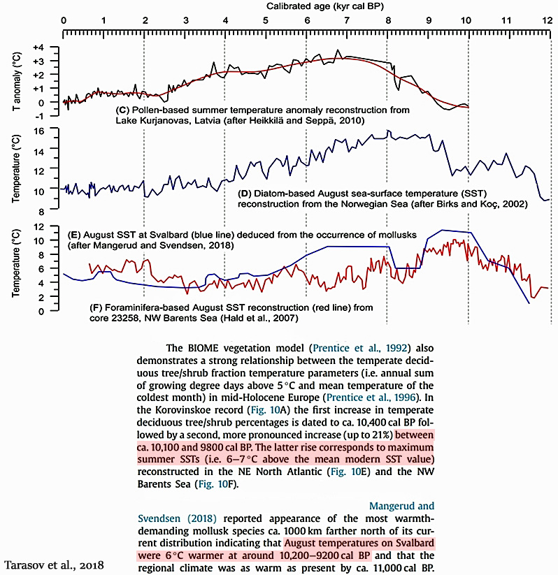
And of course, biological proxy data from all over the Arctic shows that for most of the last 10,000 years,
…. sea ice extent has been MUCH LOWER THAN CURRENT LEVELS
More KR fakery. These graphs have been doctored. PIP25 is not a unit of sea ice area. These are plots of a single biomarker in a single core. The claims that they represent sea ice extent were overwritten by KR. They were not made by the authors.
WRONG AGAIN, Nick
PIP25 is a very good PROXY for Arctic sea ice
DENIAL of science seems to be becoming the only thing left in your bag of old tricks.
Apart from rotating and making it more visual for morons like you by adding pointers to periods..
NO DATA HAS BEEN CHANGED, (unlike the AGW meme which is renowned for altering data)
Here is the original Stein graph, CLEARLY showing the words SEA ICE COVER.
You are either deliberately LYING or exposing your absolute mathematical incompetence in reading a basic graph..
“CLEARLY showing the words SEA ICE COVER”
with the qualitative terms “reduced”, “seasonal” and “perennial”, not numbers. How does that relate to Arctic sea ice extent?
In fact one thing KR erased from the graph was the title that it was for CORE ARA2B-1A. Not from “all over the Arctic”.
You poor muppet.
You will do ANYTHING to DENY the science of MUCH LESS Arctic sea ice through most of the last 10,000 years
Basic chart reading has become really difficult for you hasn’t it.
Reduced means.. reduced…..
Perennial means .. most of the year
What is SO COMPLICATED for you. !!
Even a 10 year old would understand that.
Has your mind really degenerated that much ?
I suggest you do some research and look at the works of Julianne Muller, where MANY c ores are used
In an attempt to educate Nick
Generally speaking, the PIP25 index correlates to sea ice extent as follows:
Actually, If you bothered finding the Stein paper, you would find he used 4 points from all over the Arctic, and they all have similar graphs showing much less sea ice for most of the last 10,000 years.
so, did you know that, and were DELIBERATELY LYING
Or were you just ignorant ?
The Sha graph also clears marks “Sea ice Concentration”
Do you need new reading glasses, Nick ???
It marks “concentration” in %. How does that relate to sea ice extent? In W Greenland?
In fact it is just an estimate at one drilling site.
And MANY other sites around the Arctic confirm this .. get over it.
DENIAL of science that shows the Arctic was MUCH WARMER and hence had MUCH LESS SEA ICE over most of the last 10,000 years, really doesn’t help your already empty reputation.
From Stein’s paper….
Reading comprehension is NOT something Nick seems to be able to do any more.
So sad to see a mind wasting away.
And Icelandic Sea ice charts show the 1970s extents being up with the EXTREME high levels of the LIA
https://notrickszone.com/2019/05/23/new-paper-arctic-sea-ice-was-far-less-extensive-than-today-during-the-ice-free-early-holocene/
sea-ice-was-far-less-extensive-than-today-during-the-ice-free-early-holocene
This is one of the most shamefully misleading articles I’ve ever read…
‘Study Shows Arctic Sea Ice Reached Lowest Point On Modern Record… In The 1940s, Not Today!’
Nowhere in the paper does it say that or conclude that. One graph, on volume, has been taken out of context and labelled with this misleading information.
and the actual information and conclusions – a summer ice free in 2050 for example -is utterly ignored.
Griff you may like to know that in 1984(year not book) a luxury cruise liner, ‘Linbad Explorer,’ carrying 98 “sophisticated international travellers” each of whom paid between 16,900 and 23,000 dollars completed the 4790 mile journey from St. John’s, Newfoundland to Point Barrow, Alaska in just 23 days.
You are late, but previewed 😀
https://wattsupwiththat.com/2021/01/24/study-shows-arctic-sea-ice-reached-lowest-point-on-modern-record-in-the-1940s-not-today/#comment-3168479
Griff
The data clearly show that up to the present Arctic sea ice variation in the last 2 centuries is normal and without particular trend.
The usual trick of starting from 1979 is the mother of all cherry-picks.
As so often, the story is “so far it looks normal but out computer models predict disaster any day now. Any day…”
Keep the faith bro!
You have the data-link, you have the script-link, your turn now to convince us, Whatsaboutthat ? 😀
WRONG.. the graph stands as it is..
There is NO misleading information.
It is a straight-forward extraction of the graph.. as shown above.
It’s just that your tiny brain-washed mind cannot acknowledge what it tells us.
Another case of the griff and its DELIBERATE IGNORANCE.
So many places.. ALWAYS the same result
MUCH LESS Arctci sea ice during most of the Holocene.
, maybe summer open Arctic.. far less than the approx 4 Wadhams we seem to be stuck at as a minimum.
And another one
The Early Holocene was about 6-7°C warmer than today in the NW Barents Sea region.
Does anyone really think this means there wasn’t a heck of a lot LESS sea ice than now ???
The Holocene sure is turning sour for the alarmists.
Keep up the good work!
A reader’s letter in the Sunday Telegraph, page 23 on Tuesday October 1st 2013 from Captain Derek Blacker RN (retd), Director of Naval Oceanography and Meteorology 1982-84 noted the following:
“I was a meteorologist during the Seventies when glaciers in Europe and other continents in Europe had been growing for the previous ten years, and pack ice had been increasing during winters to cover almost all of the Denmark Strait between Iceland and Greenland. Scientists were then warning that the Earth could be entering another ice age.
The current deliberations of the Intergovernmental Panel on Climate Change (IPCC) have conveniently overlooked this. Before insisting that humans have been the main cause of global warming an explanation of this apparent anomaly should be promulgated.”
Having read this letter, I had a look at information supplied by the Icelandic Meteorological Office. During the first two decades of the twentieth century (and I quote): ‘heavy sea ice was quite common along the coasts of Iceland, but in the 1920s a drastic change occurred. Sea ice along the coasts of Iceland became an uncommon characteristic and almost a forgotten phenomenon around the middle of the century. An abrupt change occurred in the mid-1960s. Heavy sea ice distribution occurred almost each year following, but since 1980 widespread and long-lasting sea ice off Iceland took place (sic) at rather irregular intervals’.
Some of the important fishing areas around Iceland are located on the shallow banks off the coast of Greenland at about 63ºN. These banks can be ice-covered during most of the year, causing difficulties for the fishing vessel. Ice edges form ‘tongues’ which extend like giant hooks when viewed from a satellite, extending for many kilometres (over 100km for example) and curving back towards the main ice sheet. These ice tongues, which can change rapidly from one day to another, are particularly important for fishing vessels operating near the ice edge. In some cases the ice tongues can turn back towards the main ice pack and vessels near the ice edge can be trapped. Consequently trawlers need accurate ice edge maps updated every day.
Meanwhile, cloud forcing FAR EXCEEDS any possible CO2 forcing at much higher atmospheric CO2 concentration
CO2 does diddly-squat !!
https://notrickszone.com/2021/01/25/scientists-determine-co2-levels-must-triple-to-yield-a-tiny-0-5-w-m%c2%b2-forcing-at-the-ocean-surface/
Another one bites the dust.
Thanks.
Observe from the graph the low somewhat after the warm era of mid-30s and the high somewhat after the cool era that ended around 1980. (I understand that Arctic may respond later than the rest of the earth.)
So no surprise to sensible people, but a revelation to anyone who has believed alarmists.
In 1940-1942 the reinforced wooden boat St. Roch traversed the Northwest Passage: St. Roch (ship) – Wikipedia.
Granted, Roald Amundsen did that in a colder period early in the century.
Of interest regarding Canada’s wimpy attempts to show sovereignty over the Arctic on this side of the earth, is that the St. Roch patrolled the Arctic for years, notably during the 1930s. (Operated by the Royal Canadian Mounted Police.)
I saw no mention here of the Danish Aerial survey photos of 1938. This showed significant recession of glaciers