26 October 2020
by Pat Frank
This essay extends the previously published evaluation of CMIP5 climate models to the predictive and physical reliability of CMIP6 global average air temperature projections.
Before proceeding, a heartfelt thank-you to Anthony and Charles the Moderator for providing such an excellent forum for the open communication of ideas, and for publishing my work. Having a voice is so very important. Especially these days when so many work to silence it.
I’ve previously posted about the predictive reliability of climate models on Watts Up With That (WUWT), here, here, here, and here. Those preferring a video presentation of the work can find it here. Full transparency requires noting Dr. Patrick Brown’s (now Prof. Brown at San Jose State University) video critique posted here, which was rebutted in the comments section below that video starting here.
Those reading through those comments will see that Dr. Brown displays no evident training in physical error analysis. He made the same freshman-level mistakes common to climate modelers, which are discussed in some detail here and here.
In our debate Dr. Brown was very civil and polite. He came across as a nice guy, and well-meaning. But in leaving him with no way to evaluate the accuracy and quality of data, his teachers and mentors betrayed him.
Lack of training in the evaluation of data quality is apparently an educational lacuna of most, if not all, AGW consensus climate scientists. They find no meaning in the critically central distinction between precision and accuracy. There can be no possible progress in science at all, when workers are not trained to critically evaluate the quality of their own data.
The best overall description of climate model errors is still Willie Soon, et al., 2001 Modeling climatic effects of anthropogenic carbon dioxide emissions: unknowns and uncertainties. Pretty much all the described simulation errors and short-coming remain true today.
Jerry Browning recently published some rigorous mathematical physics that exposes at their source the simulation errors Willie et al., described. He showed that the incorrectly formulated physical theory in climate models produces discontinuous heating/cooling terms that induce an “orders of magnitude” reduction in simulation accuracy.
These discontinuities would cause climate simulations to rapidly diverge, except that climate modelers suppress them with a hyper-viscous (molasses) atmosphere. Jerry’s paper provides the way out. Nevertheless, discontinuities and molasses atmospheres remain features in the new improved CMIP6 models.
In the 2013 Fifth Assessment Report (5AR), the IPCC used CMIP5 models to predict the future of global air temperatures. The up-coming 6AR will employ the up-graded CMIP6 models to forecast the thermal future awaiting us, should we continue to use fossil fuels.
CMIP6 cloud error and detection limits: Figure 1 compares the CMIP6-simulated global average annual cloud fraction with the measured cloud fraction, and displays their difference, between 65 degrees north and south latitude. The average annual root-mean-squared (rms) cloud fraction error is ±7.0%.
This error calibrates the average accuracy of CMIP6 models versus a known cloud fraction observable. Average annual CMIP5 cloud fraction rms error over the same latitudinal range is ±9.6%, indicating a CMIP6 27% improvement. Nonetheless, CMIP6 models still make significant simulation errors in global cloud fraction.

Figure 1 lines: red, MODIS + ISCCP2 annual average measured cloud fraction; blue, CMIP6 simulation (9 model average); green, (measured minus CMIP6) annual average calibration error (latitudinal rms error = ±7.0%).
The analysis to follow is a straight-forward extension to CMIP6 models, of the previous propagation of error applied to the air temperature projections of CMIP5 climate models.
Errors in simulating global cloud fraction produce downstream errors in the long-wave cloud forcing (LWCF) of the simulated climate. LWCF is a source of thermal energy flux in the troposphere.
Tropospheric thermal energy flux is the determinant of tropospheric air temperature. Simulation errors in LWCF produce uncertainties in the thermal flux of the simulated troposphere. These in turn inject uncertainty into projected air temperatures.
For further discussion, see here — Figure 2 and the surrounding text. The propagation of error paper linked above also provides an extensive discussion of this point.
The global annual average long-wave top-of-the-atmosphere (TOA) LWCF rms calibration error of CMIP6 models is ±2.7 Wm⁻² (28 model average obtained from Figure 18 here).
I was able to check the validity of that number, because the same source also provided the average annual LWCF error for the 27 CMIP5 models evaluated by Lauer and Hamilton. The Lauer and Hamilton CMIP5 rms annual average LWCF error is ±4 Wm⁻². Independent re-determination gave ±3.9 Wm⁻²; the same within round-off error.
The small matter of resolution: In comparison with CMIP6 LWCF calibration error (±2.7 Wm⁻²), the annual average increase in CO2 forcing between 1979 and 2015, data available from the EPA, is 0.025 Wm⁻². The annual average increase in the sum of all the forcings for all major GHGs over 1979-2015 is 0.035 Wm⁻².
So, the annual average CMIP6 LWCF calibration error (±2.7 Wm⁻²) is ±108 times larger than the annual average increase in forcing from CO2 emissions alone, and ±77 times larger than the annual average increase in forcing from all GHG emissions.
That is, a lower limit of CMIP6 resolution is ±77 times larger than the perturbation to be detected. This is a bit of an improvement over CMIP5 models, which exhibited a lower limit resolution ±114 times too large.
Analytical rigor typically requires the instrumental detection limit (resolution) to be 10 times smaller than the expected measurement magnitude. So, to fully detect a signal from CO2 or GHG emissions, current climate models will have to improve their resolution by nearly 1000-fold.
Another way to put the case is that CMIP6 climate models cannot possibly detect the impact, if any, of CO2 emissions or of GHG emissions on the terrestrial climate or on global air temperature.
This fact is destined to be ignored in the consensus climatology community.
Emulation validity: Papalexiou et al., 2020 observed that, the “credibility of climate projections is typically defined by how accurately climate models represent the historical variability and trends.” Figure 2 shows how well the linear equation previously used to emulate CMIP5 air temperature projections, reproduces GISS Temp anomalies.

Figure 2 lines: blue, GISS Temp 1880-2019 Land plus SST air temperature anomalies; red, emulation using only the Meinshausen RCP forcings for CO2+N2O+CH4+volcanic eruptions.
The emulation passes through the middle of the trend, and is especially good in the post-1950 region where air temperatures are purportedly driven by greenhouse gas (GHG) emissions. The non-linear temperature drops due to volcanic aerosols are successfully reproduced at 1902 (Mt. Pelée), 1963 (Mt. Agung), 1982 (El Chichón), and 1991 (Mt. Pinatubo). We can proceed, having demonstrated credibility to the published standard.
CMIP6 World: The new CMIP6 projections have new scenarios, the Shared Socioeconomic Pathways (SSPs).
These scenarios combine the Representative Concentration Pathways (RCPs) of the 5AR, with “quantitative and qualitative elements, based on worlds with various levels of challenges to mitigation and adaptation [with] new scenario storylines [that include] quantifications of associated population and income development … for use by the climate change research community.“
Increasingly developed descriptions of those storylines are available here, here, and here.
Emulation of CMIP6 air temperature projections below follows the identical method detailed in the propagation of error paper linked above.
The analysis here focuses on projections made using the CMIP6 IMAGE 3.0 earth system model. IMAGE 3.0 was constructed to incorporate all the extended information provided in the new SSPs. The IMAGE 3.0 simulations were chosen merely as a matter of convenience. The paper published in 2020 by van Vuulen, et al conveniently included both the SSP forcings and the resulting air temperature projections in its Figure 11. The published data were converted to points using DigitizeIt, a tool that has served me well.
Here’s a short descriptive quote for IMAGE 3.0: “IMAGE is an integrated assessment model framework that simulates global and regional environmental consequences of changes in human activities. The model is a simulation model, i.e. changes in model variables are calculated on the basis of the information from the previous time-step.
“[IMAGE simulations are driven by] two main systems: 1) the human or socio-economic system that describes the long-term development of human activities relevant for sustainable development; and 2) the earth system that describes changes in natural systems, such as the carbon and hydrological cycle and climate. The two systems are linked through emissions, land-use, climate feedbacks and potential human policy responses. (my bold)”
On Error-ridden Iterations: The sentence bolded above describes the step-wise simulation of a climate, in which each prior simulated climate state in the iterative calculation provides the initial conditions for subsequent climate state simulation, up through to the final simulated state. Simulation as a stepwise iteration is standard.
When the physical theory used in the simulation is wrong or incomplete, each new iterative initial state transmits its error into the subsequent state. Each subsequent state is then additionally subject to further-induced error from the operation of the incorrect physical theory on the error-ridden initial state.
Critically, and as a consequence of the step-wise iteration, systematic errors in each intermediate climate state are propagated into each subsequent climate state. The uncertainties from systematic errors then propagate forward through the simulation as the root-sum-square (rss).
Pertinently here, Jerry Browning’s paper analytically and rigorously demonstrated that climate models deploy an incorrect physical theory. Figure 1 above shows that one of the consequences is error in simulated cloud fraction.
In a projection of future climate states, the simulation physical errors are unknown because future observables are unavailable for comparison.
However, rss propagation of known model calibration error through the iterated steps produces a reliability statistic, by which the simulation can be evaluated.
The above summarizes the method used to assess projection reliability in the propagation paper and here: first calibrate the model against known targets, then propagate the calibration error through the iterative steps of a projection as the root-sum-square uncertainty. Repeat this process through to the final step that describes the predicted final future state.
The final root-sum-square (rss) uncertainty indicates the physical reliability of the final result, given that the physically true error in a futures prediction is unknowable.
This method is standard in the physical sciences, when ascertaining the reliability of a calculated or predictive result.
Emulation and Uncertainty: One of the major demonstrations in the error propagation paper was that advanced climate models project air temperature merely as a linear extrapolation of GHG forcing.

Figure 3, panel a: points are the IMAGE 3.0 air temperature projection of, blue, scenario SSP1; and red, scenario SSP3. Full lines are the emulations of the IMAGE 3.0 projections: blue, SSP1 projection, and red, SSP3 projection, made using the linear emulation equation described in the published analysis of CMIP5 models. Panel b is as in panel a, but also showing the expanding 1 s root-sum-square uncertainty envelopes produced when ±2.7 Wm⁻² of annual average LWCF calibration error is propagated through the SSP projections.
In Figure 3a above, the points show the air temperature projections of the SSP1 and SSP3 storylines, produced using the IMAGE 3.0 climate model. The lines in Figure 3a show the emulations of the IMAGE 3.0 projections, made using the linear emulation equation fully described in the error propagation paper (also in a 2008 article in Skeptic Magazine). The emulations are 0.997 (SSP1) or 0.999 (SSP3) correlated with the IMAGE 3.0 projections.
Figure 3b shows what happens when ±2.7 Wm⁻² of annual average LWCF calibration error is propagated through the IMAGE 3.0 SSP1 and SSP3 global air temperature projections.
The uncertainty envelopes are so large that the two SSP scenarios are statistically indistinguishable. It would be impossible to choose either projection or, by extension, any SSP air temperature projection, as more representative of evolving air temperature because any possible change in physically real air temperature is submerged within all the projection uncertainty envelopes.
An Interlude –There be Dragons: I’m going to entertain an aside here to forestall a previous hotly, insistently, and repeatedly asserted misunderstanding. Those uncertainty envelopes in Figure 3b are not physically real air temperatures. Do not entertain that mistaken idea for a second. Drive it from your mind. Squash its stirrings without mercy.
Those uncertainty bars do not imply future climate states 15 C warmer or 10 C cooler. Uncertainty bars describe a width where ignorance reigns. Their message is that projected future air temperatures are somewhere inside the uncertainty width. But no one knows the location. CMIP6 models cannot say anything more definite than that.
Inside those uncertainty bars is Terra Incognita. There be dragons.
For those who insist the uncertainty bars imply actual real physical air temperatures, consider how that thought succeeds against the necessity that a physically real ±C uncertainty requires a simultaneity of hot-and-cold states.
Uncertainty bars are strictly axial. They stand plus and minus on each side of a single (one) data point. To suppose two simultaneous, equal in magnitude but oppositely polarized, physical temperatures standing on a single point of simulated climate is to embrace a physical impossibility.
The idea impossibly requires Earth to occupy hot-house and ice-house global climate states simultaneously. Please, for those few who entertained the idea, put it firmly behind you. Close your eyes to it. Never raise it again.
And Now Back to Our Feature Presentation: The following Table provides selected IMAGE 3.0 SSP1 and SSP3 scenario projection anomalies and their corresponding uncertainties.
Table: IMAGE 3.0 Projected Air Temperatures and Uncertainties for Selected Simulation Years
| Storyline | 1 Year (C) | 10 Years (C) | 50 Years (C) | 90 years (C) |
| SSP1 | 1.0±1.8 | 1.2±4.2 | 2.2±9.0 | 3.0±12.1 |
| SSP3 | 1.0±1.2 | 1.2±4.1 | 2.5±8.9 | 3.9±11.9 |
Not one of those projected temperatures is different from physically meaningless. Not one of them tells us anything physically real about possible future air temperatures.
Several conclusions follow.
First, CMIP6 models, like their antecedents, project air temperatures as a linear extrapolation of forcing.
Second, CMIP6 climate models, like their antecedents, make large scale simulation errors in cloud fraction.
Third, CMIP6 climate models, like their antecedents, produce LWCF errors enormously larger than the tiny annual increase in tropospheric forcing produced by GHG emissions.
Fourth, CMIP6 climate models, like their antecedents, produce uncertainties so large and so immediate that air temperatures cannot be reliably projected even one year out.
Fifth, CMIP6 climate models, like their antecedents, will have to show about 1000-fold improved resolution to reliably detect a CO2 signal.
Sixth, CMIP6 climate models, like their antecedents, produce physically meaningless air temperature projections.
Seventh, CMIP6 climate models, like their antecedents, have no predictive value.
As before, the unavoidable conclusion is that an anthropogenic air temperature signal cannot have been, nor presently can be, evidenced in climate observables.
I’ll finish with an observation made once previously: we now know for certain that all the frenzy about CO₂ and climate was for nothing.
All the anguished adults; all the despairing young people; all the grammar school children frightened to tears and recriminations by lessons about coming doom, and death, and destruction; all the social strife and dislocation. All of it was for nothing.
All the blaming, all the character assassinations, all the damaged careers, all the excess winter fuel-poverty deaths, all the men, women, and children continuing to live with indoor smoke, all the enormous sums diverted, all the blighted landscapes, all the chopped and burned birds and the disrupted bats, all the huge monies transferred from the middle class to rich subsidy-farmers:
All for nothing.
Finally, a page out of Willis Eschenbach’s book (Willis always gets to the core of the issue), — if you take issue with this work in the comments, please quote my actual words.
Here’s a table of CMIP5 models, from AR5:
https://sealevel.info/AR5_Table_9.5_p.818.html
(Source here, or as a pdf, or as a spreadsheet, or as an image.)
The ECS values baked in to those models vary from 2.1 to 4.7 °C per doubling of CO2. The TCR values baked in to those models vary from 1.1 to 2.6 °C / doubling.
Such an enormous spread of values for such a basic parameter proves they have no clue how the Earth’s climate really works. What’s more, that’s just within the IPCC community. It doesn’t even include sensitivity estimates from climate realists.
Minor correction:
The IPCC has moved the AR5 report files, so that “source” link no longer works:
http://www.ipcc.ch/pdf/assessment-report/ar5/wg1/WG1AR5_Chapter09_FINAL.pdf#page=78
The new (working) link is:
https://archive.ipcc.ch/pdf/assessment-report/ar5/wg1/WG1AR5_Chapter09_FINAL.pdf#page=78
Note, also, in the first two columns, the large range of values assumed in the CMIP5 models for the even more fundamental parameter of Radiative Forcing.
Is there also a link to AR4? I want to study how the projections have been changing from report to report.
The AR4 (2007) WG1 Report’s main web page is here:
https://www.ipcc.ch/report/ar4/wg1/
The Report, itself, is here:
https://www.ipcc.ch/site/assets/uploads/2018/05/ar4_wg1_full_report-1.pdf
You can find other Reports here:
https://www.ipcc.ch/reports/
Very good point, Dave. They all deploy the same physics. They all are tuned to reproduce the 20th century trend in air temperature.
And yet they all exhibit very different ECS’s and produce a wide range of projections for identical forcing scenarios. Somehow this doesn’t ring alarm bells among them.
Are you familiar with Jeffrey Kiehl’s 2007 paper, “Twentieth century climate model response and climate sensitivity?
He discusses exactly the point you raise, and diagnoses it to alternative tuning parameter sets with off-setting errors. So, the models get the targets right, but vary strongly in the projections.
Thanks for the link!
Yes, there are two fundamental problems with GCMs (climate models).
● One is that they’re modeling poorly understood systems. The widely varying assumptions in the GCMs about parameters like radiative forcing and climate sensitivity proves that the Earth’s climate systems are poorly understood.
● The other problem is that their predictions are for so far into the future that they cannot be properly tested.
Computer modeling is used for many different things, and it is often very useful. But the utility and skillfulness of computer models depends on two or three criteria, depending on how you count:
1(a). how well the processes which they model are understood,
1(b). how faithfully those processes are simulated in the computer code, and
2. whether the models’ predictions can be repeatedly tested so that the models can be refined.
The best case is modeling of well-understood systems, with models which are repeatedly verified by testing their predictions against reality. Those models are typically very trustworthy.
When such testing isn’t possible, a model can still be useful, if you have high confidence that the models’ programmers thoroughly understood the physical process(es), and faithfully simulated them. That might be the case when modeling reasonably simple and well-understood processes, like PGR. Such models pass criterion #1(a), and hopefully criterion #1(b).
If the processes being modeled are poorly understood, then creating a skillful model is even more challenging. But it still might be possible, with sustained effort, if successive versions of the model can be repeatedly tested and refined.
Weather forecasting models are an example. The processes they model are very complex and poorly understood, but the weather models are nevertheless improving, because their predictions are continuously being tested, allowing the models to be refined. They fail criterion #1, but at least they pass criterion #2.
Computer models of poorly-understood systems are unlikely to ever be fit-for-purpose, unless they can be repeatedly tested against reality and, corrected, over and over. Even then it is challenging.
But what about models which meet none of these criteria?
I’m talking about GCMs, of course. They try to simulate the combined effects of many poorly-understood processes, over time periods much too long to allow repeated testing and refinement.
Even though weather models’ predictions are constantly being tested against reality, and improved, weather forecasts are still often very wrong. But imagine how bad they would be if they could NOT be tested against reality. Imagine how bad they would be if their predictions were for so far into the future that testing was impossible.
Unfortunately, GCMs are exactly like that. They model processes which are as poorly understood as weather processes, but GCMs’ predictions are for so far into the future that they are simply untestable within the code’s lifetime. So trusting GCMs becomes an act of Faith, not science.
(Worst of all are so-called “semi-empirical models,” which aren’t actually models at all, because they don’t even bother trying to understand or simulate the physical processes. Don’t even get me started.)
The egregious error is the absence of any representation of the mechanical processes of conversion of kinetic energy to potential energy within rising air and the reverse in falling air.
It is that missing component of a real atmosphere that results in the defects in the climate models described above in that they need to resort to numerous distortions of reality to get a fit with past observations.
As per Willis’s thermostat concept (which was a concept recognised by many others in earlier times) it is variability in the rate of convective overturning within an atmosphere that provides the thermostat.
The work by myself and Philip Mulholland describes the processes involved.
For those reading this who aren’t familiar with the reference, here’s “Willis’s thermostat concept” that Stephen is referring to, along with some of the “others in earlier times” that he mentioned:
https://sealevel.info/feedbacks.html#tropicalsst
That reference includes links to work by Ramanathan & Collins (1991), Dick Lindzen (2001), and Willis Eschenbach (2015).
(Stephen, would you mind sharing a link to “the work by [your]self and Philip Mulholland,” please?)
That said, I’m not too worried about the GCMs’ (weather models’) [in]eptitude when modeling “quick processes,” like you are discussing, because inept modeling of quick processes equally affects weather models.
When a weather model simulates something for which the underlying processes are poorly understood, or are too difficult to model, the problem is not hopeless. It is reasonable to hope that the ongoing process of comparing weather predictions to reality, and tweaking the weather model accordingly, will minimize the effects of those inaccuracies on the weather model’s output (weather predictions).
That obviously cannot happen with climate models, because their predictions are for the distant future, so they cannot be tested. But there’s a trend in the climate modeling world to build “unified models,” which model both weather and climate, using as much common code as possible. Basically, it means that they repurpose modules from weather models in climate models, to leverage the weather models testability, so that the climate modelers can have some confidence that those modeled processes are also modeled reasonably well in a climate model.
It is a reasonable idea. Since weather models get continually tested and refined, even if they don’t model an underlying mechanism correctly, there can be hope that their simulations of that meteorological process gives results that aren’t far from the mark.
The problem is that that only works for quick processes. There are also many slow processes which must be modeled correctly, if GCMs are to have any hope of being skillful — and the weather models do not simulate those processes.
For example, in 1988 Hansen et al used NASA GISS’s GCM Model II (a predecessor of the current Model E2) to predict future climate change, under several scenarios. They considered the combined effects of five anthropogenic greenhouse gases: CO2, CFC11, CFC12, N2O, and CH4.
They made many grotesque errors, and their projections were wildly inaccurate. But the mistake which affected their results the most was that they did not anticipate the large but slow CO2 feedbacks, which remove CO2 from the atmosphere at an accelerating rate, as CO2 levels rise. Oops!
Unified modeling cannot solve such problems. Weather models only model quick processes. They do not model processes that operate over decades, so unifying weather and climate models cannot solve the problems with modeling those processes.
Weather models are also updated with new measurement data every 2 hours or so. That means the model simulations are corrected with up-dated data several times a day.
Weather models are pulled back to physical reality repeatedly. That’s why 1-day weather predictions are much more reliable than 7-day predictions.
Updated with new physical measurements is obviously impossible for climate models.
Apart from the problems you listed, Dave, GISS Model II couldn’t model clouds, either. It hadn’t the resolution to predict the effects of CO2. Neither does GISS Model E2.
“Subsidy-Farmers” is too kind. “Socioeconomic Strip Miners” would be more descriptive.
Thank-you Anthony and Charles for this great science forum and for publishing my work!
Re: CIMP6 average cloud cover.
Look at the state of Washington, US. Try telling the residents of the eastern half that on average their climate is generally cloudy overcast rainy and cool. If cloud cover models fail so spectacularly over such a relatively small percentage of the planet then there is no way a global calculation is anything but guesswork.
Rainfall in Canberra is a good example of how badly weather predictions are. Always days late and much less than originally predicted. If a continuously updated weather computer can’t get it right, how do you plan to correct predictions made up to a century in the future?
Regarding error bars think of an out of focus photograph. Think of a news photo where a face has been blurred so that it can’t be recognized.
That’s a good and very accessible illustration Steve.
It’s almost exactly the analogy used in my 2008 Skeptic magazine article on the same topic.
Claiming modern climate models can detect the impact of CO2 emissions is like having a distorting lens before one’s eyes and insisting that an indefinable blurry blob is really a house with a cat in the window.
Perhaps better described as an iterative photo session with a somewhat blurred lens, where each photograph becomes the source for its immediate successor. Each take becomes less and less recognizable.
Think of a cheap, unmaintained photocopier making a copy of an old yellowed article, and then making a copy of the copy, and a copy of that copy, and so on. So far they are up to copy 6, not counting models previous to IPCC. The picture just gets fuzzier and fuzzier.
Judith Curry makes a strong point that a temperature increase of 6°C is flat out impossible. link If the models are producing temperature increases greater than 6°C, they don’t reflect what the climate system is capable of doing. Even if it is just an error bar, entertaining even the possibility of 15°C should demand extraordinary proof, ie. not just that a model said so.
Error bars extending to 15°C should be prima facie evidence that the models are wrong. Period. The burden of proof should be on those who say otherwise.
I think what is confusing the modelers is that major temp. swings actually did occur in the past.
https://notrickszone.com/2020/10/15/new-study-east-antarctica-was-up-to-6c-warmer-than-today-during-the-medieval-warm-period/#comments
And then they equate uncertainty bands with such recorded swings and shout eureka.
Unfortunately for the modelers, unlike Archimedes, they equate lead with gold.
Bob –> These are not error bars. It is an interval where you simply can’t know what the real value is. The ‘real’ part, let’s say 3.0 deg, is simply the center of the interval. It doesn’t mean thatit is an actual output or calculated true value. It is a way of indicating the center of the interval. The width of the interval is +/- 12.1 deg.
Any value within that interval is no more likely to be the actual value than any other value. Again, it is an interval defining what you don’t know and can never know.
“Any value within that interval is no more likely to be the actual value than any other value. ”
Uh, no. You are embarrassing even fellow deniers here. These probability distributions are absoltely not equi – probable. They are most likely normal, since most natural distribtions and most combinations of them, approach this.
But even if these pdf’s WERE square, the combo’s of them would tend to go to normal. Un;less these measurements were correlated, which is not the case here.
Get thee to your community college. Audit Engineering Statistics 101. I know you will need some pre requ’s, but audit them first. Just few used books, some time, a little gas, a VERY little tuition expense. The scales will fall from your eyes…
big –> Perhaps it is you that need an basic course in metrology. You are making the same error that Dr. Frank discusses. These are not statistical derivations of errors. They are derivations of uncertainty. I’ll say it again, these are intervals where you don’t know what the true value is and can never know. That means any value is as probable as any other value because you have no way to judge what the correctness of any given value is.
You are stuck in a statistics hole and apparently are having a hard time finding your way out. Statistics can be used to evaluate error when they meet certain requirements. You can not reduce or eliminate uncertainty with statistics. BTW, where did you get the idea that an uncertainty interval is a normal probability distribution? You didn’t even research Root Sum Square did you? I suggest you get “”An Introduction to Error Analysis” by Dr. John R. Taylor to get a rudimentary education in metrology.
“BTW, where did you get the idea that an uncertainty interval is a normal probability distribution? ”
Where did you ey the idea that I ever said it was? I was discussing uncertainly analyses of temp instruments, and their companion measurement processes ,which are CERTAINLY not uniformly distributed. Oh, and the known tendency of multiple such measurements to aggregate normally.
How do YOU think such measurement process error are distributed?
boB, “Where did you ey the idea that I ever said it was?”
You wrote probability distributions” and “pdf,” and wrote that they “are most likely normal,” all in your October 27, 2020 at 8:55 am boB.
Guess what that means.
[Hint: it means you said they’re normal probability distributions, just as Jim Gorman pointed out.]
Jim, “ I suggest you get “”An Introduction to Error Analysis” by Dr. John R. Taylor to get a rudimentary education in metrology.”
Thanks very much for that recommendation, Jim. I looked at the Table of Contents online and immediately ordered a copy of the 2nd Edition. It looks dead-on relevant. I wish I’d had that book 15 years ago.
I learned all my error analysis in Analytical Chemistry and an upper division Instrumental Methods lab, and also some in my Physics labs.
They stood me in good stead, but I’ve never had a book to lay it all out like Taylor looks to do. Not even Bevington and Robinson has that extensive a treatment.
Analytical chemists, in particular, are a bit like engineers because large economic consequences can follow their analyses, and sometimes even life-and-death. So, they have to get it right, and in my experience are very attentive to error and detail.
Pat –> re getting Dr. Taylors book. You are welcome. It is a good treatise to read before digging into the GUM. Even the GUM is light on using large databases of measurements and determining uncertainty .
> But even if these pdf’s WERE square, the combo’s of them would tend to go to normal. Un;less these measurements were correlated, which is not the case here.
Woah. How did you conclude these cumulative scenarios are comprised of independent variables that are both equi-probale and with no internal bias? I’m embarrassed you recommend Eng Stats for others before attending one yourself.
The point is that an uncertainty interval IS NOT a distribution of values that can be analyzed statistically. I know many folks have been raised on evaluating errors and sampled data using statistical tools. That drives many of them into a hole they simply can not climb out of.
An uncertainty interval is not made up of data points in a distribution that can be sampled to use the Central Limit Theory to derive a normal distribution and determine a mean and standard deviation. This is EXACTLY what Dr. Frank was attempting to explain that too many climate scientists DON’T understand.
“An uncertainty interval is not made up of data points in a distribution that can be sampled to use the Central Limit Theory to derive a normal distribution and determine a mean and standard deviation.”
A stnadard error of a trand can be computed exactly this way. With, or without error bands for the individual data points”
“This is EXACTLY what Dr. Frank was attempting to explain that too many climate scientists DON’T understand.”
You give not just climate scientists, but all scientists, too much credit. Pat’s irrelevant error propagation technique is so useless for AGW evaluation that NONE of them have cited it. Hence the utter lack of interest in his earth shaking paper.
Pat, the world’s just not ready for you. Too bad, especially in light of the fact that oilfield denier $ would, by orders of magnitude more than the “grant” $ whined about here, be there for you if it was…
“Pat’s
irrelevant highly relevant error propagation technique is souselessdevastating for AGW evaluation that NONE of themhave cited it.would DARE to even acknowledge it. “boB, “Pat’s irrelevant error propagation technique is so useless for AGW evaluation that NONE of them have cited it.”
““It is difficult to get a man to understand something, when his salary depends on his not understanding it.” — Upton Sinclair.
Error propagation is never irrelevant to an iterative calculation, boB. Never. Not ever.
Darn html ! try again.
“Pat’s
irrelevanthighly relevant error propagation technique is souselessdevastating for AGW evaluation that NONE of themhave cited itwould DARE to even acknowledge it. “You obviously were raised on statistics and have no clue about physical, real world measurements and their treatment. Now you jump to trends and how to evaluate a standard error. Standard Error is usually associated with a sample mean. Why do you think a sample procedure is needed with a temperature database of a station. The data is all you have and all you are going to ever have, in other words it is the entire population. Sampling a finite population that you already know buys you nothing. Just compute the mean and variance of the population and be done with it.
Again, you are mired in a statistical hole and refuse to stop digging.
I recommend studying-up on the GUM.
You’ve got it exactly right, Jim.
And, as usual, boB has it wrong.
Systematic error violates the assumptions of probability statistics and the Central Limit Theorem. They cannot be used to wish away uncertainty bounds.
Check out 2006 Vasquez and Whiting in the reference list of my paper, especially “2 RANDOM AND SYSTEMATIC
UNCERTAINTY.”
“Systematic error violates the assumptions of probability statistics and the Central Limit Theorem. They cannot be used to wish away uncertainty bounds.”
Didn’t say they could. Just that error propagation from an indefensible initial value, without regard to any physical constraints, has no place in AGW discussion. That’s why if you applied your propagation to any hind cast you would find the actual temps getting more and more implausibly close to P50, the farther out you looked….
And you wonder why the 99+% of those Dr, Evil conspirators ignore you. The best I can do is to point you to one of those Simpson’s scenes where Homer says something so “interesting” that it results in 15 seconds of dead air, and then a subject change….
… how ’bout those Dodgers, huh?
Error propagation has its place in any discussion of iterative calculations, boB. AGW is no immune fairyland.
I addressed your objection long since, here. See Figure 1 and the attendant discussion.
Climate model hindcasts do collect large uncertainties because the physical theory is poorly known. Conformance of a model simulation with past observables arises either from tuning or arises from a fortunate but adventitious parameterization suite that has conveniently offsetting errors.
The wide uncertainty bars inform us all that the simulation does not arise from a valid physical theory, and therefore hasn’t any physical meaning.
Modelers hide the physically real uncertainties in their hindcasts by tuning their models.
” ignore you”
They have to, because Pat completely destroys their fantasy narrative.
Your child-like tantrums don’t change that fact.
At the core, BoB believes that science is whatever he says it is.
What you’re saying is that the model output can be any value within those bounds and no value outside those bounds. What constraint makes that possible?
What Jim Gorman is saying is that the true physical magnitude can be any value within those bounds, but no value outside them.
Model output can be anywhere at all, depending on assumptions and parameters.
Just as an addendum, physical reasoning tells us that any future global average air temperature will probably not exceed past natural variation, say (+/-)6 C at the extremes, relative to current temps.
The uncertainties in Figure 3b are so wide as to exceed any possible physical reality. That just tells us the projection has no physical meaning at all.
Fully agree.
Any temperature increase is impossible. The energy balance is controlled precisely such that cooling ocean surface below 271.3K is literally impossible; it is no loner water but insulating ice. Likewise warming it above 305K is literally impossible. The rejection of insolation as that temperature is approached that the surface begins to cool.
The only exception to the latter, the Persian Gulf, proves the point. It is the only sea surface that has a temperature above 305K and it is the only sea surface that does not have monsoon or cyclones form over it due to the local topography.
The reflective power of monsoonal and cyclonic cloud is 3 times the reduction in OLR radiating power due to the dense cloud. SWR reflection in these conditions trumps OLR reduction by a factor of 3.
Any temperature reading purporting to represent “global temperature” that shows a warming trend should be viewed as a flawed measurement system. That is easily proven by observing the zero trend in the tropical moored buoys:
https://www.pmel.noaa.gov/tao/drupal/disdel/
Even when the system is disturbed by such significant events as volcanoes, the thermostat quickly restores the energy balance. It does a reasonable job over the annual cycle despite the large difference in insolation sea surface on a yearly cycle.
“Having a voice is so very important. Especially these days when so many work to silence it.”
Once again, the one man Pat Frank pity party. I’m reminded of Jon Stewart on Dennis Kucinich’s habit, as a presidential candidate, of beginning every debate response with “When I am president”.
Jon:
“I just want to to grab him by both lapels, pull him in to my face and yell “DUDE!!!!””.
Only in this case:
DUDE!!! Your paper has ONE citation! And it was just a bone thrown from a fellow chem guy. Even in the deniersphere it’s been first technically outed, and then ignored, as an embarrassment. Your FATALLY FLAWED, unitarily incorrect paper has NO relevance to AGW, IN ANY WAY.
Why am I not surprised to find that a progressive is upset when someone complains about the current cancel culture that he supports?
Why am I not surprised to find that a progressive is incapable of actually critiquing the science and instead attacks the author?
Yeah, another watermelon.
DUDE!!! Your paper has ONE citation!
Einstein’s paper
https://www.fourmilab.ch/etexts/einstein/specrel/specrel.pdf
Didn’t have any citations either.
“Einstein’s paper
Didn’t have any citations either.”
I think he wrote more than one. And most of them are not only widely cited, but are generally understood, world wide And I don’t think any of them would, if true, have invalidated nearly every forecasting technique, in every scientific and discipline we now use.
But more to the point, you are comparing ******* EINSTEIN to PAT FRANK???? Far *****’ out.
But I’ll throw you a bone. Pat and Al would both get about the same response if they linked their video’s to their eHarmony’s…
As usual, bugoilboob can’t be bothered with actually responding to the refutation of his previous point.
“but are generally understood”
That is the problem..
“Climate scientists™”, in toto” DO NOT UNDERSTAND the actual mathematics of error propagation.
BoB
DUDE….it’s an essay, and a good one, clearly pointing out the cumulative errors issue….
There are lot’s and lot’s of people that do not understand or appreciate cumulative errors.
They are essentially the same people that think it is reasonable to design in safety factor, multiply by another safety factor, and then add in freeboard. Safety factor, on top of safety factor, on top of safety factor; when you try to explain it to them they are oblivious (typically ignorant or stupid), don’t care/willfully ignorant (generally gov’t employees/democrats), or they rationalize it as “reasonable” (higher education/professional society/rule writers/politicians/selfish aholes).
None of the above being mutually exclusive. Wrt to Oily Bob, the list is likely mutually inclusive.
Combine Happer and van Wijngaarden’s findings on greenhouse saturation with this work by Pat Frank and the message in Ed Berry’s new book “Climate Miracle” and you can understand why no correlation can be found in properly detrended time series of CO2 changes and temperature changes. Now these are accompanied by hundreds of other data analysis papers that find no human signal in the global or regional temperature. The central focus of the consensus scientists should be to refute these rather than produce mounds of papers that ignore them in an attempt to convince the world of their correctness by having their stack out weigh this stack. One correct analysis that falsifies the others does just that unless it can be shown to be in error.
bigoilbob posted: “DUDE!!! Your paper has ONE citation!”
So, bigoilbob, please provide the specific reference that gives the number of citations required for a science-based article or paper, peer-reviewed or not.
If you cannot at least do that, I need not bother to ask you to provide your feedback as to where, specifically and upon what detailed argument(s), you conclude Mr. Frank’s article above is fatally flawed and incorrect.
DUDE!!! . . . just do it!!!
“So, bigoilbob, please provide the specific reference that gives the number of citations required for a science-based article or paper, peer-reviewed or not.”
For peer reviewed papers:
1. Bring up the paper.
2. Click on “article impact”.
For subterranean papers, no idea….
Typical, bugoilboob can’t actually refute the paper, so it invents a reason why it doesn’t need to even look at the paper.
“Typical, bugoilboob can’t actually refute the paper, so it invents a reason why it doesn’t need to even look at the paper.”
Again? It’s been done. Over and over. For years now. I don’t doubt that Pat et. al, in this fora will still carry on. But I am pleased to see how it has failed in the arena of actual scientific review, even amongst the “skeptics”. Actually, PARTICULARLY, among the “skeptics” who are especially embarrassed…
bigoilbob posted: “I am pleased to see how it has failed in the arena of actual scientific review, even amongst the ‘skeptics’.”
The first sentence of Pat Frank’s article above states “This essay extends the previously published evaluation of CMIP5 climate models . . .”
Therefore, it is impossible that the above essay has been subjected to “actual scientific review” allowing any judgement. It was, after all, just published today on the WUWT website.
Of course, certain individuals posting on WUWT have no problem whatsoever with engaging their mouth (and typing fingers) before engaging their brain.
boB< "Again? It’s been [refuted]. Over and over. For years now.”
It’s not been refuted once, boB (one is all it takes, after all). Et’s see you establish differently.
My 2008 Skeptic paper, transmitting the same method and message, hasn’t been refuted either.
“Again? It’s been done”
NO, it hasn’t.. only arguments have been like yours.. “arguments from IGNORANCE”.
bigoilbob, your response doesn’t even merit a “nice try”.
I specifically asked you for a source giving the number of citations REQUIRED for a scientific paper, and you respond with feedback about “impact” of a given paper . . . not even the impact of the number of citations provided in such a paper.
Care to try again . . . or just admit failure/inability to understand a simple request?
Like most trolls, the only mental skills that BoB has mastered are evasion and projection.
big –> Your ad hominem is ridiculous. Your argument consists of an argumentative fallacy of Appeal to Authority. If you want to prove something, do what none of those you described as showing this to be “technically outed” has done, show the math is wrong. The only argument I have seen is that the +/- 4 W/m^2 is wrong, not the math and not the procedure. Funny how it is now +/- 2.7!
You want to show your smarts, tell everyone how you calculate the uncertainty in a machining process with 10 iterative steps (one must be completed before the next one). I bet you’ll find RSS (root sum square) is the method used.
Another meritless rant, boB. Good job.
Your awkwardly phrased “unitarily incorrect,” just blindly repeats Nick Stokes’ failed argument from willful ignorance.
And speaking of arguments, yours always seem to be arguments from preferred authority. You’re apparently a trained geologist, Bob. Can’t you do a little independent thinking and compose critical arguments of your own?
“You’re apparently a trained geologist, Bob. ”
You give me too much credit. Adult lifelong, private sector, petroleum engineer, US and international. No tenure, no senioritized sinecure, no reliance on the guv for my funding Ooh, sorry….
I’m scientific staff, boB. No tenure, no senioritized sinecure, no reliance on the guv for my funding Ooh, sorry…..
He certainly seems to have touched a nerve with you! Good!
What has he said which is false?
Good grief, bigoilbob, that’s a scathing statement. So what is wrong with Pat’s analysis? In an iterative simulation (“model”) where the result of every iteration becomes the initial state for the next iteration, how is it possible to NOT accumulate errors until the results bear no relation at all to any possible configuration of reality? Eh?
Unless the errors are vanishingly small for every iteration? Which they are not, are they? Not when whole weather systems can come and go within a single cell of the coarse grid they use to subdivide the atmosphere.
Pat puts his focus on the effect of propagating errors through multiple iterations. That is the field he is a specialist in. It is only one of the failings of climate science as it is practiced today. In fact the whole climate science edifice is nothing but errors piled on errors based on plausible-sounding but unverified assumptions. That is what “science” looks like when the conclusions have been determined in advance of the “study”.
Pat asserts (correctly) that CMIP6 models, just like their five predecessors, have no value. He is wrong. They have no value as scientific predictions of future climate states, true, but their real value is that in guiding gullible politicians and their media enablers towards so-called “green” policies that favour de-industrialization and redistribution of wealth.
Is anyone really surprised that CMIP6 predicts more warming than CMIP5? Does anyone doubt that CMIPs 7, 8, 9 etc. will predict progressively more warming? Of course not! It’s Climate Science, the industry that manufactures fear, where it’s always “Worse Than We Thought”. Where it needs to be always “Worse Than We Thought” because people get tired of predictions of doom that are always off in the future.
bigoilbob – why are you shouting? Got a point to make, like how Pat Frank is wrong, show us your proof.
Otherwise you are just shouty, armwavy ignorable.
The entire low frequency response of climate models is simply driven by the prior model inputs (the forcings). Climate models are just random noise generators. That’s why you can only see the signal after averaging loads of models. Subtract the model average form the individual models and what is revealed is uncorrelated noise. Try it for yourself.
This is how a climate model works:
climate model output = input forcing prior model + noise
So sad that the big oily blob doesn’t comprehend basic maths and physics.
All we get is just another empty rant from a bitter and twisted AGW apologist.
Show us where Pat is wrong…..
….. or stop the very comical tantrums, big oily blob .
The guy has annihilated you and all you have left is ad hominem attacks. It’s just ridiculous.
The idea that an extremely complex, poorly understood, system like Earth’s climate would have models that are replete with theory error should be common sense. Billions of dollars of people overfitting the data to be right for the wrong reason and being wrong in the future for a ever-growing pile of excuses.
Don’t embarrass WUWT. This has been covered. It’s a moderating system. You don’t add the errors. They more or less cancel. I am speaking to everyone going against bigoilbob. The climate system is complex but it keeps cancelling things out. If there’s a warm spot somewhere, it doesn’t stay warm and add the same warmth to the spot next to it. Everything that’s different tends back to the average. You’re arguing for a sleight of hand. Each Summer the NH warms. The each Winter it cools. Who in their right mind would just keep adding the Summer warming? Not everything gets to go in one direction.
“Not everything gets to go in one direction.”
You are obviously n o “up with” climate science™.
Haven’t you seen the “adjusted” graphs of temperature for sites in GISS.
Everything HAS TO go the same direction, after they have finished.
You’ve evidently misunderstood the meaning of error propagation, Ragnaar.
“An uncertainty in the base state may be important, but if you’re more interested in a how a system changes in response to some external influence, then it may not be that important. Your final state may not be accurate, but you may still be able to reasonably estimate the change between the initial and the final state. The uncertainty in cloud forcing is really a base state error, not an uncertainty between each step (i.e., you don’t expect the cloud forcing in a climate model to be uncertain by +-4 W/m^2 at each step).” – ATTP
In just one step, +-4 W/m^2. What happens next? It’s warmer or cooler by a lot. Does it tail into runaway warming or cooling? No. You can say we don’t if it’s plus or minus. I’ll say it’s both depending on how I feel. The pluses and the minuses average back to zero. We have: +-4 W/m^2. Why? Because it’s useful. How do we know it’s useful. We use it.
If we got the results in figure 3b you could be right. We don’t usually because the base state errors are controlled. A CMIP is stable. It just goes to a higher stable place. It’s just a question of how high. Antarctica’s total collapse would have little to do with error propagation. They call it unstable but I call it stable. It’s a lot of ice and pretty cold. 500 years is stable to me.
There’s a lot wrong with the CMIPs. But the climate is stable as are the CMIPs.
You can’t keep taking one side of a bell curve distribution. The +-4 W/m^2 applies to the whole thing, not the steps. A bell curve distribution itself is not one iteration. It’s a lot of them. It would be like taking Tyrus and cloning him. And then saying this is what happens. The CMIPs spit out all Tryuses. But they don’t.
Ragnaar, ±4 W/m^2 is not an energy. It does not represent a perturbation on the model. It does not affect the simulation.
And, look, you’re so eager to find a mistake that you’ve blinded yourself to the realization that, taking the meaning of ±4 W/m^2 as you intend, then:
±4 W/m^2 = +4W/m^2 – 4 W/m^2 = 0.
No net perturbation at all. Where does your warming or cooling come from?
From where does your supposed model instability come when the net perturbation is zero?
Don’t feel too badly, though, because research level climate scientists, including ATTP, have made the same blinded mistake.
A ±4 W/m^2 calibration error statistic has nothing to do with runaway or collapsing anything. It does not affect a simulation, a projection, or anything a model does.
Next: ATTP is wrong in his appraisal. The ±4 W/m^2 is not a base state error. The ±4 W/m^2 is a rms model calibration error coming from comparison of 20 years of hindcast simulation with 20 years of observation.
They averaged over 27 CMIP5 models, for 540 total simulation years.
All those models were spun up in their base year. Then they were used to simulate the 20th century. Then their simulations were compared with observations at every grid-point. Observed minus simulated = error. Calculate the global rms error.
The ±4 W/m^2 is the annual average rms uncertainty in long wave cloud forcing in every single year of those 20 years of simulated climate.
Twenty years of hindcast simulation does not represent a base state.
The error envelope in Figure 3b does not indicate model output — another freshman mistake ubiquitous among climate modelers.
Look at 3b carefully, Ragnaar. Do you see those lines right in the center? Those are the model outputs.
See the envelopes? Those are the uncertainties — not the errors, not the projection variation about the mean, not any representation of any model output.
Those envelopes are what we can believe about those projections. Those envelopes represent the physical information content.
They tell us that there is no physical meaning at all in those projected temperatures.
Pat Frank:
±4 W/m^2
Say you double CO2. And say you get: ±4 W/m^2. It could be simply turning the furnace on. How much does the furnace warm the house? X + – 4Y. Are you going to get radically diverging temperatures in the house? No. If you calculate it every 10 minutes, no. If you calculate it twice a day. No. Because the house plus the furnace running gives a stable temperature during the heating season. You don’t know if heating the house gives you X, 1.4X, or 0.6X. But you do know it does not go to infinity. And you know once the furnace reaches a stable temparature it stays there, even if it’s too hot or too cold. CO2 warming by more or less does that. It doesn’t run to infinity. The climate is stable and it has a thermostat. The models are stable and have a control knob. Just because something isn’t known well enough, doesn’t mean the system returns wild values like your plot does. If you are making tools within a tolerance, it works fine. You don’t even do a calculation like you want to do. But if you did it, you could compare that to what actually happened with the tools. All the CMIPs did is get the impact of CO2 too high. That’s it. End of story. From here on out, it’s just a boring thing with them saying wait until next year when it will be warmer. Let’s say I am still off base. Use an analogy. Notice how Willis tells a story. Do that. This is not rocket science. You ought to be able to communicate to someone. Tell a story about tools being made not perfectly. What ever it is your saying applies to more than CMIPs. Because good ideas repeat themselves and are found all over the place. Bad ideas, not so much. Ideas that don’t spread lose the evolutionary race.
Ragnaar, the first sentence in the post above yours tells you that the ±4 W/m^2 is not an energy. It is a calibration error statistic.
It can’t heat a house. A million of them can’t heat a house
The ±4 W/m^2 has no physical existence.
You’re arguing nonsense. Your argument is nonsense. You have no idea what you’re talking about.
You need to find a book about physical error analysis and read about the meaning of calibration, resolution, iterative calculations, and propagation of error.
You clearly know nothing of any of that.
Maybe you can go to a library and consult a copy of John Taylor’s Introduction to Error Analysis: The Study of Uncertainties in Physical Measurements . Jim Gorman recommended that book and Jim knows what he’s talking about.
You need to do some silent study.
Use an analogy. Notice how Willis tells a story. Do that. This is not rocket science.
I got you beat on telling stories. You’re point is not getting across. All your supporters should tell a story that proves your point. Or the situation is, No story can be constructed about your point.
Story, schmory, Ragnaar. You still don’t know what you’re talking about.
Ragnaar , you’re not adding warming each year, nor are you adding cooling. You’re accumulating errors, which increases your cone of ignorance. Moreover, climate models have offsetting errors which deliberately constrain the trend. No climatologist would publish a model that exploded to infinity or collapsed to absolute zero, because they would be laughed out of the door. They release model runs that have constrained solutions, only for completely nonsensical reasons because the physical reality of the world is not represented. Any time a model spits out nonsense, the Deus ex Machina steps in and rewrites the laws of the physical world with some parameterization or something else.
Pat, thank you for updating this important work. I think the CMIP6 projections are worse than we think – not only are they insignificant relative to model error, the models themselves, based on your Figure 2, would appear to have been tuned / calibrated to agree with the GISS version of global temperature anamolies.
“to agree with the GISS version of global temperature anamolies.”
Which means that they have FABRICATED WARMING baked into them.
To get a realistic result, they would have to “de-adjust” the fabrications and mal-adjustments in GISS….
… but then their scare story would disappear.
“”Oh, what a tangled web we weave, when first we practice to deceive!””
Or a huge Catch22 situation. 🙂
““to agree with the GISS version of global temperature anamolies.””
The climate modelers ought to try to get their models to agree with the United States temperatures, since the U.S. temperature profile represents the global temperature profile.
GISS is science fiction. The computer models are agreeing with science fiction, which makes the computer models science fiction, too.
Thanks, Frank.
Figure 2 shows that the climate model linear emulation equation (eqn. 1 in my paper), can also emulate the historical air temperature record just using the standard Meinhausen forcings.
That Figure is a bit of a deliberate irony, actually, because it shows the linear equation passes a supposedly rigorous standard that climate models must pass to show their validity.
“with a hyper-viscous (molasses) atmosphere”
That would explain why the models show no increased convection when the atmosphere warms and gets more humid.
Which is yet another MAJOR error. !
Accuracy vs precision.
https://blog.minitab.com/blog/real-world-quality-improvement/accuracy-vs-precision-whats-the-difference
I was thinking about how alarmists like to claim that more measurements makes their average more accurate.
Using the same instrument to measure the same thing repeatedly, might improve accuracy, but it does nothing for precision. That is, repeated measurements will reduce sampling error, but any errors introduced by the tool itself will remain.
Using multiple instruments to measure the same thing will make it more accurate but does nothing for precision.
Using multiple instruments to measure multiple things (as climate science does) does nothing for either accuracy or precision.
“but any errors introduced by the tool itself will remain.”
This is what gun sight adjustments are for. And the adjustments any CAM operator learns to use in his/her apprenticeship. And the KNOWN “precision” biases for every temp measuring device used in the last 2 centuries….
bugOilBoob really has faith in the ability of his masters to re-write the past accurately.
First off, as any shooter knows, you have to constantly re-site your rifle if you want it to stay accurate.
Who’s recalibrating the temperature sensors for the last 2 centuries?
Secondly, knowing the average accuracy of a class of probe tells us little to nothing about the accuracy of a particular unit. Especially after it has been in the field for several years.
“First off, as any shooter knows, you have to constantly re-site your rifle if you want it to stay accurate.
Who’s recalibrating the temperature sensors for the last 2 centuries?”
How’z about the people who used them, maintained them, and kept assiduous use records on them. Do you think that measurement bias is revealed truth for only he last generation?
“Secondly, knowing the average accuracy of a class of probe tells us little to nothing about the accuracy of a particular unit.”
So, some might swing one way, or not, for awhile, and then that swing will be corrected. And? How can this be source of significant measurement bias, considering that the evaluations under discussion involve tens of thousands of measurements, taken over hundreds of months, involving time based changes orders of magnitude higher.
FFS, folks, whether you’re whining about normal measurement error or transient, correctable (and mostly corrected) systemic measurement biases, they ALL go away, as a practical matter, when considering regional/world wide changes over climactic physically/statistically significant time periods.
You claim that they people who used them were re-calibrating.
Where’s your evidence that this was occuring.
I love the way you just assume that all errors must cancel out. Once again you demonstrate that you know nothing about instrumentation.
Finally, bugoilboob wants us to believe, without evidence, that the temperature measurements over the last 100 years are close enough to perfect that error bars aren’t needed.
“You claim that they people who used them were re-calibrating.
Where’s your evidence that this was occuring.”
Because they knew they had to. Because the instruments were regularly reapired/replaced.
“I love the way you just assume that all errors must cancel out. ”
Since they go either way, they minimize. They don’t “cancel out” and that’s why I didn’t say they did. Stat 101, DO YOU SPEAK IT?
“Finally, bugoilboob wants us to believe, without evidence, that the temperature measurements over the last 100 years are close enough to perfect that error bars aren’t needed.”
Error bars ARE needed. That’s why they are provided in either the root data bases or in the availabe info on the devices and measurement processes. And that’s how we know that they mean practically nothing at all to the error in the evaluated trends
“You claim that they people who used them were re-calibrating.
Where’s your evidence that this was occuring.”
That they knew what they were doing. That the instruments were repaired and replaced as needed.
“I love the way you just assume that all errors must cancel out. ”
Why do you “love” what I didn’t say? They DO minimize, per stat 101 – DO YOU SPEAK IT?
“Finally, bugoilboob wants us to believe, without evidence, that the temperature measurements over the last 100 years are close enough to perfect that error bars aren’t needed.”
Again, why would I “want you to believe” something that I don’t? The “error bars” are (1) available, along with errors introduced from the rest of the measurement/recording processes, and (2) show us that, for our purposes, they matter not at all.
“FFS, folks, whether you’re whining about normal measurement error or transient, correctable (and mostly corrected) systemic measurement biases, they ALL go away, as a practical matter, when considering regional/world wide changes over climactic physically/statistically significant time periods.”
FFS Bob, apparently they don’t ALL go away given the error in cloud cover / forcing relative to the degree of projected warming. There’s a difference between strapping pipe with an accurate tape (small random errors that offset to some degree) vs an inaccurate tape (systematic errors that do not offset). The former allows you to make reasonable inferences about depth; the latter gets you run off the rig.
big –> “FFS, folks, whether you’re whining about normal measurement error or transient, correctable (and mostly corrected) systemic measurement biases, they ALL go away, as a practical matter, when considering regional/world wide changes over climactic physically/statistically significant time periods.”
You still refuse to acknowledge what uncertainty is. Every “regional/world wide changes” begins with individual measurements. Those measurements have uncertainties that should be propagated throughout the series. You are trying to hint that traditional statistical treatments of a population will remove uncertainty. IT WON’T! Calculating an error of the mean that is 6 decimal places long simply doesn’t change uncertainty at all.
” So, some might swing one way, or not, for awhile, and then that swing will be corrected. And? How can this be source of significant measurement bias, considering that the evaluations under discussion involve tens of thousands of measurements, taken over hundreds of months, involving time based changes orders of magnitude higher.”
How does this explain making constant “corrections” to temperature measurements 50 years old?
“So, some might swing one way, or not, for awhile, and then that swing will be corrected. And? How can this be source of significant measurement bias, considering that the evaluations under discussion involve tens of thousands of measurements, taken over hundreds of months, involving time based changes orders of magnitude higher.”
We are not talking about bias but demonstrated uncertainty. If all the thermometers were properly calibrated and read there is still systemic error. In an electronic distance meter it is give as a length and a PPM (2mm± 3PPM) uncertainty. In a rifle it is expressed as Minuets of Accuracy (MOA). That uncertainty propagates with each iteration that depends on the results of the previous one. There is a mathematical process used to compute the reliability of processes with error or uncertainty propagation. That is what Dr. Frank has used to calculate the reliability of the models.
B.O.B.
You said, “Since they go either way, they minimize.” That is true of random errors. However, systematic errors that are the result of things like component aging, corrosion, dirt accumulating, etc., are more likely to move in only one direction, depending on the dominant factor affecting the accuracy.
I’m reminded of the line from Hamlet, “The lady doth protest too much, methinks.” You seem to be going to extraordinary efforts to discredit a claim you disagree with, without bringing any real new evidence to the party, or even demonstrating error in Pat’s logic. Be careful, the unwary might mistake you for an astroloclimatologist instead of the engineer you claim to be. Your ad hominems are certainly less than convincing!
“That is true of random errors. However, systematic errors that are the result of things like component aging, corrosion, dirt accumulating, etc., are more likely to move in only one direction, depending on the dominant factor affecting the accuracy.”
So, these trends weren’t recognized, by technicians/measurement experts? For some perspective, most of the data they evaluated was post non astronomical speed of light calculation.
So, this is still true when technicians are evaluating thousands of these instruments at the same time, all of which are being randomly repaired, readjusted, replaced, over many decades?
Yes, gun sights do go out of adjustment. No, not relevant to the evaluation of the many decades (i.e. hundreds) of data sets, each with populations in the many hundreds/thousands, using instruments/methodology well understood and managed, now under discussion.
Try harder, Clyde….
” or even demonstrating error in Pat’s logic.”
Been done, many times before. In this forum. With your contribution, but NO tech refutation, from you.
It’s not really about the truth any more, is it, Clyde….
big,
1. error is not uncertainty. Learn it, love it, live it.
2. What happens when someone who is 5′ tall reads a mercury thermometer one day a 100 years ago and then someone 6′ tall reads it the day following? It doesn’t matter how accurately the thermometer is calibrated, parallax alone will generate an uncertainty as to what the true value of the measurements. Even the newest Argo floats are estimated to have uncertainty somewhere between +/- 0.5 to +/- 1.0 degrees because of various conditions associated with the float itself (e.g. salinity of the sample, dirt in the water flow tubes, etc.) It doesn’t matter how closely the float was calibrated, some things just can’t be controlled during the measurement – leading to an uncertainty in the measurement.
Once again, when asked for specifics, the only thing bugoilboob does is just make more unsourced claims.
big
You are right, gun sights are not relevant. That is why I didn’t mention them. Try harder.
boB, “Been done, many times before. In this forum.”
No, it hasn’t. Not once. And you can’t provide an example. Not one.
“It’s not really about the truth any more”
big oily blob has done all he can to steer it away from the truth.
And utterly failed. !
The AGW farce never was about the truth anyway.
And buckshot resolution, accuracy, precision? The modelers couldn’t hit a barn door!
I agree bonbon.
And BoB talked about truth! Is that like the cataclysmic predictions that ‘climate scientists’ have been promising us for the last 50 years BoB? That truth?
That our major dams would dry up? That’s been a good one, been used many times over the decades. Hasn’t happened though so that can’t be true.
That it would not be possible to feed the global population due to crop failures on a massive scale? That truth? Oh I forgot, we are experiencing record crops year after year.
That low level islands would disappear with rising sea waters, and whole cities will disappear too? No, that hasn’t happened. I have heard that some are growing though, islands and cities.
How about the disappearing polar bears? Ah, the symbol of ‘climate change’. Is that the truth you’re talking about? Oh that’s right you aren’t allowed to hunt them any more and their numbers have increased significantly!
It must be the about the coral reefs, yes that must be the truth you’re talking about. A ‘climate scientist’ in Australia has declared the Great Barrier Reef half dead, all due to global warming. And he should know, he flew over it in an aeroplane. I do know that we have impressive cyclone events up that way, and the crown of thorn starfish get out of hand from time to time. Hungry little buggers. So ‘climate change’? No that’s a lie too, our friend Jennifer spent a week diving in the waters that were supposed to be the worst affected last January, she couldn’t find any signs of significant bleaching. She showed us the video too.
Unprecedented rising temperatures! That’s the ‘truth’ you’re talking about! Except that previous high temperatures have been wiped from history, and they bring up particular temperatures as ‘unprecedented’, and I know that I have personally experienced higher temperatures myself! They leave out and change so many figures that no intelligent person could ever trust them. And they don’t talk about the unprecedented ‘low’ temperatures.
All this truth BoB! And then they say “The science is settled”, “You can trust the science!” Why would I BoB? I can’t and I won’t, I’ve been lied to for too long. Why would anyone ‘choose’ to believe that the world is approaching crisis. Isn’t it preferable to think that just maybe ‘the science’ was wrong? If there was any integrity in ‘climate science’ at all, wouldn’t they be keen to look at the potential that they may have been wrong? Why is the end of world scenario preferable?
You are here playing the leftists political game BoB, attack the man first and foremost, then attack the institution. You are seeking to bring down the integrity of the writer here BoB, same method as the ‘climate scientists’. Not willing to look at having a real conversation, so afraid of being proven wrong.
And as for ‘computer games’, even the very best of them are only as good as the information they are fed. Creative accounting is where a good accountant can come up with the ‘requested’ figures. I’m sure it’s works the same way with science.
The truth is BoB, they need to keep the lie alive. The whole climate scam is making a handful of people very rich by way of ‘the cure’, all forms of renewables. Do you have skin in the game BoB? How much do you have invested in the renewables industry?
And as for ‘computer games’, even the very best of them are only as good as the information they are fed. Creative accounting is where a good accountant can come up with the ‘requested’ figures. I’m sure it’s works the same way with science.
big –> Gun sight adjustments don’t eliminate errors. Otherwise you could shoot every bullet through the same hole every time. CAM operators also learn what uncertainty, otherwise known as tolerances, actually means.
As to precision biases, that is not a good term. Biases don’t affect precision, uncertainty does. Look up repeatability in measurements. You don’t calibrate precision, you calibrate accuracy. You want better precision, get a better instrument.
As far as temps in the last two centuries, it is the recorded number that is important. An integer recording of 75 deg has a minimum uncertainty of +/- 0.5 deg, like it or not. You and nobody else can go back in time or place to monitor how the temp was actually taken. You must use what was written down.
“big –> Gun sight adjustments don’t eliminate errors. Otherwise you could shoot every bullet through the same hole every time. ”
No, there would still be scatter. But, to the extent that you adjusted correctly, you would be shooting more shots closer.
Folks, this is why we have blogs and actual peer reviewed exchanges…..
big –> “But, to the extent that you adjusted correctly, you would be shooting more shots closer.”
Actually no. Their average may be closer to the true value, i.e., the bulls eye, but that is accuracy, not precision. Precision is the spread. You can calibrate all you want, but if your precision is a 4 degree (4 in at 100 yds) circle, all of the calibration you you can do will never change that. Been there, done that. Get a better instrument, i.e. rifle.
Well this is a silly claim, platinum RTDs were not in widespread use 200 years ago. And what exactly is a ‘KNOWN “precision” biases’?
“platinum RTDs were not in widespread use 200 years ago.”
And? The question is whether or not the meters/methods in use at the time, in combo with those we have used more recently, were fit for our current uses. Given that even the most pessimistic guesses on individual error bands and/or short term residual shifts of even the worst of them, are tiny and fleeting w.r.t. the trends we seek, they were QUITE good enough.
(+/-)2C versus 0.001C or even 0.01C? There is a bit of a disconnect here.
What is the standard deviation of any single global average temperature point?
Meteorology field stations are exposed to sunlight, either directly or by reflection.
When air flow is less than about 3 m/sec, even a well-sited thermometer shield heats and the air within the measurement volume is warmer than the outside air. The measured temperature is too high.
In the Winter, cold still air under a cloudless sky cools the thermometer shield below the air temperature. The measured temperature is too low.
These systematic errors are ubiquitous everywhere a meteorological station is located. Such systematic errors are not removed by averaging but have never been taken into account in any published global air temperature record.
The resultant uncertainty in global air temperature is about (+/-)0.5 C (900 kb pdf), which obviates the entire thermal trend since 1900 at the 95% confidence level.
I’ve had email conversations with some of the UKMet people. They refuse to acknowledge the existence of systematic measurement error, even though there is plenty of evidence in the published literature.
And everyone here has seen how BEST responds in the person of Steve Mosher. Hostile rejection.
I’ve finished further work on the record. Writing it up is ratcheting closer as time permits.
When everyone sees the analytical details and errors these people have overlooked in their facile carelessness, the play-science of these consensus incompetents will be fully on display.
Pat,
It isn’t just systematic errors. When you calculate an average to use in calculating anomalies and carry that average out to decimal places not warranted by the precision of the recorded temps you are misstating the precision. Subtracting a mean of 75.345 (that was calculated by using integer temps) from integer temps and keeping the decimal places violate every rule of significant digits I was ever taught.
I often quote this statement from Washington Univ. at St. Louis Chemistry Dept. “Significant Figures: The number of digits used to express a measured or calculated quantity.
By using significant figures, we can show how precise a number is. If we express a number beyond the place to which we have actually measured (and are therefore certain of), we compromise the integrity of what this number is representing. It is important after learning and understanding significant figures to use them properly throughout your scientific career.”
Ask yourself how climate scientists justify anomalies out to 3 decimal places when using integer temperatures.
I completely agree with you, Jim. They claim significant figures well past the measurement resolution.
I’ve had arguments with Nick Stokes about that. He doesn’t understand resolution at all. Every instrument is perfectly accurate and infinitely precise.
The LiG thermometers historically used had 1 C divisions (except when they had 2 C divisions; or ships’ thermometers were often 5 C divisions). But anyway, you’re anticipating this but it’s worth saying out loud, the standard field reading resolution is ±0.25 C.
That ±0.25 C is the minimum of uncertainty in every field reading. But UKMet, GISS, BEST and all the rest brush it aside. Resolution appears nowhere in any of their papers. I’ve never found that word in the published works. And I’ve looked.
Not only that, but when they take anomalies, they don’t calculate the quadratic sum of errors to properly qualify the difference.
They make lab mistakes that are weeded out of students in their first year. These people are a bunch of refractory incompetents, the lot of them.
Let me take this opportunity to thank you for your indefatigable efforts in illuminating the meaning of uncertainty and systematic error. It’s been a pleasure to see and read. Thanks Jim (and thank Tim for me too, please, if he’s related and not you).
Pat, We are related and look alike, a lot!
Climate models are like firing a wide-mouth blunderbuss firing bird-shot …… blindfolded.. 🙂
still wrong, not even wrong
Once again, steve can’t be bothered to refute anything. I guess he’s convinced that someone with his stellar credential in English can’t be wrong so must never be questioned.
My that’s a detailed basis for your pronouncement…..
He get’s to the same point as BoB, with fewer words. You gotta give him credit for efficiency.
Thank you Steven for yet another short, cryptic message which means absolutely nothing. My guess you are trying to say you are still wrong, but the article is not wrong, but I may be wrong.
Translation: “La, la, la,la, la.”
You are agreeing that the models are still hopelessly wrong – shocking from you
Show us your working Mosher!
How would you know, Steve?
Mosher
Why do you even bother with your arrogant drive-by comments? People are laughing at you, not admiring your intelligence.
Somewhat tongue in cheek…
Pat Frank is a chemist, they normally believe errors are additive…
BigOilBob says he is an engineer, but like a surveyor, that the +/- errors will cancel out.
Mosher is a programmer, they program statistics equations and believe them to be correct, which suggest taking the square root of a million samples will result in an error of one thousandth…..
I know it was tongue in cheek but as an EE, believe me, both errors and uncertainty add. Parts tolerances and stray effects provide uncertainty that you simply can not account for in design calculations. I’ve had to redo many a circuit to try and reduce the uncertainty.
English major throw tantrum. Film at 11.
Dear Pat Frank,
Thank you for another very interesting and well explained piece of work. You state, quote ” Fifth, CMIP6 climate models, like their antecedents, will have to show about 1000-fold improved resolution to reliably detect a CO2 signal.” Doubling the grid resolution would require roughly a 10-fold computing power capability. So to get to a 1000-fold improved resolution would require 10^(ln1000/ln2) = 9,24 x 10^9 computing power increase. Do you agree and in which century would you expect this capability to be available?
I’ll just comment that the word “resolution” is not limited to geographic grid dimensions. To wit:
— what is the resolution of measurement of “global” cloud coverage (0.1%, 1%, 10%)?
— what is the resolution of measurement of “global” temperature (0.1%, 1%, 10%)?
— what is the resolution of measurement “global” CO2 concentration (0.1%, 1%, 10%)?
— what is the resolution of measuring any given forcing parameter, in terms of W/m^2 (0.1%, 1%, 10%)?
In this sense, “resolution of measurement” is seen to be equivalent to measurement precision, but cannot be assumed to equivalent to accuracy, as Pat Frank clearly notes with this sentence from his sixth paragraph above: “They find no meaning in the critically central distinction between precision and accuracy.”
Arjan, I do not agree. Improved model resolution requires a physical theory that makes falsifiable predictions to the level of the perturbation.
When the physical theory is wrong, building bigger faster computers will never improve the prediction.
It’s almost as though climate scientists nowadays prefer to rely on their computers rather than doing the hard work of actually creating and investigating falsifiable hypotheses.
You’re right, Graeme.
In his 2002 paper, Ocean Observations and the Climate Forecast Problem, Carl Wunsch quoted a leading meteorologist to say, “The ocean has no physics, and so there is no need for observations. Oceanographers should be forced to stay home and run models.”
I call it video game science. I think climate scientists in particular have been seduced by realistic color graphics.
In the same paper, Wunsch says, “In general, ocean models are not numerically converged, and questions about the meaning of nonnumerically converged models are typically swept aside on the basis that the circulations of the coarse resolution models “look” reasonable.”
Rather Q.E.D. Ignoring non-convergence in light of pretty pictures is to ignore the gritty details. Such people will never get anywhere
Hi Pat,
In my manuscript I intentionally ignored some terms in the reduced model (namely the term in the
time dependent vorticity equation that is the product of the horizontal divergence and the vertical component of the vorticity that is of the order of 10% for the large scale motions in the atmosphere). And after 4 days I obtained an error of 10% between the multiscale model that includes those terms and the reduced model that does not.
That continuum error in the dynamical equations of the reduced model is a small error compared to the continuum errors in the physical parameterizations used by climate and weather models. Continuum errors do not go away with increased resolution but increase with time as you have indicated.
For grins I then included that term on the left hand side of the elliptic operator for the vertical velocity w in the reduced model and the error between the two models reduced further as the resolution increased\because the continuum error was then less that the truncastion error, i.e., the continuum error was no longer the dominant component of the error.
I cannot stress enough about the size of the continuum error due to the use of unrealistically large
dissipation to overcome the discontinuous forcing. The damage this error does to the numerical approximations was aptly demonstrated in the Browning, Hack, and Swarztrauber manuscript cited in my paper.
Jerry
It is interesting to see that the GISS temperature graph shows that the atmospheric temperature has increased by approximately 1.1 C since 1880.
However a linear regression on the AMO (Atlantic Multi-decadal Anomaly) shows a trend of less than 0.1C (.0005 C/yr) since 1860.
Is it really possible that atmospheric and sea surface temperatures to have diverged by 1 C over the past 140 years?
Probably not. As Tony Heller makes clear in his work, a) there have been considerable “adjustments” to the historical temperature measurements we actually have in hand and b) most of the earth’s surface area lacks long-term historical data.
Doesn’t it take a much larger amount of energy to heat water than air?
Be careful of what the measurement actually is telling you. Temperature is being used as a proxy for enthalpy. The enthalpy is basically dependent upon specific heat. Water’s SH is very high so it takes a lot of energy to raise its temperature. Not so much for air. So the energy to raise air 1 deg wouldn’t do much for an ocean.
That was the point i was trying to make (poorly).
If the sun provides a forcing of 1, regardless what 1 is, it will have far more effect on the air than on the ocean?
It will warm the ocean but take far longer?
Jim Gorman,
Isn’t that exactly why you would expect air to ‘follow’ ocean water temperature, on average and over a certain time?
There are many things that affect air temperature over the ocean. Willis Eschenbach has several articles here about ocean/air temps.
Thank you for this. There is an absolutely fundamental misunderstanding at the heart of all climate “science” (not climatology), namely the confusion between Temperature (an intensive variable) and Enthalpy (an extensive variable). Intensive variables CANNOT be averaged. This is why it is completely MEANINGLESS to talk about “average temperature” or “global temperature”.
I have the impression climate “scientists” like Michael Mann do not understand the distinction.
“All for nothing” .
Not quite, the financial oligarchy are pushing it for something indeed – the terror teens et. al., are already used up.
The FED, EU, BlackRock are full throttle for a solution, a solution for their massive bubble blowout, a green Dollar, a green Euro, and digital.
The result for everyone else, if they get their way, is without any uncertainty, precisely lethal, with a resolution from corporations down to personal wallets.
I stand corrected, bonbon. 🙂
Regarding Precision, I am reminded of Trenberth’s famous heat budget diagram
where the Inputs and Output in Watts per meter² for the climate system list out as follows:
Inputs
341.3 Total Solar Energy In
333 Back Radiation
333 Back Radiation
161 Absorbed by surface
78 Absorbed by Atmosphere
Outputs Total Energy Out
101.9 Reflected Solar
238.5 Longwave out
396 Surface Radiation
356 (No Label)
169 Emitted by Atmosphere
80 Evapo-transpiration
80 Latent Heat
79 Reflected by Clouds
40 Atmospheric Window
30 (No Label)
23 Reflected by Surface
17 Thermals
0.9 Net Absorbed
And we are supposed to believe it all adds up to 0.9 W/M² absorbed That’s 4 place accuracy* in my book.
* Everyone says accuracy, should be precision. How far off the mark he really is, is up for grabs.
Wow . . . two extremely important articles on WUWT between yesterday and today that show that any objective climate scientist must conclude that AGW (let alone, CAGW) in now equivalent to an urban myth, if not outright propaganda.
Today, we have Pat Frank’s excellent article above showing how obvious errors/uncertainties in modeling climate forcings—a prime case being that of the effects of global cloud coverage—propagate forward to make future predictions of how CO2 will affect global temperature essentially MEANINGLESS beyond about ten years out. And Mr. Frank has been warning the IPCC “scientists” and other climatologists about this problem for years, without them making any corrections for these defects . . . one might conclude, therefore, there is a hidden agenda afoot at the IPCC and elsewhere.
And yesterday, we had the excellent article by David Wojick reporting on the preprint of a paper by Wijngaarden and Happer ( https://wattsupwiththat.com/2020/10/26/study-suggests-no-more-co2-warming/ ) documenting how the science of radiation physics amongst the constituents of Earth’s atmosphere, when performed in detail and accurately, show that CO2’s greenhouse gas effect is currently ESSENTIALLY SATURATED and thus any additional CO2 emissions (whether from natural or man-made sources) cannot possibly drive additional global warming.
IMHO, as regards AGW/CAGW from a scientific basis, stick a fork in it, its done.
As regards AGW/CAGW from political and MSM perspectives, the facts don’t matter (despite their repeated claims to base recommendations and actions on “the science”) and there is still a lot of milk to be collected from these cows.
Wow . . . and wow! Great job, guys and WUWT.
If the paper by paper by Wijngaarden and Happer is correct, there will be no additional warming from increased greenhouse gas concentrations. This does not say there can be no more warming from something else. If the surface were to warm significantly from some other cause, what does the findings of this paper mean about the increased IR radiating from the surface?
1 – that it will pass through the atmosphere (on average) with no absorption slowing its passage to space?
2 – that it will be absorbed/re-emitted by the additional CO2, etc., but this will have no effect upon temperature, weather or climate?
3 – something else entirely?
Consider that if we say a certain measurement has to lie between positive infinity and negative infinity. That would be about zero. Does that really tell us anything about the real world measurement? What we are dealing with is a situation where an iterated function has bounds of uncertainty that are diverging to + and – infinity! Our ignorance is increasing in direct proportion to how close the function approaches infinity.
Gordon, and we should add, Dr. Ed Berry’s, last week’s newly released book. The global warming hoax has been slain….Too bad the lefties aren’t accepting the fact.
Uncertainty is what you don’t know and can never know. Climate scientists and modelers are so inured to statistics that they believe they can create more accurate and precise measurements out of thin air. I suspect 99% have never had a class or even studied metrology of real, down to earth physical measurements. They have never dealt with quality control, machined parts from several iterative operations, strength of materials, etc. that require you to put your job on the line for accurate and precise predictions.
I’ve used something like this example before. Your boss gives you a ruler and says you must use it. It is stamped +/- 1 inch and tells you to make a 10 foot concrete form and that the concrete truck will be here in an hour. When he asks you how long it is what are you going to tell him? I would tell him it is somewhere between 9 feet 2 inches and 10 feet 10 inches worst case (+/- 10 in). Best case would be ~9 feet 9 inches and ~10 feet 3 inches (+/- sqrt 10).
To my knowledge, they also lean heavily on the assumption that because they calculate “anomalies” by subtracting a value from the past, errors drop out and disappear. The subtraction only increases uncertainty, it can’t reduce it.
Not only does it increase the uncertainty, but more importantly it is wrongly used to increase significant digits. They will subtract a mean that has 4 or 5 decimal digits from a recorded integer temperature and increase the precision of the result. I’ve asked many on Twitter to show a reference that allows this and never get an answer. But, they keep doing it. My professors would have failed me with no explanation. How current professors get away publishing papers doing this always amazes me.
Why wouldn’t the best case be 10 feet exactly? Not likely, but still possible, ergo the best case.
Doug –> “Why wouldn’t the best case be 10 feet exactly? Not likely, but still possible, ergo the best case.”
Isn’t that uncertainty? Uncertainty doesn’t mean you can’t get a right answer, it means you don’t know when you have the right answer. Your hypothesis assumes that you can determine the actual value later. That means you have the time and wherewithal to validate your measurement. As pointed out earlier, a model must be verifiable before you can trust what you see. These models are being used to project temperatures beyond most of our lifetimes. There is no way to validate the outputs so uncertainty calculations are of utmost importance.
Too many climate scientists will not even recognize that uncertainty exists in their projections. To do so would spoil their claim of consensus about the science. And that would spoil their ability to be important and demand research money. What they end up doing is running thousands of simulations, pick the ones that meet their requirements, take an average and claim success.
I’ll bet that deep down, they know they are uncertain about what they are arriving at.
Personally, in my opinion evaluating CMIP5, CMIP6 or any climate models is a pure waste of time. The planet is cooling and will do so for some years to come and no models show any cooling. The La Niña has taken the source of warm waters in the northern Pacific away and they will gradually dissipate over the NH winter. There is a very good chance the North Atlantic will cool and the Gulf Stream will slow down causing Europe’s temps to drop as the waters in the Arctic move south. The growing seasons are shortening due to later freezes in the Spring and earlier ones in the Fall. Already the US is showing signs of this with all time record colds and snows in the western states and Canada.
The ice around Antarctica is robust coming out of winter indicating the southern hemisphere is not immune. The southern Atlantic is cool as is the eastern South Pacific. There are very few areas in the southern oceans that are very warm.
We have come through a lengthy period of almost no volcanic activity and high solar activity. Solar minimum’s have historically been associated with colder times and we are in one. One major volcano going off can be the tipping point moving us quickly back into colder times and they also tend to happen during solar minimums, so I would hope it doesn’t happen, but it certainly can.
As an aside, one thing I would be very concerned with is the weakening Earth’s magnetic field. It will impact our climate and if we get a solar flare or CME shot at us, our electric grid will be more vulnerable. Its rate of change has been increasing (getting weaker faster), but not much in the press about it.
Dr.Frank’s ~1000 fold needed increase from CMIP6 to be useful can be verified another way.
In my old guest post ‘ The trouble with global climate models’ I explained the computational intractability constraint that limited typical CMIP5 resolution to about 2.5 degrees at the equator (About 280km), forcing parameterization. I also noted that a resolution of about 4 km or less was needed to properly model convective processes, a ~six order of magnitude computational problem.
The CMIP6 typical resolution is about 1 degree, or about 111 km at the equator. That is almost (not quite) a 3 order of magnitude improvement in resolution (better supercomputers). That leaves just a 3 order of magnitude improvement to get rid of parameterization (and the attendant attribution problem). Dr. Frank’s 1000 fold improvement is exactly 3 orders of magnitude better resolution.
I admire the language of the final three paragraphs. Any way I can get that to the monstrous Roger Harrabin of the BBC?
“Figure 2 shows how well the linear equation previously used to emulate CMIP5 air temperature projections, reproduces GISS Temp anomalies.”
If the linear equation correctly emulate the CMIP5 air temperature projections, then CMIP5, which perfectly reproduces faked GISS temperature anomalies, can’t do nothing but fail to reproduce actual temperature data and is then completely useless to predict anything but fairy tales.
And we’re still averaging intensive properties. Bad.
It remains for me that the most glaring thing reinforced/stated in this paper is that the IPCC recognizes 28 different models and an ECS from 1.4-4.5C (soon going to 6C?).
How can this be if the science is settled?
How can anyone defend such crap?
Do we have 28 different models of solar system mechanics?
We seem to have one, albeit it gets its tweaks, but there is only one.
I’m clearly not a climate scientist, but these questions utterly destroy the warmist climatology sciency position.
Should there be a variation of the word Science such as Colbert did for Truth (truthiness!).
I do like “sciency”
AR5’s Table 9.5 (p.818) lists thirty CMIP5 models, and it lists ECS estimates for 23 of them. The ECS estimates range from 2.1 to 4.7 °C.
You’re obviously looking at a different list. Which one is it?
rbabcock October 27, 2020 at 8:27 am says:
“Solar minimum’s have historically been associated with colder times and we are in one.”
Indeed, there were notable volcanic eruptions during solar minima, but a causal connection is disputed.
The current minimum may be over anyway, according to SIDC, today’s official (the new method of counting) SSN count is 42 (in the old Wolf numbers that would be about 30). That makes it the highest count in just over three years, i.e. since 29/9/2017. The October monthly number is likely to end much lower somewhere about 15 ( or 11 in the old numbers)
If this is not a ‘dead cat bounce’ then this minimum is ending short of either of the two major minima in the last 200 years.
http://www.vukcevic.co.uk/SSN-3-minima.htm
note: the length of a solar minimum is not usually a guide to the strength of the next cycle.
> bigoilbobOctober 27, 2020 at 9:15 am
…the instruments were regularly reapired/replaced.
Someone should introduce “Big Oil Bob” to surfacestations.org.
Great work. Another slam dunk that these models are garbage.
Pat Frank,
Thank you for this essay.
Thanks, Matthew.
Pat Frank
You write well. You have provided a clear, understandable explanation of a core problem with the GCMs. I have to conclude that anyone who doesn’t understand what you have written, doesn’t want to understand it. You can lead a donkey to water, but you can’t make it think.
Thanks, Clyde. Just as I was walking out the door after defending my thesis, a bazillion years ago, I heard Dr. Taube (Nobel Prize winning chemist) say, “Well, at least he writes well.” So, I seem to have that covered. 🙂
The angry retorts do seem a partisan matter, don’t they. Lots of people are committed to the AGW bandwagon, and those who do not understand how to think as a scientist have the huge weight of social approval on their side.
The real conundrum is the subscription of the scientific societies. I’ve concluded that lots of the people who do science are methodological hacks — competent at their work but who have not absorbed the way of science into their general consciousness. That makes them vulnerable to artful pseudoscience.
We even see the APS now embracing Critical Race Theory, which has no objective merit at all. No one who has fully integrated the revolutionary improvement in thinking with which science has gifted us could possibly credit such pseudo-scholarship. Hacks.
Pat
You commented on “methodological hacks.” Like technicians with PhD after their name.
I have a similar story to tell. My MSc thesis was so specialized that my committee suggested that I find someone who was a specialist in the area. I asked Dr. Norm J Page of the USGS (Menlo Park, CA) to serve in that capacity. He also asked a newly minted PhD from Stanford to review my thesis, perhaps for her benefit as much as mine. Some years later I ran into her in the halls while visiting someone at the Menlo facility. We were talking and somehow the topic of my thesis came up. She remarked, “You speak so well, I was surprised at how poorly written your thesis was.” I was so taken back by her candor that I was uncharacteristically speechless. However, as I thought about it, I concluded that the difference was, when I open my mouth, I’m solely responsible for my words. However, my written thesis, somewhat like a camel, was the work of all the members of my committee, all of whom I had to please, and none of whom were really expert in the area. However, I did learn to jump through hoops!
One wonders why they think 6 chimps would do a better job than 5 chimps ! 😉
For the same reason we can’t predict the weather reliably for more than about three days, we can’t predict long-term weather (aka climate) for 80 years. I would like to see whether there is a discernible signal in the atmospheric CO2 this year due to the drop in human-produced CO2. There is reasonable data for CO2 production based on our fossil fuel consumption so any blip or lack thereof would be a good indication of the sensitivity of the system and our actual contribution to it.
Loren wrote, ” I would like to see whether there is a discernible signal in the atmospheric CO2 this year due to the drop in human-produced CO2.”
You should not expect that, because normal, transient fluctuations in natural CO2 fluxes cause large year-to-year variations in the rate of atmospheric CO2 concentration increase. Those fluctuations are considerably larger than the change expected due to the Covid-19 recession.
Consider the measurement record for the last decade. Based on annually averaged CO2 levels measured at Mauna Loa…
In 2010 CO2 level was 389.90 ppmv, an increase of 2.47 ppmv over the previous year.
In 2011 CO2 level was 391.65 ppmv, an increase of 1.75 ppmv over the previous year.
In 2012 CO2 level was 393.85 ppmv, an increase of 2.20 ppmv over the previous year.
In 2013 CO2 level was 396.52 ppmv, an increase of 2.67 ppmv over the previous year.
In 2014 CO2 level was 398.65 ppmv, an increase of 2.13 ppmv over the previous year.
In 2015 CO2 level was 400.83 ppmv, an increase of 2.18 ppmv over the previous year.
In 2016 CO2 level was 404.24 ppmv, an increase of 3.41 ppmv over the previous year.
In 2017 CO2 level was 406.55 ppmv, an increase of 2.31 ppmv over the previous year.
In 2018 CO2 level was 408.52 ppmv, an increase of 1.97 ppmv over the previous year.
In 2019 CO2 level was 411.44 ppmv, an increase of 2.92 ppmv over the previous year.
The average annual increase over that ten year period was 2.401 ppmv. But it varied from as little as +1.75 ppmv to as much as +3.41 ppmv.
Mankind added about 5 ppmv CO2 to the atmosphere last year. The Covid-19 slowdown might reduce CO2 emissions by 5 to 10% this year. Even a 10% reduction would make a difference of only about 0.5 ppmv in atmospheric CO2 concentration.
Loren wrote, “There is reasonable data for CO2 production based on our fossil fuel consumption so any blip or lack thereof would be a good indication of the sensitivity of the system and our actual contribution to it.”
The upward trend in the amount of CO2 in the atmosphere is entirely because we’re adding CO2 to the atmosphere, but nature’s CO2 fluxes create “blips” which are larger than the blip to be expected due to the Covid-19 pandemic.
Dave
You remarked, “Even a 10% reduction would make a difference of only about 0.5 ppmv in atmospheric CO2 concentration.” That would be for the annual effect. However, during the time that the reduction took place — perhaps as much as 18% for about 3 months — the NH CO2 concentration was increasing because the tree-leaf sink had not yet kicked in. Therefore, one should reasonably expect to see a decline in the rate of growth equivalent to the decrease in the anthropogenic CO2 flux. That is easier to observe than the net increase over 12 months.
Clyde wrote, “…one should reasonably expect to see a decline in the rate of growth…”
Perhaps. It’ll be hard to notice it, though. 18% of 1/4 of a year of CO2 emissions is only about 0.225 ppmv.
In the northern hemisphere, the seasonal cycle dwarfs that. E.g., at Mauna Loa the seasonal cycle amplitude is about 7 or 8 ppm:
https://www.esrl.noaa.gov/gmd/ccgg/trends/
In the southern hemisphere, the seasonal cycle is much smaller, so a deviation might be easier to see — but the likely Covid-19 slowdown effect is also much smaller in the southern hemisphere.
In any event, it really doesn’t matter whether regulators can measure the results of imposing reduced CO2 emissions, because such changes, even if they have a detectable effect on atmospheric CO2 concentration, would have no real-world benefits. The best evidence is that manmade climate change is modest and benign, and CO2 emissions are beneficial, not harmful.
The only value of such policies is to support the $1.5 trillion/year parasitic climate industry (which, in turn, supports the politicians that prop it up, at everyone else’s expense):
Dave
The change from year to year for a given month is only about 2 or 3 PPM. However, the change from Fall to Spring 2020 is about 8 or 9 PPM, with a distinct peak just before the trees leaf out. If the anthropogenic influence were there, I think we should be able to see it, at least in the slope in the run-up to the peak, and in a reduced peak. That is, there should be a change in shape of the curve from about January to May. It isn’t showing up.
I just took a closer look. At Mauna Loa, the seasonal swing is about 8.4 ppmv, peak-to-peak:
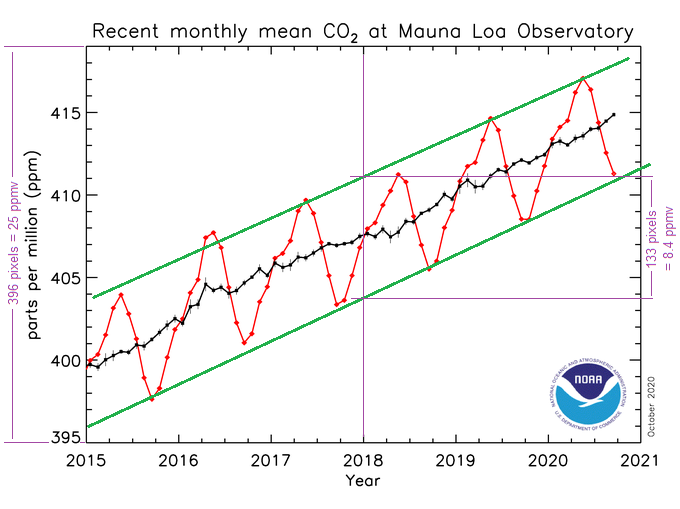
At higher northern latitudes the seasonal swing is larger. At more southern latitudes, it is smaller. At extreme southern latitudes, the seasonal cycle is reversed (but still much weaker):

Here’s a map showing the locations of Mauna Loa and Cape Grim:

I’m not saying that it is impossible to detect a 0.225 ppmv perturbation, but it definitely isn’t easy. I think you’d need to start by trying to remove other, comparable-sized influences, like ENSO.
Note: The CO2 seasonal cycle at Mauna Loa peaks in May of each year, which is why, every May/June, like clockwork, we see see a flurry of “news” stories, from the usual propaganda outlets, like The Washington Post and NOAA, about CO2 reaching a record high level.
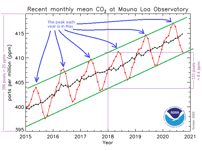
Dave,
What are the known mechanism that produce these natural variations? Are they adequately quantified?
If an emissions reduction of 10% over 6 months does not make a visible dent, how are regulators going to measure the results of mposing reduced emissions? Ordering another global 10% reduction (were that possible) would increase the risk of armed warfare within and between countries. So the regulators need to get it right. But how will they know?
Geoff S
Geoff, no, the mechanisms are not well understood. They are presumably due to a combination of biological processes, and ocean surface water temperature variations.
There tends to be an uptick in CO2 during El Ninos, e.g., that big 3.41 ppmv jump in 2016.
Extremely large volcanoes (esp. Pinetubo!) produce temporary reductions in the rate of CO2 increase, as you can see here:
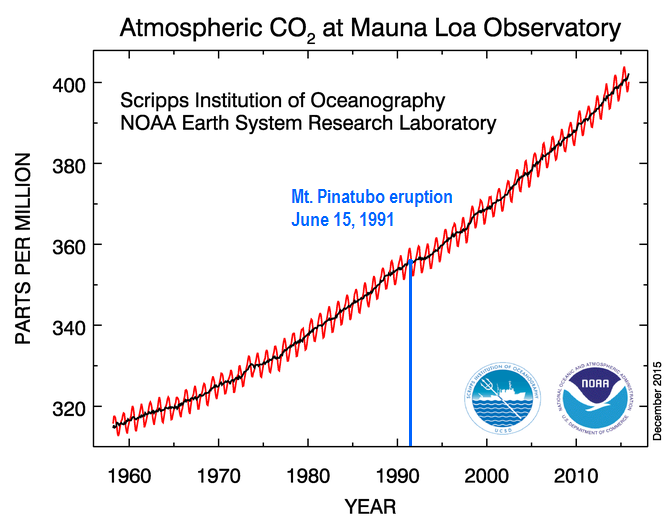
The effect of El Nino is probably at least partially due to the temperature dependence of Henry’s Law, because an El Nino causes a big patch of warm surface water in the Pacific. However, ENSO cycles have large regional effects on rainfall patterns and fisheries, which could also affect rates of natural CO2 emission and uptake.
The effect from large volcanoes might be due to aerosol/particulate cooling of ocean surface water, and/or perhaps because iron and other minerals in the volcanic ash fertilized the ocean and thereby increased CO2 uptake by ocean biota (Sarmiento, 1993 [pdf]), and/or perhaps because of the effects of sunlight scattering on vegetation growth (Farquhar & Roderick, 2003 [pdf]).
bigoilbob
You wrote above that “FFS, folks, whether you’re whining about normal measurement error or transient, correctable (and mostly corrected) systemic measurement biases, they ALL go away, as a practical matter, when considering regional/world wide changes over climactic physically/statistically significant time periods.”
They do not all go away. You are quite incorrect to assume that and I will give yopu a first-hand example to chew over.
In my younger years I owned an analytical chemistry lab, so my ability to feed my growing family depended on my performance. Performance was advertized by labs like ours and you lost clients if they found you performing worse than advertized. So, we spent a lot of time on concepts and practices of quality control errors of accuracy and precision and uncertainty.
The big show in town at the time was analysis of moon rocks and soils from programs like Apollo 11. A few dozen labs were initially chosen to receive small lots of this expensive material. They were selected on reputation and esteem. Almost all were from universities or government agencies. Besides, they tended to have the most expensive and hard-to-get equipment, like nuclear reactors to do neutron activation analysis.
When the first results came in, shiock horror, there were quite a few cases where a lab’s result was rather different to another or a group of others, beyond the boundaries of how good its performance claimes were. There were labs making errors of accuracy, one different to the next, beyond their claimed precision or advertised scatter based on repeated analysis of lots of the same material.
These errors do not go away. The reults, in theory, can be made to converge if one or more – even all – of the labs make adjustments to their methods. These adjustments are hard to design because often you do not know what causes the error and more importantly, nobody knows the “right” answer.
Over the course of time, instruments have improved. Electronics, for example, are far more stable than in the 1970s. Accuracy might have improved overall, one hopes so – but we still have the problem that a lab operating in isolation has no idea of what the right answer is. Such labs cannot improve their accuracy by doing multiple analysis of a constant material.
Coming back to GCMs and their problems, none of them knows what the right answer is. Some answers can get accepted as ok to work with when critics can find no objections to the methods and their execution. In other cases, to gain a continued living, modellers can converge on some critical values through a consent like process that might run in the mind like “All the other guys are getting a value of XYZ, a bit higher than mine. If I wind down this calibration here, mine fall into line and I can add my XYZ to the pool. This is what happens to real humans in real life. Sad, but true. It is not felt to be cheating or anti-science, it is a normal human herd response who consequences can be so trivial that nobody can really object.
All through this business of errors and GCMs, Pat Frank has been correct with his assertions and calculations. Proof is that nobody has shown him to be incorrect. That is not an absolute test, but it is a good one.
Half the time I read “CMIP6” as “Chimps”, and the rest of the time I read it as “Chips”.
Now I’m hungry.
Me too, especially when it was CMIP5.
Thanks Dr Frank, again for taking us carefully through the maze of error v uncertainty; it bells the cat of predicted CATastrophic atmospheric warming;
I also see the statistics urge to deal with randomly distributed readings using a presumption of a normally distributed variable :
I can also see uncertainty in iterative processes is at least additive –
I wonder if there is another good simple analogy that can unlock the ‘hole’ that people put themselves in – Thanks to Jim Gorman for his explanations.
The modelled prediction of warming is not an empirical data point:
I need to say it over and over
In Kansas we have the odd windy day
Thanks, Dorothy.
Models can’t predict what will happen with CO2, if anything. All the data show the behavior of the modern climate is indistinguishable from natural variability.
Everyone should feel comfortable, and just go about the business of their lives.
A later WUWT post seems to show seriously cold weather heading your way. So, see to your battening down. Stay safe and ready your galoshes. 🙂
Most of the comments are in favor. Are you here to cheerlead? A lot other issues are brought up.
The next step is to remove the error that is said to exist.
The next step is to move this theory to other models and tell why they don’t work.
In a simple game, damage done has a bell curve distribution. Who expects to do damage for the whole sequence of the fight only more than 2 standard deviations above the average? Someone that’s going to lose.
Ragnaar, you haven’t read the original paper, have you. It’s not just this one model.
Take a look at Boucher, et al., 2020, Figure 18. All the CMIP6 models make significant long wave cloud forcing (LWCF) simulation errors.
The CMIP6 average annual rms error is ±2.7 W/m^2. And that’s not a base state error. It’s the average annual calibration uncertainty in simulated LWCF across every single year of a simulated climate.
The fact that every model makes a LWCF error of different magnitude, by the way, reveals the variable parameterization sets the models have had installed by hand, so as to tune them to known target observables. The whole effort is a kludge.
If you plot a “Drunk Walk” with a random number between plus & minus 2.7 seeded with zero and 80 iterations (by 2100) it can quickly go off scale. Or is there some tendency toward zero?
The ±2.7 W/m^2 isn’t error, Steve, it’s uncertainty. So there’s no random walk of that number.
The model physics has boundary conditions, so its simulation errors can’t make it run off to infinity. The climate is physically bounded, so it’ll stay within a certain range of states.
One can’t know the errors in a futures projection. But one can know, from the presence of model calibration errors, that simulation errors will cause the predicted climate to do a random walk in the simulation phase space, away from the physically correct solution.
It’s just that the sign and magnitude of the physical errors in the predicted future climate are unknown. So, one needs an alternative reliability metric. That’s where propagation of the calibration error statistic comes into use.
Thanks for the reply – I’ll have to run through it a few times to see if I get the gist of what it is that you are saying. (-:
Why wouldn’t the best case be 10 feet exactly? Not likely, but still possible, ergo the best case.
Dave,
What are the known mechanism that produce these natural variations? Are they adequately quantified?
If an emissions reduction of 10% over 6 months does not make a visible dent, how are regulators going to measure the results of mposing reduced emissions? Ordering another global 10% reduction (were that possible) would increase the risk of armed warfare within and between countries. So the regulators need to get it right. But how will they know?
Geoff S
See https://wattsupwiththat.com/2020/10/27/cmip6-update/#comment-3114145
Pat Frank, thank you for this update. I greatly appreciate that you have so effectively followed a formal analysis from the acknowledged cloud fraction error to its necessary conclusion about uncertainty, and have stayed with that conclusion against such vehement disagreement from those who should know better. I look forward to your analysis of the temperature record. It is worth it to keep pressing on.
Thanks, David. Your encouragement is greatly appreciated, really and truly.
Pat,
Did yu see my comment above how increased model resolution does not help if there is a large continuum error
exactly as you stated.
Jerry
Hi Jerry — yes, I did see it, thanks. And, as usual with your posts, I learned something from it.
One is that I should read your papers more carefully (and probably several times). 🙂
The other is I didn’t realize that the continuum errors in the physical parameterizations that are hidden using hyperviscosity are apparently the major source of model error; at least as regards simulation of short- and medium term atmospheric dynamics.
One question that occurred to me is, if models are repaired along the lines your described, presumably weather forecasting would become more accurate and reliable over longer terms. Is that right?
But how far out do you think climate simulations could go before becoming unreliable? Would the resolution of climate models improve enough to predict the effect of the 0.035 W/m^2 annual perturbation of GHG’s?
Pat,
Although we have now pointed out the correct dynamical equations that must be used, the observational and parameterization errors are so large as to overwhelm an extended weather forecast. It has been demonstrated that inserting perfect large scale data periodically in a standard turbulence model will eventually reproduce the correct smaller scales of motion starting only from the correct large scale initial data.
This is essentially the process the weather forecasters are using when inserting new large scale data every few hours. But they do not have perfect large scale data or forcing (parameterizations).
Your analysis holds for longer term integrations. In a hyperbolic system started with perfect data at time 0 but with a continuum error ( in the equations, forcing, or numerical error) there will be an error in the solution at a later time t1.
Now start the system up at that time and there is an error in the initial data
plus any of the errors mentioned above are still there in the ensuing solution.
There are many examples that the accuracy of numerical solutions compared to a known solution deteriorates over time just from truncation errors in agreement
with your analysis.
Jerry
If I might be so bold as to offer a short quote from Dr. Taylor’s exposition on uncertainty analysis:
“In the basic sciences, error analysis has an even more fundamental role. When any new theory is proposed, it must be tested against older theories by means of one or more experiments for which the new and old theories predict different outcomes. In principle, a researcher simply performs the experiment and lets the outcome decide between the rival theories. In practice, however, the situation is complicated by the inevitable experimental uncertainties. These uncertainties must all be analyzed carefully and their effects reduced until the experiment singles out ne acceptable theory. That is, the experimental results, with their uncertainties, must be consistent with the predictions of one theory and inconsistent with those of all known, reasonable alternatives. Obviously, the success of such a procedure depends critically on the scientist’s understanding of error analysis and ability to convince others of this understanding.”
Since none of the model authors bother to do an uncertainty analysis of the inputs to their models let alone a summary uncertainty analysis of their outputs, how are the models supposed to be separated out to determine one acceptable theory? The wide spread of results from the various models would seem to indicate to an impartial judge that none of them provide a match to actual reality – meaning none of the theories (i.e. models) are acceptable predictors of the future.
The fact that so many climate scientists are un-accepting of uncertainty analysis of an iterative process is a prime indicator that they are themselves unsure of the ability of their models to predict the future. Ranting and raving about “denial” is an emotional argument, not a rational, logical argument.
That quote is on page 7 of my 2nd Edition, Tim, which just arrived yesterday. 🙂
Here’s a quote from page 6, which goes right to the heart of the climate model problem, “Note next that the uncertainty in George’s measurement is so large that his results are of no use.”
CMIP5/CMIP6 air temperature projections in a nutshell.