Plausible scenarios for climate change: 2020-2050

Reposted from Dr. Judith Curry’s Climate Etc.

Posted on February 13, 2020 by curryja |

by Judith Curry

A range of scenarios for global mean surface temperature change between 2020 and 2050, derived using a semi-empirical approach. All three modes of natural climate variability – volcanoes, solar and internal variability – are expected to act in the direction of cooling during this period.

In the midst of all the angst about 1.5^oC or 2.0^oC warming or more, as defined relative to some mythical time when climate was alleged to be ‘stable’ and (relatively) uninfluenced by humans, we lose sight of the fact that we have a better baseline period – now. One advantage of using ‘now’ as a baseline for future climate change is that we have good observations to describe  the climate of  ‘now’.

While most of the focus of climate projections is on 2100, the period circa 2020-2050 is of particular importance for several reasons:

1. It is the period for meeting UNFCCC targets for emissions reductions
2. Many financial and infrastructure decisions will be made on this time scale
3. The actual evolution of the climate over this period will influence 1) and 2) above; ‘surprises’ could have adverse impacts on decisions related to 1) and 2).

Global climate/earth system models have little skill on decadal time scales. To address this issue, CMIP5 and CMIP6 are conducting initialized, decadal scale simulations out to 35 years. While I haven’t seen any CMIP6 decadal results yet, I do follow this literature. Punchline is that there is some skill in simulating the Atlantic Multidecadal Oscillation (AMO) out to 8-10 years, but otherwise not much overall skill.

I have previously criticized the interpretation CMIP5 simulations as actual climate change scenarios – instead, these simulations show the sensitivity of climate to different emissions scenarios. They neglect scenarios of future solar variability, volcanic eruptions, and the correct phasing and amplitude of multidecadal variability associated with ocean circulations. The argument for dismissing these factors is that they are smaller than emissions forcing. Well, cumulatively and on decadal to multi-decadal timescales, this is not necessarily true.

And in the CMIP6 era, we now have sufficient information and understanding so that we can generate plausible scenarios of volcanic and solar forcing for the 21st century, as well as for the AMO.

I have developed a semi-empirical approach to formulating 21^st century climate change scenarios that rely only indirectly on climate models. Multiple scenarios are generated for each driver of the forecast (natural and anthropogenic), with an emphasis on plausible scenarios (rather than extreme scenarios that cannot completely be ruled out).

Note: in what follows, many references are cited. I don’t have time now to pull together a full bibliography, but I have provided hyperlinks to the key references.

Manmade global warming

The approach used here is to use as much as possible the new information becoming available for CMIP6: new emission scenarios, new considerations regarding climate model sensitivity to CO₂.

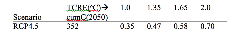
Similar to the recent IPCC SR1.5 Report, no attempt is made to use CMIP6 Earth System Model outputs. Following the IPCC SR1.5, scenarios of global warming are driven by scenarios of cumulative emissions. The individual cumulative emission scenarios between 2020 and 2050 are then translated into a global temperature increase using a range of values of the Transient Climate Response to Cumulative Carbon Emissions (TCRE). This approach is illustrated in the following figure:

Figure 1: CO2-induced warming as a function of cumulative emissions and TCRE. Millar et al

Emissions scenarios

For the forthcoming IPCC AR6, a new set of emissions scenarios (SSP) have been issued.

The 2019 World Energy Outlook Report from the International Energy Agency (IEA) challenges the near term SSP scenario projections through 2040. They examined three scenarios: a current policy scenario (CPS) where no new climate or energy policies are enacted by countries, a stated policies scenario (STPS) where Paris Agreement commitments are met, and a sustainable development scenario (SDS) where rapid mitigation limits late 21^st warming to well below 2°C. Both the IEA CPS and STPS scenarios can be considered as business-as-usual where either current policies or current commitments continue, but no additional climate policies are adopted after that point.

Figure 2 compares the IEA fossil fuel emissions projections to scenarios being used in the IPCC AR6. The figure indicates that the IEA CPS emissions are between the SSP2- RCP4.5 and SSP4-RCP6.0 scenarios and the IEA STPS scenario is slightly below SSP2-RCP4.5.

Figure 2: Annual CO2 emissions from fossil fuel and industry in CPS and STPS IEA scenarios compared to the range of baseline scenarios examined in the SSP Database, as well as a subset of the baseline and mitigation scenarios chosen for use in the forthcoming IPCC AR6 report. Ritchie and Hausfather (2019) https://thebreakthrough.org/issues/energy/3c-world

In view of these considerations, I select a single scenario for consideration here: SSP2-4.5. For the timescale of this analysis (2020-2050), there is little difference between 4.5 and 6.0, and we are not currently on the 7.0 trajectory.

Cumulative emissions for SSP2-4.5 calculated from 2020 to 2050 are reported in Table 1 for both cumulative CO₂ and cumulative C (carbon). Cumulative C is used in calculating the transient climate response to cumulative carbon emissions (TCRE); note that 1000 GtC is the carbon content of 3667 GtCO_2.

Table 1: Projections of cumulative CO₂ (GtCO₂) and C concentrations (GtC) between 2020-2050, for 3 SSP emissions scenarios. Data from IIASA database.

For reference, the IPCC SR1.5 Report assessed that amount of additional cumulative CO₂ emissions (50^th percentile) from a reference period 2006-2015 to keep additional warming to within 0.5°C is 580 GtCO₂, and to keep additional warming to within 1.0°C is 1500 GtCO₂.

TCRE

Translating the emissions scenarios into a global temperature increase has traditionally been conducted using global climate or earth system model simulations. However, the CMIP6 simulations using the new SSP scenarios and their analysis are currently underway. The recent IPCC SR1.5 Report chose to use values of the transient climate response to cumulative carbon emissions, or TCRE, to relate global temperature change to the cumulative emissions in the SSP scenarios.

The amount of warming the world is projected to experience from emissions is approximately linearly proportional to cumulative carbon emissions (for an overview, see Matthews et al. 2018). This relationship between temperatures and cumulative emissions is referred to as the transient climate response to cumulative carbon emissions, or TCRE. For a give value of TCRE, we can calculate the amount of warming expected over a future period in response to scenarios of cumulative carbon emission.

The IPCC AR5 provided a likely range for TCRE of 0.8°C to 2.5°C. Matthews et al. (2018) state that the current generation of full-complexity Earth-system models exhibits a range of TCRE values of between 0.8 and 2.4°C, with a median value of 1.6°C. An observationally-constrained TCRE estimate gave a 5%–95% confidence range of 0.7 −2.0°C, with a best-estimate of 1.35 ◦C (Gillett et al 2013). A more recent observationally-constrained estimate is provided by Lewis (2018), who determined a best estimate of 1.05°C.

In view of these assessments, I select the following values of TCRE for scenarios: 1.0, 1.35, 1.65, 2.0°C as constituting a range of plausible values.

Table 2 provides calculations of the amount of warming between 2020 and 2050, based on SSP2-4.5 and four values of TCRE. As expected from the range of TCRE values used here, there is a factor-of-two range in the amount of emissions-driven warming expected for the period 2020-2050.

Table 2: Warming scenarios (^oC) for 2050 from a 2020 baseline based on the SSP2-4.5 cumulative emissions scenario (GtC) and four values of TCRE (^oC)

Projections of natural climate variability

Scenarios of future variations/changes are presented for 2030-2050 for the following:

• Solar variations
• Volcanic eruptions
• Decadal-scale ocean circulation variability

Solar variations

With regards to solar scenarios for the 21^st century, there are two issues:

• How much total solar insolation (TSI) will change
• How much warming, given a specific TSI.

According to the IPCC AR5, the influence of the Sun on our climate since pre-industrial times, in terms of radiative forcing, is very small compared to the variation of radiative forcing due to added anthropogenic greenhouse gases: 0.05 W/m² vs. 2.29 W/m². Thus, the IPCC AR5 message is that changes in solar activity are nearly negligible compared to anthropogenic forcing.

This interpretation has been challenged:

• There is substantial disagreement on trends in solar activity, even in the satellite era. Several papers in the last decade have claimed that solar activity in the second part of the 20^th century was higher than any time in the past 10,000 years. Some studies claim that the Sun could have contributed at least ∼ 50% of the post 1850 global warming.
• The IPCC AR5 considered only the direct solar effects on global temperatures. It has been found that over the eleven- year solar cycle the energy that enters the Earth’s system is of the order of 1.0–1.5 W/m². This is almost an order of magnitude larger than what would be expected from solar irradiance alone, and suggests that solar activity is getting amplified atmospheric processes. Candidate processes include: solar ultraviolet changes; energetic particle precipitation; atmospheric-electric-field effect on cloud cover; 
cloud changes produced by solar-modulated galactic cosmic rays; large relative changes in its magnetic field; strength of the solar wind.
• The relations between solar variations and Earth climate are many and complicated. Most of them work locally and regionally, and many are non-linear. Strong solar influences have been seen in the Pacific and Indian Oceans and also in the Arctic, among other regions.

As summarized by Svensmark (2019), satellite data demonstrate that TSI varies by as much as 0.05–0.07% over a solar cycle. At the top of the atmosphere this variation amounts to around 1 W/m2 out of a solar constant of around 1361 W/m2. At the surface, this is only 0.2 W/m2, after taking geometry and albedo into account. Model simulations and observations have shown a response of global surface temperature to TSI variations over the 11-year solar cycle of about 0.1^oC (Matthes et al. 2017).

The current solar cycle 24 is the smallest sunspot cycle in 100 years and the third in a trend of diminishing sunspot cycles. Is the Sun is currently moving into a new grand minimum or just a period of low solar activity? Many solar physicists expect the sun to move into a new minimum during the 21^st century: a century-level low, although several predict a minimum comparable with the Dalton or even the Maunder Minimum.

In CMIP5, climate projections were based on a stationary-Sun scenario, obtained by simply repeating solar cycle 23, which ran from April 1996 to June 2008, which is the third strongest solar cycle since 1850. Clearly, such a stationary scenario is not representative of true solar activity, which exhibits cycle-to-cycle variations and trends. Therefore, in CMIP6 more realistic scenarios were developed for future solar activity, exhibiting variability at all timescales (Matthes et al. 2017). Matthes et al. present the following two scenarios (Figure 3): a reference scenario and a Maunder minimum scenario for the second half of the 21^st century.

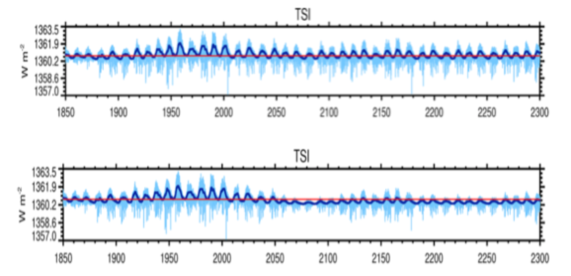
Figure 3: CMIP6 scenarios for solar forcing (TSI): reference scenario (top); Maunder minimum scenario (bottom). Matthes et al. (2017)

If a Maunder minimum-scale event were to occur in the 21^st century, how much cooling would this cause? As summarized by Svensmark (2019), a majority of reconstructions find only small changes in overall secular solar radiative output: since the Maunder Minimum, TSI is believed to have increased by around 1 W/m2, which corresponds to 0.18 W/m2 at the Earth’s surface – this is the same magnitude of the amplitude of the 11 year solar cycle. Jones et al. (2012) used a simple climate model to estimate that the likely reduction in the warming by 2100 from a ‘Maunder minimum’ scale event to be between 0.06 and 0.1 °C. Fuelner and Rahmstorf (2010) estimated that another solar minimum equivalent to the Dalton and Maunder minima would cause 0.09°C and 0.26°C cooling, respectively. Meehl et al. (2013) estimated a Maunder minimum cooling of 0.3°C.

These calculations ignored any indirect solar effects, which would arguably increase these numbers by up to a factor of 3 to 7. Shaviv (2008) used the oceans as a calorimeter to measure the radiative forcing variations associated with the solar cycle. Shaviv found that the energy that enters the oceans over a solar cycle is 5–7 times larger than the 0.1% change in TSI, thus implying the necessary existence of an amplification mechanism. Scafetta (2013) showed that the large climatic variability observed since the medieval times can be correctly interpreted only if the climatic effects of solar variability on the climate have been severely underestimated by the climate models by a 3 to 6 factor. Svensmark (2019) made a comparable argument using borehole temperatures for the period since the Medieval Warm Period, finding an amplification of a factor of 5 to 7 over the warming expected from a drop in TSI. If an amplification factor is included of these magnitudes, then a surface temperature decrease of up to 1^oC (or even more) from a Maunder minimum could be expected.

Three scenarios for solar variability are used here:

• No variability (CMIP5)
• CMIP6 reference scenario, with factor of two amplification by solar indirect effects
• CMIP6 Maunder Minimum scenario, with factor of four amplification by solar indirect effects (note: the period 2020-2050 has lower values of TSI than the reference scenario, but the actual Minimum is in the latter half of the 21^st century).

Note: the CMIP6 values of changes in TSI are ‘eyeballed’ from Figure 3 (I did not download the CMIP6 solar projections). I would greatly appreciate other interpretations of the values of surface cooling to infer from the CMIP6 solar scenarios.

Table 3. Scenarios of solar cooling (^oC), relative to the CMIP5 solar cycle

Volcanoes

The 21^st century CMIP5 climate model simulations did not include any radiative forcing from future volcanic eruptions. While volcanic eruptions are not predictable, a scenario of zero radiative forcing from volcanoes in the 21^st century is a poor assumption. Further, assuming a repeat of the 20^th century volcanic radiative forcing is not a very good assumption, either.

In the past decade, there have been two major paleoclimate reconstructions of volcanic eruptions in the recent millennia. Gao et al. (2008) examined ice core records and their following reconstruction for sulfate ejection from volcanic eruptions. A more recent reconstruction by Sigl et al. (2015) is provided below, presented in terms of global volcanic aerosol radiative forcing. These reconstructions put into perspective the relative low level of volcanic activity since the mid 19^th century.

Figure 4: Reconstruction of global volcanic aerosol radiative forcing for the past 2500 years. Sigl et al. (2015)

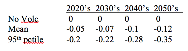
Because volcanic eruptions are unpredictable events, they have generally been excluded from twenty-first century climate projection protocols. Most recent projections either specify future volcanic forcing as zero or a constant background value. Bethke et al. (2017) explored how sixty possible volcanic futures, consistent with ice-core records, impact climate variability projections of the Norwegian Earth System Model (NorESM; ECS=3.2C) under RCP4.5. Clustered occurrence of strong tropical eruptions has contributed to sustained cold periods such as the Little Ice Age, where the longer- term climate impacts are mediated through ocean heat content anomalies and ocean circulation changes. Extreme volcanic activity can potentially cause extended anomalously cold periods.

Figure 5: Annual-mean GMST. Ensemble mean (solid) of VOLC (stochastic volcanic forcing; blue), VOLC-CONST (average 1850-2000 volcanic forcing; magenta) and NO-VOLC (red/orange) with 5–95% range (shading) and ensemble minima/maxima (dots) for VOLC and NO-VOLC; evolution of the most extreme member (black). Bethke et al. (2017).

Based on the results of Bethke et al. (2017), three volcanic scenarios for cooling are used, related to the decadal values shown in Figure 5:

• No forcing
• 50^th percentile value: mean forcing
• 95^th percentile value: large forcing

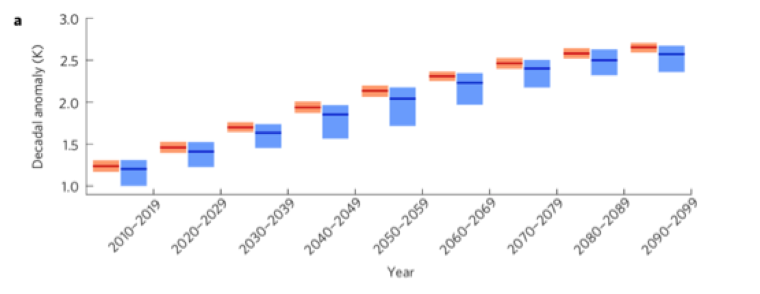
Figure 6. Decadal means of GMST relative to pre-industrial. Ensemble mean (solid) with 5–95% range (shading) of VOLC (blue) and NO-VOLC (red).

Table 4 shows the decadal scenarios of volcanic cooling, consistent with Figure 6.

Table 4. Decadal scenarios of volcanic cooling (^oC). From Bethke et al. (2017)

Internal variability

Variations in global mean surface temperature are also associated with recurrent multi-decadal internal variability associated with large-scale ocean circulations. However, separating the internal variability from forced variability is not always straightforward owing to uncertainties in external forcing.

The multi-decadal internal variability (50-80 year band) has been estimated to have a peak-to-peak amplitude of global surface temperature as high as 0.3-0.4^oC (Tung and Zhou, 2012), accounting for about half of the late 20^th century warming. DelSole et al. (2010) estimated a peak-to-peak global temperature change of 0.24^oC from internal variability. By contrast, Stolpe (2016) estimated a maximum peak-to-peak amplitude of 0.16^oC. Knutson et al. (2016) used the GFDL CM3 model, which has strong internal multidecadal variability, to identify several periods that exceed 0.5^oC for global mean surface temperature, indicating that data records of ~160 years are too short for a full sampling of multi-decadal internal climate variability.

Most analyses have identified Atlantic Multidecadal Variability as having the dominant imprint on global and Northern Hemisphere temperatures. Identification of ENSO as a driver of global mean temperature variations or response signal remains contentious, with conflicting results. Bhaskar et al. (2017) characterizes ENSO as a secondary driver of variations in global mean temperature, accounting for 12% of variability over the last century, with ENSO and global mean surface temperature mutually driving each other at varied time lags.

Not taking multi-decadal variability into account in predictions of future warming under various forcing scenarios may run the risk of over-estimating the warming for the next two to three decades, when the Atlantic Multi-decadal Oscillation (AMO) is likely to shift into its cold phase.

Analysis of historical and paleoclimatic records suggest that a transition to the cold phase of the AMO is expected prior to 2050. Enfield and Cid-Serrano (2006) used paleoclimate reconstructions of the AMO to develop a probabilistic projection of the next AMO shift. Figure 7 shows the probability of an AMO shift relative to the number of years since the last regime shift. The previous regime shift occurred in 1995; hence in 2020, it has been 23 years since the previous shift. Figure 7 indicates that a shift to the cold phase is expected to occur within the next 15 years, with a 50% probability of the shift occurring in the next 6 years.

Figure 7. Probability of an AMO regime shift relative the number of years since the last regime shift. Source: Enfield and Cid-Serrano (2006)

The timing of a shift to the AMO cold phase is not predictable; it depends to some extent on unpredictable weather variability (Johnstone, 2020). Johnstone’s analysis shows that low-frequency changes in North Atlantic SSTs since 1880 are objectively identified as a series of alternating ‘regime shifts’ with abrupt (~1-year) transitions dated to 1902, 1926, 1971 and 1995 (Figure 8).   In the recent historical record (back to 1880), these sharp changes punctuate longer quasi-stable periods of 24 years (1902-1925), 45 years (1926-1970), and 24 years (1971-1994), while the latest, and warmest regime on record has persisted with little net change from 1995 through 2019 (25 years). Previous cool shifts in 1902 and 1971 shared similar -0.2°C amplitudes, following extended periods of relative warmth (1880-1901), (1926-1970). A negative (cool) shift within a shorter time frame (~5 years) might be tentatively inferred from a steep 2015 SST decline in the subpolar North Atlantic, behavior that might presage broader North Atlantic cooling based on early subpolar appearance of the most recent cool shift of 1971.

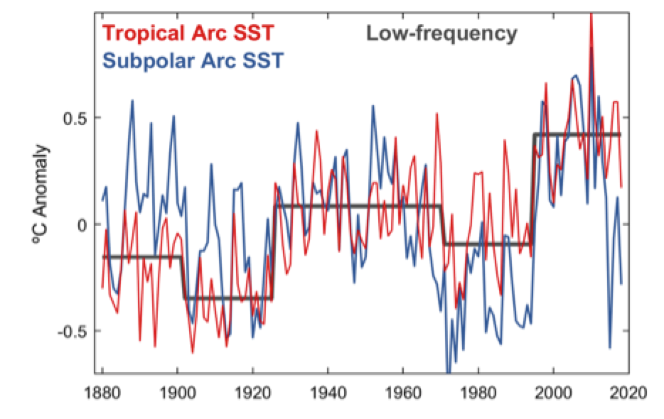
Figure 8.   Annual SST anomalies in the subpolar (blue) and tropical (red) North Atlantic. A sharp subpolar cooling is evident in 2015. Johnstone (2020)

Guided by the above analyses, three scenarios for global temperature change associated with the AMO are presented in Table 5.

Table 5. Decadal scenarios of temperature change from internal variability (^oC), associated with a transition to the cool phase of the Atlantic Multidecadal Oscillation.

Integral scenarios of temperature change: 2050

The final integral temperature change is the sum of temperature changes driven by

• Emissions (4 scenario)
• Volcanoes (3 scenarios)
• Solar (3 scenarios)
• AMO (3 scenarios)

There are 108 possible different combinations of these scenarios.  Table 6 shows extreme high and low warming scenario, plus the scenario using all of the mid range values.

Table 6. Integral scenarios of global mean surface temperature change for 2020-2050.

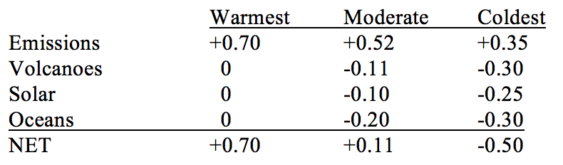
All of the components of natural variability point to cooling during the period 2020-2050. Individually these terms are not expected to be large in the moderate scenarios.   However, when summed their magnitude approaches the magnitude of the warming associated with the moderate values of TCRE – 1.35 and 1.65 ^oC. If the natural cooling exceeds the expected value, or TCRE is at the low end (1.0 to 1.35^oC), then there could be net cooling.

The possibility and probability of 21^st century decades being characterized by net cooling has been addressed by several papers. This depends on model value of ECS, and the magnitude of the predicted natural variability. Knutson et al.  (2016) used the GFDL climate model (relatively high value of ECS; high internal variability) to determine that probability of global temperature trend <0 for period of 20-30 years is 2%.  Bethke et al. (2017) used NorESM (ECS=3.2C) with RCP4.5. This paper examined the combination of scenarios of internal variability and volcanic eruptions. They found that occurrences of decades with negative GMST trend become more frequent if accounting for volcanic forcing, with the probability increasing from 10% in NO-VOLC to more than 16% in VOLC. The probability of decades with negative GMST trend more than doubles from 4% to 10% if the analysis is limited to the first half of the century—before the stabilization period of RCP4.5. Volcanic-induced cooling becomes increasingly important in facilitating neutral or negative temperature trends on longer timescales, in conjunction with natural internal variability effects.

In summary, decade(s) during the period 2020-2050 with zero warming or even cooling should not be particularly surprising.

Conclusions

Three main conclusions:

• We are starting to narrow the uncertainty in the amount of warming from emissions that we can expect out to 2050
• All three modes of natural variability – solar, volcanoes, internal variability – are expected to trend cool over the next 3 decades
• Depending on the relative magnitudes of emissions driven warming versus natural variability, decades with no warming or even cooling are more or less plausible.

If you prefer your scenarios on the high side, you can include scenarios with RCP7.0 and TCRE=2.4^oC, but these values don’t change the fundamental narrative presented here. You can also add 1.2^oC to the values in Table 6, to make the numbers look higher. But if you want plausible scenarios, look to my Table 6, which I think bounds the range of plausible outcomes for global mean surface temperature from 2020-2050.

But what about the 2^nd half of the 21^st century and 2100? Uncertainties regarding emissions are much greater in the 2^nd half of the 21^st century. The CMIP6 solar scenarios (Reference and Maunder) show more cooling in the second half of the 21^st century. Volcanic eruptions could be larger in 2^nd half of 21^st century (or not). After the projected cool phase of the AMO, a return to the warm phase is expected, but there is no confidence in projecting either a warm or cold phase AMO in 2100.

Apart from the ‘wild card’ of volcanic eruptions, the big uncertainty is solar indirect effects. Based on the literature survey that I’ve conducted, solar UV effects on climate seem to be at least as large as TSI effects. A factor of 2-4 (X TSI) seems completely plausible to me, and serious arguments have been presented for even higher values. I also note here that almost all estimates of ECS/TCR from observations do not include any allowances for uncertainties associated with solar indirect effects. Scafetta (2013) included solar indirect effects in an estimate of ECS, and determined an ECS value of 1.35 ^oC.

Neither the effects of AMO or solar indirect effects have been included in attribution analyses of warming since 1950.

So why does this analysis ‘matter’?

• For those that are urgently worried about the impacts of AGW and the need to act urgently to meet deadlines related to emissions, the natural climate variability may help slow down the warming over the next few decades, allowing for time to make prudent, cost effective decisions that make sense for the long term.
• Failure to anticipate and understand periods of stagnant warming or even cooling detract from the credibility of climate science and may diminish the ‘will to act.’

I look forward to your comments.  I encourage you to critique and check my numbers, especially related to solar.