Explaining the Discrepancies Between Hausfather et al. (2019) and Lewis&Curry (2018)

Reposted from Dr. Judith Curry’s Climate Etc.

by Ross McKitrick

Challenging the claim that a large set of climate model runs published since 1970’s are consistent with observations for the right reasons.

Introduction

Zeke Hausfather et al. (2019) (herein ZH19) examined a large set of climate model runs published since the 1970s and claimed they were consistent with observations, once errors in the emission projections are considered. It is an interesting and valuable paper and has received a lot of press attention. In this post, I will explain what the authors did and then discuss a couple of issues arising, beginning with IPCC over-estimation of CO2 emissions, a literature to which Hausfather et al. make a striking contribution. I will then present a critique of some aspects of their regression analyses. I find that they have not specified their main regression correctly, and this undermines some of their conclusions. Using a more valid regression model helps explain why their findings aren’t inconsistent with Lewis and Curry (2018) which did show models to be inconsistent with observations.

Outline of the ZH19 Analysis:

A climate model projection can be factored into two parts: the implied (transient) climate sensitivity (to increased forcing) over the projection period and the projected increase in forcing. The first derives from the model’s Equilibrium Climate Sensitivity (ECS) and the ocean heat uptake rate. It will be approximately equal to the model’s transient climate response (TCR), although the discussion in ZH19 is for a shorter period than the 70 years used for TCR computation. The second comes from a submodel that takes annual GHG emissions and other anthropogenic factors as inputs, generates implied CO2 and other GHG concentrations, then converts them into forcings, expressed in Watts per square meter. The emission forecasts are based on socioeconomic projections and are therefore external to the climate model.

ZH19 ask whether climate models have overstated warming once we adjust for errors in the second factor due to faulty emission projections. So it’s essentially a study of climate model sensitivities. Their conclusion, that models by and large generate accurate forcing-adjusted forecasts, implies that models have generally had valid TCR levels. But this conflicts with other evidence (such as Lewis and Curry 2018) that CMIP5 models have overly high TCR values compared to observationally-constrained estimates. This discrepancy needs explanation.

One interesting contribution of the ZH19 paper is their tabulation of the 1970s-era climate model ECS values. The wording in the ZH19 Supplement, which presumably reflects that in the underlying papers, doesn’t distinguish between ECS and TCR in these early models. The reported early ECS values are:

• Manabe and Weatherald (1967) / Manabe (1970) / Mitchell (1970): 2.3K
• Benson (1970) / Sawyer (1972) / Broecker (1975): 2.4K
• Rasool and Schneider (1971) 0.8K
• Nordhaus (1977): 2.0K

If these really are ECS values they are pretty low by modern standards. It is widely-known that the 1979 Charney Report proposed a best-estimate range for ECS of 1.5—4.5K. The follow-up National Academy report in 1983 by Nierenberg et al. noted (p. 2) “The climate record of the past hundred years and our estimates of CO2 changes over that period suggest that values in the lower half of this range are more probable.” So those numbers might be indicative of general thinking in the 1970s. Hansen’s 1981 model considered a range of possible ECS values from 1.2K to 3.5K, settling on 2.8K for their preferred estimate, thus presaging the subsequent use of generally higher ECS values.

But it is not easy to tell if these are meant to be ECS or TCR values. The latter are always lower than ECS, due to slow adjustment by the oceans. Model TCR values in the 2.0–2.4 K range would correspond to ECS values in the upper half of the Charney range.

If the models have high interval ECS values, the fact that ZH19 find they stay in the ballpark of observed surface average warming, once adjusted for forcing errors, suggests it’s a case of being right for the wrong reason. The 1970s were unusually cold, and there is evidence that multidecadal internal variability was a significant contributor to accelerated warming from the late 1970s to the 2008 (see DelSole et al. 2011). If the models didn’t account for that, instead attributing everything to CO2 warming, it would require excessively high ECS to yield a match to observations.

With those preliminary points in mind, here are my comments on ZH19.

There are some math errors in the writeup.

The main text of the paper describes the methodology only in general terms. The online SI provides statistical details including some mathematical equations. Unfortunately, they are incorrect and contradictory in places. Also, the written methodology doesn’t seem to match the online Python code. I don’t think any important results hang on these problems, but it means reading and replication is unnecessarily difficult. I wrote Zeke about these issues before Christmas and he has promised to make any necessary corrections to the writeup.

One of the most remarkable findings of this study is buried in the online appendix as Figure S4, showing past projection ranges for CO2 concentrations versus observations:

Bear in mind that, since there have been few emission reduction policies in place historically (and none currently that bind at the global level), the heavy black line is effectively the Business-as-Usual sequence. Yet the IPCC repeatedly refers to its high end projections as “Business-as-Usual” and the low end as policy-constrained. The reality is the high end is fictional exaggerated nonsense.

I think this graph should have been in the main body of the paper. It shows:

• In the 1970s, models (blue) had a wide spread but on average encompassed the observations (though they pass through the lower half of the spread);
• In the 1980s there was still a wide spread but now the observations hug the bottom of it, except for the horizontal line which was Hansen’s 1988 Scenario C;
• Since the 1990s the IPCC constantly overstated emission paths and, even more so, CO2 concentrations by presenting a range of future scenarios, only the minimum of which was ever realistic.

I first got interested in the problem of exaggerated IPCC emission forecasts in 2002 when the top-end of the IPCC warming projections jumped from about 3.5 degrees in the 1995 SAR to 6 degrees in the 2001 TAR. I wrote an op-ed in the National Post and the Fraser Forum (both available here) which explained that this change did not result from a change in climate model behaviour but from the use of the new high-end SRES scenarios, and that many climate modelers and economists considered them unrealistic. The particularly egregious A1FI scenario was inserted into the mix near the end of the IPCC process in response to government (not academic) reviewer demands. IPCC Vice-Chair Martin Manning distanced himself from it at the time in a widely-circulated email, stating that many of his colleagues viewed it as “unrealistically high.”

Some longstanding readers of Climate Etc. may also recall the Castles-Henderson critique which came out at this time. It focused on IPCC misuse of Purchasing Power Parity aggregation rules across countries. The effect of the error was to exaggerate the relative income differences between rich and poor countries, leading to inflated upper end growth assumptions for poor countries to converge on rich ones. Terence Corcoran of the National Post published an article on November 27 2002 quoting John Reilly, an economist at MIT, who had examined the IPCC scenario methodology and concluded it was “in my view, a kind of insult to science” and the method was “lunacy.”

Years later (2012-13) I published two academic articles (available here) in economics journals critiquing the IPCC SRES scenarios. Although global total CO2 emissions have grown quite a bit since 1970, little of this is due to increased average per capita emissions (which have only grown from about 1.0 to 1.4 tonnes C per person), instead it is mainly driven by global population growth, which is slowing down. The high-end IPCC scenarios were based on assumptions that population and per capita emissions would both grow rapidly, the latter reaching 2 tonnes per capita by 2020 and over 3 tonnes per capita by 2050. We showed that the upper half of the SRES distribution was statistically very improbable because it would require sudden and sustained increases in per capita emissions which were inconsistent with observed trends. In a follow-up article, my student Joel Wood and I showed that the high scenarios were inconsistent with the way global energy markets constrain hydrocarbon consumption growth. More recently Justin Ritchie and Hadi Dowladabadi have explored the issue from a different angle, namely the technical and geological constraints that prevent coal use from growing in the way assumed by the IPCC (see here and here).

IPCC reliance on exaggerated scenarios is back in the news, thanks to Roger Pielke Jr.’s recent column on the subject (along with numerous tweets from him attacking the existence and usage of RCP8.5) and another recent piece by Andrew Montford. What is especially egregious is that many authors are using the top end of the scenario range as “business-as-usual”, even after, as shown in the ZH19 graph, we have had 30 years in which business-as-usual has tracked the bottom end of the range.

In December 2019 I submitted my review comments for the IPCC AR6 WG2 chapters. Many draft passages in AR6 continue to refer to RCP8.5 as the BAU outcome. This is, as has been said before, lunacy—another “insult to science”.

Apples-to-apples trend comparisons requires removal of Pinatubo and ENSO effects

The model-observational comparisons of primary interest are the relatively modern ones, namely scenarios A—C in Hansen (1988) and the central projections from various IPCC reports: FAR (1990), SAR (1995), TAR (2001), AR4 (2007) and AR5 (2013). Since the comparison uses annual averages in the out-of-sample interval the latter two time spans are too short to yield meaningful comparisons.

Before examining the implied sensitivity scores, ZH19 present simple trend comparisons. In many cases they work with a range of temperatures and forcings but I will focus on the central (or “Best”) values to keep this discussion brief.

ZH19 find that Hansen 1988-A and 1988-B significantly overstate trends, but not the others. However, I find FAR does as well. SAR and TAR don’t but their forecast trends are very low.

The main forecast interval of interest is from 1988 to 2017. It is shorter for the later IPCC reports since the start year advances. To make trend comparisons meaningful, for the purpose of the Hansen (1988-2017) and FAR (1990-2017) interval comparisons, the 1992 (Mount Pinatubo) event needs to be removed since it depressed observed temperatures but is not simulated in climate models on a forecast basis. Likewise with El Nino events. By not removing these events the observed trend is overstated for the purpose of comparison with models.

To adjust for this I took the Cowtan-Way temperature series from the ZH19 data archive, which for simplicity I will use as the lone observational series, and filtered out volcanic and El Nino effects as follows. I took the IPCC AR5 volcanic forcing series (as updated by Nic Lewis for Lewis&Curry 2018), and the NCEP pressure-based ENSO index (from here). I regressed Cowtan-Way on these two series and obtained the residuals, which I denote as “Cowtan-Way adj” in the following Figure (note both series are shifted to begin at 0.0 in 1988):

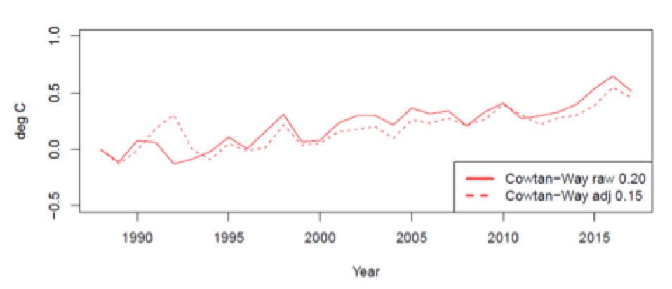
The trends, in K/decade, are indicated in the legend. The two trend coefficients are not significantly different from each other (using the Vogelsang-Franses test). Removing the volcanic forcing and El Nino effects causes the trend to drop from 0.20 to 0.15 K/decade. The effect is minimal on intervals that start after 1995. In the SAR subsample (1995-2017) the trend remains unchanged at 0.19 K/decade and in the TAR subsample (2001-2017) the trend increases from 0.17 to 0.18 K/decade.

Here is what the adjusted Cowtan-Way data looks like, compared to the Hansen 1988 series:

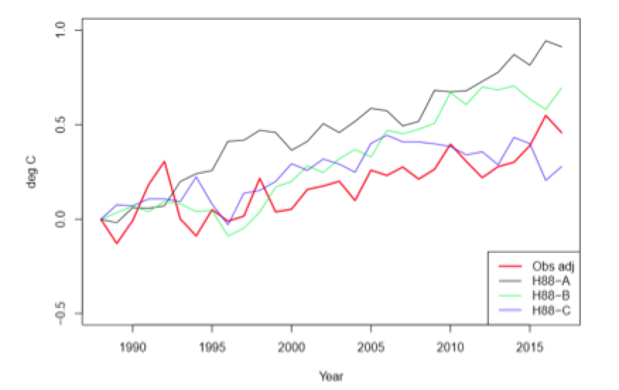
The linear trend in the red line (adjusted observations) is 0.15 C/decade, just a bit above H88-C (0.12 C/decade) but well below the H88-A and H88-B trends (0.30 and 0.28 C/decade respectively)

The ZH19 trend comparison methodology is an ad hoc mix of OLS and AR1 estimation. Since the methodology write-up is incoherent and their method is non-standard I won’t try to replicate their confidence intervals (my OLS trend coefficients match theirs however). Instead I’ll use the Vogelsang-Franses (VF) autocorrelation-robust trend comparison methodology from the econometrics literature. I computed trends and 95% CI’s in the two CW series, the 3 Hansen 1988 A,B,C series and the first three IPCC out-of-sample series (denoted FAR, SAR and TAR). The results are as follows:

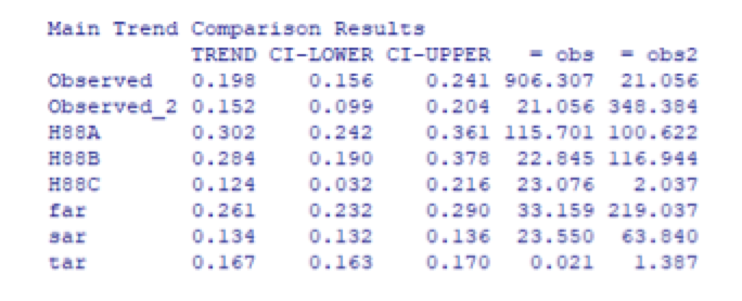
The OLS trends (in K/decade) are in the 1^st column and the lower and upper bounds on the 95% confidence intervals are in the next two columns.

The 4^th and 5^th columns report VF test scores, for which the 95% critical value is 41.53. In the first two rows, the diagonal entries (906.307 and 348.384) are tests on a null hypothesis of no trend; both reject at extremely small significance levels (indicating the trends are significant). The off-diagonal scores (21.056) test if the trends in the raw and adjusted series are significantly different. It does not reject at 5%.

The entries in the subsequent rows test if the trend in that row (e.g. H88-A) equals the trend in, respectively, the raw and adjusted series (i.e. obs and obs2), after adjusting the sample to have identical time spans. If the score exceeds 41.53 the test rejects, meaning the trends are significantly different.

The Hansen 1988-A trend forecast significantly exceeds that in both the raw and adjusted observed series. The Hansen 1988-B forecast trend does not significantly exceed that in the raw CW series but it does significantly exceed that in the adjusted CW (since the VF score rises to 116.944, which exceeds the 95% critical value of 41.53). The Hansen 1988-C forecast is not significantly different from either observed series. Hence, the only Hansen 1988 forecast that matches the observed trend, once the volcanic and El Nino effects are removed, is scenario C, which assumes no increase in forcing after 2000. The post-1998 slowdown in observed warming ends up matching a model scenario in which no increase in forcing occurs, but does not match either scenario in which forcing is allowed to increase, which is interesting.

The forecast trends in FAR and SAR are not significantly different from the raw Cowtan-Way trends but they do differ from the adjusted Cowtan-Way trends. (The FAR trend also rejects against the raw series if we use GISTEMP, HadCRUT4 or NOAA). The discrepancy between FAR and observations is due to the projected trend being too large. In the SAR case, the projected trend is smaller than the observed trend over the same interval (0.13 versus 0.19). The adjusted trend is the same as the raw trend but the series has less variance, which is why the VF score increases. In the case of CW and Berkeley it rises enough to reject the trend equivalence null; if we use GISTEMP, HadCRUT4 or NOAA neither raw nor adjusted trends reject against the SAR trend.

The TAR forecast for 2001-2017 (0.167 K/decade) never rejects against observations.

So to summarize, ZH19 go through the exercise of comparing forecast to observed trends and, for the Hansen 1988 and IPCC trends, most forecasts do not significantly differ from observations. But some of that apparent fit is due to the 1992 Mount Pinatubo eruption and the sequence of El Nino events. Removing those, the Hansen 1988-A and B projections significantly exceed observations while the Hansen 1988 C scenario does not. The IPCC FAR forecast significantly overshoots observations and the IPCC SAR significantly undershoots them.

In order to refine the model-observation comparison it is also essential to adjust for errors in forcing, which is the next task ZH19 undertake.

Implied TCR regressions: a specification challenge

ZH19 define an implied Transient Climate Response (TCR) as

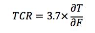
where T is temperature, F is anthropogenic forcing, and the derivative is computed as the least squares slope coefficient from regressing temperature on forcing over time. Suppressing the constant term the regression for model i is simply

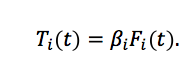
The TCR for model i is therefore where 3.7 (W/m²) is the assumed equilibrium CO2 doubling coefficient. They find 14 of the 17 implied TCR’s are consistent with an observational counterpart, defined as the slope coefficient from regressing temperatures on an observationally-constrained forcing series.

Regarding the post-1988 cohort, unfortunately ZH19 relied on an ARIMA(1,0,0) regression specification, or in other words a linear regression with AR1 errors. While the temperature series they use are mostly trend stationary (i.e. stationary after de-trending), their forcing series are not. They are what we call in econometrics integrated of order 1, or I(1), namely the first differences are trend stationary but the levels are nonstationary. I will present a very brief discussion of this but I will save the longer version for a journal article (or a formal comment on ZH19).

There is a large and growing literature in econometrics journals on this issue as it applies to climate data, with lots of competing results to wade through. On the time spans of the ZH19 data sets, the standard tests I ran (namely Augmented Dickey-Fuller) indicate temperatures are trend-stationary while forcings are nonstationary. Temperatures therefore cannot be a simple linear function of forcings, otherwise they would inherit the I(1) structure of the forcing variables. Using an I(1) variable in a linear regression without modeling the nonstationary component properly can yield spurious results. Consequently it is a misspecification to regress temperatures on forcings (see Section 4.3 in this chapter for a partial explanation of why this is so).

How should such a regression be done? Some time series analysts are trying to resolve this dilemma by claiming that temperatures are I(1). I can’t replicate this finding on any data set I’ve seen, but if it turns out to be true it has massive implications including rendering most forms of trend estimation and analysis hitherto meaningless.

I think it is more likely that temperatures are I(0), as are natural forcings, and anthropogenic forcings are I(1). But this creates a big problem for time series attribution modeling. It means you can’t regress temperature on forcings the way ZH19 did; in fact it’s not obvious what the correct way would be. One possible way to proceed is called the Toda-Yamamoto method, but it is only usable when the lags of the explanatory variable can be included, and in this case they can’t because they are perfectly collinear with each other. The main other option is to regress the first differences of temperatures on first differences of forcings, so I(0) variables are on both sides of the equation. This would imply an ARIMA(0,1,0) specification rather than ARIMA(1,0,0).

But this wipes out a lot of information in the data. I did this for the later models in ZH19, regressing each one’s temperature series on each one’s forcing input series, using a regression of Cowtan-Way on the IPCC total anthropogenic forcing series as an observational counterpart. Using an ARIMA(0,1,0) specification except for AR4 (for which ARIMA(1,0,0) is indicated) yields the following TCR estimates:

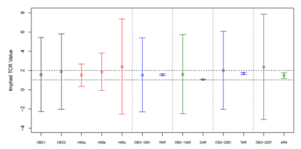
The comparison of interest is OBS1 and OBS2 to the H88a—c results, and for each IPCC report the OBS-(startyear) series compared to the corresponding model-based value. I used the unadjusted Cowtan-Way series as the observational counterparts for FAR and after.

In one sense I reproduce the ZH19 findings that the model TCR estimates don’t significantly differ from observed, because of the overlapping spans of the 95% confidence intervals. But that’s not very meaningful since the 95% observational CI’s also encompass 0, negative values, and implausibly high values. They also encompass the Lewis & Curry (2018) results. Essentially, what the results show is that these data series are too short and unstable to provide valid estimates of TCR. The real difference between models and observations is that the IPCC models are too stable and constrained. The Hansen 1988 results actually show a more realistic uncertainty profile, but the TCR’s differ a lot among the three of them (point estimates 1.5, 1.9 and 2.4 respectively) and for two of the three they are statistically insignificant. And of course they overshoot the observed warming.

The appearance of precise TCR estimates in ZH19 is spurious due to their use of ARIMA(1,0,0) with a nonstationary explanatory variable. A problem with my approach here is that the ARIMA(0,1,0) specification doesn’t make efficient use of information in the data about potential long run or lagged effects between forcings and temperatures, if they are present. But with such short data samples it is not possible to estimate more complex models, and the I(0)/I(1) mismatch between forcings and temperatures rule out finding a simple way of doing the estimation.

Conclusion

The apparent inconsistency between ZH19 and studies like Lewis & Curry 2018 that have found observationally-constrained ECS to be low compared to modeled values disappears once the regression specification issue is addressed. The ZH19 data samples are too short to provide valid TCR values and their regression model is specified in such a way that it is susceptible to spurious precision. So I don’t think their paper is informative as an exercize in climate model evaluation.

It is, however, informative with regards to past IPCC emission/concentration projections and shows that the IPCC has for a long time been relying on exaggerated forecasts of global greenhouse gas emissions.

I’m grateful to Nic Lewis for his comments on an earlier draft.

Comment from Nic Lewis

These early models only allowed for increases in forcing from CO2, not from all forcing agents. Since 1970, total forcing (per IPCC AR5 estimates) has grown more than 50% faster than CO2-only forcing, so if early model temperature trends and CO2 concentration trends over their projection periods are in line with observed warming and CO2 concentration trends, their TCR values must have been more than 50% above that implied by observations.