Reposted from Dr. Judith Curry’s Climate Etc.
Posted on January 10, 2020 by curryja |
by Frank Bosse
Equilibrium climate sensitivity computed from the latest energy imbalance data.
The Earth Energy Imbalance (EEI) is a key issue for estimating climate sensitivity.
If EEI is positive then the Earth’s climate system gains energy; if it’s negative the system loses energy, largely due to the energy flow into or out of the oceans.
A recent paper, Dewitte et al (2019), henceforth D19, derives changes in the EEI during the period 2000-2018, using data from the satellite CERES mission.
They shift the CERES values so that their average matches an EEI estimate from another study that is based on in-situ ocean heat content (OHC) data from ARGO buoys, and drift-correct them.
D19 concludes:
“At first sight it seems surprising that the EEI is decreasing during a period of continued greenhouse gas emission.”

Fig.1: The slightly decreasing EEI trend (green) during 2000…2018. (Source: Fig. 14 from D19)
It is indeed surprising that the EEI not climbed during the last 19 years when taking into account the ongoing increase of forcing, arising mainly from rising greenhouse gas levels.
In D19 the authors considered the plausibility of this outcome. They bolster the result with inspection of OHC data, calculating the time derivative dOHC/dt (which represent ~93% of the EEI) and the trend in it.
It’s not the only paper which estimates a near zero EEI trend in the 21st century. Also a review paper ( Meyssignac et al (2019)) comes to this outcome, see their Fig. 12 for 2006…2016. For a further check I calculated the derivative dOHC/dt for two year intervals, which are a measure of the EEI ( not the absolute OHC, see this report, section 2b) from three observational OHC products ( Domingues/Levitus; Ishii; Cheng) from this source.
The fourth cited dataset, Resplandy et al (2018), I skipped due to the retraction of the related paper, the mindful reader will remember.
The development of the EEI deduced from Cheng, this dataset was also used in L/C 18:
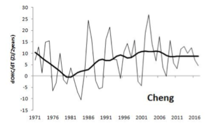
Fig.2: The dOHC/dt development with a 15 years Loess smooth
The result gives a very similar picture, indicating a near zero (or even a slightly falling) trend during 1999….2018 for the EEI.
What does this mean for the climate sensitivity?
Equilibrium/effective climate sensitivity (ECS) can be estimated as the (scaled) slope of the relationship between observed Global Mean Surface Temperature (GMST) and the excess of effective radiative forcing (ERF) over EEI, provided that the influence of natural climate system internal variability is small enough over the analysis period.
When there is an EEI standstill over a given period, then during this time the slope of the relationship between the observed GMST and the ERF reflects the climate sensitivity in equilibrium.
Sensitivity estimate for 1999…2018
The observed time span is very short for this purpose, only 20 years. This limits the toolbox available for doing calculations. In Lewis/Curry (2018) (LC18) the authors take changes between base and -final periods for both ERF and GMST data, see their section 4.
This avoids some pitfalls from the dilution problem of regression approaches which biases the slope estimations low. However, that method is only suitable with long enough time windows. Therefore I apply the regression method, including all annual data, in this case not using OLS (for Ordinary Least Square) regression but Deming regression. This method takes into account the uncertainties in variables from both datasets used, ERF and GMST, and should avoid the regression dilution problem.
The short time window will make optimizing the S/N ratio very crucial due to the fluctuating non-anthropogenic influences. Therefore I tried to reduce the “climate noise” in the GMST dataset- HadSST4 based Cowtan and Way (C&W) in this case.
I adjusted it for ENSO, solar and volcano influences, very similarly as was shown here. The “filter” was developed by Grant Foster aka “tamino”, released here.
The ERF data used are the same as used in L/C18, updated by the lead author to 2018.
Results
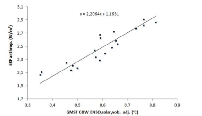
Fig.3: Deming Regression of the ERF on filtered GMST for 1999…2018 when the EEI was in a temporary standstill. All estimated natural forcing and ENSO variability was filtered out in the GMST, therefore the total anthropogenic ERF is used.
The trend slope reflects the observed climate feedback parameter λ (in W/m²/K).
The R² of the calculated trend is 0.88, which is a remarkably high value, when one takes the short time span involved into account.
The derived ECS best estimate (based on an ERF of 3.8 W/m² when doubling the CO2 content of the atmosphere) is:
3.8 W/m² / 2.21 W/m²/K =1.72 K
Conclusion
I calculated the climate sensitivity in a temporary standstill period (or slightly decreasing) as it was detected in the observations of the EEI during 1999 to 2018. The ECS value of 1.72K as the best estimate is in excellent agreement with the value found in LC18, 1.66K using the then current C&W GMST dataset (see Tab.3 of this paper).
The published ECS-values of the CMIP6 models have a mean above 4 K (see this recent paper) that is higher by a factor of 2.4 than observed here. This growing discrepancy between observed values of ECS reduces the credibility of the high model estimates.
K is the scale.
C is the unit.
1.72 K is 1.72 C above absolute zero aka -271.28 C
no it is not. 1.72°C is 1.72K above 0°C or 274.87K.
1.72C is an electrical unit (Coulomb).
@Nick Schroeder
Sure ?
I’m not 😀
K is both the scale and unit, so correct, but unnecessary. Everyone knows what was intended.
Just 2 more cents.
1°C is different from 1C°.
One is the unit measure — the size of one C degree — while the other is a temperature.
K, on the other hand does not use ° symbol. “1K” is ambiguous (context is usually clear): It could mean the size of a degree or a temperature 1C° above absolute zero.
It could also be the value of a resistor in an electronic circuit, but in this case we know that it is not.
Can we at least agree that a mil is 1/39370th (about) of a meter?
I’ve been seeing a lot of “metric” morons who think prefixes are measurements.
These are “delta” (change) values. The ECS estimate is 1.72K per doubling of atmospheric CO2. A delta of 1.72K per doubling of atmospheric CO2 is also a delta of 1.72 °C per doubling of atmospheric CO2.
0K = −273.15 °C
273.15K = 0 °C
Δ1.72K = Δ1.72 °C
You explained well, David, before I needed to.
It does worry me that anyone thought otherwise. !!
I doubt anyone thought otherwise. When some people cannot question the science they nitpick to try and decrease the legitimacy of the author – playing the man instead of the ball.
Thank heavens at least one person on here knows the relationship between kelvin and centigrade degrees.
“It is indeed surprising that the EEI not climbed during the last 19 years when taking into account the ongoing increase of forcing, arising mainly from rising greenhouse gas levels.”
Whooo hoo, a conclusion-based conclusion. Are we not beyond that ultra-sh!t science by now? I guess not.
How do you remove estimated natural forcing from GMST?
You fake it.
Or just pretend it doesn’t exist. 😉
With a spoon.
You forgot the essential Climate Science adjustments, which, when applied, bring Climate Sensitivity up to about 4 or 5…
https://youtu.be/DOUdQtubR6M
Dodgy G
You are on the right track! It is all about the uncertainty.
1.7 = 4.0 for very large values of 1.7.
large values of 1.7.
=======
Confess. You copied that from the IPCC latest report. Summary for Policy Makers.
What else are we to expect?
Solar activity has been declining since 2000.
http://www.vukcevic.co.uk/SSN-EEI.htm
Nice work!
Activity is intensity?
I wonder what the balance would be if the Arctic Ocean was iced over to an extent more like what we had in 180 or earlier.
MoD; Still having trouble getting my posts up
They have pills for that problem these days
Sorry. l think all this talk about climate sensitivity is also nonsense.
Click on my name to understand why I say that. It is all about Henry’ s Law….
What I would like to know is why NH SST is rising much faster than SH SST.
See
http://www.woodfortrees.org/plot/hadsst3gl/from:1964/plot/hadsst3nh/from:1964/plot/hadsst3sh/from:1964/plot/hadsst3gl/from:1964/trend
Because the ocean surfaces in the NH are more polluted than the SH. It’s out of date so it understates the problem, but this gives the gist of my argument:
https://seawifs.gsfc.nasa.gov/OCEAN_PLANET/HTML/peril_oil_pollution.html
My pleasure.
JF
I’ve said this over and over again. I’m in the process of writing it up at length. When finished I’ll send it out and then go off and do something else.
“This growing discrepancy between observed values of ECS reduces the credibility of the high model estimates.”
They have no real credibility component. They only have virtual credibility in the circle of junk science GCM climate modeling and its willful courtiers. No more credibility than claiming to see the Emperor’s New Clothes.
Excellent summation and analogy, Joel!
I am not sure I followed this article’s logic.
Are we assuming all natural warming has disappeared and so all current warming is the fault of extra CO2 primarily from fossil fuels? Or are we assuming that there is natural warming but all of it comes from nature adding CO2 into the air?
Or was natural warming somehow accounted for and I missed it?
So, if we accept that the Earth was already warming before CO2 levels were affected much by modern man, (I use 1960), then you should subtract that trend from whatever it is you are computing go get sensitivity.
1.72 degrees C still sounds high to me, I keep coming up with a number closer to 1 degree C when I run simple spreadsheets on past data. But at least your number is headed in the right direction (downward). (I estimate using raw land temperature measurements, include an estimate UHI, and remove warming I estimate is natural by looking at the warming trend before 1960 and assume that has not changed) In short, my complete guess is lower than your complete guess – but then I don’t publish my complete guess because I recognize its a complete guess. LOL
Getting clearer that the ECS range IS actually getting more accurate, but anything other than the climate-change industrial complex approved values are going to be hidden/ignored in any “official” literature (1.72K is not nearly scary enough). Still, this kind of legitimate research is one of the truly useful projects.
My personal frustration with most of this discussion is that we “talk up” one aspect or another, or another. And WOW, sometimes 2 or 3 interacting datasets and trendlines! Woot.
But aren’t there really more than 5, probably more than 8 or 10 “in the grand scheme of things climate” that need to be simultaneously synthesized into both a reflectively-accurate “pastcasting” model, and without tweaking an equally believable future model?
⋅-⋅-⋅ Just saying, ⋅-⋅-⋅
⋅-=≡ GoatGuy ✓ ≡=-⋅
See
http://www.woodfortrees.org/plot/hadsst3gl/from:1964/plot/hadsst3nh/from:1964/plot/hadsst3sh/from:1964/plot/hadsst3gl/from:1964/trend
I am hoping anybody who reads the comments here has maybe an idea as to why Nh SST is rising so much faster than Sh SST?
Henry Pool – Sorry I can’t give you an answer, but I can give you a suggestion: If the global climate is driven at least in part by the higher-latitude oceans of the Southern Hemisphere, then maybe you would get the effect you have observed. NB. Higher not highest.
The article above didn’t explicitly say that Northern Hemisphere sea surface temperatures are rising faster than those in the Southern Hemisphere.
But if that is indeed true, it may be due to the much larger land area in the temperate areas of the Northern Hemisphere than in the Southern Hemisphere. If there is a positive Earth Energy Imbalance, then air temperatures over both hemispheres (with seasonal variations filtered out) would be gradually warming. But over the Southern Hemisphere, dominated by ocean, any warming would tend to lead to increased evaporation, and the latent heat required for the additional evaporation would remove most of the temperature increase in the air, and remove heat from the ocean water.
In the temperate areas of the Northern Hemisphere, a substantial fraction of the area is dry land, where an increase in air temperatures (particularly in spring and summer) would not result in increased evaporation over land, but only an increase in the ground surface temperature. Warm air blowing off the coast from a continent could lead to a stronger thermal gradient between air and water, and there would be less surface area available for evaporation from the oceans. If there is an anticyclone over the coastal area, this effect can be tempered by the “sea breeze” during daylight hours, but weather fronts can cause warm air to be blown from the continent over the ocean for a few days at a time.
Here is something I noticed last month. I save daily screenshots from earthnullschool. One location is a sst save a bit north of Finland and between the two islands. On Dec 21st the location registered 30.7 C. That jumped to 31.9 C the next day, and on the 23rd the temp jumped to 34.8 C. How did that happen?
At the same time, earthnullschool had a weird change in ssta detail everywhere around the globe. I have daily screenshots for all of that. It doesn’t look right, and I have been looking at this every day for over 6 years now.
They recently changed the source of the SST data,
from: RTG-SST / NCEP /US National Weather Sevice
to: OSTIA / UK Met Office + GHRSST + CMEMS
Fine and dandy, now earthnullschool no longer correlates with either WeatherZone or Tropical Tidbits view of the ENSO regions, and also has differences elsewhere.. It shows a higher heat anomaly in the eastern zones of the ENSO than either of the 2 others. Someone is wrong.
why should they rise at the same rate? They are different in all sorts of ways.
Have a look at this
Maybe you realise the greater contact of the SH sea to the pole, in contrast to NH sea. So are more cold currents in the SH than in NH
Take a look at this, … https://goldminor.wordpress.com/2020/01/14/earthnullschool-puzzle/
Henry Pool,
The reason the NH SST is higher is that the SST measurement includes areas of sea ice. As the NH sea ice melts the temperature rises significantly in those areas because the sea ice acts as an insulator and prevents the ocean water from warming the air.
If you look closely the difference is only in the winter. In the summer the Arctic is above freezing which is about the same temperature as the ocean water. Hence, it doesn’t matter whether there is ice present.
I have a very simple comment about the energy imbalance.
According to my understanding this imbalance is the observed difference between the incoming solar radiation and the outgoing longwave radiation at the TOA over a longer period (several years). Incoming solar radiation is the difference between the solar insolation and the reflected SW radiation by the Earth.
This means that three measurements are needed for calculating the imbalance. Now two definitions are needed:
– Accuracy describes the difference between the measurement and the part’s actual value,
– Precision describes the variation you see when you measure the same part repeatedly with the same device.
Because it is a question of three different measurements, we have to know the accuracy of the measurements. Let us assume that the accuracies of these measurements are +/- 1 W/m^2. It means that an energy imbalance can be even +/- 3 W/m^2 and it is still just a measurement error. I suppose that the global radiation measurements are not better than +/- 1 W/m^2.
I think that it is impossible to find out any real result about the energy imbalance of the Earth based on the real measurement observations.
My question is how are we measuring the outgoing radiation? is it one, two, ten or thousands of satellites?
It would seem to me that the radiation leaving the atmosphere would be more uniform in distribution than the energy entering. This would make it very difficult to calculate what the number actually is, it would not just be a measurement, so by necessity it would be a model and how accurate or precise would that than be?
So nothing to worry about
Nothing at all to worry about. The transient climate response (TCR) is the immediate warming. This is generally about 2/3 of the ECS. A 1.72K ECS is only about a 1.16K TCR… 1.16K of warming at the time of the doubling. The remaining warming would occur over several hundred years.
I find it hilarious that we measure something in seconds (Joules/second) and describe its effect in decade.
There is no sensitivity to CO2.
There is some sensitivity to CO2, but it’s relatively insignificant.
How speculative us the ECS over the required several centuries?
I am hoping anybody who reads the comments here has maybe an idea as to why Nh SST is rising so much faster than Sh SST?
Hi Henry, perhaps these two reasons
more water in SH, it takes longer to warm up. The main reason is the strong Antarctic’s circumpolar current in the Southern ocean while both N.Atlantic and Pacific have only week links with cold Arctic waters.
https://en.wikipedia.org/wiki/Thermohaline_circulation#/media/File:Conveyor_belt.svg
Maybe because oceans move about. Maybe because the clean air acts raised insolation mainly in the NH.
Wonder what earthnull would have shown back in the 1960s/70s, … https://earth.nullschool.net/#current/chem/surface/level/overlay=so2smass/orthographic=-240.91,54.00,492/loc=-129.443,42.984
If the co2 that Is released from the ocean will raise temperature that will then provoke more rerelease of co2 which will then raise temperature etc, we immediately have a runaway process, unless there is another substance that puts a brake on it. So in principle co2 cannot raise the temperature. At least not as much as clouds can reduce it through albido. The alarmists claim that the co2 warming is amplified by water vapor. If that is the case we would have a runaway heating right away. Can anybody please tell me if there is a problem with my reasoning?
The surface of the ocean is fairly warm- it’s average surface temperature is about 17 C. And average land surface air temperature is about 10 C- which gives the average global air temperature of about 15 C.
But the ocean which is holding, CO2 is cold- the volume average temperature of the entire ocean is about 3.5 C. And the 3.5 C average temperature has not warm much over last 100 year and require increase in temperature of the ocean depths to release CO2- or an increase ocean surface temperature will not release CO2.
If had an increase of entire ocean by .5 C, one will thermal expansion which will be around 12″ of sea level rise. And over last century we had sea level rise of about 7″ and about 2″ of increase in sea level rise is thought to be due to the thermal expansion of the ocean.
If water amplifies CO2 then water would amplify water and there would be runaway warming in the absence of CO2. This is how you know the AGW hypothesis is wrong
I commented on this over at Judith’s, but will make a similar partial comment here.
This post is IMO very useful, albeit of limited statistical significance because of the relatively short data duration. It provides another triangulation on what ECS approximately ‘really is’
AR4 said 3; AR5 CMIP5 model mean is 3.2. 3ish
Lewis and Curry 2018 EbM method best estimate is about 1.67. Over at Judiths, DocMartin posted an estimate on 5/16/2013 using a different method to estimate 1.71. In 2014 Loehle used another method to publish an estimate of 1.7 in Ecological Modeling. In 2015 I used the then new Monckton Irreducibly Simple Equation paper to estimate about 1.7-1.75, in a complex critique of his paper at Climate Etc. (That post contains both a math critique and a derivation of the last two parameters of 5 needed by Monckton’s equation to estimate ECS (his other three parameters were uncontroversial IPCC that I plugged in). And now Franke Bosse has produced another independent estimate ~1.7.
No matter whether ‘really’ 1.6 or 1.8, the ECS zone is ~1.7, just over half of AR4 and AR5, and significantly under half of the reported AR6 value. And that is a BIG deal.
And… Don’t forget that TCR is what really matters. An ECS of 1.72K equates to a TCR of only about 1.16K. Assuming the doubling of pre-industrial CO2 occurs around the end of this century, the 1.5 °C “limit” won’t be breached.
This would imply (through careful goalpost mobility analysis), that the new tipping point leading to our extinction should be expected to be 1K, with this target being discovered before 2025, and announced by EurekAlert! as “worse than we thought”, or did I make a mistake somewhere?
“This would imply (through careful goalpost mobility analysis), that the new tipping point leading to our extinction should be expected to be 1K”
That’s exactly right! The Alarmists started out saying we could not afford to exceed 2C if we wanted to avoid a climate disaster, but then the estimates of the amount of warmth CO2 might add to the atmosphere kept going lower and lower and so the Alarmists decided that 2C wasn’t low enough to cause panic so they reduced the redline to 1.5C, and as you say, they will probably go lower as the estimates go lower. Goalpost mobility! 🙂
This Human-caused Climate change scam would actually be funny if it didn’t cost so much money, and didn’t drive so many people crazy. In reality, it is a horrible, deadly attack on human society.
The discrepancy lays bare the fake science at work in the climate models the IPCC uses. An agenda couldn’t be more obvious.
“This post is IMO very useful, albeit of limited statistical significance…”
It can’t be both of those things!
Pete, yes it can be, when you are just trying to triangulate an approximate answer—-especially, as here, when the precise answer not matter.
Rud, thanks for your kindly comments.
Given that the short duration of the dataset reduces it’s usefulness, can this help us design better data collection systems for the next 30 years of measurements.
and still the sun is blank
Hi Mm
There were about couple of the SC25 spots, the total January’s daily count to date is 82. If there were no more spots then the Jan’s count would be about 2.6 by the new revised method.
I don’t k ow the answer to this question, so enlightenment would be gratefully received.
Does it take more energy to raise the temperature of a given amount of water with dissolved CO2 than water without? Supplementary, is the answer the same for all gases ie O2 or Nitrogen.?
Firstly a given volume of water has 3000+ times more heat in it than an equal volume of air. I’m not sure about CO2. My own guess is both CO2 and air would have a small effect on water. Bottom line even with significant amount of dissolved air or CO2 the air over water will have a insignificant impact on the temperature of water.
The specific heat of seawater is less than pure water due to the presence of dissolved species, mainly salt. Both salt and CO2 have similar specific heat; about 25% of that of pure water. So dissolving CO2 into water reduces the specific heat of the combination compared with pure water. However it is only a very small reduction due to the limit on how much CO2 can be dissolved in the water.
There is a limit to how much CO2 can be dissolved into water. At typical ocean temperatures it is a very small proportion of the total mixture. Most of the CO2 is held as HCO3 negative ion so more CO2 results in an increase in pH and that counters further increase for given temperature, pressure and other species present.
There is a limit to how much CO2 can be dissolved into water. At typical ocean temperatures it is a very small proportion of the total mixture. Most of the CO2 is held as HCO3 negative ion so more CO2 results in an decrease in pH
I think the important point is warming air temperatures have a negligible impact on ocean temperatures. Therefore little impact on tropical storm formation eg hurricanes
Here’s a more realistic view of the energy imbalance.
Psun is the non reflected solar input (yellow), Pi is net solar input (blue), Po is total radiated by the planet (brown) and their difference is the flux in and out of the planet’s thermal mass, dE/dt (red). The equivalent radiant BB emissions of the surface corresponding to its temprature are also plotted. The first 3 plots represent the monthly averages over 3 decades of satellite data. These plots are all normalized and centered on their averages, so pay careful attention to the scales (avg+lim and avg-lim) which are different per item plotted.
First is the global data: No time constant, tau, can be calculated for the global response, as the output is out of phase with the input as a result of the asymmetries between hemispheres where the S has more p-p solar input, while the N has more p-p surface and planet emissions.
http://www.palisad.com/co2/plots/wbg/g/flux.png
Here is the data per hemisphere where time constants relative to surface change can be more easily inferred by the ratio of the peak to peak Pi and the peak to peak Psurf:
http://www.palisad.com/co2/plots/wbg/nh/flux.png
http://www.palisad.com/co2/plots/wbg/sh/flux.png
This one shows the individual months global data.
http://www.palisad.com/co2/flux/flux_g.png
And these are per hemisphere.
http://www.palisad.com/co2/flux/flux_nh.png
http://www.palisad.com/co2/flux/flux_sh.png
There does seem to be a small difference between W/m^2 in and W/m^2 out, however; the hemispheres do not get the same amount of Sun nor do they contribute equally to the total emissions and the amount of difference is within the margin of error. While Pi can be accurately obtained, Po requires a more complex calculation involving many terms, each with their own unique contributions to the uncertainty. The bottom line is that an average difference of zero is well within the margin of error.
Notice that a sinusoidal input (Pi) produces a sinusoidal surface output (Psurf) and a sinusoidal planet output (Po). This is the expected response of a first order LTI system, where the relevant differential equation is Pi = Po + dE/dt, where T is linear to E, Po is linear Psurf and Psurf is linear to T^4, where T is the surface temperature and Psurf are the equivalent BB emissions at that temperature.
The heat into the SH oceans during the Austral summer drive up water vapour about 90 degrees out of phase with the insolation due to the thermal lag of the oceans. As the atmospheric water vapour increases, the OLR increases. Simple, OLR and water vapour are highly positively correlated throughout the annual planetary warming and cooling cycle.
Every dip on the CERES graph correlates with a negative ENSO. Can’t help but wonder why the ENSO is not currently negative.
It seems to me that the idea that there is an ECS is fundamentally flawed. Climate is a complex, non-linear system. Trying to measure how such systems behave when one input changes by the change in one very crude number (a global average temperature) is pretty meaningless. This seems to arise because people equate temperature with energy, but the two are not the same. It also arises because people assume the climate is otherwise “stable” but complex non-linear systems are not stable, except at crude levels. By definition, such systems are composed of a large number of parts that are constantly interacting and thus constantly changing.
Phoenix44,
Linearity depends on the units of the metrics you’re quantifying relative to each other. If you’re quantifying the relationship between W/m^2 of any power flux and the T of any dependent matter in degrees (i.e. the planet), it’s very non linear where W/m^2 are proportional to T^4. If you’re quantifying the relationship between the power entering and leaving that matter, it’s very linear, even instantaneously relative to the bulk, where in the steady state, their accumulated sums are equal to each other on either side of a Gaussian surface enclosing the matter in direct equilibrium (the surface) with the incident power flux (the sun), independent of what’s between that matter (an atmosphere) and its environment (space). The average relationships between W/m^2 of BB surface emissions corresponding to its temperature and both W/m^2 of input and W/m^2 of output are very linear, maintaining a relatively constant steady state ratio between each pair of metrics. In general, when arbitrary metrics of a passive, causal system are expressed in units that are linearly related to each other, the metrics themselves are also linearly related to each other.
There are exceptions, for example, ferrites relative to magnetic fields, but nothing like that exists in the climate system. However; the only stuff in the atmosphere are things like GHG molecules, aerosols and the liquid and solid water in clouds., all of which in the steady state must be both absorbing and emitting the same W/m^2. There’s nothing intrinsically non linear about this. Calling the climate system non linear is a ploy designed to overlook and thus ignore the intrinsic linearity between metrics expressed in the same units. Once the linearity of the relationships between average W/m^2 of input, output and surface emissions is recognized, the entire range of the ECS presumed by the IPCC becomes impossible.
I posted some plots in an earlier comment (it’s in moderation because of too many links …) that shows how linear the relationships between metrics expressed in W/m^2 really are. The basic linear response is a time varying output proportional to a time varying input, with a proportionality constant and delay quantified by a time constant.
No it doesn’t. The only people surprised by this are those who believe it has any relevance to climate on Earth. The “greenhouse effect” is easily proven false by NASA’s own data that shows OLR rising as water vapour rises and OLR falling as water vapour falls – the exact opposite of the claimed “greenhouse effect”.
That would imply that the many heavy rains coming hitting many nations around the NH are a sign of a cooling trend. Many locations have experienced heavy rains or 100 year rains/snows in recent months. Here is today’s flood story, … https://watchers.news/2020/01/13/uae-smashes-24-year-old-rainfall-record-widespread-flooding-and-destruction-reported/
The day before was Pakistan, over the weekend Israel and Syria. Parts of Iran for the last 6 days. Extreme cold and heavy snow hit Afghanistan, killing at least 17 people…”. The list is growing.
Thank you. I also found the Bosse study interesting in more ways than one. Btw his estimate of 1.72 is close to the amazingly stable UAH temperature estimate of 1.8
Reported in this blog post
https://tambonthongchai.com/2020/01/09/agwmath/
I’m delighted to see lower estimates of ECS. On the other hand, I’m skeptical. The calculation of the planet’s energy balance requires that we know how much energy is radiated to space. Currently, that data is iffy.
The Europeans are launching a new satellite, the Far-infrared Outgoing Radiation Understanding and Monitoring (FORUM) project, sometime around 2025 or 2026.
Weather satellites accurately measure the outgoing LWIR in a few narrow bands, mostly in the transparent regions of the spectrum. It’s possible to infer the total LWIR from that data once it’s understood how the atmosphere passes W/m^2 from the surface to space through both clear skies cloudy skies. This is what I did to generate Po for the plots in a previous comment. Given that the incident energy and reflection are very accurately measured, the fact that the reconstructed Po’s global average is within a few W/m^2 of average Pi tells me that my calculation is relatively close.
Note that the seasonal imbalance per hemisphere varies between emitting up to 80 W/m^2 too much in the winter while up to 80 W/m^2 too little are emitted in the summer. When you subtract one big number from another big number and the difference is less than the uncertainty in the 2 large numbers, the net ‘imbalance’ is meaningless. In this case, we actually have 4 big numbers, 2 per hemisphere.
It’s also crucially important to recognize that the hemispheres respond independently to the Sun. While mathematically, the S hemisphere mostly ‘cancels’ the N hemisphere relative to the global averages, functionally they don’t cancel and are independent. They don’t quite cancel mathematically and the signature of the N hemisphere response is present in the global response.
I will be a whole lot happier when we have real data. Clouds are a real bear.
commieBob,
The reflectivity component is well measured in the satellite data, whether from clouds or the surface. The absorption component of clouds is definitely trickier, but the one thing the ISCCP data is good at is reporting cloud properties, including cloud top emission temperatures. Predicting those properties is definitely very hard, but once the properties are known, the analysis gets easier.
Clouds are broadband absorbers and radiators, while GHG’s are narrow band absorbers and radiators. In both cases, about half of what’s absorbed eventually ends up going to space while the remaining half is returned to the surface. Considering exactly 1/2 makes calculating and cross checking the absorption easier by balancing over multiples of years. Based on the results, it seems close enough.
Some good. full spectrum data will be very useful for fine tuning the understanding of how the atmosphere passes LWIR between the surface and space which will improve the usefulness of decades of narrow spectrum satellite data.
NH vs SH warming? Well look up videos of the work of Allan Savory and John D. Liu not to mention Anthony Watts and what he discovered with our Stevenson Screens. Where is most of the desertification and unnatural ground cover and I’ll even give Al Gore a mention in that regard-
https://www.theguardian.com/environment/2009/apr/28/black-carbon-emissions
Is that more relevant than their CO2 with any detectable anthropogenic warming? One thing I know with the really big picture is they have no correlation between the one true proxy for temperature in sea level movement and CO2 so they should be looking elsewhere for any possible dooming but they’re not. The Groupthink and hysteria is rather perplexing in that regard but science and the scientific method will prevail.
Speaking of deserts there’s one in the Pacific Ocean but then you all knew that because science is settled-
https://www.msn.com/en-au/news/techandscience/theres-a-desert-in-the-middle-of-the-pacific-and-we-now-know-what-lives-there/ar-BBYVh80
What! No nutrients from all that nasty human runoff on land and no warmening? Green Utopia.
@Julian Flood
Thanks for your comment!! I am finding your theory [that the warming of the oceans occurs due to contamination with oil/organics and general pollution] very interesting.
I have noticed that our ionic waste (especially phosphates, nitrates & sulfates) often stimulates algae growth and other primitive forms of live. I am sure this could also be a factor trapping heat in the oceans.
Is there perhaps a way we can prove the theory by actual testing?
J Flood..
Looked at your W.F.Trees link in more detail.
Cannot post links in here, but set the input parameters to 1850 instead of 1970.
You may be surprised to find that the situation you described with NH higher than SH also occurred in the period before 1900. It really does look like it is a cyclic behaviour as in the 1920 – 39 period it went into reverse..
I am sure (If we can trust the data), that something can be gleaned from the results.
I will leave it to other more specialised people to try and decode and produce any theories..
@Dave UK
Interesting. I am going it have a look at it. I wonder if it has to do with the GB cycle?
Click on my name.
It seems Dave UK is right. The rise between 1850 and 1880 was also much higher in the NH.
It must be the sun? Vuk?
Three things:
1. Estimates of ECS and TCR assume that all temperature changes are related to CO2 concentration. This allows hard-line skeptics to say “ECS is zero, recent warming is natural”. It also allows alarmists to say “there has to be (unspecified as to source) natural cooling of x, so ECS is really 1.7 + x”
2. Incoming is about 1349 w/m² and outgoing is about 1348 w/m². This makes measurement of EEI a classic case of “small difference between two large numbers”. Are they really measuring radiative fluxes with an accuracy of a small fraction of 1 w/m²? Authors citing the data don’t seem to be raising this question.
3. I keep speculating that the sw IR sensor must be detecting over a directional range of less than a half-space, otherwise it would pick up incoming solar when it crosses from night to day. Depending on the actual aperture angle, it is going to be more or less downward-looking. As such, interpreting the data must include theassumption that reflected sw comes from diffuse surfaces like clouds and snow, and that will make it omnidirectional.
But there will be a small amount of low-angle reflection that will come at the satellites sideways, and not be detected by downward-looking sensors. Low-angle reflection can come from calm seas and lakes and bare ice in Arctic regions when there is surface melting). Could the amount of this low-angle reflection be about 1 w/m²?
@Julian/ DaveUK
http://www.woodfortrees.org/plot/hadsst3gl/from:1850/plot/hadsst3nh/from:1850/plot/hadsst3sh/from:1850/plot/hadsst3gl/from:1850/trend
looking at SST from 1850,
actually shows less much less warming as well…
Is that really only 0.5K from 1850 till now?