Guest post by Pat Frank
Readers of Watts Up With That will know from Mark I that for six years I have been trying to publish a manuscript with the post title. Well, it has passed peer review and is now published at Frontiers in Earth Science: Atmospheric Science. The paper demonstrates that climate models have no predictive value.
Before going further, my deep thanks to Anthony Watts for giving a voice to independent thought. So many have sought to suppress it (freedom denialists?). His gift to us (and to America) is beyond calculation. And to Charles the moderator, my eternal gratitude for making it happen.
Onward: the paper is open access. It can be found here , where it can be downloaded; the Supporting Information (SI) is here (7.4 MB pdf).
I would like to publicly honor my manuscript editor Dr. Jing-Jia Luo, who displayed the courage of a scientist; a level of professional integrity found lacking among so many during my 6-year journey.
Dr. Luo chose four reviewers, three of whom were apparently not conflicted by investment in the AGW status-quo. They produced critically constructive reviews that helped improve the manuscript. To these reviewers I am very grateful. They provided the dispassionate professionalism and integrity that had been in very rare evidence within my prior submissions.
So, all honor to the editors and reviewers of Frontiers in Earth Science. They rose above the partisan and hewed the principled standards of science when so many did not, and do not.
A digression into the state of practice: Anyone wishing a deep dive can download the entire corpus of reviews and responses for all 13 prior submissions, here (60 MB zip file, Webroot scanned virus-free). Choose “free download” to avoid advertising blandishment.
Climate modelers produced about 25 of the prior 30 reviews. You’ll find repeated editorial rejections of the manuscript on the grounds of objectively incompetent negative reviews. I have written about that extraordinary reality at WUWT here and here. In 30 years of publishing in Chemistry, I never once experienced such a travesty of process. For example, this paper overturned a prediction from Molecular Dynamics and so had a very negative review, but the editor published anyway after our response.
In my prior experience, climate modelers:
· did not know to distinguish between accuracy and precision.
· did not understand that, for example, a ±15 C temperature uncertainty is not a physical temperature.
· did not realize that deriving a ±15 C uncertainty to condition a projected temperature does *not* mean the model itself is oscillating rapidly between icehouse and greenhouse climate predictions (an actual reviewer objection).
· confronted standard error propagation as a foreign concept.
· did not understand the significance or impact of a calibration experiment.
· did not understand the concept of instrumental or model resolution or that it has empirical limits
· did not understand physical error analysis at all.
· did not realize that ‘±n’ is not ‘+n.’
Some of these traits consistently show up in their papers. I’ve not seen one that deals properly with physical error, with model calibration, or with the impact of model physical error on the reliability of a projected climate.
More thorough-going analyses have been posted up at WUWT, here, here, and here, for example.
In climate model papers the typical uncertainty analyses are about precision, not about accuracy. They are appropriate to engineering models that reproduce observables within their calibration (tuning) bounds. They are not appropriate to physical models that predict future or unknown observables.
Climate modelers are evidently not trained in the scientific method. They are not trained to be scientists. They are not scientists. They are apparently not trained to evaluate the physical or predictive reliability of their own models. They do not manifest the attention to physical reasoning demanded by good scientific practice. In my prior experience they are actively hostile to any demonstration of that diagnosis.
In their hands, climate modeling has become a kind of subjectivist narrative, in the manner of the critical theory pseudo-scholarship that has so disfigured the academic Humanities and Sociology Departments, and that has actively promoted so much social strife. Call it Critical Global Warming Theory. Subjectivist narratives assume what should be proved (CO₂ emissions equate directly to sensible heat), their assumptions have the weight of evidence (CO₂ and temperature, see?), and every study is confirmatory (it’s worse than we thought).
Subjectivist narratives and academic critical theories are prejudicial constructs. They are in opposition to science and reason. Over the last 31 years, climate modeling has attained that state, with its descent into unquestioned assumptions and circular self-confirmations.
A summary of results: The paper shows that advanced climate models project air temperature merely as a linear extrapolation of greenhouse gas (GHG) forcing. That fact is multiply demonstrated, with the bulk of the demonstrations in the SI. A simple equation, linear in forcing, successfully emulates the air temperature projections of virtually any climate model. Willis Eschenbach also discovered that independently, awhile back.
After showing its efficacy in emulating GCM air temperature projections, the linear equation is used to propagate the root-mean-square annual average long-wave cloud forcing systematic error of climate models, through their air temperature projections.
The uncertainty in projected temperature is ±1.8 C after 1 year for a 0.6 C projection anomaly and ±18 C after 100 years for a 3.7 C projection anomaly. The predictive content in the projections is zero.
In short, climate models cannot predict future global air temperatures; not for one year and not for 100 years. Climate model air temperature projections are physically meaningless. They say nothing at all about the impact of CO₂ emissions, if any, on global air temperatures.
Here’s an example of how that plays out.

Panel a: blue points, GISS model E2-H-p1 RCP8.5 global air temperature projection anomalies. Red line, the linear emulation. Panel b: the same except with a green envelope showing the physical uncertainty bounds in the GISS projection due to the ±4 Wm⁻² annual average model long wave cloud forcing error. The uncertainty bounds were calculated starting at 2006.
Were the uncertainty to be calculated from the first projection year, 1850, (not shown in the Figure), the uncertainty bounds would be very much wider, even though the known 20th century temperatures are well reproduced. The reason is that the underlying physics within the model is not correct. Therefore, there’s no physical information about the climate in the projected 20th century temperatures, even though they are statistically close to observations (due to model tuning).
Physical uncertainty bounds represent the state of physical knowledge, not of statistical conformance. The projection is physically meaningless.
The uncertainty due to annual average model long wave cloud forcing error alone (±4 Wm⁻²) is about ±114 times larger than the annual average increase in CO₂ forcing (about 0.035 Wm⁻²). A complete inventory of model error would produce enormously greater uncertainty. Climate models are completely unable to resolve the effects of the small forcing perturbation from GHG emissions.
The unavoidable conclusion is that whatever impact CO₂ emissions may have on the climate cannot have been detected in the past and cannot be detected now.
It seems Exxon didn’t know, after all. Exxon couldn’t have known. Nor could anyone else.
Every single model air temperature projection since 1988 (and before) is physically meaningless. Every single detection-and-attribution study since then is physically meaningless. When it comes to CO₂ emissions and climate, no one knows what they’ve been talking about: not the IPCC, not Al Gore (we knew that), not even the most prominent of climate modelers, and certainly no political poser.
There is no valid physical theory of climate able to predict what CO₂ emissions will do to the climate, if anything. That theory does not yet exist.
The Stefan-Boltzmann equation is not a valid theory of climate, although people who should know better evidently think otherwise including the NAS and every US scientific society. Their behavior in this is the most amazing abandonment of critical thinking in the history of science.
Absent any physically valid causal deduction, and noting that the climate has multiple rapid response channels to changes in energy flux, and noting further that the climate is exhibiting nothing untoward, one is left with no bearing at all on how much warming, if any, additional CO₂ has produced or will produce.
From the perspective of physical science, it is very reasonable to conclude that any effect of CO₂ emissions is beyond present resolution, and even reasonable to suppose that any possible effect may be so small as to be undetectable within natural variation. Nothing among the present climate observables is in any way unusual.
The analysis upsets the entire IPCC applecart. It eviscerates the EPA’s endangerment finding, and removes climate alarm from the US 2020 election. There is no evidence whatever that CO₂ emissions have increased, are increasing, will increase, or even can increase, global average surface air temperature.
The analysis is straight-forward. It could have been done, and should have been done, 30 years ago. But was not.
All the dark significance attached to whatever is the Greenland ice-melt, or to glaciers retreating from their LIA high-stand, or to changes in Arctic winter ice, or to Bangladeshi deltaic floods, or to Kiribati, or to polar bears, is removed. None of it can be rationally or physically blamed on humans or on CO₂ emissions.
Although I am quite sure this study is definitive, those invested in the reigning consensus of alarm will almost certainly not stand down. The debate is unlikely to stop here.
Raising the eyes, finally, to regard the extended damage: I’d like to finish by turning to the ethical consequence of the global warming frenzy. After some study, one discovers that climate models cannot model the climate. This fact was made clear all the way back in 2001, with the publication of W. Soon, S. Baliunas, S. B. Idso, K. Y. Kondratyev, and E. S. Posmentier Modeling climatic effects of anthropogenic carbon dioxide emissions: unknowns and uncertainties. Climate Res. 18(3), 259-275, available here. The paper remains relevant.
In a well-functioning scientific environment, that paper would have put an end to the alarm about CO₂ emissions. But it didn’t.
Instead the paper was disparaged and then nearly universally ignored (Reading it in 2003 is what set me off. It was immediately obvious that climate modelers could not possibly know what they claimed to know). There will likely be attempts to do the same to my paper: derision followed by burial.
But we now know this for a certainty: all the frenzy about CO₂ and climate was for nothing.
All the anguished adults; all the despairing young people; all the grammar school children frightened to tears and recriminations by lessons about coming doom, and death, and destruction; all the social strife and dislocation. All the blaming, all the character assassinations, all the damaged careers, all the excess winter fuel-poverty deaths, all the men, women, and children continuing to live with indoor smoke, all the enormous sums diverted, all the blighted landscapes, all the chopped and burned birds and the disrupted bats, all the huge monies transferred from the middle class to rich subsidy-farmers.
All for nothing.
There’s plenty of blame to go around, but the betrayal of science garners the most. Those offenses would not have happened had not every single scientific society neglected its duty to diligence.
From the American Physical Society right through to the American Meteorological Association, they all abandoned their professional integrity, and with it their responsibility to defend and practice hard-minded science. Willful neglect? Who knows. Betrayal of science? Absolutely for sure.
Had the American Physical Society been as critical of claims about CO₂ and climate as they were of claims about palladium, deuterium, and cold fusion, none of this would have happened. But they were not.
The institutional betrayal could not be worse; worse than Lysenkoism because there was no Stalin to hold a gun to their heads. They all volunteered.
These outrages: the deaths, the injuries, the anguish, the strife, the malused resources, the ecological offenses, were in their hands to prevent and so are on their heads for account.
In my opinion, the management of every single US scientific society should resign in disgrace. Every single one of them. Starting with Marcia McNutt at the National Academy.
The IPCC should be defunded and shuttered forever.
And the EPA? Who exactly is it that should have rigorously engaged, but did not? In light of apparently studied incompetence at the center, shouldn’t all authority be returned to the states, where it belongs?
And, in a smaller but nevertheless real tragedy, who’s going to tell the so cynically abused Greta? My imagination shies away from that picture.
An Addendum to complete the diagnosis: It’s not just climate models.
Those who compile the global air temperature record do not even know to account for the resolution limits of the historical instruments, see here or here.
They have utterly ignored the systematic measurement error that riddles the air temperature record and renders it unfit for concluding anything about the historical climate, here, here and here.
These problems are in addition to bad siting and UHI effects.
The proxy paleo-temperature reconstructions, the third leg of alarmism, have no distinct relationship at all to physical temperature, here and here.
The whole AGW claim is built upon climate models that do not model the climate, upon climatologically useless air temperature measurements, and upon proxy paleo-temperature reconstructions that are not known to reconstruct temperature.
It all lives on false precision; a state of affairs fully described here, peer-reviewed and all.
Climate alarmism is artful pseudo-science all the way down; made to look like science, but which is not.
Pseudo-science not called out by any of the science organizations whose sole reason for existence is the integrity of science.
Wow! What a blockbuster of an article, Anthony. Knowledgeable people in the scientific and political communities need to read this article and the accompanying paper and SI and take this to heart. Especially the Republican Party. But of course, we know what that apocalyptic types will do. We must not allow that, especially in any attempt by the Trump administration to overturn the endangerment finding made by the previous (incompetent) administration.
Politicians, are mostly too thick, to understand it. That applies to any politician, any party, any country.
Politicians are following the money, as they always have done, that is, money for their own pockets
And the politicians (e.g. Trudeau, Gore) continue to fly a lot, continue to drive around in big SUVs, and continue to live in multiple, very large houses.
Often very close to those rising oceans……
Adam Gallon
100% correct, and the very reason why the climate alarmists stole a march on sceptics. They framed their argument politically, and everyone, irrespective of education, has the right to a political opinion. Sceptics chose the scientific route, and less that 10% of the world is scientifically educated.
When it comes time to vote, guess who gets the most, and the cheapest votes for their $/£?
And , so it seems , are the scientists “ mostly too thick “ !
Not too thick, only unsceptical. The more intelligent you are, the more you can utilise your intelligence to justify your need to believe something, and the more prone you will be to confirmation bias.
Cherry picking evidence that suits you and finding justifications to hand wave away that which doesn’t requires a good brain, but good brains are still at the mercy of their owners’ emotional defences, including pride, self interest, misplaced fear and stubbornness.
100 percent spot on. This is done in all areas of our society. Government, non government, business, media. People wordsmithing their agendas, justifying their actions. Corruption years ago was someone taking money under the table. These days it is taken over the table, people are just smarter in justifying their course of action. Sadly most of them believe their own rheteric.
Someone needs to get this Paper to trump…..
Have HIM go public with it….
And have him ask for rebuttal from the Climate Science world….. Since the clown media exacts their *freedom denialist* on him whenever they can…..
Don’t sit on this…….
Trump wouldn’t read it. He’d ask for the short version in 25 words or less.
The CACA crock is built upon climate models that don’t model climate, climatologically useless air temperature measurements, and proxy paleo-temperature reconstructions which don’t reconstruct temperature.
Edited down to 25 words.
Because error propagation.
@DanM: No, please please please don’t give it to Trump. His credibility is low — and falls further with every tweet. Trump’s daily dribble of dubious pronouncements is easily dismissed as ignorant, self-serving prattle.
We “deniers” need to stay focused on science vs. non-science, as the article’s author suggests. “Climate science” presents a non-falsifiable theory as inevitable outcome — as Richard Feynman once said, that is not science.
If we are to convince the “more educated” segment of society of the perniciousness of “climate science”, we must disentangle the science from the politics. The two are antithetical: The former is, very generally speaking, about parsing signal from noise; the latter is, very generally speaking, the exact opposite.
The “more educated” don’t get that yet, don’t get that their religious belief in CO2-induced End Times is based on corrupted scriptures. When they do, enlightenment will follow.
Richie, the skeptic community has been riven with dislike or distrust for too long. The spat between Anthony Watts and Tony Heller is a good example.
You may dislike Trump’s tweeting, but he is uniquely willing and able to take climastrology head on, and his tweets probably reach a group of people that your preferred approach never would.
If Trump picks this up and tweets it around, good for him, good for everyone. If you want to engage your community in a scientific debate, good for you.
There are plenty of alarmists out there pushing out nonsense, we don’t need to criticize each other for doing what we can, where we can, to push it back.
Richie, Trump is on only one in 30 years in politics to call BS on these climate terrorists. The only one to call BS on China trade practices. The only one willing to rescind a deal to give nukes to Iran. The only one to even mention the USA cannot just have everyone in the world move here. The only one to suggest NATO pay their own way. You need to listen to people that did not spout ‘Russian collusion” for 2+ years knowing it was a bald faced lie. You better get on board, as this guy is the ONLY one with credibility.
Trump will not read this paper and nor should he , he is not a scientist and has never pretended to be ! Contrary to popular belief I am sure, Trump nor all Ex presidents make ALL decisions such as this on subjects . Not one single person has the amount of knowledge or education required to “Run” a country . Trump rely’s on his advisers I am sure which is the right thing to do.
Actually, as grad of a good B-school, Trump must have taken statistics courses. He could read and understand, or at least get the gist of this paper, but his attention span is short and digesting the whole thing would be a waste of time for any president.
The abstract and conclusions, with a graph or two, in his daily summary would be the most for which we could or should hope.
Politicians don’t WANT to understand it (except Trump) AGW is a HUGE gravy train for them…
Not sure if I completely agree, Adam.
I agree that there are many who are too thick to understand, but there are also many who don’t want to understand and others that don’t have time to understand.
The don’t want to understand people don’t care. They are either already hard core Warm Cult or have been informed by their spin merchants that Climate Change is what their voters want. These are either ‘Science is Settled… and if it isn’t, then it should be’ or would support the reintroduction of blood sports if their internal polling said it would win them another term.
Then there are the ones who don’t have time to care. Politicians are busy people. All that sunshine isn’t going to get blown up people’s…. ummm… egos by itself you know. They don’t have time to sit down and read reports, they have Important Meetings to attend. Hence they surround themselves with staffers who – nominally – do all the reading for them and feed them the 10 word summary. Now that all sounds fine and dandy, and Your Country May Vary, but here in Oz most staffers are the 24 year olds who have successfully backstabbed and grovelled their way through the ‘Young’ branch of their party and the associated faction politics. Since very few of these people have anything remotely resembling a STEM background they are for all extents and purposes, masculine bovine mammaries.
Like they say, Sausages and Laws. 🙁
Great article.
In layman’s terms:
If the climate modelers were financial advisors the world would be living under one gigantic bridge.
If climate modelers were engineers, there wouldn’t be any bridges to live under.
Climate modelling is Cargo Cult Science!
Was it Freeman Dyson or Richard Feynman who stated this years ago?
Climate models are not real models.
Real models make right predictions.
Climate models make wrong predictions.
The so called “climate models”, and government bureaucrat “scientists” who programmed them, are merely props for the faith based claim that a climate crisis is in progress.
If people who joined conventional religions believed that, they would point to a bible as “proof”.
In the unconventional “religion” of climate change, their “bible” is the IPCC report, and their “priests” are government bureaucrat and university “scientists”.
Scientists and computer models are used as props, to support an “appeal to authority” about a “coming” climate crisis, coming for over 30 years, that never shows up !
In the conventional religions, the non-scientist “priests” and their bibles say: ‘You must do as we say, or you will go to hell’.
In the climate change “religion”, the scientist “priests” say: ‘You must do as we say, or the Earth will turn into hell for your children’.
” … the whole aim of practical politics is to keep the populace alarmed (and hence clamorous to be led to safety) by menacing it with an endless series of hobgoblins, most of them imaginary.”
— From H. L. Mencken’s In Defense of Women (1918).
.
.
My climate science blog:
http://www.elOnionBloggle.Blogspot.com
.
.
Concerning the Green New Deal:
“Politics is the art
of looking for trouble,
finding it everywhere,
diagnosing it incorrectly,
and applying the wrong remedies.”
Groucho Marx
It was Feynman. A commencement speech in the 70’s.
[excerpt from this excellent article]
“In their hands, climate modeling has become a kind of subjectivist narrative, in the manner of the critical theory pseudo-scholarship that has so disfigured the academic Humanities and Sociology Departments, and that has actively promoted so much social strife. Call it Critical Global Warming Theory. Subjectivist narratives assume what should be proved (CO₂ emissions equate directly to sensible heat), their assumptions have the weight of evidence (CO₂ and temperature, see?), and every study is confirmatory (it’s worse than we thought).
Subjectivist narratives and academic critical theories are prejudicial constructs. They are in opposition to science and reason. Over the last 31 years, climate modeling has attained that state, with its descent into unquestioned assumptions and circular self-confirmations.”
…
Raising the eyes, finally, to regard the extended damage: I’d like to finish by turning to the ethical consequence of the global warming frenzy. After some study, one discovers that climate models cannot model the climate. This fact was made clear all the way back in 2001, with the publication of W. Soon, S. Baliunas, S. B. Idso, K. Y. Kondratyev, and E. S. Posmentier Modeling climatic effects of anthropogenic carbon dioxide emissions: unknowns and uncertainties. Climate Res. 18(3), 259-275, available here. The paper remains relevant.
In a well-functioning scientific environment, that paper would have put an end to the alarm about CO₂ emissions. But it didn’t.
Instead the paper was disparaged and then nearly universally ignored (Reading it in 2003 is what set me off. It was immediately obvious that climate modelers could not possibly know what they claimed to know). There will likely be attempts to do the same to my paper: derision followed by burial.
But we now know this for a certainty: all the frenzy about CO₂ and climate was for nothing.
[end of excerpt]
So the false narrative of global warming alarmism has once again been exposed, even though this paper was REPRESSED for SIX YEARS!
It is absolutely clear, based on the evidence , that global warming and climate change alarmism was not only false, but fraudulent. Its senior proponents have cost society tens of trillions of dollars and many millions of lives – an entire global population has been traumatized by global warming alarmism, the greatest scientific fraud in history – these are crimes against humanity and their proponents belong in jail – for life!
Oh yes indeed. But who will do it?
Too many people are making too much money off of this ridiculous hoax. Too many politicians are acquiring too much power off of this insanity. The media spin their narrative continually because it plays into the leftist desire to smash capitalism.
We need somebody to break this thing once and for all. Trump has tried but he is so controversial in so many ways that the message is lost. So we will all just continue in our own little way trying to change the opinion of those close to us and hope that our own prophet will appear and throw the money lenders out of the temple of pseudo-science once and for all.
Is jail for life sufficient punishment for the theft of trillions in treasure and loss of life for tens of millions?
Pat’s math nonsense has been completely dismantled here:
https://patricktbrown.org/2017/01/25/do-propagation-of-error-calculations-invalidate-climate-model-projections-of-global-warming/
here:
https://andthentheresphysics.wordpress.com/2017/01/26/guest-post-do-propagation-of-error-calculations-invalidate-climate-model-projections/
and years ago here:
https://tamino.wordpress.com/2011/06/02/frankly-not/
…and by Nick Stokes here:
https://moyhu.blogspot.com/2019/09/another-round-of-pat-franks-propagation.html
and two years ago here:
https://moyhu.blogspot.com/2017/11/pat-frank-and-error-propagation-in-gcms.html
Unlike other zombie myth let us hope this one is finally laid to rest.
Hahahaha — tamino. Fortunately haven’t heard anything about that abomination for yrs….
Calling tamino names is not a scientific argument. We are claiming to be scientists. The standards that we impose upon ourselves must be rigorous.
Where is an analysis of the tamino paper that refutes tamino?
Apparently you didn’t bother to read Pat Frank’s responses.
It’s not surprising that a young computer gamer would object to Pat’s work. Young Dr. Brown would need to find a new career should Pat’s conclusions be confirmed.
There are 5 references put forward to refute Mr. Frank’s paper.
Calling people names is not a scientific argument.
You refer to Mr. Frank’s responses. Where are the references to his responses that allow a review of the arguments? Who are the people with sufficient credibility who stand behind Mr. Frank’s work and refute the arguments (pseudo arguments) put forth in these five references.
Lord Moncton has made a different argument that claims to demolish the alarmists. But the alarmists have put forward a criticism of Moncton that I have not seen addressed.
Rigorous argument is the hallmark of science. There is no shortcut.
No name calling. GIGO GCMs are science-free games. They are worse than worthless wastes of taxpayer dollars, except to show how deeply unphysical is the CACA scam.
Patrick Brown’s arguments did not withstand the test of debate, carried out beneath his video.
ATTP thinks (+/-) means constant offset. And Tamino ran away from the debate — which was about a different analysis anyway.
Nick’s moyhu posts are just safe-space reiterations of the arguments he failed to establish in open debate.
Skeptic t-shirt.
https://www.amazon.com/dp/B07XNNBBXZ
It’s brilliant, and the list looks pretty complete. 🙂
Missing at least one relevant point:
Uncertainty Propagation
I’ll have my wife add it on there after mine arrives. She’s good at that sort of thing and has produced a number of fun items for me to wear.
I never, ever buy t-shirts. I just bought this one. I could not resist. Thanks for the link.
How do you see the back? – there is no simple link !!!
Click on the small image of the back, then hover your mouse/cursor over the resultant view to see a magnified view.
OK, thanks for that ! I could’t find the image of the back of the Shirt…
It was way over to the left side on my screen, and couldn’t seem to locate it until I knew what to look for,
The list is pretty damn complete, thx !
JPP
I have been waiting for years hoping that someone would come up with an A+B proof that definitively buries the non-scientific proceedings of the “climate religion”. Pat Frank’s publication hits that nail with a beautiful hammer! Every student writing a report about a practical physics experiment has to calculate the error margins. That these so-called scientists (some are even at ETH Zurich) don’t even seem to understand what an error margin means was a real shock to me. Just recently I’ve been reading something about the UN urging for haste and mentioning that scientific arguments are not relevant anymore and should be ignored… Do you see something coming?
“…for giving a voice to independent thought.”
Although it’s been a struggle for some of us.
Add to the list of what people don’t know.
Most people don’t understand that at this distance from the sun objects get hot (394 K) not cold (- 430 F).
The atmosphere/0.3 albedo cools the earth compared to no atmosphere.
And because of a contiguous participating media, i.e. atmospheric molecules, ideal BB LWIR upwelling from the surface/oceans is not possible.
396 W/m^2 upwelling is not possible.
333 W/m^2 downwelling/”back” LWIR 100% perpetual loop does not exist.
RGHE theory goes into the rubbish bin of previous failed consensual theories.
Nick, you’ve got it wrong, it’s not a 333 feedback loop…. 396 – 333 = 63 watts per sq. M radiated from the ground to the sky on average. At the basic physics of it all, the negative term in the Stephan-Boltzmann two surfaces equation, which is referred to as “back radiation”, 333 watts in this case, is how much the energy content of the wave function of the hotter body is negated by a cooler body’s wave function. But only high level physicists think of it in those terms. Most just use the back radiation concept. So do climatologists. Engineers prefer to just use SB to calculate heat transfer from hot to cold directly, to be sure they don’t inadvertently get dreaded temperature crosses in their heat exchangers.
DMac
The 396 W/m^2 is a theoretical “what if” calculation for the ideal LWIR from a surface at 16 C, 289 K. It does not, in actual fact, exist.
The only way a surface radiates BB is into an vacuum where there are no other heat transfer processes occurring.
As demonstrated in the classical fashion, by actual experiment:
https://principia-scientific.org/debunking-the-greenhouse-gas-theory-with-a-boiling-water-pot/
No 396, no 333, no RGHE, no GHG warming.
“…how much the energy content of the wave function of the hotter body is negated by a cooler body’s wave function…”
Classical handwavium nonsense. If a cold body “negated” a hot body there would be refrigerators without power cords. I don’t know of any. You?
I think you both have it wrong. Two objects near each other send radiation back and forth continuously and the outgoing flux can be calculated using the temperature and albedo of each. The fact that an IR Thermometer works at all proves this to be true.
In the case of the Earth’s surface and a “half-silvered” atmosphere, there is a continuous escaping to space of some of the radiation from the surface (directly) and from the atmosphere (directly and indirectly) according to the GHG concentration.
I am weary of arguments that there is no “circuit” between the atmosphere and the surface. Of course there is – there is a thermal energy “circuit” between all objects that have line-of-sight of each other, including between me and the Sun. There is nothing mysterious about this. That is how radiation works.
A simple demonstration of this is to build a fire using one stick. Observe it. Make a sustainable fire as small as possible. Now split the stick in two and make another fire, placing the two sticks in parallel about 10 mm apart. The fire can be smaller than the previous one because the thermal radiation back and forth between the two is conserved. There is no net energy gain doing this for either stick, but there is net benefit (if the object is to make the smallest possible fire).
Radiation continues regardless of whether there is anything “on the receiving end” and always will.
“Two objects near each other send radiation back and forth continuously and the outgoing flux can be calculated using the temperature and albedo of each. The fact that an IR Thermometer works at all proves this to be true. ”
Is this what you have in mind: Q = sigma * A * (T1^4 – T2^4)
Where are the other 5 terms? 2 Qs, 2 epsilon, second area?
This is not “net” energy, it’s the work required to maintain the different temperatures.
Nonsense.
Two objects one hot and one cold: energy flows (heat) from the hot to the cold (EXCLUSIVELY) until they come to equilibrium. The only way to reverse this energy flow is by adding work in the form of a refrigeration cycle.
IR instruments are designed, fabricated and applied based on temperature sensing elements. Power flux is inferred based on an assumed emissivity.
Assuming 1.0 for the earth’s surface or much of molecular anything else is just flat wrong.
The Instruments & Measurements
But wait, you say, upwelling LWIR power flux is actually measured.
Well, no it’s not.
IR instruments, e.g. pyrheliometers, radiometers, etc. don’t directly measure power flux. They measure a relative temperature compared to heated/chilled/calibration/reference thermistors or thermopiles and INFER a power flux using that comparative temperature and ASSUMING an emissivity of 1.0. The Apogee instrument instruction book actually warns the owner/operator about this potential error noting that ground/surface emissivity can be less than 1.0.
That this warning went unheeded explains why SURFRAD upwelling LWIR with an assumed and uncorrected emissivity of 1.0 measures TWICE as much upwelling LWIR as incoming ISR, a rather egregious breach of energy conservation.
This also explains why USCRN data shows that the IR (SUR_TEMP) parallels the 1.5 m air temperature, (T_HR_AVG) and not the actual ground (SOIL_TEMP_5). The actual ground is warmer than the air temperature with few exceptions, contradicting the RGHE notion that the air warms the ground.
Sun warms the surface, surface warms the air, energy moves from surface to ToA according to Q = U A dT, same as the insulated walls of a house.
Nonsense.
All objects radiate, unless they are at absolute zero.
Net energy flows from the hot object to the cold object, but energy IS flowing in both directions.
This is a reply to your claim that “Two objects one hot and one cold: energy flows (heat) from the hot to the cold (EXCLUSIVELY) until they come to equilibrium.” Wrong. Energy flows in both directions (unless one happened to be at absolute zero); however, the energy flowing from the hotter object to the colder one is greater than the energy flow in the opposite direction. The result is that the NET flow is unidirectional until equilibrium. But flow =/= net flow.
You are absolutely correct CinW. Very close to the Earth’s surface a downward facing calculation using MODTRAN will produce the Stefan-Boltzmann with an emissivity of 0.97 just about exactly. The typical earth materials have emissivities averaging to about 0.97.
As one rises away from the Earth’s surface the calculated effective emissivity of the downward view will decline, eventually to a value of 0.63 or so, because of the intervening IR active gasses.
Claiming the SB law applies only to a cavity in vacuum is an utterly immaterial argument. The lack of a cavity is why emissivity is less than one for surfaces in vacuum.
I think you mean each of the 2 separated fires is a bit smaller than the original single fire…view factor considerations…but I’m thinking draft is an important factor for sticks 10 mm apart versus 0 mm…
Kevin kilty – September 7, 2019 at 6:50 pm
Utterly silly claim, ….. with no basis in fact.
The atmosphere is constantly moving across the surface of the Earth in weather patterns so it is unlikely that they will ever reach equilibrium unless a weather pattern becomes stuck and the surface is given time to reach equilibrium with the atmosphere. The surface temperature is heated by solar radiation but cools or heats up with thermal interaction with the atmosphere close to it. My model of the thermal Earth does not have any back radiation there is local thermal equilibrium between the surface and overlying atmosphere if the atmosphere remains static to give time for equilibrium to be reached.
Donald P, ….. I criticized Kevin kilty simply because the ppm density of Kevin’s stated “IR active gasses” is pretty much constantly changing, with H2O vapor being the dominant one. Also, the IR being radiated from the surface is not polarized, meaning, ……. the higher the elevation from the emitting surface, ….. the more diffused or spread out the IR radiation is. Just like the visible light from a lightbulb decreases in intensity (brightness) the farther away the viewer is.
Samuel C Cogar,
Before launching into someone, you ought to know what you are talking about. Run some models using the U of Chicago wrapper for MODTRAN and see what you get looking down close to the surface and again high in the atmosphere. I have run hundreds of MODTRAN models and they are very educational. By the way, MODTRAN is among the most reliable codes of any sort around (Tech. Cred. 9), so do not hide behind “its just a model”.
I have no idea why you do not understand the impact of IR active gasses in an atmosphere. The ramifications involve the sensors and controls in millions of boilers, furnaces, power plants, etc. Every day, all day long.
Nick, busses could drive through the holes in your experiment. You can’t disprove the negative term Thot^4-Tcold^4 in the SB equation with a boiling kettle. Because the instrumentation on many fired heaters and industrial furnaces confirm it every hour, every day, worldwide. I’ve designed some if them. SB is right, so there is a RGHE resulting from CO2 and H2O in the atmosphere. I know H2O and CO2 absorb and emit CO2 from many years of calculating it and reading instruments that confirm it. End of story.
>>>>>>MarkW
September 7, 2019 at 5:21 pm
”Nonsense.
All objects radiate, unless they are at absolute zero.
Net energy flows from the hot object to the cold object, but energy IS flowing in both directions.”<<<<<<
No reply function under your post so I put this here….please forgive..
As a non-scientist, I have trouble visualizing this. How can an object lose (emit) and gain (absorb) energy at the same time? What is the mechanism? (in simple terms)
Mike
How do things lose and gain energy [not heat] at the same time?
Consider two flashlights (torches in the UK) pointing at each other. The light from each shines out from the bulb and is, in part, received by the other. Now, suppose the batteries in one start to fade and the emission of light decreases. Will this affect the amount of light emerging from the other one? Not at all. Nothing about one light affects what the other does. They both shine as they are able, or not if they are turned off.
Nick S above is thinking about conduction of heat, not radiation of energy. Different rules apply for that. There are three modes of energy transfer: conduction, convection and radiation. People with no high school science education frequently confuse conduction and radiation lumping both into “transfer”.
Light is not conducted through the air from one flashlight to the other – it is radiated, and this would happen even if there was no air at all.
Now consider that the original IMAX projector had a 25 kilowatt short arc Xenon bulb in it which produced enough light to brightly illuminate that hundred foot wide screen. Point one at a flashlight. Is the flashlight’s radiance in any way “countered” or “dimmed” or “enhanced”? No not at all. They are independent, disconnected systems with a gap between that can only be bridged by the radiation of photons.
Infra-red radiations is a form of light, light with a wavelength below what we can perceive. Some insects can see IR, some snakes, not us. Some can see UV. We can’t see that either. Not being able to see it doesn’t mean it is not flowing like the visible photons from a flashlight. IR camera can see the IR radiation. The temperature is converted to colour scale for convenience. Basically it is a size-for-size wavelength conversion device.
It happens that all material in the universe is capable of emitting photons, but not nearly equally., however. Non-radiative gases are so-termed because they don’t emit (much) IR, but they will emit something if heated high enough. That doesn’t happen in the atmosphere.
It isn’t quite true that all objects will radiate energy down to absolute zero. That only applies to black objects or gases with absorption bands in the IR. We are only talking about IR radiation when we discuss the climate.
Something very interesting and rather counter-intuitive is that an object such as a piece of steel will have a certain emissivity, say 0.85. (Water is almost absolutely black in IR, BTW.) When the steel is heated hundreds of degrees, until it is glowing yellow, for example, the emissivity rating stays essentially the same.
If you heat a black rock from 0 to 700 C, it can be seen easily in the dark, glowing, but it is still “black”, it is just very hot,radiating energy like crazy. Hold your hand up to it. Feel the radiation warm your skin. Your skin is radiating energy too, back to the hot rock. Not nearly as much so you gain more than you lose.
A glowing object retains (pretty much) the emissivity that it has at room temperature. We see it glow because our eyes are colder than the rock. For this reason, missiles tracking aircraft with “heat-seeking technology” chill the receptor to a very low temperature, often using de-compressed nitrogen gas which is stored nearby. When the missile is armed and “ready” it means the gas is flowing and the sensor is chilled. If the pilot doesn’t fire it within a certain time, the gas is depleted and the missile is essentially useless.
When the receptor is very cold, it “sees” the aircraft much more easily, even if the skin temperature is -60C, so it works.
IR radiation is like stretched light. Almost any solid object emits it all the time, in all directions. When the amount received from all the objects in a room balances with what the receiving object emits, its temperature stops changing. That is the very definition of thermal equilibrium. In=Out=stable temperature. It does not mean the flashlights stopped shining.
Crispin, excellent explanation. But Nick will not accept it and repeat his nonsense over and over again.
I refer to a thought experiment from the first time I heard this entire line of argumentation:
Consider two stars in isolation in space.
One is at 5000°K
One is at 6000°K
Now bring those stars into a close orbit,far enough away so negligible mass is being transferred gravitationally, but each is intercepting a large portion of the radiation being emitted from the other one.
Clearly each star is now gaining considerable energy from the other, and the temperature of each will rise.
Each star has the same core temperature and the same internal flux from the core to the photosphere, but now each also has additional heat flux from the nearby star.
So, what happens to the temperature of each star?
It is obvious, to me at least, that both stars will become hotter.
The cooler one will make the hotter one even hotter, and the hotter one will make the cooler one hotter as well, as each star is now being warmed by energy that was previously radiating away to empty space.
Can anyone imagine or describe how the cooler star is not heating the warmer star?
My assertion is that the same logic applies to two such objects no matter what the absolute or relative temperatures of each might happen to be.
If the two objects are of identical diameter, the warmer star will be adding more energy to the cooler star than it is getting back from the cooler star.
But a situation could be easily postulated wherein the cooler star has different diameter than the warmer star, such that the flow is exactly equal from one star to the other, as can a scenario in which the cooler star sufficiently different in diameter that it is adding more energy to the warmer star than it is getting back from the other.
In this last case, the cooler object is actually warming the warmer star more than it is itself being warmed by the warmer star.
I’ve often come across that scenario or similar ( which underpins the entire radiative AGW hypothesis) many times and it is only in the past few minutes with the help of a bottle of wine that the solution has flashed into my mind.
I always knew that the cooler star won’t make the warmer star hotter but it will slow down the rate of cooling of the warmer star. I think that is generally accepted.
However, the novel point which I now present is that, in addition, the warmer star then being warmer than it otherwise would have been will then radiate heat away faster than it otherwise would have done so the net effect is that the two stars combined will lose heat at exactly the same rate as if they had not been radiating between themselves.
Meanwhile the warmer star’s radiation to the cooler star will indeed warm the cooler star but being warmer than it otherwise would have been the cooler star will also radiate heat away faster than it otherwise would have done so the net effect, again, is that the two stars combined will lose heat at exactly the same rate as if they had not been radiating between themselves.
The reason is that radiation operates at the speed of light which is effectively instantaneously at the distances involved so all one is doing is swapping energy between the two instantaneously with no net reduction in the speed of energy loss to space of the combined two units.
In order to get any additional net heating one needs an energy transfer mechanism that is slower than the speed of light i.e. not radiation.
Therefore, conduction and convection being slower than the speed of light are the only possible cause of a net temperature rise and that can only happen if the two units of mass are in contact with one another as is the case for an irradiated surface and the mass of an atmosphere suspended off that surface against the force of gravity.
Can anyone find a flaw in that ?
To make it a bit clearer, the potential system temperature increase that could theoretically arise from the swapping of radiation between the two stars is never realised because it is instantly negated by an increase in radiation from the receiving star.
One star radiates a bit more than it should for its temperature and the other radiates a bit less than it should for its temperature but the energy loss to space is exactly as it should be for the combined units so no increase in temperature can occur for the combined units.
The S-B equation is valid only for a single emitter. If one has dual emitters the S-B equation applies to the combination but not to the discrete units.
The radiative theorist’s mistake is in thinking that the radiation exchange between two units slows down the radiative loss for BOTH of them. In reality, radiation loss from the warmer unit is slowed down but radiative loss from the cooler unit is speeded up and the net effect is zero.
Unless the energy transfer is slower than the speed of light the potential increase in temperature cannot be realised.
Which leaves us with conduction and convection alone as the cause of a greenhouse effect.
I should have said “…now each also has additional energy flux from the nearby star.”
When energy is absorbed by an object, in most cases it will increase in temperature, that is, it will warm up.
Exceptions clearly exist, as when energy is added to a substance undergoing a phase change and the added energy does not show up as sensible heat but rather exists as latent heat in the new phase of the material.
But in general conversational parlance, I think most of us understand what concept is being conveyed when one uses the word “heat”, when what is actually meant is more precisely termed “energy’.
I wasn’t happy with my previous effort so try this instead:
Consider two objects in space, one warmer than the other and exchanging radiation between them.
Taking a view from space and bearing in mind the S-B equation that mass can only radiate according to its temperature, what happens to the temperatures of the individual objects?
The warmer object can heat the cooler object via a net transmission of radiation across to it so the temperature of the cooler object can rise and more radiation to space can occur from the cooler object.
However, the cooler object will be drawing energy from the warmer object that would otherwise be lost to space.
From space the warmer object would appear to be cooler than it actually is because the cooler object is absorbing some of its radiation.
The apparent cooling of the warmer object would be offset by the actual warming of the cooler object so as to satisfy the S-B equation when observing the combined pair of units from space.
So, the actual temperature of the two units combined would be higher than that predicted by the S-B equation but as viewed from space the S-B equation would be satisfied.
That scenario involves radiation alone and since radiation travels at the speed of light the temperature divergence from S-B for the warmer object would be indiscernible for objects less than light years apart and for objects at such distances the heat transmission between objects would be too small to be discernible.
So, for radiation purposes for objects at different temperatures the S-B equation is universally accurate both for short and interstellar distances.
The scenario is quite different for non-radiative processes which slow down energy transfers to well below the speed of light.
As soon as one introduces non-radiative energy transfers the heating of the cooler object (a planetary surface beneath an atmosphere) becomes magnitudes greater and is easily measurable as compared to the temperature observed from space (above the atmosphere).
So, in the case of Earth, the view from space shows a temperature of 255k which accords with radiation to space matching radiation in from the sun.
But due to non-radiative processes within the atmosphere the surface temperature is at 288k.
The same principle applies to every planet with an atmosphere dense enough to lead to convective overturning.
Stephen,
Thank you for responding.
Very interesting thoughts you have added.
I did of course realize that there would be after some delay (perhaps a very exceedingly brief delay?) a new equilibrium temperature and if this is hotter then the immediate effect will be an increase in output of the star.
I have to step out at the moment and will comment more fully later this evening, but for now a few brief thoughts in response to your thoughtful comments:
– How far into a star can a photon impinging upon that star go before being absorbed? Probably different for different wavelengths, no?
– How fast can the star transfer energy from the side of the star facing the other star, to the side facing empty space? I had not considered it, but most stars are known to rotate, although the thought experiment did not stipulate this. Stars are very large. If the stars are not rotating, will it not take a long time for energy to make it’s way to the far side?
-If the star warms up on the side facing the other star, will it not tend to shine most of the increased output towards the other star? Each point on the surface is presumably radiating omnidirectionally. If the surface now has another input of energy, will it not have to increase output? If it’s output is increased, is that synonymous with, or equivalent to, an increase in temperature?
-If it takes a long time (IOW not instantaneous) for energy to be transferred to the far side, will not most of the increased output be aimed right back at the other star?
OK, got dash now, but you have got me thinking…my thought experiment only went as far as the instantaneous change that would occur, not to the eventual result when a new equilibrium was reached, but several questions arise when that is considered.
Stars can be cooler AND simultaneously more luminous…in fact this happens to all stars as the move into the red giant branch on the H-R diagram, to give one example.
So, will the stars each expand when heated from an external source, and not get hotter, but instead become more luminous while staying the same temp?
I suppose now we will have to have a look at published thoughts on the subject, and maybe measurements of the relative temp of similar stars when in isolation and when in binary and trinary close orbits with other stars.
How fast does gas conduct energy, and how fast does a parcel of gas on the surface convect, and how efficient is radiation inside a star? Does all of the incident energy really just shine right back out? If it happens instantly, wont it just shine back at the first star, so they are now sending photons back and forth (hoo boy, I see where this is going!)
BTW…all honest questions…I do not know for sure what the answers are.
How sure are you about your view on this?
I think to keep it simple at first, let us just consider the case where the stars are the same diameter.
Does it matter how close they are and/or how large they actually are?
Thanks again for responding…few have done so over the years to this thought experiment.
Nicholas,
I’m sure I am right on purely logical grounds.
I have been confronted with this issue many times but only now has it popped into my mind what the truth is.
You mention a number of potentially confounding factors but none of them matter.
Whatever the scenario,the truth must be that the S-B equation simply does not apply to discrete units where radiation is passing between them.
If viewing from outside the system then one will be radiating more that it ‘should’ and one will be radiating less than it ‘should’ with a zero net effect viewed from outside.
However, the discrepancy is indiscernible for energy transfers at the speed of light. For slower energy transfers the discrepancy becomes all too apparent hence the greenhouse effect induced by atmospheric mass convecting up and down within a gravity field rather than induced by radiative gases.
At its simplest:
S-B applies to radiation only between two locations only, a surface and space.
Add non radiative processes and/or more than two locations and S-B does not apply.
A planetary surface beneath an atmosphere open to space involves non radiative processes (conduction and convection) and three locations (surface, top of atmosphere and space).
The application of S-B to climate studies is an appalling error.
It seems ” Podsiadlowski (1991)” may have explored the effects of irradiation on the evolution of binary stars, in particular with regard to high x-ray flux.
I am sure there must be plenty of literature on how binary stars effect each other’s evolution, but most of what I find in a quick look has to do with mass transfer situations.
Be back later, but:
http://www-astro.physics.ox.ac.uk/~podsi/binaries.pdf
Page 38 is where I got too for now.
This is paywalled:
http://adsabs.harvard.edu/abs/1991Natur.350..136P
Just reading some easily found papers, I have come across a few references to what happens in such cases, which as actually common: It is thought most stars are binary.
http://articles.adsabs.harvard.edu/cgi-bin/nph-iarticle_query?bibcode=1985A%26A…147..281V&db_key=AST&page_ind=0&data_type=GIF&type=SCREEN_VIEW&classic=YES
The second paragraph of this paper starts out stating: “In general, the external illumination results in a heating of the atmosphere.”
Second paragraph begins:
“For models in radiative and convective equilibrium, not all the incident energy is re-emitted”
The details are apparently, as I surprised, quite complex, and have been considered by various stellar physicists going back to at least Chandrasekhar in 1945.
This one is a relatively old paper, 1985 it appears, and is of course paywalled.
I think I read once on here that there is a way to read most paywalled scientific papers without paying. Maybe someone can help on this.
But most papers on this topic are concerned with the apparently more interesting effects of mass transfer in binary systems, the primary mechanism for which is something called Roche Lobe Overflow (RLOF). Along the way one learns about stars called “redbacks” and “black widows”, among others.
https://iopscience.iop.org/article/10.1088/2041-8205/786/1/L7/pdf
Limb brightening, grey atmospheres, stars in convective equilibrium…have to read up on these and refresh my memory…I only took a couple of classes in astrophysics.
“Standard CBS models do not take into account either evaporationofthedonorstarbyradiopulsarirradiation(Stevensetal. 1992), or X-ray irradiation feedback (B¨uning & Ritter 2004). During an RLOF, matter falling onto the NS produces X-ray radiation that illuminates the donor star, giving rise to the irradiationfeedbackphenomenon.Iftheirradiatedstarhasanouter convective zone, its structure is considerably affected. Vaz & Nordlund (1985) studied irradiated grey atmospheres, finding that the entropy at deep convective layers must be the same for the irradiated and non-irradiated portions of the star. To fulfill this condition, the irradiated surface is partially inhibited from releasing energy emerging from its deep interior, i.e., the effective surface becomes smaller than 4πR2 2 (R2 is the radius of thedonorstar).Irradiationmakestheevolutiondepartfromthat predicted by the standard theory. After the onset of the RLOF, the donor star relaxes to the established conditions on a thermal (Kelvin–Helmholtz) timescale, τKH =GM2 2/(R2L2) (G is the gravitational constant and L2 is the luminosity of the donor star). In some cases, the structure is unable to sustain the RLOF and becomes detached. Subsequent nuclear evolution may lead the donor star to experience RLOF again, undergoing a quasicyclic behavior (B¨uning & Ritter 2004). Thus, irradiation feedbackmayleadtotheoccurrenceofalargenumberofshort-lived RLOFs instead of a long one. In between episodes, the system may reveal itself as a radio pulsar with a binary companion. Notably, the evolution of several quantities is only mildly dependent on the irradiation feedback (e.g., the orbital period).”
“A planetary surface beneath an atmosphere open to space involves non radiative processes (conduction and convection) and three locations (surface, top of atmosphere and space).”
I agree with this completely.
There is no reason to think that radiative properties of CO2 dominate all other influences, and many reasons to believe it’s influence at the margin is very small, if not negligible or zero. If it is negligible or zero there are many possible reasons for it being so.
One need not be able to explain the precise reasons, however, to know that there is no causal correlation at any time scale, between CO2 and the temperature of the Earth.
“The application of S-B to climate studies is an appalling error.”
I am still trying to figure out why there is such a variety of views on this point.
I confess I find this baffling.
I do not know who is right.
My thought experiment is conceived to look narrowly at the question of whether or not radiant energy from a cool object impinges upon a warmer object, and what happens if and when it does.
How fast everything happens seems to me to be a separate question.
The speed of light is very fast, but it is not instantaneous.
I can find many references confirming that when photons are absorbed by a material, the effect is generally to make the material becomes warmer, because energy is added.
I have not found anything that says that the temperature of the substance that emitted the photons changes that.
“The warmer object can heat the cooler object via a net transmission of radiation across to it so the temperature of the cooler object can rise and more radiation to space can occur from the cooler object.
However, the cooler object will be drawing energy from the warmer object that would otherwise be lost to space.
From space the warmer object would appear to be cooler than it actually is because the cooler object is absorbing some of its radiation.
The apparent cooling of the warmer object would be offset by the actual warming of the cooler object so as to satisfy the S-B equation when observing the combined pair of units from space.”
I had not seen this previously.
I have to disagree.
Perhaps I misunderstand, or perhaps you misspoke.
The warmer star appears cooler because the cooler star is intercepting some of it’s radiation?
But radiation works by line of site. And whatever photons the cooler star absorbs cannot have any effect on how the warmer star radiates.
Here is how it must be in my view:
Each star had, when isolated in space, a given temp, which was a balance between the flux from the core and the radiation emitted from the surface. Flux from the core is either via radiation or convection according to accept stellar models, and these tend to be in discreet zones.
When the stars are brought into orbit (and let’s stipulate circular orbits around a common center of mass, in a plane perpendicular to the observer (us), so they are not at any time eclipsing each other from our vantage point) near each other, each is now being irradiated by the other. And radiation emitted in the direction of the other star by either one of them is either reflected or absorbed. Each star emits across a wide range of energies, and the optical depth of the irradiated star to these wavelengths varies depending on the wavelength of the individual photons.
Since in the new situation, the flux leaving the core remains the same, and since the surface area of each star that is losing energy to open space is now diminished, each one will have to become more luminous. Each star now has an addition flux of energy reaching it’s surface, due to being irradiated.
Since each star is absorbing some energy from the other, each will initially get hotter.
The stars will each respond by expanding, because that portion of the star has first become hotter.
I’m not happy with my description either so still working on it. There is something in it though which is niggling at me but best to leave it for another time.
The thing is that one should be considering two objects rather than two stars both of which are being irradiated by a separate energy source so the issue is one of timing which involves delay caused by the transfer of radiative energy throughput to and fro between the two irradiated objects.
I have previously dealt with it adequately in relation to objects in contact with one another such as a planet and its atmosphere which involves non radiative transfers but I need to create a separate narrative where the irradiated objects are not in contact so that only radiative transfers are involved.
The general principle of a delay in the energy throughput resulting in warming of both objects whilst not upsetting the S-B equation should apply for radiation just as it does for slower non radiative transfers but it needs different wording and I’m not there yet.
Your comments are helpful though.
No, no refrigerators without power cords, heat flows from hot to cold, unless you put work into it. Not handwavium, standard physics, yes classical. No helping you. I can only stop others from accepting your erroneous view.
Heat does not flow in radiation as in conduction. Bodies radiate. Two bodies, not at absolute zero will radiate and each body will capture some radiation from the other. There will be a net energy gain in some cases (large hot object to small cold one- cold one gains net heat for example). If the bodies are spheres in space, a lot of the radiation just travels away though “space”, except where areas intersect (view factor). Even if a cold body “sees” a hot one, it still radiates photons to it. There is no magic switch turning off the radiation. The cold body may send 1000 photons to the hot one, but the hot one may send a trillion to the cold one.
Please explain how a room temperature thermal imaging camera works. It measures temperatures down to -20°C whilst its sensor temperature is well above operating environment temperature of 50°C.
this is an UNCOOLED microbolometer sensor
For objects cooler than the microbolometer less radiation is focussed on the array so the array is only slightly warmed
for objects hotter than the microbolometer array more radiation is focussed on the array so the array is warmed more.
The array cannot be cooled unless you believe in negative IR energy!
there is a continual change of IR from hot to cold and cold to hot. The NET radiation is from the hot to cold. BUT the cold still adds energy to the hot!
FLIR data sheet
https://flir.netx.net/file/asset/21367/original
Detector type and pitch Uncooled microbolometer
Operating temperature range -15°C to 50°C (5°F to 122°F)
Please tell me how the Uncooled microbolometer knows what the temperature is?
What function of the Radiation tells the meter what temperature it is at ie what is it that “warms it up a bit”?
The bolometer works by turning radiation into heat in each pixel of the array. Different temperatures of radiation from different parts of the object heat different pixels more or less. The individual pixels are constructed a couple micrometers away from the chip base. All the pixels can maintain a fairly steady temperature by radiating from the backside into the base chip.
The temperature is measured by the varying resistance of each pixel. Once a stable image has formed additional energy is going to be going into the base chip. The pixels are separated enough to not allow much transfer of heat to adjacent pixels.
Yess, if a black body had a temperature of 16° C, it would radiate at 396 W/m².
Notice that the Earth does not have a constant temperature all over. In some places the temperature is 288 K, at others it’s 293 K or 283 K.
A black body at 288 K will radiate 390.7 W/m².
The average for black bodies radiating at 293 K and 283 K will be the average of
(293/288)^4 *390.7K and (283/288))^4*390.7 K , or the average of
418.546 and 364.266 W/m²., which is 391.406 W/m², higher than 390.7
For temperatures of 298 K and 278 K, still averaging 288 K, wattage will be the average of
(298/288)*390.7 W/m²^4 and (278/288)^4, *390.7 W/m² or the average of
447.856 and 339.198 which is 393.527 W/²m²m 2.827 W/m² greater than 390.7.
The average for
(302/288)^4*390.7 W/m²^ and (274/288)^4 W/m²^4 is
the average of 472.390 W/m² and 320.092= 396.241 W/m².
The greater the variation in temperatures from “average”, the greater Wattage per square meter radiated from Earth’s surface, even though average temperatures stay the same.
Bingo!
Plus Engineers will physically test heat transfer under controlled conditions to ensure their calculations match reality.
Energy flows in an electromagnetic field, high energy to low, and unlike running red lights, the Second Law of Thermodynamics is inviolable. Period.
Tom all I read on here is Photons, never energy. Just about everybody on here says photons are photons.
But surely they cannot all be equal? Otherwise there would be no SW, no Near IR and no LWIR.
My understanding is that photons are electrically neutral with no energy of their own, and they flow within an electromagnetic field between the energy-emitting and energy-absorb¬ing molecules of surfaces coupled by the electromagnetic field. They may be considered to mediate or denominate a flow of energy out of and into the molecules. They have the following basic properties:
Stability,
Zero mass and energy at rest, i.e., nonexistent except as moving particles,
Elementary particles despite having no mass at rest,
No electric charge.
Motion exclusively within an electromagnetic field (EMF),
Energy and momentum dependent on EMF spectral emission frequency.
Motion at the speed of light in empty space,
Interactive with other particles such as electrons, and
Destroyed or created by natural processes – e.g., radiative absorption or emission.
Photons have energy. Photons with energy above 10 eV can remove electrons from atoms (i.e., ionize them).
My previous response to this was evidently not sufficiently clear (or acceptable), which is unfortunate since there seems to be a good deal of misunderstanding about energy within an electromagnetic field and photons that mediate that flow. As mediators or markers of that energy they have no existence except within the field and as indication that it exists. Information concerning that is available and can clear up most if not all of the mystery.
Photons are a boson of a special sort, sometimes called a force particle, as bosons are intrinsic to physical forces like electromagnetism and possibly even gravity. In 1924 in an effort to fully understand Planck’s law of thermodynamic equilibrium arising from his work on blackbody radiation, physicist Subhas Chandra Bose (1897 – 1945) proposed a method in 1924 to analyze photons’ behavior. Einstein, who edited Bose’s paper, extended its reasoning to matter particles, basic “gauge bosons” that mediate the fundamental physics forces. These four gauge bosons have been experimentally tracked if not observed. They are:
The photon – the particle of light that transmits electromagnetic energy and acts as the gauge boson mediating the force of electromagnetic interactions,
The gluon – mediating the interactions of the strong nuclear force within an atom’s nucleus,
The W Boson – one of the two gauge bosons mediating the weak nuclear force, and
The Z Boson – the other gauge boson mediating the weak nuclear force.
The unstable Higgs boson that lends weak-force gauge bosons mass they otherwise lack
I am also to blame for not fully understanding your point. As a health (radiation) physicist (but educated as a generalist physicist), I am rather entrenched in conceptualizing photons as energetic wave packets, whose deposited energy has consequences, cell damage, heating, etc. And, with that said, however one conceptualizes the photon, the absorption or scattering of a photon imparts energy in the receptor.
“Most people don’t understand that at this distance from the sun objects get hot (394 K) ”
Off hand I’d say ALL people don’t understand it because it isn’t true.
Thank-you Charles and thank-you Anthony, for this and all you do.
Thank YOU for the hard fought effort to post the paper!
Thanks, but no thanks are necessary, Sunsettommy. I was compelled to do it. Compelled. My sanity demanded it.
I’m just very glad that the first slog is over.
Of course, now comes the second slog. 🙂 But still, that’s an improvement.
Fantastic paper and comments, Pat!
Being trained in the atmospheric science major I was, it was well understood from radiation physics derived post Einstein by the pioneers of the science that CO2 is only a GHG of secondary significance in the troposphere because of the hydrological cycle and cannot control the IR flux to space in its presence. It has no controlling effect on climate.
These conclusions were derived empirically from the calculations and the only thing that changed this was the advent of these horrible models you cite, the lies that were told about them to get grant money and the continued lies being told about them that they are accurate and can be used today to make public policy with.
It is $ money that is the motivating factor behind the lying. Both for the taxpayer funded grant money keeping the climate hysteria gravy train rolling in the universities and for the political class that saw an opportunity to exploit this fraud through creating a fake Rx that carbon taxation will fix it.
This terrible corruption has spread through the public university system and must be stopped. The political class falls back on the universities that promote climate hysteria as a means of defending their horrible ideas about carbon taxes and cap and trade.
You are correct that a hostile response to you will be forthcoming. It is always what happens when funding for fraud needs to be cut off and the perpetrators are threatened with unemployment as a result.
Thanks, Chuck.
Gordon Fulks has written of your struggles in Oregon. You’ve had to withstand a lot of abuse, telling the truth about climate and CO2 as you do.
Chuck’s testimony before an OR legislative committee:
https://olis.leg.state.or.us/liz/2018R1/Downloads/CommitteeMeetingDocument/145657
Hopeless but valiant struggle in defense of science against the false religion and corrupt political ideology of CACA.
“Being trained in the atmospheric science major I was, it was well understood from radiation physics derived post Einstein by the pioneers of the science that CO2 is only a GHG of secondary significance in the troposphere because of the hydrological cycle and cannot control the IR flux to space in its presence. It has no controlling effect on climate.”
A brilliant summation of reality. CO2 doesn’t “drive” jack shit. Just like ALWAYS. A quick review of the Earth’s climate history shows that atmospheric CO2 does NOT “drive” the Earth’s temperature. Nor will it ever. This is, and will always be (until the Sun goes Red Giant and makes Earth uninhabitable or swallows it up), a water planet.
But this is what happens when so-called “scientists” obsess about PURELY HYPOTHETICAL situations (i.e., doubling of atmospheric CO2 concentration with ALL OTHER THINGS HELD EQUAL, which of course will NEVER HAPPEN), and extrapolating from there with imaginary “positive feedback loops” which simply don’t exist here in the REAL world.
Many Many thanks Pat. 6 years to get a paper reviewed!! Holy Cow! You have the patience of Job. The world is a better place because of your tenacity! It demonstrates that here is hope after all.
Thank you Professor Frank from this Irishman.
For you to even exist in such a social, religious, and scientific desert as the country of my birth has become, is a minor miracle.
As you say, without people like Anthony and his wonderful band of realist contributors and helpers we would be lost.
Just look at a few crazy headlines this past week
A “scientist” proposes we start eating cadavers, my Pope proposes we stop producing and using all fossil fuels NOW to prevent run away global warming.
So help God me to leave this madhouse soon.
Keep hope Patrick Healy.
Things have gotten much worse in the past, and we’ve somehow muddled our way back to better things. 🙂
Patrick,
Pat lives in the worst of the USA’s madhouses, ie the SF Bay Area, albeit outside of then verminous rat-infested, human fecal matter-encrusted diseased and squalid City.
He attended college and grad school in that once splendid region*, earning a PhD. in chemistry from Stanford and enjoying a long career at SLAC.
*In 1969, Redwood City still billed itself as “Climate Best by Government Test!”
An excellent paper and commentary. I will reference it often.\
Thanks, Rs. Your critical approval is welcome.
..and thank you Pat…for “he persisted”
Appreciated, Latitude. 🙂
Thank you, Patrick, for this magnificent defense of science and reason
@ Pat Frank,
I have been waiting for 20+ years for someone to publish “common sense” commentary such as yours is, that gives reason for discrediting 99% of all CAGW “junk science” claims and silly rhetoric.
I’m not sure they will believe you anymore than they have ever admitted to believing my learned scientific opinion, ….. but here is hoping they will.
Cheers, ….. Sam C
Bravo Pat! Given the vagaries of weather relative to the stability of climate, we should expect a reduction in predictive uncertainty with time. Yet, the models predict just the opposite and become less reliable as time progress.
I haven’t made it through all the comments (most of which have nothing to do with your paper) but did note a few detractors posting links.
I also noted you have thus far ignored these folks. IMHO, you should continue to do so until they post quotes (or paraphrases) purporting to refute the thesis of your paper.
The models ignore all non radiative energy transfer processes. Thus all deviations from the basic S-B equation are attributed falsely to radiative phenomena such as the radiative capabilities of so called greenhouse gases.
They have nothing other than radiation to work with.
Thus the fundamental error in the Trenberth model which has convective uplift as a surface cooling effect but omits convective descent as a surface warming effect.
To make the energy budget balance they then have to attribute a surface warming effect from downward radiation but that cannot happen without permanently destabilising the atmosphere’s hydrostatic equilibrium.
As soon as one does consider non radiative energy transfers it becomes clear that they are the cause of surface warming since they readily occur in the complete absence of radiative capability within an atmosphere which is completely transparent to radiation.
My colleague Philip Mulholland has prepared exhaustive and novel mathematical models based on my conceptual descriptions for various bodies with atmospheres to demonstrate that the models currently in use are fatally flawed as demonstrated above by Pat Frank.
https://wattsupwiththat.com/2019/06/27/return-to-earth/
The so called greenhouse effect is a consequence of atmospheric mass conducting and convecting within a gravity field and nothing whatever to do with GHGs.
Our papers have been serially rejected for peer review so Anthony and Charles are to be commended for letting them reach an audience.
Stephen,
Emissivity & the Heat Balance
Emissivity is defined as the amount of radiative heat leaving a surface to the theoretical maximum or BB radiation at the surface temperature. The heat balance defines what enters and leaves a system, i.e.
Incoming = outgoing, W/m^2 = radiative + conductive + convective + latent
Emissivity = radiative / total W/m^2 = radiative / (radiative + conductive + convective + latent)
In a vacuum (conductive + convective + latent) = 0 and emissivity equals 1.0.
In open air full of molecules other transfer modes reduce radiation’s share and emissivity, e.g.:
conduction = 15%, convection =35%, latent = 30%, radiation & emissivity = 20%
Actual surface emissivity: 63/160 = 0.394.
Theoretical surface emissivity: 63/396 = 0.16
So where have you included energy returning to the surface in the form of KE (heat) recovered from PE (not heat) in descending air?
Don’t the advanced models have a 1-D finite difference Navier Stokes model built in (with analytical spreading)? Shouldn’t that be able to account for some two-way convection?
Not that I am aware of. It isn’t in the Trenberth diagrams.
Can you demonstrate otherwise ?
MAybe they use 3D NS, I looked at this a few years ago, an thought I was correct:
https://books.google.com/books?id=XASqDQAAQBAJ&pg=PA79&lpg=PA79&dq=GCM+1-D+Navier+stokes+model&source=bl&ots=SMfkD_olvq&sig=ACfU3U0eQ6nQIquAfhBfXO7EiGDnF2UsLA&hl=en&sa=X&ved=2ahUKEwiq9vK2uMLkAhWIvp4KHchlA80Q6AEwG3oECAoQAQ#v=onepage&q=GCM%201-D%20Navier%20stokes%20model&f=false
The ‘state of the art’ computer models do pretend to solve the Navier-Stokes equations. But they are really 2D+1 in the sense that the vertical is made of very few layers only (something like 12 – 15 or of that order). That means they cannot really model convection. They cannot really model anything at a scale that matters: convections, clouds and so on.
Not that it would matter, anyway, they would output exponentially amplified garbage no matter what they do.
Nick S
“Emissivity = radiative / total W/m^2 = radiative / (radiative + conductive + convective + latent)
In a vacuum (conductive + convective + latent) = 0 and emissivity equals 1.0.”
This description is seriously defective.
Emissivity is not calculated in that manner. If it was, everything that radiates in a vacuum would be rated on a different scale. Emissivity is based on an absolute scale. Totally black is 1.0. Polished cadmium, silver or brass can reach as low as 0.02. Gases have have an emissivity in the IR range of essentially zero. Molecular nitrogen, for example.
Generally speaking, brick, concrete, old galvalised roof sheeting, sand, asphalt roofing shingles and most non-metal objects have an emissivity of 0.93 to 0.95. High emissivity materials include water (0.96 to 0.965), which everyone knows covers 70% of the earth. Snow is almost pitch black in IR. Optically white ice radiates IR very effectively. The Arctic cools massively to space when it is frozen over.
“For example, emissivities at both 10.5 μm and 12.5 μm for the nadir angle were 0.997 and 0.984 for the fine dendrite snow, 0.996 and 0.974 for the medium granular snow, 0.995 and 0.971 for the coarse grain snow, 0.992 and 0.968 for the sun crust, and 0.993 and 0.949 for the bare ice, respectively.”
https://www.sciencedirect.com/science/article/abs/pii/S0034425705003974
That part of the ground that is not shaded by clouds has an emissivity of about 0.93 and the water and ice is 0.96-0.99. Clouds have a huge effect on the amount of visible light reflected off the top, but that same top radiates in IR with a broad range.
http://sci-hub.tw/https://doi.org/10.1175/1520-0469(1982)039%3C0171:SAFIEO%3E2.0.CO;2
Read that to see how to calculate emissivity from first principles. In the case of clouds, the answer is a set of curves.
There is a core problem with the IPCC’s calculation of radiative balance and that is the comparison of a planet with an atmosphere containing GHG’s to a planet with no atmosphere at all, and a surface emissivity of 1.0. The 1.0 I can forgive but the seer foolishness of making that comparison instead of an atmosphere with and without GHG’s, is inexplicable. Read anything by Gavin, The IPCC or Trenberth. That is how they “explain it”. They have lumped heating by convective heat transfer with radiative downwelling. Unbelievable. In the absence of (or presence of much more) greenhouse gases, convective heat transfer continues. What the GHG’s do is permit the atmosphere itself to radiate energy into space. Absent that capacity, it would warm continuously until the heat transfer back to the ground at night equalled the heat gained during the day. That would persist only at a temperature well above the current 288K.
These appalling omissions, conceptual and category errors are being made by “climate experts”? Monckton points out they forgot the sun was shining. I am pointing out they forgot the Earth had an atmosphere.
Crispin,
Good response to Nick’s unique viewpoint…….sure wish your sci-hub link would open though…have you got a paper name and author to search ?
Crispin,
Got it using https://doi.org/10.1175/1520-0469(1982)039%3C0171:SAFIEO%3E2.0.CO;2
“…Dr. Luo chose four reviewers, three of whom were apparently not conflicted by investment in the AGW status-quo…”
I would love to hear more about this reviewer’s issues.
Reviewers are anonymous, for excellent reasons.
You mean the one negative reviewer, Michael J.? S/He made some of the usual objections I encountered so many times in the past, documented in the links provided above.
One good one, which was unique to that reviewer, was that the linear emulation equation (with only one degree of freedom), succeeded because of offsetting errors (requiring at least two degrees of freedom).
That objection was special because climate models are tuned to reproduce known observables. The tuning process produces offsetting parameter errors.
So, the reviewer was repudiating a practice in universal application among climate modelers.
So it goes.
By the way, SI Sections 7.1, 8, 9, 10.1 and 10.3 provide some examples of past objections that display the level of ignorance concerning physical error analysis so widespread among climate modelers.
Thank you. I knew he/she needed to remain anomymous but was curious about the comments of the big dissenter.
Great article thanks; never forget models are opinions(!) and opinions have limited value in science
Scientific models are supposed to embody objective knowledge, oebele. That trait is what makes the models falsifiable, and subject to improvement.
That trait — objective knowledge — is also what makes science different from every other intellectual endeavor (except mathematics, which, though, is axiomatic).
As you stated: “scientific models are supposed to embody objective knowledge” As the definition of climate is the average of weather during a 30 year period, why not using a 100 year period and the models will give you a different outcome? The warming/cooling is in the eye of the beholder (the model maker), because he/she fills in variables… guess work: opinions.
From my own work, Oebele, I’ve surmised that the 30 year duration to define climate was chosen because it provides enough data for a good statistical approximation.
So, it’s an empirical choice, but not arbitrary.
Thanks Pat for an exceptional expositin on the massive cloud uncertainty in models.
May I recommend exploring and distinguishing the massive TypeB error of the divergence of surface temperature tuned climate model Tropospheric Tropical Temperatures versus Satellite & Radiosonde data (using BIPM’s GUM methodology), and compare that with the Type A errors – and with the far greater cloud uncertainties you have shown. e.g., See
McKitrick & Christy 2018;
Varotsos & Efstathiou 2019
https://agupubs.onlinelibrary.wiley.com/doi/full/10.1029/2018EA000401
https://greatclimatedebate.com/wp-content/uploads/globalwarmingarrived.pdf
PS Thanks for distinguishing between between accuracy and uncertainty per BIPM’s GUM (ignored by the IPCC):
PPS (Considering the ~60 year natural Pacific Decadal Oscillation (PDO), a 60 year horizon would be better for an average “climate” evaluation. However, that further exacerbates the lack of accurate global data.)
Pat,
I have always had a suspicion that the 30-year period was chosen to avoid capturing the natural 60 cycle in the climate. If you choose to bias your data base to the upswing part of the natural cycle then you can hide to impact of the next downturn. As we now are beginning to see, the natural weather cycle has switched from 30 years of zonal dominated flow towards 30 years of meridional dominated flow. Here in the UK we are expecting an Indian Summer as the next meridional weather event brings a late summer hot plume north from the Sahara.
During this summer the West African Monsoon has sent moist air north across the desert towards the Maghreb (See Images Satellites in this report for Agadir) and produced a catastrophic flood at Tizert on the southern margin of the Atlas Mountains in Morocco on Wednesday 28th August.
I am sure that the 30 year period which defines a climate was chosen long before the advent of climate alarmism.
This same time period was how a climate was defined at least as far back as the early 1980s when I took my first classes in such subjects as physical geography and climatology.
So I do not think this time period was chosen for any purpose of exclusion or misrepresentation.
I believe it was most likely chosen as a sufficiently long period of time for short term variations to be smoothed out, but short enough so that sufficient data existed for averages to be determined, back when the first systematic efforts to define the climate zones of the Earth were made and later modified.
Philip Mulholland and Nicholas McGinley,
I think you are both “sort of correct”.
In 1976, Lambeck identified some 15 diverse climate indices which showed a periodicity of about 60 years – the quasi 60 year cycle. The 30 -year minimum period for climate statistics up to that time was just a rule-of thumb; it was probably arrived at because it represented the minimum period which covered the observed range of variation in data over a half-cycle of the dominant 60 year cycle – even before a wide explicit knowledge of the ubiquity of this cycle. Since that time, and long after clear evidence of the presence of the quasi 60-year cycle in key datasets, I believe that there has been a wilful resistance in the climate community to adopt a more adult view of how a time interval should be sensibly analysed and evaluated. In particular, climate modelers as a body reject that the quasi-60 year cycle is predictably recurrent. They are obliged to do so in order to defend their models.
kribaez,
Thank you for your support. In my opinion the most egregious aspect of this wholly disgraceful nonsense of predictive climate modelling is the failure to incorporate changes in delta LOD as a predictor of future climate trends. It was apparent to me in 2005 that a change was coming signalled by LOD data (See Measurement of the Earth’s rotation: 720 BC to AD 2015)
So, when in the summer of 2007 I observed changes in the weather patterns in the Sahara I was primed to record these and produce my EuMetSat report published here.
West African Monsoon Crosses the Sahara Desert.
This year, 12 years on from 2007 and at the next solar sunspot minimum, another episode of major weather events has occurred this August in the western Sahara. A coincidence, it’s just weather? Maybe that is all it is, but how useful for the climate catastrophists to be able to weave natural climate change into their bogus end-of-times narrative.
Philip Mulholland,
I agree with you. On and off for about 6 years, I have been trying to put together a fully quantified model of the effects of LOD variation on energy addition and subtraction to the climate system. AOGCMs are unable to reproduce variations in AAM. To the extent that they model AAM variation, it is via a simplified assumption of conservation of angular momentum with no external torque. This is probably not a bad approximation for high frequency events like ENSO, but is demonstrably not valid for multidecadal variation. A big problem however is that if you convert the LOD variation into an estimate of the total amount of energy added to and subtracted from the hydrosphere and atmosphere using standard physics, it is the right order, but too small to fully explain the variation in heat energy estimated from the oscillatory amplitude of temperature variation over the 60 year cycles. Some of the difference is frictional heat loss, but I believe that the greater part (of the energy deficiency) is explained by forced cloud variation associated with LOD-induced changes in tropical wind speed and its direct effect on ENSO. This is supported by the data we have post-1979.
While the latter is still hypothesis, I can demonstrate with high confidence that the 60-year cycle is an externally forced variation and not an internal redistribution of heat. I have not published anything on the subject as yet.
Excellent work, and great post.
I always thought weather was a non-linear chaotic system, in which case, if it can be modelled becomes no longer chaotic.
oebele bruinsma
Models are complex hypotheses that need to be validated, and if necessary, revised.
Great article. Thank you Pat.
Thanks, John. 🙂
Yes, agree, I’ve bookmarked this so the citation will be to hand as needed.
This looks like a giant step forward to me.
We can only hope so, Robert. 🙂
Frank,
It would be useful to give a practical example of accuracy and of precision to show various folks the difference of the two concepts.
Here’s a nice graphic, Willem: https://www.mathsisfun.com/accuracy-precision.html
“There’s plenty of blame to go around, but the betrayal of science garners the most. Those offenses would not have happened had not every single scientific society neglected its duty to diligence.
From the American Physical Society right through to the American Meteorological Association, they all abandoned their professional integrity, and with it their responsibility to defend and practice hard-minded science. Willful neglect? Who knows. Betrayal of science? Absolutely for sure.
Had the American Physical Society been as critical of claims about CO₂ and climate as they were of claims about palladium, deuterium, and cold fusion, none of this would have happened. But they were not.
The institutional betrayal could not be worse; worse than Lysenkoism because there was no Stalin to hold a gun to their heads. They all volunteered.”
All I can say is WOW! Thank you.
Interesting observation in that last bit about no one holding a gun to their head. Says much about an aspect of human nature to want to go along with the mob which appears to be on the right side, whether true or not.
I see it as the tyranny of a collectivist psychology, goldminor.
Many seem to yearn for it.
Craven is the word you’re looking for. They will go along with whichever appears to be the winning side. Fear of the shame and embarrassment of being on the losing side is a powerful manipulative device.
Thanks, tgasloli. It didn’t seem a time to hold back.
Pat Frank’s powerful article is the most important ever to have been published at WattsUpWithThat.com. I have had the honor to know Pat for many years, and I know well the long and painful struggles he has been through to get his ground-breaking paper published, and how much he has suffered for the science to which he has devoted his career.
I watched him present his results some years ago at the annual meeting of the Seminars on Planetary Emergencies of the World Federation of Scientists. The true-believing climate Communists among the audience of 250 of the world’s most eminent scientists treated him with repellent, humiliating contempt. Yet it was obvious then that he was right. And he left that meeting smarting but splendidly unbowed.
Pat has had the courage to withstand the sheer nastiness of the true-believers in the New Superstition. He has plugged away at his paper for seven years and has now, at last, been rewarded – as have we all – with publication of his distinguished and scam-ending paper.
It is the mission of all of us now to come to his aid and to ensure that his excellent result, building on the foundations laid so well by Soon and Baliunas, comes as quickly as possible into the hands of those who urgently need to know.
I shall be arranging for the leading political parties in the United Kingdom to be briefed within the next few days. They have other things on their minds: but I shall see to it that they are made to concentrate on Pat’s result.
I congratulate Pat Frank most warmly on his scientific acumen, on his determination, on his great courage in the face of the unrelenting malevolence of those who have profiteered by the nonsense that he has so elegantly and compellingly exposed, and on his gentlemanly kindness to me and so many others who have had the honor to meet him and to follow him not only with fondness, for he is a good and upright man, but with profoundest admiration.
Thank-you for that, Christopher M. I do not know how to respond. You’ve been a good and supportive friend through all this, and I’ve appreciated it.
Thank-you for what I am sure is your critical agreement with the analysis. You, and Rud, and Kip are a very critical audience. If there was a mistake, you’d not hesitate to say so.
I recall having breakfast with you in the company of Debbie Bacigalupi, who was under threat of losing her ranch from the arrogated enforcement of the Waters of the US rule by President Obama’s EPA. She expressed reassurance and comfort from your support.
You also stood up for me during that very difficult interlude in Erice. It was a critical time, I was under some professional threat, and you were there. Again, very appreciated.
You may have noticed, I dedicated the paper to the memory of Bob Carter in the Acknowledgements. He was a real stalwart, an inspiration, and a great guy. He was extraordinarily kind to me, and supportive, in Erice and I can never forget that.
Best to you, and good luck ringing the bell in the UK. May it toll the end of AGW and the shame of the enslavers in green.
Lord Monckton, I have previously negatively challenged your detailed posts, and I beg to differ yet again but in a positive way.
The three most important fundamental science posts at WUWT (except of course WE, often a bit of diagonal parking in a parallel universe) are this one, and your two on yout irreducible equation, and on your fundamental error.
My reasons for so saying are the same for all three. They force everyone here at WUWT to go back to the ‘fundamental physics’ behind AGW, and rethink the basics for themselves.
Nullius in Verba.
Pat, I am totally blown away by the posted comment about your paper (I hope to read very soon). Very powerful.
And, RI, you will not remember but you put me on the true path regarding modeling some time ago for which I am truly grateful.
Now, a question: what about the “Russian Model”? Similarly limited in terms of uncertainty?
The answer to your question will be found in the long wave cloud forcing error the Russian model produces, JRF. Whatever it is.
Given the likelihood that the Russians don’t have some secret physical understanding no one else possesses, one might expect their model is on target by fortuitous happenstance.
Thank you, sir. As I understand it, the Russian Model ignores CO2 and factors in solar but I look at the models with great skepticism regarding any predictive power. I remember seeing a video on iterative error in computer models (cannot remember the presenter), which combined with Rud Istvan’s tutoring on tuning and, now, your thoughts on uncertainty certainly amplify that skepticism.
I remember an issue of NatGeo on “global warming” some 15-20 years ago. It had a big pullout, as the magazine will do from time to time, and on one side it showed the “Hockey Stick” with a second line showing “mean global temperature”. The two lines were rising in tandem until the “mean global temperature” line took a right turn on the horizontal but ended after a few years as “the Pause” began. Although skeptical before that time, that was the point where I began looking at climate data in earnest and thinking something was very amiss.
Oh, I dropped Nat Geo not long after that issue.
Pat … first – huge congratulations on your herculean efforts. That your persistence was finally rewarded is a huge accomplishment – for all of climate science.
As to the Russian INM-CM4 (and now INM-CM5) model, if I recall this model had a higher deep ocean capacity and used a CO2 forcing that was appx 1/3rd lower than the other 101 CIMP5 models.
Which even to a novice like me makes sense. The majority of the models overestimate equilibrium climate sensitivity and as such predict significantly more warming than measured temp data shows.
Something even Mann, Santer etal agree with in their (somewhat) recent paper:
Causes of differences in model and satellite tropospheric warming rates
“We conclude that model overestimation of tropospheric warming in the early twenty-first century is partly due to systematic deficiencies in some of the post-2000 external forcings used in the model simulations. ”
http://www.meteo.psu.edu/holocene/public_html/Mann/articles/articles/SanterEtAlNatureGeosci17.pdf
“Pat Frank’s powerful article is the most important ever to have been published at WattsUpWithThat.com”
That says a lot given the level of stuff published on this site!
“worse than Lysenkoism because there was no Stalin to hold a gun to their heads. They all volunteered.”
They are money grubbing, uncaring, genocidal psychopaths to be sure.
Thank you so much for sticking it out and finishing the job. So many others would have just given up. Your intellectual honesty is only outdone by your intestinal fortitude!
I have been trying to spread it as much as I can on Twitter.
With some resistance from people who just don’t get it. True Believers.
They waste a lot of my time, as I do try to explain in plain terms.
But sometimes it is like talking to a brick wall.
Monckton of Brenchley: Pat Frank’s powerful article is the most important ever to have been published at WattsUpWithThat.com.
I concur. Really well done.
I can still remember the day our PM signed on to the Kyoto accord. My director of the laboratory told me to calm down and look (through the eyes of management) forward to more $$$ for research.
All submissions were round filed IF they did not pay homage to the CAGW meme. After a few years of this charade I was fortunate enough to retire. I have not avoided discussions on the climate issue, but I have been emotionally depleted by self righteous fools, an abundant lot indeed.
I am very pleased to read this publication and greatly appreciate the author’s dedication and perseverance. Bravo!
In my area of engineering , we called certain things ” stupid marks ” .
Bandaids , stitches , bruises , etc .
Looks like a whole lot of alarmists are revealed to be adorned with “stupid marks ”
😉
CtM asked me to look at this as the claims ‘are rather strong’. I went and read the published paper, and then too a quick look at the SI. Called CtM back and said gotta post this. Would urge all here to also read the paper. Hard science at its best. Rewarding.
This paper should have been published long ago, as it is rigorous, extremely well documented, and with robust conclusions beyond general dispute. Simple three part analysis: (1) derive an emulator equation for a big sample of actual CMIP5 results (like Willis Eschenbach did) showing delta T result is linear with forcing, (2) go at what IPCC says is the climate model soft underbelly, clouds, and derive the total cloud fraction (TCF) difference between the CMIP5 models and the average of MODIS and ISCCP observed TCF (a rigorous measurement of the TCF model to observational accuracy limits), then propagate that potential inaccuracy forward using the emulator equation. QED.
Or as we said where I studied: QFED.
Is it not somewhat improper to mix old English (“F”) with Latin (“QED”)?
How do you know he didn’t mean fornix/fornicis?
https://latin-dictionary.net/definition/20925/fornix-fornicis
Thank-you, Rud. You’re a critical reviewer and your positive assessment is an endorsement from knowledge.
Yours is the most important comment. On the one diagram in the article there is the right side panel. What happens when you weight the possibilities? We believe the climate has a current state equilibrium. An error may go away from it, but then what does an equilbrium do if it does exists? It corrects for random drift. -15 C in the diagram. That fact the we haven’t been there in the past 200 years tell us about the system. So whatever the error compounding or drift problem is, their models don’t do that once they’re adjusted. The -15 C could happen I guess, but it didn’t. So that something could happen, this -15 C that didn’t happen, isn’t a good argument. This same criteria could apply to any model.
So with chaos, small errors propagate. Yet the models that demonstrate basic chaos typically include two basins of attraction. Which to me are equilibrium deals. The things that stop wild results like -15 C. It just makes the change a swap to another state. Small error propagation over in nature, is handled. There’s equilibrium and once in awhile a jump to another state.
I don’t know that this error propagation should have traction?
“To push the earth’s climate into the glaciated state would require a huge kick from some external source. But Lorenz described yet another plausible kind of behavior called “almost-intransitivity.” An almost-intransitive system displays one sort of average behavior for a very long time, fluctuating within certain bounds. Then, for no reason whatsoever, it shifts into a different sort of behavior, still fluctuating but producing a different average. The people who design computer models are aware of Lorenz’s discovery, but they try at all costs to avoid almost-intransitivity. It is too unpredictable. Their natural bias is to make models with a strong tendency to return to the equilibrium we measure every day on the real planet. Then, to explain large changes in climate, they look for external causes—changes in the earth’s orbit around the sun, for example. Yet it takes no great imagination for a climatologist to see that almost-intransitivity might well explain why the earth’s climate has drifted in and out of long Ice Ages at mysterious, irregular intervals. If so, no physical cause need be found for the timing. The Ice Ages may simply be a byproduct of chaos.”
Chaos: Making a New Science, James Gleick
Ragnaar, just wow. CtM and I had this exact argument for over half an hour concerning the Franks paper and natural ‘chaos node’ stability stuff in by mathematical definition N-1 Poincare spaces.
As someone who has studied this math (and peer review published on it) rather extensively for other reasons, a few observations:
It isnt as severe in systems as projected. Real world analogy from Gleick’s book: a chaotically leaking kitchen faucet never bursts into a devastating flood. It just bifurcates then goes back to initial drip conditional conditions. Plumbers know this.
I botched the line that had nature in it in my above. But a dripping faucet works fine. The idea is to say the real world does this. So it’s very likely the climate uses the same rules. The errors in modeling a dripping faucet do or do not compound? We can determine the equilibrium value of the drips per minute. Observation would be one way. Input pressure and constriction measurement would be another. Each drip may deviate by X amount of time. But the system is pushing like a heat engine. The water pressure is constant and the constriction is constant or at least has an equilibrium value. The washer may be slightly moving. So the error could be X amount of time per drip. Now model this through 100 drips or Y amount of time. Unless the washer fails or shifts, it can be done.
Ragnaar, the ±15 C in the graphic is not a temperature, it’s an uncertainty. There is no -15 C, and no +15 C.
You are making a very fundamental mistake, interpreting an uncertainty as a temperature. It’s a mistake climate modelers made repeatedly.
The mistake implies you do not understand the uncertainty derived from propagated calibration error. It is root-sum-square, which is why it’s ‘±.’
The wide uncertainty bounds, the ±15 C, mean that the model expectation values (the projected air temperatures) convey no physical meaning. The projected temperatures tell us nothing about what the future temperature might be.
The ±15 C says nothing _at_all_ about physical temperature itself.
CtM, be reassured. There is nothing in my work, or in the graphic, that implies an excursion to 15 C warmer or cooler.
Uncertainty is not a physical magnitude. Thinking it is so, is a very basic mistake.
Your comment about drip rate assumes a perfectly constant flow; a perfect system coupled with perfect measurement. An impossible scenario.
If there is any uncertainty in the flow rate and/or in the measurement accuracy, then that uncertainty builds with time. After some certain amount of time into the future, you will no longer have an accurate estimate about the number of drops that will have fallen.
Dr. Frank,
More clearly, my issue is that the use of proxy linear equations, despite being verified under multiple runs, may not extend to an error analysis because of the chaotic attractors, or attraction to states that exist in the non-linear models. My math is not advanced enough to follow the proofs.
Simply stated, the behavior could be so different i.e more bounded, that errors don’t accumulate in the same manner. Rud assured me that you covered that.
Let me add that in ±15 C uncertainty the 15 Cs are connected with a vertical line. They are not horizontally offset.
If someone (such as you Ragnaar) supposes the ±15 C represents temperature, then the state occupies both +15 C and -15 C simultaneously.
One must then suppose that the climate energy-state is simultaneously an ice-house and a greenhouse. That’s your logic.
A delocalized climate. Quantum climatology. Big science indeed.
But it’s OK, Ragnaar. None of the climate modelers were able to think that far, either.
Thank you. The question is what happens with what I’ll call error propagation? What I think you’re saying is this error per iteration gives us roughly plus or minus 15 C at a future time as bounds.
You’re talking about what the models fail to do I think. I’ll say they are equilibrium driven either explicitly or forced to do that, maybe crudely. Your right side plot reminds me of some chaos chart I’d seen.
I am where a linear model works just as well as a GCM for the GMST. A linear model breaks down with chaos though. Both the simple model and the CMIPs have this problem.
Can we get to where your right hand panel above is a distribution?
Here’s what I think you’re doing: Taking the error and stacking it all in one direction or the other. As time increases the error grows. And I am trying to reconcile that with the climate system. Which is ignoring the GCMs. But my test for them anyways is their results. Do they do the same thing? My Gleick quote above adds context. He suggests they GCMs sometimes do but are prevented from doing so. If I was heading a GCM team, I’d do that too. If Gleick is not wearing a tinfoil hat, he may be a path to understanding why GCMs don’t run away?
So we have you’re error propagation with a huge range. And GCMs not doing that. And the climate not doing that. A runaway is what I’ll call chaos. Chaos is kept in check both by the climate and the models. This means most the time, we don’t get an error propagation as your range indicates.
Let’s say I am trying to market something here. And let’s say that’s an understanding of what you’re saying. I am not there yet. 99% of population isn’t there yet. Assume you’re right. The next step it to market the idea. And that can involve a cartoon understanding of your point. It worked for Gore. In the end it doesn’t matter if you’re right. It matters if your idea propagates. At least to as far a Fox News.
Uncertainty is not a measure of that which is being measured or forecast. It is a measurement of the instrument or tool that is doing the measuring or forecasting. In the case of climate, we believe that the system is not unbounded, whether we use the chaos theory concept of attractors or some other concept. That the uncertainty estimates are greater than the bounds of the system simply means that the instrument or tool (in this case a model) cannot provide any useful information about that which is being measured or forecast.
For example, a point source of light can be observed at night. If one observes that source of light through a camera lens and the lens is in focus, then the light will be seen as a point source. However, if the lens is defocused, then the point source of light will appear to be much larger. That is analogous to the measure of uncertainty. The point source of light has not changed its size. It just appears to be larger, because of the unfocused lens. In the same manner, the state of the system does not change because the uncertainty of the tool used to measure or forecast the system is estimated to be much larger. The system that we think is bounded continues to be bounded, even thought the measure of uncertainty exceeds the bounds of the system. All the uncertainty then tells us is that we cannot determine the state of the system or forecast it usefully, because the uncertainty is too large. In the same manner, an unfocused camera lens cannot tell us how large the point of light is, because the fuzziness caused by the unfocused camera lens makes the point source of light appear to be much larger than it actually is.
Ragnaar, the issue of my analysis concerns the behavior of GCMs, not the behavior of the climate.
The right-side graphic is a close set of vertical uncertainty bars. It is not a bifurcation chart, like the one you linked. Its shape comes from taking the square root of the summed calibration error variances.
The propagation of calibration error is standard for a step-wise calculation. However, it is not that, “As time increases the error grows.” as you have it.
It is that as time grows the uncertainty grows. No one knows how the physical error behaves, because we have no way to know the error of a calculated future state.
Maybe the actual physical error in the calculation shrinks sometimes. We cannot know. All we know is that the projection wanders away from the correct trajectory in the calculational phase-space.
So, the uncertainty grows, because we have less and less knowledge about the relative phase-space positions of the calculation and the physically correct state.
What the actual physical error is doing over this calculation, no one knows.
Again, we only know the uncertainty, which increases with the number of calculational steps. We don’t know the physical error.
Hi Charles, please call me Pat. 🙂
The central issue is projection uncertainty, not projection error. Even if physical error is bounded, uncertainty is not.
Thank-you Phil. You nailed it. 🙂
Your explanation is perfect, clear, and easy to understand. I hope it resolves the point for everyone.
Really well done. 🙂
Pat Frank: Ragnaar, the issue of my analysis concerns the behavior of GCMs, not the behavior of the climate.
It’s awfully good of you to hang around and answer questions.
You may have to repeat that point I quoted often, as it’s easy to forget and some people have missed it completely.
Here is NIST’s description with equations on error propagation.
2.5.5. Propagation of error considerations
Citing the derivation by Goodman (1960)
Leo Goodman (1960). “On the Exact Variance of Products” in Journal of the American Statistical Association, December, 1960, pp. 708-713.
https://www.itl.nist.gov/div898/handbook/mpc/section5/mpc55.htm
https://www.semanticscholar.org/paper/On-the-Exact-Variance-of-Products-Goodman/f9262396b2aaf7240ac328911e5ff1e46ebbf3da
No. We do know that the glacial cycle responds to changes in the orbit of the Earth caused by the Sun, the Moon, and the planets. Since the early 70’s we have hard evidence that benthic sediments reproduce Milankovitch frequencies with less than 4% error. James Gleick shows a worrisome ignorance of what he talks about.
From one of the men that solved the mystery:
https://www.amazon.com/Ice-Ages-Solving-John-Imbrie/dp/0674440757
Try to use that reasoning to explain the Younger Dryas and other D-O events. You can’t.
These look more like the climate moving to another ‘strange attractor’ and back again than a smooth orbital or declination change.
Because the YD and D-O events do not depend on orbital changes. That doesn’t mean that we don’t know what drives the glacial cycle. We do since 1920 and we have proof since 1973. But lots of people are not up to date, still in the 19th century.
Pat, nice going. Way to hang in there.
One of the listed reviewers is Carl Wunsch of MIT. Couldn’t get much more mainstream in the Oceanographic research community. I am not familiar with Davide Zanchettin, but his publication record is significant, as is Dr. Luo’s. Was there another reviewer that is not listed? If so, do you know why?
Thanks, Mark. I was really glad they chose Carl Wunsch. I’ve conversed with him in the rather distant past, and he provided some very helpful insights. His review was candid, critical, and constructive.
I especially admire Davide Zanchettin. He also provided a critical, dispassionate, and constructive review. It must have been a challenge, because one expects the paper impacted his work. But still, he rose to the standards of integrity. All honor to him.
I have to say, too, that his one paper with which I’m familiar, a Bayesian approach to GCM error, candidly discussed the systematic errors GCMs make and is head-and-shoulders above anything else I’ve read along those lines.
There were two other reviewers. One did not dispute the science, but asked that the paper be shortened. The other was very negative, but the arguments reached the wanting climate modeler standard with which I was already very familiar.
Neither of those two reviewers came back after my response and rendered a final recommendation. So, their names were not included among the reviewers.
Excellent article with profound meaning but I believe in the current propaganda driven world it will be completely ignored. Google will probably brand it as tripe. Sincere THANK You to Pat Frank.
“… but I believe in the current propaganda driven world it will be completely ignored.”
That’s how to bet.
Thanks, Terry. It’s early yet. Let’s see who notices it.
Christopher Monckton is going to bring it to certain powers in the UK. Maybe a fuse will be lit. 🙂
What do you suppose would happen if I posted the link to this page on my wife’s Facebook page?
And of course I hope that it was understood that the point is for everyone with a social media presence do the same to help produce some noise about it.
Have him pass it on to Nigel Farage. They are a bit preoccupied with Brexit at the moment.
How about to the staffs of all GOP members of Congress and POTUS?
Also file it as an amicus brief in Mann v. Steyn and Steyn v. Mann.
Congratulations Pat on finally getting this done.
Thanks, dp. 🙂
Pat Frank ==> Congratulations on your hard won battle to get your paper published! Marvelous!
Thanks very much, Kip. 🙂
And congratulations from an old veteran of the forum. Saw this article retweeted on several market forums so it is getting around.
Well done Pat!
There is a Dr. Pat Frank video on YouTube that is my all time favorite :
https://www.youtube.com/watch?v=THg6vGGRpvA
That video has been very important to me personally, as it clearly and concisely lays out the problems of propagation of errors in climate models in a way I could readily understand.
I am not at all a scientist but I did apparently receive a really good grounding in scientific error propagation in my high school studies and it had always astonished me that the climate modelers and other climate “scientists” seemed to be oblivious to them.
I am no longer a daily WUWT reader – just busy leading my life….. But I am so grateful to see this and I thank Anthony and Dr. Frank for their perseverance.
I have downloaded the paper, its supporting info and the previous submission and comments. I appear to have many hours of interesting reading ahead of me!
Thanks,
Dave Day
DD, had not known about that video. Many thanks. A great simple layman’s explanation of his later now published paper mathematical essence.
Thanks for the link. I enjoyed watching it.
Thanks Dr. Pat Frank for your presentation on youtube called ‘No Certain Doom”
Thanks for your comments of appreciation here, folks. They’re appreciated right back. 🙂
My Dad calls this sort of thing a “guesstimate”. He’s really smart.
I want to put an ENSO meter on my car’s dashboard.
Congrats, Pat. Well done and well deserved.
Loved your “No Certain Doom” presentation of ~ 3 years ago. The link to it is in my favorites list, and I refer to it and share it often with (approachable) warmists.
Tracking the Propagation of Error over time (in time based models) is fundamental to the determination of any model’s ability to make accurate projections. It sets the limits to the accuracy of the projections. All errors “feed back through the loop” in each iteration…multiplying errors each time “around”.
The $Billions spent on Climate Models (that incorporate these known large error boundary amplitudes) that go out more than a couple years, is deliberate fraud…unless the errors are reported for each time interval…AND THIS IS NOT DONE with the Climate Models used by the IPCC in their propaganda, and by US policy makers.
Nobody that works with time based models that make projections IS UNAWARE OF THIS. It’s elementary and VERY OBVIOUS.
Again, this is deliberate fraud.
I should have specified that non-random errors multiply at each iteration…random errors can and generally do cancel out.
All the Climate Models have been shown to have non-random errors…AND THEY ALL HAVE THE SAME ERROR(S).
See: https://www.youtube.com/watch?v=THg6vGGRpvA
This is something I have been long awaiting. Now, how is this going to be brought to the attention of and reported in the MSM? Or, is this going to be swept under the carpet in the headlong rush to climate hysteria?
In answer to your second question, probably.
In answer to your first question, find an honest MSM outlet owner who will let his editor/s report on this paper.
My background is in neuroscience, in which ‘modeling’ is very popular. Right from the beginning, it was obvious that the ‘models’ are grossly simplistic compared to a rat brain, let alone a human one: they remain so, despite publicity about the coming of the ‘thinking robot’. When the first model-based projections of climate came out, I was skeptical, and have been a disbeliever from day one. I may not know enough physics to contribute substantively here, but I sure do know about propagation of error.
Your comment mirrors my own experience as someone trained in epidemiology of human genetics. I have seen over and over again, confirmation bias, ignoring other possible explanations, ignoring confounding factors, and mixing causation with association in climate modelling. And I’ve seen assumptions on proxies that make me just want to gag. I cut my teeth as a scientist on the idea only a fool assumes an extrapolation is guaranteed to happen. I too, lack the knowledge of physics to to contribute substantively here. I admit that I can barely read some of those differential equations in Dr. Frank’s paper, but he’s sure nailed it. Well done. At some point the hype on climate alarmism is going to go too far and people will start speaking up. Something will turn the tide. I personally began doubting this pseudoscience when I asked an innocent question on error bars and got called a troll in pay of big oil and banned from an on line discussion group. If an innocent question about error results in that kind of behaviour, it’s a cult not science. And peer review? Bah! I had a genetics paper rejected after a negative review by a reviewer who didn’t know what Hardy Weinberg equilibrium was. I had just finished teaching it to a second year genetics class that week but this reviewer had never heard of it! Nor would the editor agree to find another reviewer. The paper was just tossed. Peer review requires peers to review, not pals and certainly not ignoramuses.
Really great rant, Natalie. 🙂
You’ve had the climate skeptic experience of getting banned for merely thinking critically.
You really hit a lot of very valid points.
Salvation is only through faith. Faith is the negation of reason. True believers cannot be swayed by logic or evidence. Resistance is futile.
AndyHce Climate science has gone astray for relying on unvalidated models.
Contrast Christianity where faith is founded on the facts of historical eye witness evidence, especially Jesus resurrection. e.g., William Lane Craig’s popular and scholar writings and dissertation at https://www.reasonablefaith.org/
PS for a validated climate model by Apollo era NASA scientists and engineers see TheRightClimateStuff.com
My comment is not about the potential of the scientific method to provide insight into reality, but about the massive belief systems that have at times observed heretics, witches, demons, and other dangers all around them. A seemingly major belief system now finds a growing sea of deniers everywhere. The believers are mostly immune from reason. The above expressed hope/belief about changes are based on the false premise that logic and evidence can matter. This is no different than when the expressed beliefs are openly labeled religious.
I could go on about the wide range of groups, both large and small, calling themselves Christians though having widely varying beliefs about what that means. No small number of them are fixated to the idea that their own group has the only true path to whatever end they imagine. Fortunately, the majority of these, but hardly all, do not seem to be violent towards other views. However, that isn’t relevant here as this climate thing is its own religion.
I noticed TheRightClimateStuff.com says at one point, about the 180 ppm bottom of atmostpheric CO2 during the last ice age glaciation, “This was dangerously close to the critical 150 ppm limit required for green plants to grow.” Make that required for the most-CO2-needy plants to grow. The minimum atmospheric concentration of CO2 required for plants to grow and reproduce ranges from 60-150 PPM for C3 plants and is as low as below 10 ppm for C4 plants, among the plants studied in
Plant responses to low [CO2] of the past, Laci M. Gerhart and Joy K. Ward
https://pdfs.semanticscholar.org/0e23/5047cba00479f9b2177e423e8d31db43229d.pdf
For religious faith to have value, it must be based not upon evidence, but belief. That’s why Protestant theology relies upon the Hidden God, a view also found in some Catholic Scholastics. Those, like Aquinas, who sought rational proofs for God’s existence didn’t value faith alone, as did Luther and Calvin.
As Luther said, “Who would be a Christian, must rip the eyes out of his reason” (Wer ein Christ sein will, der steche seiner Vernunft die Augen aus).
CACA pretends to have evidence which it doesn’t. GIGO computer games aren’t physical evidence. So it’s a faith-based belief system, not a valid scientific hypothesis. Indeed, it was bron falsified, since Earth cooled for 32 years after WWII, despite rising CO2. And the first proponents of AGW, ie Arrhenius in the late 19th and Callendar in the early 20th centuries, considered man-made global warming beneficial, not a danger. In the 1970s, others hoped that AGW would rescue the world from threatening global cooling.
Don,
Yup, CAM and C4 plants can get by on remarkably little CO2, but more is still better for them. In response to falling plant food in the air over the past 30 million years, C4 pathways evolved to deliver CO2 to Rubisco.
But most crops and practically all trees are C3 plants. I’d hate to have to subsist on corn, amaranth, sugar cane, millet and sorghum. In fact, without legumes to provide essential amino acids, I couldn’t. Would have to rely on animal protein fed by these few plants.
Allegedly some warm legumes are C4, but I don’t know what species they are. I imagine fodder rather than suitable for human consumption.
Religious faith is not the negation of reason. It is the transcendent result of right reasoning.
Nonsense, but totally off topic.
Well said Natalie.
“ … but I sure do know about propagation of error.”
So, Fran, I gather you disagree with Nick Stokes that root-mean-square error has only a positive root. 🙂
And with Nick’s idea (and ATTP’s) that one can just blithely subtract rsme away to get a perfectly accurate result. I gather you disagree with that, too? 😀
“that root-mean-square error has only a positive root”
I issued a challenge here inviting PF or readers to find a single regular publication that expressed rmse, or indeed any RMS figure, as other than a positive number. No-one can find such a case. Like many things here, it is peculiar to Pat Frank. His reference, Lauer and Hamilton, gave it as a positive number. Students who did otherwise would lose marks.
The population standard deviation (greek letter: sigma) is expressed as a positive number, yet we talk about confidence intervals as plus or minus one or more sigmas. Statistics How To states:
xxxxx xx xxxxxxxxxx xxx xxxx xxxxx xx Nick Stokes. x xxxxxxx xx xxxxx x xxxxxxx xxxxxx xx xx xxxxxxxxxxxx xxxxxx. xxx xxx xxxxxxxxxx xxxxxx. (Comment self censored)
“The population standard deviation (greek letter: sigma) is expressed as a positive number, yet we talk about confidence intervals as plus or minus one or more sigmas”
Yes, that is the convention. You need a ± just once, so you specify the number, and then use the ± to specify confidence intervals. You can’t do both (±±σ?).
It’s a perfectly reasonable convention, yet Pat insists that anyone who follows it is not a scientist. But he can’t find anyone who follows his variant.
I believe Pat Frank is following the proper convention in his paper. Your arguments are contradictory and seem to deliberately create confusion. To repeat, it seems to me that the proper convention is being followed in the paper. It was not confusing to me nor would it be to anyone reasonable. You are dwelling on self-contradictory semantics. There is no confusion in the paper.
Nick, “You need a ± just once”
You just refuted yourself, Nick.
And you know it.
You’ll just never admit it.
“I believe Pat Frank is following the proper convention in his paper.”
No, you stated the convention just one comment above. The measure, sd σ or rmse, is a positive number. When you want to describe a range, you say x±σ.
It wouldn’t be much of an issue, except Pat keeps making it one, as in this article:
“did not realize that ‘±n’ is not ‘+n.’”
That is actually toned down from previous criticism of people who simply follow the universal convention that you stated.
Nick, “ I issued a challenge here inviting PF or readers to find a single regular publication that expressed rmse, or indeed any RMS figure, as other than a positive number. No-one can find such a case. ”
I supplied a citation that included plus/minus uncertainties, and you then dropped the issue. Here.
And here is an example you’ll especially like because Willy Soon is one of the authors. Quoting, “the mean annual temperatures for 2011 and 2012 were 10.91 ± 0.04 °C and 11.03 ± 0.04 °C respectively, while for the older system, the corresponding means were 10.89 ± 0.04 °C and 11.02 ±0.04 °C. Therefore, since the annual mean differences between the two systems were less than the error bars, and less than 0.1 °C, no correction is necessary for the 2012 switch. (my bold)”
Here is another example. It’s worth giving the citation because it’s so relevant: Vasquez VR, Whiting WB. Accounting for Both Random Errors and Systematic Errors in Uncertainty Propagation Analysis of Computer Models Involving Experimental Measurements with Monte Carlo Methods Risk Analysis. 2006;25(6):1669-81.
Quoting, “A similar approach for including both random and bias errors in one term is presented by Dietrich (1991) with minor variations, from a conceptual standpoint, from the one presented by ANSI/ASME (1998). The main difference lies in the use of a Gaussian tolerance probability κ multiplying a quadrature sum of both types of errors, … [where the] uncertainty intervals for means of large samples of Gaussian populations [is] defined as x ± κσ.
“[One can also] define uncertainty intervals for means of small samples as x ± t · s, where s is the estimate of the standard deviation σ.”
Here’s a nice one from an absolute standard classic concerning error expression: “The round-off error cannot exceed ± 50 cents per check, so that barring mistakes in addition, he can be absolutely certain that the total error’ of his estimate does not exceed ±$10. ” in Eisenhart C. Realistic evaluation of the precision and accuracy of instrument calibration systems. J Res Natl Bur Stand(US) C. 1963;67:161-87.
And this, “If it is necessary or desirable to indicate the respective accuracies of a number of results, the results should be given in the form a ± b… ” in Eisenhart C. Expression of the Uncertainties of Final Results Science. 1968;160:1201-4.
Let’s see, that’s four cases, including two from publications that are guides for how to express uncertainty in physical magnitudes.
It appears that one can indeed find such a case.
Here’s another: JCGM. Evaluation of measurement data — Guide to the expression of uncertainty in measurement Sevres, France: Bureau International des Poids et Mesures; 100:2008. Report No.: Document produced by Working Group 1 of the Joint Committee for Guides in Metrology (JCGM/WG 1), under section 4.3.4: “A calibration certificate states that the resistance of a standard resistor RS of nominal value ten ohms is 10.000 742 Ω ± 129 μΩ …”
Another authoritative recommendation for use of ± in expressions of uncertainty.
A friend of mine, Carl W. has suggested that you are confusing average deviation, α, with standard deviation, σ.
Bevington and Robinson describe the difference, in that α is just the absolute value of σ. They go on to say that, “The presence of the absolute value sign makes its use [i.e, α] inconvenient for statistical analysis.
The standard deviation, σ, is described as “a more appropriate measure of the dispersion of the observations” about a mean.
Nothing but contradiction for you there, Nick.
Pat,
This is so dumb that I can’t believe it is honest. Here is what you wrote castigating Dr Annan:
“He wrote, “… ~4W/m^2 error in cloud forcing…” except it is ±4 W/m^2 not Dr. Annan’s positive sign +4 W/m^2. Apparently for Dr. Annan, ± = +.”
The issue you are making is not writing x±σ as a confidence interval. Everyone does that; it is the convention as I described above. The issue you are making is about referring to the actual RMS, or σ, as a positive number. That is the convention too, and everyone does it, Annan (where you castigated), L&H and all. I’ve asked you to find a case where someone referred to the rmse or σ as ±. Instead you have just listed, as you did last time, a whole lot of cases where people wrote confidence intervals in the conventional way x±σ.
“A friend of mine, Carl W”
Pal review?
You need to read carefully, Nick.
From Vasquez and Whiting above: “[where the] uncertainty intervals for means of large samples of Gaussian populations [is] defined as x ± κσ.
“[One can also] define uncertainty intervals for means of small samples as x ± t · s, where s is the estimate of the standard deviation σ.”
That exactly meets your fatuous exception, “to find a case where someone referred to the rmse or σ as ±.(my emphasis)”
Here‘s another that’s downright basic physics: Ingo Sick (2008) Precise root-mean-square radius of4He Phys. Rev. C77, 041302(R).
Quoting, “The resulting rms radius amounts to 1.681±0.004 fm,where the uncertainty covers both statistical and systematic errors. … Relative to the previous value of 1.676±0.008 fm the radius has moved up by 1/2 the error bar.”
Your entire objection has been stupid beyond belief, Nick, except as the effort of a deliberate obscurantist. You’re hiding behind a convention.
RMSE is sqrt(error variance) is ±.
Period.
“That exactly meets your fatuous exception”
Dumber and dumber. You’ve done it again. I’ll spell it out once more. The range of uncertainty is expressed as x ± σ, where σ, the sd or rmse etc, is given as a positive number. That is the convention, and your last lot of quotes are all of that form. The convention is needed, because you can only put in the ± once. If you wrote σ=±4, then the uncertainty range would have to be x+σ. But nobody does that.
“You’re hiding behind a convention.”
It is the universal convention, and for good reason. You have chosen something else, which would cause confusion, but whatever. The problem is your intemperate castigation of scientists who are merely following the convention, as your journal should have required.
Willful dyslexia, Nick.
If t in t*s quoted from above is from the t distribution, then s is an estimate of the standard deviation of the distribution of another sample ststistic (probably the mean), which makes the formula a confidence interval or a prediction interval, the difference depending on the qualitative nature of s.
A friend of mine, Carl W.
Nick, “Pal review?”
Different last name. But I appreciate the window on your ever so honest heart, Nick.
Since when does a real number square not have a negative root?
Nick Stokes Why make a mountain out of a molehill of missunderstanding over the common usage? See BIPM JIPM GUM
Both positive and negative values are given to show the range. “Y = y ± U ”
https://www.bipm.org/utils/common/documents/jcgm/JCGM_100_2008_E.pdf
David,
You’re doing it too. I’ll spell it out once more. The range of uncertainty is expressed as x ± σ, where σ, the sd or rmse etc, is given as a positive number. That is exactly what your link is saying.
But thanks for the reference. It does spell out the convention. From Sec 3.3.5:
” The estimated standard deviation (C.2.12, C.2.21, C.3.3) u, the positive square root of u2, is thus u = s and for convenience is sometimes called a Type A standard uncertainty”
Search for other occurrences of “positive square root”; there are many.
As I said above, unlike the nutty insistence on change of units, which does determine the huge error inflations here, the ± issue doesn’t seem to have bad consequences. But it illustrates how far out this paper is, when Pat not only makes up his own convention, but castigates the rest of the world who follow the regular convention as not scientists.
Out of luck again, Nick.
But that won’t prevent you from continuing your willfully obscurantist diversions.
From the JCGM_100_2008 (pdf)
2.3.4 combined standard uncertainty
standard uncertainty of the result of a measurement when that result is obtained from the values of a number of other quantities, equal to the positive square root of a sum of terms, the terms being the variances or covariances of these other quantities weighted according to how the measurement result varies with changes in these quantities
2.3.5 expanded uncertainty
quantity defining an interval about the result of a measurement that may be expected to encompass a large fraction of the distribution of values that could reasonably be attributed to the measurand
…
NOTE 3 Expanded uncertainty is termed overall uncertainty in paragraph 5 of Recommendation INC-1 (1980).
[Interval about the measurement is x+uc and x-uc = x±uc]
6.2 Expanded uncertainty
6.2.1 The additional measure of uncertainty that meets the requirement of providing an interval of the kind indicated in 6.1.2 is termed expanded uncertainty and is denoted by U. The expanded uncertainty U is obtained by multiplying the combined standard uncertainty uc(y) by a coverage factor k:
U = kuc(y)
The result of a measurement is then conveniently expressed as Y = y ± U, which is interpreted to mean that the best estimate of the value attributable to the measurand Y is y, and that y − U to y + U is an interval that may be expected to encompass a large fraction of the distribution of values that could reasonably be attributed to Y. Such an interval is also expressed as y − U <= Y <= y + U.
6.2.2 The terms confidence interval (C.2.27, C.2.28) and confidence level (C.2.29) have specific definitions in statistics and are only applicable to the interval defined by U … U is interpreted as defining an interval about the measurement result that encompasses a large fraction p of the probability distribution characterized by that result and its combined standard uncertainty,
6.3 Choosing a coverage factor
6.3.1 The value of the coverage factor k is chosen on the basis of the level of confidence required of the interval y − U to y + U. In general, k will be in the range 2 to 3.
6.3.2 Ideally, one would like to be able to choose a specific value of the coverage factor k that would provide an interval Y = y ± U = y ± kuc(y) corresponding to a particular level of confidence p, such as 95 or 99 percent; …
7.2.2 When the measure of uncertainty is uc(y), it is preferable to state the numerical result of the measurement in one of the following four ways in order to prevent misunderstanding. (The quantity whose value is being reported is assumed to be a nominally 100 g standard of mass mS; the words in parentheses may be omitted for brevity if uc is defined elsewhere in the document reporting the result.)
1) “mS = 100,021 47 g with (a combined standard uncertainty) uc = 0,35 mg.”
2) “mS = 100,021 47(35) g, where the number in parentheses is the numerical value of (the combined standard uncertainty) uc referred to the corresponding last digits of the quoted result.”
3) “mS = 100,021 47(0,000 35) g, where the number in parentheses is the numerical value of (the combined standard uncertainty) uc expressed in the unit of the quoted result.”
4) “mS = (100,021 47 ± 0,000 35) g, where the number following the symbol ± is the numerical value of (the combined standard uncertainty) uc and not a confidence interval.”
Pat,
Again, just endless versions of people following the convention that you castigate scientists (and me) for. The sd or rmse is a positive number; the interval is written x ± σ. Here is your source expounding the convention:
3.3.5 ” The estimated standard deviation (C.2.12, C.2.21, C.3.3) u, the positive square root of u2, is thus u = s and for convenience is sometimes called a Type A standard uncertainty. “
5.1.2 “The combined standard uncertainty uc(y) is the positive square root “
C.2.12
“standard deviation (of a random variable or of a probability distribution)
the positive square root of the variance:”
C3.3
“The standard deviation is the positive square root of the variance. “
Remember:
“Got that? According to Nick Stokes, -4 (negative 4) is not one of the roots of sqrt(16).
When taking the mean of a set of values, and calculating the rmse about the mean, Nick allows only the positive values of the deviations.
It really is incredible.”
And from my post above, what they call the expanded uncertainty is “conveniently expressed as Y = y ± U”
Every definition of rmse is sqrt(variance), which produces ±u.
Every scientist and engineer reading here knows that physical error and uncertainty is a ± interval about a measurement or a calculation. That’s what it is, that’s how they understand it, that’s how they use it, and ± is what it means.
Any claim otherwise is nonsense.
For those reading here, the only reason I am disputing Nick Stokes’ nonsense here is because some many not be adept at science or engineering and may be misled by Nick’s artful hoodwinkery.
“And from my post above, what they call the expanded uncertainty is “conveniently expressed as Y = y ± U””
Yes. And what is U? From your quote U = k*uc(y), where k is a (positive) coverage factor. And what is uc(y)? From the doc:
“5.1.2 The combined standard uncertainty uc(y) is the positive square root… “
As always, U is a positive number and the interval is y ± U.
Rmse is +/- because it is the same math and analagous interpretation as a standard deviation. Average squared deviation from an average is variance, and the root of variance is the standsrd deviation. Although an average is also a kind of prediction, albeit a static one, if instead of deviatioms from the average you took deviations from a dynamic prediction (simplest e.g. is linear regression) you’d still end up +/- at the end of the procedure.
Convention for reporting it is to drop the +/-. Everyone who knows, knows it’s interpretation is +/-.
Not everyone, somehow this got dropped and we are into a bias that is now properly (or adequately) offset by other biases (in this area of the discussion).
I designed Kalman filters for tracking vehicle motion. There are biases, and there are truly random errors parameters (if you are diligent enough to have developed your model with enough error states). Random errors have model developer estimated =/- bounds assigned to them.
Obviously rmse as calculated comes out always positive. But the error can be a actually negative, so writing ± as you insist on writing (and unnecessarily making a really big deal of it) can make sense but it misses what may actually be happening. Because the real issue is what part of rmse is OFFSET and what part is the random part that could be expressed by standard deviation. Because each part, i.e., the OFFSET and the Random Part will behave differently in propagation.
All one has to do is look at the model inputs. Every model uses different input assumptions, some wildly different. Most could not possibly be describing the same world. With an order of magnitude difference in some of the forcings its clear that the entire thing has been tuned and that basically all predictions are no more useful than a back of an envelope calculation based on guesses.
When this finally collapses people will marvel that any scientist could have been stupid enough to believe the projections at all
No. The models errors are VERY strongly correlated. See Pat Frank https://www.youtube.com/watch?v=THg6vGGRpvA
PS, forgot to admire your persistence in my comment above. This is what it takes. Now we all need to give the paper air to prevent it becoming buried.
Quoted from Michael Kelly at Climate Etc.:
Vapour pressure deficit? Seriously? The principal “feedback” mechanism for CO2-induced global warming was to have been increased water vapor pressure (i.e. relative humidity, humidity ratio, or whatever you want to call it). Water is the most potent greenhouse gas, with the broadest IR absorption bands, and is present in 100 times the concentration of CO2. Global warming was supposed to have increased that concentration. If, instead, the concentration of water vapor is decreasing, that means that there is no global warming.
I’m not saying that a decrease in water vapor pressure disproves global warming theory because the latter predicts an increase. What I am saying (and Nick Stokes will throw a fit here) is that a significantly less humid atmosphere shows that the the energy balance of radiation in/out of the earth is actually decreasing, even if air temperature increases slightly.
The entire global warming premise is that there is an imbalance in the amount of radiant energy delivered to Earth by the Sun and the amount of radiant energy lost by the Earth due to thermal radiation. The difference shows up as an increase in atmospheric temperature, and thus we have the concept of “global warming.”
That would be true if and only if there were no water on Earth. In that case, the air temperature would be directly related to the difference between incoming and outgoing electromagnetic radiation. The presence of water complicates the situation tremendously. At the very least, it decouples the air temperature (which is virtually always the “dry bulb” temperature) from the actual energy content of the atmosphere. Enthalpy is the correct term for the atmospheric energy content, Nick Stokes (frankly ignorant) objections to the contrary notwithstanding. And the energy associated with the water vapor content of the atmosphere dwarfs the dry air enthalpy. That’s why I have stated repeatedly that if we don’t have both “dry bulb” and “wet bulb” temperature readings versus time, we have no hope of determining whether the Earth system is radiating less energy into space than it receives from the Sun.
Yet now some “scientists” are stating that we have a [water] vapor pressure deficit due to “climate change”. Well, that can mean only one thing: the world is cooling in a big way. The minuscule temperature anomaly (if there actually is one) from the 1800s reflects a trivial amount of energy difference between incoming and outgoing EM radiation. A big drop in relative humidity reflects an enormous increase in outgoing EM radiation. There is no other way to explain it.
I have a Master’s degree in Mechanical Engineering. My original specialty was rocket propulsion. I assure you that rocket people know more about energy than anyone else on earth, given that it governs every aspect of rocket propulsion. But a heating, air conditioning and ventilation (HVAC) engineer knows more than any of these climate “scientists.” Ask an HVAC engineer about the First Law of Thermodynamics when considering humid air. You’ll find that the climate “scientists” are like high school dropouts in their understanding of the subject.
I have a mechanical engineering degree and my first years of work were in the HVAC industry. Michael Kelly I think is quite correct re levels of understanding that mechanical engineers have regarding energy compared with other scientists. Please know that one of the most experienced and senior climate modellers from Oz is (or was, he may have retired now) a straight distinction level mechanical engineer who by the end of 3rd year told me he was going to get into meteorological modelling. Unfortunately he was so smart and confident that he would have run rings around anyone who brought up the issues that Pat Frank has addressed. I am hoping that I will bump into him one day and get to ask him questions about the models that never seem to be answered by the climate scientists.
I hope you do, and publish whatever you find in this forum.
BTW, as a kid I had a cousin who, unfortunately, we used to tease by calling him “4 Eyes.” Then he got glasses, and we teased him by calling him “8 Eyes.” Hope that isn’t you.
You’re right, this has been an abject disaster for our young people. I have young people in my life who’ve decided not to have children because of this pending doom! So sad.
Thanks for the glimpse of hope.
Keep writing, great stuff!
Also, there is another little realized fact – 95% of the annual atmospheric emission is completely natural. However modelers use ALL of the Co2 in their calculation. Humans only emit 5% of the annual Co2, so the models should only use 5% of it. What would THAT do to the models?? What would the models do if the 5% was eliminated – what if we emitted zero Co2? Nothing would change, that’s what.
I did not read the whole study but I understood that the error in temperature predictions disappears into the huge annual error of cloud forcing of +/- 4 W/m2 compared to the annual forcing of 0.035 W/m2 by GH gases. Just looking into these figures makes it clear that this kind of model has no meaning in calculating future temperatures. What is the error of cloud forcing in the GCM’s temperature projections? If it is that much, it should ruin the error calculations of these models right way.
Cloud forcing in the climate models is for me very unclear and questionable property. If the could forcing effects are known with that accuracy, the common sense says that throw it away. For me it looks like that actually the IPCC has done so (direct quote from AR5):
“It can be estimated that in the presence of water vapor, lapse rate and surface albedo feedbacks, but in the absence of cloud feedbacks, current GCMs would predict a climate sensitivity (±1 standard deviation) of roughly 1.9 ⁰C ± 0.15 ⁰C.”
If the IPCC does not use cloud forcing in its models, then it is not correct to evaluate their models as if cloud forcing is an integral part of their models? I do not love the IPCC models but for me it looks like a fair question.
Antero, wrote about this both in the climate chapter of ebook Arts of Truth and in several essays including Models all the way Down and Cloudy Clouds in ebook Blowing Smoke. There are three basic cloud model problems:
1. A lot of the physics takes place at small scales, which are computationally intractible for reasons my guest posts on models here have explained several times. So they have to be parameterized. IPCC AR5 WG1 §7 has some good explanations.
2. The cloud effect is much bigger than just TCF (albedo). It depends on the cloud altitude (type) and optical depth. Makes parameterization very tricky.
3. The. Loud effect also depends on Tstorm precipitation washout, especially in the tropics. WE thermoregulator and Lindzen adaptive iris are two specific examples, neiternin the models.
“If the could forcing effects are known with that accuracy, the common sense says that throw it away. For me it looks like that actually the IPCC has done so” – However, the cloud forcing is NOT known with any degree of accuracy, are complex and large. Too large to be ignored, and several mechanisms of NEGATIVE feedback of clouds may be larger than the modelled warming! The models require a water vapour positive feedback to produce the required alarmist results, yet ignore the negative feedback from clouds that should occur given the models unfounded assumptions on increased RELATIVE humidity.
Ms McNutt is still hoping to be White House Science Advisor to President Pocahontas to continue the climate scam.
Dr. Frank, your conclusion regarding CO2’s capacity to heat something it’s IMHO correct.
Thermodynamics tells us what specific heat is and that it is a property. Thermodynamics also says that the energy required can be in any form. The specific heat tables for air and CO2 do not say anything about needing to augment with the forcing equation.
If climate science is correct then calculating Q = Cp *m * dT from the tables is wrong for CO2 or air if IR involved.
Anthony’s CO2 jar experiment demonstrated that increasing the ppm of CO2 did not cause the temperature to increase.
Pat
You said, “It … removes climate alarm from the US 2020 election.” Would that were so! In an ideal world it would be. Unfortunately, humans are not rational. I wish you were right, but I don’t think history will bear your prediction to be valid.
Congratulations on getting your work published. You will now probably need a large supply of industrial-strength troll DEET.
The Climate Modelling community and the insanely expensive supercomputing centers they employ is a lot like NASA’s Mars Manned Space program, they are simply a jobs program for engineers and scientists. No climate model run has any external value outside of the paychecks it supported. Just as no human in our lifetime would survive an 800-day round trip to Mars, NASA in its true Don Quixote fashion charges ever on-wards like it’s not problem to worry about today as the spend billions on the task that will never happen.
These political realities (government jobs programs) is exactly the same problem the US DoD faces everytime it needs to do some base realignment for always changing technology and force structure… Congress (the politicians) stops them cold. These programs eventually become self-licking ice cream cones, that is, they exist for their own benefit with no external benefit.
It is the very same serious problem we face that President Eisenhower warned of almost 60 years ago (November 16, 1961) when he expressed concerns about the growing influence of what he termed the military-industrial complex.
Today, that hydra snake has grown a new head, and far more lethal to economic prosperity and individual freedoms than the first. The Climate-Industrial complex, driven by the greed of the “Green” billionaires funding a vast network of propaganda outlets and aligned with the ideological Socialists for political power is threatening the economic life of the US and the actively seeks to destroy any constitutional limits on Federal power and eliminate liberties the People of the USA have enjoyed for for 240 years.
The science academies yes have been destroying science now for 30+ years with their genflection to ethical destruction committed by climate science, but a far bigger threat is emerging as the driving force. The “In the Tank” podcast also posted this morning by Anthony, the panel discussed this drive to socialism and the threat we now face from the Left and Democrats to long cherished freedoms.
I have worked for successful hedge fund for 20 years. I have seen many models come across my desk that are suppose to be able to predict the markets. The vast majority fail. This in general has made me skeptical of predictive models that try to predict inherently chaotic systems. Systems that have feedback are chaotic systems.
Edit note:
Dead URL.
The last hypertext link at the end of this Essay http://multi-science.atypon.com/doi/abs/10.1260/0958-305X.26.3.391 embedded in “It all lives on false precision; a state of affairs fully described here, peer-reviewed and all.”
Target not found.
Yes, sorry, Joel. I embedded a by-passed URL by careless mistake.
The correct URL is: http://journals.sagepub.com/doi/abs/10.1260/0958-305X.26.3.391
Multi-Science was sold to Sage Publications. So all the URLs changed.
The same incorrect URL is in the second “here” link in this sentence: “The proxy paleo-temperature reconstructions, the third leg of alarmism, have no distinct relationship at all to physical temperature, here and here.”
Apologies.
It must be that the more they taught statistics, the worse it got. Basics that anyone can understand, that is if you have the basics. From the paper.
“It is now appropriate to return to Smith’s standard description of physical meaning, which is that, “even in high school physics, we learn that an answer without “error bars” is no answer at all” (Smith, 2002).” Smith must have learned that somewhere.
The earliest I ever saw claiming that (certain) theory did not have to be verified was in an ecology paper dated 1977. Not all are so honest, but it happens now and then like when good papers like this one here get published nowadays. As Fran says above simulation is all over science. Imagination is great though.
Global average surface air temperature is regulated by gravity.
Earth’s atmosphere is not a closed system and is not enclosed within IR reflective glass.
Excellent work, Dr. Frank. No doubt, worldwide, there are millions of non-academic, non-publishing but well-trained scientists, engineers, and many others in similar technical fields that will readily see the compelling sense of your work. WUWT is greatly appreciated for its openness to such important contributions.
Thank you Pat,
I have skimmed through your paper and it looks very good ,
Climate models are trash as they all run hot .
Why ? because if rubbish or junk science are the parameters that they are based on ,the errors will always skew the conclusions upwards.
I will stick to my prediction that the doubling of CO2 increase the temperature by .6C +/- .5C .
What a lot of people do not want to know is that GHG emissions from fossil fuel between 1979 and 1999 were 25% of all GHG emissions and from 1999 till January 2019 were 37% of all GHG emissions .
That is 62% of all GHG emissions in the last 40 years.
Last year global coal production exceeded a record 8 Billion tonnes emitting up to 22 billion tonnes of CO2 during combustion , and 60 million tonnes of methane during extraction .
The world is definitely not burning up.
CO2 is not and will never be the driver of temperature here on earth .
Graham
“I will stick to my prediction that the doubling of CO2 increase the temperature by .6C +/- .5C .”
I’ll stick to my prediction that the doubling of CO2 will increase the “globally averaged” temperature (as meaningless as that is) by ZERO degrees, as CO2 doesn’t “drive” the Earth’s temperature at all; its effect has always been, and remains, PURELY HYPOTHETICAL. The mistaken “attribution” of CO2 as the “cause” of rising temperatures ignores natural climate variability, which is poorly understood and for which we simply lack adequate data to quantify much less attribute to all of the specific “drivers,” all of which are not even known, and ignores the fact that rising CO2 levels are CAUSED BY rising temperatures, as in they’ve got the cart before the horse.
Hi Everyone,
Regrets, but I put in a by-passed URL for my “Negligence …” paper, towards the end of the essay, in the sentence, “It all lives on false precision; a state of affairs fully described here, peer-reviewed and all.”
The correct URL is: http://journals.sagepub.com/doi/abs/10.1260/0958-305X.26.3.391
Apologies for the mistake, and sorry about the inconvenience.
Fixed
That’s wonderful! Thank-you, Anthony. 🙂
Dr. Frank- Congratulations on getting this paper published. I took the time to read it before commenting. I spend a 35+ year career in engineering working in labs doing all kinds of measurements and tests. I taught dozens of engineers and technologists the basics of metrology, calibration and proper determination and expression of measurement uncertainty.
I think you have done an excellent job of showing just how far off the rails climate science got when they mistook computer model results for data. I think what you have shown is that Dr. Judith Curry’s “Uncertainty Monster” is not only real, but is more Godzilla like than a mere gremlin.
Still with the number of activist “scientists” who have invested their careers and credibility in climate catastrophisim, there is unlikely to be any turning back. I’m sure they are preparing their ad homs. And, of course, no politician, bureaucrat, or rent-seeking renewable energy advocate will ever admit the the trillions already invested and committed has been wasted. Only time and real world serious harm and hardship will ultimately bring the scam to a bitter and brutal end.
Thanks, Rick. I appreciate that you read the article before commenting.
You’re a knowledgeable professional, expert in the field of measurement and physical error analysis. For that reason, I consider your report a critical review. Thank-you for that.
We’ll see how this plays out. If the paper goes up the political ladder, there may be beneficial consequences.
But you’re right about the investment of academics in the climate-alarm industry. With any luck, they’ll all be looking for work.
I especially like the sinking realization to be faced by all the psychologists and sociologists who opined so oracularly about the minds of skeptics. Their pronouncements are about to bite them. One hopes for that day. 🙂
The AGW conjecture sounds plausible at first but upon closer examination one finds that it is based on only partial science and is really full of holes. This article and the paper expose many of these holes but most people are not capable of and have not carefully examined the details. To most, they learn about AGW in a general science context where AGW is presented as science fact where in reality it is science fiction. They believe that AGW is true because the science text book they had in school said that it was true and they had to memorize that AGW is valid in order to pass a test. For many, science is an assemblage of “facts” that they had to memorize in school so really claiming that some of those “facts” are wrong is equivalent to blasphemy which is to be ignored by the faithfull.
Al Gore, in his first movie, proudly shows a paleoclimate chart showing temperature and CO2 for the past 600,000 years. The claim is that based on the chart, CO2 causes warming, that CO2 really acts as a temperature thermostat. Mankind’s use of fossil fuels has greatly increased CO2 in the Earth’s atmosphere so warming is sure to follow. The first thing that jumps out at one is that if CO2 is the climate thermostat that it is claimed to be then it should be a heck of a lot warmer now then it actually is. One should also notice that past interglacial periods like the Eemian, have been warmer than this one yet CO2 levels were lower than today. An even closer look at the data shows that CO2 follows temperature and hence must be an effect and not a cause. The rationale is very simple. Warmer oceans do not hold as much CO2 as cooler oceans and because of their volume, it takes hundreds of years to heat up and cool down the oceans. So there is really no evidence in the paleoclimate record that CO2 causes warming and if Man’s adding of CO2 to the atmosphere caused warming it should be a lot warmer than it is today. Al Gore’s chart shows that CO2 has no effect on climate but, no, people have not been buying that and have stayed religiously with Al Gore, the non-scientist’s explanation of the data.
Then there is the issue of consensus with regard to the validity of the AGW conjecture. The truth is that the claims of consensus are all speculation. Scientists never registered and voted on the validity of the AGW conjecture so there is no real consensus. But even if scientists had voted, the results would be meaningless because science is not a democracy. The laws of science are not some form of legislation. Scientific theories are not validated by a voting process. But even though this consensus idea is meaningless, many use it as a reason to accept the AGW conjecture. In many respects we are dealing with a religion.
Without even looking at the modeling details, the fact that there are so many in use is evidence that a lot of guess work has been involved. If the modelers really knew what they were doing they would by now have only a single model or have at least decreased the number in use but such is not the case. Apparently CO2 based warming is hard coded in so in trying to answer the question of whether CO2 causes warming, the climate models beg the question and are hence totally useless. Then there is the fact that the modelers had to use what they refer to as parameterization which are totally non-physical so that their climate simulation results would fit past climate data. So the simulations are more a function of the parameterization used and the CO2 warming that is hard coded in then how the climate system really behaves. At this point the climate models are nothing more than fantasy, a form of science fiction.
Then there is the issue of the climate sensitivity of CO2 which should be a single number. The IPCC publishes a range of possible values for the climate sensitivity of CO2 and for more than two decades the IPCC has not changed that range of values so they really do not know what the climate sensitivity of CO2 really is.yet it is a very important part of their climate projections. So all these claims of a climate crisis because of increased CO2 in the Earth’s atmosphere are all based on ignorance but the public does not realize this.
I appreciate the work done in this article and paper to further show that the climate simulations that have been used to predict the effects of increased CO2 in the Earth’s atmosphere, are worthless. It is my belief that all papers that make use of such models and climate simulations be withdrawn which a true scientist should do but I doubt that such will happen.
Yes, the fact that so many models are used and they are all averaged to an Ensemble Mean should tell even the dullest of undergrad science and engineering majors that there are serious flaws on methodological approaches within the climate modeling community.
And the problems grow exponentially from there for climate modeling.
It Cargo Cult pseudo science all the way down in the Climate modeling community.
William Haas,
Great comment.
I only wanted to add, since you were on the topic of the IPCC, that as the GCM projections have veered further from what has been subsequently observed, the confidence level that the IPCC gives to their assessments of future temperature have steadily ratcheted up.
Simply stated, the more wrong they have proven to be, the more they are sure they that are correct.
https://wattsupwiththat.com/2019/01/02/national-climate-assessment-a-crisis-of-epistemic-overconfidence/
https://wattsupwiththat.com/2014/09/02/unwmo-propaganda-stunt-climate-fantasy-forecasts-of-hell-on-earth-from-the-future/
http://www.energyadvocate.com/gc2.jpg
The IPCC’s confidence levels are nothing more than wishful thinking to support their fantasy. The level of confidence is fictitious and having to quote a level of confidence means that they really are not sure and that what they are saying may really be incorrect. We are roughly at the warmest part of the modern warm period and temperatures are for the most part warmer than they have been since the peak of the previous warm period. So what? One would expect such to be the case. It has nothing to do with the conjecture that mankind has causing the warming. Apparently they claim that the we have not seen increases in surface temperature that have been happening during the warmup from the Little Ice Age since the warm up from the previous cooling period, the Dark Ages Cooling period. But one would expect this and it has nothing to do with whether Mankind is causing global warming. I can tell you with highest confidence that the number of two is equal to itself for most values of 2 This whole confidence thing is nonsense.
This may be to simplistic but it seems to me that all the models are just “if” and “then” projections. If you start with such and such then the result will be whatever. When you change the such and such starting point the whatever result changes.
What I have never seen is a calculated probability of each of the starting points actually happening.
Tom, what got me interested in the subject of Global Warming was a 2001 luncheon lecture to a group of retired managers (most with science PhDs) by an emeritus Prof from the U of Rochester who was assisting his friend Richard Lindzen from MIT on some climate studies. (To my shame I cannot remember the Professors name.)
To your point, what really caught my attention was the Professor’s diagram of the logic chain (“ifs” and “thens”), many in series. that would be necessary to come to a conclusion of Catastrophic Global Warming, and where he then placed “generous” probability values at each link. We could of course all follow the simple math to calculate the probability of the outcome.
This article and paper by Pat Frank is the most impressive thing that I have ever seen on WUWT and that is setting the bar very high.
This is the sort of monument of thought that will finally bring an end to the true-believing Climateers, and their political crusade against Science. Pat Frank has the courage and determination to advance against the foe fearlessly for the truth.
Not fearlessly, Nick T. 🙂 But it had to be done.
Thanks for your high compliment. 🙂
You’re only brave if you feel fear, and overcome it.
I sent this to my U.P. 1st District Congressional Representative’s Communications Director stressing that Gen. Bergman needed to read it. Unlike most members of Congress he knows which end the round goes out of.
I think we have a couple of experts to hear from yet………
Hmmmmm….
“They have utterly ignored the systematic measurement error that riddles the air temperature record and renders it unfit for concluding anything about the historical climate, .”
You can use the temperature readings by looking at distributions of trends but the min/max readings at stations is not a intensive property. The temperature of the instrument might be but its not just responding to the heating and cooling of the surroundings. Its responding to the air mass moving. An average of evenly spread sites that pepper the globe might still give a useful indicator but reconstructing the global temperature as if its an intensive property in order to emulate such an average is merely allowing a systematic error to be introduced. That’s why there needs to be a constant criticism of the adjustments made over the decades.
I’m honored to have this published here. Now the challenge is getting people to understand it. As you have demonstrated, accuracy and precision are difficult for people to get their heads around. Most believe it to be the same when it is not.
And that is the difference with a distinction.
Then there will be the inevitable spin and empire protectionism.
Somebody with a name like Mann’s will declare the paper erroneous, and give some convoluted but incorrect, explanation that sounds authoritarian. It will be regurgitated by the social media trolls as if it were truth, in a bid to stamp out the threat.
We are in a war. Let’s start fighting like it.
I mentioned in another article that it is that the climate war the Left wants to fight is directly compared to WW2-like mobilization of the domestic economy to “fight AGW,”
Rationing is what was imposed by the US Government in WW2. Families got ration books with price controls imposed to buy all of everyday life’s essential’s to prevent hoarding in the face of shortages due to diversions of manpower, raw goods, and materials to the overseas war efforts and sending aid to allies.
Bernie Sanders and many of the other candidates have embraced this WW2 like re-structure the entire Western society based on market capitalism to one based on a Marxist “utopia” mentality. In the “In the Tank” podcast you posted this morning, the panel discussed the role of “incentives” versus “bans.” But the path is undeniable what the Socialists want — rationing of essentials like foods, gasoline, everyday household items, just like WW2. Then what they can’t ban outright (food) they’ll also make ungodly expensive with taxes. Then just like in Orwell’s 1984, the only people eating meat are the political elites and by extension only the most politically connected rich.
All this sounds just like North Korea, Cuba, and today’s Venezuela were all the once pets (dogs and cats) and any other animals are disappearing and then reappearing on the dinner tables of starving families.
Just as the Green Socialists are trying to “brainwash” the public into economc suicide in the name of climate change, we need to show them waht this means to everyday lives.
Climate Change radical policies: Unaffordable gasoline and rationing what is available, rationing of food, limited choices at the grocery stores on everything from fresh produce to meat and dairy products, inevitable breadlines, unaffordable vacations for the middle class. RV’s boats, ATVs, the middle class can kiss those good-bye if Bernie and his band of idiots assume political control of the US.
All so Tom Steyer and his evil ilk of “green” billionaire energy investors can get even richer in the energy transformation that destroys everything the middle class has achieved over the last 100 years. And as every economist has recognized, it is the middle class where the wealth exists to be reaped by the Socialists and “Green energy” billionaires.
The Late Charles Krauthammer was once asked why he left medicine and pursued a career as a political columnist writer at the WaPo. His response was one I’ll always remember.
Krauthammer replied, (paraphrasing) “A country can get a lot of things wrong, and still prosper. Its banking system, its health care system, its agriculture system, transportation, energy, its education system; all these things that are terribly important, all can be horribly mismanaged and a nation can still muddle through them, correcting them along the way, and yet still produce a prosperous middle class.
But a country that gets its political system wrong, it is ultimately fated to destruction. Every historical example of socialism proves this to be the case. Screw up your political system with true socialism, and the country is lost.”
====
We cannot lose this battle for our political system the threat the Democrat’s srint to Socialism brings and the uncorrectable devastation that would cause for everything the US has always represented to its people and to the world.
The Fight Is On.
Thanks, Anthony. The honor is mine, now as in the past.
So, a fun question: any reaction from your local crew? 🙂
Am there for you and him on the front lines. And also know a weaponized thing or three.
Anthony … you bring up an important point … ‘getting people to understand it.’
The other ‘side’ has a huge machine churning out rebuttal and defenses and the like … writing usually (overly) simplistic ‘explanations’ targeted to the masses.
I think that is one of the biggest challenges – writing to explain these important findings in a way that lay people can understand.
WUWT does a better job at it than just about anywhere, and the discussion is invaluable, but it is the everyday person we have to learn how to reach, educate and inform.
Someone will inevitably come forth with the standard statement, “There are so many errors here that I hardly know where to begin.” And then they will proceed to weave a fantastic, sophist, pseudo-intellectual rebuttal with lots of references that lead to fundamentally irrelevant papers, but it looks good, so, hey, it will be convincing to many.
I would call it an impending sophist $#!+ show about to happen.
Simple.
Precision is putting all the bullets through the same hole in the paper.
Accuracy is making that hole in the center of the target.
Lonny: “Precision is putting all the bullets…”
Snowflake: “AAAAUGH! EVIL GUN NUT MASS SHOOTER! HELP! HELP!”
I think we need a somewhat different simile.
“Precision is slicing the tofu into exactly even pieces. Accuracy is slicing only the tofu, not the fingers.”
Lol. Unmentioned, but still a factor is resolution. The finer you can make your measurements, the easier it is to make accurate and precise experiments; provided your experiments are immutable to how the system is measured.
Well, if you insist…
Resolution is the difference between using a knife to cut your tofu, and a wire cheese cutter.
But asking the poor dears to take in three concepts at once is rather harsh.
ROFLMAO, WO
I’m minded to paraphrase Benjamin Disraeli
Collectively, mainstream climate scientists appear to lack a single redeeming defect…
Holy Carp!
TOFU???
No, I’ll stick with what I wrote, thanks. :o)
We might as well say precision is getting all the brown stuff, and accuracy is getting it in the middle of the paper.
No thanks. I like it better the way I first wrote it.
And part of the war effort lies in healing old rifts. Heller comes to mind. And in general, the effort will be enhanced by considering additional axiomatic critiques right here in the test grounds then by leaving them out in the vacuum https://youtu.be/aqEuDnqxtv4
The only certainty about the climate change issue is the degree to which public policy responses will converge toward socialism.
If correct, this is the equivalent to Goedel’s Incomleteness Theoroms to the current theories of “climate change science”.
https://en.wikipedia.org/wiki/G%C3%B6del%27s_incompleteness_theorems
Yup, that is a great analogy.
Well done Dr Frank, an excellent display of tenacity in the face of obstinacy.Have followed this story since you first wrote about it on WUWT and congratulate you on pushing it to its conclusion. I can’t wait to read what a certain Mr Stokes has to say.
Conclusion: S/N = ~~0
The rot affecting climate “science” (i.e. data trashing and acceptance of failing models) is not confined to just this corrupted field. On November 7 Cato Books will release my new “Scientocracy”: The Tangled Web of Public Science and Public Policy”.
Besides climate science, we have fine contributions covering Dietary Fat, Dietary Salt, A general review of scientific corruption, the destructive opioid war, ionizing radiation and carcinogen regulations, PM 2.5 regulations, and massive government takings in the name of “science”, including the US’ largest uranium deposit and the worlds largest Copper Gold Moly deposit.
I very much look forward to getting a copy. Guys like you and Pat F and Anthony W and the many other fine highly qualified posters here give me confidence that all is not lost. Thank you all.
PJM,
Thanks for the heads-up.
I’ve always found the history of science interesting.
A good analogy to the current post can be found in the development of understanding of the mega-floods proposed as the cause of Eastern Washington’s Channeled Scablands. J. Harlen Bretz’s massive flooding hypothesis was seen as arguing for a catastrophic explanation of the geology, against the prevailing view of uniformitarianism.
Also, thanks to Pat Frank and those who support him.
Where’s the Steven Mosher driveby?
And where’s Nick Stokes?
markx
The “local crew?” 🙂 I imagine we will eventually hear from them after they put their heads together with others to come up with some smoke to blow. If there was anything seriously wrong with Pat’s paper it would have jumped out at them and provided them with an immediate response.
” If there was anything seriously wrong with Pat’s paper it would have jumped out”
The paper isn’t new. I’ve had plenty to say on previous threads, eg here, and it’s all still true. And it agrees with those 30 previous reviews that rejected it. They were right.
Here’s one conundrum. He starts out with a simple model that he says emulates very closely the behaviour of numerous GCM’s. He says, for example, “Figure 2 shows the further successful emulations of SRES A2, B1, and A1B GASAT projections made using six different
CMIP3 GCMs.” And that is basically over the coming century, and there is good agreement.
But then he says that the GCMs are subject to huge uncertainties, as shown in the head diagram. Eg “At the current level of theory an AGW signal, if any, will never emerge from climate noise no matter how long the observational record because the uncertainty width will necessarily increase much faster than any projected trend in air temperature.”
How then is it possible for his simple model to so closely emulate the GCM predictions if the predictions are so uncertain as to be meaningless?
Nick, I trust you understand that the simple emulator emulates the GCMs without the systemic uncertainty. It is then used to identify the reduction in precision that would be in the the GCMs had they included that uncertainty.
You might have some legit objections (I must look back), but this isn’t one of them.
“emulates the GCMs without the systemic uncertainty”
It is calculated independently, using things that GCM’s don’t use, such as feedback factors and forcings. Yet it yields very similar results for a long period. How is this possible if GCM’s have huge inherent uncertainties? How did the emulator emulate the effects of those uncertainties to reproduce the same result?
“some legit objections (I must look back)”
Well, here is one you could start with. Central to the arithmetic is PF’s proposition that if you average 20 years of cloud cover variability (it comes to 4 W/m2) the units of the average are not W/m2, but W/m2 per year, because the data was binned in years. That then converts to a rate, which determines the error spread. If you binned in months’ you’d get a different (and much larger) estimate of GCM error.
The emulation is of the GCM projected temperatures, Nick. They’re numbers. The uncertainty concerns the physical meaning of those numbers, not their magnitude.
But you knew that.
I deal with your prior objections, beginning here. None of your objections amounted to anything.
I don’t “say” the GCM emulation equation is successful, Nick. I demonstrate the success.
“The uncertainty concerns the physical meaning of those numbers, not their magnitude.”
You say here
“The uncertainty in projected temperature is ±1.8 C after 1 year for a 0.6 C projection anomaly and ±18 C after 100 years for a 3.7 C projection anomaly. “
If ±18 C doesn’t refer to magnitude, what does it refer to?
“I demonstrate the success.”
Not disputed (here). My point is that how could an emulating process successfully predict the GCM results if the GCM’s labor under so much uncertainty? You say “The predictive content in the projections is zero.”. But then you produce emulating processes that seem to totally agree. You may say that they have no predictive value either. But how can two useless predictors agree so well?
Nick you need to make a rigous distinction between the domain of GCM results and the real world. If we stick to the former then the emulator is fitted to it over the instrumental period and shows a good fit to the 100 year projections. The emulator won’t (necessarily) emulate stuff that isn’t in the GCM domain. If GCMs were changed so they modelled the cloud system accurately then that would define a new domain of GCM results, and the current emulator would most likely not work. It is estimating the difference between the current and better GCM domains that this work addresses as I read it.
Two additional comments:
1 . It is likely that the better GCMs will converge and be stable around a different set of projections. The way they are developed and the intrinsic degrees of freedom mean that any that don’t will be discarded, and this is the error ATTP makes below. The fact that they aren’t unstable only tells us that Darwin was right.
I should add that your language seems to suggest you are thinking that the claim being made is that the GCMs are somehow individually unstable, rather the claim is that the error (lack of precision) is systemic, reinforcing the point about the likely convergence of better GCMs (think, better instruments).
2. One critique of the method is that the emulator might not be stable when applied to the better GCM domain, and therefore the error calculations derived from it can’t be mapped back i.e. errors derived in emulator world don’t apply in GCM domain. One thought (and this might have been done) is to simply apply the emulator to its observed inputs and run a projection with errors and compare that with the output of GCMs.
Anyway I need to look more closely, but as I say I think you are barking up the wrong tree.
“If ±18 C doesn’t refer to magnitude, what does it refer to?”
You know, it almost sounds as if Nick doesn’t know what uncertainty is actually a measurement of. I’m pretty sure that he and Steven think that the Law of Large Numbers improves the accuracy of the mean.
I know that Steven posted on my blog that BEST doesn’t produce averages, they produce predictions. However, this does not stop the BEST page from claiming “2018 — Fourth Hottest Year on Record” or what have you.
“You know, it almost sounds as if Nick doesn’t know “
So can you answer the question – what does it refer to?
Nick, “If ±18 C doesn’t refer to magnitude, what does it refer to?
It refers to an uncertainty bound.
Nick, “Not disputed (here).”
Where is it disputed, Nick?
Nick, “My point is that how could an emulating process successfully predict the GCM results if the GCM’s labor under so much uncertainty?
Because uncertainty does not affect the magnitude of an expectation value. It provides an expression of the reliability of that magnitude.
One more point about, “My point is that how could an emulating process successfully predict the GCM results if the GCM’s labor under so much uncertainty? ,” which is that uncertainty is not simulation error.
You seem to be confused about the difference, Nick.
“Nick, “If ±18 C doesn’t refer to magnitude, what does it refer to?
It refers to an uncertainty bound.”
So what are the numbers? If you write ±18, it means some number has a range maybe 18 higher or lower. As in 24±18. But what is the number here? Is it the bound to which you apply the ±18?
“that uncertainty is not simulation error”
Well, they are using different data, and still get the same result. What else is there?
@Nick Stokes September 8, 2019 at 2:19 am
OK, Nike I’ll bite. You say the error is 4 W/m2 and not 4 W/m2 per year. That means that every time clouds are calculated the error in the model is 4 W/m2. IIRC, GCMs have a time step of around 20 minutes. Therefore, one would have to assume a propagation error of 4 W/m2 every step or every 20 minutes. That would mean that Pat Frank is way wrong and has grossly underestimated the uncertainty since he assumes the ridiculously low figure of 4 W/m2 per year. In one year there would be 26,300 or so iterations. Is that what you mean?
I explained it to you several times in that thread — do you still not remember? It’s the standard deviation of the sampling distribution of the mean. It is not an improvement on the accuracy of the mean — it says that if you repeat the sampling experiment again, you will have a 67% chance that the new mean will be within the standard error of the mean to the first mean.
It does not say that if you take 10,000 temperature measurements reported to one decimal point, you can claim to know the mean to three decimal points.
It’s a reduction in the uncertainty, not an increase in the accuracy.
“That would mean that Pat Frank is way wrong”
The conclusion is true, but not the premise. Your argument is a reductio ad absurdum; errors of thousands of degrees. But Pat’s conclusions are absurd enough to qualify.
In fact the L&H figure is based on the correlation between GCMs and observed, so it doesn’t make sense trying to express correlation on the scale of GCM timesteps. There has to be some aggregation. The point is that it is an estimate of a state variable, like temperature. You can average it by aggregating over months, or years. Whatever you do, you get what should be an estimate of the same quantity, which L&H express as 4 W/m^-2.
It’s just a constant level of uncertainty, but Pat Frank wants to regard it as accumulating at a certain rate. That’s wrong, but at once the question would be, what rate? If you do it per timestep, you get obviously ridiculous results. Pat adjusts the L&H data to say 4 W/m^-2/year, on the basis that they graphed annual averages, and gets slightly less ridiculous results. Better than treating it as a rate per month, which would be equally arbitrary. Goodness knows what he would have done if L&H had applied a smoothing filter to the unbinned data.
Nick, “So what are the numbers? If you write ±18, it means some number has a range maybe 18 higher or lower.”
Around an experimental measurement mean, yes.
Calibration error propagated as uncertainty around a model expectation value, no.
If he does, Phil, he’s wrong, because the ±4 W/m^2 is an annual average calibration error, not a 20 minute average.
@ Nick Stokes on September 8, 2019 at 9:22 pm
You state:
The 4 W/m2 is a flux. “Flux is a rate of flow through a surface or substance in physics”. It is not a state variable. Flow doesn’t exist without implicit time units. The unit of time for the 4 W/m2 is clearly a year.
“The unit of time for the 4 W/m2 is clearly a year.”
Why a year? But your argument is spurious. Lauer actually says
” the correlation of the multimodel mean LCF is
0.93 (rmse = 4 W m^-2)”
So he’s actually calculating a correlation, which he then interprets as a flux. The issue is about averaging a quantity over time, whether a flux or not. If your trying to hang it on units, the unit of time is a second, not a year.
Suppose you were trying the estimate the solar constant. It’s a flux. You might average insolation over a year, and find something like 1361 W/m2. The fact that you averaged over a year doesn’t make it 1361 W/m2/year.
Pat Frank was curve fitting. Sure, with some principles behind it and to reduce overly complicated GCMs to something manageable for error analysis. But the fact that we can curve fit doesn’t impart validity to the values the curve is trying to fit.
“So as I’ve suggested stop squabbling about Frank’s first law”
I’ve said way back, I don’t dispute Frank’s first law (pro tem). I simply note that if GCMs are held to have huge uncertainty due to supposed accumulation of cloud uncertainty, and if another simple model doesn’t have that uncertainty but matches almost exactly, then something doesn’t add up.
You haven’t said anything about Pat’s accumulation of what is a steady uncertainty, let alone why it should be accumulated annually.
Because models are simply responding to ever increasing CO2, that’s why they are so easy to imitate with a simple function. However as the climate has not been shown to respond in the same way to CO2, any small difference in the response will propagate creating a huge uncertainty. And the difference is likely to be huge because CO2 appears to have little effect on climate, much lower than the ever increasing effect in each model crop.
” any small difference in the response will propagate creating a huge uncertainty”
But the emulator and GCMs are calculating the response differently. How can they come so close despite that “huge uncertainty”?
Barely tracking above random noise isn’t really a version of “come so close.”
http://www.remss.com/research/climate/
Obviously because the emulator “emulates” the result of the GCMs not the way they work. We have all seen the spaghetti of model simulations in CMIP5. Nearly all of them are packed with very similar trends, and that similarity is claimed to be reproducibility when in reality it means they all work within very similar specifications constrained by having to reproduce past temperature and respond to the same main forcing (CO2) in a similar manner. It is all a very expensive fiction.
“Barely tracking above random noise”
But it is far above the random noise that Pat Frank claims – several degrees.
“Obviously because the emulator “emulates” the result of the GCMs not the way they work”
It has to emulate some aspect of the way they work, else there is no point in analysing its error propagation.
Their dependency on CO2 to produce the warming if I understood correctly.
Nick
“But the emulator and GCMs are calculating the response differently. How can they come so close despite that ‘huge uncertainty’?”
I think the point is that the emulator does well without the cloud uncertainty, but with it you get a large difference from the set of GCMs.
As I said above the question to explore is why the emulator works OK with the variability in forcing, but not when a systematic cloud forcing error is introduced – is it that the GCMs have been tuned to stabalise the other forcings, but haven’t had to address variability in the clouds and therefore fall down, or is it that there is a problem with the incorporation of the cloud errors. (I still haven’t put in the hard yards on the latter).
The basic question seems to be that if GCMs incorporated cloud variability (if possible) would we see pretty similar results to today’s efforts, or could they be quite differnt.
“I think the point is that the emulator does well without the cloud uncertainty, but with it you get a large difference from the set of GCMs.”
No, “emulator does well” means it agrees with GCMs. And that is without cloud uncertainty. I don’t see that large difference demonstrated.
What do you think of the accumulation claims? Does the fact that cloud rmse of 4 W/m2 was measured by first taking annual averages mean that you can then say it accumulates every year by that amount (actually in quadrature as in Eq 6). Would you accumulate every month if you had taken monthly averages?
For extra fun, see if you can work out the units of the output of Eq 6.
Nick
“No, ’emulator does well’ means it agrees with GCMs. And that is without cloud uncertainty. I don’t see that large difference demonstrated.”
I’m unclear what you mean by the first two sentences. The “No” sounds like you disagree, but then you go on and repeat what I say.
As to the last sentence the emulator will inevitably move away from existing GCMs with a systemic change to forcings because of its basic structure. In the emulator the forcings are linear with dT.
What we don’t know is whether that is also what the updated GCMs would do. That is is what is moot.
As I said I haven’t had time to look at the nature of the errors issue.
“I’m unclear what you mean”
The emulator as expressed in Eq 1, with no provision for cloud cover, agrees with GCM output. Pat makes a big thing of this. Yet the GCM has the cloud uncertainty. How could the simple model achieve that emulation without some treatment of clouds?
But in a way, it’s circular. The inputs to Eq 1 are derived from GCM output (not necessarily the same ones), so really all that is being shown is something about how that derivation was done. It’s linear, which explains the linear dependence. It does not show, as Pat claims, that
“An extensive series of demonstrations show that GCM air temperature projections
are just linear extrapolations of fractional greenhouse gas (GHG) forcing.”
It also means that it is doubtful that analysing this “emulator” is going to tell anything about error propagation in the GCM.
Nick, the GCMs don’t have the cloud uncertainty, they have different parameterized approximations across the model set. The emulator just emulates what that set produces by way of temperature output. This bit is all quite simple, but you don’t seem to be taking my earlier advice about being rigorous in your thinking about the different domains involved.
Your claim that the forcings used are a product of GCMs and therefore the system is circular is incorrect out of sample and irrelevant within. The emulator has been defined and perform pretty well with the projections.
Pat’s wording that they “are just linear extrapolations” is obviously not correct, but had he said “can be modelled by linear extrapolations” could you object?
Just accept that there is a simple linear emulator of the set of GCMs that does a pretty good job. Science is littered with simple models of more complex systems and they’ve even helped people like Newton make a name for themselves.
For Nick Stokes,
It might help your thrust if you described why the average of numerous GCM is used in CMIP exercises.
It might help further if you describe how the error terms of each model are treated so that an overall error estimate can be made of this average.
This is, as you know, a somewhat loaded question given that many feel that such an average is meaningless in the real physics world. Geoff S
“had he said “can be modelled by linear extrapolations” could you object?”
Yes, because it only describes the result. It’s like dismissing Newton’s first law
“Every body persists in its state of being at rest or of moving uniformly straight forward …”
Bah, that’s just linear extrapolation.
If something is behaving linearly, and the GCM’s say so, that doesn’t reveal an inadequacy of GCMs.
I don’t object to the fact that in this case a simple emulator can get the GCM result. I just point out that it makes nonsense of the claim that the GCMs have huge uncertainty. If that were true, nothing could emulate them.
Nick, spend more time reading what I wrote (and what the author wrote). All the emulator does is emulate the current set of GCMs. The uncertainty only arises when there is a new set of GCMs that incorproate the uncertainty in the clouds and the way it might progate. The current set of GCMs don’t do that.
Until you grasp that any further critque is a waste of time. You aren’t understanding the propostion and, as I said are barking up the wrong tree.
I was going to just let the First Law coment pass, but on reflection it also suggests you are misunderstanding what is being argued.
Frank’s first law of current GCM temperature projections, (“change in temperature from projected current GCMs is a linear function of forcings”) is exactly analogous to Newton’s contributions, and just as one needs to step out of the domain of classical mechanics to invalidate his laws, so (it appears) we need to step outside the domain of current GCMs to invalidate Frank’s first law.
( I hasten to add that Frank’s first law is much more contingent than Newton’s, but the analogy applies directly).
So as I’ve suggested stop squabbling about Frank’s first law and move on to discussing what happens when you are no longer dealing with a domain of GCMs that simplify cloud uncertainty. That’s what helped to make Einstein and Planck famous.
“So as I’ve suggested stop squabbling about Frank’s first law”
I’ve said way back, I don’t dispute Frank’s first law (pro tem). I simply note that if GCMs are held to have huge uncertainty due to supposed accumulation of cloud uncertainty, and if another simple model doesn’t have that uncertainty but matches almost exactly, then something doesn’t add up.
You haven’t said anything about Pat’s accumulation of what is a steady uncertainty, let alone why it should be accumulated annually. Error propagation is important in solving differential equations – stability for one thing – but it doesn’t happen like this.
Nick, what is it about this that you find hard to understand?
The current set of GCMs don’t model the cloud uncertainty, therefore there is nothing that doesn’t add up about them being able to be modelled by a simple emulator.
It’s what would happens if the GCMs included the uncertainty and the means to propergate that through the projections that is under discussion.
The problem that you are creating for yourself is that you are coming across as though there is a fatal flaw where there isn’t, and that undermines the seriousness anyone will take your other claims.
Still haven’t had time to look at that. Too much to do, so little time.
David M
Javier puts forward a similar chart. A picture paints a thousand words. Calculus minuta is always debatable, as Nick Stokes always valuable contributions point out.
How far from the RCP 4.5 model forecasts does actual temperatures have to deviate for the believers to say, hold on a minute, there is something wrong.
Anthony talks of war, others quite rightly ask how do you communicate the contents of Pat’s paper. I have regularly stated that the most powerful weapon is a simple clean easy to digest chart like Javier’s, or David’s, with simple description embedded below. Updated monthly. Top of page. So far no response.
When the general public ask why the divergence, you give them Pat Frank’s paper. Simple, structured communication. I think they call it marketing. That’s why they have science communicators. It’s these charts that I include in polite correspondence to political leaders. They are not stupid, just misinformed. Theory versus reality.
Well done Pat. I understand your paper better having read all of the comments below.
Regards
Nick Stokes .You have lost any respect that many of us had for your opinions with your attacks on this and many others papers because they have searched for the truth.
Climate models are JUNK and now governments around the world are making stupid decisions based on junk science .
All but one climate model runs hot so it is very obvious to any one with a brain that the wrong parameters have been entered and the formula that is putting CO2 in the drivers seat is faulty when it is a very small bit player .
We know that you are a true believer in global warming but clouds cannot and have not been modeled and that is where all climate models fail .Clouds both cool and warm the earth .
Surely with the desperate searching that has taken place the theoretical tropical hot spot would have been located and rammed down the throats of the climate deniers if it exists .
The tropical hot spot is essential to global warming theory .
Your defense for Mike Mann here on WUWT also tells a lot about you .
Graham
This is rhetorical BS. Uncertainties are always calculated separately from model results. The model model does a reasonable job of emulating the GCMs as can be observed graphically, so the model model can be used to estimate the propagation of uncertainty. Word games.
Thank-you Phil. Dead on.
Steve McIntyre used to call Nick, “Racehorse Nick Stokes.” And for the reason you just illuminated.
Stokes,
I read the original article you linked to when it first came out; I also read, and contributed to, the comments.
It seems that you have it in your mind that your comments were devastating and conclusive. However, going back and re-reading, I see that most commenters were not only not convinced, but came back with reasons why YOU were wrong.
What is needed is a compelling explanation as to why Pat is wrong. So, far, I haven’t seen it. But then you have a reputation with me (and others) of engaging in sophistry to win an argument, with the truth be damned. That is, you have low credibility, particularly when your arguments can be challenged.
Clyde,
So do you accept that, if you average annual maxima for London over 30 years, the result should be given as 15°C/year? That reframing as a rate is critical to the result here. And its wrongness is blatant and elementary.
±4 Wm^-2/year is not a rate, Nick. Neither is 15 C/year. There’s no velocity involved.
And yes, the annual average of maximum temperature would be 15 C/year. The metric just would not be useful for very much.
“And yes, the annual average of maximum temperature would be 15 C/year. The metric just would not be useful for very much.”
I got it from the Wikipedia table here. They give the units as °C, as with the other averages in the table. I wonder if any other readers here think they should have given it as °C/year? Or if you can find any reference that follows that usage?
Stokes
You asked about London temperatures, “… the result should be given as 15°C/year?” I’m not clear on what your point is. Can you be specific as to how your question pertains to the thesis presented by Pat?
The use of a time unit in a denominator implies a rate of change, or velocity, which may be instantaneous or an average over some unit of time. The determination of whether the denominator is appropriate can be judged by doing a unit analysis of the equation in question. If all the units cancel, or leave only the units desired in the answer, then the parameter is used correctly.
If you are implying that somehow the units in Pat’s equation(s) are wrong, make direct reference to that, rather than bringing up some Red Herring called London.
Clyde
“If you are implying that somehow the units in Pat’s equation(s) are wrong, make direct reference to that”
I have done so, very loudly. But so has Pat. He maintains the nutty view that if you average some continuous variable over time, the units of the result are different to that of the variable, acquiring a /year tag. Pat does it with the rmse of the cloud error quantity LWCF. The units of that are not so familiar, but it is exactly the same in principle as averaging temperature. And Pat has confirmed that in his thinking, the units of average temperature should be &def;C/year. You seem not so sure. I wondered what others think.
In fact, even that doesn’t get the units right. I have added an update to my post, which focuses on this equation (6) in his paper, which makes explicit the accumulation process, which goes by variance – ie addition in quadrature. So he claims that the rmse is not 4 W/m2, as his source says, but 4 W/m2/year. When added in quadrature over 20 years, say, that is multiplied by sqrt(20), since the numbers are the same. That is partly why he gets such big numbers. Now in normal maths, the units of that would still be W/m2/year, which makes no sense, because it is a fixed period. Pat probably wants to turn around his logic and say the 20 is years so that changes the units. But because it is added in quadrature, the answer is now not W/m2, but W/m2/sqrt(year), which makes even less sense.
But you claim to have read it and found it makes sense. Surely you have worked out the units?
Nick Stokes:
Here is what I read in Lauer’s paper.
I see that on page 3833, Section 3, Lauer starts to talk about the annual means. He says:
“Just as for CA, the performance in reproducing the
observed multiyear **annual** mean LWP did not improve
considerably in CMIP5 compared with CMIP3.”
He then talks a bit more about LWP, then starts specifying the mean values for LWP and other means, but appears to drop the formalism of stating “annual” means.
For instance, immediately following the first quote he says,
“The rmse ranges between 20 and 129 g m^-2 in CMIP3
(multimodel mean = 22 g m^-2) and between 23 and
95 g m^-2 in CMIP5 (multimodel mean = 24 g m^-2).
For SCF and LCF, the spread among the models is much
smaller compared with CA and LWP. The agreement of
modeled SCF and LCF with observations is also better
than that of CA and LWP. The linear correlations for
SCF range between 0.83 and 0.94 (multimodel mean =
0.95) in CMIP3 and between 0.80 and 0.94 (multimodel
mean = 0.95) in CMIP5. The rmse of the multimodel
mean for SCF is 8 W m^-2 in both CMIP3 and CMIP5.”
A bit further down he gets to LCF (the uncertainty Frank employed,
“For CMIP5, the correlation of the multimodel mean LCF is
0.93 (rmse = 4 W m^-2) and ranges between 0.70 and
0.92 (rmse = 4–11 W m^-2) for the individual models.”
I interpret this as just dropping the formality of stating “annually” for each statistic because he stated it up front in the first quote.
Let’s leave off the per year, as you’d have it Nick: 15 Celsius alone is the average maximum temperature for 30 years.
We now want to recover the original sum. So, we multiply 15 C by 30 years.
We get 450 Celsius-years.
What are they, Nick, those Celsius-years? Does Wikipedia know what they are, do you think? Do you know? Does anyone know?
Let’s see you find someone who knows what a Celsius-year is. After all, it’s your unit.
You’ve inadvertently supplied us with a basic lesson about science practice, which is to always do the dimensional analysis of your equations. One learns that in high-school.
One keeps all dimensions present throughout a calculation.
One then has a check that allows one to verify that when all the calculations are finished, the final result has the proper dimensions. All the intermediate dimensions must cancel away.
The only way to get back the original sum in Celsius is to retain the dimensions throughout. That means retaining the per year one obtains when dividing a sum of annual average temperatures by the number of years going into the average.
On doing so, the original sum of temperatures is recovered: 15 C/year x 30 years = 450 Celsius.
The ‘years’ dimension cancels away. Amazing, what?
The ‘per year’ does not indicate a velocity. It indicates an average.
One has to keep track of meaning and context in these things.
Stokes
In your “moyhu,” you say, “Who writes an RMS as ±4? It’s positive.”
Yes, just as with standard deviation, the way that the value is calculated, only the absolute value is used because it isn’t defined for the square root of a negative number. However, again as with standard deviation, it is implied that the absolute value has meaning that includes a negative deviation from the trend line. That is, the uses of “±” explicitly recognizes that the RMSE has meaning as variation in both positive and negative directions from the trend line. It doesn’t leave to one’s imagination whether the RMSE should only be added to the signal. In that sense, it is preferred because it makes it very clear how the parameter should be used.
I’m working through your other complaints and will get back to you.
“What are they, Nick, those Celsius-years? Does Wikipedia know what they are, do you think?”
The idea of average temperature is well understood, as are the units °C (or F). Most people could tell you something about the average temperature where they live. The idea of a sum of temperatures is not so familiar; as you are expressing it, it would be a time integral, and would indeed have the units °C year, or whatever.
And yes, Wikipedia does know about it.
“…The idea of average temperature is well understood, as are the units °C (or F). Most people could tell you something about the average temperature where they live…”
Nick Stokes: How then is it possible for his simple model to so closely emulate the GCM predictions if the predictions are so uncertain as to be meaningless?
Pat Frank’s model reproduces GCM output accurately, but GCMs do not model climate accurately. You know that.
But how can his model, which doesn’t include the clouds source of alleged accumulating error, match GCMs, which Pat says are overwhelmed by it?
Do you believe that the right units for average temperature in a location are °C/year, as Pat insists?
Nick Stokes: But how can his model, which doesn’t include the clouds source of alleged accumulating error, match GCMs, which Pat says are overwhelmed by it?
You are shifting your ground. Do you really not understand how the linear models reproduce the GCM-modeled CO2-temp relationship?
“Do you really not understand how the linear models reproduce the GCM-modeled CO2-temp relationship?”
The linear relationship is set out in Equation 1. It is supposed to be an emulation of the process of generating surface temperatures, so much so that Pat can assert, as here and in the paper
“An extensive series of demonstrations show that GCM air temperature projections
are just linear extrapolations of fractional greenhouse gas (GHG) forcing.”
Equation 1 contains no mention of cloud fraction. GCMs are said to be riddled with error because of it. Yet Eq 1 gives results that very much agree with the output of GCM’s, leading to Pat’s assertion about “just extrapolation”.
Nick Stokes: It is supposed to be an emulation of the process of generating surface temperatures, so much so that Pat can assert, as here and in the paper
“An extensive series of demonstrations show that GCM air temperature projections
are just linear extrapolations of fractional greenhouse gas (GHG) forcing.”
It is clearly not an “emulation of the process” (my italics); all it “emulates” is the input-output relationship, which is indistinguishable from a linear extrapolation.
Nick Stokes: Do you believe that the right units for average temperature in a location are °C/year, as Pat insists?
Interesting enough question. You have to read the text to disambiguate that it is the average over a number of years, not a rate of change per year. Miles per hour is a rate, but yards per carry in American Football isn’t. These unit questions arise whenever you compute the mean of some quantity where the sum does not in fact refer to the accumulation of anything, like the center of lift of an aircraft wing, the mean weight of the offensive linemen, or the average height of an adult population. Usually the “per unit” is dropped, which also requires rereading the text for understanding. It’s a convention as important as spelling “color” or “colour” properly, or the correct pronunciation of “shibboleth”.
“all it “emulates” is the input-output relationship, which is indistinguishable from a linear extrapolation.”
In a way that is true, but it makes nonsense of the claim that
“An extensive series of demonstrations show that GCM air temperature projections are just linear extrapolations of fractional greenhouse gas (GHG) forcing.”
That’s circular, because his model takes input (forcing) that is derived linearly from GCM output and says it proves that GCMs are linear extrapolations, when in fact it just regenerates the linear process whereby forcings and feedbacks are derived. And that probably undermines my argument from the coincidence of the results, but only by undermining a large part of the claims of Pat Frank’s paper. It means you can’t use the simple model to model error accumulation, because it is not modelling what the model did, but only whatever was done to derive forcings from GCM output.
“You have to read the text to disambiguate that it is the average over a number of years, not a rate of change per year. “
The problem is that he uses it as a rate of change. To get the change over a period, he sums (in quadrature) the 4 W/m2/year (his claimed unit) over the appropriate number of years, exactly as you would do for a rate. And so what you write as the time increment matters. In this case, he in effect multiplies the 4 W/m2 by sqrt(20) (see Eq 6). If the same figure had been derived from monthly averages, he would multiply by sqrt(240) to get a quite different result, though the measured rmse is still 4 W/m2.
And it doesn’t even work. If he wrote rmse as 4 W/m2/year and multiplied by sqrt(20 years), his estimate for the 20 years would be 4 W/m2/sqrt(year). Now there’s a unit!
Nick Stokes: In a way that is true, but it makes nonsense of the claim that
“An extensive series of demonstrations show that GCM air temperature projections are just linear extrapolations of fractional greenhouse gas (GHG) forcing.”
That’s circular, because his model takes input (forcing) that is derived linearly from GCM output and says it proves that GCMs are linear extrapolations, when in fact it just regenerates the linear process whereby forcings and feedbacks are derived.
Last first, it does not “regenerate” the “process” by which the forcings and feedbacks are derived; the analysis shows that despite the complications in the process (actually, because of the complications but in spite of our expectations of complicated processes), the input-output model relationship relationship is linear. I think you are having trouble accepting that this is in fact an intrinsic property of the complex models. Second, it is true in the way that counts: it permits a simple linear model to predict, accurately, the output of the complex model.
To get the change over a period, he sums (in quadrature) the 4 W/m2/year (his claimed unit) over the appropriate number of years, exactly as you would do for a rate.
Not exactly as you would do for a rate, exactly as you would do when calculating the mean squared error of the model (or a variance of a sum if the means of the summands were 0). A similar calculation is performed with CUSUM charts, where the goal is to determine whether the squared error (deviation of the product from the target) is constant; then you could say that the process was under control when the mean deviation of the batteries (or whatever) from the standard is less than 1% per battery. {It gets more complicated, but that will do for now.}
At RealClimate I once recommended that they annually compute the squared error of the yearly or monthly mean forecasts (for each of the 100+ model runs that they display in their spaghetti charts) and sum the squares as Pat Frank did here, and keep the CUSUM tally. Now that Pat Frank has shown the utility of computing the sum of squared error and the mean squared error and its root, perhaps someone will begin to do that. To date the CUSUMS are deviating from what they would be if the models were reasonably accurate, though the most recent El Nino put some lipstick on them, so to speak.
Nick, “input (forcing) that is derived linearly from GCM output and says it proves that GCMs are linear extrapolations, … but only whatever was done to derive forcings from GCM output.”
Wrong, Nick. The forcings are the standard SRES or RCP forcings, taken independently of any model.
The forcings weren’t derived from the models at all, or from their output. The forcings are entirely independent of the models.
The fitting enterprise derives the f_CO2. And its success yet is another indication that GCM air temperature projections are just linear extrapolations of forcing.
Nick ends up, “but only whatever was done to derive forcings from GCM output.”
Premise wrong, conclusion wrong.
Nick, “The problem is that he uses it as a rate of change.”
Not at all. I use it for what it is: theory-error reiterated in every single step of a climate simulation.
You’re just making things up, Nick.
Nick, “To get the change over a period, he sums (in quadrature) the 4 W/m2/year…”
Oh, Gawd, Nick thinks uncertainty in temperature is a temperature.
Maybe you’re not making things up, Nick. Maybe you really are that clueless.
Nick, “In this case, he in effect multiplies the 4 W/m2 by sqrt(20) (see Eq 6). ”
No I don’t. Eqn. 6 does no such thing. There’s no time unit anywhere in it.
Eqn. 6 is just the rss uncertainty, Nick. Your almost favorite thing, including the ± you love so much.
” The forcings are the standard SRES or RCP forcings, taken independently of any model.”
Yes, but where do they come from? Forcings in W/m2 usually come from some stage of GCM processing, often from the output.
““To get the change over a period, he sums (in quadrature) the 4 W/m2/year…””
You do exactly as I describe, and as set out in Eq 6 here.
“Eqn. 6 does no such thing. There’s no time unit anywhere in it.”
Of course there is. In the paragraph introducing Eq 6 you say:
“For the uncertainty analysis below, the emulated air temperature projections were calculated in annual time steps using equation 1”
and
“The annual average CMIP5 LWCF
calibration uncertainty, ±4 Wm2 year1, has the appropriate
dimension to condition a projected air temperature emulated in
annual time-steps.”
“annual” is a time unit. You divide the 20 (or whatever) years into annual steps and sum in quadrature.
You should read the paper some time, Pat.
Nick Stokes: You should read the paper some time, Pat.
I think you are in over your head.
“over your head”
OK, can you explain how it is that Eq 6 does not have time units when the text very clearly states that the steps are annual?
Nick Stokes: OK, can you explain how it is that Eq 6 does not have time units when the text very clearly states that the steps are annual?
Clearly, as you write, the time units on the index of summation would be redundant. What exactly is your problem?
Nick Stokes: OK, can you explain how it is that Eq 6 does not have time units when the text very clearly states that the steps are annual?
Let me rephrase my answer in the form of a question: Would you be happier if the index of summation were t(i) throughout: {t(i), i = 1, … N}?
“What exactly is your problem?”
Well, actually, several
1. We were told emphatically that there are no time units. But there are. So what is going on?
2. Only one datum is quoted, Lauer’s 4 W/m2, with no time units. And as far as I can see, that is the μ, after scaling by the constant. But it is summed in quadrature n times. n is determined by the supposed time step, so the answer is proportional to √n. But the value of n depends on that assumed time step. If annual, it would be √20, for 20 years. If monthly, √240. These are big differences, and the basis for which to choose seems to me to be arbitrary. Pat seems to say it is annual because Lauer used annual binning in calculating the average. That has nothing to do with the performance of GCMs.
3. The units don’t work anyway. In the end, the uncertainty should have units W/m2, so it can be converted to T, as plotted. If μ has units W/m2, as Lauer specified, the RHS of 6 would then have units W/m2*sqrt(year). Pat, as he says there, clearly intended that assigning units W/m2/year should fix that. But it doesn’t; the units of the RHS are W/m2/sqrt(year), still no use.
4. The whole idea is misconceived anyway. Propagation of error with a DE system involved error inducing components of other solutions, and how it evolves depends on how that goes. Pat’s Eq 1 is a very simple de, with only one other solution. A GCM has millions, but more importantly, they are subject to conservation laws – ie physics. And whatever error does, it can’t simply accumulate by random walk, as Pat would have it – that is non-physical. A GCM will enforce conservation at every step.
Nick Stokes: 4. The whole idea is misconceived anyway. Propagation of error with a DE system involved error inducing components of other solutions, and how it evolves depends on how that goes. Pat’s Eq 1 is a very simple de, with only one other solution
Well, I think this is the best that has been done on this topic, not to mention that it is the first serious effort. Now that you have your objections, take them and improve the effort.
I think you are thoroughly confused.
The analysis upsets the entire IPCC applecart. It eviscerates the EPA’s endangerment finding, and removes climate alarm from the US 2020 election. There is no evidence whatever that CO₂ emissions have increased, are increasing, will increase, or even can increase, global average surface air temperature.
If only this were true. There is too much invested in the current fear mongering promoted by the media, governments and teachers to allow this paper to be given credibility or taken seriously. I find it VERY interesting and will be adding it to my bookmarks for reference but think of the number of people who would lose jobs or money if those promoting the AGW farce had to come out and say, never mind.
To many in power the AGW farce was a ticket to more power and control over people and businesses.
They had an easier transition when they went from global cooling to global warming, they only lost some believers, like me, that is when I became skeptical.
Thank you Pat.
Monckton of Brenchley: Your recent post here on WUWT (https://wattsupwiththat.com/2019/09/02/the-thermageddonites-are-studying-us-be-afraid-be-very-afraid/) melds nicely with this article, or should I call it “peer reviewed paper”? One comment above said that CTM sent it out for review before he would post it. It actually looks like WUWT is doing more real science publication than the “traditional jounals”, eh?
Bravo, Anthony!
To be fair, it is not common for recent science Ph.D.s in any field to have much background in probability, statistics or error analysis. Recognizing this, the university where I work offered a course in these topics for new hires for no other reason than to improve the quality of research work. We have had budgetary and management problems now for the past 6 years or so, and I don’t know if we still offer this class. We are becoming more run-of-the-mill with every passing year.
Many papers submitted to journals are rejected with a single very negative review–this is not limited to climate science. Controversy is often very difficult for an editor to manage. Some journals do not have a process for handling papers with highly variable reviews, and many will not reconsider even if one demonstrates the incompetence of a review.
How true. Only mediocrity and consensus abiding have a free pass at publication.
Reality bites doesn’t it?
nope, your version of reality is just fluff
https://journals.ametsoc.org/doi/abs/10.1175/1520-0469(1967)024%3C0241%3ATEOTAW%3E2.0.CO%3B2
And how useful do you see simple models that miss most of the relevant feed backs?
And one might wonder how they managed their humidity representation if it represented an atmosphere that wasn’t natural. “Here’s an unrealistic atmosphere, lets see how it behaves” is just another version of what GCMs do when they think they’re representing a “natural” atmosphere and project into the future where the atmosphere state is unknown to us and cant even be confidently parameterised. But the differences are far too subtle for most people to understand.
Congratulations on getting this important paper published. It says a great deal about the corruption of science and morality that such papers weren’t being published in the normal course of scientific work from the very beginning.
Normally, I just skim such threads although I am an engineer and geologist involved in modelling ore deposits, mineral processing and hydrometallurgy where you have to be substantially correct before financiers put up a billion dollars, but I have to say that your intellect, passion for science, outrage and compassion for the millions of victims of this horrible scam and your mastery of language made me a willing captive.
I rank this essay a tie with that of Michael Crichton on the same subject. Thanks for this. You, Chris Monckton, Anthony Watts and a small but hearty band of others are the army that will win this battle for civilization and freedom and relief for the hundreds of millions of victims and even the willing perpetrators who seem to be unaware of the Dark Age they are working toward. The latter, of course, like the Nile crocodile will snap at the asses of those trying to save them.
Nice to have a [guest]
guetsAuthor.But no bio?
Who is he and why should I believe his paper
Roy, you lose a cheap shot. I will now take you brutally down.
Had you read the paper, you would have known that he is a senior professor at SlAC. Fully identified in the epub paper front.
So, you prove hereby you did not read the paper. And also are a bigoted ignoramus.
Scientific staff, Rud, thanks. 🙂
I’m on LinkedIn, so people can find my profile there.
For those like Roy who need political reassurances, I have a Ph.D. (Stanford) and am a physical methods experimental chemist, using mostly X-ray absorption spectroscopy. I sweat physical error in all my work. The paper is about error analysis, merely applied to climate models.
I have international collaborators, and my publication record includes about 70 peer reviewed papers in my field, all done without the help of fleets of grad students or post-docs.
Thank you Pat.
I am just a layperson trying to get a handle on reality regarding Climate change.
I came across your guest post in Whatsup with That which I have recently come across.
No cheap shot intended. Just an honest attempt to discover who you are and your credentials(Which I accept are great and I do not challenge that.)
It my layman’s world (not being one of the in crowd) My criticism is really with the Whatsup With that administrators.
“Who is he and why should I believe his paper”
This is science. You should never believe. Belief is for religion, consensus is for politics and predictions are science.
Roy – the page you are reading is “WATTS up with That”
It is the passion of Anthony WATTS.
He has many friends in the world of Science that are working together to present a solid source of analysis of the “Climate Change” collusion.
The established cabal that wish to discard the challenging sceptic voices that are the mark of true Scientific investigation.
– Stay Tuned –
TRM,
Exactly.
No one should be believed or given credence simply because of who they are, what degree program they have or have not completed, or how well one recognizes their name.
Science is about ideas and evidence.
There is a specific method that is used to help us elucidate that which is objectively true, and to differentiate it from that which is merely an idea, opinion, or assertion.
Believing some person because of who they are, and/or not believing someone else for the same reason, is not logical, and it is certainly not scientific.
It is in fact a large part of the problem we in the “skeptic” community have found common cause in addressing.
Believing or disbelieving some thing because of who tells you it is true, or how many people think some thing to be true, is not scientific, and is in fact exactly what the scientific method replaced.
Phlogiston is not a false concept because people stopped believing it, or because a consensus now believes it to be false. The miasma theory of disease is not false because the medical community decided they like other ideas better.
These ideas are believed to be false because of evidence to the contrary.
The evidence is what matters.
And it is important to note, that disproving one idea is not contingent on having an alternative explanation available.
Semmelweis did not prove that germs cause diseases.
But he did show conclusively that washing hands will greatly lower the incidence of disease. Thereby showing that filthy hands were in fact transmitting diseases to previously healthy people.
Or, as the quip goes: In God We Trust; all others show code and data.
Roy Edwards: Not intended as a cheap shot, but clearly a half-cocked one. A constructive suggestion- next time you type that question, try to answer it yourself rather than posting your question first. You’ll appear much smarter by not appearing at all!
P.S.: It didn’t help you that Pat Frank comments here often, has other guest posts, is known to us laymen as one of the more sciency guys here. Sorry for that- he’s a legitimate scientist in the field of …….. well, I’d like to say “field of climate science”, but I’d rather refer to a scientific field.
Why not start with his short bio IN the paper, and work from there.
Who cares who he is. Anyone who needs to know the identity of a person making an argument in order to evaluate the persuasiveness of that argument is a person too comfortable with letting other people do his thinking for him.
Kurt
+1
That is why I have avoided posting my CV. I want and expect my arguments to stand on their own merits, not on the subjective evaluation of my credentials. The position of those like Roy are equivalent to saying, “I’ll consider your facts if, and only if, you meet my subjective bar of competence.”
I hope this stays as the top post on WUWT for a while.
Charles Taylor@ 6:43
Bingo!
Did you directly address this point by reviewer 1?
“Thus, the error (or uncertainty) in the simulated warming only depends on the change
B n the bias between the beginning and the end of the simulation, not on the
evolution in-between. For the coefficient 0.416 derived from the paper, a bias change
B = ±4 Wm-2 would indicate an error of ±1.7 K in the simulated temperature change.
This is substantial, but nowhere near the ±15 K claimed by the paper. For producing
this magnitude of error in temperature change, B should reach ±36 Wm-2 which is
entirely implausible.
In deriving the ±15 K estimate, the author seemingly assumes that the uncertainty in
the Fi :s in equation (6) adds up quadratically from year to year (equation 8 in the
manuscript). This would be correct if the Fi :s were independent. However, as shown
by (R1), they are not. Thus, their errors cancel out except for the difference between
the last and the first time step.”
There was no reviewer #1 at Frontiers, John. That reviewer didn’t submit a review at all.
You got that review comment from a different journal submission, but have neglected to identify it.
Let me know where that came from — I’m not going to search my files for it — and I’ll post up my reply.
If you got that comment from the zip file of reviews and responses I uploaded, then you already know how I replied. Let’s see: that would make your question disingenuous.
Sorry- Adv Met Round 1, refereereport.regular.3852317.v1 is where I found it , right under the heading: Section 2, 2. Why the main argument of the paper fails
I find it interesting that he claims the errors cancel except for the first and last years.
In answer to John Q. Public, it matters not that the errors (i.e., the uncertainties) sum to zero except for the first and last years. For the error propagation statistic is determined in quadrature: i.e., as the square root of the sums of the squares of the individual uncertainties. That value will necessarily be positive. The reviewer, like so many modelers, and like the troll “John Q. Public”, appears not to have known that.
Thank you for the answer, troll “Monckton of Brenchley”, makes sense. Why don’t you look at some of my other responses.
Note that in my previous response to JQ Public “That value will necessarily be positive” should read “That absolute value will necessarily be significant even where the underlying errors self-cancel”.
Ah, yes. That was my Gavinoid reviewer.
Over my 6 years of effort, three different manuscript editors recruited him. He supplied the same mistake-riddled review each time.
I found 10 serious mistakes in the criticism you raised. I’m going to copy and paste my response here. Some of the equations won’t come out, because they’re pictures rather than text. But you should be able to get the thrust of the reply.
Here goes:
++++++++++++++
2.1. The reviewer referred parenthetically to a, “[bias] due to an error in the long-wave cloud forcing as assumed in the paper.”
The manuscript does not assume this error. The GCM average long-wave cloud forcing (LWCF) error was reported in Lauer and Hamilton, manuscript reference 59, [3] and given prominent notice in Section 2.4.1, page 25, paragraph 1: “The magnitude of CMIP5 TCF global average atmospheric energy flux error.”
In 2.1 above, the reviewer has misconstrued a published fact as an author assumption.
The error is not a “bias,” but rather a persistent difference between model expectation values and observation.
2.2. The reviewer wrote, “Suppose a climate model has a bias in its energy balance (e.g. due to an error in the long-wave cloud forcing as assumed in the paper). This energy balance bias (B) essentially acts like an additional forcing in (R3),…”
2.2.1. The reviewer has mistakenly construed that the LWCF error is a bias in energy balance. This is incorrect and represents a fatal mistake. It caused the review to go off into irrelevance.
LWCF error is the difference between simulated cloud cover and observed cloud cover. There is no energy imbalance.
Instead, the incorrect cloud cover means that energy is incorrectly partitioned within the simulated climate. The LWCF error means there is a 4 Wm-2 uncertainty in the tropospheric energy flux.
2.2.2. The LWCF error is not a forcing. LWCF error is a statistic reflecting an annual average uncertainty in simulated tropospheric flux. The uncertainty originates from errors in cloud cover that emerge in climate simulations, from theory bias within climate models.
Therefore LWCF error is not “an additional forcing in R3.” This misconception is so fundamental as to be fatal, and perfuses the review.
2.2.3The reviewer may also note the “” sign attached to the 4 Wm-2 uncertainty in LWCF and ask how “an additional forcing” can be simultaneously positive and negative.
That incongruity alone should have been enough to indicate a deep conceptual error.
2.3. “… leading to an error in the simulated warming:
ERR(Tt-T0) = 0.416((Ft+Bt)-(F0+B0)) = 0.416(F+B) R4”
2.3 Reviewer equation R4 includes many mistakes, some of them conceptual.
2.3.1. First mistake: the 4 Wm-2 average annual LWCF error is an uncertainty statistic. The reviewer has misconceived it as an energy bias. R4 is missing the “” operator throughout. On the right side of the equation, every +B should instead be U.
2.3.2. Second mistake: The “ERR” of R4 should be ‘UNC’ as in ‘uncertainty.’ The LWCF error statistic propagates into an uncertainty. It does not produce a physical error magnitude.
The meaning of uncertainty was clearly explained in manuscript Section 2.4.1 par. 2, which further recommended consulting Supporting Information Section 10.2, “The meaning of predictive uncertainty.” The reviewer apparently did not heed this advice. Statistical uncertainty is an ignorance width, as opposed to physical error which marks divergence from observation.
Further, manuscript Section 3, “Summary and Discussion” par. 3ff explicitly discussed and warned against the reviewer’s mistaken idea that the 4 Wm-2 uncertainty is a forcing (cf. also 2.2.2 above).
Correcting R4: it is given as:
ERR(Tt-T0) = 0.416((Ft+Bt)-(F0+B0)) = 0.416(F+B)
Ignoring any further errors (discussed below), the “B” term in R4 should be U, and ERR should be UNC, thus:
UNC(Tt-T0) = 0.416((Ft±Ut)-(F0±U0)) = 0.416(F±U)
because the LWCF root-mean-error statistic ±U, is not a positive forcing bias, +B.
2.3.3. Third mistake: correcting +B to ±U brings to the fore that the reviewer has ignored the fact that ±U arises from an inherent theory-error within the models. Theory error injects a simulation error into every projection step. Therefore ±U enters into every single simulation step.
An uncertainty ±Ui present in every step accumulates across n steps into a final result as . Therefore, UNC(Tt-T0) = ±Ut, not ±Ut-±U0. Thus R4 is misconceived as it stands.
One notes that ±Ui = ±4 Wm-2 average per annual step, after 100 annual steps then becomes = ±40 Wm-2 uncertainty, not error, and TUNC = 0.416(±40) = 16.6 K, i.e., the manuscript result.
2.3.4. Fourth mistake incorporates two mistakes. In writing, “a bias change B = 4Wm-2 would indicate an error of 1.7 K”, the reviewer has not used eqn. R4, because the “” term on the temperature error has no counterpart in reviewer R4. That is, reviewer R4 is ERR = 0.416(F+B). From where did the “” in 1.7 K come?
Second, in the quote above, the reviewer has set a positive bias “B” to be simultaneously positive and negative, i.e., “4Wm-2.” How is this possible?
2.3.5. Fifth mistake: the reviewer’s 1.7 K is from 0.416(±U), not from 0.416(F±U), the way it should be if calculated from (corrected) R4.
Corrected eqn. R4 says ERROR = T = 0.416(F±U) = TF±TU Thus the reviewer’s R4 error term should be, ‘TF±(the spread from TU).’
For example, from RCP 8.5, if F2000-2100 = 7 Wm-2, then from the reviewer’s R4 with a corrected U term, ERR = 0.416(74) K = 2.91.7 K.
That is, the reviewer incorrectly represented 1.7 K as ERR, when it is instead the spread in ERR.
2.3.6. Sixth mistake, the reviewer’s B0 does not exist. Forcing F0 does not have an associated LWCF uncertainty (or bias) because F0 is the base forcing at the start of the simulation, i.e., it is assigned before any simulation step.
This condition is explicit in manuscript eqn. 6, where subscript “i” designates the change in forcing per simulation step, Fi. Therefore, “i” can only begin at unity with simulation step one. There is no zeroth step simulation error because there is no zeroth simulation.
2.3.7. Seventh mistake: the reviewer has invented a magnitude for Bt.
The reviewer’s calculation in R4 (4 Wm-2 1.7 K error) requires that Bt – B0 = B = 4 Wm-2 (applying the 2.3.1 “” correction).
The reviewer has supposed B0 = 4 Wm-2. However, reviewer’s B is also 4 Wm-2. Then it must be that Bt-4 Wm-2 = 4 Wm-2, and the reviewer’s Bt must be 8 Wm-2.
From where did that 8 Wm-2 come? The reviewer does not say. It seems from thin air.
2.3.8. Eighth mistake: R4 says that for any simulated Tt the bias is always Bt = Bt-B0, the difference between the first and last simulation step.
However, B is misconstrued as an energy bias. Instead it is a simulation error statistic, U, that originates in an imperfect theory, and is therefore imposed on every single simulation step. This continuous imposition is an inexorable feature of an erroneous theory.
However, R4 takes no notice of intermediate simulation steps and their sequentially imposed error. It is not surprising then that having excluded intermediate steps, the reviewer concludes they are irrelevant.
2.3.9. Ninth mistake: The “t” is undefined in R4 as the reviewer has it. As written, the “t” can equally define a 1-step, a 2-step, a 10-step, a 43-, a 62-, an 87-, or a 100-step simulation.
The reviewer’s Bt = Bt-B0 always equals 4 Wm-2 no matter whether “t” is one year or 100 years or anywhere in between. This follows directly from having excluded intermediate simulation steps from any consideration.
This mistaken usage is in evidence in review Part 2, par. 2, where the reviewer applied the 4 Wm-2 to the uncertainty after a 100-year projection, stating, “a bias change B = 4 Wm-2 would indicate an error of 1.7 K [which is] nowhere near the 15 K claimed by the paper.” That is, for the reviewer, Bt=100 = 4 Wm-2.
However, the 4 Wm-2 is the empirical average annual LWCF uncertainty, obtained from a 20-year hindcast experiment using 26 CMIP5 climate models. [3]
This means an LWCF error is generated by a GCM across every single simulation year, and the 4 Wm-2 average uncertainty propagates into every single annual step of a simulation.
Thus, intermediate steps must be included in an uncertainty assessment. If the Bt represents the uncertainty in a final year anomaly, it cannot be a constant independent of the length of the simulation.
2.3.10. Tenth mistake: the reviewer’s error calculation is incorrect. The reviewer proposed that an annual average 4 Wm-2 LWCF error produced a projection uncertainty of 1.7 K after a simulation of 100 years.
This cannot be true (cf. 2.3.3, 2.3.8, and 2.3.9) because the average 4 Wm-2 LWCF error appears across every single annum in a multi-year simulation. The projection uncertainty cannot remain unchanged between year 1 and year 100.
This understanding is now applied to the uncertainty produced in a multi-year simulation, using the corrected R4 and applying the standard method of uncertainty propagation.
The physical error “ produced in each annual projection step is unknown because the future physical climate is unknown. However, the uncertainty “u” in each projection step is known because hindcast tests have revealed the annual average error statistic.
For a one step simulation, i.e., 01, U0 = 0 because the starting conditions are given and there is no LWCF simulation bias.
However, at the end of simulation year 1 an unknown error has been produced, the 4 Wm-2 LWCF uncertainty has been generated, and Ut = U0,1.
For a two-step simulation, 012, the zeroth year LWCF uncertainty, U0, is unchanged at zero. However, at the terminus of year 1, the LWCF uncertainty is U0,1.
Simulation step 2 necessarily initiates from the (unknown) 1 error in simulation step 1. Thus, for step 2 the initiating is 0,1.
Step 2 proceeds on to generate its own additional LWCF error 12 of unknown magnitude, but for which U1,2 = 4 Wm-2. Combining these ideas: step 2 initiates with uncertainty U0,1. Step 2 generates new uncertainty U1,2. The sequential change in uncertainty is then U0=0U0,1U1,2. The total uncertainty at the end of step 2 must then be the root-sum-square of the sequential step-wise uncertainties, Ut=02 = [(U0,1)2+(U1,2)2] = 5.7 Wm-2. [1, 2]
R4 is now corrected to take explicit notice of the sequence of intermediate simulation steps, using a three-step simulation as an example. As before, the corrected zeroth year LWCF U0 = 0 Wm-2.
Step 1: UNC(Tt-T0) = (T1-T0) = 0.416((F1±U0,1)-(F0±U0)) = 0.416(F0,1±U0,1) = u0,1
Step 2: UNC(Tt-T0) = (T2-T1) = 0.416((F2±U0,2)-(F1±U0,1)) = 0.416(F1,2±U1,2) = u1,2
Step 3: UNC(Tt-T0) = (T2-T1) = 0.416((F3±U0,3)-(F2±U0,2)) = 0.416(F2,3±U2,3) = u2,3
where “u” is uncertainty. These formalisms exactly follow the reviewer’s condition that “t” is undefined. But “t” must acknowledge the simulation annual step-count.
Each t+1 simulation step initiates from the end of step t, and begins with the erroneously simulated climate of prior step t. For each simulation step, the initiating T0 = Tt-1 and its initiating LWCF error is t-1. For t>1, physical error but its magnitude is necessarily unknown.
The uncertainty produced in each simulation step, “t” is ut-1,t as shown. However the total uncertainty in the final simulation step is the uncertainty propagated through each step. Each simulation step initiates from the accumulated error in all the prior steps, and carries the total uncertainty propagated through those steps.
Following NIST, and Bevington and Robinson, [1, 2] the propagated uncertainty variance in the final step is the root-sum-square of the error in each of the individual steps, i.e., . When ui = 4 Wm-2, the above example yields a three-year simulation temperature uncertainty variance of 2 = 8.3 K.
As discussed both in the manuscript and in SI Section 10.2, this is not an error magnitude, but an uncertainty statistic. The distinction is critical. The true error magnitude is necessarily unknown because the future physical climate is unknown.
The projection uncertainty can be known, however, as it consists of the known simulation average error statistic propagated through each simulation step. The propagated uncertainty expresses the level of ignorance concerning the physical state of the future climate.
2.4 The reviewer wrote that, “For producing this magnitude of error in temperature change, B should reach 36 Wm-2, which is entirely implausible.”
2.4.1. The reviewer has once again mistaken an uncertainty statistic for an energetic perturbation. Under reviewer section 2, B is defined as, an “energy balance bias (B),” i.e., an energetic offset.
One may ask the reviewer again how a physical energy offset can be both positive and negative simultaneously. That is, a ‘energy-bias’ is physically incoherent. This mistake alone render’s the reviewer’s objection meritless.
As a propagated uncertainty statistic the reviewer’s 36 Wm-2 is entirely plausible because, a) it represents the accumulated uncertainty across 100 error-prone annual simulation steps, and b) statistical uncertainty is not subject to physical bounds.
2.4.2 The 15 K that so exercises the reviewer is not an error in temperature magnitude. It is an uncertainty statistic. B is not a forcing and cannot be a forcing because it is an uncertainty statistic.
The reviewer has completely misconstrued uncertainty statistics to be thermodynamic quantities. This is as fundamental a mistake as is possible to make.
The 15 K does not suggest that air temperature itself could be 15 K cooler or warmer in the future. The reviewer clearly supposes this incorrect meaning, however.
The reviewer has utterly misconceived the meaning of the error statistics. A statistical T is not a temperature. A statistical Wm-2 is not an energy flux or a forcing.
All of this was thoroughly discussed in the manuscript and the SI, but the reviewer apparently overlooked these sections.
2.5 In Section R2 par. 3, the reviewer wrote that review eqn. R1 shows the uncertainty is not independent of Fi and therefore cancels out between simulation steps.
However, R1 determines the total change in forcing, Ft-F0, across a projection. No uncertainty term appears in R1, making the reviewer’s claim a mystery.
2.5.2 Contrary the reviewer’s claim, the average annual 4 Wm-2 LWCF error statistic is independent of the magnitude of Fi. The 4 Wm-2 is the constant average LWCF uncertainty revealed by CMIP5 GCMs (manuscript Section 2.3.1 and Table 1). GCM LWCF error is injected into each simulation year, and is entirely independent of the (GHG) Fi forcing magnitudes.
In particular, LWCF error is an average annual uncertainty in the global tropospheric heat flux, due to GCM errors in simulated cloud structure and extent.
2.5.3. The reviewer’s attempt at error analysis is found in eqn. R4 not R1. However R4 also fails to correctly assess LWCF error. Sections 2.x.x above shows R4 has no analytical merit.
2.6 In section R2, par 4, the reviewer supposes that use of 30 minute time-steps in an uncertainty propagation, rather than annual steps, must involve 17520 entries of 4 Wm-2 in an annual error propagation.
In this, the reviewer has overlooked the fact that 4 Wm-2 is an annual average error statistic. As such it is irrelevant to a 30-minute time step, making the 200 K likewise irrelevant.
2.7 In R2 final sentence, the reviewer asks whether it is reasonable to assume that model biases in LWCF actually change by 4 Wm-2.
However, the LWCF error is not itself a model bias. Instead, it is the observed average error between model simulated LWCF and observed LWCF.
The reviewer has misconstrued the meaning of the average LWCF error throughout the review. LWCF error is an uncertainty statistic. The reviewer has comprehensively insisted on misinterpreting it as a forcing bias — a thermodynamic quantity.
The reviewer’s question is irrelevant to the manuscript and merely betrays a complete misapprehension of the meaning of uncertainty.
+++++++++++++
Thanks, I think that was included somewhere (maybe multiple places) in the review files. Just wasn’t clear it associated to the one I mentioned.
You might re-couch this analysis into the concept of S/N ratio and submit it to engineering publications.The noise propogation error is based on the reality observed (+/- 4 W/sqm, annually) regardless of what a model may predict.
Fail.
The point is that the physical error is not CARRIED THROUGH THE MODELS, as it necessarily must be.
Shoddy “science”, plain and simple.
Other scientists have been pointing this out for years. And yet others (like yourself), don’t seem to understand how that works.
I was analogously treating the model output as the signal and the propagated uncertainty as teh noise.
The take away point is that all assumptions based on proxy observations are deeply flawed due to previously unacknowledged factors that lead to all the proxies being unreliable indicators of past conditions.
That still leaves us with the question as to why the surface temperature of planets beneath atmospheres is higher than that predicted from the radiation only S-B equation.
So, Pat has done a great job in tearing down a false edifice but we are now faced with the task of reconstruction.
Start with a proper analysis of non – radiative energy transfers.
This article highlighted by Judith Curry on Twitter (the modern purveyor of scientific knowledge) may be relevant
New Insights on the Physical Nature of the Atmospheric Greenhouse Effect Deduced from an Empirical Planetary Temperature Model, Ned Nikolov* and Karl Zeller, Environment Pollution and Climate Change
No: Nikolov and Zeller are not relevant. Their paper is an instance of the logical fallacy of petitio principii, or circular argument. They point out, correctly, that one can derive the surface temperature of a planetary body if one knows the insolation and the surface barometric pressure, and that one does not need to know the greenhouse-gas concentration. But they do not consider the fact that the barometric pressure is itself dependent upon the greenhouse-gas concentration.
How is barometric pressure dependent on GHG concentration?
I think this is a straw-man, and misses the point.
Of course barometric pressure is dependent on the combined partial pressures of the gases, but CO2 is 0.04% of the atmosphere, more or less.
I’d have to resort to the Ideal Gas Law to properly determine its partial pressure, but undoubtedly it is small.
Therefore according to Nikolov and Zeller’s own equations it should have a minuscule (though not zero) effect.
“I’d have to resort to the Ideal Gas Law to properly determine its partial pressure, but undoubtedly it is small.”
Lonny Eachus,
No need to do that. Dalton’s Law of Partial Pressures supplies the answer because we already know the atmospheric composition by volume.
https://www.thoughtco.com/what-is-daltons-law-of-partial-pressures-604278
As I was about to point out to his lordship. The partial pressure is negligible, after sweating through my little used A level physics. I reckon his lordship owes me a partial apology, because I rescind my previous acknowledgement of his rightness
You mean density? Pressure is given by the mass of the atmosphere.
Monckton of Brenchley,
Sir,
Your statement appears to imply that a rapidly rotating terrestrial planet with a 1 bar atmosphere of pure nitrogen illuminated by a single sun will not have any dynamic meteorology.
Surface barometric pressure is a direct consequence of the total quantity of volatile material (aka gas) in a planetary atmosphere. The mass of an atmosphere held on the surface of a terrestrial planet by gravity generates a surface pressure that is completely independent of the nature and form of the volatile materials that constitute that atmosphere.
Atmospheric opacity does not generate the climate. The sun generates the climate.
John Q Public
Here is the complete list of our climate modelling essays that Anthony kindly allowed to be published on WUWT:
1. Calibrating the CERES Image of the Earth’s Radiant Emission to Space
2. An Analysis of the Earth’s Energy Budget
3. Modelling the Climate of Noonworld: A New Look at Venus
4. Return to Earth
5. Using an Iterative Adiabatic Model to study the Climate of Titan
Ned and Karl set out the observation but do not provide a mechanism.
Philip Mulholland and I have provided the mechanism.
still not even wrong, pat
Steven,
You have outdone yourself in the drive by sweepstakes.
If you have something concrete to contribute, please do so.
If not, why drive by?
Pat is a scientist. You, not so much. As in, not at all.
because….Mosh???????
Propagation of uncertainty of a parameter in a model where the underlying algorithm’s using it run iterative loops is a basic concept.
Example: If some cosmologist wants to study expansion of space-time using iteratively looped calculations of his favorite thorems, and those calculations use a value of c (speed of light in vacuum) that (say) is only approximated to 1 part per thousand (~+/- 0.1%) then that approximation (uncertainty) error will rapidly propagate and build so by far less than 100 iterations, anything you think you’re seeing in the model output on evolution of an expanding universe is meaningless garbage. (we know c to an uncertainty of about 4 parts per billion now).
That’s long accepted physics. That’s why everyone wants to use the most accurate constants and then recognize where uncertainty is propagating as possible.
And it is also the underlying inevitable truncation error that digital computer calculations face with fixed float precision that led Edward Lorenz to realize that long range weather forecasting was hopelessly doomed. Climate models running temperature evolution projections years in to the future using a cloud forcing parameter that has orders of magnitude more uncertainty than uncertainty of the CO2 forcing they are studying are no different in this regard.
So what Pat has shown here about the impact of cloud forcing uncertainty values on iteratively computing climate models outputs out decades is no different. Their outputs are meaningless. Except that climate has become politicized. Vast sums of money have been spent in hopes of renweable energy payday by many rich people. And tribal camps have set up to defend their cherished “consensus science” for their selfish political and reputational reasons.
Not science. Climate modeling is junk science… all the way down.
That’s not denying CO2 is GHG. That’s not denying there will likely be some warning. But GCMs are not fit to the task of answering how much. The real science deniers are the deniers of that basic outcome.
So are you Denier now Steve?
I left out the “or” between “fixed float” precision: as in, “fixed or float precision.”
I understand the difference in computations. And I meant “warming,” not “warning.”
I also left out a few “a”‘s
I miss edit.
Really great reply, Joel, thanks. 🙂
Joel, you are talking to people that believe more significant digits can be obtained just by adding up enough numbers and dividing.
I learned that fallacy in sixth grade. Now, I didn’t get error propagation in any of my coding classes, not even the FORTRAN ones, so I suppose that their ignorance is somewhat forgivable. I actually learned that from a numerical analysis and FORTRAN text, but one that was not used in any of my classes (published 1964).
In my opinion, nobody should be awarded a diploma in any field that uses mathematics without at least three to six credit hours devoted entirely to all of the ways in which you can get the wrong results.
Mr Mosher’s pathetic posting is, in effect, an abject admission of utter defeat. He has nothing of science or of argument to offer. He is not fit to tie the laces of Pat Frank’s boots.
Steven,
Is this perhaps an attempt at humor?
Drawing a caricature of yourself with only five words!
It is laughable.
But not funny.
Don’t quit your day job.
Mosher
It is obvious that you think more highly of yourself than most of the readers here do! If you had a sterling reputation like Feynman, you might be able to get a nod to your expertise, and people would tentatively accept your opinion has having some merit. However, you aren’t a Feynman! Driving by, and shouting “wrong,” gets you nothing but eye rolling. If you have something to contribute (such as a defense of your opinion), contribute it. Otherwise, if you were as smart as you seem to think you are, you would realize that you are responsible for heaping scorn on yourself because of your arrogance. Behavior unbecoming to even a teenager does nothing to bolster your reputation.
Still not knowing what you’re talking about Steve.
Thats Ok Pat, neither does Steve ! : )
“…not even wrong…” was clever, witty, and original….. when it was first used.
But now it has become a transparently trite and meaningless comment to be used by everyone who happens to think he’s a little bit cleverer than everyone else, but can’t quite explain why.
Steven Mosher: still not even wrong, pat
Now that he has done it, plenty of people can follow along doing it wrong. You perhaps.
For John Q Public one of the interesting outcomes is the following:
In order to be fair and assess the state of climate science, I talked to actual climate modelers and they assured me that they do not just apply a forcing function (in the more advanced models). But what appears to be the case is that even though they do not explicitly do this, the net effect as that the outputs can still be represented a linear sequences of parameters. This is probably due to the use of a lot of linearization within the models to facilitate efficient computation.
Here is an analogy for consideration.
Supposed we take a large population of people and get them all to walk a mile. We carefully count the number of steps they take, noting a small fraction of a step that takes them beyond the mile so we end up with an average number of steps for people to walk a mile and an average error or “overstepping”. Lets say its 1,500 steps with an average overstep of 0.5 steps.
Now we take a single person, tell them to take 15,000 steps and we expect they’ll have walked 10 miles +- 5 steps.
But we chose a person who was always going to take 17,000 steps because they had smaller than average steps. And furthermore the further they walked the more tired they got and the smaller steps they took….so it ends up taking 18,500 steps.
How does that +- 5 steps look now?
Edward Lorenz realized in 1961 that long-range weather forecasting was a mathematical impossibility due to that unknowable propagating, expanding error impact on the output in simulating dynamical systems and their state at any long-range point.
http://www.stsci.edu/~lbradley/seminar/butterfly.html
The AGW argument is that while we wont know what the weather will be, we’ll know what the accumulated energy will be and so they just create a lot of weather under those conditions and average it out and call it climate.
Well the problem is that they dont know what the energy is going to be because they dont know how fast it will accumulate and they dont know how the weather will look at different earth energy levels and forcings either.
What we do know is that the GCMs get very little “right”. And what they do get “right” is because they were tuned that way.
To take the analogy a little further, suppose there is a hypothesis that if the person carried some helium balloons then they’d take slightly bigger steps and they model that 15,000 steps will take the person 11 miles instead of 10 miles.
So as before the actual person naturally takes smaller steps so they were below the 10 miles at 15,000 steps and the steps got smaller so they were below that even more. In fact they only got to 15,000/18500 * 10 miles = 8.1 miles with some due to the helium balloons… maybe. Are they able to say anything about their hypothesis at the end of that?
In that case the hypothesis was going to impact the result with a much smaller figure than the error in the steps…so in the same way Pat Frank is saying, there is nothing that can be said about the impact of the helium balloons.
I sometimes refer to this as the ‘Lorenz,Edward Contradiction’. (Physics majors will get the joke).
Hehe, from memory, the ‘mile’ in English came from Latin, which if I am remembering correctly, was 1000 steps taken by soldiers marching. Sure, there’d be variation; but for the purpose of having an army advance, it is good enough. Being one who was once in a marching band, after a bit of training, it got pretty facile to march at nearly one yard per stride on a football (US) field. An army’d likely take longer strides, so 1760 yards per mile follows, for me.
1000 paces. 1 pace= 2 steps.
That makes it believable.
A mile is 5,280 feet, so each stride would need to be 5.28 feet.
Half that sounds very reasonable.
If you are gonna march all day, you do not extend your legs as far as you can.
I have had to work out the stride to take in order to have them be equal to 3 feet…it is a straight-legged slightly longer than completely natural step.
So ~4 1/3 inches less sounds right.
This paper’s findings would appear to justify an immediate, swift, and complete end to funding for climate modelling.
What needs to be done, and by whom, to achieve that result?
It needs to get published, then debated. In the interim it will strengthen skeptics very significantly.
The fact that it could “justify an immediate, swift, and complete end to funding for climate modelling” is potentially the very reason this has not happened.
We are currently living through a declared “climate catastrophe”, which has been announced by legislatures, confirmed by press reports, lamented by millions of hand-wringing and panic stricken citizens, and addressed by hundreds of billions in annual worldwide spending on endless studies and useless alternative energy money spigots.
And yet there is zero actual evidence of one single thing that is even a little unusual vs historical averages, let alone catastrophic in point of fact.
We have ample and growing reasons to be quite certain that GCMs are worthless, CO2 concentration cannot possibly be the thermostat knob of the planet, and in fact no reason to think warming is a bad thing on a planet which is in an ice age and has large portions of the surface perpetually frozen to deadly temperatures.
This has never been about evidence, science, logic, or truth.
As Pat Frank correctly points out:
“In climate model papers the typical uncertainty analyses are about precision, not about accuracy. They are appropriate to engineering models that reproduce observables within their calibration (tuning) bounds. They are not appropriate to physical models that predict future or unknown observables.
Climate modelers are evidently not trained in the scientific method. They are not trained to be scientists. They are not scientists. They are apparently not trained to evaluate the physical or predictive reliability of their own models. They do not manifest the attention to physical reasoning demanded by good scientific practice. In my prior experience they are actively hostile to any demonstration of that diagnosis.”
And:
“But we now know this for a certainty: all the frenzy about CO₂ and climate was for nothing.
All the anguished adults; all the despairing young people; all the grammar school children frightened to tears and recriminations by lessons about coming doom, and death, and destruction; all the social strife and dislocation. All the blaming, all the character assassinations, all the damaged careers, all the excess winter fuel-poverty deaths, all the men, women, and children continuing to live with indoor smoke, all the enormous sums diverted, all the blighted landscapes, all the chopped and burned birds and the disrupted bats, all the huge monies transferred from the middle class to rich subsidy-farmers.
All for nothing.”
And all the while:
“Those offenses would not have happened had not every single scientific society neglected its duty to diligence…”
The whole thing is a power grab and is fed and powered by a bureaucratic gravy-train juggernaut.
Such expenditures are virtually self perpetuating in the places in which they occur, which at this point seems to be virtually everywhere taxpayers exist who can be fleeced.
We are living through what I believe will be viewed as the most dramatic and widespread and long lasting case of mass hysteria ever to occur.
What needs to be done and by whom, to stop mass insanity, to end widespread delusions, and an epic worldwide pocket-picking and self inflicted economic destruction?
At this point I am wondering if skeptics are currently engaged in the hard part of the work to do that…or the easy part?
“They are appropriate to engineering models that reproduce observables within their calibration (tuning) bounds. They are not appropriate to physical models that predict future or unknown observables.”
Or, interpolate but do not extrapolate (engineering summary)
“We are living through what I believe will be viewed as the most dramatic and widespread and long lasting case of mass hysteria ever to occur.”
Will make the Tulip bubble look like a walk through a garden.
Sara. We’re dealing with a religious cult with 100s of millions of followers. First hurdle is to put together the contrary view and hey it out there with film (not paywalled) and podcast /long-form interview circuit. Second hurdle is electing non cynical politicians who are aware of the bs behind it. Good luck with that. Third hurdle is then defunding all the scare mongering research.
I think that the source of the problem that the climate science community, and specifically the climate modeling community, has with Pat Frank’s analysis is that the climate scientists use models out of desperation as a substitute means to PRODUCE climate in the first instance, and not to measure something that HAS BEEN PRODUCED (sorry for the shouting – don’t know how to italicize in a post).
In the real world we can, say, measure the the shore hardness of the same block of metal 20 times in a calibration step, and take an average knowing that there is some “true value” somewhere in there (they can’t all be simultaneously correct) as a way of asking how precise our measurement ability is. Then we can use that measurement instrument to actually measure a single thing in an experiment, assign it an error range, then let the error propagate through subsequent calculations. In the real world, it makes sense that precision and error have two conceptually different meanings.
But to climate scientists, models do not produce results that are then measured. They just produce results (numbers) that are of necessity definitionally presumed to BE climate, or a possible version of climate. It’s just a single step, not two. When one model is run with different inputs, or when different models are run with different assumptions, neither “precision” nor “error” make any sense at all because each model run is a sample of a completely different (albeit theoretical) thing and there is no actual way of determining the difference between a model run and a “true” version of climate. So in the end, you just get a spaghetti graph having absolutely no real-world meaning, and the climate modelers just attach these amorphous and nonsensical “95% confidence” bars to give the silly presentation a veneer of scientific meaning, when there really is none.
Kurt September 8, 2019 at 12:16 am
“(sorry for the shouting – don’t know how to italicize in a post).”
https://wattsupwiththat.com/test-2/
This is italicized text
This is bold text
Well, let’s try this out.
See, we learn something new at WUWT everyday ! : )
Cheers…..
You say “In their hands, climate modeling has become a kind of subjectivist narrative”
This is so true. For the modellers, the models and the real world are separate.
An example of this from WG1AR5.
When talking about the difference between the models and the real world,
from page 1011 in the 5ar WG1 chapter 11 above Figure 11.25
“The assessment here provides only a likely range for GMST.(Global Mean Surface Tenperature)
Possible reasons why the real world might depart from this range include:…………the possibility that model sensitivity to anthropogenic forcing may differ from that of the real world …….
The reduced rate of warming ….is related to evidence that ‘some CMIP5 models have a… larger response to other anthropogenic forcings ….. than the real world (medium confidence).’
Congratulations to the publication Patrick! I think there is a minor typo in Eq. 3. The partial derivative dx/dv should be squared, right? Not that it is of any importance for the paper, but I thought you might like to know.
Opps, you’re right, Math.
That escaped me in the proof corrections. Thanks. 🙂
I doubt this paper will be endorsed by M. E. Mann. Without that, it has no authoritative standing – just denialist words on paper. How dare anyone of so-called learning suggest Trump is right on Climate Change!!
How can real scientists undo this mess. For example, who will admit the billions spent on ambient intermittent electricity generating sources in Germany, California and Australia, is a complete waste. A massive lost opportunity for mankind. Humungous invested interests. The UN needs to be defunded and criminal proceedings begun.
What is the next step? How can Peter Ridd’s stand be amplified so real scientists can reverse the course of this new religion.
Can the IPCC ever admit their massive error? Can their findings be properly scrutinised and challenged?
Congratulations to Patrick Frank and the final stake in the heart to the undead vampire called AGW.
It somehow resisted all the garlic, crosses, and closed windows, but will not survive this.
Well done sir.
Pat,
I take a lively interest in the field of error analysis. Previously, I researched instrumental resolution limits and whether such limits are a random or a systematic error. My research has turned up conflicting viewpoints on it. To my mind, instrument resolution limits are systematic error not random. Do you agree?
If so, it has significant implications for assumed precision of ocean temperature rise estimates (and other enviro variables too). I recall Willis doing some posting here on the limits of the 1/sqrt(n) power series of reducing standard error. If resolution error is systematic surely that is a limiting factor on a reducing SE for increasing n?
Congrats btw on getting the paper finally published – I hope it receives the attention it deserves.
Joe
I have read from countless sources that error is random and should therefore cancel out… but it is my understanding that instrumental and human errors tend to not be random.
Therefore there is no justification for “cancelling”.
Just my experience from reading so much of the literature on climate change.
So I would agree with you. In some cases the error could be additive, or even worse.
There are different classes of errors.
Some are random, and can be expected to generally cancel out, at least under certain scenarios.
But others are systematic, and do not tend to cancel.
And then there are errors related to device resolution, which effect, for example, how many significant figures can correctly be reported in a result.
When iterative calculations are performed using numbers which have any form of error, then these errors will tend to multiply, rather than simply to add up.
And then there are statistical treatment errors.
One can reduce measurement errors and uncertainty by making multiple measurements of the same quantity or parameter. The people who calculate global average temperatures have been using the assumption that measurements of air temperature at various locations at various points in time using different instruments, can be dealt with as if they are all multiple measurements of the same thing.
Climate scientists think they know what the average temperature of the entire planet was140 years ago, to within a hundredths of a degree. They present graphs purporting such, that do not even make mention of error bars or uncertainty, let alone give guidance of such within the graphs, even though back then measurements over most of the globe were sparse to nonexistent, and device resolution was 100 times larger than the graduations on the graphs.
Accuracy, precision, device resolution, propagation of error…when science students ignore these, or even fail to know the exact rules for dealing with each…they get failing grades. At least that is how it used to be.
But we now have an entire branch of so-called science which somehow has come to wield a tremendous amount of influence regarding national economic and taxation and energy policies, and which seems to have no knowledge of these concepts.
Yes, but…
Generally speaking, instrumental error is not random.
Also, making multiple measurements can reduce the uncertainty only under certain conditions, which often don’t apply in climate data. There was an excellent article on the subject posted here in October of 2017: “Durable Original Measurement Uncertainty”.
https://wattsupwiththat.com/2017/10/14/durable-original-measurement-uncertainty/
As to the first point, I think some sorts of instrument error may be random, while other sorts are almost certainly not random.
As to the second point, I agree completely. This was my point exactly.
My understanding is that making multiple measurements can reduce uncertainty only in very specific circumstances, most particularly when one makes multiple measurements of the same thing.
I believe I am not alone when I say that measuring the temperature of the air on different days in different places is in no way the same as making multiple measurements of the same thing.
I have found to my astonishment that there are people who have commented regularly on WUWT who feel that this is not the case…that they are all measurements of the same thing…the so-called global average temperature. I personally think this is ridiculous, but some individuals have tried to make the point at great length and tirelessly, and refuse to change their minds despite being shown to be logically incorrect by large numbers of separate persons and lines of reasoning.
Nicholas:
Yes, I too understand that climatological data often does not meet the criteria for reducing uncertainty via multiple measurements, as has often been claimed.
For example: temperature data at different stations are separated in time and space, measurements may take place at different times of day, and even more importantly, step-wise shifts are caused when instrumentation or location is changed.
This does not represent the continuous, consistent measurement of “the same thing”.
You’re right, Lonny.
Random error is the assumption common throughout the air temperature literature. It is self-serving and false.
I agree, Joe.
Resolution limits are actually a data limit. There are no data below the resolution limit.
The people who compile the global averaged surface temperature record completely neglect the resolution limits of the historical instruments.
Up to about 1980 and the introduction of the MMTS sensor, the instrumental resolution alone was no better than ±0.25 C. This by itself is larger than the allowed uncertainty in the published air temperature record for 1900.
It’s incredible, really, that such carelessness has remained uncommented in the literature. Except here.
Pat Frank,
You say,
“In my prior experience, climate modelers:
· did not know to distinguish between accuracy and precision.
· did not understand that, for example, a ±15 C temperature uncertainty is not a physical temperature.
· did not realize that deriving a ±15 C uncertainty to condition a projected temperature does *not* mean the model itself is oscillating rapidly between icehouse and greenhouse climate predictions (an actual reviewer objection).
· confronted standard error propagation as a foreign concept.
· did not understand the significance or impact of a calibration experiment.
· did not understand the concept of instrumental or model resolution or that it has empirical limits
· did not understand physical error analysis at all.
· did not realize that ‘±n’ is not ‘+n.’
Some of these traits consistently show up in their papers. I’ve not seen one that deals properly with physical error, with model calibration, or with the impact of model physical error on the reliability of a projected climate.
SADLY, I CAN REPORT THAT THE PROBLEM IS WORSE THAN YOU SAY AND HAS EXISTED FOR DECADES.
I first came across it in the last century and published ; ref.Courtney RS, An Assessment of Validation Experiments Conducted on Computer Models of Global climate (GCM) Using the General Circulation Modelof the UK Hadley Cenre, Energy & Environment, v.10, no.5 (1999).
That paper concluded;
“The IPCC is basing predictions of man-made global warming on the outputs of GCMs. Validations of these models have now been conducted, and they demonstrate beyond doubt that these models have no validity for predicting large climate changes. The IPCC and the Hadley Centre have responded to this problem by proclaiming that the inputs which they fed to a model are evidence for existence of the man-made global warming. This proclamation is not true and contravenes the principle of science that hypotheses are tested against observed data.”
The IPCC’s Fourth Assessment Report (AR4) was published in 2007 and the IPCC subsequently published a Synthesis Report. The US National Oceanic and Atmospheric Administration (NOAA) asked me to review each draft of the AR4 Report, and Rajendra Pechauri (the then IPCC Chairman) asked me to review the draft Synthesis Report.
My review comments on the first and second drafts of the AR4 were completely ignored. Hence, I did not bother to review the Synthesis Report.
I posted the following summary of my Review Comments of the first draft of the AR4.
“Expert Peer Review Comments of the first draft of the IPCC’s Fourth Assessment Report
provided by Richard S Courtney
General Comment on the draft Report.
My submitted review comments are of Chapters 1 and 2 and they are offered for use, but their best purpose is that they demonstrate the nature of the contents of the draft Report. I had intended to peer review the entire document but I have not bothered to complete that because the draft is of such poor quality that my major review comment is:
The draft report should be withdrawn and a report of at least acceptable scientific quality should be presented in its place.
My review comments include suggested corrections to
• a blatant lie,
• selective use of published data,
• use of discredited data,
• failure to state (important) limitations of stated information,
• presentation of not-evidenced assertions as information,
• ignoring of all pertinent data that disproves the assertions,
• use of illogical arguments,
• failure to mention the most important aerosol (it provides positive forcing greater than methane),
• failure to understand the difference between reality and virtual reality,
• arrogant assertion that climate modellers are “the scientific community”,
• claims of “strong correlation” where none exists,
• suggestion that correlation shows causality,
• claim that peer review proves the scientific worth of information,
• claim that replication is not essential to scientific worth of information,
• misleading statements,
• ignorance of the ‘greenhouse effect’ and its components,
• and other errors.
Perhaps the clearest illustration of the nature of the draft Report is my comment on a Figure title. My comment says;
Page 1-45 Chapter 1 Figure 1.3 Title
Replace the title with,
“Figure 1.3. The Keeling curve showing the rise of atmospheric carbon dioxide concentration measured at Mauna Loa, Hawaii”
because the draft title is untrue, polemical assertion (the report may intend to be a sales brochure for one very limited scientific opinion but there is no need to be this blatant about it).
Richard S Courtney (exp.) ”
I received no response to my recommendation that
“The draft report should be withdrawn and a report of at least acceptable scientific quality should be presented in its place”,
but I was presented with the second draft that contained many of the errors that I had asked to be corrected in my review comments of the first draft (that I summarised as stated above).
I again began my detailed review of the second draft of the AR4. My comments totalled 36 pages of text requesting specific changes. The IPCC made them available for public observation on the IPCC’s web site. I commented on the Summary for Policy Makers (SPM) and the first eight chapters of the Technical Summary. At this point I gave up and submitted the comments I had produced.
I gave up because it was clear that my comments on the first draft had been ignored, and there seemed little point in further review that could be expected to be ignored, too. Upon publication of the AR4 it became clear that I need not have bothered to provide any of my review comments.
And I gave up my review of the AR4 in disgust at the IPCC’s over-reliance on not-validated computer models. I submitted the following review comment to explain why I was abandoning further review of the AR4 second draft.
Page 2-47 Chapter 2 Section 2.6.3 Line 46
Delete the phrase, “and a physical model” because it is a falsehood.
Evidence says what it says, and construction of a physical model is irrelevant to that in any real science.
The authors of this draft Report seem to have an extreme prejudice in favour of models (some parts of the Report seem to assert that climate obeys what the models say; e.g. Page 2-47 Chapter 2 Section 2.6.3 Lines 33 and 34), and this phrase that needs deletion is an example of the prejudice.
Evidence is the result of empirical observation of reality.
Hypotheses are ideas based on the evidence.
Theories are hypotheses that have repeatedly been tested by comparison with evidence and have withstood all the tests.
Models are representations of the hypotheses and theories. Outputs of the models can be used as evidence only when the output data is demonstrated to accurately represent reality. If a model output disagrees with the available evidence then this indicates fault in the model, and this indication remains true until the evidence is shown to be wrong.
This draft Report repeatedly demonstrates that its authors do not understand these matters. So, I provide the following analogy to help them. If they can comprehend the analogy then they may achieve graduate standard in their science practice.
A scientist discovers a new species.
1. He/she names it (e.g. he/she calls it a gazelle) and describes it (e.g. a gazelle has a leg in each corner).
2. He/she observes that gazelles leap. (n.b. the muscles, ligaments etc. that enable gazelles to leap are not known, do not need to be discovered, and do not need to be modelled to observe that gazelles leap. The observation is evidence.)
3. Gazelles are observed to always leap when a predator is near. (This observation is also evidence.)
4. From (3) it can be deduced that gazelles leap in response to the presence of a predator.
5. n.b. The gazelle’s internal body structure and central nervous system do not need to be studied, known or modelled for the conclusion in (4) that “gazelles leap when a predator is near” to be valid. Indeed, study of a gazelle’s internal body structure and central nervous system may never reveal that, and such a model may take decades to construct following achievement of the conclusion from the evidence.
(Having read all 11 chapters of the draft Report, I had intended to provide review comments on them all. However, I became so angry at the need to point out the above elementary principles that I abandoned the review at this point: the draft should be withdrawn and replaced by another that displays an adequate level of scientific competence).”
I could have added that the global climate system is more complex than the central nervous system of a gazelle and that an incomplete model of a gazelle’s central nervous system could be expected to provide incorrect indications of gazelle behaviour.
Simply, the climate modellers are NOT scientists: they seem to think reality does not require modelling but, instead, reality has to obey ideas they present as models.
Richard
Richard, you’ve been a hero on this topic for many years. We can hope you finally get satisfaction.
Ditto.
A couple of related posts that may be worth reading. Some of this is hashed out in the comments and Patrick Brown’s video is worth watching.
https://patricktbrown.org/2017/01/25/do-propagation-of-error-calculations-invalidate-climate-model-projections-of-global-warming/
https://andthentheresphysics.wordpress.com/2017/01/26/guest-post-do-propagation-of-error-calculations-invalidate-climate-model-projections/
ATTP I don’t think your suggestion that GCMs being stable to perturbations in initial conditions demonstrates the cloud forcing are an offset. The argument is that GCMs lack information about that forcing and this means they are imprecise as a consequence, and their behavior is therefore an unreliable witness. The way they are constructed means they are likely to be stable.
What the emulator does is give a simple model of GCMs to explore the impact of that imprescion without running lots of GCMs and, assuming it is a good emulator, it says that current GCMs could be significantly out in their projections. Your line of argument needs to address whether the way the emulator is used to estimate the impact of the imprecision is robust – the behavior of the GCMs is not really relevant at this point.
However I’d add that if the emulator didn’t show the same behavior as the GCMs that would be relevant.
The point about GCMs being stable to perturbations in the initial conditions is simply meant to illustrate that the cloud forcing uncertainty clearly doesn’t propagate as claimed by Pat Frank. A key point is that the uncertainty that Pat Frank is claiming is +- 4W/m^2/year/model is really a root mean square error which simply has units of W/m^2 (there is no year^{-1} model^{-1}). It is essentially an base state offset that should not be propagated from timestep to timestep. You can also read Nick Stokes’ new post about this.
https://moyhu.blogspot.com/2019/09/another-round-of-pat-franks-propagation.html
But that’s not the point at all. Saying that the propagated error is much larger than the range of values returned over multiple runs doesn’t mean there is an expectation that runs can ever reach those values. It means that whatever value that is reached is meaningless.
Just because the models are constrained to stay within sensible boundaries doesn’t make the result meaningful and make no mistake, GCMs can and do spiral off outside those boundaries and need to be carefully managed to keep them in a sensible range.
For example
Global Climate Models and Their Limitations
http://solberg.snr.missouri.edu/gcc/_09-09-13_%20Chapter%201%20Models.pdf
Good point. I spent some time trying to find the “per year part” in Frank’s ref 8 (Lauer, et. al.), and found some evidence that this is what they intended to say, but it is not clear. Maybe Pat Frank can elaborate.
In section 3. Lauer talks about “Multiyear annual mean” On page 3831 I read “Biases in annual average SCF…”, but on page 3833, where teh +/-4 W/swm is given they just say “the correlation of the multimodel mean LCF is 0.93 (rmse 5 4 W m22) and ranges between 0.70 and 0.92 (rmse 5 4–11 W m22) for the individual models.” (Still in section 3)
In the conclusions, Lauer, et al. state “The CMIP5 versus CMIP3 differences in the statistics of **interannual** variability of SCF and LCF are quite modest, although a systematic overestimation in **interannual** variability of CA in CMIP3 is slightly improved over the continents in CMIP5.” (** added)
“The better performance of the models in reproducing observed annual mean SCF and LCF therefore suggests that this good agreement is mainly a result of careful model tuning rather than an accurate fundamental representation of cloud processes in the models”
At the start of the section where Lauer introduces the LCF +/-4W/sqm, hte states for LWP:
“Just as for CA, the performance in reproducing the observed multiyear **annual** mean LWP did not improve considerably in CMIP5 compared with CMIP3. The rmse ranges between 20 and 129 g m22 in CMIP3 (multimodel mean 5 22 g m22) and between 23 and 95 g m22 in CMIP5 (multimodel mean 5 24 g m22).”
He continues with the other parameters, but appears to drop the formality of stating “observed multiyear annual mean” in preface to the values. To me this strongly implies the 4 W/sqm is an annual mean.
An annual mean is a yearly average is per year, John.
Nick is wrong yet again.
He supposes that if one averages a time-varying error over a time range, that the average does not include error/time.
Tim the Tool Man above makes a fine analogy in terms of errors in steps per mile.
Nick would have it, and ATTP too, that if one averages the step error over a large number of steps, the final average would _not_ be error/step.
Starting out with this very basic mistake, they both go wildly off on irrelevant criticisms.
Nick goes on to say this: “I vainly pointed out that if he had gathered the data monthly instead of annually, the average would be assigned units/month, not /year, and then the calculated error bars would be sqrt(12) times as wide.”
No, the error bars would not be sqrt(12) times greater because the average error units would be twelve times smaller.
Earth to Nick (and to ATTP): 1/240*(sum of errors) is not equal to 1/20*(sum of errors).
See Section 6-2 in the SI.
Nick goes on to say, “There is more detailed discussion of this starting here. In fact, Lauer and Hamilton said, correctly, that the RMSE was 4 Wm-2. The year-1 model-1 is nonsense added by PF…”
Nick is leaving out qualifying context.
Here’s what Laur and Hamilton actually write: “A measure of the performance of the CMIP model ensemble in reproducing observed mean cloud properties is obtained by calculating the differences in modeled (x_mod) and observed (x_obs) 20-yr means These differences are then averaged over all N models in the CMIP3 or CMIP5 ensemble…”
A 20 year mean is average/year. What’s to question?
Count apples in various baskets. Take the average: apples/basket. This is evidently higher math than Nick can follow.
The annual average of a sum of time-varying error values taken over a set of models is error per model per year. Apples per basket per room.
Lauer and Hamilton go on, “Figure 2 shows 20-yr annual means for liquid water path, total cloud amount, and ToA CF from satellite observations and the ensemble mean bias of the CMIP3 and CMIP5 models. (my bold)”
Looking at Figure 2, one sees positive and negative errors depicted across the globe. The global mean error is the root-mean-square, leading to ±error. Given that the mean error is taken across multiple models it represents ±error/model.
Given that the mean error is the annual error taken across multiple models taken across 20 years, it represents ±error/model/year.
This obvious result is also on the Nick Stokes/ATTP denial list.
Average the error across all the models: ±(error/model). Average the error for all the models across the calibration years: ±(error per model per year). Higher math, indeed.
This is first year algebra, and neither Nick Stokes nor ATTP seem to get it.
For Long wave cloud forcing (LCF) error, Lauer and Hamilton describe it this way: “For CMIP5, the correlation of the multimodel mean LCF is 0.93 (rmse = 4 W m^-2) and ranges between 0.70 and 0.92 (rmse = 4–11 W m^-2) for the individual models. (my bold)”
Nick holds that rmse doesn’t mean root-mean-squared-error, i.e., ±error. It means positive sign vertical offset.
Nick’s logic also requires that standard deviations around any mean are not ±, but mere positive sign values. He even admits it: “Who writes an RMS as ±4? It’s positive.”
Got that? According to Nick Stokes, -4 (negative 4) is not one of the roots of sqrt(16).
When taking the mean of a set of values, and calculating the rmse about the mean, Nick allows only the positive values of the deviations.
It really is incredible.
Over on my blog, Steve and Nick joined in the discussion of significant digits and error calculation. (The URL is
https://jaschrumpf.wordpress.com/2019/03/28/talking-about-temperatures
if anyone is interested in reading the thread.)
In one post Steve stated that when they report the anomaly as ,e.g. 0.745C, they are saying the prediction of .745C will have the smallest error of prediction, that it would be smaller than the error from using.7C or .8C.
However, what that number (the standard error in the mean) is saying is that if you resampled the entire population again, your mean would stand a 67% chance of being within that 0.745C of the first calculation of the mean.
It doesn’t mean that the mean is accurate to three decimals. If the measurements were in tenths of a degree, the mean has to be stated n tenths of a degree, regardless of how many decimals are carried out the calculation.
Neither seemed to have any grasp of the importance of that in scientific measurement at all.
“A 20 year mean is average/year.”
No, it doesn’t, in any sane world. It’s the same mean as if calculated for 240 months. But that doesn’t make it average/month.
You say in the paper
“The CMIP5 models were reported to produce an annual average LWCF RMSE = ±4 Wm^-2 year^11 model^-1, relative to the observational cloud standard (Lauer and Hamilton, 2013).”
That is just misrepresentation. Lauer and Hamilton 2012 said, clearly and explicitly, as you quoted it:
“For CMIP5, the correlation of the multimodel mean LCF is 0.93 (rmse = 4 W m^-2) and ranges between 0.70 and 0.92 (rmse = 4–11 W m^-2) for the individual models. (my bold)”
Again,“rmse = 4 W m^-2”. No ± and no per year (or per model). It is just a state figure. It is your invention that, because they binned their data annually, the units are pre year. They didn’t say so, and it isn’t true. If they had binned their data some other way, or not at all, the answer would still be the same – 4 W m^-2.
Actually, we don’t even know how they binned their data. You’ve constructed the whole fantasy on the basis that they chose annual averages for graphing. There is no difference between averaging rmse and averaging temperature, say. You don’t say that Miami has an average temperature of 24°C/year because you averaged annual averages.
“Got that?”
Well we’ve been through that before, but without you finding any usage, anywhere, where people referred to rmse with ±. Lauer and Hamilton just give a positive number. This is just an eccentricity of yours, harmless in this case. But your invention of extra units feeds straight into your error arithmetic, and gives a meaningless result.
James S –> I read your blog for the first time. I have been working on a paper discussing these same things since February and things keep interfering with my finishing it.
I wanted to point out that you are generally right in what you’re saying. But let me elucidate a little more. Let’s use very simple temp measurements that are reported to integer values with an error of +/- 0.5 degrees. For example, let’s use 50 and 51 to start.
When you see 50 +/- 0.5 degrees, this means the temperature could have been from 49.5 to 50.5. Similarly, 51 +/- 0.5 degrees means a temperature of 50.5 to 51.5. What is the probability of any certain temperature within this range? It is equal to 1. In other words, a temp of 49.6 is just as likely as 50.2516 in the lower recorded value. There is simply no way to know what the real temperature was at the time of the reading and recording. I call this ‘recording error’ and it is systemic. This means recording errors of different measurements can not be considered to be random and the error of the mean is not an appropriate descriptor. The central limit theorem does not apply. This requires measuring the SAME THING with the same device multiple times. Or you must take multiple samples from a common population. You can statistically derive a value that is close to the true value when these apply. What you have with temperature measurements are multiple non-overlapping populations. Measuring a temperature at a given point in time is ONE MEASUREMENT of ONE THING. There is simply no way to find a mean since (1/sqrt N) = 1.
What are the ramifications of this when averaging? Both temps could be at the low value or they could both be at the high value! You simply don’t know or have any way of knowing.
What is the average of the possible lows – 49.5 and 50.5? It is 50.
What is the average of the possible highs – 50.5 and 51.5. It is 51.
What is the correct way to report this? It is 50.5 +/- 0.5. This is the only time I know of where adding a significant digit is appropriate. However, you can only do this if the recording error component is propagated throughout the calculations. You can not characterize the value using standard deviation or error of the mean because those remove the original range of what the readings could have been.
On your blog, Nick tried to straw man this by using multiple measurements of a ruler to find the distance of 50 m. The simple answer is that above. Making multiple measurements of varying marks within the 50m is not measuring the same thing multiple times. The measurement error of each measurement IS NOT reduced through a statistical calculation of the error of the mean Why? You are not taking samples of a population. If each measurement had an error of +/- 0.2, then they all could have been +0.2 or they all could have been -0.2. The appropriate report would be the measurements added together and an uncertainty of 50 * +/- 0.2 = +/- 10 cm. This what uncertainty is all about. Now if you had made 50 attempts of measuring the 50m, then you could have taken the error of the mean of the max and min measurements. But guess what? The measurement errors would still have to propagate.
Here is a little story to think about. Engineers deal with this all the time. I can take 10,000 1.5k +/- 20% ohm resistors and measure them. I can average the values and get a very, very accurate mean value. Let’s say, 1.483k +/- 0.01 ohms. Yet when I tell the designers what the tolerance is, can I use the 1.483 +/- 0.01 (uncertainty of the mean) ohms, or do I specify the 1.48k +/- 18% ohms (the three sigma tolerance) ?
I expanded a bit on what I see as the difficulty with your approach to your critque in response to Nick Stokes above. You do need to be rigous in separating out the various domain in play.
I must look more closely at specific issue of cloud forcing and dimensions etc, but at first blush a systemic error in forcing in “emulator world” based on the particular linear equations would seem to propergate. If that seems inappropriate in either the real world or “GCM world” then that obviously needs to be explored.
And be sure to read the debate below Patrick Brown’s video.
He is a very smart guy, but has been betrayed by his professors. They taught him nothing about physical error analysis.
And you betray no such knowledge either, ATTP.
Pat,
If I remember correctly, I was involved in the debate below Patrick Brown’s video. Just out of interest, how many physical scientists have you now encountered who – according to you – have no knowledge of physical error analysis? My guess is that it’s quite a long list. Have you ever pondered the possible reasons for this?
Not one actual physical scientist with whom I discussed the analysis failed to understand it immediately, ATTP. Not one.
They all immediately understood and accepted it.
I have given my talk before audiences that included physicists and chemists. No objections were raised.
Nor did they raise any objections about averages having a denominator unit — your objection, and Patrick Brown’s, and Nick’s.
My climate modeler reviewers have raised amazingly naive objections, such as that a ±15 C uncertainty implied that the model must be wildly oscillating between greenhouse and ice-house states.
With that sort of deep insight — and that was far from the only example — no one can blame me for concluding a lack of training in physical error analysis.
However, none of them raised the particular objection that averages have no denominator unit, either. Patrick Brown was the only one. And apparently you and Nick.
Nick Stokes is no scientist, ATTP. Nor, I suspect, are you.
And you, Mr. Pat Frank are not a statistician. In the absolute continuous case, the “average” of a random variable is it’s expected value.
https://wikimedia.org/api/rest_v1/media/math/render/svg/2dabe1557bd0386dc158ef46669f9b8123af5f7a
Good luck assigning per year, per month, per day, per hour, or per day to that.
Pat,
How do you define a scientist?
You didn’t ask me, but at a minimum, a researcher or analyzer has to practice the scientific method, which consensus of supposed experts isn’t.
Donald,
Please help us out here by pointing out the statistical errors which you believe Pat has made.
Thanks!
The responses to Pat Frank here posted before and at 7:11 PM PDT 9/9/2019 by someone using my name were not posted by me.
all removed ~ctm
Mr/s <strong…, Someone trained, self- or otherwise, in the practice of, and engaged in the forwarding of, falsifiable theory and replicable result.
That training will include the pragmatics of experiment. Neither Nick nor ATTP evidence any of that.
CTM,
Not all, for some reason.
Like this one:
https://wattsupwiththat.com/2019/09/07/propagation-of-error-and-the-reliability-of-global-air-temperature-projections-mark-ii/#comment-2790252
Or these:
https://wattsupwiththat.com/2019/09/07/propagation-of-error-and-the-reliability-of-global-air-temperature-projections-mark-ii/#comment-2789558
https://wattsupwiththat.com/2019/09/07/propagation-of-error-and-the-reliability-of-global-air-temperature-projections-mark-ii/#comment-2789555
So much to say about this.
But it is late and I just want to say something very clearly:
Whenever you speak to someone who has been taken in by the global warming malarkey, just know you are speaking to someone who either has no idea what they are talking about, or they are a deliberate and malicious liar.
Fool or liar.
Several flavors of each, but all are one of these.
I would love to be wrong but this work would be essentially ignored. The climate debate has moved beyond science into psychological emotion. The emotion of impending Apocalypse, the emotion of saving the world through sacrifice. The emotional nature of the debate is personified in Greta Thunberg. You can’t fight that with science, and much less when scores of scientists making a living out of the “climate emergency” will contradict you.
The fight has been lost, we are just a testimony that not everyone was overcome by climate madness. But we are irrelevant when climate directive after climate directive are being approved in Western countries.
Wait until the lights start going out and crops start failing or just running out.
People and families freezing in the dark and with no food will not die quietly.
At least, that has never been what has happened in the past.
We all know how long it took for Venezuela to go from the most prosperous country in South America, to empty shelfs, people eating dogs and cats, and hungry hordes scavenging in city dumps for morsels of food or scraps to sell.
Not long.
No idea where you live, but no fight has been lost here in the US.
We have not even had a real fight yet.
I would not bet on the snowflakes winning if and when one occurs.
There is plenty of hope.
Don’t judge the world by what you read in the newspapers or see on the internet.
Large areas of this world (China, Russia, South America, Africa, Southeast Asia), that is, most of the non-Western and/or non-European world, which is most of the world, don’t buy into this stuff.
England, for example, makes a lot of noise about renewables and climate and CO2. England contributes 1.2% of the global human caused CO2 emissions. They don’t even count but you wouldn’t know that by their crowing.
Try to think of this global warming stuff like WW I, a madness affecting Europeans. Very self-destructive, and which overturned the status quo of Europe, but, in the end, thing went back to “normal” and the world moved on. WW II was just a tidying up of the mess made by WW I. If we think of global warming like Marxism, then, yes, I would be much more worried, but unlike Marxism, global warming seems to have little attraction for non-Europeans.
Javier, I must admit that with ever-greater frequency your posts – even when though pithy and terse at times – keep rising in value to this site. With this one serving as a perfect example.
For what it is worth, I am neither a scienist nor a scholar, but I am an inveterate student, a serial entrepreneur with business interests and supply chain spanning 5 continents – and old and well traveled enough to have glimsed the multi-layered currents at work as the world and human society grow ever more complex; enough to know that in Climate (and many other fields) appeals to “science”, “lived experience” and (bona fide) “cautionary principles” are now PROXIMATE, while the underlying and expedient economic, socio-political and geo-strategic doctrines are ULTIMATE.
Pat Frank’s – and the work of many others striving for sense as global society loses it mind ever more rapidly – may well get their moment in the sun. But that will come in a time of reflection, after the true effects of the borderless One-World-One-Mind-One-Currency utopian doctrine has bitten so hard that enough of the Mob comes to its senses “slowly, and one by one”.
As usual with such things, hope and salvation seem likely to spring from an unexpected direction. So take it pragmatically from me (if you will): we’ve entered acceleration-phase of a funamental tectonic event in the global monetary system that promises to strip away the silky veneer that covers the intent behind the CAGW ideologues and their true intentions. Sure, global temperatures will more than continue to creep upward, but faced with far greater, more immediate and more tangible problems, billions of ordinary people will simply do what they have always done: adapt and mitigate.
Until the next existential crisis in harnessed, and to the exact same ends.
Keep up the good work, Sir. Not to belabour the point but when you threatened to get “outta here” a while back I wrote directly to Anthony to make the case that your absence from this forum would deal it a severe blow.
Thank you for your words, Peter. I am glad some people appreciate my modest contribution to this complex issue.
I agree very much with what you say and also think that the monetary experiment the central banks of the world embarked after the great financial crisis is unlikely to have a good outcome at the end and the climate worries of the people will evaporate the moment we have more serious problems.
30 years ago I would have found a lot more difficult to believe that Europe would be stuck in negative interest rates than we would be having a serious climate crisis, yet here we are with modest warming and insignificant sea level rise but with interests sinking below zero because lots of countries can hardly pay the interests on their debt. Yet people are worried about the climate. Talk about serious disconnect.
Javier
It is not at all unlike the behavior of superstitious primitives quick to sacrifice a virgin to the angry volcano god. It is hard to convince the natives that it was all in vain when the volcano eventually stops erupting, which they always do! The irony is that (in my experience) the liberals on the AGW bandwagon view themselves as being intellectually and morally superior to the “deplorables” in ‘fly over country.’ The reality is, they are no better than the primitive natives. They just think that they are superior, with little more evidence to prove it than they demand for the beliefs they hold.
Say a tiny claque of angry white men, huddled around in an echo chamber. Huge changes are afoot but their blinkers hide it. They think everyone else (that is every single scientific organisation and every meteorological organisation in the world) are “superstitious primitives”. They just think that they are superior.
Loydo
The alarmists may not be pleased with your description of them.
Loydo…angry white men. You got the talking points down 😉
..that is so like…deep like
Had Hillary Clinton won, it would be game over. Trump won, and whether you like him or not, he has given reason a little breathing room. If he wins again, our chances increase.
We still have our Secret Weapon… Trump.
OK… he’s not so secret anymore. But Democrat’s in their elitist arrogance and hubris consistently misunderstand the man and his methods, thus they underestimate what is happening to them as they Sprint Leftward as a response to their derangement-induced insanity.
Trump is not the force but he is catalyzing the Left’s self-Destruction. By definitions “catalysis” only speeds up reaction. Trump’s just helping Democrat’s find their natural state of insanity at a much quicker pace.
Well said Joel!
The process to deal with this paper , from the climate doom’ prospective, is simply. Strave it to death, no coverage and relie on the fact the world moves on and lots of papers get published on a daily bases so it will become old news very quickly.
For once again, it can be stated that in a battle that has little to do with science. Showing their science to be wrong, is not an effective way to beat them.
Pat,
Wow! I need to read this a few dozen times for it to fully sink in… But, this seems to literally be a “stake in the heart.”
You’re clearly unclear on the meaning of “literally.”
Though standard sources studiously omit all reference to Holmes’ Law (below), asserting that “no climate theory addresses CO2 factors contributing to global temperature” is quite wrong.
In December 2017, Australian researcher Robert Holmes’ peer-reviewed Molar Mass version of the Ideal Gas Law definitively refuted any possible CO2 connection to climate variations: Where GAST Temperature T = PM/Rp, any planet’s –repeat, any– near-surface global Temperature derives from its Atmospheric Pressure P times Mean Molar Mass M over its Gas Constant R times Atmospheric Density p.
On this easily confirmed, objectively measurable basis, Holmes derives each planet’s well-established temperature with virtually zero error margin, meaning that no .042% (420 ppm) “greenhouse gas” (CO2) component has any relevance whatever.
OK so let’s assume that AGW is safe or even non existent.
We know we are in a period of quiet sun (lower TSI).
Milankovitch cycles are on a downward temperature but in any case over 50+ years will have insignificant effect
Let us assume all ground based temperature sequences are fake.
We can see that all satellite temperatures show an increasing temperature.
So with lower TSI, Milankovitch cycles insignificant, TSI at its lowest for decades. Just what is causing the increase in temperature as shown by the satellite temperature record?
Things like the cyclical events (el Niño etc.) are just that – cyclical with no decadal energy increase so just what is the cause????
I think if we had those same satellite temps going back to the turn of the 20th century, it would be obvious there is nothing to be concerned about.
Where is the catastrophe?
What climate crisis?
The assumption is that the world’s climate is a univariate system with only one significant variable: carbon dioxide. The world’s climate is much more likely to be a multi-variate system with many significant variables. Carbon dioxide is a trace gas. Not significant. There can be many causes, including changes in cloud fraction. That cloud fraction is poorly modeled within GCMs is a red flag that the theory isn’t correct. Changes in cloud fraction can explain changes in observed temperatures. However, modeling clouds is difficult, so it is difficult to know exactly what is causing changes in observed temperatures. We are being presented with a false choice: changes in observed temperatures are caused by minute changes in a trace gas or not. There are more choices, but it has all been boiled down to a binary choice.
ghalfrunt – you’re OT but here’s the answer from my journey:
[1] TSI and it’s effects are misunderstood. The greatest climate risks derive from long duration high solar activity cycles, and from the opposite condition, long low solar activity duration. The type of climate risks go in different directions for each extreme with one exception, high UVI under low TSI.
[2] Integrated MEI, of mostly positive MEI during decades of predominately El Ninos, drove HadSST3 and Total ACE higher, from sunspot activity higher (TSI). Higher climate risk from hurricanes/cyclones occurs from higher solar activity, higher TSI.
The temperature climbs from long-term high solar activity above 95 v2 SN.
The thing to know is the decadal solar ocean warming threshold of 95 v2 SN was exceeded handily in SC24, despite the low activity. Of all the numbered solar cycles, only #5 & #6 of the Dalton minimum were below that level. Cooling now in progress too from low solar…
Ghalfrunt, this is not a Sherlock Holmes mystery where the answer is revealed in the last chapter.
We are gaining understanding of what is clearly a “chaotic” system. Maybe some day we will understand all of the inter-relationships and can properly characterize the interdependent variables.
But until then, we must be satisfied with the world’s most underutilized 3 word phrase”
“WE DON’T KNOW”.
I’m going to steal the title of one of Naomi Klein’s gas-o-ramas: ‘This Changes Everything”. Congratulations and unending gratitude from the peanut gallery.
I doubt that anyone here has actually read the whole paper and understands it. I don’t believe the author has demonstrated what he thinks he has demonstrated. I’d be glad to be shown otherwise.
Dr. Spencer,
I think if you could explain where Pat went wrong, most of us would appreciate it. I have to admit, I don’t understand it enough to draw any firm conclusions… Of course, I’m a geologist, not an atmospheric physicist… So, I never fully understood Spencer & Braswell, 2010; but I sure enjoyed the way you took Andrew Dessler to task regarding the 2011 Texas drought.
A more detailed exposition of your criticisms will be forthcoming, is that correct?
Then highlighting the errors would be the clear path to take , so why not do so ?
Because he agrees with Nick Stokes, ATTP and others, but to elaborate would cruel Pat and all the whole credulous cheer squad, like a “stake in the heart.”
“And yes, the annual average of maximum temperature would be 15 C/year.”
Um, no.
Roy W. Spencer wrote:
On what is your belief based? If you yourself understand the whole paper, then I would appreciate your explanation of how it has caused your belief to be as it is.
Your comment seems very general. You speak of “what he thinks he has demonstrated”. Well, spell out for us what you are talking about. What is it that you think he has tried to demonstrate that you believe that he has not.
I believe that you might be hard pressed to do so, but I am open to being made to believe otherwise.
Roy
You are the one who has objected to the conclusion of Pat’s work. I think the onus is on you to demonstrate where you think that he has erred. Isn’t it normal practice in peer review to point out the mistakes made in a paper? I can understand that sometimes after reading something, one is left with an uneasy feeling that something is wrong, despite not being able to articulate it. I think that you would be doing everyone a great service if you could find the ‘syntax error.’
I have read the whole paper. While I won’t claim to completely understand everything, nothing stood out as being obviously wrong.
The alternative is not appealing for Dr. Spencer. It’s the “I prefer to not have egg on my face” position.
I think I’ve demonstrated that projected global air temperatures are a linear extrapolation of GHG forcing.
Yes you have. And quite well at that. I think the problem with people accepting it is that a simple linear model with minimum parameters reproduces who knows how many lines of code run on supercomputers coded by untold numbers of programmers and so on.
In response to Roy Spencer, I read every word of Pat’s paper before commenting on it, and have also had the advantage of hearing him lecture on the subject, as well as having most educative discussions with him. I am, therefore, familiar with the propagation of error (i.e., of uncertainty) in quadrature, and it seems to me that Pat has a point.
I have also seen various criticisms of Pat’s idea, but those criticisms seem to me, with respect, to have been misconceived. For instance, he is accused of having applied a 20-year forcing as though it were a one-year forcing, but that is to misunderstand the fact that the annual forcing may vary by +/- 4 W/m^2.
He is accused of not taking account of the fact that Hansen’s 1988 forecast has proven correct: but it is not correct unless one uses the absurdly exaggerated GISS temperature record, which depends so little on measurement and so much on adjustment that it is no longer a reliable source. Even then, Hansen’s prediction was only briefly correct at the peak of the 2016/17 el Nino. The rest of the time it has been well on the side of exaggeration.
Unless Dr Spencer (who has my email address) is able to draw my attention to specific errors in Pat’s paper, I propose to report what seems to me to be an important result to HM Government and other parties later this week.
Somehow this doesn’t jive with what one would expect to hear from Dr. Spencer if he objected to any particular theory.
Is this the real Dr. Roy Spencer?
Moderators, haven’t there been recent confirmed instances of imposters using the names of known, long time commenters here (e.g., Geoff Sherrington) to forward some agenda driven opera of false witness against their neighbor? Is this the case here? You just never know what a scallywag might attempt to do.
Is this the real Dr. Roy Spencer?
=====================
I have serious doubts. The comment appears insulting and trivializes 6 years of work without substantiation. It seems completely out of character.
Mmm, a day and a half later…it was Roy alright.
Since when is “doubt” insulting? Oh when you’ve pinned all your hopes on some lone rider on a white horse comin’ in ta clean up the town only to realize its a clown on a donkey.
Get thee behind me, Loydo, thou pre-amateur reconteur!
Don’t you contradict yourself?
Should you imprudently opine of equines bearing deceitful champions whilst you yourself churl about clownishly, borne atop your own neddy named Spencer?
Well should you?
https://wattsupwiththat.com/2019/09/07/propagation-of-error-and-the-reliability-of-global-air-temperature-projections-mark-ii/#comment-2791169
I don’t know who you are sir, or where you come from, but you’ve done me a power of good.
. . . but you’ve done me a power of good.
You betcha there Boodrow! Y’all come back any time now, ya hear?
🙂
Roy W. Spencer: I doubt that anyone here has actually read the whole paper and understands it.
I read it. What do you need help with?
Dr. Spencer,
I agree. The author is confused. A victim of self-deception. I am surprised the paper was published anywhere.
Please expand on this drive-by baseless comment.
Thanks!
Skeptics really want to know what are your best arguments against physical reality.
https://moyhu.blogspot.com/2019/09/another-round-of-pat-franks-propagation.html
“There has been another round of the bizarre theories of Pat Frank, saying that he has found huge uncertainties in GCM outputs that no-one else can see.”
https://moyhu.blogspot.com/2017/11/pat-frank-and-error-propagation-in-gcms.html
Nick was wrong the first time around and has not improved his position since.
I did not read the paper, but the parabolic shape of the error range is noticeably typical of positive and negative square root curves. It looks like the error is supposed to be up to +/- 1.8 degrees C (from an error of +/- 4 W/m^2), and every year an error of up to 1.8 degrees C (or 4 W/m^2) in either direction gets added to this as if by adding the results of rolling a die every year. This looks like the expansion of the likely range of a 2-dimensional random walk as time goes on. However, I doubt an error initially that large in modeling the effect of clouds expands with time like that as time goes on. I don’t see cloud effect having ability to drift like a two dimensional random walk with no limit. Instead, I expect a large drift in the effect of clouds to eventually face over 50% probability of running into something that reverses it and under 50% probability of running into something that maintains the drift’s increasing.
You’re confusing error with uncertainty, Donald. The envelope is growth of uncertainty, not of error.
Well said Pat. It’s going to be a game of Wak-A-Mole on that point, especially when people don’t bother to read the paper.
But it’s going to be worth it because you are addressing a very widely misunderstood feature of modelling. The wider debate will improve from what your expertise brings to the party. As time goes on, you’ll have many others to help stamp out the miscomprehension.
Error, uncertainty … I’m used to bars showing range of uncertainty on graphs of global temperature datasets and projections being called error bars. Either way, I don’t see that from cloud effects growing as limitlessly as a 2-dimensional random walk.
I am no expert on statistics or climate, but I have a basic understanding of both. I am very aware of propagation of error. My training and experience has taught me that predictive equations with multiple variables and associated parameters have very poor predictive value due to:
1. Errors in the parameters
2. Interactions between variables.
3. Unaccounted for variables. (If you have a lot of variables impacting your result, who is to say there isn’t one more?)
Serious propagation of error in this sort of situation is unavoidable. AND, since we are doing observational science, not experimental science, there is no way to really test your predictive equation by varying the inputs.
So, it has always seem obvious to me from the very start that these complicated computer models cannot have predictive value.
What is also obvious is that it is easy to “tune” your complicated predictive equations by adjusting your parameters and adding or dropping out certain variables.
It has also been obvious from the beginning that the modelers were frauds, since they admitted CO2 is a weak green house gas but they concocted a theory that this weak effect would cause a snowballing increase in water vapor which would lead to a change in climate.
These models were garbage.
There is no need to do anything complicated to discredit their models.
“Serious propagation of error in this sort of situation is unavoidable. AND, since we are doing observational science, not experimental science, there is no way to really test your predictive equation by varying the inputs.”
But it’s not observational science, either. Observational science would be watching people eat the things they eat over time, and observing what percentages of people eating which diets get cancer. Experimental science would be force feeding people specific controlled diets over time compared to a control group and measuring the results. In climate science, the latter is impossible and the former would take too long for satisfaction of the climate professorial class, who want their precious peer reviewed research papers published now.
Running a computer simulation and pretending that the output is a measure of the real world, as a shortcut to the long and hard work of actual experimentation or actual measurements, is not not science at all.
“…simulation uncertainty is ±114 × larger than the annual average ∼0.035…”
To be precise, if we’re talking about the uncertainty itself, wouldn’t it be +114 larger? The range is 114 times wider. Am I reading it right?
If you want to do the addition, Steve, then the ±4 W/m^2 is +113.286/-115.286 times the size of the ~0.035 W/m^2 average annual forcing change from CO2 emissions.
Okay, I see now how you’re doing it. I got hung up on something being “negative x times larger.”
The passion with which this author writes is disturbing. Do you think, given his emotional commitment to this theory, he would ever be able to admit he were wrong? Isn’t this very emotional commitment antithetical to science?
Where’s there emotion in the paper or SI, joel.
Do you think, given his emotional commitment to this theory, he would ever be able to admit he were wrong?
Thank you for pointing out to the buffoons here how important it is that the author himself should be the arbiter of that which is true in his theory, and this based entirely upon his emotional commitment to it. Never mind the rigorous back and forth that normally accompanies manuscripts such as these in their respective field of study. I’m speaking of course about objections to the published theory, answers to the objections, objections to the answers to the objections and so forth and so on, until, in the end something about the truth of the theory gets worked out by those involved.
Be gone stagnant discourse, nauseous discussion and stagnant debate in the search for Truth! Rather, come hither the pure, sweet redolence of the only the word slinger’s passion to determine the veracity of his argument!
Oh, the debate?
Right…the debate!
You obviously mean like what occurred prior to emergence of a consensus among 97% of every intelligent and civilized human being in the galaxy, that CO2 is the temperature control knob of the Earth, that a few degrees of warming is catastrophic and unsurvivable, that a warmer world has a higher number of ever more severe storms of every type, as well as being hotter, colder, wetter, dryer, and in general worse in every possible way, right?
Oh plus when it was agreed after much back and forth that every possible bad thing that could or has ever happened is due to man made CO2 and the accompanying global warming/climate change/climate crisis/climate catastrophe?
Something stagnant and nauseatingly redolent alrighty.
Funny how you only noticed it right at this particular point in time.
Funny how it is only ideas which you disagree with that need to be discussed at length prior to generally acceptance.
It seemed to me that a discussion is exactly what we have been having, at great length, with years of endless back and forth, on the subject of this paper today and in the past, and regarding a great many aspects of related ideas.
It also seems to me that discussions moderated by adherents to one side, to one point of view, during all of this, have been curiously unwilling to tolerate any contrary opinion from appearing on their pages.
And that a scant few, such as this one right here, have allowed both sides of any discussions to have free and equal free access.
Nauseating and redolent?
Like I said above…only fools and liars.
Mr. McGinley:
You START with a falsehood, and continue from there.
That “97%” figure is a myth, and always has been.
Maybe read what I said again, Lonny.
Did you read my comment to the end?
I am not sure how it might seem apparent I am arguing in favor of any consensus, even if one did exist.
My point is that climate alarmists and their CO2 induced global warming assertions have never engaged in the sort of back and forth that Sycomputing asserts is necessary prior to any idea being widely accepted.
And the alarmist side has systematically and unprecedentedly stifled debate, silenced contrary points of view, censored individuals from being able to participate in any public dialogue, etc.
None of the major news or science publications in the world have allowed a word of dissent or even back and forth discussion on the topic of climate or any related subject (even if only tangentially related) for many years now.
Many of them have completely shut down discussion pages on their sites, even after years of preventing any skeptical voices from intruding on the conversations there.
One might wonder if it was due to the amount of manpower and effort it took to silence contrary opinions or informative discussions. Or if perhaps it was because huge numbers of people were finding that any questions at all were met with instant censorship and banning of that individual from making any future comments.
Which all by itself is quite damning.
It occurs to me that sycomputing may in fact have intended his comment to be sarcastic, and if that is the case then I apologize, if such is necessary.
Poe’s law tells us that it is well nigh impossible to discern parody or sarcasm when discussing certain subject matter, and this is very much the case with the topic at hand.
My mistake.
I saw the “97%” and immediately jumped to the “true believer” conclusion.
I should know better.
S’alright.
I may have done it myself with my comment to the person I was responding too.
I meant for this to be an early clue: “97% of every intelligent and civilized human being in the galaxy…”
😉
It occurs to me that sycomputing may in fact have intended his comment to be [satire,] and if that is the case then I apologize, if such is necessary.
Absolutely no such thing is necessary. Quite the contrary. Physician, you’ve healed thyself, and in doing so accomplished at least 2 things for certain, and likely one more:
1) You’ve paid me (albeit unwittingly) a wonderful compliment for which I thank you!
2) You’ve contradicted joel’s theory above with irrefutable evidence.
3) You’ve shown Poe’s “law” ought to be relegated back to a theory, if not outright rejected as just so much empirically falsified nonsense!
You are my hero for the day. All the best!
Oh, heck…I can make mincemeat of Joel’s criticism very much more simply, by just pointing out that he has not actually offered any specific criticism of the paper.
All he has done is make an ad hominem smear.
Beyond that, I do not think any idea should be rejected or accepted depending on one’s own opinion of how the person who had the idea would possibly react if the idea was found to be in error. That does not even make any sense.
Imagine if we had an hypothesis that was only kept from the dustbin of history because the people who advocated for it jumped up and down and screamed very loudly anytime it looked like someone was about to shoot a big hole in the hypothesis?
Of course, jumping up and down and screaming is nothing compared to having people fired, refused tenure, prevented from publishing, subjected to outright character assassination, and so on.
I would have to say that if the only fault to be found with a scientific paper involves complaining that the personality of the author rubs someone the wrong way, or is found to be “disturbing”…that sounds like nothing has been found with the actual paper.
And that some people are delicate snowflakes who whine when “disturbed”.
It seems to me that making ad hominem remarks instead of addressing the subject material and the finding, is precisely antithetical to science.
Oh, heck…I can make mincemeat of Joel’s criticism very much more simply . . .
Well certainly you’re able Nicholas, no doubt about it. But the innocently simplistic complexity in which the actual refutation emerged natürlich was just such a thing of poetic beauty was it not?
In common with Joel’s argument against Frank, here you were (or appeared to be) in quite the fit of passionate contravention yourself, heaping bucket after bucket of white hot reproof upon mine recalcitrant head, your iron fisted grip warping a steel rod of correction with each blow.
But then, after a moment, it occurred to you, “Hmm. Well now what if I was wrong?”
And thus, Joel’s original contemptible claptrap is so exquisitely refuted with pulchritudinous precision (or is it “accuracy”?) in a wholly natural progression within his very own thread on the matter.
Really good stuff. Love it!
Sycomputing,
Have you ever read any of Brad Keyes’ articles, or comment threads responding to comments he has made?
There are ones from years ago, and even more recently, that go on for days without anyone, as far as I can tell, realizing that Keyes is a skeptic, using parody and satire and sarcasm so effectively, that if Poe’s Law was not already named, it would have had to be invented and called Keyes Law.
On a somewhat more inane note, we have several comments right here on this thread in which various individuals are complaining that skeptics need to be more open to debate and criticism!
Have you ever read any of Brad Keyes’ articles . . .
All of them that I could find. Believe it or not, Brad once sought me out to offer me the Keyes of grace, and on that day I understood what it means to be recognized by one’s hero. My own puny, worthless contribution to his legacy is above.
joel, I’m not understanding your comment:
Are you referring to Pat Frank? Are you serious? Am I missing some obvious context?
Clarify, if you will. Thanks.
I looked at the paper (btw there is an exponent missing in eqn. 3). Although, I am sympathetic to it’s overall message, I am not convinced the methodology is solid. There is a lot of subtlety going on here since a model of a model is being used. Extensive care is warranted since, if the paper is rock solid, then a LOT of time and money has been thrown into the climate change modeling rat hole.
I will have to give it more thought.
Paste the URL for the article far and wide! Use the one from the published, peer reviewed article to avoid the filters that block WUWT.
information@sierraclub.org
Let’s spam, ahem, I mean INFORM every organization, site and group that supports CAGW.
I am slogging my way through the paper, and have a couple of points so far that I think are pertinent.
1. Quite a few people on this site have complained that error bars on observations are either never represented at all in graphics or are minimized. Certainly no one has ever made an estimate of the full range of uncertainty in climate simulations that I recall seeing. My suspicion is that all errors are treated statistically in the most optimistic way possible. One statement from the paper will illustrate what I mean…
In this case one wonder if the errors “stack-up” as in a manufactured item. If they do, and they might if the simulation integrates sufficiently as it steps forward, then the “iron-clad rule” of stack-up is that one should not use root mean squares but rather add absolute values in order to not underestimate uncertainty. I have never seen such discussion applied in climate science, and its difficult to even suggest to some people that systematic errors might be significant.
2.
I don’t think this is so necessarily. Magnitudes of being highly correlated to
  might reflect true climate dynamics if the climate system contains integrators, which it undoubtedly does. It might exaggerate the correlation if there is a pole too close to the unit circle in the system of equations of the model–a near unit root.
3. I had wondered about propagation of uncertainty in GCMs, but never launched into it more deeply because I thought one would really have to examine the codes themselves for the needed sensitivity parameters, and then find credible estimates of uncertainty per parameter. It looked like a Herculean task. The approach here is very interesting.
We usually calculate likely uncertainty through a “measurement equation” to obtain the needed sensitivity parameters, and then supply uncertainty values through calibration or experience. The emulation equation plays that role here, or at least plays part of the role. So it is an interesting approach for simplifying a complex problem.
One thing I do wonder about is this. If the uncertainty is truly as large as claimed in this paper, then do some model runs show it? If they do, are these results halted early, trimmed, or in some other way never reach being placed into an ensemble of model runs? Are the model runs so constrained by initial conditions that “model spread is never uncertainty”? (Victor Venema discusses this at http://variable-variability.blogspot.com/ for those interested).
If anyone thinks that uncertainty can only be supplied through propagation of error, and the author seems to imply this, then the NIST engineering handbook must be wrong, for it states that one can estimate it through statistical means.
I might add that the NIST Handbook suggests that uncertainty can be assessed through statistical means or other methods. The two other methods that come to mind are propagation of error and building an error budget from calibration and experience. However, no method is very robust in the presence of bias, which is something the “iron-clad” rule of stack-up tries to get at. The work of Fischoff and Henrion showed that physical scientists are not very good at assessing bias in their models and experiments.
“scientists are not very good at assessing bias in their models”
Especially when they are paid for their results.
I have carried out tens of spectral calculations to find out what are the radiative forcing (RF) values of GH gases. The reproduction of the equation by Myhre et al. gave about 41 % lower RF value for CO2. I have applied simple linear climate models because they give the same RF and temperature warming values as the GCM simulations referred by the IPCC.
In my earlier comment, I mixed up cloud forcing and cloud feedback. It is clear that the IPCC models do not use cloud feedback in their climate models for climate sensitivity calculations (TCS).
The question is if cloud feedback has been really applied in the IPCC’s climate models. In the simple climate model, there is no such factor, because there is a dependency on the GH concentration and the positive water feedback only.
My question to Pat Frank is that in which way cloud forcing has been applied in simple climate models and in the GCMs? My understanding is that it is not included in models as a separate factor.
GCMs don’t do clouds. GIGO computer gamers simply parameterize them with a fudge factor.
The short version is that the cells in numerical models are too big and clouds are too small. Also, modelling rather than parameterizing them would require too much computing power.
I can’t speak to what people do with, or put into, models, Antero, sorry.
I can only speak to the structure of their air temperature projections.
This is really incredible. The argument is detailed but the point is extremely simple.
When you calculate probabilities with quantities which involve some margin of error, the errors propagate into the result according to standard formulae. In general the error in the result will exceed that in the individual quantities.
Well, Pat is saying that in all the decades of calculation and modeling of the physics of the end quantity, the warming, none of the researchers have used or referred to these standard formulae, none have taken account of the way error propagates in calculations, and therefore all of the projections are invalid.
Because if the errors had been correctly projected, the error bars would be so wide that the projection would have no information content.
He is saying, if I understand him correctly, that if you are trying to calculate something like the volume of a swimming pool, then if you multiply together height, width, breadth, the error in your estimate of volume will be much greater than the errors in your estimate of the individual height breadth and depth.
If you are now dealing with something which changes over a century, like temperature, the initially perhaps quite small, errors are not only higher to start with in year one, but rise with every year of the projection until you end up saying that the global mean temperature will be somewhere in a 20C range, which tells you nothing at all. I picked 20C out of a hat for illustration purposes.
And he is saying, no-one has done this correctly in all these years?
Nick Stokes, where are you now we really need you?
Close, but not quite michel. It’s not that “you end up saying that the global mean temperature will be somewhere in a 20C range”
It’s that you end up not knowing what the temperature will be between ±20 C uncertainty bounds (choosing your value).
This uncertainty is far larger than any possible physically real temperature change. The projected temperature then provides no information about what the true future temperature will be.
In other words, the projection provides no information at all about the magnitude of the future temperature.
Yes, thanks. Its worse than we had thought!
I admit to feeling incredulous that a whole big discipline can have gone off the rails in such an obvious way. But I’m still waiting for someone to appear and show it has not, and that your argument is wrong.
The thing is, the logic of the point is very simple, and if the argument is correct, quite devastating. Its not a matter of disputing the calculations. If it really is true that they have all just not done error propagation, they are toast, whether your detailed calculations have some flaws or not.
Michel, I’d recommend reading some of the other posts, e.g., at AndThenTheresPhysics or Nick Stokes’ post at moyhu.com. Those past posts cover this pretty well, I think.
The short version: the uncertainty mentioned here is a static uncertainty in forcing related to cloud cover: +/-4 W/m2. That is an uncertainty in a flow of energy, constantly applied: joules/s/m^2.
The actual forcing value is somewhere in this +/- 4W/m^2 range, not changing, not accumulating, just fixed. We just don’t know exactly what it is.
If you propagate this uncertainty, i.e., if you integrate it with respect to time, you get an uncertainty in the accumulated energy. An uncertainty of 4W/m^2 means that each second, the energy absorbed could be in the range of 4 joules higher to 4 joules lower, per meter. And at the next second, the same. And so on. The accumulation of this error means a growing uncertainty in the energy/temperature in the system.
That adds up, certainly. But the Stefan-Boltzmann Law, the dominant feedback in the climate system, will restrict this energy-uncertainty pretty sharply so that it cannot grow without limit.
Mathematically, that’s how this this error should be propagated through. But Frank changes the units of the uncertainty, to W/m^2/year, and as a result the rest of the math is also wonky. Adding this extra “/year” means that the uncertainty *itself* constantly is growing with respect to time.
But that’s false. This would mean our measurements are getting worse each year; like, our actual ability to measure the cloud cover is getting worse, and worse, and worse, so the uncertainty grows year over year. (No, the uncertainty is static; a persistent uncertainty in what the cloud cover forcing is).
Ultimately, this is just a basic math mistake, which is why it’s so… I dunno, somewhere between hilarious and maddening. It’s an argument over the basic rules of statistics.
It’s not error growth, Windchaser, it’s growth of uncertainty.
You wrote, “But Frank changes the units of the uncertainty, to W/m^2/year,…”
No, I do not.
Lauer and Hamilton calculated an annual mean error statistic. It’s right there in their paper.
The per year is therefore implicitly present in their every usage of that statistic.
Nick knows that. His objection is fake.
“Lauer and Hamilton calculated an annual mean error statistic. It’s right there in their paper.”
What their paper say is:
“These give the standard deviation and linear correlation with satellite observations of the total spatial variability calculated from 20-yr annual means.”
And for those 20 years they give a single figure. 4 W/m2. Not 4 W/m2/year – you made that bit up.
Lauer himself said that your interpretation is incorrect. I refer to this comment posted by Patrick Brown in a previous discussion:
I have contacted Axel Lauer of the cited paper (Lauer and Hamilton, 2013) to make sure I am correct on this point and he told me via email that “The RMSE we calculated for the multi-model mean longwave cloud forcing in our 2013 paper is the RMSE of the average *geographical* pattern. This has nothing to do with an error estimate for the global mean value on a particular time scale.”.
This extra timescale has nothing to do with it. The units for a measurement (W/m2) has the same units as the uncertainty (W/m2). This works the same in all fields.
Not only have they not done error propagation michel, but I have yet to encounter a climate modeler who even understands error propagation.
One of my prior reviewers insisted that projection variation about a model mean was propagated error.
i’d love to read the paper and respond, but i’m on my way to Alabama to volunteer for storm damage clean-up.
Hurricane Irma was first forecast to hit Southeast Florida, including the Miami area, so many people evacuated to the west coast of Florida. Then it was forecast to hit the Tampa-St. Pete area, so some people evacuated again to the interior. Then it went right up the middle of Florida with some people evacuating a third time to Georgia. Hurricanes are notoriously difficult to forecast just a few days out, so warnings tend to be overly broad. However, people are encouraged to “stay tuned” as forecasts can change rapidly. No one (and I mean no one) forecast that Dorian would park itself over the Bahamas as it did. Yet, we are to believe that forecasts of climate 100 years in the future are reliable. When you can forecast Hurricanes accurately (which no one can), then maybe your sarcasm is warranted.
When you can forecast Hurricanes accurately (which no one can), then maybe your sarcasm is warranted.
Are you sure chris is being sarcastic?
Thinking back on the bulk of the historic commentary from this user I can recall, I suspect he/she is telling the truth.
Since Sharpiegate has been in the news and Dorian not only missed Alabama, but appears to have affected Florida to only a limited extent when compared to early predictions, it does seem sarcastic to me. There has been no reported hurricane damage to Alabama. If it isn’t sarcastic, then it is confusing, because storm damage clean-up is needed in places that are somewhat removed geographically from Alabama. “Going to Alabama” would seem to imply from some other state or country other than Alabama. If one were in another state or country and one wanted to volunteer for “storm damage clean-up,” why wouldn’t you go directly to where you would be needed? It appears to be a “drive-by” comment.
On August 30, computer forecast of Dorian’s likely path still showed AL in danger:
https://www.youtube.com/watch?v=l36Ach0ZOeE
Luckily, the hurricane turned sharply right after slamming the northern Bahamas, following the coast, rather than crossing FL, then proceeding to GA and AL.
We were very close to giving the order to begin securing some of our GOM platforms for evacuation on the same models. The storm appeared to be veering towards the Gulf at the time. A day later, it was back to running up the Atlantic coast.
On the 30th, both the European and US models were wrong, but, as usual, the American was farther off, with the projected track more to the west.
Since the internet never forgets, I think it’s time for an updated list of science professional organizations that have stayed silent or joined in the the pseudoscience parade and enforcement efforts against science process and science integrity.
Pat Frank, Congratulations! I first learned of your work by listening to your T-Shirt lecture (Cu?) on youTube.
https://www.youtube.com/watch?v=THg6vGGRpvA dated July of 2016.
Like M&M’s critique of the HockeyStick, your explanation and analysis made a great deal of sense, the sort thing that should have been sufficient to cast all of the CO2 nonsense into the dust bin of history. But of course it didn’t. And like M&M, you have also had a great deal of trouble publishing in a “peer reviewed” form.
We are in a very strange place in the history of science. With the growth of the administrative state, the reliance on “credentials” and “peer review” has become armor for the activists who wield the powers of government through their positions as “civil servants”. At the same time, our universities have debased themselves providing the needed “credentials” in all sorts of meaningless interdisciplinary degrees that lack any substantial foundation in physics and mathematics, let alone a knowledge of history and the human experience.
In your remarks above, you said:
“The institutional betrayal could not be worse; worse than Lysenkoism because there was no Stalin to hold a gun to their heads. They all volunteered.” Which is exactly right. Sadly, few recent university graduates will have even a rudimentary understanding of the Lysenko and Stalin references. They Google such things and rely on an algorithm to lead them to “knowledge”, which resides in their short-term memory only long enough to satisfy a passing curiousity. We must realize that control of the “peer review” process is essential to those who seek to monopolize power in our society. The nominal and politically-controlled review process provides the logical structure that supports the bureaucrats who seek to rule us.
I would encourage everyone to approach these issues as a personal responsibility. Meaning that we must seek to understand this issues on their own merit, and not based on the word of some “credentialed” individual or group. The NAS review of Mann’s work should serve as fair warning that the rot goes deep, and reliance on “expert” opinion is a fool’s path to catastrophe. That said, I did enjoy Anthony’s response to DLK’s submission, where Anthony challenged DLK to provide ” a peer reviewed paper to counter this one”. Hoisting them with their own petard!
Thank you for your persistence and devotion to speaking the truth. I look forward to digging into your supporting information in the pdf files.
This may be a great paper. I have a query. As uncertainty propagates (in this case through time), the uncertainty due to all factors (including that due to annual average model long wave cloud forcing error alone (±4 Wm⁻²) is two orders of magnitude larger than the annual average increase in CO₂ forcing (about 0.035 Wm⁻²).
I have a thought experiment where uncertainty reduces through time. Imagine a model that predicts a coin-toss. It states that the coin lands head with frequency 50%. The uncertainty bound on the first coin toss is [heads, tails, on its side]. The more coin tosses there are, the less the uncertainty becomes. By the millionth toss, the observed frequency of coin tosses landing ‘heads’ will be very close to 50% exactly.
My understanding of the claims made by Alarmists is that the uncertainty from natural climate variability is steady year on year. As anthropogenic GHG concentrations rise, the ‘signal’ from GHG-warming (forcing) is first predicted to be observable and then overwhelms natural climate variability (Hansen predicted this to happen by 2000 with an approx 10y uncertainty bound). As GHG grows year on year, it overwhelms more and more other factors (including el Nino etc, a useful observable prediction). Essentially, they are arguing that GHG forcing is like the coin toss where uncertainty diminishes over time.
What is the counterargument against this?
onion, examine your underlying assumption. You presume that the phenomena is unchanging in time, that is, that the same coin is tossed over and over. As Lorenz found about 60 years ago, weather is a chaotic system. Assuming we could properly initialize a gigantic computer model, it would begin to drift away from reality after about two weeks due to the growth of tiny “errors” in the initialization process. And such a model, and the detailed data needed to initialize it, is the stuff of science fiction, wormholes and FTL travel, so to speak. It could be the case that there are conditions in the atmosphere that lend themselves to longer predictions, but it would take centuries of detailed data to identify these special cases. A week ago they were trying to predict where Dorian would go, and when it would get there. Need I say more?
Where is the evidence to say GHGs will overwhelm anything? All we have is some theorising including GCMs. Pat shows the GCMs are indistinguishable from linear extrapolation of GHG forcing with accumulating uncertainty.
Once uncertainty takes over, we can’t say much about any factor.
The ±4 Wm⁻² is a systematic calibration error, deriving from model theory error.
It does not average away with time.
That point is examined in detail in the paper.
Thanks for your response Dr Frank. My response was addressed to onion, sorry if I wasn’t clear there. I wanted to challenge the assertion that GHG forcing would become overwhelming, developing your point that the propagation of uncertainty renders that assumption unsupportable.
I’m still curious, as Nick Stokes pointed out, how it came to be that the +/- 4 W/m^2 was treated as an annual value. Is there some reason this was chosen (as opposed to, say, monthly, or even the equivalent time of each model step, as pointed out previously?) Is this an arbitrary decision OR is it stated in the original paper as to why the +/- 4 W/m^2 is treated as an annual average?
Thanks for any further info on this! Just trying to understand.
I see that on page 3833, Section 3, Lauer starts to talk about the annual means. He says:
“Just as for CA, the performance in reproducing the
observed multiyear **annual** mean LWP did not improve
considerably in CMIP5 compared with CMIP3.”
He then talks a bit more about LWP, then starts specifying the means for LWP and other means, but appears to drop the formalism of stating “annual” means.
For instance, immediately following the first quote he says,
“The rmse ranges between 20 and 129 g m^-2 in CMIP3
(multimodel mean = 22 g m^-2) and between 23 and
95 g m^-2 in CMIP5 (multimodel mean = 24 g m^-2).
For SCF and LCF, the spread among the models is much
smaller compared with CA and LWP. The agreement of
modeled SCF and LCF with observations is also better
than that of CA and LWP. The linear correlations for
SCF range between 0.83 and 0.94 (multimodel mean =
0.95) in CMIP3 and between 0.80 and 0.94 (multimodel
mean = 0.95) in CMIP5. The rmse of the multimodel
mean for SCF is 8 W m^-2 in both CMIP3 and CMIP5.”
A bit further down he gets to LCF (the uncertainty Frank employed,
“For CMIP5, the correlation of the multimodel mean LCF is
0.93 (rmse = 4 W m^-2) and ranges between 0.70 and
0.92 (rmse = 4–11 W m^-2) for the individual models.”
I interpret this as just dropping the formality of stating “annually” for each statistic because he stated it up front in the first quote.
“Lauer starts to talk about the annual means”
Yes, he talks about annual means. Or you could have monthly means. That is just binning. You need some period to average over. Just as if you average temperature in a place, you might look at averaging over a month or year. That doesn’t mean, as Pat insists, that the units of average temperature are °C/year (or °C/month). Lauer doesn’t refer to W/m2/year anywhere.
Nick Stokes stated:
Lauer doesn’t have to. It is implicit. The 4 W/m2 is a flux. “Flux is a rate of flow through a surface or substance in physics”. Flow doesn’t exist without implicit time units. The unit of time for the 4 W/m2 is clearly a year.
“The unit of time for the 4 W/m2 is clearly a year.”
As I asked above, why?
And my example above , solar constant. It is a flux, and isn’t quite constant, so people average over periods of time. maybe a year, maybe a solar cycle, whatever. It comes to about 1361 W/m2, whatever period you use. That isn’t 1361 W/m2/year, or W/m2/cycle. It is W/m2.
In response to Phil, isn’t ‘time’ dimension embedded in the ‘watt’ term? (joules per second), at least as far as the ‘flux’ goes (?) However, I do see that it would seem we are talking about an uncertainty in that term that would seemingly have to evolve over a period of time (presumably, the longer the time period, the higher the uncertainty). From that standpoint I don’t really understand Nick’s criticism.
Stokes
Consider this: If you take 20 simultaneous measurements of a temperature, you can determine the average by dividing the sum by 20 (unitless), or to be more specific, use units of “thermometer,” so that you end up with “average temperature per thermometer.” There is more information in the latter than the former.
On the other hand, if you take 20 readings, each annually, then strictly speaking the units of the average are a temperature per year, because you divide the sum of the temperatures by 20 years, leaving units of 1/year. This tells the reader that they are not simultaneous or even contemporary readings. They have a dimension of time.
It has been my experience that mathematicians tend to be very cavalier about precision and units.
Clyde,
“It has been my experience that mathematicians tend to be very cavalier about precision and units.”
So do you refer to averaged temperature as degrees per thermometer? Do you know anyone who does? Is is just mathematicians who fail to see the wisdom of this unit?
In fact, there are two ways to think about average. The math way is ∫T dS/∫1 dS, where you are integrating over S as time, or space or maybe something else. Over a single variable like time, the denominator would probably be expressed as the range of integration. In either case the units of S cancel out, and the result has the units of T.
More conventionally, the average is ΣTₖ/Σ1 summed over the same range, usually written ΣTₖ/N, where N is the count, a dimensionless integer. Again the result has the same dimension as T.
S. Geiger
“From that standpoint I don’t really understand Nick’s criticism”
You expressed a critical version of it in your first comment. If you are going to simply accumulate the amounts of 4 W/m2, how often do you accumulate. That is critical to the result, and there is no obvious answer. The arguments for 1 year are extremely weak and arbitrary. Better is the case for per timestep of the calculation. Someone suggested that above, but Pat slapped that down. It leads to errors of hundreds of degrees within a few days, of which numerical weather forecasting makes nonsense.
There may be an issue of how error propagates, but Pat Frank’s simplistic approach falls at that first hurdle.
OK, watched both Brown’s and Frank’s videos, and then read their back-and-forth at Brown’s blog. Here is my next question. I thought Brown actually missed the mark in several of his criticism; however, the big outstanding issue still seems to be whether +/- 4 watts/m^2 is tethered to “per year”. I think both parties stipulate that it was derived based on 20 year model runs (and evaluting differences over that time period). Here is my question: would it be expected that the +/- 4 watt/m^2 number would be less had it been based on, say, 10 year model runs? Or, more, if it were based on 30 year model runs? (in other words….is that 4 watts/m^2 based on some rate (of error) that was integrated over 20 years?) As always, much appreciated if someone can respond.
“would it be expected that the +/- 4 watt/m^2 number would be less had it been based on, say, 10 year model runs?”
I think not, but it is not really the right question here. The argument for per year units, and subsequently adding in another 4 W/m2 every year, is not the 20 year but that Lauer and Hamilton used annual averages as an intermediate stage. This is binning; normally when you get the average of something like temperature (or equally LWCF correlation) you build up with monthly averages, then annual, and then average the annual over 20 years. That is a convenience; you’d get the same answer if you averaged the monthly over 20 years, or even the daily. But binning is convenient. You can choose whatever helps.
Pat Frank wants to base his claim for GCM error bars on the fact that Lauer used annual binning, when monthly or biannual binning would also have given 4 W/m2.
Nick, “Pat Frank wants to base his claim for GCM error bars on the fact that Lauer used annual binning, when monthly or biannual binning would also have given 4 W/m2.”
Really a cleaver argument, Nick.
I encourage everyone to read section 6-2 in the Supporting Information.
You’ll see that, according to Nick, 1/20 = 1/240 = 1/40.
Good demonstration of your thinking skills, Nick.
Lauer and Hamilton calculated a rmse, the square root of the error variance. It’s ±4W/m^2, not +4W/m^2 despite Nick’s repeated willful opacifications.
Pat,
“opacifications”
What a wonderful new word for me.
It fits beautifully with the adage – There are none so blind as those who will not see.
Dr. Frank, does the issue of +/- 4 watts/m^2 vs. +4 watts/m^2 (as you keep pointing out) have anything to do with accruing the +/- value on a yearly basis in your accounting of the error? While you may be pointing out an error in Nick’s thinking, I’m not seeing the relevance to the (as I see it) crucial question of the validity of considering the value of some ‘annual’ uncertainty that needs to be added in every year of simulation (vs. some other arbitrary time period).
But aside from that, what does seem clear to me is that there IS some amount of uncertainty in these terms and that, do date, this hasn’t been appropriately discussed (or displayed) in the model outputs (above and beyond the ‘model spread’ which is typically shown). Seems the remaining question is HOW do incorporate this uncertainty into model results. Appreciate folks entertaining my simplistic questions on this.
Stokes
“Time series data have a natural temporal ordering. This makes time series analysis distinct from cross-sectional studies, in which there is no natural ordering of the observations…”
https://en.wikipedia.org/wiki/Time_series
You said, “More conventionally, the average is ΣTₖ/Σ1 summed over the same range, usually written ΣTₖ/N, where N is the count, a dimensionless integer.” I think that you are making my point, mathematician. You have assumed, without support, that N is always dimensionless.
Consider the following: You have an irregular hailstone that you wish to characterize by measuring its dimensions. You measure the diameters many times in a sufficiently short time as to reasonably call “instantaneous.” When calculating the average, it makes some sense to ignore the trivial implied units of “per measurement” that would yield “average diameter (per measurement)” Now, consider that you take a similar number of measurements during a period of time sufficiently long that the hailstone experiences melting and sublimation. The subsequent measurements will be smaller, and continue to decrease in magnitude. Here, one loses information in calculating the average diameter if it isn’t specified as “per unit of time.” For example, “x millimeters per minute, average diameter,” tells us something about the average diameter during observation, and is obviously different than the instantaneous measurements. It is not the same as the rate of decline, which would be the slope of a line at a specified point. As long as the units are carefully defined, and scrupulously assigned where appropriate, they should cancel out. That is more rigorous than assuming that the count in the denominator is always unitless.
Clyde
“You have assumed, without support, that N is always dimensionless.”
I’m impressed by the ability of sceptics to line up behind any weirdness that is perceived to be tribal.
RMS and sd should be written with ±? Sure, I’ve always done that.
Averaged annual temperature for a location should be in °C/year – yes, of course, that’s how it’s done.
I can’t imagine any other time when the proposition that you get an average by summing and dividing by the number, to get a result of the same dimension, would be regarded as anything other than absolutely elementary.
“As long as the units are carefully defined, and scrupulously assigned where appropriate, they should cancel out. “
And as I said with the integral formulation, you can do that if you want. The key is to be consistent with numerator and denominator, so the average of a constant will turn out to be that constant, in the same units. As you say, if you do insist on putting units in the denominator, you will have to treat the numerator the same way, so they will cancel.
S. Geiger, Nick argues for +4W/m^2 rather than the correct ±4 W/m^2 to give false cover to folks like ATTP who argue that all systematic error is merely a constant offset.
They then subtract that offset and argue a perfectly accurate result.
Patrick Brown made that exact claim a central part of his video, and ATTP argued it persistently both there, and since.
Nick would like them to have that ground, false though it is.
The ±4 W/m^2 is a systematic calibration error of CMIP5 climate models. Its source is the model itself. So, cloud error shows up in every step of a simulation.
This increases the uncertainty of the prediction with every calculational step, because it implies the simulation is wandering away from the physically correct trajectory of the real climate.
The annual propagation time is not arbitrary, because the ±4 W/m^2 is the annual average of error.
“Nick argues for +4W/m^2 rather than the correct ±4 W/m^2 to give false cover to folks like ATTP who argue that all systematic error is merely a constant offset.”
This is nonsense. Let me wearily say it again. As your metrology source reinforced, there are two aspects to an uncertainty interval. There is the (half-width) σ, a positive square root of the variance, as the handbook said over and over. And there is the interval that follows, x±σ. Using the correct convention to express the width as a positive number (as everyone except Pat Frank does, does not imply a one-sided interval.
” the ±4 W/m^2 is the annual average of error”
It is, as Lauer said, the average over 20 years. It is not an increasing error. He chose to collect annual averages first, and then get the 20 year average.
This is incorrect.
A “watt” is one joule per second. This describes the flow of energy – one joule per second.
If you want to “propagate” an uncertainty in W/m^2 (i.e., J/s/m2), you integrate with respect to time (s) and over the surface (m2). The result is an uncertainty in joules, which can be converted to an uncertainty in temperature through the heat capacity of the body in question.
In both real life and in the models, though, an uncertainty of temperature cannot grow without bounds; it is sharply limited by the Stefan-Boltzmann law, which says that hotter bodies radiate away heat much faster, and colder bodies radiate heat away much slower. Combining the two, the control from the SB law dominates the uncertainty, and the result of propagating the forcing uncertainty is a static uncertainty in temperature.
Now, if your uncertainty was in W/m2/year, meaning that your forcing uncertainty was growing year over year, then yeah, that’s something different.
Onion,
In addition to the counterarguments above, there is the issue of the magnitude of natural variability.
We have seen great effort expended by alarmists to convince everyone that natural variability is very small.
They have done so using a variety of deceptive means.
Unless one accepts hockey stick graphs based on proxies, and accepts highly dubious adjustments to historical data, there is no reason to believe what they say about recent warming being outside the bounds of natural variability.
There is no place on the globe where the current temperature regime is outside what has been observed and measured historically.
IOW…there is no place on Earth where the past year has been the warmest year ever measured and recorded, but we are to believe that somehow the whole planet is warmer than ever?
On top of that, almost all measured surface warming consists of less severe low temperatures in Winter, at night, and in the high latitudes.
Why are we not told we are having a global milding catastrophe then?
The uncertainty of future throws is always the same. The throws are mutually exclusive and each throw stands on its own, even if you’ve already thrown a gazillion times.
The uncertainty can never diminish.
But neither does it increase, as would be the case if your uncertainty had units of /time.
Time in relation to the outcome of unique events has no meaning to begin with. Including time with coin tosses makes no sense at all. Trying to assign a time value to unique events that have a limited and finite outcome just doesn’t work. Coin tosses are not flows that have a value over a time interval.
Sure. And the flows over a time interval have an uncertainty, sure. But that uncertainty is in the same units as the flows themselves.
W/m2 can also be described so as to make the time explicit: Joules, per second, per meters squared. J/m2/s. If you try to measure this, and do so imperfectly, your uncertainty is also J/m2/second.
Frank is adding an extra time unit on to this: J/m2/second/year. But just as changing m/s to m/s/s makes you go from velocity to its rate of change, acceleration, Frank’s change would also make this now describe the rate of change of the uncertainty.
The value given by these scientists was explicitly about the uncertainty. They measured the forcing (W/m2), and then gave an uncertainty value for it (also W/m2). The uncertainty can not also describe the rate of change of the uncertainty. They are two different things.
I think this is just a mistake with respect to units. Nothing more, nothing less.
Pat
An alarming conclusion about CAGW alarmism!
The predictions may be invalid as you have shown due to chaotic and stochastic instability of the system and consequent uncontrolled error propagation.
But I guess that’s not the same thing as confirming the validity or otherwise about the hypothesised mechanism of CO2 back radiation warming.
That hypothesis runs into problems of its own also related to chaos and regulatory self-organisation.
But that’s not the same as the problems of error propagation that your paper deals with?
Is this a valid distinction or not?
Thanks.
Phil, the cloud fraction (CF) error need not be due to chaotic and stochastic instability. It could be due to deployment of incorrect theory.
The fact that the error in simulated CF is strongly pair-wise correlated in the CMIP5 models argues for this interpretation. They all make highly similar errors in CF.
Pat Frank. I have spent the day reading your paper and looking at the responses. I really like your approach and logical reasoning, and I expect it to be a worthy challenge to both the GCM community, and those who are so utterly dependent on GCM output to reach their “conclusions”.
I wonder if your point about “spread” as a measure of precision could have consequences for those who seem to consider GCM unforced variability is some kind of indicator of natural variability. Just a thought.
I see one source of indignation as (in effect) demonstrating $bn spent on simulating the physical atmosphere having little overall difference (in terms of GAST) to linear extrapolation of CO2 forcing. That’s going to feel like a bit of a slap in the face.
Another challenge will be those who characterise your emulation of GCMs as tantamount to creating your own GCM (such as Stokes). It could take quite a lot of wiping to get this off the bottom of your shoe (figuratively speaking).
Thanks, Jordan.
You’re right that some people mistakenly see the emulator as a climate model. This came up repeatedly among my reviewers.
But in the paper, I make it clear — repeated several times — that the emulator has nothing to do with the climate. It has only to do with the behavior of GCMs.
It shows that GCM air temperature projections are just linear extrapolations of GHG forcing.
With that and the long wave CF error, the rest of the analysis follows.
You’re also right that there could be a huge money fallout. One can only hope, because it would rectify a huge abuse.
Dear Pat,
So happy for you, a true scientist. This recognition is long overdue. Way to persevere. Truth, thanks to people like you, is marching on. And truth, i.e., data-based science, will, in in the end, win.
Selah.
Gratefully,
Janice
Thank-you, Janice, and very good to see you here again.
I’ve appreciated your support, not to mention your good humor. 🙂
Hi, Pat,
Thank you! 🙂
And, it was my pleasure.
Wish I could hang out on WUWT like I used to. I miss so many people… But the always-into-moderation comment delay along with the marked lukewarm atmosphere keep me away.
Also, I can’t post videos (and often images) anymore. Those were often essential to my creative writing here.
Miss WUWT (as it was).
Take care, down there,
Janice
Janice,
Do keep an eye on us, and please comment every now and then.
The world needs every perspective, more than ever today, in this growing, globalist, google gulag!
WUWT is a shadow of its former self in terms of empowering individual commenters. No images, no editing, no real-time comments and it strains belief that all this is just circumstance! ;-(
cheers,
Scott
Thank you, Scott, for the encouragement.
And, yes, I agree — with ALL of that. 🙁 There are those who make money off the perpetuation of misinformation about CO2 who influence WUWT. Too bad.
Take care, out there. Thank you, again, for the shout out, 🙂
Janice
The unsinkable CAGW seems to be CQD. Congratulations – I admire the persistence!
Thanks Lizzie. 🙂
So CAGW is related to a mere theory that is unsupported by observational data and unsupported by the climate models upon which the IPCC and their followers have relied.
That appears to be the implication.
Pat
Good paper. It seems to confirm my intuitive feeling that error accumulation almost certainly makes climate models pretty much worthless as predictors. Maybe there are usable ways to predict future climate, but step by step forward state integration from the current state seems to me a fundamentally unworkable approach. Heck, one couldn’t predict exactly where a satellite would be at 0000Z on January 1, 2029 given its current orbital elements. And that’s with far simpler physics than climate and only very slight uncertainties in current position and velocity.
There’s a lot of stuff there that requires some thinking about. And I suppose there could be actual significant flaws. But overall, it’s pretty impressive. Congratulations on getting it published.
Thanks, Don. I sweated bullets working on it. 🙂
Clear, coherent, concise and thoroughly convincing.
Thanks, Chris.
I hate to admit it, but I always thought that the plus-or-minus in a statement of error was a literal range of possible values for a real-world measure. Now Pat comes along and blows my mind with the revelation that I have been thinking incorrectly all these years [I think].
I need to dwell on this to rectify my dissonance.
One should not confuse measurement error with modeling error. Your understanding is correct for a “real-world measure.” When a model is wildly inaccurate, as GCMs are, then its uncertainty can be greater than the bounds that we would expect for real-world temperatures. A model is not reality. When the model uncertainty is greater than the expected values of that which is being modeled (i.e. the world’s atmosphere), then the model is not informative. In short, the uncertainty that this paper is referring to is not of that which is being estimated. While the model outputs seems to be within the bounds of the system being modeled, those outputs are probably constrained. Years ago, I remember discussions on Climate Audit about models “blowing up” (mathematically) (i.e. becoming unstable or going out of bounds.)
Dead on again, Phil. Thanks. I’m really glad you’re here.
Phil,
Even in the real world there is accuracy error (uncertainty) and precision error (noise). Accuracy is generally limited by the resolution of your measurement device and calibration. These are physical limitations, so accuracy can’t be improved by any post measurement procedure and so this uncertainty must be propagated through all subsequent steps that use the data. Noise, if it is uniformly distributed can be reduced post measurement by mathematical means (averaging/filtering).
Phil
+1
If the possible range of error in the CMIP5 models is so wide then one wonders how it is that observed surface temperatures have so far been constrained within the relatively narrow model envelope: http://blogs.reading.ac.uk/climate-lab-book/files/2014/01/fig-nearterm_all_UPDATE_2018-1.png
According to the example given in the article, error margins since the forecast period began in 2006 could already be expected to have caused the models to stray by as much as around +/- 7 deg C from observations. Yet observations throughout the forecast period have been constrained within the model range of +/- less than 1 deg. C. Is this just down to luck?
Uncertainty is not physical error, TFN. The ±C are not temperatures. They are ignorance widths.
They do not imply excursions in simulated temperature. At all.
Thanks Pat. But if the model range’s relatively narrow window constrains the observations, as it has done so far over the forecast period, then would you not agree that the model ensemble range has, so far anyway, been useful predictive tools, even without any expressed ‘ignorance widths’ for the individual model runs? Rgds.
SO much ignorance on display here.
#1: You do not know the meaning of “constraint” (a limitation or restriction). The models “constrain” nothing in the real world. Note: in the fantasy world, models do constrain the “temperatures” used for initialization – you must start with the appropriate “temperatures” in order to ensure that your model predicts disaster. That those “temperatures” are not from observations has become more and more obvious over the years.
#2: The “ensemble range” is meaningless. The “ensemble mean” obviously has no relation to reality, as it continues to diverge more and more from the observations (the unadjusted ones, that is). An “ensemble” of models is completely meaningless. You have A model that works, or you do not. The models that have already diverged so significantly from reality are obviously garbage, and any real researcher would have sent them to the dust bin a long time ago. Of those that are left, which have been more or less tracking reality – they are in the category of “interesting, might be useful, but not yet proven.” Not enough time yet to tell whether they diverge from reality.
#3: For those who think that the models do so well on the past (hindcasting) – well, of course they do. The model is tweaked until it does “predict” the past (either the real past, or the fantasy past). The tweaks – adding and subtracting parameters, adjusting the values of the parameters, futzing with the observed numbers – have no relation to, or justification in, the real world; they simply cause the calculations to come out correctly. (An analogy would be if I thought I should be able to write a check for a new Ford F3500 at a dealership tomorrow. This is absolutely true, so long as my model ignores certain pesky withdrawals from my account, rounds some deposits up to the next $1,000, assumes a 25% interest rate on my savings account, etc. The bank, for some reason, doesn’t accept MY model of my financial condition…).
Writing Observer
It is simply a fact that observations have remained within the multi-model range over the forecast period, which started in 2006: http://blogs.reading.ac.uk/climate-lab-book/files/2014/01/fig-nearterm_all_UPDATE_2018-1.png
It is another fact that temperature projections across the model range up to the present time are contained (since you don’t like ‘constrained’) within less than 1 deg C, warmest to coolest.
Contrast this with Pat Frank’s claim, shown in his example chart in the main text, that by 2019 the models could already be expected to show an error of up to +/- 7 deg C. If the models really do have such a wide error range over such a short period, then it is remarkable that observations so far are contained within such a relatively narrow projected range of temperature.
TFN, no, because the large uncertainty bounds show that the model cannot resolve the effect of the perturbation.
The lower limit of resolution is much, much larger than the perturbation; like trying to resolve a bug in a picture with yard-wide pixels.
The underlying physics is incorrect, so that one can have no confidence in the accuracy of the result, bounded or not.
The meaning of the uncertainty bound is an ignorance width.
I also wonder about this; how are they as close as they are for past conditions ?
How closely did Ptolemaic models, with their wheels within wheels, match observations? How often where additional wheels added after an observation to make the model better emulate reality?
The science of evaluating fitness of computer models and other simulations.
How much has earth’s temperature varied throughout history? Is it possible clouds played a role in that variation?
Also, the propogated uncertainty range is more an expression of the unrealism of the models under the observed uncertainties. That range is not claimed to occur in the real world, only under the action of the GCM models.
John Q Public
If the model uncertainty range is as wide as claimed in this new paper then it’s remarkable that, so far at least, observations have remained within the relatively narrow model range over the forecast period (since Jan 2006).
The paper concludes that an AGW signal can not emerge from the climate noise “because the uncertainty width will necessarily increase much faster than any projected trend in air temperature.” This claim appears to be contradicted by a comparison of observations with the model range over the forecast period to date (13 years). Perhaps the modellers have just been fortunate so far; or perhaps their models are less unrealistic than this paper suggests.
I think it is related to the fact that the modelers are not including the uncertainty in their models. See my post below regarding how this could be done (not actually feasible, but “theoretically”).
As I understand it the model ensemble (representing the range of variation across the individual model runs) is intended to provide a de-facto range of uncertainty. If observations stray significantly outside the model range then clearly this would indicate that it is inadequate as a predictive tool. But I struggle to see how it can be dismissed as a predictive tool if observations remain inside its still relatively narrow range (relative compared to Pat’s suggested error margins, that is), as they have done so far throughout the forecast period (since 2006) and look set to continue to do in 2019.
Observations do not “stray” …. model outputs do .
If any model does not match observations , it needs to be reworked .
Or junked .
I interpret the range to indicate where the output could move to within the parameterization scheme of the model itself, but under the influence of an externally determined (by NASA, Lauer) uncertainty in the model’s performance. In other words, NASA showed what the cloud situation was with satellites. This is compared to what the models predicted, and the uncertainty came from this comparison. This indicates that the model does not have sufficient predictive power to predict what NASA satellites observed, and when this lack of prediction is propogated (extrapolated) for many years, it shows the futility of the calculation.
Nail,
What this paper tells us is that given the known errors in the theory that the models are built on, they can’t tell us anything useful about future climate. They are insufficient for that task. The fact that they are “close” to recent historic data over a short time-frame should not be too surprising since they were tuned to follow recent weather patterns. This is not proof in any way that they have predictive value. They might, but because of the systemic errors, we can’t know one way or the other.
Regarding “…no one at the EPA objected…”, Alan Carlin, a physicist and an economist, who had a 30 plus year career with the EPA as a senior policy analysist, wrote a book called “Environmentalism Gone Mad”, wherein he severely criticizes the EPA for supporting man made global warming. Carlin was silenced by the EPA on his views.
Another way to look at this.
Let’s say we took a CMIP5 model but modified it as such.
Take the first time step (call it one year, and use as many sub-time steps as needed). Consider that answer the annual mean. Now run two more first time step runs: a +uncertainty and -uncertainty run (where the uncertainty means modifying the cloud forcing by + or – 4 W/sqm). Now we have three realizations of theoretical climate states in the first year. A mean, a -uncertainty, and a plus uncertainty.
Now go to the second time step. For EACH of the three realizations of the first time step repeat what we did for the first time step. We now have 9 realizations of the second time step In the second year.
Continue that for 100 years (computer makers become very rich, power consumption electric grids goes up exponentially) and we have 3^100 realizations of the 100th year, and 3^N for any year between 1 and 100.
Now for every year in the sequence take the highest and lowest temperatures of all the 3^N realizations for that year. Those become the uncertainty error bar for that year.
Or do it the way Pat Frank did it and probably save a boatload of money and end up with nearly the same answer.
To my post above- you would actually need to repeat it with every model Pat Frank tested to do what Pat Frank did…
oops… multimodel mean… Still main point stays.
I come back to the question of mine if clouding forcing is a part of climate models. I know that in simple climate models like that of the IPCC it is not: dT = CSP * 5.35 * ln(CO2/280). This model gives the same global warming values than GCMs from 280 ppm to 1370 ppm. There is no cloud forcing factor.
Firstly two quotes from the comments above for my question about the cloud forcing:
1) John Tillman” GCMs don’t do clouds. GIGO computer gamers simply parameterize them with a fudge factor.” This is also my understanding.
2) Pat Frank: “I can’t speak to what people do with, or put into, models, Antero, sorry. I can only speak to the structure of their air temperature projections.”
Then I copy the following quote from the manuscript: “The resulting long-wave cloud forcing
(LWCF) error introduces an annual average +/- 4 W/m2 uncertainty into the simulated
tropospheric thermal energy flux. This annual +/-4 W/m2 simulation uncertainty is
+/- 114 x larger than the annual average +/- 0.035 W/m2 change in tropospheric
thermal energy flux produced by increasing GHG forcing since 1979.”
For me, it looks very clear that you have used the uncertainty of the cloud forcing as a very fundamental basis in your analysis to show that this error alone destroys the temperature calculations of climate models. The next conclusion is from your paper: “Tropospheric thermal energy flux is the determinant of global air temperature. Uncertainty in simulated tropospheric thermal energy flux imposes uncertainty on projected air
temperature.”
For me, it looks like you want to deny the essential part of your paper’s findings.
Antero,
I think it is obvious that clouds do affect the climate, and given the amount of energy released by condensation, it can’t be insignificant. So, to the extent that GCMs don’t model clouds (whether they ignore them or parameterize them), this is an error in their physical theory. Even the IPCC and some modelers acknowledge as much. What this paper does is quantify that error and show how it propagates forward in simulation-time.
I do not deny the effects of clouds. I think they have an important role in the sun theory.
But they are not parts of the IPCC’s climate models.
As noted above, grid cells in GCMs are too much bigger than clouds for the latter to be modelled directly. To do so would require too much computing power.
The cells in numerical models vary a lot in size, but typical for mid-latitudes would be around 200 by 300 km, ie 60,000 sq km. Just guessing here, but an average cloud might be one kilometer square, and possibly smaller.
The climate models include clouds, Antero.
Look at Lauer and Hamilton, 2013, from which paper I obtained the long wave cloud forcing error. They discuss the cloud simulations in detail.
It’s not just climate modelers. Exactly the same problems exist in finance/economics (my current profession) and medicine/epidimiology (my training). Those asking for models don’t understand the limitations and just want proof, those running the models don’t understand what they are modelling and neither of them check the output against common sense. Far too many think models produce new knowledge rather than model the assumptions put in. They believe models produce emergent properties but they do not – unless the assumptions used are empirically derived “laws”.
It is all a horrible mess.
“The unavoidable conclusion is that a temperature signal from anthropogenic CO2 emissions (if any) cannot have been, nor presently can be, evidenced in climate observables.”
Or as I’ve been saying for more than a decade: “natural variation is more than enough to explain the entire temperature change”.
We now have almost all “scientific” institutions claiming a 95% or is it now 99% confidence the warming was due to CO2, and a sound systematic assessment of the models which says that there can be no confidence at all that any of the warming is due to CO2.
In short, we can be 100% confident the “scientific” institutions are bonkers.
And, based on theory, we can say, given we don’t have explicit evidence that CO2 causes cooling, that on balance it should have caused some warming with about 0.6 (Harde) to 1C(Hansen) warming being the most likely range per doubling of CO2. But likewise, unless something dramatic changes, none of us is every going to be able to be certain that that theory is correct.
I think the latest DSM, DMS-5, discourages the use of the problematic descriptor “bonkers”, when referring to the described mental condition.
The approved phrase is “bananas”, although “nutty as a fruitcake” is gaining ground as the more appropriate phrasing.
I am hanging this pic at the university where I work:
https://imgur.com/a/llWHW23
Matheus
I hope you have tenure!
Pat,
I am really happy that finally your paper on uncertainties has been published, and I applaud your very detailed and well written comment here at WUWT… I especially admire that you did not cave in and depress when confronted which so may often ugly negative comments and peer reviews of the past.
Thank-you Francis. I actually recommended you as a reviewer. 🙂
You’re a trained physicist, learned in meteorology, and you’d give a dispassionate, critical and honest review no matter what.
Hey Pat,
Massive well done for all your work and congratulations for publishing your article! The mere fact that this article has made through such hostile ‘mainstream science’ environment means your message conveys weight that cannot be simply ignored. Before I allow myself to ask couple of questions with respect to your article, I’d like to highlight that findings presented in your article are very consistent with another article published recently in the Nature communications (source). It’s basically a stark warning against putting too much faith in complex modelling. Have a look at that:
All model-knowing is conditional on assumptions. […] Unfortunately, most modelling studies don’t bother with a sensitivity analysis – or perform a poor one. A possible reason is that a proper appreciation of uncertainty may locate an output on the right side of Fig. 1, which is a reminder of the important trade-off between model complexity and model error.
Indeed, as your work proves in the field of climate modelling. Figure 1 the author of the article in Nature refers is rather a disturbing graph. It’s basically errors contained in a model versus model complexity. When model grows in complexity errors grow too, especially propagation errors. We see that, as complexity of model growths, uncertainty in the input variables accumulates and propagates to the output of the model.
Whilst statisticians are getting lots of heat due to reproducibility crisis ‘modellers’ are getting free pass. That should not be the case because:
unlike statistics, mathematical modelling is not a discipline. It cannot discuss possible fixes in disciplinary fora under the supervision of recognised leaders. It cannot issue authoritative statements of concern from relevant institutions such as e.g., the American Statistical Association or the columns of Nature.
And the cherry on this cake:
Integrated climate-economy models pretend to show the fate of the planet and its economy several decades ahead, while uncertainty is so wide as to render any expectations for the future meaningless.
Indeed. Sorry for skidding towards the article in Nature but i reckon it plays nicely with your findings!
HIs findings demonstrate the statement in manner others cannot brush off [forever].
Matheus Carvalho
September 9, 2019 at 3:56 am
Yes, it’s a tremendous, sobering and revealing graph of just what’s been going on for so long. Some sanity at last.
Thank you Pat and Anthony, Ctm and others for bringing it to light.
Congratulations on a very thoughtful paper, Pat. I’m sure it will be noticed, since I’m sure they occasionally look in here at WUWT, but then thoroughly ignored by the IPCC climate high priests and gatekeepers who claim to be scientists. More’s the pity.
I found these points from the author’s 2012 WUWT article helpful in understanding the concept:
* Climate models represent bounded systems. Bounded variables are constrained to remain within certain limits set by the physics of the system. However, systematic uncertainty is not bounded.
* The errors in each preceding step of the evolving climate calculation propagate into the following step.
* When the error is systematic, prior uncertainties do not diminish like random error. Instead, uncertainty propagates forward, producing a widening spread of uncertainty around time-stepped climate calculations. [Cf. the out-of-focus lens fuzz-factor mentioned earlier in comments]
* The uncertainty increases with each annual step.
* When the uncertainty due to the growth of systematic error becomes larger than the physical bound, the calculated variable no longer has any physical meaning….The projected temperature would become no more meaningful than a random guess.
* The uncertainty of (+/-)25 C does not mean… the model predicts air temperatures could warm or cool by 25 C between 1958 and 2020. Instead, the uncertainty represents the pixel size resolvable by a CMIP5 GCM. [Again, the out-of-focus lens analogy.]
* Each year, the pixel gets larger, meaning the resolution of the GCM gets worse. After only a few years, the view of a GCM is so pixelated that nothing important can be resolved.
Models suck:
https://www.nature.com/articles/s41558-018-0355-y
Taking climate model evaluation to the next level
Earth system models are complex and represent a large number of processes, resulting in a persistent spread across climate projections for a given future scenario. Owing to different model performances against observations and the lack of independence among models, there is now evidence that giving equal weight to each available model projection is suboptimal.
I have some science background but putting my finger on the crux of the argument. Can someone explain it to me? Here’s what I understand.
These GCM models mis-forecast LWCF by 4 W/sq meter per year. But elsewhere, the impact of doubling CO2 is supposed to add 3.7 W/sq meter. Is it accurate to say that it’s just silly to expect that you can forecast something giving 3.7W/sq meter if your other errors with clouds are 4W/sq meter per year?
What does “error propagation” mean? Thanks in advance.
Hope these explanations and examples might help:
http://lectureonline.cl.msu.edu/~mmp/labs/error/e2.htm
https://en.wikipedia.org/wiki/Propagation_of_uncertainty
Thank you. I understand the error propagation piece now. That’s what I thought it meant I just hadn’t heard the word propagation used before.
And is the main source of the error the mis-forecasting of the cloud cover? i.e. the +/- 4W/sq meter over years of iterations makes the uncertainty enormous as compared with the forecast?
Is it right to say that 4W/Sq Meter error is HUGE compared to the overall forcing today of CO2?
” The resulting long-wave cloud forcing (LWCF) error introduces an annual average ±4 Wm^2 uncertainty into the simulated tropospheric thermal energy flux. This annual ±4 Wm^2 simulation uncertainty is ±114 × larger than the annual average ∼0.035 Wm^2 change in tropospheric thermal energy flux produced by increasing GHG forcing since 1979.”
https://wattsupwiththat.com/2019/09/07/propagation-of-error-and-the-reliability-of-global-air-temperature-projections-mark-ii/#comment-2790375
Referring to a lecture or article is the easy way to do it, John Tillman.
Probably the better way.
Everyone interested in this or who finds themselves at somewhat of a loss to understand such things as the distinction between precision and accuracy can and should read reference material on these subjects.
Wikipedia is fine for reading about such subjects, although we know it is unreliable on more specific and controversial subjects.
Thanks. IMO better than my attempting an inexpert explanation or definition.
Wiki and other Net sites are great, so long as you check the original sources.
Nicholas,
Power went out just as I replied re. the need to check original sources for Internet references, so dunno if the response will appear.
If forced to state my own inexpert understanding of uncertainty propagation, I’d say that errors multiply with each succeeding measurement or analysis in a process, potentially leading to uncertainty greater than observed variation in the phenomenon under study.
All measurements contain some uncertainty.
When you do iterative mathematical calculations using numbers with a certain amount of uncertainty, you are multiplying two uncertain numbers, and doing so over and over gain.
With each iteration, the uncertainty grows…because it is being multiplied (or added or dived or whatever).
At a certain point the uncertainty is larger than the measured quantity.
That is one sort of error propagation.
You learned about reporting significant figures in the science classes you took, no?
If you are measuring a velocity of some object in motion, and use a stop watch that you can only read to the nearest second, and you use a meter stick that measures to the one hundredths of a meter, how many significant figures can you report in your measurement of velocity?
You might know the distance to three significant figures, but you only measured time to one sig fig.
Now let’s say you used that result to calculate something else, like maybe a force or a velocity, in which you used other measurements.
And then you used that result to calculate something else, using still more measurements or still ore parameters.
If you are not careful to follow the rules regarding uncertainty, you might easily arrive at completely erroneous results due to propagating errors (or uncertainties) from any or all of your measurements.
Thank you! It’s all coming back to me from Gen Chem.
Stats question. The error bars; are they the standard deviation or do they represent the 95% confidence interval of some sort?
Error bars mean different things depending on the data and what is done with it.
Clyde Spencer (among others) has several recent articles here in which this entire subject is discussed at length.
One thing I like to keep in mind is, some data can be compared to a known (also called an accepted) value, while other measurements will never have an accepted value to compare a measured and/or calculated result to.
We do not know what the true GAST of the Earth was yesterday, or last year, and not in 1880.
And we never will.
We have many here who argue rather convincingly that there is no such number that has a physical meaning, and related arguments regarding the relationship of temperature to energy content, or enthalpy (Ex: What is an air temp that does not have a humidity value to go with it really telling us?).
I for one dislike the idea of one single number that purports to tell us about “the climate”.
My understanding of what exactly the word climate means, tells me this is an exceptionally inane concept. The planet has climate regimes, not “a climate”. And there is far more to a climate than just a temperature. As just one example, two locations can have the exact same average annual temperature, or even the same daily temperature, and yet have starkly contrasting weather. A rainforest might have a daily low of 82° and a daily high of 88°, and so have a daily average temp of 85°. A desert, on the same day of the year, might have a low of 49° and a high of 121°, and so have the same average temp. But nothing else about these two places is remotely similar. The rainforest is near the equator and has 12 hours of daylight and 12 hours of darkness, while the desert is at a high latitude and has a far different length of day, which could be either 8 hours of 16 hours.
There is very little information contained in the so-called GAST.
(Sorry, bit of a tangent there)
You are close to some really important info concerning the so called “global temperature”. I ran across a reference talking about meteorology that said weather folks must look at the temperature regime in an area to see if is similar to another area. They talked about a coastal city where temperature ranges are buffered by the ocean versus a location on the Great Plains where temperature ranges can be large.
Another way to say this is that over a period of time the coastal temps will have a small standard deviation while the Great Plains location will have a large standard deviation. This raises a question. Can you truly average the two temps together and claim a higher accuracy because of the error of the mean. I would say no. The population of temps at each location is different with different standard deviations.
Can you average them at all. Sure, but you are diminishing the range artificially. Is the average temperature of the two locations an accurate description of temperature? Heck no. Consequently, does a “global temperature” tell you anything about climate? Not really.
” The resulting long-wave cloud forcing (LWCF) error introduces an annual average ±4 Wm^2 uncertainty into the simulated tropospheric thermal energy flux. This annual ±4 Wm^2 simulation uncertainty is ±114 × larger than the annual average ∼0.035 Wm^2 change in tropospheric thermal energy flux produced by increasing GHG forcing since 1979.”
https://wattsupwiththat.com/2019/09/07/propagation-of-error-and-the-reliability-of-global-air-temperature-projections-mark-ii/#comment-2790375
Pat,
Paragraph 16, 3rd line: “multiply” should be “multiplely”
Picky, I know but such a good, hard-hitting post should be free of even one spelling error.
I’d fix it if I could do, Jan, thanks. 🙂
everyone in my profession knows(or should know)
you can be precise without being accurate -and- you can be accurate without being precise.
the best result is being both accurate and precise, but sometimes the results are not either.
land surveyor here. anyone wanting anything measured to 0.01′ will get 3 different results from 3 different surveyors all depending on how they did their work. even if all did it the same way, different instruments are…different and all people are different. is it all plumb, are the traverse points EXACTLY centered with the total station. it is call human error.
granted with new tech, the precision of my work has increased dramatically, yet the accuracy of my work is basically the same, my surveys 30 years ago were in general -adjusted traverse data- one foot in 15 thousand feet to about 1 foot in 30 thousand feet-
Now with the newer instruments, my raw traverse data, something is wrong if the RAW data is not in excess 1 in 15000.
i started doing land survey with total stations that turned angles to the nearest 15 seconds(359 degrees 59 minutes 60 seconds in a circle), over time that went to nearest 10 seconds, then to nearest 5 seconds then to nearest 3 seconds to the total station we have now records angles to the nearest second.
most of our work is coming in – raw- at 1 in 30000 to 1 in 50000 which is well over the legal standards for data for land surveying. at that point precision gets tossed and now we get into accuracy. i don’t bother adjusting the data because at that point we cannot STAKE out the points in the field that precise we are adjusting the angles and distances to where the point data is moving in the thousandths of a foot territory,,at MOST we can stake to the nearest hundredth of a foot.
unfortunately most plans we use for research are worse than my current field traverse work.
Len
You said, “you can be precise without being accurate -and- you can be accurate without being precise.
However, with low precision, one cannot be as confident about the accuracy as one can be with high precision. And, implicit in the low precision is that, basically, the accuracy of individual measurements will vary widely. The best that one can claim is that the average of the measurements may be accurate.
I think this needs to be repeated, from the Conclusions the last sentence says:
Congratulations Pat. It’s sure been a long hard row to hoe.
Can I ask a dumb question? How is it climate modelers have not been asked to put error bars with their forecasts in the past?
Thank you for the essay, and the links to the paper, SI, and prior reviews (I don’t think I’ll read many of those.)
I am glad that you referred to the independent work of Willis Eschenbach.
Thanks, pat.
Some of us are also interested in the halide solvation paper.
Thanks, Michael. I hope you like that paper.
It was difficult working with the data, because the range was short for one of the methods (EXAFS).
But we got it done. I really enjoyed it, and the result with chloride was totally unexpected.
It was classic science, too, in that theory made the prediction (MD) and experiment put it to the test.
I need to ask why do we care about the continued nit-picking of NS / ATTP / etc… They will not learn, because they cannot withstand the consequences of such enlightenment. They will continue with their distractions, their returning to the ‘tempest-in-teapot’ arguments ad infinitum. They cannot do otherwise.
I think what we are dealing with here was described by Upton Sinclair in one of his books “It is hard to get a man to understand when his salary depends upon his not understanding”
So how to shut off the irritations… We change the subject back to the fundamental issue that models have never predicted an actual outcome that has come to pass. That is the central theme. These models don’t work, and Frank has explained why. We are not discussing whether he is correct; he has demonstrated that quite definitively over the totality of his published works.
Yes. For the same reasons given by Pat Frank and others, Lorenz, in a valedictory address, cautioned his peers to only tackle tractable problems. But he has been roundly ignored. They still think they can run, when theory says they may never even be able to walk.
What climate modelers should be worrying about is getting a model which spontaneously produces El Nino’s and Indian Monsoons in a credible fashion. What we get is a tropospheric hotspot that isn’t observed.
Douglas Adams, Hitchhiker’s number strikes again:
The Manabe and Wetherald derived:
f(CO2)= 0.42
result.
From:
https://www.independent.co.uk/life-style/history/42-the-answer-to-life-the-universe-and-everything-2205734.html
Hitchhiker’s fans to this day persist in trying to decipher what they imagine was Adams’ secret motivations. Here are 42 things to fuel their fascination with the number 42.
1. Queen Victoria’s husband Prince Albert died aged 42; they had 42 grandchildren and their great-grandson, Edward VIII, abdicated at the age of 42.
2. The world’s first book printed with movable type is the Gutenberg Bible which has 42 lines per page.
3. On page 42 of Harry Potter and the Philosopher’s Stone, Harry discovers he’s a wizard.
4. The first time Douglas Adams essayed the number 42 was in a sketch called “The Hole in the Wall Club”. In it, comedian Griff Rhys Jones mentions the 42nd meeting of the Crawley and District Paranoid Society.
5. Lord Lucan’s last known location was outside 42 Norman Road, Newhaven, East Sussex.
6. The Doctor Who episode entitled “42” lasts for 42 minutes.
7. Titanic was travelling at a speed equivalent to 42km/hour when it collided with an iceberg.
8. The marine battalion 42 Commando insists that it be known as “Four two, Sir!”
9. In east Asia, including parts of China, tall buildings often avoid having a 42nd floor because of tetraphobia – fear of the number four because the words “four” and “death” sound the same (si or sei). Likewise, four 14, 24, etc.
10. Elvis Presley died at the age of 42.
11. BBC Radio 4’s Desert Island Discs was created in 1942. There are 42 guests per year.
12. Toy Story character Buzz Lightyear’s spaceship is named 42.
13. Fox Mulder’s apartment in the US TV series The X Files was number 42.
14. The youngest president of the United States,Theodore Roosevelt, was 42 when he was elected.
15. The office of Google’s chief executive Eric Schmidt is called Building 42 of the firm’s San Francisco complex.
16. The Bell-X1 rocket plane Glamorous Glennis piloted by Chuck Yeager, first broke the sound barrier at 42,000 feet.
17. The atomic bomb that devastated Nagasaki, Japan, contained the destructive power of 42 million sticks of dynamite.
18. A single Big Mac contains 42 per cent of the recommended daily intake of salt.
19. Cricket has 42 laws.
20. On page 42 of Bram Stoker’s Dracula, Jonathan Harker discovers he is a prisoner of the vampire. And on the same page of Frankenstein, Victor Frankenstein reveals he is able to create life.
21. In Shakespeare’s Romeo and Juliet, Friar Laurence gives Juliet a potion that allows for her to be in a death-like coma for “two and forty hours”.
22. The three best-selling music albums – Michael Jackson’s Thriller, AC/DC’s Back in Black and Pink Floyd’s The Dark Side of the Moon – last 42 minutes.
23. The result of the most famous game in English football – the world cup final of 1966 – was 4-2.
24. The type 42 vacuum tube was one of the most popular audio output amplifiers of the 1930s.
25. A marathon course is 42km and 195m.
26. Samuel Johnson compiled the Dictionary of the English Language, regarded as one of the greatest works of scholarship. In a nine-year period he defined a total of 42,777 words.
27. 42,000 balls were used at Wimbledon last year.
28. The wonder horse Nijinsky was 42 months old in 1970 when he became the last horse to win the English Triple Crown: the Derby; the 2000 Guineas and the St Leger.
29. The element molybdenum has the atomic number 42 and is also the 42nd most common element in the universe.
30. Dodi Fayed was 42 when he was killed alongside Princess Diana.
31. Cell 42 on Alcatraz Island was once home to Robert Stroud who was transferred to The Rock in 1942. After murdering a guard he spent 42 years in solitary confinement in different prisons.
32. In the Book of Revelation, it is prophesised that the beast will hold dominion over the earth for 42 months.
33. The Moorgate Tube disaster of 1975 killed 42 passengers.
34. When the growing numbers of Large Hadron Collider scientists acquired more office space recently, they named their new complex Building 42.
35. Lewis Carroll’s Alice’s Adventures in Wonderland has 42 illustrations.
36. 42 is the favourite number of Dr House, the American television doctor played by Hugh Laurie.
37. There are 42 US gallons in a barrel of oil.
38. In an episode of The Simpsons, police chief Wiggum wakes up to a question aimed at him and replies “42”.
39. Best Western is the world’s largest hotel chain with more than 4,200 hotels in 80 countries.
40. There are 42 principles of Ma’at, the ancient Egyptian goddess – and concept – of physical and moral law, order and truth.
41. Mungo Jerry’s 1970 hit “In the Summertime”, written by Ray Dorset, has a tempo of 42 beats per minute.
42. The band Level 42 chose their name in recognition of The Hitchhiker’s Guide to the Galaxy and not – as is often repeated – after the world’s tallest car park.”
Now see how many references you can find for the numbers 43 or 44 or 45.
With a bit of effort you will find just as many.
Just a bit of afternoon coffee-breakroom levity is all my comment was intended for.
fractional number 0.42 is a bit away from integer 42 anyways.
I was once given a “book of interesting numbers”. It listed similar facts about numbers up to 42 and beyond. When they got to 39, they said
“39 is the first uninteresting number”.
Teddy was 42 when he assumed the presidency upon McKinley’s assassination. He had just turned 46 when elected in 1904.
Excellent paper Pat, congratulations on getting it published. I followed the link to the paper and looked in the references for “Bevington”. I am no expert in the science of global temperature projections but I still have my copy of “Data Reduction and Error Analysis for the Physical Sciences”, not dog-eared but dog chewed on the book’s spine. Philip Bevington graduated from Duke University in 1960 and I graduated from UNC Chapel Hill in 1979. While a grad student, I worked at TUNL, a shared nuclear research facility on Duke’s campus where Bevington was a legend. No one would attempt experimental nuclear physics without understanding error propagation.
Thanks, Jim. I very much appreciate your knowledgeable comment.
Hey Mike,
As a non-scientist, I have trouble visualizing this. How can an object lose (emit) and gain (absorb) energy at the same time? What is the mechanism? (in simple terms)
I imagine that as follows: atom in the warmer body at the same time releases two photons from its outer shell where two electrons collapse to the lower orbit. Meanwhile another photon arrives emitted from the cooler body. It is immediately absorbed by the one of the electrons on the lower shell (which emitted a photon just while ago) which in turn causes that such electron jumps into the higher orbit, or higher energy state. So warmer body emitted two photons of energy and gained one pretty much at the same time. Cooler body emitted one photon and gained two. Cooler body is warming up and warmer body is cooling down but – with interacting cooler body – slower.
I’m sure this is a childish quantum chemistry but makes sense to me.
I am gonna goes lay in a hot bath with an ice pack on my head and think about this.
What I can read from Pat’s article so far: Assumed from models uncertainty +/-12% in cloud coverage translates to annual +/-4 Wm^-2 uncertainty in energy balance (LWCF error). This uncertainty itself is over +/-100 greater than energy fluxes from greenhouse effects, or more exactly CO2 influence what renders predictions how air temperature changes useless – any potential change will be well within the uncertainty envelope due to cloud coverage. Question I’ve got is why this uncertainty accumulates over time? Cannot we just assume normal distribution so energy fluxes due to LWCF cancel out in the longer run?
This illustrates more mecanistically what happens (this is based on implementing the uncertainty propagation directly into the GCMs).
https://wattsupwiththat.com/2019/09/07/propagation-of-error-and-the-reliability-of-global-air-temperature-projections-mark-ii/#comment-2790375
They accumulate because the GCMs calculate all their results for each time step (say 1 hour), then use that result as the starting point for the next time step. So if there is systemic error, like an offset, it is present in step 1. Then that offset is added again in step 2, and so on forward in time. Even a very small error in the beginning soon overwhelms the final result.
Yes, huge estimation variances render the model useless!
Hey Paul,
I’ve got it now – Pat explains in his article error profiles associated with TCF and why we do know those errors are systematic. And yes, in such case they will propagate in each iteration and accumulate in the model output.
Great! I found his talk on youtube very helpful too.
When I look at Figure 2 of your report-
What is conveyed to me is that their models’ air temperatures (as plotted from 2000) have tracked air temperatures from 2000 to 2015 to less than a 0.5 degree or so of error. Does this mean that the models are really that good in predicting the temperature in the past using data from the past, so therefore, predicting forward in time should really be about as accurate? Is that what the general reader of the NAS reports (among others) is supposed to conclude ?
If so, then the errors the IPC talks about really only address the model differences from the different organizations (countries). From their presentation, that’s all the errors that exist in the discussion, so are the only ones dealt with. Are their models are actually that good for past temperatures using the ppm for CO2 from the past ?
I think I’m missing something about this past performance, but I can’t locate any explanation for how well they seemed to be tracking the actuals from 2000 to 2015.
I would ALSO (if I were them) be excited to then plot these matters into the future 10, 20, 30 years as they are doing, based on their predicted growth in CO2, which maybe easier to predict than other things that effect climate.
I know I’m missing something here though. Greater minds than mine are commenting on this report.
Lets see if I can get this right- The models are built with equations that assume CO2 contributes to the temperature. They are “trained” using with backwards calculations using real world numbers to adjust the critical parameters. Then they try multiple runs forward from the calibration date using different combinations of starting values for the parameters and the temperature.
Once that is done with the different models they are all started at the same date with the same temperature numbers. The numbers will start to scatter because computer calculations have limited number of “decimal” places. The model has to have code to detect this an damp it down so that the projected temperature does not go out of limits. If the temperature in Timbuktu started to go off after X number of iterations toward 50°C that would not be good.
As it goes on the model eventually reaches 2100CE or which ever end date set. It generally traces a more or less linear path because that is how the parameters were set initially. There have been other papers also showing that the models don’t do realistic projections of temperature. It’s also been show that the way the computer code is constructed what should be minor rounding errors in the calculation quickly accumulate until the actual cumulative error in the projected temperature is many times larger than the changes in the projected temperature, even though the projection might not change drastically.
Charlie, Figure 2 doesn’t show simulation of actual terrestrial air temperatures.
The points are model air temperature projections for various hypothetical scenarios of CO2 emission.
The lines were produced using eqn. 1, the linear emulation equation.
So, there’s nothing in Figure 2 about climate models accurately predicting air temperature.
As I said in a comment way up this thread, WUWT has now replaced the “Journals” as a place for peer reviewed science publication. Going through the comments one can see trash, ignorant, intelligent, insightful, and brilliant, “reviews” of the paper with the author’s immediate responses. This is a new paradigm in scientific publication. It’s a whole lot quicker than the “traditional”, paper based, domain. It still has some rough edges but with a little work for the “community” some rules/guidelines could be formalized so this could really be revolutionary.
Why should climate models be predictive??
First, the climate is a chaotic system that is dominated by chaos!
(I know that statement is redundant but it bears repeating considering the enthusiasm by which “climate scientists” with access to way too much “big iron” fail to appreciate the implications!)
And second, the estimation variance of the GCM makes a mockery of any predictive parameter obtained by the very “climate scientists” that ignored my first point!
Together, these facts are compounded by $Billions wasted on a pipe dream that could be settled just as well with a dartboard! Ok, if it makes you happy, blindfold the thrower!
Ha!
“Look how tight my grouping is!!! I MUST have hit the target” – Kudos, Pat
Drive by, self-absorbed, too clever by half comments are starting to annoy me.
Please, if you think you have a valid statistical criticism to make, do so. That’s science. Snarky, baseless drive-bys, not so much. As in, not at all.
I welcome genuine criticism of Pat’s six years of labor of love, as does he, as a true scientist. Please do us the favor of presicely and accurately quantifying and qualifying whatever is your objection.
We’re all ears and eyes.
Thanks!
Really, John?
I got the impression that rocker71 was giving the author a compliment!
If it takes a mathematical equation to do that, maybe a sextuple integral is the ticket! (Yes, there is such a thing!)
There are other ways to communicate rather than using “genuine criticism”, you know!
And if my suggestion annoys you, well, good!
It was indeed intended to be a compliment. It was admittedly a drive-by comment. But not intended as snark. Pat’s paper provides a rigorous basis for my remark, which was merely intended as layman characterization of the set of fallacies it seems the paper exposes. My expression of kudos was sincere. This paper made my day.
Thanks, rocker. I got it the first time around. 🙂
And thanks for the high praise, John Tillman. 🙂
John Tillman: Please do us the favor of presicely and accurately quantifying and qualifying whatever is your objection.
It is an indirect reference to a common distinction between accuracy and reproducibility/reliability. You can have a weapon that reliably shoots to the left of a target by the same amount.
Yes. And sighting it in requires adjusting the sights until the weapon doesn’t do that any more, unless there’s wind from the right.
John Tillman: And sighting it in requires adjusting the sights until the weapon doesn’t do that any more,
So you understood the analogy all along?
My apologies for not properly understanding your comment.
Obviously, I also interpreted rocker71’s “drive-by” comment as a compliment to Pat .
The quotation marks indicated that he was satirizing the faulty confidence of climate modelers, which Pat revealed, and then he complimented Pat for uncovering the basis of this faulty confidence, and that’s what my little Dropbox pic attempts to visualize — the poster child of false scientific confidence in front of a target that shows precision that is way off target (i.e, inaccurate) from reality.
Humor can be a tough gig for overly logical minds, like Mr. Spock, Data, and others.
I am the real Don Klipstein, and I first started reading this WUWT post at or a little before 10 PM EDT Monday 9/8/2019, 2 days after it was posted. All posts and attempted posts by someone using my name earlier than my submission at 7:48 PDT this day are by someone other than me.
(Thanks for the tip, cleaning up the mess) SUNMOD
Donald,
I am another long-time WUWT blogger and occasional thread writer whose name has been taken in vain over the last couple of months. I have done no more than mention the theft to CTM who has been exceptionally busy doing a very good job with Anthony. Geoff S
If supposedly non-linear computer model results can be replicated with a linear model, then doesn’t that unto itself debunk the computer models? I though the whole point of the computer models was to take the non-linear effects into account(after all, it was supposed to be the feedback effects that caused all the problems.)
Am I missing something here?
Pat,
My comments are based on your presentation as I have not had a chance to review your paper.
1. The linear equation is straight forward
2. The derivation of model error is the heart of your paper
3. The error propagation is straight forward.
The model error of 4wm2 is the critical aspect of your paper. The lagged correlation of the difference of the averages would appear to be a statistically valid method to separate random error from model error.
Whether the difference of the averages is a reliable estimate for the magnitude of the error is something that would need to be confirmed by replication/derivation in other works. I’m somewhat concerned that the variance might also play a role, but it need not.
I’m assuming at this point that the derivation of model error is standard methodology in physics and chemistry, and that my concerns are groundless. Given that you have provided the background and references for this derivation then the paper would appear sound.
It seems to me a very big deal, to have this 4wm2 model error figure published. Regardless of the conclusions surrounding error propagation, this is the first time I’ve seen anyone provide a measure for the climate model error.
I agree completely, that the SD of the climate model output themselves is not a measure of model error. All that does is compare the models against themselves. If they rely on common data or common theory, and the data or theory is wrong, the SD of the climate models cannot detect this.
I am also late to this party, and very interested in the implications of +/-4W/m^2 from cloud forcing. I have yet to read the paper, but until I do I don’t understand why this uncertainty, which is worth about one doubling of CO2 so equivalent to say 2K, can then propagate into the future to be +/-18K. Given the past stability of Earth’s temperature, it is very unlikely that several of these 4W/m^2 are going to combine to make a very large error.
On the other hand, the mere existence of +/-4W/m^2 makes it ludicrous to ask a la Paris that global T be kept below 1.5K above 1850-1900, unless we luck out and get the negative sign instead of the positive.
Pat, I will look at the paper, but any early information on propagation of the 4W would be appreciated here.
Rich.
The average annual ±4 W/m^2 is a calibration error statistic deriving from theory error within the GCMs, See-owe.
It shows up in every step of a simulation, though almost certainly of smaller magnitude in a 20 minute time step.
It means the simulation continually wanders away from the correct climate phase-space trajectory by some unknown amount with every step.
As we don’t know the actual error in a simulated future climate, we derive a reliability of the projection by propagating the recurring simulation uncertainty.
Thanks for pointing out, in solid scientific fashion, that “the Emperor Has no Clothes” in the conventional climate-modelling field. This has been pretty obvious for many years now, if for no other reason than “scientists” who hide their work, refuse to release date for replication checks by others (notably McIntyre & McKittrick), and carry out vicious character-assassination attacks on anyone with the temerity to question Received Truth in the Holy Church of Climatology. Both Pielkes, McI and McK, and many others have already experienced this. Now will come your time in the barrel.
On a more positive note, it’s becoming more & more obvious that Standard Climate Modelling as practiced in the Climatology Industry just isn’t working. So science will self-correct — perhaps sooner than we think!
Nolo Permittere Illegitimi Carborundum = “Don’t Let the Bastards grind you down!”
Having studied a variety of subjects, I’m becoming less and less convinced that things do just “self correct”. As one of the most simple ones, not a single ancient writer even hints that there were Celts in Britain and many make it clear that the Celts only lived on the continent. But despite pointing out this historic fact for several decades, I’ve not see the slightest movement.
Of course, most of the time these delusions exist and we simply are not aware of them, because they become some oft repeated that unless someone actually looks at the evidence entirely from scratch and tries to work out how we got where we are, it wouldn’t be obvious anything is wrong.
Another classic and more science-like example was the Piltdown Man. Questions had been raised very soon after the discovery, but it took around 30 years for this relatively simply proved deception to be finally accepted as a lie. However, that is an example,where except for the original fraudsters, there was very little financial interest in keeping the fraud going. In contrast, the climate deception is a very lucrative money-machine.
Indeed, I strongly suspect that these deceptions continue to exist UNLESS there is a strong financial incentive in academia to do away with them.
That there were Celts in North America, with many examples of Consaine Ogham found there, still gives the archaeological establishment conniptions. And the vicious ad-hominem attacks Dr. Barry Fell endured are another example from Academia.
The “climate” climate is identical – forbidding that ancient sea-peoples mastered open ocean navigation, which no animal can do, is identical to forcing an “ecology” end-of-the-world mass brainwashing on youngsters.
Today the cure for all this is Artemis – look to the stars, (as in fact the Celts, Phoenicicans, did then),
and the mastery of fire – fusion. There are no limits to growth!
Those that refuse will indeed end up as the menu on Satanasia (Columbus’ cannibal island).
According to Caesar (who ought to know), the Celts were a subgroup of the Gauls of France and lived in NW France which is roughly “Normandy”. So, the first recorded Celtic invasion was in 1066.
Ogham is a script found in Ireland and related to Irish (which is not a Celtic language … because the Irish were not Celts). Again not one ancient writer even suggests such nonsense. That myth was created in 1707 by a Welshman.
I saw a program not long ago about the introduction of stone tools from Europe to the US. Like the Celtic myth, the myth has developed amongst US academics that the population of the US must have occurred from the west. There is however compelling evidence for some population from Europe. But despite the lack of any credible argument to refute it, this assertion is strong denied. The reason? Probably the same as the Celtic myth, the same as global warming, the same reason we have daft ideas in Physics that remain unchallenged: once academics buy into a particular view, they do not accept change.
However, that doesn’t mean everyone who challenges academia is right. On the other hand, it doesn’t mean daft ideas are wrong. There is a founding myth of Britain that it was Brutus of Troy. Recently it’s been discovered that early settlers had DNA from Anatolia.
Another “myth” is King Arthur. I recently discovered that in Strathclyde there were similar sounding names for their Kings and even a person who shared many characteristics with Merlin. Indeed, one of King Arthur’s famous battles was the battle of Badon Hill, which sounds very like Biadon Hill a likely old name of Roman Subdobiadon or Dumbarton Hill.
I’ve even found what looks like the Roman Fort at Dumbarton which supports this …. but met with a wall of silence when I showed local archaeologists the evidence showing what appears to be part of a fort.
According to Caesar, Gallia Celtica covered most of modern France and much of Switzerland:
But all Gauls and many other groups from Anatolia to the British Isles belonged to Celtic culture and spoke Celtic languages. The differences between the Celtic languages of Britain (Brythonic), ancestral to Welsh and Breton, and those (Goidelic) preceding today’s Gaelic of Ireland and Highland Scotland, have been attributed to immigration into Ireland by Celts from Galicia in NW Spain.
“Celt” comes from the Greek “Keltoi”.
John Tillman.
In the very first lines of Caesar’s Gallic war he tells us: “All Gaul is divided into three parts, one of which the Belgae inhabit, the Aquitani another, those who in their own language are called Celts, in our Gauls, the third. All these differ from each other in language,”
“Celtic culture” is in fact nothing of the sort. Instead it is the combination of Hallstat Culture from Austria and La Tene Culture from the German speaking part of Switzerland. Far from being typical of the area of the Celts as would be required to be “Celtic” culture, artefacts falsely referred to as “Celtic” are largely missing from the area of the area of the Celts, so whatever it was, it wasn’t Celtic.
The reason this myth has become so widespread is because there is a law in France prohibiting the study of different nationalities in France.
Let the Stones Speak. Ogham writing , with no vowels, is found from Spain to Oaklahoma.
Look at the Roman Alphabet, numerous languages can be written with it. Same with Ogham.
Also be carefull to read in the right direction.
It is when well known names crop up that one identifies either a legend or religion.
Caesar, a relatively late blow-in with vowels, did gather information on is planned conquest.
Mike Haseler, I have it on repeated testimony that “The Gallo-Roman Empire” is widely taught in France.
Pat Frank, I’m a little late to this discussion, but I was wondering if you have been able to, or might be able to, present the specifics of your paper to those who have actually been behind the production of GCMs, such as those at NOAA/GFDL. I went to school with a modeler who was there (who shall remain nameless), and I have to believe that he (or she) would be responsive to the thrust of your argument, without the (figurative, if not literal) stomping of feet or the calling of names, and who might at least entertain your thoughts. I wonder (not just rhetorically) if this could in any way be productive if it could come about? Frankly (no pun intended, really!), I would love to see you present your paper at one of their brown bag lunch seminars. Thank you for your work, Dr. Frank.
Thanks 4caster. Maybe in some future date, after all this has played out.
“Dr. Luo chose four reviewers, three of whom” will never be taken seriously again.
Loydo you are a troll crawl back into your hole .
Back to your cave you are so naive.
Drive by comments like that are plain Dumb
Pat, I’ve now read the paper and have removed my earlier objection that was based on your presentation. I find the paper to be a simple, elegant solution to placing bounds on model accuracy. The strength of the paper lies in the simplicity of the methodology.
I did not realize that 4wm2 was a lower bound. When this is treated as a lower bound, then it is reasonable to use the difference of the averages. The variance would then contribute to the upper bound. Additionally, I was not aware that the 4wm2 built on earlier work and was consistent with other attempts to bound the accuracy of climate models in cloud forecasting.
It would be interesting to see this approach applied to historical data for financial models, as further validation of the methodology. Financial models are not nearly as controversial politically, which should allow for a less biased review of the methods employed.
Thanks, Ferd.
You’re right it’s a very simple and straight-forward analysis.
Propagate model calibration error. Standard in the physical sciences.
It’s been striking to me the number of educated folks who don’t get it.
I’ve gotten several emails, now, from physical scientists who agree with the analysis, but who don’t feel confident about speaking out in the vicious political climate the alarm-mongering folks have produced.
Pat, I have now read the relevant bits of your paper, but unlike Ferd I am not led to total admiration. I do admire the way that it has been put together, but I believe there to be a fatal flaw in the analysis, which I shall describe below.
Figure 4, and ensuing correlation analysis, show that errors in TCF (Total Cloud Fraction) are correlated with latitude. However, since we are interested in global temperature, is that important? Isn’t it the mean TCF weighted by its effect on forcing which is important? Still, let that pass. Also, since the temperature time series is of most importance, why isn’t there any analysis of inter-year TCF correlations?
You derive, using work of others, a TCF error per year of 4Wm^-2.
Your Equation (4) gives the n-year error as RMS of sums of variances and covariances of lag 1 year spread over the n years. You ignore larger lags, but note by the way that multi-year lags are likely because of ENSO and the solar cycle. My paper “On the influence of solar cycle lengths and carbon dioxide on global temperatures” https://github.com/rjbooth88/hello-climate/files/1835197/s-co2-paper-correct.docx shows in Appendix A that the significance of lags goes in the order 1, 18, 13, 3 years on HadCRUT4 data. Still, lag-1 is the most important.
But then, 18 lines below Equation (4) is the unnumbered equation
u_c = sqrt(u_a^2+…+u_z^2) (*)
Now this equation has dropped even the lag 1 year covariances!
The result from that is that after n years the error will be 4sqrt(n) Wm^-2. So for example after 81 years that would give 36 Wm^-2, which is about 10 CO2 doublings, which using a sensitivity of about 2K (see my paper again) gives 20K.
So I do now see how your resulting large error bounds are obtained.
So one flaw is to ignore autocorrelation in the TCF time series, but the greater flaw as I see it is that global warming is not wholly a cumulative process. If we had 10 years of +2 units from TCF, followed by 1 year of -8 units, the temperature after 11 years would not reflect 10*2-8 = +12 units. Air and ground temperatures respond very quickly to radiation, whereas the oceans can store some of it but when put into Kelvin units that tends to be tiny. (Also, in my paper I estimate the half-life for stored upper ocean warming to be 20 years.) So the post year 11 temperature would be derived from somewhere between +12 and -8 TCF units, and I wouldn’t want to guess the exact value. Your model of error propagation does not reflect that reality, but the models themselves can, and hence suffer less error than you predict.
Apparently your peer reviewers didn’t spot that point.
By the way moderators, I agree with Janice Moore’s comment upstream about all comments being put into moderation. There really ought to be a white list for people like her – and me 🙂
See – Owe to Rich, first, you appear to be confusing physical error with uncertainty.
Second, I do not “ show that errors in TCF (Total Cloud Fraction) are correlated with latitude” rather I show that TCF errors are pair-wise correlated between GCMs.
Third and fourth, I do not “derive, using work of others, a TCF error per year of 4Wm^-2”
The ±4W/m^2 is average annual long wave cloud forcing (LWCF) calibration error statistic. It comes from TCF error, but is not the TCF error metric.
The LWCF error statistic comes from Lauer and Hamilton. I did not derive it.
Fifth, eqn. 4 does not involve any lag-1 component. It just gives the standard equation for error propagation.
As the ±4W/m^2 is an average calibration statistic derived from the cloud simulation error of 27 GCMs, it’s not clear at all that there is a covariance term to propagate. It represents the average uncertainty produced by model theory-error. How does a 27-GCM average of theory-error co-vary?
Sixth, your “ n years the error will be 4sqrt(n) Wm^-2.” the unnumbered equation again lays out the general rule for error propagation in more usable terms. The u_a … in that equation are general, and do not represent W/m^2. You show a very fundamental mistaken understanding there.
Seventh, your, “after 81 years that would give 36 Wm^-2,” nowhere do I propagate W/m^2. Equations 5 and 6 should have made it clear to you that I propagate the derived uncertainty in temperature.
Eighth, your “So I do now see how your resulting large error bounds are obtained. ” It’s very clear that you do not. You’ll notice, for example that nowhere does a sensitivity of 2K or of anything else enter anywhere into my uncertainty analysis.
Your need to convert W/m^2 to temperature using a sensitivity number fully separates my work from your understanding of it.
Ninth, your subsequent analysis in terms of error (“So one flaw … greater flaw as I see it is that global warming is not wholly a cumulative process….) shows that you’ve completely missed the point that the propagation is in terms of uncertainty. The actual physical error is completely unknown in a futures projection.
Tenth, your, “hence suffer less error than you predict.” I don’t predict error. You’ve failed to understand anything of the analysis.
Eleventh “Apparently your peer reviewers didn’t spot that point.” because it’s not there. It’s wrong, it exists in your head, and it’s nowhere else.
The article is written with accuracy and entertaining with precision. Well done in defining where modelers can improve.
I will obviously let the author answer, but you say, “but the greater flaw as I see it is that global warming is not wholly a cumulative process. If we had 10 years of +2 units from TCF, followed by 1 year of -8 units, the temperature after 11 years would not reflect 10*2-8 = +12 units.”
This could be true. That could be one realization of a theoretical climate state within the bounds of the uncertainty. There are a transfinite number of such states possible. But he is not using the error bars to predict the temperature, rather the uncertainty in the temperature (I think in other places the author has used the term “ignorance band”). The fact that the uncertainty swamps the signal indicates that the model is not capable of predicting anything due to CO2 forcing because of the uncertainty in TCF.
You also say, “u_c = sqrt(u_a^2+…+u_z^2) (*)
Now this equation has dropped even the lag 1 year covariances!”
If you read, the author states, “The linearity that completely describes air temperature projections justifies the linear propagation of error.” You could explain why you disagree with that.
JQP, the linearity that exists is from radiative forcing at the epoch (time) when the measurement is taken, and hence linear in any error at that time. It may even be linear in an error arising 30 years earlier, and indeed I take that view in my paper (which incidentally is in the Journal of Atmospheric and Solar-Terrestrial Physics Volume 173), but the coefficient of linearity is not unity. That is to say there is a decay process for the effect of departures from a model, so an error 30 years ago has much less effect than one last year. If this were not the case, the climate itself as well as Pat Frank’s imputation about the models would be wildly unconstrained, as a billion butterflies flapping their wings in 1066 would have a great influence on today’s climate.
If those butterflies could have chaotically pushed us over a tipping point, then perhaps that might be true, but it wouldn’t then be a linear effect anyway.
Hope this helps to clarify.
You still don’t get it. Pat isn’t saying anything about the actual climate; he is saying that the current theory is so incomplete that the known uncertainties arising from that make it impossible to know anything about the future climate. The uncertainty envelope (what people are erroneously calling error bars) in his graphs show this clearly. That doesn’t mean the models are useless – they can still be used to study various weather and climatic processes in order to improve the theory, but they have no predictive value at this time. In science it is critical to admit what you don’t know, and can’t conclude about the things you are studying.
The author refers to them as “uncertainty bars.” What’s the difference?
Paul, exactly correct! Surely, everyone agrees that uncertainty in anything increases with time going forward, or backward, once one leaves actual measurements. To argue otherwise defies logic.
The modelers had to start somewhere and they have had to “tune” based on historical data because climate is chaotic and full of unknowns (and it was the only place they could go to make any sense of the models relative to actual climate data). Science simply does not have all of the parts in place to accurately predict something this complex. Therefore, logic (and common sense) should tell all of us that any prediction becomes more uncertain the farther we look into the future (or the past when actual measurements are unavailable).
I was taught that a regression line has no predictive value. Why? Because the line must have actual measurements and only those measurements are its world. Do we extend it, anyway? Sometimes but only at our peril.
Pat Frank’s paper satisfies basic logic and common sense. Predicting the future is “iffy” and it gets “iffier” the farther into the future you look.
Exactly right, Paul, thanks 🙂
BtK, error bars are about actual physical error.
Uncertainty bounds (bars) represent an ignorance width — how reliable a prediction is.
Error bars are not available for a predicted future magnitude.
Oh, okay, that nails it very clearly for me. Of course there are no error bars for a predicted future magnitude, because there are no real-world instrumental measurements for the future — the future hasn’t arrived yet, and so no actual measurements have been made yet.
The +/- 4 W/m2 cloud forcing error means that the GCMs do not actually model the real climate. A model that doesn’t actually model the thing it is purported to model is useless. It’s more useless than the calculated “ignorance band.” It’s totally, completely, utterly useless. Or am I missing something?
When taken seriously as a predictor of the real, a bad model is more harmful than useless. It shortcuts reason in its “believers” leading us to promote and accept degenerate sciences of bad modeling. It diverts energy into pseudoscience which might otherwise be spent doing socially useful science. Pseudoscientists careers are at the expense of employment for good scientists. It promotes scientific misunderstanding to students and the lay public. The public are taught that good science is dogma believed by “experts”. This produces either an uncritical acceptance of the status quo, or distrust of authority and expertise. Bad models are also used by a political faction to: (1) promote manias and fear (such as children truanting school to “save the climate”), (2) promote bad policy such as renewables which: work badly, are environmentally destructive and more expensive that what they replaced.
It all stems from misunderstanding what science should be. Science is a method; not a set of beliefs. With good scientific method, a researcher will 1) define a greenhouse gas effect hypothesis, 2) a number of tests will be written for the model implying real-world measurements against which hypothesis predictions can be made, 3) A hypothesis passing its tests will then be considered accepted theory.
With GCMs, the GHGE was smuggled into “settled science” through the back door. Although these are models are made using scientific equations, they may have wrong assumptions and missing effects. One wrong assumption invalidates the model, but there are likely several present; because the GHGE is not validated theory. For example, GHGE ideas assume all EMR striking the surface warms it the same way. Sunlight penetrates many metres into water, warming it. Downwelling infrared emitted by CO2 penetrates mere micrometres into water, warming a surface skin. How, or whether, that warm skin transfers heat to deeper layers of water is unknown. We don’t know how much of the skin warmth goes into latent heat to evaporate water (associated with climate cooling). Very little effort is put into finding out. It’s almost as if they don’t care, and they’re just using models to scare politicians into climate action!
Re my recent comment, linearity depends on which variable you are looking at, which is why one should always use mathematics for description. Let’s call the temperature effect that a TCF error of size x which occurred y years ago be E(x,y). Then my assertion is that E(x,y) is linear in x but not in y. For example it might be ax exp(-by).
Thomas, I think that what you are missing is that, as a simile, we can’t model the height of the sea at an exact place and time, because of chaotic waves, but we can model the mean height over a relatively short space of time, even including the tides (mostly). And the mean height is of interest even though to a sailor the extreme of a 40-foot wave would be more interesting!
The magnitude of the 4W/m^2 does rather explain why modellers like to average over many models, tending to cancel out the signs of those errors.
It’s not 4 W/m^2, See. It’s ±4 W/m^2.
It’s a model calibration error statistic. It does not average away or subtract away.
Yeah, well, the +/- was taken as read.
If it doesn’t average away nor subtract away, then neither can it keep adding to itself, which is what your u_c equation does, with the variances.
Why is a +/-4 W/m^2 calibration error 30 years ago not still 4 W/m^2 now? It is the time evolution of that calibration error which matters, and I don’t see that it changes. Suppose the actual calibration error 30 years ago was -3 W/m^2, with that sign taken to mean that the model was underpredicting temperature. Then today it would still be underpredicting temperature, though the temperature would have risen because of the extra, say +2W/m^2, added by GHGs since then.
Rich.
Amazing thread. I think that it’s good that Pat Frank was able to get his work published.
Modeling, theory and mathematical equations are not my area of expertise. However, as an operational meteorologist that has analyzed daily weather/forecast weather models and researched massive volumes of past weather, observations get 90% of the weighting. If it had been 10 years then not so much but it’s been 37 years, mostly global weather and you can dial in historical weather patterns/records to those observations.
The observations indicate that the atmosphere is not cooperating fully with the models but models, in my opinion are still useful. What is not useful is:
1. Lack of recognizing the blatantly obvious disparity between models projections and observations.
2. Lack of being more responsive by adjusting models, so that they line up closer to reality.
3. Continuation, by the gatekeepers information, of using the most extreme case scenarios for political, not scientific reasons and selling only those scenario’s with much higher confidence than is there.
4. Completely ignoring benefits which, regardless of negatives MUST be objectively dialed into political decisions.
If I was going to gift you $1,000 out of the kindness of my heart, then realized that I couldn’t afford it and only gave you $500, would I be an arsehole that ripped you off $500?
That’s the way that atmospheric and biosphere’s/life response to CO2 is portrayed!
Mark, how far into the future can meteorological models predict weather development, but without getting any data updates?
See,
Models that make errors of +/- 4W/m2 in annual cloud forcing cannot model the climate with sufficient accuracy to allow a valid CO2 forcing signal to be predicted. The annual cloud forcing error is 114 times as large as the annual CO2 forcing. This makes the models useless.
The average of many instances of useless = useless.
Given that we have 25 years of TCF and global temp observations it’s surprising that they are not able to better account for cloud. It’s probably just too complex and chaotic to model, or even parameterize, on the spacial-temporal scales required for a GCM.
It maybe that “E(x,y) is linear in x but not in y” but the models (not the climate) can be emulated with a simple linear equation. Therefore, “The finding that GCMs project air temperatures as just linear extrapolations of greenhouse gas emissions permits a linear propagation of error through the projection.” [From Pat’s paper, page 5, top of col. 2.]
The annual cloud forcing error is 114 times as large as the annual CO2 forcing.
Do you mean the *change* in CO2 forcing? I don’t think the total CO2 forcing in the climate is only 0.04W/m^2.
The cloud forcing uncertainty is fixed; it remains the same from one year to the next. The CO2 forcing is changing each year. And both the CO2 forcing *and* its derivative have associated uncertainties. These are different numbers.
Windchaser,
Yes.
Thomas,
“The average of many instances of useless = useless.”
That is neither a mathematical statement nor true. Consider a loaded die which has been designed to come down 1 a fifth of the time. Any one instance of rolling that die will be useless for working out its bias, but the average of thousands of these useless rolls will provide a good estimate of the bias.
“It maybe that “E(x,y) is linear in x but not in y” but the models (not the climate) can be emulated with a simple linear equation”.
No, the mean of the models can be emulated by a linear equation, but not the actual variation of the models. And I have given reasons why I don’t believe in the linear propagation of the errors.
Rich.
Rich,
The cloud forcing error is not a random error. For all models studied, it over-predicts cloud at the poles and the equator, but under-predicts cloud at the midlatitudes. I would not presume to know what affect that has on model outcomes, but it does not seem to be a random error that can be averaged away.
Wait … I will presume. I didn’t actually calculate, but it seems to me that the midlatitudes could cover more of the surface of the sphere, and that would bias the models towards an increasing cloud forcing (i.e. warmer than reality). Wouldn’t such an error propagate with each time step, causing an ever increasing error?
Your dice analogy seems weak. If you roll your loaded die 100 times and calculate the average of the values of each roll, it will not approach 3.5. Since you know it should, you can determine that it is loaded. But no one knows the future state of the climate so there is know way to know if the models are loaded.
Furthermore, if you roll many loaded die, and you do the same calculation, then take the average of all the average, it will again not approach the expected average. Meaning that the error did not average out as you assume it would.
If we average a bunch of climate models, that are all biased in pretty much the same way, we won’t get a good prediction of future climate.
Also, you suggest we should take the average of the models to reduce the cloud forcing errors, but insist that a linear equation that emulates the average of the models is not sufficient to show that the models are essentially linear. That seems like a double standard.
Climate models seem like large black boxes, filled with millions of lines of code, with knobs for adjusting parameters. I suspect one can make them do whatever one wishes to make them do. Like the Wall Street tricksters did with their models that showed the future value of bundles of mortgages.
Models that systematically miss cloud forcing by such large margins are not mathematical models that emulate physical processes in the real world. Therefore, they seem to be to be useless for predicting the future state of the climate.
If you have ten screwdrivers of different sizes that all have broken tips, so they can’t be used to drive a screw, and you select the average sized screwdriver, you will not be able to drive a screw with it. You’re screwed no matter which driver you pick, but all of your screws will remain un-screwed.
: )
“I would not presume to know what affect that has on model outcomes, but it does not seem to be a random error that can be averaged away.”
If that is true, it means that the models will wrongly predict climate of an Earth with a slightly different distribution of cloudiness. It does not mean that there will be an accumulating error that causes uncertainty of ±°C.
uncertainty of ±18°C.
You still don’t understand the difference between physical error and predictive uncertainty, Nick.
Your comment is wrong and your conclusion irrelevant.
You give me the forcings and the model projection and I’ll give you the emulation, Rich.
Your comment at September 10, 2019 at 7:23 am showed only that you completely misunderstood the analysis.
Nick,
You are correct that the actual errors from the cloud forcings may cancel, accumulate, or something in between. The point is that WE DON’T KNOW. That is the uncertainty that Pat is quantifying. He has shown that the potential errors from cloud forcing in the models could be large enough to completely obliterate any CO2 GHG forcing. And since our understanding of how clouds affect the climate is too incomplete to resolve the issue, we just can’t know if the models currently have any predictive value at all. You can believe them if you wish to, but you have no valid scientific basis to do so.
Windchaser, GCMs simulate the climate state through time, which means from step to step the model must be able to resolve the climatological impact of the change in CO2 forcing.
In terms of annual changes, the model must be able to resolve the effect of a 0.035 W/m^2 change in forcing.
The annual average LWCF error is a simulation lower limit of model resolution for tropospheric forcing.
This lower limit of resolution is ±114 times larger than the perturbation. The perturbation is lost within it. That’s a central point.
Eh? No one is trying to resolve the effects of a single year’s worth of change in forcing, though.
We’re trying to resolve the effects of doubling or quadrupling CO2. That is a much bigger change.
The cloud forcing uncertainty is fixed within some small range; it doesn’t change from one year to the next. This represents our lack of certainty or understanding about the cloud forcings. It’s in units of W/m2.
The CO2 forcing is changing from one year to the next, year over year over year (W/m2/year). If you want to compare the change in CO2 forcing to the static cloud forcing uncertainty, you need to use the same units. In other words: you would need to look at how much the total, integrated change in CO2 forcing is over some period of time. (Say, 100 years).
If CO2 forcing changed by an average of 0.1 W/m2/year over that 100 years, then the total change would be 10 W/m2, and you’d compare that to the cloud forcing uncertainty of 4 W/m2.
The units are rather important. If your units aren’t correct, then your entire answer is going to be incorrect.
Yes – this entire thread is quite the elucidating screed. The paper is an elegant technical explanation of what common sense should have suggested (screamed?) to the early proponents of the theory. How can you possibly model the Earth/Ocean/Climate system with so many “unknown unknowns”? It renders any potential ‘initial state’ impossible, therefore everything downstream is nonsense. Dr. Duane Thresher, who designed and built NASA GISS’ GCM, has been saying similar for several years…but not nearly as articulately as this.
” Dr. Duane Thresher, who designed and built NASA GISS’ GCM”
Duane Thresher did not design and buiid NASA GISS’ GCM.
I suspect in the worst case. The 4W/SQM error should be a fixed arrow bar on the observations.
Error bar
John Q, fixed error bar on the projections, right? Not the observations.
I’ve spent the better part of 2 days reading this paper and programming up the emulation model equations. I will blog on it in the morning.
Dr Spencer would you consider posting your findings as a WUWT guest essay?
It’d be historic to see additional debate between you, Frank and others on the World’s most viewed GW site.
Roy, your “The Faith Component of Global Warming Predictions” is already pretty much a general agreement with the assessment in my paper.
His specific critique is published here:
https://www.drroyspencer.com/2019/09/critique-of-propagation-of-error-and-the-reliability-of-global-air-temperature-predictions/#respond
Roy,
I’ve written a post here on how errors really propagate in solutions of differential equations like Navier-Stokes. It takes place via the solution trajectories, which are constrained by requirements of conservation of mass, momentum and energy. Equation 1 may emulate the mean solution, but it doesn’t have that physics or solution structure.
Given that you don’t understand the difference between accuracy and precision, I’m not surprised that you don’t understand the difference between uncertainty and physical error either. This makes your objections completely invalid.
All,
Looks like the article by Dr Frank is quite popular: “This article has more views than 90% of all Frontiers articles”. Considering that Frontier has published ~120k articles in 44 journals that’s quite remarkable. Again, well done!
I’m sure though that editorial board of this journal has a hard time right now, being flooded by hysterical protestations (‘anti-science’, ‘deniers’) and demands for retraction.
Having a reviewer of the stature of Carl Wunsch no doubt was highly instrumental in publishing this contributiom. Physical oceanographers have long been aware of the dominant role played by oceanic evaporation in setting surface temperatures in situ. Thus they are far more critical of the over-reaching claims ensuing from modeling the radiative greenhouse effect without truly adequate physical representation of the entire hydrological cycle, including the critical role of clouds in modulating insolation.
This is a fundamental physical shortcoming that has little to do with error propagation of predictions. Nor is it likely to be overcome soon, since the moist convection that leads to cloud formation typically occurs at spatial scales much-smaller than the smallest mesh-size that can be implemented on a global scale by GCMs. While accurate empirical parametrizations of these tropospheric processes may provide great improvement in estimating the planetary radiation, only the unlikely advent of an analytic solution to the Navier-Stokes offers much scientific hope for truly reliable modeling of surface temperatures on climatic time-scales.
Nick Stokes: “Duane Thresher did not design and buiid NASA GISS’ GCM.”
My apologies Nick. Dr. Thresher has written “I tried to fix as much as I could”. http://realclimatologists.org/Articles/2017/09/18/Follow_The_Money/index.html
Would Pat or anyone care to comment on this paper (by Mann and Santer et al)? Is it a strategic and/or pre-emptive move in anticipation of the publication of Pat’s marvellous ‘Gotcha!’ paper?
https://www.nature.com/articles/ngeo2973
Hi Pat,
My ISP terminated my Internet service unlawfully and it has taken me some days to recover. So, I am late to add my congratulations on your publication after that 6 years.
As I stood on the bathroom scales this morning to check my weight, I remembered that older scales did not have a “reset to zero” function at all. You read where the needle pointed, which could be positive or negative, then subtracted it mathematically from the displayed weight. Later scales had a roller control to allow you to set the dial to zero before you stood on them. Most recently, you tap the now-digital device for an automatic reset to zero, then stand on the scales.
It struck me that this might be a useful analogy for those who criticize your propagation of error step.
A small problem is that the scales are quite good instruments, so the corrections might be too small to bother. Imagine that instead of weighing yourself, you wanted to weigh your pet canary. The “zero error offset” is then of the same magnitude as the signal and relatively more important.
The act of resetting to zero is, in some ways, similar to your recalculation of cloud error terms each time you want a new figure over time. If you have an error like drift over time – and it would be unwise to assume that you did not – the way to characterize it over time is to take readings as time progresses, to be treated mathematically or statistically. That is, there has of necessity to be some interval between readings. The bathroom scales analogy would suggest that the interval does not matter critically. You simply do a reset each time you want a new reading. But how big is that reset?
With the modern scales, you are not told what the reset value is. You cannot gather data that are not shown to you.In the case of the CMIP errors, again, you you do not have the data shown to you. If you want to create a value – as is done – you have to make a subjective projection from past figures, which also have an element of subjectivity such as from parameterization choices. So there is no absolute method available to estimate CMIP errors.
Pat, you have done the logical next best thing by choice of a “measured” error (from cloud uncertainty) combined with error propagation methods that have been carefully studied by competent people for about a century now. The BMIP texts are an excellent reference. There is really no other way that you could have explored once the magnitude of the propagated error became apparent. It was so large that there was little point in adding other error sources.
So, if people wish to argue with you, they have to argue against BMIP classic texts, or they have to argue about the estimate of cloud errors that you used. There is nothing further that I can see that can be argued.
Pat, it seems to me, also a chemist, that Chemistry has inherent lessons that causes better understanding of errors that other disciplines, though I do not seek to start an argument about this. Once more, congrats.
Geoff S
Thanks, Geoff.
I did something that you, as an analytical chemist, will have done a million times and understand very, very well.
I took the instrumental calibration error and propagated it through the multi-step calculation.
This is radical science in today’s climatology. 🙂
Best wishes to you.
Climate Scientology.
Christy’s graph of CMIP runs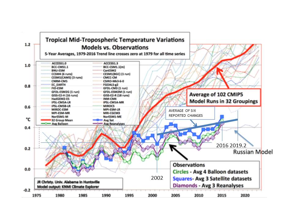 demonstrated that the GCMs are wrong and this paper corroborates that by showing that GCMs have no predictive value. Contribution from CO2, if any, is completely masked by other uncertainties.
Several examples of compelling evidence CO2 has no effect on climate are listed in Section 2 of http://globalclimatedrivers2.blogspot.com . Included also in that analysis is an explanation of WHY CO2 has no significant effect on climate and evidence. Calculations in Section 8 show that water vapor has been increasing about twice as fast as indicated by the temperature increase of the liquid water. The extra increasing water vapor, provided by humanity, has contributed to the rise in average global temperature since the depths of the LIA.
“water vapor has been increasing about twice as fast as indicated by the temperature increase of the liquid water.
That particular forcing is part of the standard global warming theory, atmospheric CO2 changing the energy budget over the decades, warming the oceans and creating these kinds of massive feedback.
The main challenge would be to provide a better theoretical basis for the origin of the increase of water temperature. It’s not clear to me if you’re providing any and yet I’m skeptical of AGW theories too.
JD,
You have been grievously deceived. The water vapor increase resulting from temperature increase is easily calculated from the vapor pressure vs temperature relation. The standard global warming theory assumes that WV increases only as indicated by the temperature increase.
The observation is that, at least since it has been accurately measured worldwide, it has been increasing about TWICE that. Therefore, WV increase is driving temperature increase, not the other way around. Calculations are provided in Section 8 of my blog/analysis http://globalclimatedrivers2.blogspot.com .
I did extensive research into where the extra WV comes from. It is documented in Section 9. The WV increase results mostly (about 86%) from irrigation increase.
NASA/RSS have been measuring water vapor by satellite and reporting it since 1988 at http://www.remss.com/measurements/atmospheric-water-vapor/tpw-1-deg-product . Fig 3 in my b/a is a graph of the NASA/RSS numerical data. When normalized by dividing by the mean, the NASA/RSS data are corroborated by NCEP R1 and NCEP R2.
Pat, in digital simulation , we run min max simulations to ensure our electronic circuitry will run correctly under all expected circumstances. This would, if implemented within climate modelling, mean that each climate run would involve a separate run with each variable at each end of its range. So a million run -4watts, max run +4 watts etc and see that a) the model does not break and b) the error bars are acceptable.
I expect both a) and b) both fail.
Likely, and you put your finger on an important and unappreciated point, Steve.
This is that climate models are engineering models, not physical models.
Their parameters are adjusted to reproduce observables over a calibration period.
A windsteam model for example, is adjusted by experiment to reproduce the behavior of the air stream over an airfoil across its operating specs and some degree of extreme. It can reproduce all needed observables in that calibration bound.
But its reliability at predicting beyond that bound likely diminishes quickly. No engineer would trust an engineering model used beyond its calibration bounds.
But every climate projection is exactly that.
Pat,
Your mention of calibration chimed a memory with me. I was reminded of the Tiljander upside-down calibration issue and so I went looking on Climate Audit. There I found this comment by you dated 17 Oct 2009.
https://climateaudit.org/2009/10/14/upside-side-down-mann-and-the-peerreviewedliterature/#comment-198966
You have been fighting this battle for a long time now.
Duh, This one:-
https://climateaudit.org/2009/10/14/upside-side-down-mann-and-the-peerreviewedliterature/#comment-198987
Extrapolating beyond calibration end-points for a high-order polynomial fit is commonly recognized to be highly unreliable.
Pat, thank you for your careful analysis of my comments further upthread. I am repeating them here annotated with #, and then replying to them.
#See – Owe to Rich, first, you appear to be confusing physical error with uncertainty.
Well, future uncertainty represents a range of plausible physical errors which will occur when that time arrives. So I think it’s just semantics, but let’s not dwell on it.
# Second, I do not “ show that errors in TCF (Total Cloud Fraction) are correlated with latitude” rather I show that TCF errors are pair-wise correlated between GCMs.
Well, Figure 4 shows to they eye that those errors are correlated with latitude, but if that isn’t what you actually analyzed then fair enough. In your “structure of CMIP5 TCF error” you didn’t specify what the x_i were, and I mistook them for latitude rather than a model run.
#Third and fourth, I do not “derive, using work of others, a TCF error per year of 4Wm^-2”.
The ±4W/m^2 is average annual long wave cloud forcing (LWCF) calibration error statistic. It comes from TCF error, but is not the TCF error metric. The LWCF error statistic comes from Lauer and Hamilton. I did not derive it.
OK, semantics again, but they can become important, so I’ll use “LWCF calibration error” from now on.
#Fifth, eqn. 4 does not involve any lag-1 component. It just gives the standard equation for error propagation. As the ±4W/m^2 is an average calibration statistic derived from the cloud simulation error of 27 GCMs, it’s not clear at all that there is a covariance term to propagate. It represents the average uncertainty produced by model theory-error. How does a 27-GCM average of theory-error co-vary?
OK, but the x_i’s here are time, are they not, as we are talking about time propagation? So where x_i and x_{i+1} occur together it is not unreasonable to refer to this as a lag, again it is semantics. And across time intervals, covariation is highly likely.
# Sixth, your “ n years the error will be 4sqrt(n) Wm^-2.” the unnumbered equation again lays out the general rule for error propagation in more usable terms. The u_a … in that equation are general, and do not represent W/m^2. You show a very fundamental mistaken understanding there.
Well, your use of the u_a’s certainly does have some dimension, which I took to be W/m^2, but I now see that it is Kelvin as you talk about “air temperature projections”.
# Seventh, your, “after 81 years that would give 36 Wm^-2,” nowhere do I propagate W/m^2. Equations 5 and 6 should have made it clear to you that I propagate the derived uncertainty in temperature.
Yes, OK, in 5.1 you do convert from the 4W/m^2 into u_i in Kelvins via a linear relationship. It is however true that if we remained in W/m^2 we would indeed reach 36W/m^2 after 81 years. But I’m happy to convert to K first.
# Eighth, your “So I do now see how your resulting large error bounds are obtained. ” It’s very clear that you do not. You’ll notice, for example that nowhere does a sensitivity of 2K or of anything else enter anywhere into my uncertainty analysis. Your need to convert W/m^2 to temperature using a sensitivity number fully separates my work from your understanding of it.
No, really, I do. Whatever units we are working in, an uncertainty E has become, after 81 years, 9E. And actually, though you don’t realize it, you do have an implicit sensitivity number. It is 33*f_CO2*D/F_o = 33*0.42*3.7/33.3 = 1.54K. Here D is the radiative forcing from a doubling of CO2, which IPCC says is 3.7W/m^2, and the other figures are from your paper.
# Ninth, your subsequent analysis in terms of error (“So one flaw … greater flaw as I see it is that global warming is not wholly a cumulative process….) shows that you’ve completely missed the point that the propagation is in terms of uncertainty. The actual physical error is completely unknown in a futures projection.
Semantics again.
# Tenth, your, “hence suffer less error than you predict.” I don’t predict error. You’ve failed to understand anything of the analysis.
I think I’ve understood a lot, thanks.
#Eleventh “Apparently your peer reviewers didn’t spot that point.” because it’s not there. It’s wrong, it exists in your head, and it’s nowhere else.
Yes, that was a bit snarky of me. But I don’t think your use of the error propagation mathematics is correct. Of these eleven points, the fifth one is the only one which really matters and is at the heart of my criticism. I need to go away and do a bit of mathematics to see if I can substantiate that, but ignoring covariance is, I think, the key to the problem. This is certainly interesting stuff.
See, you wrote, “Well, future uncertainty represents a range of plausible physical errors…”
No, it does not. You may dismiss the distinction as semantics, but the difference between error and uncertainty is in fact central to understanding the argument.
You wrote”you didn’t specify what the x_i were, and I mistook them for latitude rather than a model run.”
Here’s how I described the x_i: “For a data series, x_1, x_2,. . . , x_n, a test for lag-1 autocorrelation plots every point x_i against point x_i_1.”
That looks live a very specific description of the x_i to me. And it describes neither a latitude nor a model run.
You wrote regarding the error statistic coming from Lauer and Hamilton, , “OK, semantics again…” That’s the second of your important mistakes you’ve dismissed as mere semantics. How convenient for you.
You wrote, “OK, but the x_i’s here are time …” No, they’re latitude. Look at Figure 5, where the lag-1 plot is shown.
You wrote, “but I now see that it is Kelvin as you talk about “air temperature projections”. The unnumbered equation has no units. It’s a generalized equation. It’s not Kelvins.
You say that “The actual physical error is completely unknown in a futures projection.” is “semantics again. Incredible. It’s mere semantics that physical error is unknown in a futures projection.
Our complete ignorance of the size of the error is why we take recourse to uncertainty.
It’s quite clear that your understanding of the argument in the paper is sorely deficient, See.
Pat, a mathematical equation to describe what you are doing is, I think,
T_i(t) = T_i(t-1) + d_i(t) + e_i(t)
where i is the model number, T_i(t) is temperature at time (year) t, d_i(t) is a non-stochastic increment, and e_i(t) is an error. Then let T(t) = sum_{i=1}^n T_i(t)/n. I don’t accept this as a good summary of the GCMs, but let’s see what it implies. Assume that T_i(t-1) is uncorrelated with e_i(t), and that e_i(t) is uncorrelated with e_j(t) for i!=j. Then
Var[T(t)] = Var[T(t-1)] + sum_i Var[e_i(t)]/n^2 (*)
Now it is possible that e_i(t) to have a structure like e_i(t) = (i-(n+1)/2)a(t) + b_i(t) where a(t) is non-stochastic and b_i(t) has very small variance. In this case Var[e_i(t)] = Var[b_i(t)] in (*) above, and the growth of Var[T(t)] against t is then very small.
Can you prove that something like this is not the case? (I haven’t read the SI to see whether this is covered.) It would be saying that each model i has a bias regarding TCF which does not vary much from year to year. That seems plausible to me, but some torturing of data should reveal the truth.
Look at the figures in Lauer and Hamilton, 2013, See. The model errors are not offset biases.
Your equation is not what I’m doing. The physical errors in projected temperatures are not known.
Annually projected temperature changes are calculated from annual changes in forcing. Their value has no dependence on the magnitude of prior temperature.
Also, uncertainties are not errors. Why is that distinction so invisible to you?
Dr Frank,
I read your paper.
I read the SI.
I watched the video of Dr Patrick Brown.
I read through your exchange of comments with Dr Patrick Brown.
On balance, I am unconvinced by your paper, even though I can list the multiple reasons why AOGCMs have little useful predictive ability.
I have a major concern with your use of a memoryless model to emulate the GCMs, although the problems arising from this are swamped by the larger question of whether it is legitimate to accumulate uncertainty in forcing, and hence temperature, by adding independent samples year-on-year from a distribution with a standard deviation of 4W/m2, as derived from your “global annual cloud simulation calibration error statistic”. In the derivation of this latter statistic, you make no attempt to distinguish between systemic bias and other sources of difference. This is fatal. The distinction is critical to your subsequent uncertainty estimation, and it needs to be founded on individual within-model distinction, before any between-model aggregation or averaging.
To illustrate the point, let us say hypothetically that there is exactly a fixed difference of X in cloud-cover units between every “observed point” and every modeled point (binned at whatever temporal interval you choose), used to derive your calibration data.
Your analysis would translate this difference, X, into a non-zero year-on-year forcing uncertainty of plus or minus Y W/m2. Let us say Y = 4 W/m2 for convenience in this hypothetical example.
Your uncertainty analysis would then yield exactly the same final uncertainty envelope that you display, if I have understood your approach.
However, in the corresponding AOGCM model, while this type of systemic difference in cloud cover is certainly a source of error, the uncertainty in temperature projection which it introduces FROM FORCING UNCERTAINTY is close to zero. (It does introduce a different uncertainty related to the sensitivity of the system to a given forcing, which is quite different, and which most certainly cannot be estimated via adding independent forcing uncertainties in quadrature year-by-year.)
Every AOGCM by prescription produces Pre-Industrial Control runs (“PI control”) for upto 500 years. When a modeling group initiates a run like a 1% per year quadrupling of CO2 or a 20th Century Historical run, the kick-off start-times for multiple runs are selected from time-points towards the end of these runs to allow some variation in initial conditions. The temperature CHANGES and net flux CHANGES from the start-year for each run are then estimated by taking the difference between the run values and the PI Control values at the kick-off point for that run. The temperature and net flux values are then averaged across the multiple runs to produce the data which, for example, you have used in your emulator comparison tests.
The point is that any net flux error arising from a systemic error in cloud cover is already present at the start of the AOGCM run, at which point the system is very close to a net flux balance. All forcing drivers applied thereafter are being applied to a system close to a net flux balance. The systemic cloud error therefore has zero effect on subsequent forcing uncertainty. Since, however, the net flux balance itself is likely to be spurious because of the need for compensation of the systemic error in cloud cover, the sensitivity of the system is probably affected; but this is a different type of uncertainty, with a very different form and propagation characteristics, from the forcing uncertainty which you are purporting to estimate.
Somewhat ironically, one of the arguments used for the comparison of cloud cover averages over different time intervals was that the modeled values were changing slowly. Your paper would be a lot more convincing if you could show in analysis of the cloud cover data that you were specifically attempting to eliminate any systemic difference, since its contribution to forcing uncertainty should be close to zero.
kribaez, that is very interesting. I think you are reinforcing the concerns I have stated above. Your “systemic error in cloud cover” sounds (after converting from W/m^2 to K) like my example (i-(n+1)/2)a(t), where a(t) is non-stochastic and the mean over the n models is zero. Then with “the modeled values were changing slowly” we get b_i(t) with small variance, and it is these small variances (divided by n^2) which can be added to provide the variance growth in projection uncertainty over time.
Does that make sense to you?
The key in Frank’s error propagation is recursive model calculations of everything. I’m not at all sure that GCMs actually do that.
See,
I suspect your n^2 should be n, but yes something like that. My main point was restated by Roy Spencer who must have read my post before commenting (sarc). The forcing value which appears in Pat Frank’s emulator is by definition an induced change in NET FLUX at TOA (or sometimes defined at the top of the climatological troposphere). Any constant offset error in LW cloud forcing is already neutralised by a combination of valid offset (covarying SW) and by compensating errors before any of the AOGCMs start a run. We may not know where the compensating errors are but we know they are there because the TOA net flux is (always) close to being in balance at the start of the run. Such a constant offset difference in LCF between model and reality clearly introduces both error and uncertainty, but by no stretch of the imagination can it be treated as though it were a calibration error in forcing, which is what Dr Frank is doing.
±4W/m^2 is not a constant offset, kribaez.
Nor is it an induced change in net forcing. It is the uncertainty in simulated tropospheric thermal energy flux resulting from simulation error in total cloud fraction.
None of you people seem to understand the meaning or impact of a calibration experiment or of its result.
Dr Frank,
For someone who complains so often about the reading skills and knowledge base of others, you might look to the beam in your own eye. What I invited you to consider was that if there existed such a hypothetical systemic offset, your calibration exercise would include such an offset as part of your estimated forcing uncertainty, despite the fact that it is a completely different animal and absolutely cannot be sensibly propagated as you propagate your forcing uncertainty.
I’ll just quote this one line, because it encapsulates the core of your argument, kribaez: “The point is that any net flux error arising from a systemic error in cloud cover is already present at the start of the AOGCM run, at which point the system is very close to a net flux balance.”
And your equilibrated climate has the wrong energy-state. We know that because the deployed physical theory is incomplete, at the least, or just wrong. Or both.
You’re claiming that the errors subtract away.
However, your simulated climate is projected as state variables, not as anomalies. That means the initial incorrect climate state is further incorrectly projected.
The errors in simulated climate state C_i+1 will not be identical to the errors in C_i, because the extrapolation of an incorrect theory means that output errors further build upon the input errors.
Subtraction of unknown errors does not lead to perfection. It leads to unknown errors that may even be larger than the errors in the differenced climate state variables.
That’s the horror of systematic errors of unknown magnitude. All of physical science must deal with that awful reality, except, apparently, climate modeling.
You say that you read the paper and the SI. This point is covered in detail. Somehow, you must not have seen it.
My emulator comparison tests used the standard IPCC SRES and RCP forcings. And you’ll note that the comparisons were highly accurate.
Also, I estimated no forcing uncertainty. I obtained the LWCF error from Lauer and Hamilton, 2013. What I estimated was a lower limit of reliability of the air temperature projections.
Dr Frank,
“And your equilibrated climate has the wrong energy-state. We know that because the deployed physical theory is incomplete, at the least, or just wrong. Or both.” I agree.
“You’re claiming that the errors subtract away. ” No I am certainly not. I am saying (for the third time, I think) that the errors introduced by a hypothetical constant offset error in cloud coverage do not propagate in the way you have propagated your “forcing uncertainty”, but since you have made no attempt to separate out such error in your calibration, your forcing uncertainty includes and propagates all such error.
“My emulator comparison tests used the standard IPCC SRES and RCP forcings. And you’ll note that the comparisons were highly accurate.” Mmm. I mentioned somewhere above that I was concerned about your use of this emulation model, but decided not to elucidate. I will do so now.
Let me first of all make a statement of the obvious. The forcing term which you use in your emulation equation is a forcing to a net flux, not a net flux. More explicitly, the forcing terms in this equation can be thought of as deterministic inputs (the real inputs are deterministic forcing drivers which are converted by calculation to an instantaneous forcing – an induced or imposed CHANGE in net flux ). These inputs do not include LW cloud forcing; it is NOT an input in this sense. It is one of multiple fluxes which collectively define the climate state in general and the net flux balance in particular. To define the uncertainty in temperature projection, you need to define the uncertainty in net flux (and capacities inter alia).
Your linear relationship describing temperature as a function of forcing can be derived in several ways. One such way is I think important because it starts with a more accurate emulation device than yours, but can be shown to yield your approximation with some simplifying assumptions.
The AOGCMs are known to be close to linear systems in their behaviour. A doubling of a forcing profile results in a doubling of the incremental temperature response profile, and at long timeframes, equilibrium temperature can be expressed as a linear function of the final forcing level. Your model reflects that. More generally, their transient behaviour can be very accurately emulated using an LTI system based on energy balance. For a constant forcing, F, applied at time t = 0, the net flux imbalance N(t) is given exactly by:-
N(t) = Input flux(t) – Output flux(t) = Input flux(0) + F – Output flux(0) – Restorative flux(T,t) (1)
For simplicity, here I will assume a constant linear feedback, γ ΔT, for the restorative flux, although the argument can be extended to cover a more general condition.
Restorative flux (T,t) = γ ΔT where ΔT is the CHANGE in GSAT since t=0.
This yields
N(t) = F – γ ΔT + Input flux (0) – Output flux(0) (2)
If the system starts in steady-state at time t=0, then irrespective of the form of N(t), providing only that it is definable as a linear system in T, we have that T -> F/ γ at long timeframes, since (N ->0). So were does a constant offset error in cloud fraction manifest itself ? It appears here in both the input and output flux at time zero. Let us say that it introduces a net flux error of +4W/m2 downwards. This may be from downward LW or any other cloud-associated flux.
Assuming zero external forcing during the spin-up, Equation 2 becomes
N(t) = 0 – γ ΔT + 4
After 500 years of spin-up, ΔT-> 4/ γ , and the system is a little bit warmer than it was 500 years previously, and it is now back in balance for the start of the 20th century historic run. There is no justification whatsoever for propagating this forwards as though it were the same as a year-on-year uncertainty in forcing or net flux imbalance, which is what you are doing.
There IS justification for describing it as an error and a source of uncertainty, but your treatment of its associated uncertainty seems entirely inappropriate.
kribaez, you wrote, “I am saying (for the third time, I think) that the errors introduced by a hypothetical constant offset error in cloud coverage do not propagate in the way you have propagated your “forcing uncertainty”…”
There is no constant offset error. Take a look at Lauer and Hamilton. All the models show positive and negative error regions.
Those positive and negative errors are combined into a rms global error. That is, ±e. Not +e nor -e.
Confining your analysis to terms of a constant offset error is wrong.
You wrote, “The forcing term which you use in your emulation equation is a forcing to a net flux, not a net flux.
The forcing enters the net flux. The simulation uncertainty — the calibration error — in the net flux establishes the limit of resolution of the model.
That resolution limit is a bound on the accuracy of any simulation. It propagates into sequential calculations. The uncertainty grows with each step. You can’t get around it.
I wonder if some colleagues at SLAC, and elsewhere, would apply this thorough analysis to fusion plasma, likely one of the most difficult areas.
I shudder to think if the delays are due to such errors.
Could it be the climate crew are making mistakes that are systematic in other areas too?
Dr. Frank: “Nick argues for +4W/m^2 rather than the correct ±4 W/m^2 to give false cover to folks like ATTP who argue that all systematic error is merely a constant offset.”
I actually thought the ‘constant offset’ part of Brown’s presentation was a pretty weak analogy, although admittedly I may be missing something important. To me that approach seems to equate to a one-time error in initial conditions; whereas intuitively an error in LCF seems more to be a boundary issue that would have impact as the model steps through time…which would seem correct that the uncertainty would compound over time in some fashion (in annual chunks, 20 year chunks, or continuously, depending on how the +/- 4 w/m^2 is determined).
“all systematic error is merely a constant offset” Especially true of the adjusters at NOAA, but theirs is an example of a systematic error that propagates continuously, and always in the same direction.
Dr. Spencer has posted an article on the paper.
https://www.drroyspencer.com
I look forward to Pat’s reply to Dr. Spencer.
I just do not have the required knowledge to get at this, but something about the following statement of Dr. Spencer raises some flags:
I have replied to Dr. Spencer, Robert.
As you’ll see, he makes so many fundamental mistakes as to remove any critical force from his comments.
Unfortunately, his site does not support the “±.” So, none of them came through in my reply. I had to add a corrective comment after posting to alert readers to this problem.
And it was good reply.
I sensed a bunch of erroneous thinking there in Roy’s analysis, but, again, I lack the knowledge-skill to express the errors, or even understand them fully.
Nonetheless, I remain convinced of the conclusions reached in your paper, PF. I also feel certain that you will have to go through this many more times, with many more people. I hope you’re up for the ensuing ultra-marathon. (^_^) … I’ll be watching, as it unfolds.
After 6 years, 13 submissions, 30 reviewers I think Dr Frank is the Ultra-Marathoner of climate science.
And Dr Frank’s reply is in the comments.
Dr. Spencer is basing his comments upon the actual model behavior, and is ignoring the uncertainty behind the calculations. It is uncertain how cloud behavior really changes when various physical changes happen. The models might accidentally emulate reality, but the mathematical uncertainty remains, and we don’t know how far the model predictions are from what will really happen.
“Dr. Spencer is basing his comments upon the actual model behavior…”
Of course he is! All error propagation is model-dependent. All uncertainty analysis of any output is dependent on the knowledge-space of inputs, validity of model governing equations AND model-dependent error propagation. You cannot get away from the model. Pat’s own work uses a model when he estimates uncertainty based on an emulator of AOGCM results. Roy Spencer’s comments are suggesting that Pat is incorrectly translating an estimated uncertainty in one particular flux, which has close to a 100% compensatory error in the AOGCM, into a bald propagating uncertainty in the net flux imbalance, which is what Pat does when he attaches this uncertainty to his “forcing”. This is not credible. The AOGCM cannot and does not propagate a flux error arising from cloud fraction error as though it were the same thing as a forcing error. You do not need a degree in statistics to understand this.
Try this grossly oversimplified model. A is all incoming flux prior to any forcing. B is all outgoing flux prior to any forcing. N is the net flux imbalance (which is what actually controls temperature change).
N = A – B + F where F is a forcing to the net flux.
B = A with a correlation of 1.
A has a variance of VAR(A). B has a variance of VAR(B) = VAR(A).
Forcing is a deterministic input:- VAR(F) = 0
Under normal statistical rules:-
Var(N) = Var(A) + Var(B) – 2 COV(AB) = 0
Pat’s model examines only the variance of A, without taking any account the compensating correlated value of B. He is in effect saying Var(N) = Var(A+F) = VAR(A)
This is not kosher. In truth, Pat is not doing quite what this model suggests, but it is close and serves to illustrate the key point that Roy Spencer is making.
Windchaser, “Roy Spencer’s comments are suggesting that Pat is incorrectly translating an estimated uncertainty in one particular flux, which has close to a 100% compensatory error in the AOGCM, into a bald propagating uncertainty in the net flux imbalance, which is what Pat does when he attaches this uncertainty to his “forcing”.”
No, that isn’t what Pat does.
You’re equating an uncertainty with a physical error, Windchaser. Big mistake.
The uncertainty is ±4 W/m^2. How is a ±value compensated? No offsetting error can compensate a ±value. Taking a difference merely goes from plus/minus to minus/plus.
You’re basically making the same mistake Roy is: you’re supposing that a calibration uncertainty statistic is an energy flux error. It’s not. That mistake invalidates your analysis.
You wrote, “The AOGCM cannot and does not propagate a flux error arising from cloud fraction error as though it were the same thing as a forcing error. You do not need a degree in statistics to understand this.”
My paper does not discuss physical flux errors that impact simulations. There is nothing for an AOGCM to propagate in a calibration error statistic. The calibration error statistic is not part of any simulation.
You wrote, “Pat’s model examines only the variance of A…”
No, it does not.
Let’s use your simple model to illustrate what’s actually going on, Windchaser. You neglect certain uncertainties.
Corrected, your incoming is A±a and outgoing is B±b. Forcing F is defined in a scenario and is an assigned value with no uncertainty.
Then the uncertainty in the difference, A±a – B±b, is the combined uncertainty of the values entering the difference: sqrt(a^2+b^2) = ±n.
Following from that, A±a – B±b + F = N±n. Your net flux is N±n. When A = B then N = F, and F inherits the uncertainty in N. Every forcing is F±n.
Now we calculate the resulting air temperature from the change in forcing, F±n. The calculated uncertainty in the temperature change reflects the impact of the forcing uncertainty, ±n, and is T±t.
The simulation goes exactly as before, providing discrete values of T for the assigned values of F. The effect on uncertainty due to the ±n conditioning the assigned forcing F is calculated after the simulation is complete.
Now you simulate a future climate knowing that every single F is conditioned with a ±n.
The first step calculates a T_1, which has an uncertainty of ±t_1 due to ±n. The next step also uses F±n to calculate T_2. That value is (T_2)±t_2.
The temperature change at the end of the two steps is the sum of the changes, T_1+T_2, call it T_II.
The uncertainty in T_II is the root sum square of the uncertainties in the two step-calculation: sqrt[(t_1)^2+(t_2)^2] = ±t_II.
So, after two steps our temperature change is (T_II)±t_II, and ±t_II > ±t_1 and ±t_2.
And so it goes for every step. If ±n is constant with each step, then the ±t at each step is constant. After Q steps, the uncertainty in the projected temperature is sqrt[Q x (±t)^2] = ±t_q, and the final temperature is T_Q±t_q. The ±t_q >>> ±t.
None of that is involved in the simulation.
There is nothing for the AOGCM to compensate.
The simulation goes on as before, with TOA balance, discrete expectation values, and all.
However, the growth of uncertainty means that very quickly, the temperature projection loses any physical meaning because ±t_q rapidly becomes very large.
When ±t_q is very large, the T_Q±t_q has no physical meaning. It tells us nothing about the state of the future climate.
Pat,
I think you are blaming Windchaser for my faults.
“You’re basically making the same mistake Roy is: you’re supposing that a calibration uncertainty statistic is an energy flux error. It’s not. That mistake invalidates your analysis.” I knew that I would eventually end up on this growing list.
Staying with the oversimplified example, you wrote:-
“Then the uncertainty in the difference, A±a – B±b, is the combined uncertainty of the values entering the difference: sqrt(a^2+b^2) = ±n.”
The illustrative example specified a correlation of 1.0 between A and B. They co-vary perfectly by assumption. What you have written is therefore nonsense.
If your value of “a” is independently estimated as a sd or an RMSE from calibration data against A, then what you have written is still total nonsense. The uncertainty in the difference is zero, prescribed by the assumption, and the uncertainty in A cannot propagate, despite the apparent calibration error. The covariance is equal to the variance of A which is equal to the variance of B. The difference is zero and the variance of the difference is zero.
The real problem, of course, does not have a perfect correlation between A and B, however, in the absence of external forcing, A-B must drift with small error around zero in the AOGCMs by virtue of the governing equations on which they are based.
Your analysis, however, does not consider the calibration of A, nor the calibration of B, nor the calibration of A-B. Instead, it considers just one flux component which goes into B, and since the sum of all such components must be equal to B, and A-B is bounded, then we can deduce that any error in net flux introduced by this component is largely offset at start-of-run by errors in the other components, such that A-B remains bounded.
kribaez, you’re right, thanks. It was your comment, not Windchaser’s
Apologies to Windchaser and to you. 🙂
You wrote, “The illustrative example specified a correlation of 1.0 between A and B. They co-vary perfectly by assumption. What you have written is therefore nonsense.”
The illustrative example specified A = B with a correlation of 1. Therefore A-B is always 0.
I added uncertainty limits around A and B to make them real-world, rather than your Platonic, ‘perfect knowledge’ model. Adding uncertainties makes your example a useful illustration of what I actually did.
You wrote, “The uncertainty in the difference is zero, prescribed by the assumption, and the uncertainty in A cannot propagate, despite the apparent calibration error.”
Your assumption presumed perfect knowledge of the magnitudes of A and B. You can assume that, of course, but that makes your example useless and completely unrealistic and inapplicable to illustrate an uncertainty analysis.
In fact, if A and B have uncertainties associated with them, then the uncertainty propagates into their difference as I showed.
In Bizzaro-world where everyone knows everything to perfect accuracy and to infinite precision, your ideas might find application. Everywhere else, no.
You wrote, “The covariance is equal to the variance of A which is equal to the variance of B. The difference is zero and the variance of the difference is zero.”
In Bizzaro-world. Not here, where there are limits to measurement resolution, to knowledge, and to the accuracy of physical description.
Neither you nor anyone else can know A and B to perfection. Even if we had a physical theory that said they do vary in perfect correlation, our knowledge of their magnitudes would include uncertainties. That is, A±a and B±b. Then , A±a – B±b = N±n.
Your insistence on an unrealistic perfection of knowledge is hardly more than self-serving.
You wrote, “any error in net flux introduced by this component is largely offset at start-of-run by errors in the other components, such that A-B remains bounded.”
You’re equating errors with uncertainty again. Offsetting errors do not improve the physical theory. With offsetting errors., you have no idea whether your physical description is correct. You therefore have no idea of the correct physical state of the system.
Even if you happen to get the right answer, it provides no knowledge of the state of the real physical system, nor does it provide any reassurance that the model will produce other correct answers.
It doesn’t matter that A-B is bounded. The uncertainty grows without bound as the ±n propagates into and through a sequential series of calculations.
That means there are huge uncertainties in the physical description of your system that are hidden by offsetting errors.
All offsetting errors compound in quadrature to produce an overall uncertainty in the calculation.
Take a look at sections 7 and 10 in the SI, where I discuss these issues at some length.
A spin-up equilibrated simulated climate C_0 is an incorrect representation of the energy-state of the system.
Model theory-error means that the incorrect base-state climate is further incorrectly simulated. The errors in simulated climate C_1 are not known to be identical to those in base-state simulation C_0.
None of the errors are known in a futures prediction. All one can do is use uncertainty analysis to estimate the reliability of the projection. And the uncertainty grows without bound.
Dr Frank,
Thank you for this last response. I now fear that you may be labouring under a serious conceptual misunderstanding.
I would strongly urge you to re-examine what you wrote in your discussion of the law of propagation of uncertainty:- your Equations S10.1 and S10.2.
When I encountered your Equation S10.2, on first reading your SI, I thought that you had just been sloppy with your qualification of its applicability, since, as written, it is only applicable to strictly independent values of x_i . I found it difficult to believe that the NIST could carry such an aberrant mis-statement for so long, so I returned to the Taylor and Kuyatt reference, and found that it did correctly include the covariance terms, which for some inexplicable reason you had dropped with a note saying:-
“The propagation equation S9.2 (sic) appears identically as the first term in NIST eq. A3”
I am at a complete loss to understand why you dropped the covariance terms, but if you believe, as your above response seems to suggest, that var(A-B) = var(A) + var(B) when A and B covary with a correlation coefficient of 1, then that would explain quite a lot about your rejection of the offset error argument.
It would also explain why you think it is reasonable to accumulate the full variance of your forcing uncertainty statistic without accounting for autocorrelation from year to year.
Can you please reassure me that you do understand that your S10.2 is a mis-statement as it stands?
kribaez, I ignored covariance because the LWCF error is a multi-year, multi-model calibration annual average uncertainty for CMIP5 models.
As a static multi-model multi-year average, it does not covary with anything.
Equations S10.1 and S10.2 are exactly correct.
This illustration might clarify the meaning of the (+/-)4 W/m^2 of uncertainty in annual average LWCF.
The question to be addressed is what accuracy is necessary in simulated cloud fraction to resolve the annual impact of CO2 forcing?
We know from Lauer and Hamilton that the average CMIP5 (+/-)12.1% annual cloud fraction (CF) error produces an annual average (+/-)4 W/m^2 error in long wave cloud forcing (LWCF).
We also know that the annual average increase in CO2 forcing is about 0.035 W/m^2.
Assuming a linear relationship between cloud fraction error and LWCF error, the (+/-)12.1% CF error is proportionately responsible for (+/-)4 W/m^2 annual average LWCF error.
Then one can estimate the level of resolution necessary to reveal the annual average cloud fraction response to CO2 forcing as, (0.035 W/m^2/(+/-)4 W/m^2)*(+/-)12.1% cloud fraction = 0.11% change in cloud fraction.
This indicates that a climate model needs to be able to accurately simulate a 0.11% feedback response in cloud fraction to resolve the annual impact of CO2 emissions on the climate.
That is, the cloud feedback to a 0.035 W/m^2 annual CO2 forcing needs to be known, and able to be simulated, to a resolution of 0.11% in CF in order to know how clouds respond to annual CO2 forcing.
Alternatively, we know the total tropospheric cloud feedback effect is about -25 W/m^2. This is the cumulative influence of 67% global cloud fraction.
The annual tropospheric CO2 forcing is, again, about 0.035 W/m^2. The CF equivalent that produces this feedback energy flux is again linearly estimated as (0.035 W/m^2/25 W/m^2)*67% = 0.094%.
Assuming the linear relations are reasonable, both methods indicate that the model resolution needed to accurately simulate the annual cloud feedback response of the climate, to an annual 0.035 W/m^2 of CO2 forcing, is about 0.1% CF.
To achieve that level of resolution, the model must accurately simulate cloud type, cloud distribution and cloud height, as well as precipitation and tropical thunderstorms.
This analysis illustrates the meaning of the (+/-)4 W/m^2 LWCF error. That error indicates the overall level of ignorance concerning cloud response and feedback.
The CF ignorance is such that tropospheric thermal energy flux is never known to better than (+/-)4 W/m^2. This is true whether forcing from CO2 emissions is present or not.
GCMs cannot simulate cloud response to 0.1% accuracy. It is not possible to simulate how clouds will respond to CO2 forcing.
It is therefore not possible to simulate the effect of CO2 emissions, if any, on air temperature.
As the model steps through the projection, our knowledge of the consequent global CF steadily diminishes because a GCM cannot simulate the global cloud response to CO2 forcing, and thus cloud feedback, at all for any step.
It is true in every step of a simulation. And it means that projection uncertainty compounds because every erroneous intermediate climate state is subjected to further simulation error.
This is why the uncertainty in projected air temperature increases so dramatically. The model is step-by-step walking away from initial value knowledge further and further into ignorance.
On an annual average basis, the uncertainty in CF feedback is (+/-)144 times larger than the perturbation to be resolved.
The CF response is so poorly known, that even the first simulation step enters terra incognita.
I am a simple EE so if I am a little off base here be gentle in your criticisms.
==========================================
Dr. Spencer –>
“Climate Models Do NOT Have Substantial Errors in their TOA Net Energy Flux
If any climate model has as large as a 4 W/m2 bias in top-of-atmosphere (TOA) energy flux, it would cause substantial spurious warming or cooling. None of them do.”
…
“The reason is that the +/-4 W/m2 bias error in LWCF assumed by Dr. Frank is almost exactly cancelled by other biases in the climate models that make up the top-of-atmosphere global radiative balance.”
===============================================
This doesn’t seem to be a proof that there isn’t a 4 W/m2 bias derived from TCF.
It seems more a proof that there is an error, but it is offset by other errors in the models.
In the end, accumulated errors may offset each other which seems to validate the linear basis of his model. Yet it doesn’t disprove that individual errors accumulate.
================================================
Systematic errors do accumulate. I’ve already used an example where if you measure a long distance divided into ten segments, five of 10 cm and 5 of 20 cm, with a device that only measures each segment that the errors accumulate.
If the first segment is measured as 10 cm +/- 1 cm and then added to a measurement of the second element of 20 cm +/- 1 cm the error doesn’t stay +/- 1 cm. The uncertainty of the result is really +/- 2 cm. So you end up with a total of 30 cm +/- 2 cm. After measuring the ten segments you will end up with a measurement of 150 cm +/- 10 cm. Your result will have a large uncertainty of what the actual measurement is.
This is not variance or standard deviation or error of the means. It is uncertainty of what the end result actually is. As long as a model uses one calculation to feed another calculation, the uncertainty will accumulate.
And the uncertainty does accumulate here, too, but not as Pat Frank describes.
Most importantly: the uncertainty does not accumulate through time, without end. Rather, the static uncertainty in W/m2 forcing results in a static uncertainty in Earth temperature.
No, it doesn’t Windchaser, because the uncertainty derives from a model calibration error. It invariably enters every simulation step.
I discuss this in the paper. The uncertainty necessarily propagates forward.
Error is bounded. Uncertainty grows without limit.
In your second comment, you’re confusing error with uncertainty. This is a common mistake among my critics.
You can’t know the error in a futures projection. You’re left only with an uncertainty.
To put it another way: actual uncertainties in forcing result in *convergent* errors in temperature. This works the same in models and in the real world: if you perturb or vary the forcings, you get a finite temperature change in response.
Pat Frank’s model has them result in *divergent* errors. This is unphysical as well as also unrepresentative of model physics.
Isn’t it the climate models that imply divergence, hence that hockey stick ?
Pat is simply pointing out that any model which generates such a hockey stick is doing so because it is diverging exponentially from reality.
In the real world there are negative feedbacks that prevent hockey stick scenarios and those negative feedbacks are wholly missing from the models hence the rapidly developing divergence between reality and the hockey stick.
Pat must be right on purely common sense grounds and all the above attempts to confuse and obfuscate are just chaff blowing in the wind.
As for Roy Spencer I no longer give him much credence because he believes in an isothermal atmosphere developing on a rotating sphere illuminated by a point source of light despite the inevitable density differentials in the horizontal plane which would inevitably lead to convection and a lapse rate slope.
I trust him on his speciality of satellite sensing but not on meteorology.
In accountancy one has the interesting phenomenon of multiple ‘compensating’ errors self cancelling so that one thinks the accounts are correct when they are not.
This is similar.
Many aspects of the climate are currently unquantifiable so multiple potentially inaccurate parameters are inserted into the starting scenario.
That starting scenario is then tuned to match real world observations but it contains all those multiple compensating errors.
Each one of those errors then compounds with the passage of time and the degree of compensating between the various errors may well vary.
The fact is that over time the inaccurate net effect of the errors accumulates faster and faster with rapidly reducing prospects of unravelling the truth.
Climate models are like a set of accounts stuffed to the brim with errors that sometimes offset and sometimes compound each other such that with the passing of time the prospect of unravelling the mess reduces exponentially.
Pat Frank is explaining that in mathematical terms but given the confusion here maybe it is best to simply rely on verbal conceptual imagery to get the point across.
Climate models are currently worthless and dangerous.
This post should stay at the top of WUWT as a first read for newbies to WUWT.
Not all climate modelers get it wrong. R. Pielke , Sr. made a similar point, if slightly less blunt, about model limitations here, here:
https://wattsupwiththat.com/2014/02/07/the-overselling-of-climate-modeling-predictability-on-multi-decadal-time-scales-in-the-2013-ipcc-wg1-report-annex-1-is-not-scientifically-robust/
Climate model projections should be scientific discussion points, not guides for environmental policy.
Sorry for the double “here” My editor(me) failed.
Hey Nick,
And my example above , solar constant. It is a flux, and isn’t quite constant, so people average over periods of time. maybe a year, maybe a solar cycle, whatever. It comes to about 1361 W/m2, whatever period you use. That isn’t 1361 W/m2/year, or W/m2/cycle. It is W/m2.
Que pasa? The same Wikipedia states:
Average annual solar radiation arriving at the top of the Earth’s atmosphere is roughly 1361 W/m^2.
So my understanding is that if there is, say +/-54 W/m^2 uncertainty and this uncertainty is not random but systematic therefore when we do calculation per each year such uncertainty will propagate and accumulate.
Yes, it does accumulate. Integrate a W/m2 uncertainty over time, and you get J/m2. This translates into an expanding uncertainty with regard to energy (Joules) as time goes on, or temperature.
But, the hotter the Earth is, the faster it radiates energy away, and the cooler it is, the slower it radiates energy away. The Stefan-Boltzmann Law acts as a negative feedback on any forcing, and keeps the Earth from just accumulating or losing energy without end. This functionally limits the effects of any new forcing. So the systematic uncertainty in energy flux results in a fixed uncertainty in temperature.
That’s how the physics works out, at least. And you can do Monte Carlo simulations to verify — basically, if you have a physics-based simulation of the climate, even a very primitive one, and you sample forcings within +/- 4W/m2, you’ll find that the results at equilbirium is a range of temperatures. That’s how the uncertainty or perturbation actually propagates through, in both models and real world.
Paramenter:
The Wikipedia description is ill-phrased. Since a Watt is equivalent to one joule per second, an (IMO) more useful expression of the value is ‘roughly 1361 Joules per second per square metre at TOA, when averaged over a year.
“Que pasa? The same Wikipedia states:
Average annual solar radiation arriving at the top of the Earth’s atmosphere is roughly 1361 W/m^2.”
Yes. By annual, they are dealing with the fact that due to elliptical orbit it varies during the year. Because it is periodic, when you say annual, you don’t need to specify a start time.
You could equally take an average over two years. Do you think the answer would be 2722? or 1361?
Hey Nick,
I appreciate that, though Wikipedia wording is not great. How I understand ‘error/time unit’ is that this calibration error can be associated with years as calculations are summarised per year, I believe. So, if a speedometer has systematic error of +10% after one hour drive with a constant speed 20 mph the calculated and actual distance will differ by 2 miles. After another hour by 4 hours. In similar manner I understand Pat argumentation – because calculation of greenhouse gases forcing is summarised yearly yearly uncertainty is also +/- 4 W/m^2/year.
Think you meant “by 4 MILES.”
Interesting article to say the least and possibly the most important.
This approximately translates to 4.7k so therefore all RCP’s included in the models with all temperature rises from between 1.5k to 4.5k are all within the annual average of error.
Roy Spencer coming in, agreeing with Nick Stokes and Ken Rice:
https://www.drroyspencer.com/2019/09/critique-of-propagation-of-error-and-the-reliability-of-global-air-temperature-predictions/#respond
The point is that Dr. Spencer already said this error is offset by other adjustments. Two wrongs don’t make a right. If this error was not offset, what would the uncertainty be? Better yet, how accurate are the predictions when multiple errors are used in calculations?
Plus or minus 4 watts per square meter is not a bias; it is a range of values (errors) extending out to plus and minus 4 from the actual illumination for the time of interest, no ?
Yes 🙂
A concept Nick Stokes repeatedly fails to grasp. And, now, apparently, Dr. Spencer.
I’ll reply to his reply, later this evening.
See my replies on Roy’s blog, Windchasers.
Roy has completely misunderstood the paper. He does not understand error analysis at all.
He thinks an uncertainty in temperature is a physical temperature, and he has dismissed as semantics the difference between energy and a statistic.
Roy is a great guy, but he is really far off the mark.
Nick Stokes thinks that instruments have perfect accuracy and infinite precision. See here and posts following.
That’s how qualified he is to criticize science.
Pat,
To underline your point re the accuracy of instruments, here is one example of how our instrumentation is not exactly what some people think it is.
This is one of my Twitter posts from a few months back, and it shows a graph of the various satellites which have measured TSI over the years.
Each device can give a coherent measurement of changes, but there is little agreement from one device to the next.
I think I have a more up to date graph, but this one gives an idea of the issue…they vary from each other by well over 4 watts/meter squared:
https://twitter.com/NickMcGinley1/status/1142820194781450243?s=20
Good example, Nicholas.
A really striking one, though, is an analytical chemistry paper I once found for Geoff Sherrington.
When the Apollo astronauts brought back moon rock samples, it became very important to determine their mineral and elemental content.
NASA folks were very careful. They sent identical rock samples to several different analytical labs. In the event, as I recall, not one lab reported results even within the uncertainty bounds of results from other labs. It was a revelation about the reality of experimental difficulty.
If Geoff is reading here still, he’ll remember the results better than I.
I have that paper somewhere still.
Pat
I have previously remarked that it is my experience that mathematicians tend to be cavalier about precision and units. I suspect that is true because academics are primarily concerned with teaching mathematical theory and technique, and in doing so, rely a lot on exact integers and unitless numbers with infinite precision and perfect accuracy. I learned more about units and precision in my surveying and chemistry classes than I ever did in my mathematics and physics classes.
I agree, Clyde. Mathematicians live in a kind of Platonic utopia. They focus their attention on problems with closed solutions.
Messy problems are annoyances. One of the real problems in climate modeling is that most of the modelers have degrees in applied or other mathematics.
They seem to have no concept of how to deal with real data, or how messy is physical reality.
When dealing with real data, sometimes ad hoc analytical methods must be developed to get a measure of what one has.
I’m reminded of this quote from Einstein, which really fits the bill: “The reciprocal relationship of epistemology and science is of noteworthy kind. They are dependent upon each other.
Epistemology without contact with science becomes an empty scheme. Science without epistemology is – insofar as it is thinkable at all – primitive and muddled.
However, no sooner has the epistemologist, who is seeking a clear system, fought his way through to such a system, than he is inclined to interpret the thought-content of science in the sense of his system and to reject whatever does not fit into his system.
The scientist, however, cannot afford to carry his striving for epistemological systematic that far. He accepts gratefully the epistemological conceptual analysis; but the external conditions, which are set for him by the facts of experience, do not permit him to let himself be too much restricted in the construction of his conceptual world by the adherence to an epistemological system.
He therefore must appear to the systematic epistemologist as a type of unscrupulous opportunist: he appears as realist insofar as he seeks to describe a world independent of the acts of perception; as idealist insofar as he looks upon the concepts and theories as the free inventions of the human spirit (not logically derivable from what is empirically given); as positivist insofar as he considers his concepts and theories justified only to the extent to which they furnish a logical representation of relations among sensory experiences.
He may even appear as Platonist or Pythagorean insofar as he considers the viewpoint of logical simplicity as an indispensable and effective tool of his research.”
Climate modelers as mathematicians are mostly in the epistemologist camp.
In accountancy one has the interesting phenomenon of multiple ‘compensating’ errors self cancelling so that one thinks the accounts are correct when they are not.
This is similar.
Many aspects of the climate are currently unquantifiable so multiple potentially inaccurate parameters are inserted into the starting scenario.
That starting scenario is then tuned to match real world observations but it contains all those multiple compensating errors.
Each one of those errors then compounds with the passage of time and the degree of compensating between the various errors may well vary.
The fact is that over time the inaccurate net effect of the errors accumulates faster and faster with rapidly reducing prospects of unravelling the truth.
Climate models are like a set of accounts stuffed to the brim with errors that sometimes offset and sometimes compound each other such that with the passing of time the prospect of unravelling the mess reduces exponentially.
Pat Frank is explaining that in mathematical terms but given the confusion here maybe it is best to simply rely on verbal conceptual imagery to get the point across.
Climate models are currently worthless and dangerous.
(Found in the spam bin) SUNMOD
A great description of what is going on. In other words, two wrongs don’t make a right or “x” wrongs don’t make a right.
You’ve outlined the problem well, Stephen.
Apart from my reviewers, I’ve not encountered a climate modeler who understands it.
Pat has emphasised (repeatedly) that ‘uncertainty’ should not be construed as a temperature value. My reading of Roy Spencer’s rebuttal was that he had done just that, and Pat describes it as a basic mistake which he sees being made by many who should know better. We need to have some acknowledgement and resolution on this distinction before we can move forward in any meaningful way. One party has to be wrong and the other right here. Which is it? I’m with Pat
Thank-you, BB.
A statistic is never an actual physical magnitude.
Roy Spencer thinks that the calibration error statistic, ±4 W/m^2, is an energy.
An important exclusion.
Did not contain physical equations that showed any of the warming was related to CO2.
If this was possible it would had been put in writing for all scientists to see regarding actual scientific theory equations that could be tested via scientific method.
Pat Frank’s paper makes scientific predictions which I believe are proper in the sense of being falsifiable. I was thinking about how a CMIP5 model would evolve over time, and how much variance it would have compared to Pat’s predictions, and then it struck me that we should ask the owners to run those models, without tinkering except to provide multiple initial states as desired, and see what happens. Let’s set them up starting with this year’s data, 2019, and run for 81 years to 2100. After all, we do want to know how big that “uncertainty monster” is.
I predict that the standard deviation of model predictions at 2100, which is what I take model uncertainty to mean, will be a lot* less than Pat predicts. Likewise it would be interesting to see whether the uncertainty when using an ensemble of n models is reduced by sqrt(n) or if cross-model correlation makes it worse.
But I may be wrong in my prediction and Pat may be right. Let’s see!
* If this were to go ahead I would attempt to come up with a number to replace “lot”.
See, O2 Rich, your comment shows that you have no concept of the difference between error and uncertainty.
I just received this email. I’ll share it anonymously, to give you the flavor of comments that apply to your comment, Rich.
+++++++++
Dr. Frank,
I am very glad to see you got your climate model paper published.
Your earlier YouTube talk was my first insight into to just how bad the climate community was in their understanding of uncertainty propagation and even their ignorance of variance and how it adds (shaking my head sadly). As a statistician (MS) before my training in experimental Biology, your talk and the new paper clearly state the central flaw; though I also believe that their continuous retrospective tweaking is nothing more than rampant over-fitting, which pretty much makes the whole endeavor fraudulent.
It is appalling that these (pseudo-)scientists seem to have no training in probability and statistics.
One suggestion with respect to answering the various comments I’ve read on the web in response to your paper: perhaps, it would help to remind them that the the unknowable changes due to sampling any particular (future) year’s actual values result in a random walk into the future, and remind them that a 95% error bound just encloses all but 5% of the possible such walk outcomes. Based on the comments, I doubt that most of the readers even understand what error bounds mean,
let alone understand how to propagate sequential measurement errors vs. ensemble estimates of model precision.
THANK YOU for hanging in there and getting this paper out into the literature.
Cheers!
++++++++++++
Well done. I had reached the conclusion the models should be scrapped by checking their predictions with the data more than a decade ago. You provide mathematical proof that they are no more than maps of data. A map is not predictive. Would one trust the map of the Sahara beyond its bounds?
I believe anna v is an experimental particle physicist.
Someone who knows far more than I do about physical error analysis.
Pat, I have generally found that if I do not understand something about mathematics or physics then I am not the only one around, even among highly qualified people. So please enlighten us: what >is< the difference between error and uncertainty? And, what exactly can your paper tell us about the possible predictions of GCMs out to 2100? Your Figure 7b suggests +/-20K roughly; is that a 1-sigma or a 2-sigma envelope, or is my ignorance deluding me into thinking that a sigma (standard deviation) has any menaing there. Finally, is your theory falsifiable?
Perhaps this is too simple, but variance and standard deviation are statistical calculations of the range of data and how far each data point (or a collection of data points, i.e. x sigmas) can range from the mean, 1) This requires either a full population or a sample of a population of random variables. When measuring the same thing with the same device many, many times you can use the population of data points to develop statistics about what a “true value” of the measurement should be. However, it doesn’t necessarily describe accuracy, only precision. An inaccurate device can deliver precise measurement
Uncertainty is a different animal. I always consider it as a measurement of how accurate a result is. It tells you how systemic and random error, processes, or calculations can combine and possibly affect the accuracy of the result
Jim Gorman
I would describe it differently. Accuracy is how close a measurement is to the correct or true value. That might be determined by comparison with a standard, or from a theoretical calculation.
Uncertainty is the expression of how confident a measurement is accurate when it is impossible to determine the true value. That is, it can be expressed as a probability envelope which surrounds the measurement (or calculation in this case). One can say, for example, that it is thought that there is 95% (or 68%) probability that the measurement/calculation falls within the bounds of the envelope. What Pat is demonstrating is that the bounds are so wide that the prediction/forecast has no practical application or utility. If I told you that something had a value between zero and infinity, would you really know anything useful about the magnitude?
A very nice encapsulation, Clyde.
Far more economical of language than I was able to attain. 🙂
Rich, thanks for your question.
Error is the difference between a predicted observable and the observable itself; essentially a measurement.
Measurement minus prediction = error (in the prediction). Readily calculated.
Uncertainty is the resolution of the prediction from a model (or an instrumental measurement). How certain are the elements going into the prediction?
In a prediction of a future state, clearly an error cannot be calculated because there are no observables.
If the magnitudes of the predictive elements within a model are poorly constrained, then they can produce a range of magnitudes in whatever state is being predicted.
In that case, there is an interval of possible values around the prediction. That interval need not be normally distributed. It could be skewed. The prediction mean is then not necessarily the most probable value.
Although the error in the prediction of a future state cannot be known, the lack of resolution in the predictive model can be known. It is derived by way of a calibration experiment.
A calibration uses the predictive system, the model, to predict a known test case. Typically the test case is a known and relevant observable.
The test observable minus the prediction calibrates the accuracy of the predictive system (the model).
Multiple calibration experiments typically yield a series of test predictions of the known test observable. These allow calculation of a model error interval around the known true value.
The error interval is the calibration error statistic. It is a plus/minus value that conditions all the future predictions made using that predictive model.
When the theory deployed by the model is deficient, the calibration error is systematic. Systematic error can also arise from uncontrolled variables.
Suppose the calibration experiment reveals that the accuracy of the predictive model is poor.
The model then is known to predict an observable as a mean plus or minus an interval of uncertainty about that mean revealed by the now-known calibration accuracy width.
That width provides the uncertainty when the model is used to predict a future state.
That is, when the real futures prediction is made, the now known lack of accuracy in the predictive model gets propagated through the calculations into the futures prediction.
The predictive uncertainty derives from the calibration error statistic propagated through the calculations made by the model. The typical mode of calibration error propagation is root-sum-square through the calculational steps.
The resulting total uncertainty in the prediction is a reliability statistic, not a physical error.
The uncertainty conditions the reliability of the prediction. Tight uncertainty bounds = reliable prediction. Wide uncertainty bounds = unreliable prediction.
Uncertainty is like the pixel size of the prediction. Big pixels = fuzzed out picture. Tiny pixels = good detail.
That is, uncertainty is a resolution limit.
A model can calculate up a discrete magnitude for some future state observable, such as future air temperature.
However, if the predictive uncertainty is large, the prediction can have no physical meaning and the predicted magnitude conveys no information about the future state.
Large predictive uncertainty = low resolution = large pixel size.
Calibration error indicates that error is present in every calculational step. However, in a climate simulation the size of the error is unknown because the steps are projections into the future. So, all that is known, is that the phase-space trajectory of the calculated states wanders in some unknown way, away from the trajectory of the physically real system.
At the end, one does not know the relative positions of the simulated state and the physically correct state. All one has to go on is the propagated uncertainty in the simulation.
Pat,
Your brilliant answer to a great question is clearly a distillation of years of experience.
Thanks Philip 🙂
I hope it’s useful.
Pat, thank you for your expansive reply. The only thing which would help me further would be some mathematical definitions, but I can try to work those out.
However, you only answered one of my questions. Another one was “is your theory falsifiable”, that is, is there any real or computer experiment which could be done to falsify it, or verify it by absence of falsification?
I’m going on holiday now, so may not see your answer for a while.
Thanks, Rich.
Rich, the only way to falsify a physical error analysis that indicates wide model uncertainty bounds, is to show highly accuracy for the models.
I doubt that can happen any time soon.
However, that doesn’t obviate future advances in climate physics that lead to better, more accurate physical models.
I have said for years if I did my science labs for my BSME like they do climate science I would have flunked out and this covers one of the main reasons. Sad the idea of how errors propagate and how error bars need to be found sees totally missed in most all climate work. Also sad they tend to do linear analysis for things that are not linear.
Very glad you got this published and perhaps it will get people doing better works. Seems that many would benefit for learning things like how tolerances stack in mfg. and how gage rr is calculated along with what it means. Perhaps then they could apply it to their work.
Various bad analogies have been offered here, so I am going to offer yet another one to try to explain what is going on.
We return to a building site in East Anglia in the year 1300 AD. The local climate scientist, a Monsieur Mann, gives the Anglo-Saxon freeman foreman a list of instructions written in French. After some confusion, it turned out that M. Mann wanted two pegs to be put into the ground, exactly 340.25 metres apart. He then wanted the foreman to get his two serfs to cut a series of lengths of wood, some in red and some in blue, and lay them out on the ground. The specifications were in cms, but the serfs only had a yardstick marked off in inches.
The serfs do their best, and the following day, Monsieur Mann returns to see their work.
“Putain”, il dit. “Vous avez toujours nié l’existence des changements climatiques?” (Incomprehensible in modern translation.)
Mann patiently explains that the distance between the two pegs represents the averaged incoming solar radiation before any reflection.
He has done his dimensional analysis and has converted the distance using a factor of 1 m^3/Watt.
He further explains that the red sticks all represent outgoing LW radiation from different parts of the system. They must be laid end to end starting from the first peg. The blue sticks represent reflected and transmitted SW, and they must be laid end-to-end from the second peg towards the first peg. After further vulgar language and a baseless accusation that they had probably been corrupted by the oil-lamp makers to destroy his work, Monsieur Mann explains that the red and the blue sticks should meet exactly somewhere between the pegs, since the total outgoing LW radiation should be equal to the total solar input less the reflected radiation. He leaves the site muttering under his breath about the corruption of the oil-lamp manufacturers.
After trying to make this work for a while, one of the serfs touches his forelock to the foreman and points out that the red and the blue sticks don’t reach each other. There is a gap of about 4 metres between them. One of the serfs unhelpfully suggests that either they have measured the lengths badly or Monsieur Mann must have made a mistake. The foreman knew that accusing M. Mann of making a mistake was a sure way to the stocks, so he told the serfs to cut all of the red sticks a little longer. When they had done this, strangely there was still a gap of 4 meters, so the foreman took one of the sticks which was mysteriously labeled “le forcing de nuage numero 4”, and he recut it so that the blue sticks and the red sticks arrived at exactly the same place.
When M. Mann arrived the following day, he had brought with him a large bunch of green sticks, which were wrapped in a tapestry with an etiquette saying “forcings”. He examined the blue and red sticks laid out between the pegs and noted with satisfaction that they touched exactly, and subsequently wrote that he therefore had “high confidence” in his results which were “extremely likely”.
He then laid out his green sticks one at a time. Each of them touched the second peg in the ground. He then carefully measured the distance from the first peg to the end of his green stick and subtracted the distance between the pegs. By this method he was able to calculate the (cumulative forcing) for each year. One of the serfs who was more intelligent than the other asked why they had bothered with all this work, since M. Mann would get a more accurate measure of his “forcings” by just measuring the length of his green sticks. The foreman told him not to question his betters.
All was well until about 700 years later when an archaeologist of Irish descent from the Frankish empire, known to his friends as Pat the Frank, found the site in a remarkably well preserved condition. He understood its significance from archaic documents, and measured the length of the best preserved sticks. When he measured the length of the remarkably well preserved stick labeled “le forcing de nuage numero 4”, he compared it with satellite-derived estimates of LW Cloud Forcing and discovered that it was in error by about 12%. He declared that this must then introduce an uncertainty into the length of M. Mann’s green sticks. Was he correct?
I’ve posted these comments to blogs by Dr. Roy Spencer, and add them here for additional exposure.
There seems to be a misunderstanding afoot in the interpretation of the description of uncertainty in iterative climate models. I offer the following examples in the hopes that they clear up some of the mistaken notions apparently driving these erroneous interpretations.
Uncertainty: Describing uncertainty for human understanding is fraught with difficulties, evidence being the lavish casinos that persuade a significant fraction of the population that you can get something from nothing. There are many other examples, some clearer that others, but one successful description of uncertainty is that of the forecast of rain. We know that a 40% chance of rain does not mean it will rain everywhere 40% of the time, nor does it mean that it will rain all of the time in 40% of the places. We however intuitively understand the consequences of comparison of such a forecast with a 10% or a 90% chance of rain.
Iterative Models: Let’s assume we have a collection of historical daily high temperature data for a single location, and we wish to develop a model to predict the daily high temperature at that location on some date in the future. One of the simplest, yet effective, models that one can use to predict tomorrow’s high temperature is to use today’s high temperature. This is the simplest of models, but adequate for our discussion of model uncertainty. Note that at no time will we consider instrument issues such as accuracy, precision and resolution. For our purposes, those issues do not confound the discussion below.
We begin by predicting the high temperatures from the historical data from the day before. (The model is, after all, merely a single day offset) We then measure model uncertainty, beginning by calculating each deviation, or residual (observed minus predicted). From these residuals, we can calculate model adequacy statistics, and estimate the average historical uncertainty that exists in this model. Then, we can use that statistic to estimate the uncertainty in a single-day forward prediction.
Now, in order to predict tomorrow’s high temperature, we apply the model to today’s high temperature. From this, we have an “exact” predicted value ( today’s high temperature). However, we know from applying our model to historical data, that, while this prediction is numerically exact, the actual measured high temperature tomorrow will be a value that contains both deterministic and random components of climate. The above calculated model (in)adequacy statistic will be used to create an uncertainty range around this prediction of the future. So we have a range of ignorance around the prediction of tomorrow’s high temperature. At no time is this range an actual statement of the expected temperature. This range is similar to % chance of rain. It is a method to convey how well our model predicts based on historical data.
Now, in order to predict out two days, we use the “predicted” value for tomorrow (which we know is the same numerical value as today, but now containing uncertainty ) and apply our model to the uncertain predicted value for tomorrow. The uncertainty in the input for the second iteration of the model cannot be ‘canceled out’ before the number is used as input to the second application model. We are, therefore, somewhat ignorant of what the actual input temperature will be for the second round. And that second application of the model adds its ignorance factor to the uncertainty of the predicted value for two days out, lessening the utility of the prediction as an estimate of day-after-tomorrow’s high temperature. This repeats so that for predictions for several days out, our model is useless in predicting what the high temperature actually will be.
This goes on for each step, ever increasing the ignorance and lessening the utility of each successive prediction as an estimate of that day’s high temperature, due to the growing uncertainty.
This is an unfortunate consequence of the iterative nature of such models. The uncertainties accumulate. They are not biases, which are signal offsets. We do not know what the random error will be until we collect the actual data for that step, so we are uncertain of the value to use in that step when predicting.
To Pat Frank
What is don’t understand is why you needed to show that all existing models can be emulated with an expression which is linearly dependent on CO2 concentration. Would it not have been easier to input the +/-4 Wm–2 error into the various models to calculate the absolute error (extreme points) using a differential method using the average value of −27.6 Wm–2 CF value as reference to determine the relative error? See this link (http://www.animations.physics.unsw.edu.au/sf/toolkits/Errors_and_Error_Estimation.pdf) to calculate error for y=f(x) on page xxii ? Was the problem that the complex math in these models makes calculation of error propagation too difficult? For a sum the absolute errors are relevant, for a product or quotient the relative errors are, and for a complex mathematical function it becomes quite complicated… then the iterations add even more to the complexity. What certainly is true is that +/-4 Wm^–2 error is huge compared to the 0.035 Wm–2 CO2 effect the climate modelers want to resolve. I also believe that cloud formation is key. Henrik Svensmark’s data was also hindered from publication for years.
Eric Viera, if you want to do a differential methodological analysis of climate model physics, go right ahead.
The fact that the air temperature projection of any climate model can be successfully emulated using a simple expression linear on fractional change in GHG forcing was a novel result all by itself.
That demonstration opened the models to a reliability analysis based on linear propagation of error.
What would be the point of doing your very difficult error analysis, when a straight-forward error analysis provides the information needed for a judgment?
So, please do go ahead and carry out your analysis. Publish the results. Until then, we can all wonder whether it will yield a different judgment.
Here is a simple example. Let us say you take 1000 measurements one time and get a distribution of values that is 15 with a std deviation of 1. Lets say you so this for 25 years and each time you get an average of 15 with a std. deviation of 1. So, what is the std deviation for the time series of measurements, 25 (Pat Frank) or 1 (Nick and Eli)?
Best
Really foolish comment, Eli.
Your example has nothing to do with any part of my analysis.
For the benefit of all, I’ve put together an extensive post that provides quotes, citations, and URLs for a variety of papers — mostly from engineering journals, but I do encourage everyone to closely examine Vasquez and Whiting — that discuss error analysis, the meaning of uncertainty, uncertainty analysis, and the mathematics of uncertainty propagation.
These papers utterly support the error analysis in “Propagation of Error and the Reliability of Global Air Temperature Projections.”
Summarizing: Uncertainty is a measure of ignorance. It is derived from calibration experiments.
Multiple uncertainties propagate as root sum square. Root-sum-square has positive and negative roots (+/-). Never anything else, unless one wants to consider the uncertainty absolute value.
Uncertainty is an ignorance width. It is not an energy. It does not affect energy balance. It has no influence on TOA energy or any other magnitude in a simulation, or any part of a simulation, period.
Uncertainty does not imply that models should vary from run to run, Nor does it imply inter-model variation. Nor does it necessitate lack of TOA balance in a climate model.
For those who are scientists and who insist that uncertainty is an energy and influences model behavior (none of you will be engineers), or that a (+/-)uncertainty is a constant offset, I wish you a lot of good luck because you’ll not get anywhere.
For the deep-thinking numerical modelers who think rmse = constant offset or is a correlation: you’re wrong.
The literature follows:
Moffat RJ. Contributions to the Theory of Single-Sample Uncertainty Analysis. Journal of Fluids Engineering. 1982;104(2):250-8.
“Uncertainty Analysis is the prediction of the uncertainty interval which should be associated with an experimental result, based on observations of the scatter in the raw data used in calculating the result.
Real processes are affected by more variables than the experimenters wish to acknowledge. A general representation is given in equation (1), which shows a result, R, as a function of a long list of real variables. Some of these are under the direct control of the experimenter, some are under indirect control, some are observed but not controlled, and some are not even observed.
R=R(x_1,x_2,x_3,x_4,x_5,x_6, . . . ,x_N)
It should be apparent by now that the uncertainty in a measurement has no single value which is appropriate for all uses. The uncertainty in a measured result can take on many different values, depending on what terms are included. Each different value corresponds to a different replication level, and each would be appropriate for describing the uncertainty associated with some particular measurement sequence.
The Basic Mathematical Forms
The uncertainty estimates, dx_i or dx_i/x_i in this presentation, are based, not upon the present single-sample data set, but upon a previous series of observations (perhaps as many as 30 independent readings) … In a wide-ranging experiment, these uncertainties must be examined over the whole range, to guard against singular behavior at some points.
Absolute Uncertainty
x_i = (x_i)_avg (+/-)dx_i
Relative Uncertainty
x_i = (x_i)_avg (+/-)dx_i/x_i
Uncertainty intervals throughout are calculated as (+/-)sqrt[(sum over (error)^2].
The uncertainty analysis allows the researcher to anticipate the scatter in the experiment, at different replication levels, based on present understanding of the system.
The calculated value dR_0 represents the minimum uncertainty in R which could be obtained. If the process were entirely steady, the results of repeated trials would lie within (+/-)dR_0 of their mean …”
Nth Order Uncertainty
The calculated value of dR_N, the Nth order uncertainty, estimates the scatter in R which could be expected with the apparatus at hand if, for each observation, every instrument were exchanged for another unit of the same type. This estimates the effect upon R of the (unknown) calibration of each instrument, in addition to the first-order component. The Nth order calculations allow studies from one experiment to be compared with those from another ostensibly similar one, or with “true” values.”
Here replace, “instrument” with ‘climate model.’ The relevance is immediately obvious. An Nth order GCM calibration experiment averages the expected uncertainty from N models and allows comparison of the results of one model run with another in the sense that the reliability of their predictions can be evaluated against the general dR_N.
Continuing: “The Nth order uncertainty calculation must be used wherever the absolute accuracy of the experiment is to be discussed. First order will suffice to describe scatter on repeated trials, and will help in developing an experiment, but Nth order must be invoked whenever one experiment is to be compared with another, with computation, analysis, or with the “truth.”
Nth order uncertainty, “
*Includes instrument calibration uncertainty, as well as unsteadiness and interpolation.
*Useful for reporting results and assessing the significance of differences between results from different experiment and between computation and experiment.
The basic combinatorial equation is the Root-Sum-Square:
dR = sqrt[sum over((dR_i/dx_i)*dx_i)^2]”
https://doi.org/10.1115/1.3241818
Moffat RJ. Describing the uncertainties in experimental results. Experimental Thermal and Fluid Science. 1988;1(1):3-17.
“The error in a measurement is usually defined as the difference between its true value and the measured value. … The term “uncertainty” is used to refer to “a possible value that an error may have.” … The term “uncertainty analysis” refers to the process of estimating how great an effect the uncertainties in the individual measurements have on the calculated result.
THE BASIC MATHEMATICS
This section introduces the root-sum-square (RSS) combination (my bold), the basic form used for combining uncertainty contributions in both single-sample and multiple-sample analyses. In this section, the term dX_i refers to the uncertainty in X_i in a general and nonspecific way: whatever is being dealt with at the moment (for example, fixed errors, random errors, or uncertainties).
Describing One Variable
Consider a variable X_i, which has a known uncertainty dX_i. The form for representing this variable and its uncertainty is
X=X_i(measured) (+/-)dX_i (20:1)
This statement should be interpreted to mean the following:
* The best estimate of X, is X_i (measured)
* There is an uncertainty in X_i that may be as large as (+/-)dX_i
* The odds are 20 to 1 against the uncertainty of X_i being larger than (+/-)dX_i.
The value of dX_i represents 2-sigma for a single-sample analysis, where sigma is the standard deviation of the population of possible measurements from which the single sample X_i was taken.
The uncertainty (+/-)dX_i Moffat described, exactly represents the (+/-)4W/m^2 LWCF calibration error statistic derived from the combined individual model errors in the test simulations of 27 CMIP5 climate models.
For multiple-sample experiments, dX_i can have three meanings. It may represent tS_(N)/(sqrtN) for random error components, where S_(N) is the standard deviation of the set of N observations used to calculate the mean value (X_i)_bar and t is the Student’s t-statistic appropriate for the number of samples N and the confidence level desired. It may represent the bias limit for fixed errors (this interpretation implicitly requires that the bias limit be estimated at 20:1 odds). Finally, dX_i may represent U_95, the overall uncertainty in X_i.
From the “basic mathematics” section above, the over-all uncertainty U = root-sum-square = sqrt[sum over((+/-)dX_i)^2] = the root-sum-square of errors (rmse). That is U = sqrt[(sum over(+/-)dX_i)^2] = (+/-)rmse.
The result R of the experiment is assumed to be calculated from a set of measurements using a data interpretation program (by hand or by computer) represented by
R = R(X_1,X_2,X_3,…, X_N)
The objective is to express the uncertainty in the calculated result at the same odds as were used in estimating the uncertainties in the measurements.
The effect of the uncertainty in a single measurement on the calculated result, if only that one measurement were in error would be
dR_x_i = (dR/dX_i)*dX_i)
When several independent variables are used in the function R, the individual terms are combined by a root-sum-square method.
dR = sqrt[sum over(dR/dX_i)*dX_i)^2]
This is the basic equation of uncertainty analysis. Each term represents the contribution made by the uncertainty in one variable, dX_i, to the overall uncertainty in the result, dR.
http://www.sciencedirect.com/science/article/pii/089417778890043X
Vasquez VR, Whiting WB. Accounting for Both Random Errors and Systematic Errors in Uncertainty Propagation Analysis of Computer Models Involving Experimental Measurements with Monte Carlo Methods. Risk Analysis. 2006;25(6):1669-81.
[S]ystematic errors are associated with calibration bias in the methods and equipment used to obtain the properties. Experimentalists have paid significant attention to the effect of random errors on uncertainty propagation in chemical and physical property estimation. However, even though the concept of systematic error is clear, there is a surprising paucity of methodologies to deal with the propagation analysis of systematic errors. The effect of the latter can be more significant than usually expected.
Usually, it is assumed that the scientist has reduced the systematic error to a minimum, but there are always irreducible residual systematic errors. On the other hand, there is a psychological perception that reporting estimates of systematic errors decreases the quality and credibility of the experimental measurements, which explains why bias error estimates are hardly ever found in literature data sources.
Of particular interest are the effects of possible calibration errors in experimental measurements. The results are analyzed through the use of cumulative probability distributions (cdf) for the output variables of the model.”
A good general definition of systematic uncertainty is the difference between the observed mean and the true value.”
Also, when dealing with systematic errors we found from experimental evidence that in most of the cases it is not practical to define constant bias backgrounds. As noted by Vasquez and Whiting (1998) in the analysis of thermodynamic data, the systematic errors detected are not constant and tend to be a function of the magnitude of the variables measured.”
Additionally, random errors can cause other types of bias effects on output variables of computer models. For example, Faber et al. (1995a, 1995b) pointed out that random errors produce skewed distributions of estimated quantities in nonlinear models. Only for linear transformation of the data will the random errors cancel out.”
Although the mean of the cdf for the random errors is a good estimate for the unknown true value of the output variable from the probabilistic standpoint, this is not the case for the cdf obtained for the systematic effects, where any value on that distribution can be the unknown true. The knowledge of the cdf width in the case of systematic errors becomes very important for decision making (even more so than for the case of random error effects) because of the difficulty in estimating which is the unknown true output value. (emphasisi in original)”
It is important to note that when dealing with nonlinear models, equations such as Equation (2) will not estimate appropriately the effect of combined errors because of the nonlinear transformations performed by the model.
Equation (2) is the standard uncertainty propagation sqrt[sum over(±sys error statistic)^2].
In principle, under well-designed experiments, with appropriate measurement techniques, one can expect that the mean reported for a given experimental condition corresponds truly to the physical mean of such condition, but unfortunately this is not the case under the presence of unaccounted systematic errors.
When several sources of systematic errors are identified, beta is suggested to be calculated as a mean of bias limits or additive correction factors as follows:
beta ~ sqrt[sum over(theta_S_i)^2], where i defines the sources of bias errors and theta_S is the bias range within the error source i. Similarly, the same approach is used to define a total random error based on individual standard deviation estimates,
e_k = sqrt[sum over(sigma_R_i)^2]
A similar approach for including both random and bias errors in one fterm is presented by Deitrich (1991) with minor variations, from a conceptual standpoint, from the one presented by ANSI/ASME (1998)
http://dx.doi.org/10.1111/j.1539-6924.2005.00704.x
Kline SJ. The Purposes of Uncertainty Analysis. Journal of Fluids Engineering. 1985;107(2):153-60.
The Concept of Uncertainty
Since no measurement is perfectly accurate, means for describing inaccuracies are needed. It is now generally agreed that the appropriate concept for expressing inaccuracies is an “uncertainty” and that the value should be provided by an “uncertainty analysis.”
An uncertainty is not the same as an error. An error in measurement is the difference between the true value and the recorded value; an error is a fixed number and cannot be a statistical variable. An uncertainty is a possible value that the error might take on in a given measurement. Since the uncertainty can take on various values over a range, it is inherently a statistical variable.
The term “calibration experiment” is used in this paper to denote an experiment which: (i) calibrates an instrument or a thermophysical property against established standards; (ii) measures the desired output directly as a measurand so that propagation of uncertainty is unnecessary.
The information transmitted from calibration experiments into a complete engineering experiment on engineering systems or a record experiment on engineering research needs to be in a form that can be used in appropriate propagation processes (my bold). … Uncertainty analysis is the sine qua non for record experiments and for systematic reduction of errors in experimental work.
Uncertainty analysis is … an additional powerful cross-check and procedure for ensuring that requisite accuracy is actually obtained with minimum cost and time.
Propagation of Uncertainties Into Results
In calibration experiments, one measures the desired result directly. No problem of propagation of uncertainty then arises; we have the desired results in hand once we complete measurements. In nearly all other experiments, it is necessary to compute the uncertainty in the results from the estimates of uncertainty in the measurands. This computation process is called “propagation of uncertainty.”
Let R be a result computed from n measurands x_1, … x_n„ and W denotes an uncertainty with the subscript indicating the variable. Then, in dimensional form, we obtain: (W_R = sqrt[sum over(error_i)^2]).”
https://doi.org/10.1115/1.3242449
Henrion M, Fischhoff B. Assessing uncertainty in physical constants. American Journal of Physics. 1986;54(9):791-8.
“Error” is the actual difference between a measurement and the value of the quantity it is intended to measure, and is generally unknown at the time of measurement. “Uncertainty” is a scientist’s assessment of the probably magnitude of that error.
https://aapt.scitation.org/doi/abs/10.1119/1.14447
Could someone send all of this to Greta ? I know she will be devastated, but it might do her good to see what a real scientific discussion looks like? Thank you.
“Uncertainty is a measure of ignorance.”
That’s what I was trying to get to in my comments on Dr. Spencer’s site regarding “The Pause”. The Pause was not predicted by the models and Dr. Spencer believes it was an “internally generated error” (which it might be) but I tend to think it was the result of ignorance about the underlying science base for climate. So, statistical error or ignorance?
But, if I said that we know 10% of the underlying science in System A and 50% of the science in System B, which one would have the greatest uncertainty going forward?
I’m out over my skis. I should shut up.
wonderful! But 2 things 1) Until the planetary temperatures start to cool to below the 30 year running mean, they have carte blanche to exaggerate their point 2) More problematic is the fact that unless the earth turns into the Garden of Eden, they will weaponize any weather event they can get their hands on and a willing public will accept it
But this a wonderful tour de force of reasoning that comes naturally to someone wishing to look at this issue with an open mind, Outstanding and thank you!~
This illustration might clarify the meaning of (+/-)4 W/m^2 of uncertainty in annual average LWCF.
The question to be addressed is what accuracy is necessary in simulated cloud fraction to resolve the annual impact of CO2 forcing?
We know from Lauer and Hamilton that the average CMIP5 (+/-)12.1% annual cloud fraction (CF) error produces an annual average (+/-)4 W/m^2 error in long wave cloud forcing (LWCF).
We also know that the annual average increase in CO2 forcing is about 0.035 W/m^2.
Assuming a linear relationship between cloud fraction error and LWCF error, the (+/-)12.1% CF error is proportionately responsible for (+/-)4 W/m^2 annual average LWCF error.
Then one can estimate the level of resolution necessary to reveal the annual average cloud fraction response to CO2 forcing as, (0.035 W/m^2/(+/-)4 W/m^2)*(+/-)12.1% cloud fraction = 0.11% change in cloud fraction.
This indicates that a climate model needs to be able to accurately simulate a 0.11% feedback response in cloud fraction to resolve the annual impact of CO2 emissions on the climate.
That is, the cloud feedback to a 0.035 W/m^2 annual CO2 forcing needs to be known, and able to be simulated, to a resolution of 0.11% in CF in order to know how clouds respond to annual CO2 forcing.
Alternatively, we know the total tropospheric cloud feedback effect is about -25 W/m^2. This is the cumulative influence of 67% global cloud fraction.
The annual tropospheric CO2 forcing is, again, about 0.035 W/m^2. The CF equivalent that produces this feedback energy flux is again linearly estimated as (0.035 W/m^2/25 W/m^2)*67% = 0.094%.
Assuming the linear relations are reasonable, both methods indicate that the model resolution needed to accurately simulate the annual cloud feedback response of the climate, to an annual 0.035 W/m^2 of CO2 forcing, is about 0.1% CF.
To achieve that level of resolution, the model must accurately simulate cloud type, cloud distribution and cloud height, as well as precipitation and tropical thunderstorms.
This analysis illustrates the meaning of the (+/-)4 W/m^2 LWCF error. That error indicates the overall level of ignorance concerning cloud response and feedback.
The CF ignorance is such that tropospheric thermal energy flux is never known to better than (+/-)4 W/m^2. This is true whether forcing from CO2 emissions is present or not.
GCMs cannot simulate cloud response to 0.1% accuracy. It is not possible to simulate how clouds will respond to CO2 forcing.
It is therefore not possible to simulate the effect of CO2 emissions, if any, on air temperature.
As the model steps through the projection, our knowledge of the consequent global CF steadily diminishes because a GCM cannot simulate the global cloud response to CO2 forcing, and thus cloud feedback, at all for any step.
It is true in every step of a simulation. And it means that projection uncertainty compounds because every erroneous intermediate climate state is subjected to further simulation error.
This is why the uncertainty in projected air temperature increases so dramatically. The model is step-by-step walking away from initial value knowledge further and further into ignorance.
On an annual average basis, the uncertainty in CF feedback is (+/-)144 times larger than the perturbation to be resolved.
The CF response is so poorly known, that even the first simulation step enters terra incognita.