Guest Post by Willis Eschenbach [See Update at end]
I kept going back and looking at the graphic from my previous post on radiation and temperature. It kept niggling at me. It shows the change in surface temperature compared to the contemporaneous change in how much energy the surface is absorbing. Here’s that graphic again:

What I found botheracious were the outliers at the top of the diagram. I knew what they were from, which was the El Nino/La Nina of 2015-2016.
After thinking about that, I realized I’d left one factor out of the calculations above. What the El Nino phenomenon does is to periodically pump billions of cubic meters of the warmest Pacific equatorial water towards the poles. And I’d left that advected energy transfer out of the equation in Figure 1. (Horizontal transfer of energy from one place on earth to another is called “advection”).
And it’s not just advection of energy caused by El Nino. In general, heat is advected from the tropics towards the poles by the action of the ocean and the atmosphere. Figure 2 shows the average amount of energy exported (plus) or imported (minus) around the globe.

If there is no advection of energy, which occurs at the white line in Figure 2, then solar entering the system equals energy leaving to space. Figure 2 shows how the tropics absorbs much more than it is radiating. The difference is the energy transferred polewards.
As you can see above, the strongest energy export is from the tropical Pacific. And on the other hand, the most energy is imported into the Arctic. The Arctic receives more than the Antarctic because the entire Arctic Ocean is getting advected energy in the form of warm water moved up from the tropics. Antarctica, on the other hand, is only strongly warmed along the edges, with the interior receiving less energy.
Now, having that advection data allows me to make a better calculation of the relationship between surface energy absorption and temperature change. To do that, I simply adjusted the energy received by each gridcell in the prior calculation (Figure 1) according to the amount of energy that that gridcell either imported or exported. Figure 3 shows that result.

This is an interesting result. Note that the outliers from the El Nino phenomenon seen in Figure 1 are now much closer to the trend line. And the same is true for the outliers at the bottom left of Figure 1. (Statistically, this is reflected in an improvement in the R^2 value from 0.72 in Figure 1, to 0.78 after adjusting for advected energy as shown in Figure 3 .)
I note also that the trend in Figure 3 (0.39°C per 3.7 W/m2) is virtually identical to the 0.38 trend seen in Figure 1. Since the amount of energy exported is equal to the amount of energy imported, we’d expect the errors from ignoring advection to be symmetrical. I take the lack of change in the trend as support for the idea that some amount of the errors in Figure 1 were indeed due to ignoring advection.
[UPDATE] As in my previous post, I’ve compared the results to those we get using the HadCRUT temperature dataset in place of the CERES dataset. First, here is the previous comparison:

Note that as with the CERES dataset, the high values are from the El Nino phenomenon. Now, compare Figure 4 to Figure 5 below, which includes the advected energy.

In a very similar manner to the CERES data, including the advected energy brings the El Nino data much closer to the trend line. In addition, as with CERES data, the trend is unchanged by the advected energy.
Incremental improvements …
Me, I’m working at finishing out the interior of a friend’s house on the Kenai River in Alaska, so my response time to the comments may be longer.
Best to all and sundry … and if “all” is really all, then what is “sundry”?
w.
MY USUAL REQUEST: When you comment, please quote the exact words that you are referring to, so we can all understand what you are discussing.
Excellent. Again, supports the idea that the relation between energy added (watts/m2) and temp change is ~.4 K per watts/m2 added.
Why is it that sometimes-reasonable commenters like Stokes & Mosher never seem to comment on these posts that, in a rather straightforward empirical manner, contradict the IPCC’s “settled science” (1.5 – 4.5 K/doubling)?
Willis’ CO2 doubling temp increase would be 0.39 x 3.7 w/m2 = 1.44 C
That’s not what his legend says, beng.
The face of the Figure says: 0.39 C per 3.7 W/m^2.
I got an almost identical result some time ago using a different method. Maybe later today I’ll post a link to that here.
I prefer agreeing with Willis, because he generally turns out to be right.
beng,
your math units are wrong.
(0.39°C / 3.7 W/m2) x 3.7 W/m2 = 0.39° C per doubling.
OK — I missed that. I presumed it was .39 C per watt.
The result is 0.39 C increase from a forcing increase of 3.7 W/m^2.
Or, about 0.4 C increase for a doubling of CO2.
That is far below most estimates of climate sensitivity.
But it does agree with a similar calculation I did years ago using measured monthly solar insolation data from NREL and measured monthly local temperatures, also in the NREL database. Take maximum temperature difference divided by insolation difference between the same two months, and repeat for about 50 sites around the US, and you get about 0.1 C per W/m^2.
https://documentcloud.adobe.com/link/track?uri=urn%3Aaaid%3Ascds%3AUS%3A6011cd61-5241-4597-af0c-60fe397eb4a4
The backround of your picture tells the story. The greener it gets, like in Las Vegas, the warmer it gets. Tmin rises with 5 degrees C over the last 40 years.
If you chop the trees it gets cooler. Tmin decreases by 2 degrees C over the last 40 years.
So during El Nino when less heat is transported into the Pacific and is instead released to the atmosphere, how is it heating the planet? Does a large mass of “greenhouse gases” suddenly appear for more back radiation to warm the surface? Or is kinetic energy transferred to the atmosphere and warm the surface via known gas laws?
http://www.feynmanlectures.caltech.edu/I_39.html
Just a quick guess, but I would suspect that the underlying cause is how “warming” is computed. In the Arctic area, a few number of measurements are extrapolated over a large amount of Earth’s surface area. If there is even the slightest amount of error in these measurements, or especially if the extrapolation is just not a suitable process, then the amount of error is magnified. This error magnification over a large enough surface will bias the entire “Global Temperature” computation. If this is the case you could easily produce warming (or more warming) that isn’t really there.
No: The heat is not being measured because it the El Nino storage is packed down in the western pacific. During El Nino that stored warmth sloshes eastward over the surface where the heat energy is released.
Define heat. If heat equals temperature I suppose it is. If heat equals energy then no. You don’t need advection to explain. Energy is simply getting converted into different form. I.e. change in jet stream el-nino-el-nina. Cause change in number of moles in atmosphere. I would challenge all these calculations and assumptions for magically converting temperature into a unit of energy.
You need to subtract out the return of non radiant energy entering the atmosphere from the ‘downwelling’ radiation term in order for it to make sense. Whether the return to the surface of this non radiant energy (latent heat, convection, …) is radiant or not, and most is not, all that’s left are the emissions replacing the SB emissions of the surface. This begs the question, what’s the effect on the temperature and its equivalent SB emissions from latent heat, convection, thermals and other non radiant transfers of energy into the atmosphere, plus the return of this energy to the surface, beyond the effect they’re already having on the average temperature and its corresponding SB emissions?
Over the much wider dynamic range of temperature spanning the planet, the relationship between NET downwelling and average temperature closely follows the SB Law for a gray body whose emissivity is between 0.61 and 0.62.
Miskolczi’s analysis shows that at present CO2 concentrations, the radiative warming effect is saturated, because the atmospheric heat engine is always striving to maximize the dissipation of surface heat into space. In the present circumstance, any additional input of heat produces a reaction of additional evaporation or convection to restore the energy balance. Radiative equilibrium is not disturbed, as shown by the stability of the optical depth in the upper troposphere.
Our warming is due to natural cloud changes and ocean cycles.
The warming effect from CO2 is not saturated in the drier, colder layers of the upper atmosphere. The emission to space at these altitudes is reduced because it is colder (S-B Law). This results in an imbalance between incoming solar energy and outgoing LW energy and so the surface and lower troposphere will warm.
Why would it be cooler above the H2O altitude? Would not it be warmer, ie, the missing hot spot? Does that failed hypothesis not confirm saturation?
The missing hot spot confirms the CMIP3/5 models are badly wrong. Don’t try to read more into that.
A dry adiabatic lapse rate is a steeper T gradient of 9.8 °C/km (5.38 °F per 1,000 ft) (3.0 °C/1,000 ft).
A wet adiabatic lapse rate varies strongly with temperature. A typical value is around 5 °C/km, (9 °F/km, 2.7 °F/1,000 ft, 1.5 °C/1,000 ft).
Thus dry air will cool faster as it rises both because of latent heat release and specific heat capacity reasons. The temperature determines how much H2O the air can hold thus that determines heat capacity which why the moist lapse rate varies so much with T.
Its complicated. And the big AOGCMs parameterize this water stuff involving water phase changes. They tune to get the results they expect. Nothing more. Climate Models are junk science they way they are used today.
There is no missing hotspot
John, over most CO2’s “15 µm” absorption band, from about 14.2 to about 15.8 µm, the emission height is approximately at the tropopause (where the lapse rate is about zero).
You can see that in this satellite-measured emission spectrum (taken over the tropical western Pacific, looking down). CO2’s absorption effect is the “notch” in the emission spectrum around 15 µm (which I’ve marked in green):
Note that emission temperature at the center of the CO2 absorption band is about 210K, i.e., the temperature of thunderstorm anvils (which form at the tropopause).
So, although raising the CO2 concentration does increase the emission height, that does not have much effect on the temperature at the emission height, for wavelengths between about 14.2 and about 15.8 µm.
It is only at the fringes of CO2’s absorption band that increasing the CO2 concentration lowers the temperature at the emission height. In other words, there’s already so much CO2 in the atmosphere that its warming effect is “max’d out” except at the fringes of CO2’s absorption band. There is a warming effect from additional CO2, but it is almost entirely from those LWIR wavelengths were CO2 only weakly absorbs.
Yes – but LW absorption by CO2 takes place at every height about the WV “absorption height”.
Basically as more CO2 is added to the atmosphere the average height at which LW energy emission to space increases, i.e. the altitude of the Effective Radiating Layer increases. The warming effect is not “max’d out”.
John Finn June 15, 2019 at 3:02 am
“Basically as more CO2 is added to the atmosphere the average height at which LW energy emission to space increases, i.e. the altitude of the Effective Radiating Layer increases. ”
Why, exactly do you think moving the average height closer to space and thus losses are quicker do you think it doesn’t offset any increase provided by the slightly thicker Radiating layer?
What proof is there that increasing the height increases Layer thickness and doesn’t just “move it all up”?
A C Osborn June 15, 2019 at 6:25 am
I’m not sure I understand your question. The point about the increase in altitude of emissions is that – Higher is Colder. Consider the following hypothetical case:
Let’s suppose all LWIR emitted from the earth’s surface is absorbed by ghgs in the atmosphere at an altitude of 5 km before being finally emitted to space. This would be the Effective Radiating Layer. Energy emitted at 5 km would be at a lower rate from the surface because the temperature (T) at 5 km is lower than at the surface. This is given by the Stefan Boltzmann formula, i.e.
E = alpha x T^4
This means the presence of ghgs makes the surface warmer than it would otherwise be.
Right, let’s now add another layer of ghgs at 6 km to our hypothetical atmosphere. This will result in some of the energy emitted from 5 km to absorbed and emitted to space from the 6 km layer. But as we’ve just shown, because T @ 6 km is lower than T @ 5 km, the rate of emissions will be less.
This means we’ll have an imbalance between incoming solar energy and outgoing LW energy. Note: Incoming greater than Outgoing = Warming, i.e. the surface (and lower atmosphere) will warm until equilibrium (Incoming= Outgoing) is re-established.
This is a crude description of how increasing ghgs warm the earth’s surface.
John & AC, a detail often overlooked is that there is not just one effective emission height. It varies with wavelength.
Between about 14.2 and about 15.8 µm, CO2 is such a strong absorber, and there’s so much of it in the atmosphere, that the effective emission height is very high: roughly 15 km. That’s the approximate height of the tropopause.
If you add more CO2 to the atmosphere, you might raise the effective emission height to 16 km, but since 15-16 km is the tropopause, T is not lower at 16 km than it is at 15 km, so emissions to outer space are not significantly affected, and there’s no warming effect from those wavelengths. In other words, for those wavelengths already there’s so much CO2 in the atmosphere that its warming effect is “max’d out.”
However, that is not the case for the fringes of CO2’s absorption band. At the fringes, CO2 absorbs only weakly, so the emission height is lower: below the tropopause. Increasing the CO2 concentration raises that emission height, too, and that does result in an emission height with a cooler temperature, for those wavelengths. That reduces radiative emissions to outer space, which has a warming effect.
John, do we know one another? A decade or so ago I used to know a John Finn, here in Cary, NC. Was that you?
But increasing CO2 in the atmosphere also increases the rate of loss to space, because that is the only way that the energy in the other gases, Nitrogen in particular gets emitted as LWIR.
Above the troposphere the temperature increases with increasing height, no?
A C Osborn wrote, “But increasing CO2 in the atmosphere also increases the rate of loss to space, because that is the only way that the energy in the other gases, Nitrogen in particular gets emitted as LWIR.”
That’s incorrect. Adding more CO2 to the atmosphere just changes the average emission height.
Sure, if you add more CO2 to the atmosphere, the larger amount of CO2 in the atmosphere will emit more 15 µm radiation. But it also absorbs more 15 µm radiation. Adding more CO2 wouldn’t cause a net increase in the amount of radiation escaping to outer space unless the CO2 concentration were so high that the average emission height was in the stratosphere (where the lapse rate is negative).
Think of it this way. Imagine you are looking down at the Earth from outer space, with a 15 µm monochrome IR camera, with a narrow field of view, from high orbit. Imagine, too, that there’s nothing in the atmosphere other than CO2 that affects the 15 µm radiation flux: no clouds, no particulates, etc. (Obviously not the real world, but bear with me.)
Now, ask yourself how many CO2 molecules your camera can “see” at any given instant. Let’s call that “N”.
Now, increase the amount of CO2 in the atmosphere (say, from 410 ppmv to 420 ppmv), and repeat the observation. How many CO2 molecules can you “see” at any given instant? I.e., does N get larger or smaller?
The answer is “neither.” The number of CO2 molecules you can “see” (at 15 µm) will not have significantly changed. “Behind” every molecule you can see are many other CO2 molecules that you can’t see, because your “view” of them is blocked by the closer ones. Your whole field of view is full of CO2, regardless of whether the concentration is 410 or 420 ppmv.
Does that make sense? If not, then imagine that you are looking down at a sandbox half-full of sand, and you count the number of grains of sand which you can see, and then repeat the experiment after adding another shovel full of sand to the sandbox: you’ll get about the same number.
However, the amount of CO2 in the atmosphere is not the only thing that affects the amount of 15 µm radiation it emits. There’s a 2nd factor that also affects the amount of 15 µm radiation emitted by CO2 in the atmosphere: its temperature. The rate at which atmospheric CO2 emits 15 µm radiation increases with its temperature.
So, looking down from above, the amount of 15 µm radiation you’d see coming at you from the atmosphere would depend on the average temperature of the CO2 molecules that you can “see” from above — i.e., approximately the temperature at the average emission height.
Adding more CO2 to the atmosphere means your hypothetical 15 µm monochrome camera in orbit wouldn’t be able to see as far down into the atmosphere; i.e., the emission height is higher.
If the emission height were below the tropopause, raising the emission height like that would cause the CO2 you can “see” from orbit at 15 µm to be colder, so it would reduce the rate of 15 µm emissions. That’s what the confused folks at RC & SkS think happens (and it’s what really does happen at the fringes of CO2’s absorption band).
You can also recognize the warming effect of GHGs by considering the “edge case.” If there were no radiatively active gases in the atmosphere, LW IR radiation from the surface would all escape directly to space, instead of being absorbed by the surrounding atmosphere. That would obviously make the Earth’s surface colder than in the current situation, in which much of that LW IR is captured by GHGs in the atmosphere.
AndyHce wrote, “Above the troposphere the temperature increases with increasing height, no?”
True. That’s the stratosphere.
But the boundary between the troposphere and stratosphere (the tropopause) is not a hard line. It is a range of altitudes over which the lapse rate is approximately zero. In other words, within the tropopause a change in altitude is associated with little change in temperature. Here are a couple of graphs:
P.S. —
You can see the same thing in this MODTRAN-calculated spectrum:
Note that both RealClimate (here) and SkepticalScience (here), get this wrong. But not all the climate alarmists are confused about it. Ken Rice gets it right on his ATTP blog.
I’m sure there’s a MODTRAN calculator somewhere online though I can’t find it at the moment. MODTRAN calculations support the TOA forcing of 3.7 w/m2 (or thereabouts) for 2xCO2.
John Finn wrote, “I’m sure there’s a MODTRAN calculator somewhere online though I can’t find it at the moment. “
That’s not surprising. It has moved around a few times.
Old link was:
http://geoflop.uchicago.edu/forecast/docs/Projects/modtran.html
That link no longer works.
Newer link is:
http://forecast.uchicago.edu/Projects/modtran_form.html
That link still works.
Even newer link is:
http://climatemodels.uchicago.edu/modtran
Newest link is:
http://lorelei.uchicago.edu/modtran/
I think that the “newest” (lorelei…) link is might currently be equivalent to the “even newer” (climatemodels…) link, though I’m not 100% sure of that.
The “newest” one might be a staging area for beta-test versions, and the “even newer” one might be release-level, but that’s just a guess. I asked about that, but didn’t get a reply.
I have one hint about the user interface for the “even newer” and “newest” versions: at first glance there doesn’t appear to be any way to select between constant water vapor concentration and constant relative humidity. I was afraid they had removed that feature! However, the option is still there, it’s just hidden. It’s the “Holding fixed” option, which only appears if you set the Temperature offset to non-zero.
It’s not that the radiant GHG warming effect is saturated, but perhaps the net absorption of surface emissions by the atmosphere, or some related factor, has an optimum value, where the chaotically varying knob adjusting it towards the desired goal is cloud coverage. Clouds are clearly adapting to something, as their behavior changes depending upon the existence of surface ice and snow.
Our ‘warming’ is more than the 1 W/m^2 of surface emissions per W/m^2 of forcing characteristic of an ideal black body and is instead 1.62 W/m^2 per W/m^2 of forcing, where the upper limit is 2 W/m^2 of surface emissions per W/m^2 of forcing. It’s more than 1 W/m^2 per W/m^2 of forcing because the atmosphere absorbs surface emissions about half of which must eventually be returned to the surface. The upper limit can only occur when the atmosphere absorbs 100% of the incremental surface emissions.
I mostly agree. His “total radiation absorbed by the surface (sum of the net solar radiation at the surface and the downwelling longwave radiation at the surface)” does not make any physical sense. The Earth’s climate is a solar powered system. Downwelling lw does not power anything. The only energy input (ignoring geothermal) at the surface is the absorbed solar radiation.
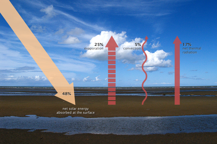
For the energy budget at Earth’s surface to balance (globally and annually averaged), processes on the ground must get rid of the solar energy that the ocean and land surfaces absorb. Energy leaves the surface through three processes: evaporation, convection, and emission of thermal infrared energy.
Edim wrote, “His “total radiation absorbed by the surface (sum of the net solar radiation at the surface and the downwelling longwave radiation at the surface)” does not make any physical sense… Downwelling lw does not power anything. The only energy input (ignoring geothermal) at the surface is the absorbed solar radiation.”
Wrong. That’s the “skydragon slayer” fallacy.
Downwelling longwave radiation is real, and measurable. Of course it increases temperatures at the surface.
When soil or water absorb radiation they don’t know or care whether that radiation was emitted by the Sun or by radiatively active gases in the air. Either way, absorbing that radiation makes the soil or water warmer than it otherwise would have been.
Stay away from PSI’s web site, and their idiotic “skydragon” book, unless you like being confused.
I am never going to understand this….
“because the entire Arctic Ocean is getting advected energy in the form of warm water moved up from the Pacific.”
through that little bitty gap….Bering Strait
…when the other side is wide open…and the Atlantic flows directly into it
I think someone needs to stick a thermometer in the Atlantic..
I assumed he meant both Pacific & Atlantic Oceans.
Latitude
From the Nautilus journeys under the Arctic sea ice, the Arctic Ocean at the pole is 13,410 feet deep. Five times larger (in area) than the Mediterranean Sea. Larger than the Gulf of Mexico. Hudson Bay. Baltic Ocean. That’s a lot of water to “heat up” with only the current coming north between Alaska and Russia-Siberia through the Bering Strait. The rivers dumping (fresh) water north from Siberia and Canada are cold in summer, frozen over solid in winter. They are large rivers, but not much “heating energy”.
But is is even worse than that: The Bering Strait is several hundred miles (200 + kilometers) long, so its “resistance” to water flow is much, much greater than the very narrow, much shorter, very deep orifice of the Mediterranean straits at Gibraltar. And the Bering Strait is very shallow!
Lots of heat reaches the Arctic Ocean as depicted on these graphics via both the Thermohaline Circulation and the Gulf Stream
But that heat does not come from the Alaska-Siberia side!
RACookPE1978 – June 14, 2019 at 5:42 pm
RAC, …… that doesn’t make no never mind difference any which way, …… because, to wit:
Quoting the author, … and citing his Figure 2 graphic, …..to wit:
RACookPE1978 – June 14, 2019 at 5:42 pm
Quoting the author, … and citing his Figure 2 graphic, …..to wit:
And, as I intended to point out, that tiny area available for actual water flow from the isolated Bering Strait far away from the greater Japanese current hundreds of kilometers south of the strait is NOT large enough for enough “hot” water to flow through to affect the Arctic Ocean.
Now, if the original author wants to make the claim about “total energy coming from the mid-Pacific north” in the form of air currents and hot (warmer, wetter, more humid) air to the entire “Arctic as a whole of land, mountains, the Arctic Ocean itself and tundra” then I would listen. May not be convinced since the original author has to show that movement of surface winds and storms and air masses.
But the Arctic Ocean itself? No. Not enough water has been measured actually flowing through the Bering Strait for “hot water masses” to be significantly affecting Arctic Ocean heat balances.
Not sure why this continues to be argued — obviously large amounts of “heat” enter the Arctic via the Atlantic — Willis simply left out “Atlantic”. Trust your common sense — that’s why open water extends well north into the Arctic on the Atlantic side.
nope..you don’t “leave out” the Atlantic…and mention the Pacific
….if anything…it would be the other way around
Absolutely. Only the Atlantic circulation matters when you consider water-borne heat flow. That said, somebody must predict, then confirm, the assumption that Siberian and Canadian river flow is also negligible. Easy to assume, easy to say, easy to claim, harder to quantify.
“But that heat does not come from the Alaska-Siberia side!”
And not from the north side of the Indian Ocean, either.
Now I could be confused at interpreting the authors words, so let me try this again, to wit:
Quoting the author (Willis E), …..… and citing his Figure 2 graphic, …..to wit:
Willis explicitly stated that “the strongest energy exportis from the tropical Pacific”, …… which was correct because the tropical Pacific is a lot warmer than the tropical Atlantic.
And then Willis states that “And on the other hand, the most energy is imported into the Arctic ”, ….. meaning not into Antarctica. Now I could be wrong but I ASSUMED a paragraph “break” between the 1st and 2nd sentence which would have divorced the 1st claim from the 2nd claim thus HOPEFULLY negating any confusion.
And then Willis states that “the entire Arctic Ocean is getting advected energy in the form of warm water moved up from the tropics”. From the TROPICS, not the tropical Pacific.
To illustrate:
The Bering Strait is only 82 km across total from shore to shore, with relatively “sharp” drops from shore side to the flat Bering Sea bottom.
The US side of the three passages – between Cape Prince of Wales and Little Diomede Island is a generally uniform 40-45 meters deep, with a very small “channel” 50 meters deep right in the middle. (Only a few hundred meters across.)
The short gap between Little Diomede Island (US) and Big Diomede Island (Palin’s ‘You can see Russia from my state’ comment) is only 6 to 17 fathoms deep, but only a few km across.
The “larger” gap between Big Diomede Island (Russia) and the Siberia coast is less thoroughly surveyed on US maps – at least on unclassified US maps! – but averages 20 fathoms (25-30 meters) deep with three “hills” underwater only 40-60 feet below the water.
1 fathom = 6 foot = 1.8288 meters.
Recent current measurements show the “modeled” volume of water crossing through the Bering Strait is much lower than the computer predicted model flow, with measured currents 10 meters above the bottom only 35 cm/sec.
.68 knots.
.35 meters/sec
1.26 km/hr, or 1/4 of a walking pace.
Thank you. I have looked at the strait but wasn’t aware just how little flow there was. Seems that there may be a net flow into the northern Pacific IIRC.
No, the numbers I’ve seen show an irregular flow north through the Bering Strait. It does goes up an down, and has a high std deviation (it varies quire a bit from the average flow) but doesn’t appear to go “negative” or flow south.
But, at only 0.35 m/sec, it isn’t flowing very fast either compared to many ocean currents 4 to 10 times quicker.
Many times more volume goes through the Davis Strait and Fram strait towards the Atlantic Ocean. See https://journals.ametsoc.org/doi/full/10.1175/2010JPO4536.1 for example.
Area comparison.
Davis Strait. 300 km wide x 1500 meters (1.5 km) deep = 450 km square.
Bering Strait. 78 km (82 km total -islands) x 40 meters (0.040 km) deep = 3.12 sq km in area.
There is a teleconnected linkage between El Nino episodes and roughly 8 month lagged major warm pulses to the AMO. E.g. in August 1998, August 2010, August 2016:
https://www.esrl.noaa.gov/psd/data/correlation/amon.us.data
I was stopped cold in reviewing this post by the word “niggling”:
“Niggling – a persistent annoyance”
I got to wondering about what the IPCC official scientific definition of this word is, since they love using terms like “High Confidence” instead of 90% confidence.
“Niggling – the inertial space-time event of adjusting a measurement or set of non-overlapping measurements to be within one standard deviation of an expected trend line as demonstrated by a pseudo-substantial predetermined non-relational computer model of the process being analyzed.”
Now I am niggling about whether the people within the IPCC ever stop niggling?
I love obscure words, the English language is a constant marvel.
w.
Willis Eschenbach “I love obscure words”
defenestration
And why do you suppose the English language needs this word?
Because sometimes, people need to be thrown out a window…
Defenestration – RP Lister
I once had the honour of meeting a philosopher called McIndoe
Who had once had the honour of being flung out of an upstairs window.
During his flight, he said, he commenced an interesting train of speculation
On why there happened to be such a word as defenestration.
There is not, he said, a special word for being rolled down a roof into a gutter;
There is no verb to describe the action of beating a man to death with a putter;
No adjective exists to qualify a man bound to the buffer of the 12.10 to Ealing,
No abstract noun to mollify a man hung upside down by his ankles from the ceiling.
Why, then, of all the possible offences so distressing to humanitarians,
Should this one alone have caught the attention of the verbarians?
I concluded (said McIndoe) that the incidence of logodaedaly was purely adventitious.
About a thirtieth of a second later, I landed in a bush that my great-aunt brought back from Mauritius.
I am aware (he said) that defenestration is not limited to the flinging of men through the window.
On this occasion, however, it was so limited, the object defenestrated being I, the philosopher, McIndoe.
It is an important word for those who study Czech history.
defenestration – great sports with medivial religious herolds diplomacy:
https://www.google.com/search?client=ms-android-huawei&ei=0gcFXeWnJ4HJrgSctICYAg&q=defenestration+of+Prague+meaning&oq=defenestration+of+Prague+meaning&gs_l=mobile-gws-wiz-serp.
“Niggling”? Obscure? Have you ever been to Australia, you niggling bastard?! 🙂
Bit of niggle in the front row . .?
So, is it possible to look at the time versus temperature record along your line of zero net advection energy transport what do we see?
Interesting thought …
w.
Without considering emissivity the rad/temp relationship is junk.
A surface LWIR of 500 w/m^2 is as bogus as cold fusion and for much the same reason.
500W is the sum of SW + LW. And the value is a real measurement for a change. 😄
Agree, emissivity is critical, so too is intensity, for energy to be thenalised and measured as temperature. Moonbeams can’t give you a suntan. 1360W at TOA contains. Broad spectrum of energy frequencies. IR is a weak fraction of that and the quantities are not additive properties. Its like saying two objects at 20C will make an object in the middle 40C. Nup.
Funny that you should mention Moonbeams. It atually gets warmer at full moon.
https://asu.pure.elsevier.com/en/publications/lunar-influence-on-diurnal-temperature-range
Don’t knock cold fusion. You can see it actually happen here:
https://youtu.be/OOcWAcecPxE
If an energy source can’t cook dinner it’s not science.
Watch the video. The gas flame is only warm as he passes his hand through it. But it melts titanium, and vaporises tungsten. Moreover it does so way below their melting point with them glowing white. A copper coin is later subjected to the flame until it glows white but it is not hot enough to melt through Teflon. The coin is instead distorted by the Teflon. In an earlier bit some carbon on the Teflon reacts with the titanium when it too is glowing white and pressed against the Teflon causing what is apparently a fusion reaction.
Something glowing white should be a lot hotter than 400 degrees C. Clearly there is something very weird going on here. The inventor refuses to believe his eyes or the instruments giving the temperature. This leads to quite a confrontation. So LENR might not boil your hand or cook your dinner but it can vaporise tungsten. This is a new kind of fire.
Watch the video. If this kind of tech did turn out to be usable it would probably upset the AGW lobby even more than the oil industry, as it would rob them of their justification for telling everyone what they could do.
Let me know when such can generate compelling evidence of a continuous flux of neutron emissions on demand from this active ‘fusion’ source. No neutrons, no cigar.
Very uncontrolled experimentation, amazing for Engineers and Scientists.
Obviously this has major uses where low temperature cutting is desirable.
No neutrons, no fusion. Exactly. If our Sun for example received its heat from fusion, we would all be dead from radiation. Minimum gamma rays (neutrons) would need to be a factor of three more than we are currently receiving.
If I had to guess at what is happening in the video, A hydrogen catalyst induced chemical reaction on a atomic scale during a plasma state. Transmuting the metals. (It is said that browns gas when applied to iron, Will saturate it with hydrogen so that it does not rust)
My sister makes gold jewelry with the water torch commercially available.
Willis …. great post. But I have a concern. In your previous post you note …. 3.7W/m2 is what is “expected “ from a doubling of CO2. Question, is this a real measurement, or … is the total radiation absorbed just a calculated figure based on what is “expected” based on models?
“… is this a real measurement?”
How could it be measured? The concentration of CO2 has not doubled.
It is a calculation, based on a simple logarithmic growth model, with a ‘fudge_factor’:
3.708=fudge_factor*ln(2)
where fudge_factor=5.35 was proposed (for use by IPCC) by Gunnar Myhre et al. in 1998:
“MYHRE ET AL.: RADIATIVE FORCING DUE TO WELL MIXED GREENHOUSE GASES ”
https://agupubs.onlinelibrary.wiley.com/doi/pdf/10.1029/98GL01908 [pg 2718]
Hmm. It’s a bit more robust than a “fudge factor”. The alpha parameter is determined from the log forcing curve.
The 5.35 from Myhre et al (1998), “Radiative Forcing due to Well-mixed Greenhouse Gases” is from Table 3., captioned “Simplified expressions used in IPCC[1990] Table 2.2”.
In fact go back a little to section 3 of Myhre et al and Table 1, which deals with clear sky radiation and we find “For CO2 the agreement between all three models is very good”. Models LBL, NBM and BBM give 1.759, 1.790 and 1.800 (all W/sq km). Table 2 shows “Global-Mean Adjusted Cloudy Sky Radiative Forcing” and for CO2 gives 1.370, 1.313 and 1.322.
Yes, they are different to what Willis says but … and here’s the important point … they were derived using THREE MODELS rather than empirical evidence. Model LBL is from Myhre & Stordal [1997], the NBM model is from Shine [1991] and the BBM model is from Myhre & Stordal [1997].
All three models are by authors of Myrhe at al (1998) and they are somehow accepted as gospel?
The LBL models are engineering models.
sorry. tested and validated. used in weapons design
here
https://www.nature.com/articles/nature14240
You, perhaps, need to understand that the Myhre et al estimate for the alpha constant does not in any way contradict Willis’ observations (or vice versa). Myhre simply provides a formula for calculating the TOA forcing for different ghg concentrations (5.35 for CO2). The climate sensitivity (i.e. temperature change) due to the forcing is a separate argument.
Willis found a relatively low sensitivity. There are 2 reasons which, at least, partly explain this:
1. The 3.7 w/m2 forcing cited is for the Top of the Atmosphere (TOA) – not the surface. A forcing of 3.7 w/m2 at the TOA should result in an increase of ~6 w/m2 at the surface.
2. Looking at the surface energy absorption values, Willis’ observations appear to be concentrated on a similar (same?) line of latitude. I suspect this is not representative of the global surface energy. The problem here is that it’s not possible to use a direct linear relationship between Energy and Temperature. Energy varies in proportion to the 4th power of temperature.
Basically the temperature change for a 3.7 w/m2 forcing will be smaller at 500 w/m2 than at 390 w/m2
Re: John Finn June 15, 2019 at 4:11 am
Ignore reason 2 in my previous post. I think Willis is using global averages. The surface energy values also include energy lost through convection and evaporation so not all of the ~500 w/m2 is realised in the surface temperature.
My fault – I read the article too quickly. My other points are still valid though.
I would say it’s a calculation based on physics.
After that it’s all about the feedbacks and, as CM so eloquently pointed out, the feedbacks are grossly miscalculated.
And if Happer is right, and the wings of the Voigt profile must be suppressed to match the measurements, then this forcing could be as low as 2.6W/m². Then, combining this result with the Willi’s one, ECS could be as low as 0.27K.
https://ams.confex.com/ams/15CLOUD15ATRAD/webprogram/Handout/Paper342816/AMSVancouver2018poster.pdf
Spectral line broadening is a thing. link It is most pronounced in the lower atmosphere where absorption by water vapor predominates. It’s also less important in that case because the main absorption band of CO2 overlaps with that of water. In the upper atmosphere, spectral broadening is much less pronounced.
Willis, I posted on your other article, but I’ll say it again in case you missed it.
http://oceans.mit.edu/news/featured-stories/missing-peice-climate-puzzle.html
If you correlate surface SW upwelling to log CO2, you’ll find a close to 3.7 W/m^2 relationship (I got around 4). When correlated to temperature, I got about a 1.6°C increase in Berkeley Earth or 1.3°C for HadCRUT for each decline of 3.7 W/m^2 in CERES SW upwelling radiation.
I used CERES EBAF Ed 4.1 and the “gsfc_sw_up_all_mon” variable. My calculations might be slightly off, so YMMV, but give it a try and see what you get.
Here is my correlation of CERES Surface SW Up to two temperature data sets (Berkeley and HadCRUT):
Berkeley Earth is a better fit. It implies a 1.6°C increase for each 3.7 W/m^2 decrease in surface SW up.
Here is a second correlation of log CO2 to CERES Surface SW Up, showing that for each doubling, the radiation changes by about 4 W/m^2 (close to the presumed 3.7 W/m^2).
My last look at the terrestrial energy budget was Graeme Stephen’s review paper of a few years ago.
As I recall he reported the surface energy budget to be known to only ±17 W/m^2 accuracy. Does that do anything to the uncertainty in your data, Willis?
Pat, I’m not sure which surface energy budget Stephens used. I used the CERES EBAF dataset. The precision of that dataset is much better than the accuracy.
My best to you,
w.
Pat,
So pleased to see your reminders that a proper calculation and reporting of errors is. in much of hard science, routinely expected, often useful and sometimes critical.
One of the hallmarks of climate studies is the comparative absence of proper and conventional error analysis. In my view, this is a major factor that allows the adjective “poor” to be added to “quality” when describing climate science overall. I compare it to the current calling out of some news as “fake” news as prior standards of accurate reporting have been avoided.
I note that some climate researchers do make an excellent job of proper error analysis. Their positive effort is denigrated by colleagues who know little about this essential topic. The good guys need to call them out for non- compliance with legislated requirements to follow prescribed paths in reporting error and uncertainty, where such paths exist in the countries concerned. Geoff
Thanks, Geoff, and I long to see that day. 🙂
Good to see your post, and hope you’re relatively pleased with the recent Ozzie elections.
Great comment. I suspect that in many cases the error component is larger than the stated value which makes the scientist look stupid. Consequently, ignoring errors means your conclusions look accurate, at the expense of ethical science.
Exactly on point, Jim. All of consensus climatology fails in exactly that way.
Major inaccuracies are ignored in all branches – climate modeling, the air temperature record, and in paleo-temperature reconstructions.
The entire field is no more than an exercise in false precision.
‘All and Sundry’ is an olde English mnemonic similar to the musical one ‘every good boy deserves fruit’ EGBDF, which are the lines on the treble clef.
All and sundry was first used, according to scrolls found in Glastonbury, by a monk, Willis Scarlett who also did some odd jobs for the famous Robin of Loxley.
Scarlett was interested in the radiation budget of the sherriff of Nottingham and used the formulae A + I + Hu
Where a is All of the downwelling , I is the irradiance due to angular plane and Hu the humidity or dryness.
‘All and sundry’ was a good for Willis Scarlett to remember it
“All and sundry”
Sundry is derived from a very old English word “syndrig”, meaning private or separate.
So the phrase means all collectively and each separately or privately.
However, in today’s bifurcated political world, the phrase could just as well mean “All (meaning those who agree with us and therefore have standing) and sundry (those who disagree and should therefore be treated as separate and worthy of dismissal, i.e. the “deplorables”)!
So thank you Willis for being so inclusive!
Thanks for the nice etymologipolitical explanation, I laughed out loud.
w.
Great article!
Per Joe Bastardi: El Nino is also a massive water vapor pump, pushing large volumes of water vapor into the atmosphere. Especially noticeable where it causes increasing water vapor in dry environments.
Keep in mind that in other locations it’s La-Nina that becomes the “water vapor pump”. It all just depends on where the warmest water is located at the surface. In La Nina the hot water is in the Western Pacific and we get the moisture hit in Australia, but severe droughts and a heat pulse during El-Nino. The water precipitates out closest to the hottest surface waters. But the heat pulse goes everywhere within the tropics regardless (but then again the lack of rain and trade winds will do that).
Just a small point about the 3.7 w/m2 . This is a Top of the Atmosphere (TOA) forcing. My understanding is that the surface forcing will be greater. To illustrate consider the following approximate energy flows.
Solar Energy In = LW Energy out (to space) = ~240 w/m2
Surface Energy UP = ~390 w/m2
Reduced Energy output due to 2xCO2 = ~4 w/m2
New LW Energy out (to space) = ~236 w/m2. But this results in an imbalance between incoming solar energy and outgoing LW energy so the earth’s surface and lower atmosphere will warm – until equilibrium is re-established (240 w/m2 -> out).
Emissivity (2xCO2) =~ 236/390 = 0.605
Surface Energy flux required = 240/0.605 = 396.6 w/m2
From Stefan-Boltzmann formula this implies a temperature increase of around 1.2 deg C at the surface.
I had suggested an alternative (simpler) method to derive this same second post result in a comment to the first post. That method also gives the relative significance of ENSO in the calculated warming trend by looking at the Enso Index coefficient. The method is generally called multivariate regression
Willis,
The Arctic receives more than the Antarctic because the…….
—————–
I think, this may be wrong…
Unless you can consider to check the amount of precipitation of Arctic versus Antarctic, and prove that Arctic receives more than Antarctic, then you still have to consider that basically you may be wrong with the above statement of yours…by not taking in account the “parameters” of energy transfer,
“Tension” and “Current intensity”, which from as far as I can tell seem to be different at some given degree point, in between Arctic and Antarctic.
Oh well, just saying,
just in case…
only trying a help…with no doubt of completely me missing the point here, 🙂
cheers
Willis, from your previous post:
“The total radiation is the sum of the net solar radiation at the surface and the downwelling longwave radiation at the surface.”
What is the physical meaning of this “total radiation”? I don’t see any. This is how it is usually defined:
Rn = Sn + Ln = Sn + Ldown – Lup
Rn is the net surface radiation. It represents the gain of energy by the surface from radiation.
Sn is the solar radiation absorbed by the surface or net solar irradiance of the surface.
Ln is the long-wave irradiance of the surface (Ldown – Lup).
You need to subtract the upwelling long-wave radiation from your sum to get the net surface radiation. But like I said, I don’t know what you mean by the “total radiation”, maybe something else. What does it represent?
http://www.met.reading.ac.uk/~swrhgnrj/teaching/MT23E/mt23e_notes.pdf
Edim, I’m looking at what is actually absorbed by the surface. I say that is downwelling longwave and downwelling solar after reflection. However, this didn’t include the import and export of advected energy energy.
That gives us to total influx to the surface.
Now, as you point out, this doesn’t include how the surface loses that energy to stay in steady-state. That is outgoing radiation plus sensible heat plus latent heat.
I’m not looking at that. I’m looking at incoming energy, what is available to heat up the surface.
w.
Willis,
A couple of thoughts to consider.
1. The speed of transport is much different between convective (atmospheric) and adjective (oteanic) heat transport because of the difference between wind speeds and ocean currents. Thus El Nino effects are seen in the atmosphere over a period of many months, while they are seen in ocean temperatures for many years (20 or more).
2. Ad’vection should vary linearly with the tropical ocean temperatures, whereas convention should vary exponentially. This is because convention is based on water evaporation. The partial pressure of water vapour varies exponentially with temperature. Thus not only does the amount energy transferred to the atmosphere by evaporation increase exponentially with temperature, but the convective driving force, driven by density differences of different air masses, is proportional to this exponentially increasing water vapour content.
dh-mtl, exactly! I fail to see how non linear physical response to said energy flux can produce a linear T flux change per doubling? It is just not logical.
CERES data tell us virtually nothing about near-surface advection. The zero-contour lines do not correspond at all to the well-known features of surface flows. They are nothing more than the location where planetary TOA emissions do not require anything beyond local radiative factors to infer intensity according to the theoretical “climate science” paradigm. That’s a far cry from actual geophysics.
I think a simple thought experiment might help visualize the effect of atmospheric pressure has on planetary temperature. If you heat a large potato and a small potato to 100 degrees, which one cools faster. This is very analogous to Venus, earth and Mars. Venus is very hot and has no diurnal temperature fluctuation while Mars is cool and has a vast temperature fluctuation between day and night. The earth fluctuation is about 8 degrees. Venus’ atmosphere is 93 times denser than earth’s and earth’s atmosphere is 100 time denser than Mars’. Scientists have come up with an empirical equation which predicts planetary temperature to within 2 degrees celsius based only on atmospheric temperature and distance from the sun. This equation obliterates the potential of earth’s temperature running amuck by increasing CO2 from 0.03% to 0.06%. Venus and Mars are both 95% CO2.
Agree, emissivity is critical, so too is intensity, for energy to be thermalised and measured as temperature. Moonbeams can’t give you a suntan. 1360W at TOA contains a broad spectrum of energy frequencies. IR is a weak fraction of that and the quantities are not additive properties. Its like saying two objects at 20C will make an object in the middle 40C. Nup.
Willis.
An interesting article, but you are ignoring winter and summer.
Have a look at these temperature maps.
https://agree-to-disagree.com/rats-north-summer-south-winter
https://agree-to-disagree.com/rats-north-winter-south-summer
Sheldon, these are yearly averages of anomalies. I’ve subtracted out the regular part of the seasons. What is left is when winter is warmer or colder than the usual average winter. I’m looking to see whether and how much the corresponding change in incoming energy was
Willis, maybe the explanation of the unchanged trend is that the advected waters mostly also simply emit most of their heat into the atmosphere for onward escape to space.
Thanks, Gary. The trend is unchanged whether we include advected data or not. And the increase in R^2 argues against the idea that the advected energy is not included in the surface measured temperature record.
Regards,
w.
Only because you ask sir,
Sundry as in “asunder” or separate; so “all and sundry” suggests “collectively and individually” or perhaps “jointly and severally”. Probably double counting in this context.
[But “all and sundry” also refers to how many diapers can fit on a standard clothes line in the backyard” .mod]
Thank you, sir.
w.
I’ve clarified in the head post (I hope) the question of the Arctic heating. Thanks to those who pointed it out.
w.
I’ve also added a comparison to the head post using HadCRUT temperature data in place of CERES data.
w.
Good stuff, Willis.
I’m very much looking forward to a resolution of how to distinguish the sundry from the all. Could we perhaps have a competition?
This could add an addition to the heat flux. I have used a lot of time to understand energy flux. E.g as a Finn I know that you get more snow when there is a lot water (moisture) on the Athmosphere, but it means that you have to have very warm somewhere over a Sea to get water from the Sea to high! Here in Nordics Golf Stream is feeding our ”snow machine”. The very same must be in the Greenland, the more ice there, the more snow and the more water in the Athmosphere over the Greenland.
Here is an intresting study you may get some more energy flow for your ”GETBE” (Global energy temperature balance of the Earth): https://www.nature.com/articles/s41467-018-05337-8
Willis , Can you explain to the great unwashed (of which I am a part of ) how your advection numbers are supposed to add up. The last time I checked total imports around the globe has to equal total exports, no matter whether it is beans or heat.
John Finn. I think you put your finger on an important point: “Just a small point about the 3.7 w/m2 . This is a Top of the Atmosphere (TOA) forcing. My understanding is that the surface forcing will be greater. ”
“From Stefan-Boltzmann formula this implies a temperature increase of around 1.2 deg C at the surface.”
It shows how easy it is to be misled by numbers, as many comments prove. I would like WE to look more at this, as he has the mathematic skills. He could compare the total surface absorption with TOA radiation (absorption).
I’d caution against too-facile a comparison of Mr. Eschenbach’s result with equilibrium-climate-sensitivity estimates. Notice that he was careful himself not to draw any conclusions.
Now, I don’t profess really to have grokked what effect the seasonal adjustment has. But let’s say it results in a valid representation of the system stimulus. And the data no doubt look significantly different from what I imagine. But what if the period of that stimulus’s predominant frequency component is one month?
Then Mr. Eschenbach’s 0.39 K for a doubled-concentration forcing level would imply an equilibrium climate sensitivity of 3.2 K if the system could be modeled as a single-pole low-pass filter whose time constant is something like 17 years.
Obviously, that’s a lot of ifs. But it goes to show that in the absence of a lot more information we are well advised to withhold judgment.
For the sake of society we must simplify the talk about climate change. Most people are so confused by the science that they opt for the safe side of the argument. We must make things relatable or the UN (and government) will be successful with their agenda.
It would be good if you could use a different colour for all years with el Nino?
Hi Willis,
The 3.7 W/m2 used by the IPCC is for the Top of the Atmosphere (TOA).
Aren’t you comparing apples with oranges by comparing the surface T changes with the TOA radiative change?
I remember an article I wrote about global dimming and brightening in which this discussion played a role. I will send you an email about it.
Cheers, Marcel