This is not a novel result, for example:
https://wattsupwiththat.com/2018/03/30/tools-to-spot-the-spots/
Nevertheless, this is a solid analysis and exercise in citizen science.~ctm
By: Leron Wells
During my early teenage years as an avid fan of the Space Program I was patiently waiting for NASA to get the Shuttle flying so hopefully they could boost Skylab from its decaying orbit. However, I was very disappointed as I am sure everyone was when it was announced that Skylab would renter the atmosphere sooner than expected and there was no hope of saving it. I became very curious about the 11 year solar cycle when it was announced that the reason Skylab deorbited sooner than the NASA engineers calculated was because of the increased drag associated with the expansion of Earths outer atmosphere caused by the very active Solar Cycle 21.
Now we fast forward 3 decades and much to my surprise I have yet to see any concrete evidence of any correlation of Earths atmospheric temperature with the 11-year solar cycle. There have been many attempts on various surface temperature records with no real positive signature of any meaningful evidence that I have seen, “IMHO”. As a geophysicist with over two decades of experience and having developed numerous spectral applications for finding Oil & Gas, I took it upon myself to see if there was a correlation in the Stratosphere, how hard could it be, right? After all we now have over 40 years of satellite data which should be more than enough data to detect an 11-year cycle.
With permission from RSS I downloaded the binary dataset for both the lower Troposphere and the lower Stratosphere and began writing an application to read and display the data. The RSS binary data has global coverage for every month ranging from December 1978 to February 2019, which equates to 483 months of data. I designed the application to sum the data along latitude bands for each month and to do all spectral analysis calculations and visualizations in the latitude vs. time space.

Figure 1 Lower Troposphere Latitude vs Time
Figure 1 shows the plot of the lower Troposphere of the latest dataset available from RSS as of February 2019. The application has volcano images positioned by their eruption dates for Mt. St Helens, El-Chichon and Mt. Pinatubo as well as the Enso markers for strong, moderate and weak El-Nino’s and La-Nina’s. Also, at the base of the plot is a graph of the sum of all latitudes for each month. It should be noted that this sum does not include any latitudinal weighting so the Global average will be somewhat different than the true global average temperature for the RSS dataset for the Lower Troposphere. The latitude vs time lower troposphere plot “Figure 1”, clearly shows the latitudinal effects of both the ENSO cycles as well as the short-term cooling caused by Pinatubo and El-Chichon.
The lower Stratosphere plot “Figure 2”, shows the rapid warming caused by the SO2 injected into the Stratosphere by both El-Chichon and Pinatubo. Again, the graph below the plot shows the summation for each month and represents the globally averaged anomaly temperature for the most recent RSS binary dataset as of February 2019 for the Lower Stratosphere.

Figure 2 Lower Stratosphere Latitude vs Time
With the latitude vs time plotting accomplished the next step was to take advantage of the latitude vs time space to compute the spectrum for each latitude and generate the same type of plot as the previous temperature plots, but with the main color plot being latitude vs cycle length in years. I used the binned Periodogram algorithm to compute the spectrum for each latitude and display the latitude vs cycle length plot. The color in the latitude plot represents the spectral energy converted to the base 10 logarithm or what we call in Geophysics as DB Down or Decibels from maximum amplitude. This was necessary to normalize each latitude color band to a relative value so that all the spectral features for each latitude and each month would be normalized to the color bar and show the latitudinal spectral features in a pseudo relative manner for the latitude vs cycle length plot.
The equation for the color plotted spectral data is defined as:
logAmplitude = 20 * Log10(currentAmplitude / maximumAmplitude)
The spectral displays have the actual solar cycle length annotated for cycles 21, 22 and 23 as a reference because the average solar cycle length is assumed to be 11, but the exact cycle length varies by some number of years for each cycle. The graph at the base of the cycle length plot is the average cycle energy for the entire dataset represented as a black line, the Northern Hemisphere mid latitudes as a red line and the Southern Hemisphere mid latitudes as a blue line. It should also be noted that the spectrum graph at the base of the plot is not utilizing the logarithmic amplitude, and it is plotted as the actual linear amplitude as spectral power taken directly from the binned Periodogram. This was chosen because the peak of each cycle for the various latitudinal bands are better represented by showing their relative strengths as a linear function.
Figure 3 shows the spectrum plot for the lower Troposphere in the latitude vs. cycle length in years display. There are many localized anomalies that one could spend quite some time speculating about what the source could be, but the very interesting and powerful 13.5-year cycle leads me to believe that it could possibly be associated with the solar cycle with a reactionary time delay. But never the less, there is no 11 year cycle that shows up in the Troposphere. Again, the black line on the lower graph represents the global average, the Red Line represents the middle latitudes of the Northern Hemisphere and the Blue line represents the average of the Southern Hemisphere mid latitudes.

Figure 3 Lower Troposphere Latitude vs Cycle Length (Years)
Figure 4 shows the latitude vs cycle length in years plotted for the lower Stratosphere and clearly shows a very strong 11 year cycle in the Southern Hemisphere and also shows a meandering cycle length in the Northern hemisphere that varies slightly by latitude from 10 to 10.5 years, but is very close to the period that fits within the range of the Solar Cycle lengths for the satellite date range.

Figure 4 Lower Stratosphere Latitude vs Cycle Length (Years)
Conclusion
The spectral methodologies that I have applied to both the Lower Stratosphere and Lower Troposphere RSS data are very robust methodologies and have served me well throughout my career finding cyclical patterns with much less data than what is available in the RSS monthly global satellite record. There was a concern that the effects of Pinatubo and El-Chichon was the cyclical pattern that I was seeing in the spectral display that correlated with the solar cycle period, so just to be sure I muted the period over the range that Pinatubo caused the stratospheric warming and reran the Spectral plot and the results were very similar for both the Stratosphere and the Troposphere.
All the code that generated this data and produced the plots was written from scratch in C# in the community edition Version of Visual Studio 2017, except for the binned Periodogram which I got from Numerical Recipes in C. The next step will be to use the Wiener Levinson algorithm to utilize Predictive Deconvolution to remove the cyclical patterns for each latitude band individually and display the deconvolved results to see the latitude vs Time space with all cyclical patterns removed, so stay tuned for the next iteration. Also, much appreciation to Remote Sensing Systems for providing access to the binary satellite data.
Leron T. Wells III
Can we get higher resolution links to the images/graphs ? Those images are too small to read.
Cheers !
Ditto
Yes, those plots are very detailed and unreadable at the that size. Please provide something legible, it is meaningless as it is.
Congratulations Leron on a fine bit of analysis. Most impressive.
It would be interesting to see if you get the same results from the satellite UAH data set by John Christy and Roy Spencer. They are the only temperature climate scientists that we skeptics trust.
Dr. Judith Curry deserves respect too.
She is not a “temperature climate scientists”. He did not say “only climate scientist”.
This article looks interesting. It would be good if he published his code.
Funny they adjust their data and dont supply the “before” (raw) or the codes that do the actual adjustments.
Would you like some cheese to go with that whine?
mebbe you could get a position created in your program where they could learn how to do it right.
what does it take to get such a position created?
They’re probably trying to hide their methods. You should file a FOIA request and see if they stonewall you for ten years.
If we are sceptics should we trust any of them?
Shouldn’t we treat all reports as suspect until shown otherwise?
The sunspot data follows distinct cyclic pattern with high autocorrelation and it can be modeled better by ARIMA. It shows 11 year cycles.
We have developed model equations for the sunspot time series data and the TSI time series data at the top of the atmosphere.
These are good models with R >0.9 values.
The model enables us to predict these solar cycles until 2030.
Not pointing at anyone in particular, but Trust and Respect are two different things. You can trust that a snake will try to bite, so you respect that threat and keep to a safe distance.
I reiterate, not I am not referencing anyone at all.
On the other hand, both respect and trust are earned not given.
SO2 from volcanos can cool the atmosphere. But SO2 is a common air pollutant that has been removed by clean air action. It started round 1980 and now we are at levels as low as round 1960s.
Could the effect of this be analysed?
That is exactly the problem: too many confounding variable. Volcanic temporal coincidence with SSN, similarity of 9y lunar and 11y solar, any long term trends like clean air act just get confounded with steady changes in CO2.
This is why it is impossible to attribute to anything definitive to CO2 if you are being honest and objective.
Pinatubo emitted 20 Megatons of SO2…and resulted in a 0.6 C temperature drop for a year.
http://volcano.oregonstate.edu/b
SO2 emissions peaked around 1980 at ~150 Megatons annually…currently down to 100 Megatons. Shouldn’t that 50 Megaton (2 and a half Pinatubos) produce a > 1.0 C “cooling reduction” (i.e. warming)?
https://ourworldindata.org/air-pollution
Sulfur particulates are in the climate models, and I would assume SO2 would be as well…so where is the discussion about the ~ 1 C warming since 1980 from our SO2 and Sulfur particulate abatement?
Also, do the SO2 levels and Particulates drop rapidly enough after only 1 year…or does the climate “readjust itself” responsive to the temperature drop?
Not the same — the volcanic SO2 that cools temps significantly is that which gets into the stratosphere. Pretty much zero human SO2 gets there, tho some have suggested human SO2 enhances cloud albedo (not proven).
And they try to tell us what the weather will be in 20 year plus time????
During periods of low solar activity, North America is threatened by frequent stratospheric intrusions. This is related to the blocking of the winter polar vortex in the lower stratosphere over eastern Siberia.
At present, the very strong blocking of the polar vortex is visible below Greenland. It will bring arctic air to Europe.
“During periods of low solar activity, North America is threatened by frequent stratospheric intrusions.”
Do you have a reference for this ren?
It is already evident that during the solar cycle minimum El Niño does not work in North America.
Stratospheric Intrusions are more common in the winter/spring months and are more frequent during La Nina periods.
https://www.cpc.ncep.noaa.gov/products/stratosphere/strat_int/
I can’t seem to find any link between Stratospheric Intrusions and periods of low solar activity. Am I missing something?
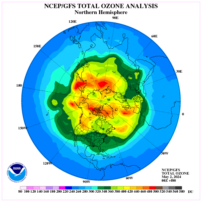
You do not follow the distribution of ozone during winter over the polar circle.
http://oi68.tinypic.com/2iayf74.jpg
There’s plenty of references for that. Karin Labitzke spent her entire career showing how solar activity affects stratospheric polar temperature and geopotential heigh. Look for her papers alone or with Harry van Loon. And seeing it is as simple as running the NCEP/NCAR reanalysis tool asking for the right months and years:
The weather of North America and Eurasia on certain winters is completely determined by solar activity.
Thank you.
“The weather of North America and Eurasia on certain winters is completely determined by solar activity.”
No it’s not.
Solar UV intensity is just one influence of many.
Else we could completely predict the outcome of solar min NH winters.
We cant.
Vis this year when a continental easterly never made it to the UK when models predicted it was likely.
The in-place westerly QBO could have been the reason it didn’t by failing to deflect planetary waves sufficiently pole-ward once the SSW event occurred.
We are talking weather here in terms of a hemispheric season and chaos reigns
If a cyclic, peak-to-peak change of about 1W/m2 every 11 years hits the top of the Earth (a definite and clear repetitive input signal), but can’t be detected in the surface temperature record (an output signal), what should be made of the climate scientist’s assertions that they can detect a clear signal from man-made CO2 increases, which has only caused a non-repeating increase of 1.68 W/m2 since 1750, as estimated by the IPCC?
Let’s put it another way: if the Earth’s climate system takes a repetitive signal of “1” with a period of 11 years at its input, and no detectable changes can be discerned at an output (say surface temperature or precipitation or whatever) as a result of that cycle, which has gone on and on for centuries, I don’t see how it is possible that the output from that same system can be used to detect a ramp function at it’s input so minuscule that it takes well over a century (about 13-14 cycles worth) to hit the same peak-to-peak amplitude as the 11-year signal.
Even if you were one to accept that the solar input has to be cut into a quarter due to the day-night cycle and the spherical shape of the Earth’s surface (and I am not one to blindly accept that), you’re still comparing an identical amplitude for about 30 years of your non-repeating ramp function to 11 years of your repeating sinusoidal function. That sinusoidal function should be detectable far more easily than the ramp function. Yet the climate scientists claim not only that they have detected “fingerprints” of man-made warming in the temperature record, but claim to be able to have measured it.
What nonsense.
4 pi r2 and pi r2 is simple geometry, what part are you questioning?
Systems are driven by differences across their inputs: differences in voltage across a wire drives the current through it, differences in pressure drive water through a pipe. It’s not just a question of how much energy you throw into a system, as I can push both sides of a revolving door equally, as hard as I like, and it does nothing.
So when the sun shines full bore on the equator on a sunny day, but is filtered through clouds at 45 degrees north, that difference is what drives the phenomena we use to measure both weather and climate, as the heat is forced to move around due to spatial differential in input. The same with the day-night cycle. So when you just average out those differences by dividing in two, to account for the diurnal cycle and do it again for the cosine effect, you are eliminating the essential part of what drives changes in weather and hence climate variability.
Kurt, I have an analogy to support your point.
If you have a thermoelectric generator, it has a hot side input of say, 240 C max. If one installs such a device on a hot stove to operate a fan, the average temperature of the hot side is important. However knowing the average is not helpful if one wants to know what the performance really is at any given time.
For example if the average is 200 C and the peak its 300 C, then the device will cease to operate (permanently) once the limit of 240 is exceeded.
Similarly, when there is heating in the daytime at the equator of 1200 W/m^2 and zero at the poles, the behaviour of the atmosphere is not driven by the “average” input.
For example the heating of the air by the ground during the daytime in the tropics is massive, while at night it is reversed. Convection of heat into the air during the day produces phenomena that do not appear in models which have the average temperature applied to the whole surface.
Imagine an alternative Earth where solar flux somehow gets distributed around the surface of the Earth, to be spatially uniform at 1/4 of its current value, (without interfering with the Earth’s ability to radiate away its own heat) so that the only spatial and temporal variations in surface absorption could come from albedo variations. Ask yourself whether, in spite of the fact that the average daily, annual etc. amount of solar energy absorbed at the surface is exactly equal to what is absorbed by the real Earth, that nonetheless this hypothetical Earth would have a climate that behaves vastly differently than does the real climate, and if so, how?
My intuition, and I’ll admit that it is only that, tells me that the system where a spherical Earth gets its energy by rotating in an energy field coming from a single direction is going to cause the climate to behave much more erratically than if the same net amount of energy were coming inward from all directions at once such that there was no day/night cycle and every spot on Earth receives the same downward flux. And that the resulting climate from the rotating sphere system would not only never be in equilibrium even with a constant average daily input, but that it would exhibit very long term, unpredictable natural changes in climate, extending over many decades or even centuries, merely as a result of how the system is set up and having nothing to do with changes in solar output, or CO2, etc.
In that kind of a real world system, trying to measure or detect changes in climate attributable to changes in input flux that are very small in relation to the amount of total flux, and and very gradual (dare I say glacial) in relation to the rotational period of the Earth, is silly. And trying to simplify the system by removing its rotation and shape to try to tease out those changes is even sillier.
Very nicely put Kurt, thx.
The 800 year lag between temperature and CO2 raises the suspicion that it is an important factor and that the oceans are involved. It’s been 400 years since the little ice age and we seem to have reached an elevated plateau in temperature.
Kurt,
There is a huge difference between a periodic signal and a ramp.
Suppose I deposited 1 dollar in your bank account one week and then
took it out again the next week. After 10 years how much extra money would you have? Now suppose I deposited 1c a week in your account every week and again after a decade how much extra money would you have?
I agree there is a difference – that was my whole point.
If someone regularly deposits say $1,000 in my bank account every Monday and takes it out the next Thursday, I’m going to notice that pattern really quickly just from occasionally watching my bank balance, and wonder what’s going on – even with a lot of noise from my automatic deposits from my job, my mortgage payments, my credit card payments, and so forth. But if someone deposits $10 a week in my bank account, and all I’m doing is occasionally watching the balance, it would take me a much longer time to notice those payments given the natural fluctuations of the balance as paychecks are deposited, bills are paid, money withdrawn from ATM’s etc.
Yeah, my dad and I have the same name, and we used the same bank back when I was in the army during the Vietnam war. We lived on my wife’s income while overseas, so I had my monthly paycheck go directly to my bank account, (or so I thought). When we came back to the states, we wondered why there was only just around a hundred dollars in my bank account. My mom had noticed the increase in income, but just thought that dad was making more money than usual. (They did reimburse us.)
Could you provide a more scientific description of what you did ? What is “muting” , what exactly was the period you “muted”. Why did you not mute El Chichon with had a very similar effect on TLS?
How much of the 40y data set remains after the “muting”. I would say that almost 10y was affected by both events ( this initial upwards bump and the following persistent 0.5 deg C drop in TLS ) , if you remove the effects of volcanoes you have about 25 of a broken up dataset. That is not enough to detect the cycles. If you have not cropped out that much data, you are still looking at volcanic effects, which are being confounded with solar.
https://climategrog.wordpress.com/uah_tls_365d/
Also with your periods being a binary submultiple of the length of the dataset there is a strong possibility that you are aliasing the length of the record. What, if any, measures did you take to protect against that?
I suspect that your method may not be a “robust” as you think it is. Indeed that is one of trigger words for non scientific confidence in one’s methods.
It is a shame the Leron Wells has not taken the time or interest in his own article to respond to comments.
I guess when you are convinced of your own robustness, there is not need.
Greg,
Sorry about the late response, I had a number of software issues that required day and night dedication.
I appreciate your interest and concern about aliasing, however I do not agree with it in this scenario. Temporal aliasing is generally associated with attempts and discerning high frequency information in a signal that does not have fine enough sampling interval to represent enough data points of the signal in question. For instance JPEG generally has artifacts around text which creates spurious noise bursts, but the low frequency components of the characters make them easily visible.
The mute I did of the Pinatubo effects are not very scientific, I essentially starting point of the Pinatubo effects constant across the duration.
Here is the muted data that went into the Periodogram:
https://postimg.cc/2bGwCF7m
Here is the Spectral results of the muted Stratosphere data
https://postimg.cc/2qsp4Ys3
Now this is a highly disruptive and quick and dirty approach which suffers from Gibbs Phenomena but I had to do something to ease my mind.
Since we have detailed , gridded data for TLS and daily solar SSN , it may be better to look for direct correlation rather than periodic analysis of a rather variable cycle.
The solar cycle is much more easily detectable in the mid and upper-Stratospheric data.
The effects of solar magnetic activity on “climate” (temperature) of stratosphere and above is well known. Below tropopause, no compelling evidence exists.
https://wattsupwiththat.com/2019/02/23/study-a-solar-signature-in-many-climate-indices/#comment-2639290
Look at the subsurface temperature at the Equatorial Pacific.
http://www.bom.gov.au/climate/enso/wrap-up/archive/20190402.sub_surface_anom.png?popup
Here’s the current one.
http://www.bom.gov.au/archive/oceanography/ocean_anals/IDYOC007/IDYOC007.201904.gif
Thank you.
Many years ago I read a book “The Jupiter effect”. It stated that
approx. every 11 years the planets in the solar system all lined up, and the combined gravitation effect pulled on the Sun, causing changes in the sunspots and solar wind. .
Is this still the accepted reason for the 11 year cycle, if not then just what causes it.
MJE VK5ELL
Michael: “The Jupiter effect”
I was curious why the sun would have a ‘geocentric’ cycle, the length of Earth’s year seems like an arbitrary time period to measure a solar cycle. I was curious what the length of a year on other planets is (shown in Earth’s years):
Mercury .24 years
Venus .62 years
Earth 1 year
Mars 1.88 years
Jupiter 11.86 years
Saturn 29.46 years
Uranus 84.01 years
Neptune 164.79 years
Pluto 248.59 years
Your reference to Jupiter seems apropos.
claims of planets “lining up” tend to be astrological ( ie plus or minus 30 degree “conjunctions” ) rather than astronomically true alignments.
If astrologists find three or more planets within their eyeball range on one night, they seem to think it is an omen of some sort. I doubt the sun is impressed.
(1) I debunked “The Jupiter Effect” (by Gribbin and Plageman) in an article published in the journal “Icarus” of October 1975.
(2) How can the planets all line up every 11 years, when the heliocentric conjunctions of Uranus-Neptune occur at intervals of about 172 years? The last two took place in 1821 and 1993, and the next one will take place in 2164.
nasa? were saying Indias shooting that sat the other day was bad bad naughty as the reduced mag field in a low solar cycle meant it would make a mess of debris but bits also went higher and risk damaging space station
i dunno def not my specialty, the colours look pretty though;-)
uh…you might want to switch to a less potent smoke. Or maybe type AFTER you wake up and have had a cup of coffee? Lol!
the colours wouldn’t look as pretty ….
Maybe the post in question needs the Rosetta Stone or a cryptex (wiki “Da Vinci Code”) for interpretation?
If I’m reading this right, the southern hemisphere (with more water) is closer to the periodic solar cycle at 10 years than the northern hemisphere at 13 years…
There is obviously not enough data to really determine what is going on, but is it possible that the actual actions are some type of constructive/destructive wave mechanism, where the south is absorbing heat more, pumping that heat north over a time based on the amount of heat….so more heat absorbed takes longer to move north.
If that was the case, the strength of the solar cycle would also need to be taken in to account some how, and correlate that to the period of the temperatures.
Not sure if I am explaining that in a way that makes sense, but think of a pump pumping hot water in to a pool at some interval. If the temperature of the water being pumped changes, the pool temperature will change eventually, but not necessarily be in synch with the pump.
Just my thoughts,
Roland
This article of mine refers to solar induced changes in the stratosphere altering the gradient of tropopause height between equator and poles so as to alter cloudiness and the amount of solar energy entering the oceans:
http://joannenova.com.au/2015/01/is-the-sun-driving-ozone-and-changing-the-climate/
which fits the above findings nicely.
Appears to me that just the change in height would affect the amount of radiation from the Sun that is intercepted by the larger/smaller “sphere” and would also increase/decrease length of time the atmosphere is intercepting radiation as more of the atmosphere is in the path of the sun light longer or less of the atmosphere is in the sunlight for a shorter period each day. This would be apparent in the fact that the observed sunrise/set would also be affected by the thicker/thinner height of the atmosphere. And this would affect many other aspects of the way the globe is affected by the Sun.
This is a commendable job of demonstrating the very different responses of the lower troposphere and lower stratosphere to volcanic events and to solar variability. It would be nice to have the author clarify the precise mathematical nature of his “binned periodograms,” which one presumes involves some decimation (in frequency or time) of raw periodograms. The latter provide notoriously inadequate estimates of power density from short, non-periodic records (see: http://adsabs.harvard.edu/full/1993MNRAS.261..612P). Such clarification might also stifle the peremptory demands for “code” made here by the usual suspects.
Since the given link apparently stopped working, one might try finding:
Title: Improved Methods for Power Spectrum Modelling of Red Noise
Authors: Papadakis, I. E. & Lawrence, A.
Journal: Monthly Notices of the Royal Astronomical Society, Vol. 261, NO. 3/APR1, P. 612, 1993.
Is your ‘conclusion’ actually a conclusion?
I want to subscribe to your blog in order to receive blog posts via email.
Thank you. Love the length,breadth and heighth of your articles.