How does the Sun drive climate change?
Guest Post by Javier
The dispute between scholars that favor a periodical interpretation of climate changes, mostly based on astronomical causes, and those that prefer non-periodical Earth-based explanations has a long tradition that can be traced to the catastrophism-uniformitarianism dispute and how the theory of ice ages (now termed glaciations) fitted in.
Prior to the scientific proposal of ice ages in 1834, most scholars that cared about the issue believed that the Earth had been progressively cooling from a hot start, as tropical fossils at high latitudes appeared to support. By 1860 scholars had been convinced by evidence that not one but several glaciations had taken place in the distant past. By then scientists trying to explain the cause of past glaciations were split in two. Those following Joseph Adhémar, who had already proposed orbital variations in 1842, and those following John Tyndall, who proposed that they were due to changes in GHGs (greenhouse gases) in 1859, particularly water vapor.
For a time, the anti-cyclical, pro-GHG camp had the advantage, after James Croll’s hypothesis was rejected, and Svante Arrhenius in 1894 proposed CO2 as the responsible GHG. But then, doubts about the CO2 effect and a new formulation of the cyclical astronomical hypothesis by Milankovitch appeared that fit popular geological reconstructions of past glaciations. This swung the field again.
By the late 1940’s Milankovitch theory was well established, particularly in Europe, but not so much in America where reconstruction of Laurentide ice-sheet changes did not match the theory very well. But in the 1950’s a new consensus formed. The GHG theory was reinforced by Suess, Revelle, and Keeling’s work, while carbon dating led to glacial reconstructions at odds with Milankovitch theory.
In the 1960’s and early 70’s Milankovitch theory was discredited with only a handful of followers left. The anti-cyclical, GHG explanation enjoyed wide consensus, but due to the cooling at the time, scholars believed other factors must be at play. Then disaster struck for the anti-cyclical camp. In 1976, Hays, Imbrie, and Shackleton, analyzing Indian Ocean benthic cores for the past 450,000 years and showed that glaciations followed some of Milankovitch frequencies within 5% error. A 140-year quest had ended, and the cyclical orbital supporters had won.
Of course, GHG supporters are bad players and did not accept the defeat graciously. Since it was soon discovered in ice cores that GHGs followed orbital changes (as they should), it was soon proposed (and accepted without evidence) that they were required to amplify the orbital changes and to maintain inter-hemispheric synchroneity. Trying to turn the defeat into a victory, they claim that the frequency is set by Milankovitch but a great deal of glacial-interglacial climate changes are due to GHG changes.
You would think that after showing that climate was cyclical and astronomically based, propositions that other astronomical phenomena (like lunar periodicities or solar variability periodicities), might affect climate would at least be given the benefit of doubt. But no. The anti-cyclical camp enjoys centennial beatings by the cyclical mavericks, so they are building up for the next one by flatly rejecting any significant climatic effect from periodical solar changes. Apparently, they are undeterred by the evidence showing most periods of low solar activity during the Holocene are associated with cooling and atmospheric circulation and precipitation changes, like the LIA. There are about 10 abrupt climate events (ACEs) associated with low solar activity during the Holocene. Some have names like the pre-boreal and boreal oscillations, or the 9.3 or 2.7 kyr events, showing that the most frequent cause for ACEs is prolonged low solar activity.
I have already shown some evidence for that in my previous articles:
Do-It-Yourself: The solar variability effect on climate
Do-It-Yourself: Solar variability effect on climate. Part II
I have also shown that ENSO is under solar control:
Solar minimum and ENSO prediction
Yet the anti-cyclical crowd (IPCC included) takes refuge in the bean-counting argument that solar variability is only 0.1% and therefore too small to produce much of a change. This only shows how narrowly focused their view of climate is. They think that Earth’s climate can be explained solely with terms of W/m2 and after all 0.1% is only 1.4 W/m2 over the 11-yr cycle (solar irradiation), adjusted to only 0.34 W/m2 annual average insolation change at top-of-the-atmosphere (TOA) at 1 AU. However, the Earth received the same TOA insolation during the Last Glacial Maximum as now, so climate is clearly not a case of bean-counting Watts.
Today I am going to show you how solar variability affects Earth’s rotation speed, and why it is important. This issue was raised several times in 2010, but it is not understood by most:
https://wattsupwiththat.com/2010/10/03/length-of-day-correlated-to-cosmic-rays-and-sunspots/
Changes in the rotation speed of the Earth are measured as variations in the length of day (ΔLOD) defined as the difference between the astronomically determined duration of the day and 86,400 Standard International (SI) seconds. ΔLOD has been measured daily down to a 20 microsecond (µs) precision by interferometry since 1962. Annual changes at 1 millisecond (ms) precision have been reconstructed for the telescope era from astronomical observations. Variations in ΔLOD on annual and seasonal (semi-annual) time scales are highly correlated with angular momentum fluctuations within the atmosphere, mainly due to changes in zonal winds. The averaged annual and semi-annual oscillations in ΔLOD feature almost equal amplitudes of approximately 0.36 ms.
The semi-annual oscillation in ΔLOD has the following characteristics:
From November to January the Earth accelerates to ~ 0.2 ms-day (ΔLOD changes by -0.2 ms). Then it decelerates by nearly the same amount by April. Afterwards it accelerates to ~ 1 ms-day by July (ΔLOD change of -1 ms), before decelerating back to the initial value by the next November. The average amplitude is ~ 0.35 ms, but the NH winter component is much smaller than the SH winter component (see figure 1, inset).
This change is caused by the angular momentum of the atmosphere being higher in winter because the meridional circulation is much stronger during that season. This is the result of the winter pole receiving very little insolation as the Sun is above the opposite hemisphere. The dark pole becomes colder and the latitudinal temperature gradient steeper, and as a result more heat needs to be transported poleward, activating the meridional circulation in that hemisphere. The asymmetry of the NH (Northern Hemisphere) winter and SH (Southern Hemisphere) winter components of ΔLOD is due to the asymmetry in land masses between hemispheres having a strong effect on wind circulation.
Le Mouël et al., 2010 showed that the semi-annual component of ΔLOD responds to solar variability. This is an extremely important result highlighted only by a few skeptics and ignored by everybody else. Part of the problem is that the article’s method to show it is quite complicated, and most people did not understand the article or its implications. Let’s try a simpler way.
Let’s concentrate only on the NH winter acceleration (ΔLOD decrease) that by being smaller, more clearly shows the effect. We start with LOD data from the International Earth Rotation and Reference System Service EOP C04 IAU2000A file:
https://datacenter.iers.org/data/latestVersion/224_EOP_C04_14.62-NOW.IAU2000A224.txt
This is a 20,700 data point file with daily ΔLOD values since 1962. It is converted to monthly values to work with only 680 points and eliminate all the oceanic and atmospheric tidal higher frequencies. The result is shown in figure 1.

Figure 1. Monthly ΔLOD. The inset shows two years of data with four semi-annual components. What I am going to measure every year is the acceleration (ΔLOD decrease) of the NH-winter component.
The NH winter trough in ΔLOD might take place in Dec-Jan-Feb (DJF), so for every year I select the lowest value among those three months, and then subtract from that value the highest value (ΔLOD fall peak) within the four prior months to the one selected. If there is no peak value in the 4 prior months this means there was no ΔLOD decrease the prior fall and I introduce a zero (it happened in 1983 and 1993, see figure 1). The result is a number for every year measuring the Earth’s acceleration from Oct-Nov to DJF in milliseconds, that varies between 0 and -0.9 ms.
As ΔLOD is affected by anything that affects the angular momentum of the atmosphere, like ENSO, the obtained NH winter acceleration yearly dataset is noisy, so we smooth it with a triangular filter (ΔLODsm[t] = 0.5*ΔLOD[t] + 0.25*ΔLOD[t-1] + 0.25*ΔLOD[t+1]). The result is then compared to solar activity, in this case monthly 10.7 cm flux smoothed with a gaussian filter. It is shown in figure 2.

Figure 2. NH winter ΔLOD vs. Solar activity
This is a simpler way to look at the dependence of the speed of rotation of the Earth on solar variability. Let’s remember that Le Mouël et al., 2010, and Paul Vaughan here at WUWT, showed that both semi-annual components respond to solar variability, and not only the NH winter one that I have shown. The agreement with solar data is even better using both components (see Le Mouël et al., 2010 or the WUWT links above).
Now we know how solar variability affects climate despite being only a 0.1% change in TSI. But before explaining that, let me explain why ΔLOD is so important for climate.
Changes in Earth’s rotation speed act as a climate integrator, reflecting changes in atmospheric circulation that then cause changes in temperature. ΔLOD is not known to be a cause for climate change, but a way of measuring it that responds in real time to changes in the angular momentum of the atmosphere. It is therefore a leading indicator of climate change. It is not known to respond to radiative changes and therefore to CO2, and thus it does not appear in the IPCC reports. I searched the WG1 AR5 report and could not find any mention of it. Yet, in 1976 Kurt Lambeck and Anny Cazenave reported that changes in ΔLOD for the past 150 years correlate well to a variety of climate indices, and they produced one of the few trend-change climate predictions that have proven accurate. They indicated that since ΔLOD had started accelerating in 1972 (see figure 1) the observed cooling trend was about to end. 1976 was the exact year when that happened.
Adriano Mazzarella in 2013, and Mazzarella and Scafetta in 2018 showed the good correlation between several climate indices and ΔLOD. In figure 3 I compare, as he did, yearly NH SST from HadSST3.1 and yearly ΔLOD (both linearly detrended for the period shown).

Figure 3. Detrended changes in Northern Hemisphere Sea Surface Temperature and detrended changes in Earth’s rotation speed (ΔLOD inverted).
On average changes in ΔLOD precede changes in SST by 4 years, indicating that atmospheric changes affecting ΔLOD are also responsible for cooling or warming the ocean surface.
So, how does the Sun affect ΔLOD? As figure 2 shows, when solar activity is high the winter NH acceleration does not take place, and when solar activity is low the winter NH acceleration is greater. So, the winter NH atmospheric circulation suffers more profound changes when solar activity is low. Low solar activity is also associated with a stronger activation of the winter meridional circulation that causes stronger meridional heat transport towards the poles and more frequent winter blocking. Further, low solar activity is associated with persistent winter negative NAO (North Atlantic Oscillation) conditions over high latitudes. The subpolar oceanic gyre then becomes weaker. A warmer North Atlantic current feeds more snow to Scandinavia (remember the great 2010 snowstorm that blanketed Great Britain and several other European countries), while weaker Westerlies result in a more southward winter storm track that dries Northern Europe and wets the Mediterranean.
During the LIA (Little Ice Age) the planet got stuck in this situation during years and decades of low solar activity. And every 200 years there was a Grand Solar Minimum that lasted for 80-150 years, so it got cooler and cooler and glaciers grew and grew, until solar activity returned to normal and there was a recovery. It was a slow cooling and it is a slow warming. Long-term solar activity has been growing to the late 20th century (figure 4). According to my calculations of solar periodicities, long-term solar activity should continue being high for at least another 100 years, but it won’t increase much more over the levels seen in the second half of the 20th-century. So, it should not significantly contribute to additional global warming.
Because of the land mass asymmetry between hemispheres, the atmospheric circulation changes caused by solar variability are proportionally smaller in the Southern Hemisphere. Although the effect is global it is stronger in the Northern Hemisphere, providing an explanation for the unexplained fact that climate change is more intense in that hemisphere. LIA effects were also stronger in the Northern Hemisphere, to the point of some suggesting it was a regional phenomenon. It is a feature of asymmetric solar variability effect on hemispheric atmospheric circulation, and the reason I selected NH-winter acceleration to show the effect.
Figure 4 shows how solar activity changed during the LIA and how it has been increasing since. Temperature has been trailing the recovery in solar activity with a delay. While solar activity started recovering after ~ 1700, temperature bottomed a second time in 1810-1840 and only started recovering after the cluster of large volcanic eruptions during the Dalton period (~1790-1840) ended. Temperature is affected by more things than just solar activity.

Figure 4. a) Solar activity reconstruction from 14C record (Muscheler et al., 2007), with a 2nd degree polynomial showing the long-term trend. b) Total solar irradiation reconstruction (Vieira et al., 2011) compared to Northern Hemisphere summer temperature reconstruction (Anchukaitis et al., 2017).
The planet’s climate is determined by the latitudinal temperature gradient, not the average global temperature. The poles are energy sinks to space (particularly in winter) and the efficiency of the poleward heat transport determines how much energy the planet retains, not the amount of CO2 in the atmosphere, which has a much smaller effect. We are studying the thickness of the glass in the windows, when it is the open door to the poles that matters regarding warming. The door has been closing, so the Earth has been warming, and solar variability is responsible, while CO2is just contributing. Zonal wind vertical strength is proportional to the latitudinal temperature gradient and inversely proportional to the Coriolis factor. Solar variability, despite being only 0.1%, shows a demonstrable capacity to affect the zonal/meridional wind balance during winters. There are several possible mechanisms, but a strong possibility is through stratospheric latitudinal temperature gradients due to winter ozone distribution and UV changes with solar variability. These gradients could affect tropospheric wind circulation through changes in geopotential height. Alternatively, the atmosphere is known to expand and contract with solar activity, but this effect is dominated by the rarefied outer atmosphere that has very little mass, and the atmospheric angular momentum changes that affect Earth’s rotation are dominated by the effect of tropospheric winds in the lower 30 km. It could be a combination of solar variability effects over the entire atmosphere acting in the same direction and affecting zonal wind circulation.
The importance of the latitudinal temperature gradient cannot be overstated. Christopher Scotese has been reconstructing the climate of the distant past by reconstructing changes in the latitudinal temperature gradient on a 10-million-year scale over the Phanerozoic. The main difference between a hothouse climate and an icehouse climate is in the gradient, and the average temperature of the planet is just the result of how much energy is moved through the gradient.
When this is sufficiently researched, once again the cyclical climate camp will have given a sound beating to the GHG crowd, let’s hope that this time is for good. And the TSI bean counters will discover that the climate of the planet is a lot more complex than they think and it is not only a matter of W/m2. Simple answers are satisfying, but rarely solve complex questions.
And if you want to know how climate change is going to evolve over the next 4 years, you only have to look at how ΔLOD is evolving now. You will know more about it than the IPCC, Gavin Schmidt, and all the consensus builders looking at their models based on an incorrect paradigm.
I leave for another day how the Moon produces some of the most abrupt cyclical climate change events of the past.
References
Hays, J. D., Imbrie, J. and Nicholas J. Shackleton. 1976. Variations in the Earth’s orbit: pacemaker of the ice ages. Science 194 (4270), 1121-1132. Link.
Le Mouël, J. L., Blanter, E., Shnirman, M., & Courtillot, V. (2010). Solar forcing of the semi‐annual variation of length‐of‐day. Geophysical Research Letters, 37(15). Link.
Na, S. H., Kwak, Y., Cho, J. H., Yoo, S. M., & Cho, S. (2013). Characteristics of perturbations in recent length of day and polar motion. Journal of Astronomy and Space Sciences, 30, 33-41. Link.
Lambeck, K., & Cazenave, A. (1976). Long term variations in the length of day and climatic change. Geophysical Journal of the Royal Astronomical Society, 46(3), 555-573. Link.
Mazzarella, A. (2013). Time-integrated North Atlantic Oscillation as a proxy for climatic change. Natural Science, 5(01), 149. Link.
Mazzarella, A., & Scafetta, N. (2018). The Little Ice Age was 1.0–1.5° C cooler than current warm period according to LOD and NAO. Climate Dynamics, 1-12. Link.
Muscheler, R., Joos, F., Beer, J., Müller, S. A., Vonmoos, M., & Snowball, I. (2007). Solar activity during the last 1000 yr inferred from radionuclide records. Quaternary Science Reviews, 26(1-2), 82-97. Link.
Anchukaitis, K. J., Wilson, R., Briffa, K. R., Büntgen, U., Cook, E. R., D’Arrigo, R., … & Hegerl, G. (2017). Last millennium Northern Hemisphere summer temperatures from tree rings: Part II, spatially resolved reconstructions. Quaternary Science Reviews, 163, 1-22. Link.
Vieira, L. E. A., Solanki, S. K., Krivova, N. A., & Usoskin, I. (2011). Evolution of the solar irradiance during the Holocene. Astronomy & Astrophysics, 531, A6. Link.
[Update, because of some rogue code that made it into this post, it may appear on your device that you can edit it. Just refresh to undo any edits you think you’ve made. No harm. No foul..~ctm]
The TSI curve in Figure 4 is not correct.
C.f. the discussion on Slides 48ff of
https://leif.org/research/EUV-F107-and-TSI-CDR-HAO.pdf
That old chestnut, discussed till ‘cows came home’ here on WUWT some four years ago. Not much new there anyway, just quick reminder of my short paper published in 2014
https://hal.archives-ouvertes.fr/hal-01071375v2/document
With the
Link to the telling graph.
Sorry about double posting, not brilliant when writing on mobile/cell phone in an area with a weak signal
Not much has changed in the last four years when the subject was discussed at some length here on WUWT
Just a reminder here is a contentious graph from my short paper published in 2014 which can be found here
https://hal.archives-ouvertes.fr/hal-01071375v2/document
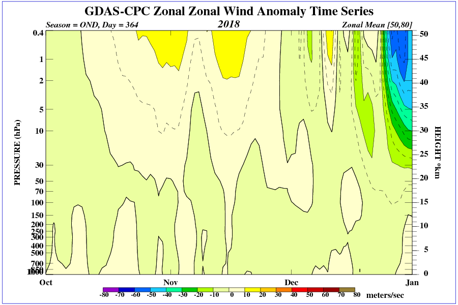
I remember that you were the first. However, it is interesting to associate with the dropping speed of the polar vortex.
Thanks ren
Leif, The curve is from the data given in the cited paper (Vieira, et. al., 2011, see the link in the post). It is different from your reconstruction, but you can’t know if it is wrong or right. Both your reconstruction and Vieira’s are approximations from proxies and anchored with suspect TSI measurements from numerous satellites that do not agree with one another. Basically all TSI reconstructions are suspect. You might remember my post on the subject, pay articular attentions to figure 11:
https://andymaypetrophysicist.com/2018/05/03/climate-change-due-to-solar-variability-or-greenhouse-gases-part-b/
One day we will know what TSI is and how it varies, but we do not know today.
Leif, The curve is from the data given in the cited paper (Vieira, et. al., 2011, see the link in the post). It is different from your reconstruction, but you can’t know if it is wrong or right
Your comment just shows that you have not taken the trouble to read by link where the reasons for my reconstruction are given.
If you maintain that one cannot know what TSI is, then you cannot use it as an argument.
“our comment just shows that you have not taken the trouble to read by link where the reasons for my reconstruction are given.”
Leif, You should remember that I have read your ppt, we’ve discussed it in detail several times before. We have already discussed the fact that slides 59-63 make my point. This quote from slide 62 is appropriate: ” TSI measurements perhaps not as stable as thought.”
Or from 63:
“Possible problems with the calibration of TSI records”
When it comes to satellite measurements of TSI, both statements are obviously true. And, if we do not know what TSI is today, how do we know what it was in the past? How well does it correlate with sunspot counts? Basically, we don’t have a clue, but at some point in the future we probably will know, we just don’t know today. We shouldn’t pretend we do know.
Possible problems with the calibration of TSI records
That pertains specifically to the SORCE TIM record. The Belgian record does not have that problem.
The uncertainty here is very small [about 0.1 W/m2] and does impair the long-term record. That you hang your hat on that just shows that you have not understood anything.
The Vieira reconstruction [2011] was based on the old [outdated] Hoyt&Schatten group sunspot number combined with an invalid assumption [that the ‘base’ value of TSI varies as the running 11-yr mean of the group number]. That you show an out-of-date reconstruction just shows that you are activist and not a scientist.
Solar activity has not changed secularly the last 300 years [as your Figure 4, upper panel shows, and as the current Version 2 shows]. The magnetic flux depends strongly on the sunspot [or group] number and TSI depends directly on that flux as I show on Slide 52 [and as everybody else agrees with]. Conclusion: your lower panel Figure 4 is misleading and simply plain and shamefully wrong.
and does NOT impair the
Because variations of TSI is directly caused by the magnetic field which we can get from both cosmic ray proxies and sunspot records [ https://leif.org/research/Nine-Millennia-of-Multimessenger-Solar-Activity.pdf ] we can reconstruct TSI with confidence. Here is the record for the last 1000+ years:


Contradicts your Figure 4.
Leif,
Perhaps it eliminates or reduces known systematic errors.
Thanks for clarifying the curves on your plot, looks like I was correct in my assumptions.
My point is 95% over 7 years is not good enough to project a secular trend with confidence. From Kopp, 2016 (J Space Weather & Space Climate):
Thus, I’m not saying you are wrong, just that the data are not good enough to demonstrate you are correct. An undetected, climatically significant secular trend in solar irradiance could exist and we are not seeing it. Your “solar activity floor” at sunspot minima may exist and be flat, but the data are not good enough over a long enough period to demonstrate that. Instrument stability at that level has not been achieved yet for long enough periods as demonstrated by Kopp, 2016.
https://www.swsc-journal.org/articles/swsc/abs/2016/01/swsc160010/swsc160010.html
looks like I was correct in my assumptions.
No, you were not correct. The blue curve was not ‘raw’ data.
Instrument stability at the needed <0.001%/yr level has not been achieved
Out of context. Needed to detect the solar luminosity evolution, less than 0.014 W/m^2.
Thus, I’m not saying you are wrong, just that the data are not good enough to demonstrate you are correct.
They absolutely are. You should not hide behind your ignorance argument. It takes perhaps a bit of courage to admit that you do not understand the issue. Man up.
My point is 95% over 7 years is not good enough to project a secular trend with confidence
You totally misunderstands this. The point has nothing to do with the secular variation, but with how much of the variation is predicted by the model as being due to the variation of the magnetic field.
This makes the argument of the near constancy at solar minimum compelling: if there is almost no magnetic field left TSI must converge to almost the same value regardless of time. This holds over the thousands of years covered by the cosmic ray proxies.
As https://arxiv.org/pdf/1711.04156.pdf notes:
“The remarkable agreement between the model and the measurements cogently demonstrate that our understanding of these mechanisms, and the TSI variability in general, is fundamentally correct“.
Leif, No need to rehash an old argument, we have both made our case, the readers can decide. But, I do not think TSI is known to 0.1 W/m^2 as this plot of the raw satellite measurements shows:

I do not think TSI is known to 0.1 W/m^2 as this plot of the raw satellite measurements shows:
There are two issues: the absolute value which is known to 0.5 W/m2 and the relative variation which is known to 0.1 W/m2. The latter is the one of interest. The various systematic errors have been identified and corrected.
And I don’t think you have made your case at all. Basically just shown your ignorance about the subject.
Especially since you have chosen a model based on outdated data.
Leif,
“the absolute value which is known to 0.5 W/m2 and the relative variation which is known to 0.1 W/m2.”
I agree with this part. relative variation is important for determining the amplitude of one solar cycle. Accuracy is important for determining long term (that is climatic) variation. For climate, the long term variation is what is needed and we do not know that accurately enough. Satellites last ~15 yrs and 0.5 x 30 years ~ 1 to 15 W/m^2!
Satellites last ~15 yrs and 0.5 x 30 years ~ 1 to 15 W/m^2!
Completely wrong. The absolute accuracy is over the entire interval, not compounded each year. And why year? Why not day or minute?
As per the experimenter:
“The TIM instrument is proving very stable with usage and solar exposure, its long-term repeatability having uncertainties estimated to be less than 0.014 W/m^2/yr (10 ppm/yr). ”
30 years x 0.014 W/m^2 = 0.42 W/m^2 [worst case is all errors went the same way].
Here is a comparison between the SORCE and TSIS [newest instrument on ISS] TSIs:

Their absolute difference in 0.47 W/m^2, within their stated uncertainty of 0.5 W/m^2.
Their relative difference [after correcting for the systematic offset] is less than 0.1 W/m^2 as you can see.
Come on, you are not too old to actually learn something [if willing].

The absolute accuracy of 0.5 W/m2 means that the value today is within that of the true value. And that the value a year ago was also within 0.5 W/m2 of the true value, and that the value 15 year ago was also within 0.5 W/m2 of the true value, etc.
“The absolute accuracy is over the entire interval, not compounded each year.”
This is possible, which why I gave the range of 1-15 W/m^2. The other problem with the satellite measurements is that the accuracy can drift with time, this is well documented. Thus the accuracy will be better when the satellite is new and worse after 15 years due to the solar radiation affecting the instrument. Over 30 years (a climatic time frame) I think the best we can expect is 1 W/m^2, the worse is 15 W/m^2. I think you misread what I wrote, or I didn’t explain it well enough. We agree here I think, except I still think the satellites to-date are not accurate enough to say we know TSI, I think we clearly do not know it well enough over climatic periods of time.
“The absolute accuracy is over the entire interval, not compounded each year.”
This is possible, which why I gave the range of 1-15 W/m^2.
If the absolute accuracy is 0.5 W/m2 it means that the range is is 0.5 W/m2. Not compounded every year.
Thus the accuracy will be better when the satellite is new and worse after 15 years due to the solar radiation affecting the instrument.
The degradation with time is monitored and corrected for by having several sensors, including one that is only exposed to the sun once every week or so.
I think we clearly do not know it well enough over climatic periods of time
We know it quite well over the past three centuries.
In any case, if you believe that you don’t know it, then you are not justified [as in Figure 4] to use it in your arguments.
Leif,
“If the absolute accuracy is 0.5 W/m2 it means that the range is is 0.5 W/m2. Not compounded every year.”
Only if one satellite can last with that sort of accuracy for 30 years. This has not happened yet. So far, the accurate satellites max out at around 15 years, this is why I’ve doubled the number, 2 satellites is 1 W/m^2, not 0.5. Look at the plot you posted below. I’m surprised you are missing this stuff, you must already know it.

Only if one satellite can last with that sort of accuracy for 30 years. This has not happened yet. So far, the accurate satellites max out at around 15 years, this is why I’ve doubled the number, 2 satellites is 1 W/m^2, not 0.5. Look at the plot you posted below
Now you are down to 1 W/m2 from your previous 15 W/m2, so some progress. But even so, that double number should not apply since 2003 where the accuracy stays at 0.5 W/m2. Furthermore the average of several overlapping measurements has a smaller error than just a single measurement.
The plot shows less than 0.5 W/m2, so look again.
Because TSI depends directly on the solar magnetic field that goes to almost zero at every solar minimum, TSI must also go to an almost constant value at every minimum. This puts a severe constraint on any long-term trend. As Schrijver et al. (2011) point out, TSI during the Maunder Minimum must have been close to what we observed at the last minimum in 2009.
Leif,
“Now you are down to 1 W/m2 from your previous 15 W/m2”
The range has always been 1 to 15, that has never changed, how you missed the one, but saw the 15 I have no idea. Nothing has changed. You even quoted me “1-15.”
This is still the correct range, given the instrument characteristics. Now, it will narrow with time if the instruments demonstrate the stability claimed by the designers, but believe the actual performance, not the advertising. I’m talking about knowledge we now have, not what we hope to have in the future.
“The plot shows less than 0.5 W/m2, so look again.”
The curves are not clearly labeled, but I assume the raw data are plotted with the blue and purple curves and the green curve is shifted, if so the difference is ~0.5 between the curves at mid-year. Each curve is +-0.5, for a total of one or more.
“Because TSI depends directly on the solar magnetic field that goes to almost zero at every solar minimum, TSI must also go to an almost constant value at every minimum. This puts a severe constraint on any long-term trend. As Schrijver et al. (2011) point out, TSI during the Maunder Minimum must have been close to what we observed at the last minimum in 2009.”
This idea is still a hypothesis IMHO. Perhaps so, but if true, why is there apparent variation in some solar activity indicators when there are no sunspots? In particular there is a lot of activity in the aa index at solar minima. I do not think this idea is universally accepted.
This is still the correct range, given the instrument characteristics
Not at all. The instruments had systematic errors [extra light entering the aperture] which were found and corrected for. Because they overlap we can normalize each instrument to a common scale [e.g. SORCE TIM]. This eliminates the systematic errors.
The curves are not clearly labeled
Again you are making unwarranted assumptions. Each curve is clearly labeled. TSIS is the pink, SORCE is the ]lower] blue. They have a difference of 0.47 W/m2 which is within their claimed accuracy. Reducing SORCE to the same scale as TSIS gives the green curve that matches the pink [TSIS] within 0.1 W/m2.
This idea is still a hypothesis IMHO. Perhaps so, but if true, why is there apparent variation in some solar activity indicators when there are no sunspots? In particular there is a lot of activity in the aa index at solar minima. I do not think this idea is universally accepted.
First, there is not a ‘lot’ of activity in the aa index at solar minima. The aa-index minimizes when the sun does. Second, There is a ‘floor’ in the interplanetary magnetic field so there is always some field to interact with the earth. Third, it is generally accepted that the variation of TSI is simply due to variation of the solar magnetic field, e.g. https://journals.aps.org/prl/abstract/10.1103/PhysRevLett.119.091102
“The variation in the radiative output of the Sun, described in terms of solar irradiance, is important to climatology. A common assumption is that solar irradiance variability is driven by its surface magnetism. Verifying this assumption has, however, been hampered by the fact that models of solar irradiance variability based on solar surface magnetism have to be calibrated to observed variability. Making use of realistic three-dimensional magnetohydrodynamic simulations of the solar atmosphere and state-of-the-art solar magnetograms from the Solar Dynamics Observatory, we present a model of total solar irradiance (TSI) that does not require any such calibration. In doing so, the modeled irradiance variability is entirely independent of the observational record. (The absolute level is calibrated to the TSI record from the Total Irradiance Monitor.) The model replicates 95% of the observed variability between April 2010 and July 2016, leaving little scope for alternative drivers of solar irradiance variability at least over the time scales examined (days to years).”
https://arxiv.org/pdf/1711.04156.pdf
“The solar brightness varies on timescales from minutes to decades1, 2. Determining the sources of such variations, often referred to as solar noise, is of importance for multiple reasons: a) it is the background that limits the detection of solar oscillations3, b) variability in solar brightness is one of the drivers of the Earth’s climate system4, 5, c) it is a prototype of stellar variability6, 7 which is an important limiting factor for the detection of extra-solar planets. Here we show that recent progress in simulations and observations of the Sun makes it finally possible to pinpoint the source of the solar noise. We utilise high-cadence observations8, 9 from the Solar Dynamic Observatory and the SATIRE10, 11 model to calculate the magnetically-driven variations of solar brightness. The brightness variations caused by the constantly evolving cellular granulation pattern on the solar surface are computed with the MURAM12 code. We find that surface magnetic field and granulation can together precisely explain solar noise on timescales from minutes to decades, i.e. ranging over more than six orders of magnitude in the period. This accounts for all timescales that have so far been resolved or covered by irradiance measurements. We demonstrate that no other sources of variability are required to explain the data.”
That you ‘don’t think so, is not a valid argument, just illustrates your ignorance.
Again, you should study https://leif.org/research/EUV-F107-and-TSI-CDR-HAO.pdf
There is even a Youtube presentation for your convenience:
Here is the assessment of the experimenters of the TSI uncertainty:
“The TIM instrument has long-term repeatability with estimated uncertainties less than 0.014 W/m^2/yr (10 ppm/yr). Accuracy is currently reported as 0.48 W/m^2 (350 ppm), but expected to decrease as calibrations are refined and incorporated. The TSIS/TIM agrees well with the lower TSI values first reported by the SORCE/TIM and the follow-on TCTE/TIM. The TIM design allows less internal instrument scatter than predecessor TSI instruments, which caused erroneously high TSI values (Kopp & Lean 2011), as validated on the TSI Radiometer Facility (described by Kopp et al. 2007).
The following paragraphs discuss the four different uncertainties reported with the TSI measurements.
INSTRUMENT UNCERTAINTY reflects the instrument’s relative standard uncertainty (absolute accuracy) and includes all known uncertainties from ground- and space-based calibrations plus a time-dependent estimate of uncertainty due to degradation. This value is currently reported as 350 ppm, but is expected to be refined lower with new calibrations and on-orbit validations. This uncertainty varies slightly with measured instrument temperature and the time to the nearest on-orbit calibrations. This value is useful when comparing different TSI instruments reporting data from the same time range on an absolute scale.
INSTRUMENT PRECISION reflects the TIM’s sensitivity to a change in signal, and is useful for determining relative changes in the TIM TSI due purely to the Sun over timescales of two months or less (so that degradation uncertainty does not have a significant effect). This value of 5 ppm [=0.07 W/m^2] is constant, and indicates the instrument’s noise level.
High-cadence Level 2 data are averaged (un-weighted mean) to produce daily and 6-hourly averaged Level 3 data. The standard deviation of the Level 2 values averaged to produce each Level 3 value is indicative of the solar variability during the reported Level 3 measurement interval, and is called the SOLAR STANDARD DEVIATION. This uncertainty redundantly includes — but is generally much larger than — the Instrument Precision. The Solar Standard Deviation is useful for estimating potential variations in TSI within the time range of a Level 3 data value, such as when comparing TIM TSI values with solar images or other TSI instruments reporting data at slightly different times.”
From http://lasp.colorado.edu/data/tsis/tsi_data/tsis_tsi_L3_c24h_latest.txt
Leif, I agree with Kopp and Lean’s assessment. Our only disagreement is whether current accuracy is good enough to judge the solar variability component in climate change, which the IPCC states is zero. I think the lack of long-term accuracy in our estimates of TSI (>30 years) is such that the effect could be significantly greater than zero and would not see it with current data. This really should not be controversial. The long-term data problems are clear.
I think the lack of long-term accuracy in our estimates of TSI (>30 years) is such that the effect could be significantly greater than zero and would not see it with current data.
The long-term accuracy has been 0.5 W/m^2 [not 15 W/m^2]. From that we can judge the dependency of TSI on the solar magnetic field which we in turn can estimate reliably at least the last 250 years, so we have a good handle on the long-term variation.
And the effect on climate is not zero as you think [or quote] but rather of the order of 0.1 degree due to solar variability.
The discussion on this should be interesting. Right now, all I can conclude is that no one has a robust model for climate.
Re. the Dalton Minimum and volcanic eruptions, it has long been observed that volcanism and earthquakes correlate statistically significantly with solar activity.
https://pubs.giss.nasa.gov/abs/st07500u.html
Thank you John:
What creates ‘climate’ is under our feet, not up in the sky.
Peta,
You’re welcome.
IMO celestial and terrestrial effects, and the interactions between them, combine to create climate and its changes. Climatology however is still in its infancy and far from settled. Its development has been stunted by thirty years of sheer lunacy, speaking of ET effects.
We don’t even have enough good data to begin to understand climatic changes on many time scales.
We don’t even have enough good data to begin to understand climatic changes on many time scales.
That does not seem to deter all kinds of fanciful claims to the opposite. To wit: this very post.
Leif,
Among the data we do have are length of day, cosmic ray and sunspot observations for at least some of the period covered, and defensible reconstructions for the rest.
Among the data we do have are length of day, cosmic ray and sunspot observations for at least some of the period covered
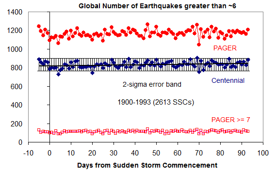

For that time where we have ‘good’ data there is no effect of solar activity on earthquakes. See the USGS analysis I refer to: https://phys.org/news/2013-04-link-solar-earthquakes.html
A superposed epoch analysis with geomagnetic [solar] storms also does not indicate any effect:
Leif,
The USGS, like GISS and NOAA, are not to be trusted.
The failure of that paper’s statistical analysis is glaring. Its sample is not significant and apparently cherry-picked, the same way that “data” on advancing v. retreating glaciers is massaged.
CACA orthodoxy has corrupted government “science” thoroughly and the academe to an almost equal extent.
The USGS, like GISS and NOAA, are not to be trusted.
Am I to be trusted? I find the same thing as USGS
Please see the study I linked from two years before your USGS source.
Thanks.
John
If you were around here some 7+ years ago you may have seen
this if not you might find one or two quotes interesting
Thanks!
Wow! Maybe piezo effects pushing stuff around? Any relation to earthquake lightning?
it has long been observed that volcanism and earthquakes correlate statistically significantly with solar activity.
Not so:
https://phys.org/news/2013-04-link-solar-earthquakes.html
“[1] We examine the claim that solar‐terrestrial interaction, as measured by sunspots, solar wind velocity, and geomagnetic activity, might play a role in triggering earthquakes. We count the number of earthquakes having magnitudes that exceed chosen thresholds in calendar years, months, and days, and we order these counts by the corresponding rank of annual, monthly, and daily averages of the solar‐terrestrial variables. We measure the statistical significance of the difference between the earthquake‐number distributions below and above the median of the solar‐terrestrial averages by χ2 and Student’s t tests. Across a range of earthquake magnitude thresholds, we find no consistent and statistically significant distributional differences. We also introduce time lags between the solar‐terrestrial variables and the number of earthquakes, but again no statistically significant distributional difference is found. We cannot reject the null hypothesis of no solar‐terrestrial triggering of earthquakes.”
We count the number of earthquakes having magnitudes that exceed chosen thresholds in calendar years…
Didn’t count the little ones?…..if they are looking to see if it triggers earthquakes…count them all
if they are looking to see if it triggers earthquakes
If the little ones cause the big ones, it suffices to count the big ones.
The little ones often relieve pressure, delaying the Big Ones.
The little ones often relieve pressure, delaying the Big Ones.
The links you have referred to did not show the little ones…
Leif,
You said “If the little ones cause the big ones, it suffices to count the big ones.” Is that an assumption that you are making? If so, is it just the number of ‘little ones” or might the total energy released be a more accurate metric?
What was the rationale for the thresholds that were chosen? Were they round logarithms, or were the magnitudes converted to energy? Each unit of Richter magnitude is approximately 32 times the energy of the previous unit, so the magnitude threshold can be critical. Was the depth to the focus considered in any way?
You could benefit from reading the USGS analysis I referred to:
https://agupubs.onlinelibrary.wiley.com/doi/full/10.1002/grl.50211
I quote from their introduction:
[2] In the search for reliable methods for predicting earthquakes, geophysicists have sometimes investigated natural phenomena that might affect their occurrence likelihood. In the context of critical‐point accumulation of stress on a fault, a small “nudge” might be all that is needed to trigger an earthquake. The list of unconventional phenomena that might provide such a triggering nudge is long, and their relative importance has historically been controversial [e.g., Omori, 1908]. The great solar astronomer Wolf [1853] suggested that sunspots could influence the occurrence of earthquakes. Qualitatively, a solar‐terrestrial effect on seismicity, if one exists, would almost certainly require some sort of coupling between the Sun, solar wind, magnetosphere, and lithosphere. This coupling might, for example, cause small changes in the Earth’s rotation rate, and these could result in more earthquakes [Sytinskiy, 1963; Gribbin, 1971]. Alternatively, magnetic storms might induce eddy electric currents in rocks along faults, heating them and reducing their shear resistance [Han et al., 2004], or induced currents might cause a piezoelectric increase in fault stress [Sobolev and Demin, 1980]. In either case, earthquakes might be triggered. These theories are speculative; they have not yet been sufficiently developed to permit reliable predictions of future earthquake occurrence probability.
[3] A number of published papers have reported, from empirical analysis of historical data, that there is a detectable nonrandom relationship between solar‐terrestrial interaction and earthquake occurrence. Some of these reports are inconsistent with each other, and some are based on only selected subsets of the available data. For example, over long time scales, global seismicity has been reported to be highest during solar‐cycle sunspot maximum [e.g., Odintsov et al., 2006] and, very differently, highest during the declining phase and minimum of the solar cycle [e.g., Simpson, 1967; Huzaimy and Yumoto, 2011]. Over shorter time scales, global seismicity has been reported to be correlated with solar‐quiet geomagnetic variation [e.g., Duma and Ruzhin, 2003; Rabeh et al., 2010], with geomagnetic disturbance [e.g., Simpson, 1967], and with enhanced solar wind velocity [e.g., Odintsov et al., 2006]. There have also been reports that regional seismicity is correlated with magnetic‐storm occurrence [e.g., Sobolev et al., 2001; Bakhmutov et al., 2007]. Some reports have focused on a few large earthquakes [e.g., Mukherjee, 2006; Anagnostopoulos and Papandreou, 2012].
[4] The statistical significance of a possible correlation between sunspots and seismicity has occasionally been questioned [e.g., Jeffreys, 1938; Meeus, 1976], and for certain geographic regions, correlation between solar‐terrestrial variables and seismicity has actually been shown to be insignificant [e.g., Stothers, 1990; Yesugey, 2009]. Still, reports that identify such correlations continue to be published, especially lately. The public finds the possibility of a causal connection between the Sun and earthquakes to be interesting, as evidenced by the speculative accounts that are sometimes published in the popular press [e.g., Hudson, 2011] and the need for the U.S. Geological Survey to post responses on its website to related “frequently asked questions.” In light of all this, and in recognition of the importance of earthquake prediction, we are motivated to conduct our own retrospective analysis of historical data recording sunspots, solar wind, geomagnetic activity, and global earthquake occurrence. In the spirit of classical hypothesis testing [e.g., Stuart et al., 1999, chapter 20], we seek to reject the null hypothesis that solar‐terrestrial interaction plays no role in triggering earthquakes.
2 Inspection and Selection Biases
[5] Given two statistically independent time series of finite duration, it is always possible, with retrospective inspection, to find an illusionary relationship of some type. For example, it has been claimed that stock market performance has, in the past, been correlated with the phases of the moon [e.g., Yuan et al., 2009], a conclusion that some researchers assert was obtained after subjectively searching data sets until something seemingly “interesting” was found [e.g., Crack, 1999]. This correlation lacks a known causal basis, and by retrospectively focusing attention on its presence, one might be seduced by “inspection bias.” To avoid this, the correlation should be shown to be both persistent and detectable in a second “objective” data set that was not used in the original identification of the correlation. Ideally, an entirely new objective data set should be prospectively collected—after—predicting a correlation of the same type as seen in the first data set [e.g., Feynman, 1998, pp. 80–81]. “Significance” is assigned if a correlation of the size measured in the objective data set would be an unlikely realization from a null‐hypothesis random process. While many published geophysical reports quote retrospective probabilities of correlational “significance” using the very same data used in the identifications of the correlations, technically, these can only support either pessimistic or neutral conclusions. If a retrospective significance probability is large, then the null hypothesis of randomness cannot be rejected, and the persistence of the correlation must be regarded with skepticism, even without consideration of a second objective data set. If a retrospective probability is small, the correlation cannot be regarded as persistent until a significant correlation is shown to exist in a second objective data set.
[6] Related to all of these issues are the the difficulties posed by “selection bias” [e.g., Mulargia, 2001]. It is natural for the attention of a scientist to be drawn to rare and unusual occurrences, such as the “clustering” of several geophysical events in time. It is even sometimes tempting to consider more isolated occurrences, such as a single great earthquake that happened to be preceded by a magnetic storm or a longish duration of magnetic disturbance. A pair of unusual events can represent an opportunity for new insight, provided that the temporal relationship of the events has a valid causal explanation. Otherwise, there is the danger of falling for a logical fallacy—just because one event occurs immediately before another does not mean that they are related [e.g., Woods and Walton, 1977]. More generally, a correlation that might have seemed interesting in a small and subjectively selected data set will not necessarily be measurably significant in a second objective data set. In which case, the null hypothesis of randomness cannot be rejected, and the persistence of the correlation must be regarded with skepticism. If, for whatever practical reason, a subset of the available data must be selected, then, for objectivity, the selection should be made on the basis of properties that are independent of the statistical properties being analyzed.
Leif,
Thank you for the link. While you did not address my questions, the article did. Specifically, the authors only considered earthquakes of magnitude 7.5 (nominally like the Loma Prieta event) and greater, with thresholds at 0.5 magnitude increments, as I speculated. That is, they were dealing with logarithms of the energy, rather than the energy, with increasing widths of the energy bins. The very largest earthquakes were sufficiently rare to call into question the ability to say anything definitive about their statistical significance. And, as I suspected, they did not consider the depth of focus, which is important because the mechanisms for release are probably different. That is, the small, shallow earthquakes occurring in the brittle upper crust would probably be more prone to experiencing the deceleration effects speculated by Javier. So, I agree with Latitude, that a thorough examination should include ALL instrumentally detectable earthquakes, not just the very large ones.
In summary, probably the very largest earthquakes are not triggered by changes in deltaLOD, but that doesn’t rule out smaller ones. And, John Tillman is right, that the prevailing view is that small earthquakes relieve accumulating strain and forestall very large earthquakes, i.e. increase the lag time.
While you did not address my questions, the article did.
No need for me to repeat what the article said.
So, I agree with Latitude, that a thorough examination should include ALL instrumentally detectable earthquakes, not just the very large ones.
The [BIG] problem with that is that our instruments have become much better with time, so the dataset would not be homogeneous but would show an [artificial] increasing secular trend.
It is the mark of bad science to postulate an effect that cannot be reliably measured.
Big earthquakes almost always cause a huge swarm of little ones as the locked plate boundaries establish a new equilibrium, no?
And big ones often have no small ones preceding them…they are abrupt and impossible to anticipate, except to the extent that large scale patterns of strain and relief can be mapped and probabilities assigned to various zones along a well studied fault, giving some idea of the potential magnitude and long term likelihood of future quakes within a certain region…but these are vague and data is sparse.
How many years of data might be needed to make predictions more likely to have significant value in places where large earthquakes recur with some periodicity?
I suspect that no amount of studying trends will ever allow specific predictions for specific sections of a given fault, since what really matters are the physical irregularities in the locked fault segments combined with the strength of the locked rocks themselves.
For examples, some segments of the San Andreas have few such irregularities, and the strain resulting from the plate movements is dissipated by numerous and frequent small quakes.
Other segments are locked by large irregularities in adjacent plate boundaries, and huge amounts of strain must build up before the mechanical strength of the rocks is overcome and the fault slips massively and suddenly.
Consider that the only way we really know if a quake is a foreshock, or a main shock, is after a considerable length of time has passed.
Just sayin’.
Just sayin’.
In effect that solar activity is not a good predictor of earthquakes.
I think we can agree on that.
Leif,
You said, “No need for me to repeat what the article said.” Then why did you “repeat” five LONG paragraphs?
You also said, “The [BIG] problem with that is that our instruments have become much better with time, so the dataset would not be homogeneous but would show an [artificial] increasing secular trend.” That is not a unique problem in science when historical data are being used to establish trends. As is usually the case, one has to find ways to work around the limitations, such as setting a threshold (<<M7.5) that was attainable prior to digital electronics.
You also pontificated with "It is the mark of bad science to postulate an effect that cannot be reliably measured." Einstein theorized about the effects of relativity before they were measured, and they continue to be measured with increasingly precise instrumentation to this day. Indeed, it is the inductive postulates that lead to experiments that can be used to test the null hypothesis, and advance science.
“In effect that solar activity is not a good predictor of earthquakes.
I think we can agree on that.”
Regarding specific locations and specific timing, for sure we agree.
Whether there might be some statistical correlation over the entire earth seems to be a different question, because it is likely the case that at any given time there are some places that are very close to the mechanical breaking point of the rocks locking the fault, and only small additional forces (or some small weakening of the rocks) is required to cause them to break and an earthquake to occur.
It seems to me the period of time that scientists have been able to measure every earthquake, no matter where or when it occurs, is short…too short. I am uncertain of how long and how carefully such things as Telluric currents have been measured, or whether it has been demonstrated that piezo-electric effects and such are large enough to make much difference in the strength of rocks or resistance to breaking under strain.
In short, I personally am agnostic regarding whether such effects as solar cycles may cause could possibly influence earthquakes (or other geologic phenomenon such as volcanic eruptions), both because I do not know a whole lot about it, other than some think there is a correlation, and because I am unsure if enough information exists to decide one way or another.
I am skeptical, but open minded on the issue.
IOW…maybe so, maybe no, but it is interesting enough to merit study, IMO.
There is much we do not know, or that I am certain, even in regards to things which are hiding in plain sight.
After all, how long ago were such phenomenon as sprites and other forms of upward directed electrical discharges from thunderstorms either unknown or dismissed out of hand by those who reported seeing them?
Even now I do not think there is much consensus one way or the other regarding phenomenon associated with earthquakes such as sounds and lights, but there does seem to be accumulating evidence that some peculiar things sometimes occur just before or during earthquakes.
Now that huge numbers of cameras are both always turned on and carried around by people, we may know more in the near future.
Solar-seismic connection:
http://www.academia.edu/1827859/Influences_of_Solar_Cycles_on_Earthquakes
I was thinking that since low solar allows cosmic rays to penetrate farther into the atmosphere, is it possible that during low solar high energy pions/protons penetrate into the Earth’s crust causing increased heating in magma chambers and subduction zones?
JerryG
Bravo! Bravo! Bravo! This is reality.
Well, focusing on gradients is correct but I don’t think the above post has it right. It does, however, refer to the importance of zonal / meridional air flows that I have been drawing attention to for more than ten years here and elsewhere.
You don’t need to vary the Earth’s rotation speed in order to have solar variability change the gradient of tropopause height between equator and poles and I believe it is that gradient which causes climate variability within the troposphere via changes in zonality / meridionality and consequently total global cloudiness rather than the gradient of temperature per se.
http://joannenova.com.au/2015/01/is-the-sun-driving-ozone-and-changing-the-climate/
This is gold….The poles are energy sinks to space (particularly in winter) and the efficiency of the poleward heat transport determines how much energy the planet retains, not the amount of CO2 in the atmosphere, which has a much smaller effect. We are studying the thickness of the glass in the windows, when it is the open door to the poles that matters regarding warming.
And opens the door to the role ozone plays in creating pressure gradients. Go to https://reality348.wordpress.com. Erl Happ has collected a lot of trends.
Perhaps not simply the thickness of the glass, but whether adding another coat of black paint to the window will make the house darker inside or not.
Unfortunately the Image is a bit clipped -a paper linking major earthquakes to Solar Cycle Phases (ieee extract) :
https://www.semanticscholar.org/paper/Possible-correlation-between-solar-activity-and-Huzaimy-Yumoto/63846d3af8d5db1db300f2f7e2bf12e43b026ef3/figure/2
Note the Magnitudes, so simple statistical averaging will mask this :
Exogenous parameter is basically referred to the external activities that may have been the important factors in modulating the atmosphere, ionosphere and the earth’s surface. Due to its significant impacts, there is possibility to link solar activities and seismicity. Associated investigations have been done by previous researchers in order to explore the solar – terrestrial connection; nevertheless, the physical mechanism is still controversial. To comprehend the investigation of this coupling mechanism, we propose another exogenous source to be analyzed which is cosmic ray.
Secondary galactic radiation is concentrated in specific areas of the lower stratosphere during low solar activity.
Interesting.
“…and how the theory of ice ages (now termed glaciations) fitted in.”
Oh, well, I could not go further than this point in this article.
The terminology as per this, or up to this point very intricate and misleading!
Javier, if you care to reply to this comment, please tell about this ice age theory of yours, what actually do you mean by that.
In terms of climate such does not even happens to be there, as far as I know!
The most about ice ages consist in the term of explanatory guesses, at most, not even in the real of hypothesis to be consider it.
Also the data there quite clearly debunks the ice age concept, as per climate, as it clearly debunks it as per mean of it definition…
I am waiting for your theory of ice ages, and I guess I will be waiting for a very long time….as there no such thing at all…unless the definition of a theory or hypothesis these days simply mean “any clever or intelectual bollocks”.
I still stand and wait to be corrected in this one, by you Javier…hopefully me wrong and you right in this one.
Still must tell you to really consider the definition and the proper meaning of the “ice age”, before you may consider to reply…very much different than that of “glacial period”…
According to the orthodox basic climatology, there could no be a glacial period outside the ice age, but there still could be a ice age without a glacial period…only one of this depends in the other as per the definitions of this two concepts.
Hope you take the trouble and clarify the position about the above, provided that you can.
cheers
Whiten,
If I may reply while awaiting Javier’s response, you might be confused by the loose terminology used in popularized geology. “Ice age” can mean different things in common usage. Colloquially, it may refer to a glacial advance within a technical ice age.
“Glaciation” now signifies an ice sheet advance within an ice age, ie an interval with continental ice sheets. The present, Cenozoic Ice Age began about 34 Ma with the Oligocene formation of ice sheets on Antarctica, which waxed and waned during the Miocene Epoch. About 2.6 Ma, Pleistocene ice sheets also grew in the Northern Hemisphere. Greenland might have sported one even in the Pliocene Epoch, or at least an ice cap.
Between glaciations are interglacials, such as now, in which ice sheets disappear from some continents, or recede dramatically. Within glaciations are stadials (advances) and retreats (interstadials).
In geological terminology, there are also “Ice Houses”, long phases of Earth history in which climate is generally colder and ice ages may occur. There were at least two in the Paleozoic Eon, at the Ordovician-Silurian boundary and a longer-lasting one in the Carboniferous and Permian Periods.
During the Mesozoic Ice House, ice sheets didn’t develop, although there were seasonal ice and possibly montane glaciers on high peaks at times. That era however is better known for its Hot House climates, as during the mid-Cretaceous Period.
John.
Thank you for the reply, really appreciated.
You done your best there, I assure you, I do understand what you say…
but you see, you not answering the point…no ice age theory there.
I assure you, that am very well tuned to the colloquial meaning in this matter.
You see, there can be only one “Ice Age”, as that happens to be the naming of the last glacial period.
It is not an addressing of any ice ages, and the colloquial consequence is that ” Ice ages” mean glacial periods, not at all meaning ice ages.
According to the definition, even at the top of Iterglacial optimum, we were in an ice age, and still there, but no way to consider that we were then or now in a glacial period, or as colloquially considered an “Ice age”
Besides, unless Javier explains it, still Javier stands to be considered wrong and very messy,
as far as I can tell, and also very misleading, either by intention or not!
Still waiting for the theory or the hypothesis of ice ages.
Sorry got to say, beside of your explanations still no such theory or hypothesis there to consider yet.
Sorry for seeming somehow pedantic, but conclusions, guesses or even explanations do not actually consist as theory, no matter how clever or intellectually served.
And in this context I am quite sure I be there for ever in waiting for the “theory of ice ages”, or hopefully get to be educated and shown me wrong understanding in all this.
Thank you, really appreciated John
cheers
By “theory”, then I suppose you mean what causes ice ages. We know that Milankovitch cycles largely explain ice sheet advance and retreat, especially the axial tilt cycle, it appears.
On the larger scale, ice houses seem to occur at about 150 million year intervals, such that cosmoclimatologists point to Earth’s bobbing up and down during its orbit with the solar system around the galactic barycenter.
Tectonics appear to control at least in part whether an ice age will develop within an ice house interval. Conditions weren’t favorable during the Mesozoic, but where twice during the Paleozoic and now in the Cenozoic.
But naturally there is still much to learn.
Sorry John, but that is the very problem of the mess there.
Considering the M cycles, all that thing is not even a proper theory for glacial periods.
Nothing to do with ice ages, John…please try to get it right.
Milankovitch, a very good scientist, his M cycles hypothesis not so good to explain glacial periods, especially the Ice Age…
This guys hypothesis only concerning glacial periods…and ice ages are no glacial periods as per orthodox climatology, far longer far longer than glacial periods, different definitions.
Milankovitch hypothesis not the theory of ice ages…..there is no theory f ice ages…wake up John…sorry for being again somehow pedantic…probably should not comment in one to many drinks… 🙂
thanks.
cheers
cheers
Whiten,
M cycles don’t explain the onset of an ice age, ie the beginning of glaciation cycles. M cycles exist whether there are ice sheets or not. But they do explain glacial and interglacial cycles within ice ages.
This is why thinking clearly about ice ages requires adequate terminology.
For an ice age, first you need an ice house climate. Then you need a particular alignment of tectonic plates. But once you have an ice age, then the ice sheets will wax and wane with the celestial and orbital cycles described by Milankovitch and his predecessors.
Still waiting for the theory, john, the ice age theory, and that in not, sorry, regardless of any explanations there, for what required, no theory I can consider…
No ice age theory no consideration of even hot or cold houses there…even worse, ice age debunked forget of any thing about houses …
As far as I know, the data there, does really debunk the concept and the meaning of ice ages in its very definition.
Oh well, still waiting for the theory, or even a hypothesis of ice ages…..tic-toc-tic. ””””””””””” :-0
cheers
Whiten,
Please provide data debunking the fact of ice ages.
I’m still unclear as to of what you imagine the “theory” of ice ages to consist. That they exist is an observation, ie a scientific fact.
Thanks!
John Tillman
December 12, 2018 at 1:16 pm
“Whiten,
Please provide data debunking the fact of ice ages.”
————-
a simple answer to your simple request:
The age of ice in Antarctica, does debunk the ice age definition.
If you know what the age of that ice there is, than you got to consider what the age of Antarctica ice shelf, or ice cup is…
it could easy be considered as in billions of years old, if the age of ice there ~35 millions years old…simple as that, not easy to dismiss it, or arbitrary ignore it, especially when there no any theory or hypothesis of ice ages…
but very easy to be considered as at least in hundred of hundreds of years old…much more longer, far longer, than the ice age claim and definition of it can afford, in any case…something to do with fairly basic concepts and numbers…no much
“rocket science” required there.
Oh well,any thing like M cycles or AGW will do for a consideration of at the very least a hypothesis…while far more harder when considering theories…some thing like similar to the classical old one theory of Solar system…
cheers
Oh correction needed:
“but very easy to be considered as of at least in hundred of hundreds years old”
where “at least in hundred of hundreds years” meant to be:
“at least in hundred and hundreds of million years”
Thorry for the mess… 🙂
cheers
Are you trying to make sense or are you just trying to be tripe? in all sincerity i really hope you are not actually trying to make sense.
Bob
I sense that Whiten is being coy and trying to demonstrate his intellectual superiority. He may have a point, but he seems to have a problem in stating it clearly.
Clyde I may be wrong but, my point in the mains of subject is very clearly stated…
but hey it needs that one be well comprehensible with all the mess of terminology and smoke and mirrors there.
Main point…me still waiting to hear the theory or even the hypothesis of ice ages…
whatever the imagination of one about it may or could be…very clearly stated…
how much clear than that a point can be stated?!
Still waiting.
cheers
thanks.
Whiten
Your grammar is a little strange. This may be a language problem. Is English a second language for you? If that is the issue, then perhaps we can work through it.
Clyde, thank you for your reply.
Yes, English is not my first language.
Yes, I am still prone to error, as maybe any body else could be, even when considered not strictly in the context of;
whether English is or it is not my first language.
But still, I will consider it very helpful, if you can show me the “little strange grammar”
of mine in regard and connection to my reply comment to you.
Also, still open to some kind of help you may offer in regard to my other previous comments and the grammar problems there.
I am very aware and fully acknowledge that my English really messy or even very messy at times. 🙂
But still trying me best.
thanks… appreciated
cheers
Whiten,
Following are some suggestions. It isn’t always clear what you are trying to say, so my suggestions may not be correct.
“The terminology as per this, or up to this point, IS very intricate and misleading!”
“Javier, if you care to reply to this comment, please … EXPLAIN this ice age theory of yours”
You said, “Still waiting for the theory or the hypothesis of ice ages.” It isn’t clear to me whether you are implicitly complaining about what you think is an inappropriate use of the term “ice ages,” of if you are looking for a complete explanation for the processes that cause continental glaciation, and the processes and events responsible for inter-glacial initiation and termination.
In reviewing the exchanges above, I feel that Tillman did a reasonably good job of explaining the consensus view of the relationship between ‘M cycles’ and glaciation. But, it didn’t satisfy you. So, I am not clear on whether you are having difficulty understanding his explanations, or if you have some specific point to make that isn’t coming across. I suspect that it is an issue of definitions, but I can’t be sure. However, Tillman, Boder, Menicholas, and I are having a problem understanding just what it is that would satisfy you. Therefore, because I don’t really have a dog in this fight, it isn’t worth my time to try to edit all your comments and try to understand your point(s).
I tried, I really tried…but came away scratchin’ me achin’ ‘ead.
Whiten, Javier may not be able to join in this discussion due to other committments. His main post on glacial cycles, during the current ice age (we are still in it actually) is here:
https://judithcurry.com/2016/10/24/nature-unbound-i-the-glacial-cycle/
Whiten, here is a recent post by Javier on his prediction of the next glacial.
https://judithcurry.com/2018/08/14/nature-unbound-x-the-next-glaciation/
And the albedo.
Regarding the Dutton/Brune Penn State METEO 300 chapter 7.2: These two professors quite clearly assume/state that the current 0.3 albedo would remain even if the atmosphere were gone or if the atmosphere were 100 % nitrogen.
This is just flat ridiculous.
Without the atmosphere or with 100% nitrogen there would be no liquid water or water vapor, no vegetation, no clouds, no snow, no ice, no oceans and no longer a 0.3 albedo.
The sans atmosphere albedo would be much as the NASA moon data lists, a lunarific 0.12, 390 K on the lit side, 100 K on the dark.
And the w/o atmosphere earth would receive 25% to 40% more kJ/h of solar energy and as a result will be 20 to 30 C hotter not 33 C colder, a direct refutation of the greenhouse effect theory.
Nick S.
https://www.linkedin.com/feed/update/urn:li:activity:6466699347852611584
https://www.linkedin.com/feed/update/urn:li:activity:6457980707988922368
On a Snowball (or Iceball) Earth, the planet’s albedo might be higher than 1.0, like Saturnian moon Enceladus’.
John
How does one get an albedo greater than 1.0? Is that like “The Little Train That Could” putting out 120% effort?
https://en.wikipedia.org/wiki/Albedo
https://astronomy.stackexchange.com/questions/20795/why-is-enceladuss-albedo-greater-than-1
John,
From the wiki’ article I linked: “Enceladus, a moon of Saturn, has one of the highest known albedos of any body in the Solar System, with 99% of EM radiation reflected.”
Strictly speaking, albedo is the apparent brightness of diffusely reflecting celestial bodies, and for a body with diffuse reflectance and an albedo of 1.0, means a reflectance much less than a a perfect flat mirror because the mirror will return all the light to the source. Whereas, a diffuse body will scatter the same light flux over at least a hemisphere. So, comparing two diffuse reflectors, one may look brighter than the other, but neither will be returning to the observer anywhere near 100% of the light impinging on them.
For any body that might have an albedo apparently greater than unity, I would suspect that it fails the test of being a diffuse reflector and probably has a strong specular component with a preferred orientation that ‘focuses’ light towards the observer, at least for certain geometric alignments. Notice that when in an airplane, and flying among clouds, they all appear essentially the same brightness on the sunlit sides. One can’t have 98% of the light reflected off one side, move 90 degrees around it and still have 98% for the new side. That is why albedo is an apparent brightness, taking into account the maximum possible ‘reflectance’ in any particular direction.
That is the essence of the WUWT article I previously wrote on why albedo is the wrong metric for Earth when talking about how much light is absorbed on the surface. With the 70% of the Earth that is water, the light not absorbed is a mixture of both diffuse reflectance from suspended particles, and specular reflectance off the smooth surface. The diffuse reflectance is a back reflectance, while the specular reflectance is a forward reflectance.
Clyde,
Depends on how you measure albedo.
Citing Wiki, Eceladus’ albedo is either 1.34 or 0.81:
https://en.wikipedia.org/wiki/Enceladus
The higher figure is its geometric albedo at 550 nm:
http://science.sciencemag.org/content/315/5813/815
John,
W/o atmosphere there will be no water, snow, ice, clouds, vegetation or oceans to “freeze” at 394 K, 121 C, 250 F.
That’s the exact opposite of a greenhouse effect.
Enceladus has a water vapor atmosphere:
https://www.nature.com/news/2005/050314/full/050314-15.html
So?
Enceladus is WWAAAAYYY out there where it is COLD!!!!
1,434 E6 km vs 149.6 E6 km.
Solar constant for Saturn is 15 W/m^2, 127 K, -146 C.
Climate change and long-term fluctuations of commercial catches: the possibility of forecasting.
FAO Fisheries Technical Paper. No. 410. Rome, FAO. 2001. 86p.
http://www.fao.org/docrep/005/y2787e/y2787e00.pdf
In this FAO report the authors found a 6 year lag of Dt to LOD. See page 10:
2.1 SUMMARY
A phenomenon of close correlation between the main climatic index dT and geophysical index (-LOD) still remains an intricate puzzle of geophysics. Another challenging puzzle is the observable 6-year lag between the detrended run of dT and -LOD. Taking into account this lag, the LOD observations can be used as a predictor of the future climatic trends. Even without a mechanism for a causal relationship between the detrended climatic (dT) and geophysical (LOD) indices, the phenomenon of their close similarity for the last 140 years makes LOD a convenient tool to predict the global temperature anomaly (dT) for at least 6 years ahead.
[LOD = length of day? But that doesn’t match “geophysical features” since LOD doesn’t vary over centuries, only with latitude and day-of-year. . .mod]
Thanks to interactions between Earth and its atmosphere, LoD does vary on time frames of weeks to years, within its general trend of increasing length.
https://en.wikipedia.org/wiki/Day_length_fluctuations
Improvements in measruement precision and accuracy have enabled scientists to observe these variations.
mod,
“since LOD doesn’t vary over centuries, only with latitude and day-of-year.”
LOD Length-of-Day has nothing to do with daylight, this geophysical parameter refers to the rotation of the solid earth and as such is a planetary metric (nothing to do with latitude or the annual seasons).
For further information see the International Earth rotation and Reference systems Service (IERS)
http://hpiers.obspm.fr/eop-pc/index.php
I wonder if the “precipitable water” calculations behind Wisconsin’s graphic animation might be useful in computing a more complete accounting of the effect. There are instances when the flow of water vapor into Alaska is very pronounced, as is a southerly flow of relatively dry air down from Canada into the Midwest. The difference in mass flows, and where the mass is lost from the atmosphere, would seem to be the key. Presently, 1900 UTC this date, relatively little moisture is penetrating 50 N, so I would expect a rather small increase in the rate of rotation, assuming that the flows on the opposite side the NH are similar.
http://tropic.ssec.wisc.edu/real-time/mtpw2/product.php?color_type=tpw_nrl_colors&prod=namer×pan=24hrs&anim=html5
I really appreciate posts like this one. It offers a real alternative to the indoctrination that poses as an education in America today.
See the flow of water vapor above the Barents Sea.
http://tropic.ssec.wisc.edu/real-time/mtpw2/product.php?color_type=tpw_nrl_colors&prod=europe×pan=24hrs&anim=html5
Javier-
Found the article interesting. Thank you for posting it.
Regards,
Max
P.S. Good luck with the verbal food fight in the comments.
Why is the above post by Javier, editable on my mobile phone? I can add and remove text and images. Most posts are not editable in this way. WUWT?
(The edits are being done in YOUR Phone not in the WUWT blog itself) MOD
Tasfay,
Thanks for letting us know. We are looking into it.
Andy
Thanks Andy
I hope no-one else saw the edits that I made!
Tasfay, No your edits were only on your computer or phone, if you hit refresh it will go back to the way it was. There much be some imbedded code that allows the user to edit the post. We don’t know how it got in there, but it seems harmless enough. We tried a few fixes, but the problem is still there, just ignore it and press refresh if you change anything.
I added “(the Great and Powerful)” after Javier’s name, but obviously it didn’t stick.
I’m surprised no mention of Theodore Landscheidt’s work…Linked below…
http://bourabai.kz/landscheidt/publications.htm
He claimed even the sun rotates around a ‘barycenter’, the ‘physical’ center of our solar system. The planets pull the sun around in different ways over time.
Willie Soon has a lecture on this topic:
https://wattsupwiththat.com/2018/09/22/evidence-the-sun-may-have-turned-blue-during-1450s-1460s/
Javier.
You really need to give us predicted LOD for the next 20 years, so your thesis can become predictive.
.
And just thinking without researching, but surely a major contributor to Delta LOD with the seasons, would be the build up of snow and ice at the northern pole. If you concentrate mass on the axis a body will spin faster, like an ice-skater pulling their arms in. And since the major continents and ice sheets reside in the north, the northern winter-summer differential will have the greatest effect.
This would mean a corellation between LOD and northern winter snow extent. Just eyeballing the two side by side that may be true, but I have not plotted the two datasets together yet.
R
Javier: “The importance of the latitudinal temperature gradient cannot be overstated”
WR: Agree. Cold poles have all kinds of effects. The main thing for the average temperature of the Earth is the lack of water vapor during colder circumstances at the poles. This lack of water vapor enables a lot of polar radiation to reach space with the speed of light. Directly. And without any (!) delay by absorption and consequent thermalization of the energy. Gone is gone: cooling the surface.
But in case of warming of the poles more energy is retained near the surface of the poles by a higher content of water vapor, causing a higher temperature. Water vapor is our main absorbing (‘greenhouse’) gas. That rise in water vapor content especially happens in the Arctic area which is easier to influence because of the possibility to melt [more] ice. By consequence the water vapor content of the local atmosphere is enhanced easier and so the retardation of surface radiated energy.
No water vapor in the air causes cooling and cooling of a pole causes a strong pole – equator gradient with enhancement of other cooling processes.
That is why the Arctic is our main ‘swing area’ in climate. Any warming or any cooling has big effects on the Earth’s climates.
And why a big feature of hot house climates is “equability”, ie less difference between the poles and tropics.
Poor Mother Gaia has enjoyed no crocodilians in her polar cupboards for most of the Cenozoic.
John Tillman: “And why a big feature of hot house climates is “equability”, ie less difference between the poles and tropics.”
WR: Indeed. A reversal of the main vertical circulation in the oceans is able to create such an equality, as explained in https://wattsupwiththat.com/2018/06/15/how-the-earth-became-a-hothouse-by-h2o/
Warm poles with absorbing H2O everywhere in the air diminishes the total heat loss by the Earth, creating an overall warmer Earth, while the tropics even experience lower temperatures. The difference is made by the enormous rise in temperatures at the higher latitudes. Warm deep water transport and absorbing water vapor make the difference.
Wim,
As a renowned naval aviator was wont to say, “People are smart when they agree with you!”
Which is why if a fourth CO2 molecule per 10,000 dry air molecules should show a noticeable effect anywhere, it ought to be in the dry, cold air of the poles. But over the South Pole at least, it doesn’t.
H2O is the GHG that matters, which is why GIGO GCMs need CO2 to boost H2O in order to derive scary looking “projections” for decades long after the programmers retire.
If there is any place where some more molecules of CO2 could have a measurable effect on temperature, it would be in the Arctic. But the [oceanic] influx of warmer subsurface Atlantic waters in the nineties and 2000’s (as experienced) has an effect that is way more important than some molecules extra of CO2.
In the animation below the huge difference by the presence of ‘ice’ or ‘no ice’ is shown in the content of precipitable water south and north of Svalbard. Click on the map: https://earth.nullschool.net/#current/wind/surface/level/overlay=total_precipitable_water/orthographic=1.85,72.51,508/loc=13.702,76.701
Water vapor is out of control of humanity, it is fully dependent on ALL influences on temperature that there might be.
IPCC does not write about water vapor. Water vapor is the most variable absorbing gas, not only the MAIN absorbing gas. Absorbing gases should be the main cause of climate change according to the [IPCC] theory, so why doesn’t water vapor has a central place in the IPCC reports?
Denied?
Remember, the IPCC’s written charter is to identify and recommend for HUMAN CAUSED climate change. (Global warming). Humans don’t ’cause’ H2O, so it would naturally not be considered. Nor any solar influence or any other thing that we all know plays into the overall climate. IPCC does not CARE about natural events – and they can pin increasing CO2 on humans, and their hypothesis that it causes warming has not been disproved. That is all. Prove CO2 cannot cause warming, and the IPCC will be out of business.
John Shotsky: “Remember, the IPCC’s written charter is to identify and recommend for HUMAN CAUSED climate change. (Global warming).”
WR: Agree. But the IPCC 2018 makes statements like “The report finds that limiting global warming to 1.5°C would require “rapid and far-reaching” transitions in land, energy, industry, buildings, transport, and cities. Global net human-caused emissions of carbon dioxide (CO2) would need to fall by about 45 percent from 2010 levels by 2030, reaching ‘net zero’ around 2050. This means that any remaining emissions would need to be balanced by removing CO2 from the air.”
https://www.ipcc.ch/2018/10/08/summary-for-policymakers-of-ipcc-special-report-on-global-warming-of-1-5c-approved-by-governments/
As diminishing CO2 does not make any difference if absorbing gas H2O would rise with the same quantity (in effect) IPCC should be worried about the control of water vapor H2O as well. Ignoring the role of H2O is nothing else than misleading people and politicians.
The same for the suggestion that ‘controlling CO2’ is the same as ‘controlling climate’.
Misleading.
Would like to see a discussion of a consequence of Winter sea ice formation in the Arctic, as regards the formation of new cold deep water.
When new ice forms, the salt excluded from the freezing of the seawater increases the salinity and density of the adjacent underlying water, which allows it to become dense enough to sink to the bottom. That such ice formation is often kick-started by influx of freshwater from rivers (and precipitation?) makes the picture more complicated and perhaps even counterintuitive.
Without new ice formation in the polar regions, most specifically the Arctic, will the entire ocean then begin to warm from the bottom up, as deep water is brought to the surface in warmer locations and is warmed, and geothermal heat is gradually added at the ocean floor?
IOW…does ice formation at the poles determine the temperature profile of the ocean over long periods of time, disproportionate to the actual thermal energy involved in the actual freezing and of the volume of this ice?
Regards CO2, we can be fairly sure that this trace gas is not the primary feedback agent involved in ice age modulation, because of the response of the climate to CO2 concentrations.
When CO2 reaches a maximum, the world always cools into an ice age. When CO2 reaches a minimum, the world warms into an interglacial. It is highly unlikely that the climate would react in this fashion, if CO2 was the primary feedback agent controlling temperature.
Ralph
Plus many plusses.
Yet the anti-cyclical crowd (IPCC included) takes refuge in the bean-counting argument that solar variability is only 0.1% and therefore too small to produce much of a change.
———-
These are the same people who absolutely discount the 0.1% solar variance influence, yet, they shout loudly and without any supporting evidence, that a molecule making up just 0.04% of the atmosphere, and contributing less than 5% of the GHG warming effect, is the overwhelming driver of climate change??
You don’t think the UN’s IPCC have an ulterior motive, driving their focus on CO2 by any chance?
Javier,
Thank you for raising this issue about delta LOD once again.
Of all the geophysical parameters that relate to climate, variations in the length-of-day remains the one that most obviously has predictive power.
We may not know, why it works or how it works, but it is based on observable measurable data and even in the absence of a explanatory theory, prediction from data cannot be ignored.
Here are some more references for your list:-
Höpfner, J. (1996). Seasonal oscillations in length‐of‐day. Astronomische Nachrichten 317(4): 273 – 280.
Dickey, J. O. & C. L. Keppennel. (1997). Interannual Length-Of-Day Variations and the ENSO Phenomenon: Insights Via Singular Spectral Analysis. Space Geodetic Science and Applications Group, Jet Propulsion Laboratory, California Institute of Technology, Pasadena, California, 21pp, 19Figs.
Abarca del Rio, R., D. Gambis, & D. A. Salstein (2000). Interannual signals in length of day and atmospheric angular momentum. Annales Geophysicae Vol. 18, 347-364.
Zhou, Y.H., D. W. Zheng & X. H. Liao, (2001). Wavelet analysis of interannual LOD, AAM, and ENSO: 1997–98 El Niño and 1998–99 La Niña signals. May 2001 Journal of Geodesy 75(2):164-168.
https://www.researchgate.net/publication/227279425_Wavelet_analysis_of_interannual_LOD_AAM_and_ENSO_1997-98_El_Nino_and_1998-99_La_Nina_signals
Thanks Philip, Nils-Axel Morner has also written extensively on this subject. I had no idea there had been so much written on delta LOD and climate. We need to pay much more attention to this idea, IMHO.
During the Porto Conference last September Nils-Axel Mörner showed the following interesting graph for a change in the functioning of the Warm Gulf Stream because of the acceleration / deceleration of the speed of the Earth:

The graphic is from this article: https://www.researchgate.net/publication/327427275_Atlantic_Ocean_circulation_and_Gulf_Stream_beat
The theory is quite interesting but I did not find time to study it. Nor do I understand the mechanism that creates the change. But if the above graphic is conform reality, the underlying mechanism should be studied.
Wim,
Thank you for posting the link to Professor Mörner’s presentation.
His diagram showing the difference in the circulation patterns of the North Atlantic Gyre between solar maximum, with Earth rotation deceleration and solar minimum, with Earth rotation acceleration, is very thought provoking.
My first comment is to introduce into the discussion the simple meteorological rule concerning the location of the jet stream. Viz. The jet stream is located above the zone of maximum horizontal surface temperature gradient; put simply jet streams are located above cold fronts. The more active the front the better, so an anabatic cold front associated with the southward advection of a cold arctic airmass will have a vigorous jet stream located above it.
The direction of flow rule for the northern hemisphere is that if you stand with your back to the cold airmass, then the jet stream above you will be flowing from right to left. While this typically means an eastward airflow aloft, it is also possible, particularly in late winter, to have a westward flowing Arctic jet. This jet is usually located above the northern coast of Siberia, where the extremely cold continental air mass to the south, abuts against the less cold air over the Arctic Ocean to the north.
There are two separate fluid transport systems that move heat across the surface of the Earth, the water of the oceans and the air of the atmosphere. Professor Mörner’s diagram shows the distinct modes of the seawater currents in the North Atlantic under separate solar conditions. The northward transport of heat by these ocean currents dictates the latitude of the Polar Front, the northern boundary between the Ferrel Cell and the Arctic Cell, and hence the general locus of the Polar Jet Stream.
The northern position of the polar front, under conditions of solar maximum, is a consequence of the locus of the coupling of heat transfer between the warm ocean water of the North Atlantic, and the Ferrel Cell, being located in the region of Iceland. This high latitude northerly position will generate cyclonic weather systems with predominantly west to east zonal winds, and so in winter the northern hemisphere land mass to the east of the ocean will warm.
For the conditions of solar minimum however, the locus of the boundary between warm and cold water in the North Atlantic is located much further south, at the latitude of the Azores. A direct consequence of this southerly location is that the polar jet stream is located in mid latitudes, and that the jet steam is forced to meander with more pronounced Rossby Waves.
In addition, it is now the atmosphere, rather than the ocean, that becomes the main mode for the northward transport of heat into the Arctic. This means that Atlantic weather systems become more meridional in character and that warm southerly winds alternate with cold northerly winds in a distinctly different weather pattern. In winter this mixing of warm tropical air from the south with cold arctic air from the north is a recipe for enhanced snowfall. The northern hemisphere land mass to the east of the ocean will cool under the weather conditions associated with lying snow, and the consequential radiative cooling of the winter snow fields.
Thanks Andy,
The history of this goes back a long way, and is well grounded in genuine climate science. I was first introduced to the concept of changes in LOD, and its link to climate, during my Environmental Science course at Lancaster University in the early 1970s. The course at Lancaster was founded by Professor Gordon Manley, the renowned climatologist, and although I never had the privilege of being taught by him (he retired in 1967) it is likely that this feature of climatology would have been known by Professor Manley.
I remember at the time discussing this issue of LOD with my father, who claimed on mathematical grounds that it was impossible for the Earth’s rotation to change in this way. His contention was that because the planet rotates in the vacuum of space, there is no possibility of applying any external torque. My understanding however was that because of the annual variation in wind strength, there is a consequent partitioning and exchange of angular momentum between the mobile fluids of the atmosphere, the ocean gyres, and the solid frame of the earth. Given this annual change in fluid motions, then accurate and sensitive measurement of the rotation of the solid earth would detect changes in annual wind strength and ocean current motion. In essence these rotational effects are a feature of global variations in the internal planetary climatic environment.
In 2007 the following work by Klyashtorin & Lyubushin “Cyclic Climate Changes And Fish Productivity” was released for general study. I thoroughly recommend a detailed analysis of their methodology for climate studies, which is based on the Russian school of weather forecasting. I believe that it is no coincidence that the only climate model that shows any conformance with current climate trends is based on Russian meteorological science and understanding.
In figure 1 Javier highlights the change in delta LOD as occurring around 2004. This was reported at the time and together with the work by Klyashtorin & Lyubushin led me in 2007 to look for significant changes in global weather patterns. I was fortunate to observe and record that summer, satellite evidence of the northward motion across the Sahara of storm elements associated with the West African monsoon.
It has been noticeable over the last ten years how the UK weather forecasts have sometimes been at variance with the new climatic pattern that is associated with more meridional motion, bringing warm winds up from the south and also cold winds down from the north. I assume that the prediction algorithms, tuned to 30 years of zonal weather patterns, are responsible for these forecast failures.
Taken from p10-p13 in Klyashtorin, L. B. & A.A. Lyubushin (2007). Cyclic Climate Changes and Fish Productivity. Federal State Unitary Enterprise, Russian Federal Research Institute of Fisheries and Oceanography, FSUE, VNIRO Publishing, Moscow. 226pp.
References :-
Vangengeim G.Ya. 1940. The long-term temperature and ice break-up forecasting // Proc. State Hydrological Institute.— Iss. 10.— P. 207–236. (Rus).
Girs A.A. 1971. Multiyear oscillations of atmospheric circulation and long-term meteorological forecasts. L.: Gidrometeroizdat.— 480 p. (Rus).
I don’t know if anybody has come up with a theory how solar maxima and minima could affect Earth’s rotational speed but here’s a rather simple one. Earth’s rotation has an eccentricity, the center of mass is not exactly on the axis of rotation. In other words, it wobbles a bit. If you move the center of mass a bit farther from axis of rotation, the rotational speed slows down. If you move it a bit closer, the speed increases. This is a consequence of the conservation of angular momentum. Everybody’s favorite example is the spinning ice skater.
At solar maximum, sun’s magnetic field is stronger. Earth has a molten iron core that gets attracted to sun’s magnetic field. It moves a bit closer to sun and becomes elongated moving the center of mass farther from axis of rotation. This slows down rotation speed. At solar minimum, the iron core becomes more spherical moving the center of mass closer to axis of rotation. This speeds up Earth’s rotation.
By the way, the electromagnetic force is 10^39 times stronger than the gravitational force. A toy bar magnet is stronger than Earth’s gravity.
And why the NH winter acceleration that Andy May found? Because NH winter is Dec, Jan, Feb. The perihelion is on January 3. Coulomb’s law is inverse squared. Electromagnetic force is stronger when distance is shorter.
Javier, your graph has a strong relationship with geomagnetic activity.


Good observation ren.
LOD..the surface of the planet rotates at a slower rate than the outer core component. The effect of rotation albeit small on the surface would be more dramatic at the core. Slowing down, heat would build up, expanding to surrounding areas and outward. When LOD speeds up, core speed also, more dispersed heat and cooling of surrounding areas.
I’m thinking more geothermal ocean heating during slow down LOD and more geothermal cooling during speed up LOD.
Let’s see, what could cause resistance to our planets rotation?
AMO anomalies are anti-phase with sunspot cycles during a warm AMO phase, and in phase with sunspot cycles during a cold AMO phase. While the NAO, and UK temperatures do the complete reverse of that.
http://www.woodfortrees.org/graph/esrl-amo/from:1860/mean:11/plot/sidc-ssn/from:1860/normalise
The main problem with this post is the total lack of any calculation of statistical significance. We’re supposed to be impressed with the purported correlation in Figure 2, NH winter ΔLOD vs. Solar activity.
So I did the work that Javier didn’t do. I was able to replicate his results … but the p-value of the relationship between ∆LOD and solar variations is 0.54 … meaning ABSOLUTELY NO STATISTICAL SIGNIFICANCE. You could do better with random numbers.
Next, using smoothed data as input to a calculation is a huge no-no, because of the Slutsky-Yule effect. See “Do Not Smooth Time Series, You Hockey Puck!” by Wm. Briggs, an actual statistician.
In other words … it’s scientifically useless.
w.
Willis, I would have to see the details of your P-test to comment. But, this sort of correlation has been done many times over the past 50 years or so, it does seem that delta-LOD correlates to some degree with climatic changes. It seems unlikely that W/m^2 is the only factor in climate, there is a lot more at work and LOD appears to have some impact. Your data in your P-test might need to have the other influences removed first, then deal with what is left. Not an easy thing to do.
Willis,
Did you do the p-value calculations after adjusting for Javier’s claimed 4-year lag?
Clyde, yes.
w.
I knew you would pick up on the smoothing issue. At some point I would like to return to the proposal that I made at our dinners in San Francisco. ALL WUWT posts should have code and data, not just yours.
That way we dont have to spend time trying to re engineer their code and doing their homework for them.
Steven and Willis,
A thorough analysis of the statistics of the correlation between LOD (length of day) and SST, the North Atlantic Oscillation (NAO) and the zonal index, plus sources of all of the data used can be found in Mazzarella and Scafetta 2018 here:
https://arxiv.org/ftp/arxiv/papers/1806/1806.02320.pdf
They find that “We find that SST is negatively correlated to LOD … with a confidence level greater than 99% in all cases.”
As I already stated a p-test is inappropriate for these two populations, TSI and LOD. We are searching for a correlation, not whether two samples are from the same population. But, Mazarella and Scafetta did do a z-test for similarity between two populations with a large sample size and found the correlation has a confidence level of 95% or greater.
Finally I find Briggs argument that time series should not be smoothed unconvincing. Especially in the geosciences smoothing time series is essential in analysis, there is too much error in dating samples to do otherwise. Every time series is smoothed to some degree anyway, some samples represent minutes, some days, some months, some years, some decades.
Willis,
Possible abuse of the P-test here, we should remember the following:
Assuming that average W/m^2 at TOA and the surface of the Earth are the only variables that matter in controlling climate change is a very risky assumption. This is essentially what the IPCC establishment does.
As skeptics, we assume it is more complicated than that. If it were only a 2 dimensional problem and you reduced it to a scatter plot the P-tests work fine.
But, we are concerned that solar variability, lunar/planetary/Earth orbital cycles and ocean cycles may play a confounding role. If we were the IPCC establishment we would say arguing these points is a waste of time, the influence of all of these factors is net zero, volcanos play a minor role for a brief period of time, but basically the “science is settled” it is all W/m^2.
I would argue that all play a role, the question is how much impact does each have? We don’t know, thus the P-test tells you nothing.
Oh, yeah. None of the links work either.
Sigh …
w.
(checked them all, they work fine, never seen any edit problems either) MOD
Willis, some sort of bad code got into the post. It allows the post to be edited on the screen, but refresh will bring back the original. It also affects the links. What you can do is right-click the link and copy it, then paste the address in your browser and that will work. Not sure where the bad code came from, this post has been cut-and-pasted several times.
(Probably piggybacked into the blog text through one of the links that was used) MOD
An amateur scientist named Immanuel Velikovsky had an interesting theory regarding ice ages — that they didn’t happen. Besides indicating physical and historical evidence in a three book series, he posed some questions which I have never been able to find someone who can answer.
What is the mechanism that creates such large ice sheets on the continents?
If the climate gradually became colder, why did the polar ice caps not simply begin to extend from the poles? If it became colder today, is that not what we would expect? What was the massive source of heat that vaporized so much of the oceans? Why did the water not precipitate as snow? How do glaciers move over horizontal ground for such distances? And so on.
I think it I can offer some response to a few of these questions without going very far out on a limb:
“What was the massive source of heat that vaporized so much of the oceans?”
The sun.
“Why did the water not precipitate as snow?”
It seems you are referring to periods of increasing glaciation, and in such times the answer is…it did.
“How do glaciers move over horizontal ground for such distances? ”
Gravity. Either they move downhill (closer to the center of the Earth), or an ice sheet must have a high spot or an edge. In either of the patter cases, ice has a net downward movement, which manifests as a lateral motion towards where there is less or no ice.
“What was the massive source of heat…The sun.”
— I once did the math to calculate how much heat would be required to vaporize that much water. It’s a LOT. Without giving away any spoilers, you can do the math yourself and then calculate how much of the Rocky Mountain Range you can turn to molten lava. When you do the calculation for the first time, I guarantee you’ll go back to see where you made a mistake.
How is such MASSIVE amounts of heat consistent with an oncoming ice age? It can’t be hot only over the oceans but cold over the land.
I agree with you that glaciers only move downhill, and at the bottom of the hill is a terminal moraine. Textbooks show glaciers traveling great distances over horizontal distances, without any explanation for any mechanism or general principles.
Velikovsky clearly went off the rails with some of his ideas, but some of the points he raised have not ever been answered that I can see. And nobody I ever talk to seems to be able to address them either.
If it were to get gradually colder today, would any models show the seas dramatically decreasing as water accumulates on the land as ice? With lower temperatures and more ice cover, how does evaporation increase?
BTW…Velikovsky’s ideas are generally rejected as quackery and made up nonsense by the vast majority of mainstream scientists.
The idea that the planets have not existed in their present configuration in stable orbits over geologic time is pretty much unsupported and unsupportable unless one rejects vast amounts of other well supported science and observation.
The prevailing paradigm regarding planetary motions has vast amounts of evidence backing it up.
‘Stephen Jay Gould offered a synopsis of the mainstream response to Velikovsky, writing, “Velikovsky is neither crank nor charlatan—although, to state my opinion and to quote one of my colleagues, he is at least gloriously wrong … Velikovsky would rebuild the science of celestial mechanics to save the literal accuracy of ancient legends.” ‘
“What is the mechanism that creates such large ice sheets on the continents?”
If winter ice doesn’t melt completely on summer, it will gradually thicken. Over tens of thousands of years, the ice will be a kilometer thick.
“why did the polar ice caps not simply begin to extend from the poles?”
The North Pole is in the Arctic sea. Land is colder than sea because water has greater heat capacity. The South Pole and almost all of Antarctica are still under ice. In Canada, Russia and Europe during glacial period, glaciers move from north to south.
Stephen Jay Gould is too kind to Velikovsky. I would call him a crackpot. Read Carl Sagan’s Broca’s Brain where he debunked Velikovsky’s theory. It is lucid and entertaining. If I were a science teacher, I would make it required reading for high school students.
Yes, but I am practicing the kinder gentler Menicholas.
Whenever possible.
I think to call someone gloriously wrong may be an overly kind way of dismissing them, but using a sledgehammer when a feather duster will do just wastes vinegar to save some honey, and risks pissing people off and mixing metaphors.
I think that some people and some ideas are an actual threat, and others clearly are not.
CAGW and the warmistas = Threat
Worlds in Collision = Not
I’ve read Carl Sagan’s response and I don’t believe Sagan responded to Velikovsky’s main points. Clearly, Velikovsky took some of his conclusion way farther than was justified, or necessary, but so far no one here has offered anything much to respond to the questions he raised other than to say that “he’s a crackpot.” If any group of people finds such a dismissal insufficient to refute a point raised, it should those who come to WUWT.
There’s a huge mechanical difference between a glacier moving from N to S, and ice caps extending downward from N to S. Ice sheets gradually thickening at the top is different from glaciers scraping across the continents for hundreds of miles.
If he’s just a crackpot, why has no one been able to answer his questions for over half a century?
It is just like I said. Climate change is due to change in time…
Day, month or year.
I find none of EV’s theories even worth considering, e.g., that Venus is a captured planet. Utterly outlandish! How did it acquire a nearly round orbit? How did it do so with nearly zero rotation? And his expertise in the interpretation of legend nonexistent. He’s just one hopelessly confused, ignorant dilettante. –AGF
https://www.heartmath.org/gci-commentaries/the-connection-between-solar-activity-volcanic-eruptions-and-earthquakes-weather-and-cycles-on-earth/
There is a solar /geological connection. No question and the data supports it.
Great article Javier!
Leif first to comment.
Hmm – looks like a tip-off to me.
😉
Thanks Javier for another well researched informative article.
The intro about the history of competition between orbital forcing and ghg forcing is remarkable – Milankovich only accepted in the 70’s – 80’s. Reminds me of another east European scientist who never lived to see his theory vindicated – Boris Pavlovich Belousov. He is the discoverer of what became known only after his death (suicide) as the Belousov-Zhabotinsky reaction, a periodically self-reversing chemical oxidation reaction, also called the BZ oscillator. A system oscillating from internal chaotic-nonlinear dynamics. Only just learned of it? My point exactly. Belousov is still firmly shut out by the gatekeepers of the eternal sunshine of our spotless minds.
Sometimes in a fight between A and B, the winner ends up being C. Two colossal bulls fight to the death over a dame to the crooning voice of David Attenborough, while another scrawny adolescent male sneaks in and does the deed. Another good example is the English civil war. The houses of Lancaster and York devour hundreds of thousands of lives in their fight for the throne, which ends up in the hands of the house of Henry Tudor, a Frenchman. (The Brexit debacle will have a similar ending.)
Thus, in my view, neither ghg forcing nor purely astrophysical forcing are the main explanation of climate and climate change. It is internal chaotic-nonlinear oscillatory dynamics, sometimes with periodic forcing from orbital cycles such as the Croll-Milankovitch cycles pacing the glacial cycle. And on shorter time scales it has been shown that the annual cycle and the sunspot cycle can influence ENSO timing. Ulrich Lyons has also pointed to a solar signature of decadal oceanic cycles such as the AMO.
Talk of climate “forcing” means that you’re wrong before you’ve even started, that you’re in the wrong fight. The climate needs no forcing to change. Like a dame not needing too much persuasion (to return to that analogy hopefully without sexism!) Climate is only too willing to follow the cue of external influences such as solar and orbital. An internal energy and turbulence is always there under the surface, waiting to be entrained. Atmosphere and ocean are both excitable media. So is WUWT sometimes.
Tasfay,
While the Wars of the Roses could indeed be considered a civil rather than a dynastic war, the English Civil War generally refers to the crown vs Parliament conflict of the 17th century.
Henry VII wasn’t French, but he did lay low in Britanny for most of 14 years, aged ~14 to 28, during Yorkist rule.
Indeed the House of Tudor was Welsh, descended from Rhys ap Tewdwr (hence the surname).
The age old search for a sexy cause somewhere in the heavens. The mundaneness of intrinsic factors don’t titillate the senses. Yet any ear doctor knows that the first encountered pathology MUST be eliminated as a probable cause before anything sexier can be proposed.
None of the solar enthusiasts (and none of the CO2 enthusiasts either) have been able to reasonably dismiss Earth’s highly variable intrinsic factors as the primary cause of both short and long term climate change. Instead they sail right over due diligence to hawk some tiny little pea under the mattress as the MOST powerful, logical catalyst for why we have climate change.
For people who hate the CO2 meme (that proposes a teeny tiny change in parts per million as the driver of Earth’s, EARTH’S climate change), it never fails to impress me that solar enthusiasts make EXACTLY the same mistake made by the opposite CO2 crowd.
Sometimes the smartest man in the room is a woman!
Except that tiny changes in insolation do make a huge difference in Earth’s climate system. The tilt (obliquity) of our planet’s axis of rotation gives us not only seasons but ice sheet advances and retreats, combined with other such Milankovitch cycles.
Earth’s obliquity ranges only from 22.2 to 24.5 degrees, in a cycle that lasts approximately 41,000 years. This small change makes the difference between Canada’s being covered in two miles of ice, or being mostly ice-free. We’re currently at about 23.5 degrees, thus past the midpoint of the cycle and headed toward another glaciation.
A couple of degrees a axis tilt bulks quite large relative to fractions of seconds in rotation period.
Unless I missed something, Javier’s post was relegated to climate changed induced by tiny delta’s in rotation speed.
Which is an intrinsic factor assigned to Earth’s wobbly orbit around the Sun and its tilted axis spin.
Quote “Earth’s obliquity ranges only from 22.2 to 24.5 degrees”. That applies only for the secular variations as of Stockwell and Newcomb; but they did not bother about the abrupt larger changes, and no one else did after them either. However the evidence says otherwise.
Changes to LOD are more likely from change in Iz – moment of inertia in ‘Z’ axis – , a twice yearly shift of water mass from equator to polar cap. A constancy of momentum rather than change. The ballerina effect.
a twice yearly shift of water mass from equator to polar cap
What facilitates such a shift, exactly?
moon?
Same thing that makes polar caps wax and wane seasonally. See https://en.wikipedia.org/wiki/Polar_ice_cap
Ice cap ice/water increase is at cost of ocean water. Centrifugal effect at pole is much smaller than the part removed from equator, so speeding up rotation, thus preserving angular momentum
Hi Pamela, did you ever build the trout rod we discussed some years back?
Pamela
Exactly – the central issue of the climate system is, is it passive, only changed by “forcing” from outside, or active, with strong internal dynamic (primarily ocean driven) able to change by itself. It is better to refer to outside influences not as “forcing” (implying dragging against inertia) but “entraining” or “pacing”.
Javier, many thanks for a great article.
LONG paragraphs…
Because people usually don’t bother to go to the article and read it. The quote gives a good overview of the ‘state of the art’.
You also pontificated with “It is the mark of bad science to postulate an effect that cannot be reliably measured.” Einstein theorized about the effects of relativity before they were measured
No, he didn’t. Both the Michelson-Morley experiment [for special relativity] and the perihelion advance of Mercury [for general relativity] were known long before Einstein.
My comment was [obviously] directed at the notion that the effect of solar activity on earthquakes was already well-known and established. It is not.
Length of Day varies less than four milliseconds, runs the climate.
Of course it does.
OK…
I am kind of in agreement that the LOD change is not significant when it comes to the climate
You people need to stay within the bounds of plausibility, else we will all be mocked. Four milliseconds? Shall I point out what fraction of a day that is, OK, 24 x 60 x 60 x 1000, Buehler, Anyone, finish that off.
Let us not, ever again…
Moon
Rotation variation is 1 / 86.4 million. Atmospheric mass to total planet mass 1 / 1.2 million.
Rather fuzzy brain this morning, so I’m not going to attempt the exact calculation – but that does work out to a rather large percentage of the atmosphere being redistributed to cause that much change in the rotation. Although not nearly as large as a naive calculation would show anyway; it would have to take into account the shift in the other fluid components, water and magma. I hopefully will be able to follow up Javier’s links this weekend, if holiday tasks allow…
“after showing that climate was cyclical and astronomically”
I just love the absolute certainties that non scientists attach to theories. Chickens and eggs!
Any engineer knows if you redistribute mass on a rotating object you cause its rotation to change.
Did the rotation cause the ice or the ice cause the rotation change?
As a result of low solar activity and the increase of ionizing radiation in the stratosphere, there will still be an excess of ozone over eastern Siberia and the Bering Sea. Then ozone will flow to North America. The polar vortex will be divided into two parts, one of which will be over Canada.
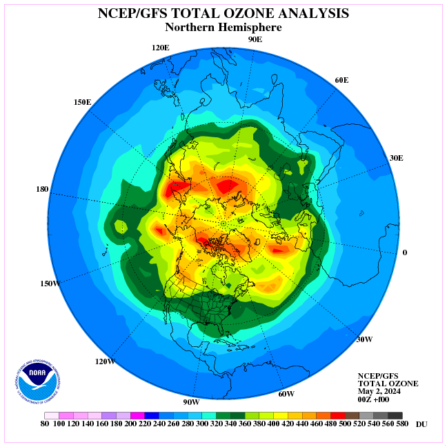
Forecast of the stratospheric polar vortex.
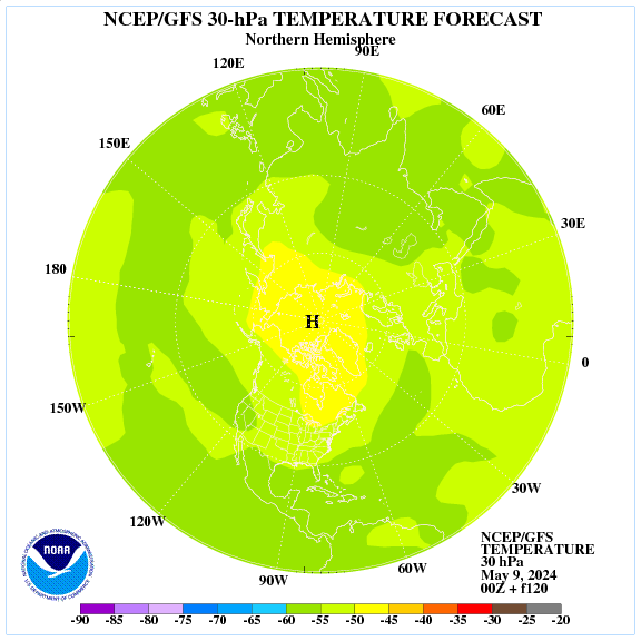
Model simulations cover the 2002-2010 period for which ionization rates from the AIMOS dataset and atmospheric composition observations from MIPAS are available. Results show that during geomagnetically active periods MEE significantly increase the amount of NOy and HOx in the polar winter mesosphere, in addition to other particles and sources, resulting in local ozone decreases of up to 35%. These changes are followed by an intensification of the polar night jet, as well as mesospheric warming and stratospheric cooling.
https://www.sciencedirect.com/science/article/pii/S1364682616301080
On the bright side, today is the day of the earliest sunset time. Starting tomorrow, sunset will be later each day. A sure sign that Spring is only 3 months away.
Wait, Tom; I thought that was at the solstice, around the 21st or 22nd of December?
Most people do but just check the charts. Most people also think that sunrise starts to come earlier the day after the solstice but it doesn’t. That comes later in January. However, the net gain in daylight minutes does start on the day after the solstice.
Specifically, which “charts” are you (Tom in Florida) are you using, and – more to the point of “changes in solar radiation received on the earth’s surface” which specific change are you referring to?
That is, the TOA solar radiation does reach a peak January 5 each year.
The rotational (23.45 axis tilt) length-of-day reaches a minimum December 21-22 each year – depending on Leap Year, time of the solstice, etc.
Are you using the “length of day” based on sunrise hour-minute-second change? If so, what part of the solar disk are using for sunrise and sunset? And, what air mass refraction definition are you working with for that level of accuracy?
Solar radiation on the earth’s surface starts with the assumed “TOA” value.
But total received energy from the sun is a function of latitude and day-of-year. All the rest are calculated FROM those two things. TOA radiation levels, length of exposure over the 24 hour “day”, angle of the sun above the horizon each minute of the day (and thus Air Mass), and thus attenuation through even a “perfect atmosphere”. Every surface’s albedo changes with one or more of these: solar elevation angle, with time-of-day, with day-of-year, and/or angle of the surface to the incoming rays.
The sun is 1/2 degree across (as is the moon of course), so changing the definition of “sunrise” or “sunset” matters when you could use “top of the disk goes below horizon” or “bottom of the disk touches the horizon” or “astronomical “middle of the refracted disk touches the horizon” – and all assume some perfect horizon with the observer, but seldom clarify at what height of eye is used.
This chart: https://www.timeanddate.com/sun/usa/sarasota
“Are you using the “length of day” based on sunrise hour-minute-second change?”
I didn’t say anything about length of day, I simply referred to the net change in daylight minutes, and that was from the chart.
You also said : “more to the point of “changes in solar radiation received on the earth’s surface” which specific change are you referring to?”
I didn’t refer to any solar radiation received in my comment. Where did you read that?
Then you go into some lengthy discourse on TOA peak radiation which has nothing to do with my comment. Then you go off into some cockeyed minutia about horizons and eye level. There is an official time of sunrise and sunset, it is as simple as that. If you want to complain about that go to the source and complain to them about how they calculate those times.
Yes, sunset here was about a minute or so later than only a few days ago. I have the exact times, but the horizon is ‘bumpy’.
I thought it might be a slight elevation in the land, but then I remembered about the earliest sunsets this many days before the solstice.
Correlations of global sea surface temperatures with the solar wind speed
‘Responses of sea-surface temperature to solar wind speed on
the seasonal timescale have been found, and in the North Atlantic
region in winter they resemble the North Atlantic Oscillation. At
the locations of the peak (negative) response in the North Atlantic
the SST decreases by approximately 1°C for 100 km s increase in solar wind speed.’
https://www.sciencedirect.com/science/article/pii/S1364682616300360
https://sci-hub.tw/10.1016/j.jastp.2016.02.010
Abstract
In this work we study links between low cloud anomalies (LCA) at middle latitudes of the Northern and Southern hemispheres and galactic cosmic ray (GCR) variations used as a proxy of solar variability on the decadal time scale. It was shown that these links are not direct, but realized through GCR/solar activity phenomena influence on the development of extratropical baric systems (cyclones and troughs) which form cloud field. The violation of a positive correlation between LCA and GCR intensity which was observed in the 1980s–1990s occurred simultaneously in the Northern and Southern hemispheres in the early 2000s and coincided with the sign reversal of GCR effects on troposphere circulation. It was suggested that a possible reason for the correlation reversal between cyclonic activity at middle latitudes and GCR fluxes is the change of the stratospheric polar vortex intensity which influences significantly the troposphere-stratosphere coupling. The evidences for a noticeable weakening of the polar vortices in the Arctic and Antarctic stratosphere in the early 2000s are provided. The results obtained suggest an important role of the polar vortex evolution as a reason for a temporal variability of solar activity effects on the lower atmosphere.
https://www.sciencedirect.com/science/article/pii/S1364682616300979
https://watchers.news/2015/06/09/cosmic-solar-radiation-as-the-cause-of-earthquakes-and-volcanic-eruptions/
In response to the very low solar activity a major explosive volcanic eruption or two will be taking place.
This is a very good article and it confirms that which I have long suspected, namely that climate change simply depends on the length of day/month/year…..and that this has not been constant over the history of earth, due to solar activity.
In any case: man made climate change does not exist , as a simple empirical experiment that I did will explain
(just click on my name to read my report on that).
I think I will bookmark this article in my report, is that OK?
I am pretty sure that looking at the variability of time is the right direction to look for any change in climate.
Perhaps a good summary of this post is:
Climate change is due to change in time.
….good slogan as well…
@ Andy May
“The apparent LOD variability at the same rate or close to the
solar cycles, as inferred from
the geomagnetic or the astronomical
observations, is unlikely to be a coincidence.
Alternatives for a viable mechanism could
be:
1. it is caused by solar activity
a) directly or b) indirectly.
2. solar cycles and the LOD oscillations have
a common origin.
Direct solar effect
1a)
After considering known physical properties
of the solar periodic oscillations (TSI cyclical
variability and intensity of the heliospheric
magnetic field at the Earth’s orbit), initial
calculations could not conclusively
demonstrate the existence of the viable
forcing due to insufficient energy available.
Similarly for
case 2
the known facts related to the generation of the solar
cycles and the changes in the Earth’s
rotation, do not revel existence of a clear
common external driving mechanism.
1b. Indirect solar effect
At the current state of knowledge, the most
realistic alternative is the indirect solar effect,
whereby a possible mechanism could be
postulated along line:
Solar activity – ocean & atmospheric temperatures –
oceanic and atmospheric circulation – angular momentum exchange
– Earth’s rate of rotation (LOD).
https://hal.archives-ouvertes.fr/hal-01071375v2/document
M. A. Vukcevic, thanks. Very few comments address the point of the post. Yours is welcomed. Yes, the integrating effect of the change in LOD is important. As Javier points out, daily (or monthly or yearly) changes in incoming or outgoing radiation probably don’t matter much. But, mechanisms for accumulating small changes in radiation at critical latitudes matter.
Details about measuring TSI are far less important to climate than long term accumulators and processes.
But, mechanisms for accumulating small changes in radiation at critical latitudes matter.
No, because the Earth is radiating away what comes in. No accumulation of small changes. A large change will matter because of the local effect of a growing ice sheet.
Leif,
“No, because the Earth is radiating away what comes in.”
This is total BS. The major difference between the Earth and a blackbody is the Earth’s surface can store a great deal of thermal energy for a very long period of time (over a thousand years). The average ocean temperature varies a lot over the Earth’s history, now it is very low, about 4C. It has been much higher in the past and the heat capacity of the oceans is huge. Further energy is stored in the ice caps and having ice caps on both poles is rare in the Earth’s history.
Ultimately, the energy absorbed on the Earth’s surface is radiated away, but the amount of time it is stored (especially in the oceans) is important, further the length of time required for the oceans to change temperature (system inertia) is important. As Javier notes, you are oversimplifying a complex problem.
Finally, sorry, I’m still not convinced the data supports your assertions, you are clearly overstepping the available TSI data in my opinion. And, my assumptions about the curves on your plot were correct.
The major difference between the Earth and a blackbody is the Earth’s surface can store a great deal of thermal energy for a very long period of time
Which also means that it takes a very long period of time to change that thermal energy, meaning that any short time variation [e.g. solar cycles] is completely washed out. And the cause of glaciations is the local cooling effect of accumulated snow and ice on landmasses. The oceans and their heat capacity have nothing to do with that.
Finally, sorry, I’m still not convinced the data supports your assertions, you are clearly overstepping the available TSI data in my opinion. And, my assumptions about the curves on your plot were correct.
That you are not convinced just shows your lack of understanding and knowledge. Your assumptions about the plot were wrong: no ‘raw’ data were shown. The plot showed the repeatability to within 0.1 W/m2 of TSI measurements by two different instruments. The absolute combined long-term uncertainty is below 0.5 W/m2 for the whole space age:
https://leif.org/research/Uncertainty-TSI-png
The sure mark of an activist is that he is never wrong and claims always to be correct [ my assumptions about the curves on your plot were correct ], even in the face of evidence to the contrary.
although I doubt you would even care to look.
Hold on dr S, Andy is correct.
Earth radiates from the surface, not from dept of the oceans.
It is indisputable fact that global temperature contains what appears to be an AMO component. It is also indisputable fact that warm surface waters due to increased salinity continuosly down well north-west of Iceland and any energy reminder is stored for about thousand or more years in the return leg of the ‘global conwayer belt’ . Part of that energy warms up ocean depths slowly perchlorating to the surface and part upwells south of the Aleutian archipelago, where it may re-radiate back, but both process have a millenal time constant.
Velocity and consequently volume of oceanic transport are dependent on the initial surface temperature, therefore they are time variant.
On the other hand, direct atmospheric circulation is subject to much shorter time constant measured in months or perhaps a bit longer.
As stated further above the logical conclusion is:
“Solar activity – ocean & atmospheric temperatures –
oceanic and atmospheric circulation – angular momentum exchange
– Earth’s rate of rotation (LOD).”
(posted from mobile/cell phone hence possible spelling etc errors)
Earth radiates from the surface, not from dept of the oceans.
The Earth warms at the surface and radiates [cools] from the surface.
That is where the balance between incoming and outgoing energy takes place.
Small changes in the incoming lead to similar small changes in the outgoing flux.
The notion that small changes get stored instead of leading to similar small changes in the outgoing is false.
Leif: “The notion that small changes get stored instead of leading to similar small changes in the outgoing is false.”
WR: Oceans do store energy. Look at the development of deep ocean temperatures:
Source: https://royalsocietypublishing.org/doi/full/10.1098/rsta.2012.0294
The change in stored energy causes different periods of glaciation:
http://wattsupwiththat.files.wordpress.com/2017/08/081217_1723_coolingdeep5.png
From: https://wattsupwiththat.com/2017/08/13/cooling-deep-oceans-and-the-earths-general-background-temperature/
Perhaps the quantity of stored energy is very small, but [at least] over longer time periods it matters.
Oceans do store energy
Of course they do, but they don’t vary much on time scales of years, decades, or even centuries, precisely because of their large heat capacity.
Do your think that the variation your plots show are caused by solar activity?
Leif: “Do your think that the variation your plots show are caused by solar activity?”
WR: Interesting question.
I read about the increasing luminosity of the Sun: estimated at 1% rise in a hundred million years. Quite a bit of warming. Looking at the graphics above, this did not result in rising surface temperatures during the last 100 million years: on the contrary, surface temperatures (that followed deep ocean temperatures) went down. On the time scale of millions of years other systems than the Sun’s irradiance showed to be dominant.
The total H2O temperature stabilizing system keeps temperatures within limits around what I called the General Background Temperature (see link above). The colder, the wider the limits, as is shown for our cold Quaternary period.
The H2O cooling/warming system (warming for the part that is caused by absorption of radiation by water vapor) reacts on any (!) change in temperature. Whatever the reason.
The temperature variation in the plots shown are dominated (!) by other factors (plate tectonics and their consequences). But this does not exclude influences by changes in the Sun’s irradiation during those periods, nor influences on smaller time scales. Not knowing all mechanisms involved I follow (from some distance) the discussions.
For now, given the complexity of the Earth’s climate systems, a linear result for changes in the Sun’s irradiance is not easy to see, which however does not exclude influences. On a time scale of century’s, millennia and in case we will have fully reliable data for those and longer periods we will know more.
But the present search for mechanisms is interesting. We don’t know what we are going to find.
a linear result for changes in the Sun’s irradiance is not easy to see
When changes are small they are all linear. If they are not easy to see it simply means that they are not significant, otherwise we would see them.
The large changes are due to astronomical changes of Earth’s ‘orientation parameters’ coupled with favorable distributions of landmasses, and at times helped along by extremes of CO2. None of this is of any interest for the current debate [food fight] about contemporary forcings and ‘global warming’.
EXACTLY – it is the long term accumulators and processes which so many can not grasp.
Nice article Javier. I want to address Leif’s SORCE opinions.
I spoke with Greg Kopp yesterday here at the AGU meeting, and he informed me SORCE has had 200ppm degradation since 2003, about 13ppm/year, or 0.2653 W/m2 in 15 years. He said it is far and away lower than the same parameter of the other instruments, and he gave some numbers that I didn’t write down.
I told him the following:
In my work I did long-term correlations of SORCE to F10.7 for the time of the last minimum, and in order to do the type solar-climate forecasting with TSI that I do, I have to know how well TSI is doing now (since 2014 when I started), and one metric I’ve used for this is the daily % difference between the current F10.7cm-SORCE TSI correlation and the prior correlation they had together during the last minimum.
Since 2014 the correlation difference exceeded 20% a few times, 18% some, 15% quite a bit, then under 10%, but now it’s down to 5-8% regularly, which only a few months ago is what I told Leif it would do going into the minimum, that is get closer to it’s prior correlation, meaning the current data is not so bad as Leif implies.
The annual approx 13ppm degradation equates to about 0.018 W/m2/year. How would this affect my SST forecasting method? My HadSST3 factor is 0.5C/W/yr based on the annual TSI change. So the degradation in one year, let’s say 2016, the year for which in Dec 2015 I had predicted SST3 would cool from the SWPC predicted drop in solar activity using this method, would affect my forecast to the tune of 0.009C for the year.
The HadSST3 high-end uncertainty is 0.03C, so the effect of the SORCE TSI degradation for the year 2016 on the performance of my TSI-SST3 sensitivity factor was over three times less than the actual SST3 uncertainty, in other words, it really didn’t matter, it was insignificant.
I’ve evaluated all the TSI data. They all operate within a very narrow range in cross-correlation with F10.7.
Further, Greg Kopp announced in his presentation that all the players in the TSI field have come together, including the RMIB, to produce a new CDR TSI record that everyone agrees on. After I return home I’ll be replacing the PMOD section of my work with this new composite data.
RMIB has trended higher than it should relative to other solar indices, moreso than SORCE, whereas PMOD was trending below the last solar minimum, so those two are out of the question. I have a nice graphic to show that but it’s on my other computer.
I talked to Bob Leamon and Scott McIntosh here, and earlier this year at the LASP Sun-Climate symposium. At the symposium I told Bob I had discovered the same thing they did in 2014, what I call a ‘cycle onset El Nino’, depicted in this graphic I made for my poster:
It’s getting late here in DC, and I have sessions to attend and posters to judge tomorrow before leaving, so I’ll wait to say more until Sat or Sunday.
Bob Weber:
However, what I have never seen corrected is the theoretical IPCC corrections need in their models for the reported TSI changes between 1988 and today.
Thus, everything the IPCC-CAGW models predict are based strictly on the radiation models they use.
In 1988, everybody “knew” TSI = 1372 watt/m^2. And the IPCC-Hansen CAGW models predicted +3 watts/m^2 based on a doubling of CO2, using a theoretical top of atmosphere radiation level of 1372 watts/m^2.
In 2005, the measured TSI was lowered (due to reported calibration errors in the sensors) to 1367 watts/m^2. And the IPCC-Hansen CAGW models predicted +3 watts/m^2 based on a doubling of CO2, using a theoretical top of atmosphere radiation level of 1367 watts/m^2.
In 2010, the measured TSI was reduced again to its latest value of 1362 watts/m^2 by the solar community. And the IPCC-Hansen CAGW models predicted +3 watts/m^2 based on a doubling of CO2, using a theoretical top of atmosphere radiation level of 1362 watts/m^2.
OK, fine. Their solar measurement business, not mine.
If the actual radiation emitted from the sun has not changed, which is what Lief has claimed has happened, then the value used in the computers for CAGW prediction MUST change as well, right? But the earth’s physical systems have NOT changed during the interval (except CO2 levels) so the predicted end result of increasing CO2 MUST change as well, right? That is, if their calculations were correct in 1988 for 1372 watts/^2, then using today’s radiation input of 1362 watts/M^2 , those same calculations MUST show a loss of energy of 10 watts/m^2 in received radiation for the next 80 years, and a resulting cooling effect over the next 100 years of 7 watts/M^2.
But the REPORTED TSI has been lowered 10 watts/m^2 – three times the calculated total influence of man’s release of CO2 – and three times the reported theoretical influence of CO2 has been “kept” at 3 watts/m^2 per doubling by the IPCC. Which tells me that their computer calculations have NOTHING to do with the actual radiation received from the sun, but only what they want reported out due to CO2 changing.
those same calculations MUST show a loss of energy of 10 watts/m^2 in received radiation for the next 80 years, and a resulting cooling effect over the next 100 years of 7 watts/M^2.
The cooling effect of 7 [or 10] W/m2 is about a third of a degree, but since we deal with anomalies that would be invisible as the base level would change by the same amount.
I spoke with Greg Kopp yesterday here at the AGU meeting, and he informed me SORCE has had 200ppm degradation since 2003, about 13ppm/year, or 0.2653 W/m2 in 15 years
The problem with SORCE is not that they have had too much degradation. In fact SORCE, measures MORE than expected [from RMIB and the SATIRE model and F10.7], so they have overcorrected for degradation.
The principal investigator [Tom Woods] agree with me. Here is an email exchange about this:
Leif Svalgaard
Sat, Apr 28, 6:36 AM
to Tom
Hi Tom,
I read with interest your newest paper on SSI, TSI trends and want to draw attention to my earlier analysis, that I presented at HAO:
http://www.leif.org/research/EUV-F107-and-TSI-CDR-HAO.pdf
I found a 22 ppm uncorrected trend.
============
Tom Woods
Sat, Apr 28, 11:41 AM
to leif@leif.org
Hi Leif,
Indeed – now there are 3 analyses that have found similar trend for the SORCE TSI record.
Greg Kopp may not update SORCE TIM data product though, at least not until there is more overlap with the new TSIS-1 TIM observations.
Tom Woods
===============
The consensus TSI have been promised for a couple of years now, but nothing has been released [as far as I know]. Greg is pussyfooting around the issue.
Further, Greg Kopp announced in his presentation that all the players in the TSI field have come together, including the RMIB, to produce a new CDR TSI record that everyone agrees on


A preliminary version may be found on Greg’s website https://spot.colorado.edu/~koppg/TSI/#TSI_data_record
Unfortunately it only goes up through 2015. Hopefully the final version will be up-to-date.
Anyway, the preliminary version goes a long way to resolve the calibration problem. I have for several years been telling Kopp that SORCE had a calibration problem [see e.g. Slide 61 of https://leif.org/research/EUV-F107-and-TSI-CDR-HAO.pdf ]. The ratio between the published SORCE TSI and the new preliminary version clearly shows that the original data is drifting upwards [i.e. overcorrected for degradation]:
The drift being of the order of 0.02 W/m^2 per year.
If I overplot the preliminary corrected values the fit to F10.7 and the sunspot number improves a lot [although 2015 still is anomalous (see slide 6 of https://leif.org/research/New-Group-Number-and-TSI.pdf )).
It is, of course, somewhat painful to admit that there was a problem, so Greg’s reluctance to come clean is understandable. Let us hope that the final consensus dataset will be out shortly. And let us hope that it is not extended back in time using the outdated Group Sunspot Number as time-varying ‘background’.
‘I leave for another day how the Moon produces some of the most abrupt cyclical climate change events of the past.’
I cannot wait for that!! Hope it will be soon?
Amazing is it not? It is the sun, the moon and most probably all the planets that are the cause of climate change….
Philip Mulholland says:
The direction of flow rule for the northern hemisphere is that if you stand with your back to the cold airmass, then the jet stream above you will be flowing from right to left. While this typically means an eastward airflow aloft, it is also possible, particularly in late winter, to have a westward flowing Arctic jet.
Henry says
Interesting choice of words. It was the same choice of words that Joseph used, but he went predicting the coming of the [dry] eastern wind
{click on my name to read my report]
indeed, by my calculations, drought time coming up, every 87 years, i.e. just about now, possibly starting 2019.
similar to dust bowl drought (1932-1939)
Henry
I always prefer to use toward because it unambiguously defines a direction of motion.
Hence a westward current flows towards the west.
By contrast a westerly wind is a wind coming from the west. The opportunities for confusion arising from using what is essentially a naval convention, useful for the time of sailing ships, means that I prefer to state the down-flow direction, hence my use of the ward suffix.
Philip
I am sure your choice of words is correct.
I was merely thinking about Joseph who was quite specific in his prediction that the change of direction of wind to the east that would bring [too] much heat and dryness.
Obviously there was no major ‘miracle’ in the story of Joseph because of the specifics. Most probably, the prison was on the Nile and Joseph was also in charge of observing the height of the Nile, whilst at the same time someone in the same office was also looking at the direction of the wind. Somehow, Joseph must have had access to these records and when he heard the dream of the Pharao he just put 2 and 2 together?
Remember that from our deliberations here about natural climate change all of us should be able to predict what will happen in the near future?
Can you?
If yes, what are your predictions?
@Leif
I like the science that has been posed here, namely that ‘climate change’ is due to change in time.
That would fit in with most theories, would it not? I mean you and I know there is no man made climate change. (click on my name to read my report on that).
But now how to explain that the sea water level here was at one stage 30 meters higher than what it is today? Can you give me a simple answer to that question?
Another question that I would like to ask you/anyone: as the sun burns up [for a million years or more] and as the earth cools down [for a million years or more] would you not naturally expect a variation of the time of the [earth] year, compared to the time of the [earth] year we have at the moment> due to the change in gravity??
Let me have your thoughts on that idea.
Great exploratory article Javier. I agree with your thesis that: “the efficiency of the poleward heat transport determines how much energy the planet retains, not the amount of CO2 in the atmosphere, which has a much smaller effect. ”
I did a search on the words ‘poleward heat transport’. Looks like all the commentators, with the exception of Macca, failed to appreciate the importance of this fundamental proposition.
The atmosphere rotates in the same direction as the earth but, at the winter pole it rotates much faster, atmospheric drag acting to speed up the rotation of the Earth so reducing the length of day.
You confirm this point when you write: From November to January the Earth accelerates to ~ 0.2 ms-day (ΔLOD changes by -0.2 ms). Then it decelerates by nearly the same amount by April. Afterwards it accelerates to ~ 1 ms-day by July (ΔLOD change of -1 ms), before decelerating back to the initial value by the next November. The average amplitude is ~ 0.35 ms, but the NH winter component is much smaller than the SH winter component (see figure 1, inset).From November to January the Earth accelerates to ~ 0.2 ms-day (ΔLOD changes by -0.2 ms). Then it decelerates by nearly the same amount by April. Afterwards it accelerates to ~ 1 ms-day by July (ΔLOD change of -1 ms), before decelerating back to the initial value by the next November. The average amplitude is ~ 0.35 ms, but the NH winter component is much smaller than the SH winter component (see figure 1, inset).
However, I think the motive force is electromagnetic in nature rather than being driven by ‘a need to transport heat’ as you suggest.
It has long been known that there is a correlation between the aa index of geomagnetic activity and the ‘Arctic Oscillation’, a measure of the differential in atmospheric pressure that determines whether the warm westerlies or the cold polar easterlies prevail in the mid latitudes.
What we experience as the ‘temperature of the day’ is the temperature of the air on that day. It simply depends on where the air comes from.
All this concern and irrelevant chatter about ‘total solar irradiance’ is a complete waste of time. There are more influential forces at work. People who insist on introducing irrelevancies should get short shrift. The word ‘malevolent’ springs to mind.
Phillip Mulholland’s contributions are apt.
Incidentally, notice the dominance of the southern hemisphere in determining LOD. The ocean is dominant in mid to high latitudes. The only landmass, Antarctica is located at the pole where air pressure reaches a global peak in mid-winter. On the margins of Antarctica atmospheric pressure is always at a resounding planetary low. The zone of low surface pressure surrounding the Antarctic continent expands markedly in winter and begins to affect mid and low latitudes where cold conditions tend to persist until November at which time the Arctic circulation kicks in with a vengeance.
The oscillations of the planetary winds that determine the rate and extent of heat transfer from warm to cold places is the essence of weather and climate. Climate studies have to start by appreciating this reality and endeavouring to explain the changes that occur on short and long-time scales. It’s the electromagnetic environment of the Earth in space that needs to be appreciated.
If one wants to understand the forces at work look at the southern hemisphere. All that land in the northern hemisphere complicates the issue. The highest surface pressures occur not in the Arctic but in Siberia.
Sorry, but I didn’t make the time to read all the comments.
This oceanography paper posted at Judith Curry’s site assesses the cause recent variation of North Atlantic Ocean circulation:
https://agupubs.onlinelibrary.wiley.com/doi/abs/10.1029/2018GL080474
Their study comes down on the side of internal variability, not external forcing.
All internal variation is due to external forces.
Salvatore says
All internal variation is due to external forces.
HENRY SAYS
funny thing that happened to me today:
A storm was brewing and I decided to have a quick swim before the rain…
…lying on my back as I looked up in the clouds I saw a fuzzy figure similar to that of God..
Amazing, is it not, to think that all good things ultimately depend on the weather!
May God bless you all!
https://breadonthewater.co.za/2017/02/20/if-god-exists-why-cannot-we-see-him/