Guest essay by Alberto Zaragoza Comendador
Summary:
- Climate models with different sensitivities reproduce the historical temperature record just as well (or badly)
- An interpretation could be the historical temperature record cannot be used to estimate or constraint climate sensitivity. This would imply that either the historical record is too short, or the forcing it involves is too small.
- This interpretation would be wrong: the time period and forcing involved in the historical record are long/big enough for the climate models’ sensitivity to emerge clearly. In other words, climate models should not reproduce the same temperature changes across the historical record; high-sensitivity models should show more warming than low-sensitivity ones.
- What climate models actually suggest is that true long-term climate sensitivity will be very similar to the sensitivity one can infer from the historical record.
- Okay, so then why don’t climate models actually diverge when reproducing the historical record? Because the high-sensitivity models have less forcing and / or more heat going into the ocean. If the same forcing and ocean heat uptake levels were applied to all climate models then the divergence between models of different sensitivities would be obvious.
Can climate models be used to estimate real-world climate sensitivity?
When attempting to estimate how sensitive the Earth’s climate is to an increase in greenhouse gas concentrations, researchers often turn to climate models. These offer a wide range of estimates on how much the Earth might warm as a result of a doubling of CO2 concentrations – roughly from 2ºC to 5ºC. So, in order to narrow (i.e. constrain) these numbers, many researchers try to focus on some aspect of the world’s climate and rank models by how well they emulate it. The reasoning is that, if for instance high-sensitivity models do a better job of mimicking real-world cloud behaviour, then these same high-sensitivity models may be better at representing other aspects of the climate system – including climate sensitivity.
This method is technically known as the emergent constraints approach. While there is in principle nothing wrong with trying it, a person who is new to the topic may be wondering why researchers don’t simply look at the most obvious constraint: temperature itself. The point of estimating climate sensitivity is to know how much the atmosphere will warm for a given increase in greenhouse gas concentrations (or radiative forcing to be more precise). In fewer words, we want to know future warming; doesn’t it make sense to look at how well the models have performed representing past warming?
The answer is that it makes sense but is not feasible, because models of widely varying sensitivities tend to reproduce the same temperature increases since the start of the observational record (∼1850). See this open-access paper and go to figure 3.

Models grouped into high- and low-sensitivity categories produce very similar amounts of warming until the present. Furthermore, the CMIP5 modeling groups knew the exam’s questions beforehand, so to speak, up to 2005; temperatures modelled before that year are not a forecast but a hindcast. And it’s around 2005 that a divergence starts to appear between high- and low-sensitivity models.
In short, you cannot use the historical temperature record to know which model is more accurate. Does that mean we don’t have enough data yet, or does it mean something else?
Man-made radiative forcing is already big enough for models to diverge according to their sensitivity
Look at the previous figure. The left panel shows temperature changes by the year 2100 under RCP 2.6, a scenario in which radiative forcing by the end of the century is 2.6 w/m2 above the baseline… and though I cannot find the exact definition of this baseline anywhere, I know it’s the figure around 1750 or 1850. As I’ll explain below, the exact baseline doesn’t matter much.
Clearly, 2.6w/m2 is enough for models to diverge; the temperature projections of low- and high-sensitivity models are separated by more than 0.5ºC. So how long will it take us to get to the RCP2.6 scenario? It turns out we’re already there. From the recent Lewis & Curry paper (hereinafter LC18), figure 2:

(The actual numbers can be found in the above link. Download the zip and open the AR5_Forc.new.csv file)
Total anthropogenic forcing as of 2016 was 2.82w/m2. LC18 use 1750 as a baseline, but using 1850 (if that’s the baseline the RCP scenarios use) would only reduce this figure by 0.1w/m2. In any case, current man-made radiative forcing is about as high as by the end of the RCP 2.6 scenario, or even higher.
Now, to be fair there is some divergence in current (2018) modelled temperatures under the RCP2.6 scenario, but there was virtually none by the end of the hindcast period, 2005. And by then, forcing was already 2.2w/m2 (again from an 1850 baseline). The point is, in simulations in which a forcing of 2 or 2.5 w/m2 is applied by the end of the XXI century, the models diverge; in reproducing historical temperature changes with similar forcing levels, the models don’t diverge. May that be because the historical record, while having a big enough forcing, is too brief for the models’ sensitivities to reveal themselves?
(Some readers will also be wondering: maybe LC18’s estimate of real-world forcing is higher than the forcing applied in models’ historical simulations? There is some evidence that indeed that’s the case. But if models have a smaller forcing than LC18, they should show a divergence in the historical simulations).
The historical record is more than long enough for the transient sensitivity of climate models to be estimated
First, some definitions. Transient sensitivity is technically called transient climate response (TCR). The ‘colloquial’ description of TCR is the amount of warming that has happened by the time CO2 concentrations have doubled. Because CO2 concentrations in the real world haven’t yet doubled, and we haven’t reached the equivalent forcing level even when including other greenhouse gases, observational studies have to use some approximation or extrapolation. For example, imagine that between 1950 and 2010 temperatures increased by 1ºC. Imagine, for the sake of illustration, that forcing increased between these two years by 2w/m2. That would mean warming so far is 0.5ºC/w/m2. Since the forcing associated with a doubling of CO2 concentrations is about 3.7w/m2, extrapolating you’d get that the TCR is 3.7w/m2 * 0.5ºC/w/m2 = 1.85ºC.
(Actually, observational studies don’t pick a single year, because yearly temperature and forcing can vary drastically due to El Niño, volcanoes, etc. Instead they look at the difference between two period averages, say 1950-60 and 2000-2010. Sometimes they use regression over the whole of the time period covered).
The definition of TCR in the context of climate models is a bit more formal. First, for matters of consistency it’s usually estimated by increasing CO2 concentrations 1% each year, thus doubling concentrations by year 70. Models also have ‘internal variability’, so to get a better idea of the warming caused by this doubling of CO2, what scientists actually calculate is the average temperature over years 60-80 of the simulation.
While this process may sound very artificial, there is evidence that climate models have virtually the same TCR whether driven by the 1%-a-year simulation or by the forcings of a historical simulation (see LC18, supplementary information, section S3). In any case, the main point is that estimating TCR in climate models takes about 70 years. Not hundreds.
(Wait. Did you the forcings applied in historical simulations by climate models are known? Actually, no – for a lot of models they are not known, which is why in order to estimate their sensitivity we have to resort to other kind of simulations).
More definitions of climate sensitivity
The acronym ECS has been used for different things over time so let’s back up a bit. First, the basic definition of equilibrium climate sensitivity is the eventual warming caused by a doubling of CO2.
Let’s say you double CO2 concentrations over 70 years. By the time concentrations have doubled, you measure temperature and thus calculate TCR. Supposing temperatures have increased 1.5ºC, then that’s the TCR.
But the planet will keep warming even if CO2 concentrations remain constant from that point on, because the climate system will be out of balance (i.e. the Earth will be taking in more energy than it’s releasing; that’s why the ocean is gaining heat). The process by which a body regains energy equilibrium is by increasing its release of heat, which happens when it gets hotter. Roughly speaking, an rise in ocean temperatures does not increase the energy release of the Earth because the ocean does not radiate to space; an increase of energy release requires a rise of air temperatures.
So if the Earth is in an energy imbalance, air temperature will keep rising until said imbalance reaches approximately zero, i.e. until the climate is in equilibrium: neither gaining nor losing heat, on the net. Let me emphasize: approximately zero. Everybody knows that the climate is never in complete equilibrium – and we couldn’t measure that even if it was, so it’s an irrelevant point. What matters is, how long does that take for the energy imbalance to get down to, let’s say, 0.1w/m2?
If climate model simulations are right, thousands of years! That’s a long time to wait – even in computer simulations. As a result, climate models are almost never run to equilibrium – it takes up too much computer power and time. Instead, the models’ equilibrium sensitivity has to be extrapolated from shorter simulations.
Here comes a complication. Continuing the previous example, let’s suppose upon doubling CO2 the planet has warmed by 1.5ºC, but there’s still an imbalance of 0.74w/m2. You can conceptualize it like this: out of the 3.7w/m2 of forcing that a doubling of CO2 involves, 2.96w/m2 have warmed the atmosphere while 0.74w/m2 has warmed the ocean. Thus, there is a ‘remaining’ forcing of 0.74w/m2 that has not yet acted to increase air temperature. Yes, physically that’s butchering the details, but I just want to get the concept across. What does the ‘remaining’ 0.74w/m2 mean, in terms of future atmospheric temperatures?
The standard formula used in many observational studies assumes that this remaining 0.74w/m2 will raise temperatures with the same efficacy as the previous 2.96w/m2. Following simple extrapolation, that means that if TCR = 1.5ºC, then ECS = 1.5 * (3.7 / 2.96) = 1.875ºC. Put other way, the ECS-to-TCR ratio would be 3.7 / 2.96 = 1.25.
Now, in climate models, that’s not exactly right. Usually, forcing applied at a later point in time raises temperatures more than if applied at an earlier point; in other words, their sensitivity increases over time. This is NOT to say simply that future temperatures will be greater than past temperatures; that will also happen if sensitivity is constant (or even declining!) over time. Rather, what it means is that future temperatures will be higher than if you simply extrapolated from past temperatures and forcings.
(The inverse of climate sensitivity is the feedback parameter λ. If you read a paper and it mentions ‘declining feedback parameter’ or something similar, what it actually means is increasing sensitivity).
This raises a problem: if papers based on observations about historical temperatures and forcings get an ECS result that depends on an assumption, and climate models’ behaviour doesn’t follow that assumption, then maybe the difference in ECS between observations and models is due to different definitions, not a mistake of the models. This was the point raised by Kyle Armour in this paper (henceforth I’ll call it A17).
A17 came up with a method to calculate the equilibrium climate sensitivity that climate models ‘would’ get if one used the same assumption as papers based on observations. A17 called this measure ECS_infer, referring to sensitivity as ‘inferred’ from the historical record; other studies termed it ICS, referring to sensitivity as calculated over the ‘industrial’ era. Previously, to distinguish true long-term sensitivity (ECS) from the results of observational studies and comparable measures of model sensitivity, sometimes the term ‘effective’ climate sensitivity was used, being equivalent to both ICS and ECS_infer. Finally, LC18 uses ECS_hist to refer to the same concept. I find ECS_hist more intuitive than the other denominations so I’ll stick with it.
LC18 took A17’s measure of ECS_hist, and added two more methods of measuring the same thing. Their three measurements are very similar (correlations among them are between 0.95 and 0.99). The ‘main’ ECS_hist result in LC18 is the average of the three methods.
Going back to the previous example, if the forcing caused by a doubling of CO2 concentrations is 3.7w/m2 and by the time CO2 concentrations have doubled there is still an imbalance of 0.74w/m2, then 1.25 is not the ECS-to-TCR ratio. Rather, 1.25 is the ECS_hist-to-TCR ratio. And the ECS-to-TCR ratio will be unknown, though climate models suggest higher.
Now, that’s a lot of mumbo jumbo. Surely at this point you’re wondering where I am going with all this discussion?
If you know a model’s TCR, you mostly know its ECS
In the previous section we saw that climate models have both an ECS (the warming that will take place over thousands of simulation years) and an ECS_hist (an estimate of how much they would warm if their climate sensitivity remained constant over time, as observational studies of climate sensitivity assume). LC18 provide, apart from the three measures of model ECS_hist and their average, one measure of model ECS; this data is available for 31 climate models. The actual numbers are in the ECStoICS.csv file; to make the following two plots I added the TCR values, taken from their table S2.
As you can see, TCR tells you pretty much all you need to calculate a model’s ECS_hist. For brevity I only post the plot showing TCR vs the mean of the ECS_hist estimates, but in the three cases correlation (r) is above 0.9.

There is the aforementioned caveat, that maybe ECS_hist is not a good measure because it differs from ECS. We can skip the ECS-to-ECS_hist step by directly comparing TCR with ECS. The relationship not so strong, but even there correlation is 0.74. Which is to say: more than half of the variance (0.74^2 = 0.55) in model ECS is explained by their TCR. This is remarkable: remember that ECS is designed to estimate temperature changes over thousands of years, whereas TCR looks at temperature changes over 70 years (and through a different method).

Differences between ECS and ECS_hist will likely be small
So, if the models are right, then true long-term climate sensitivity (ECS) will be higher than what can be estimated from the historical record (ECS_hist). In LC18 the mean difference between both measures is 12% (median 9%). Put other way, the ECS-to-ECS_hist ratio is above 1.
LC18 suggest one reason to be skeptical of the difference between both measures is that models with a high ECS_hist also tend to have a bigger increase when going from ECS_hist to ECS; in other words, if real-world ECS_hist is low, then the real-world difference between ECS_hist and ECS might be small as well. But this association is surprisingly weak: correlation (r) between ECS_hist and the ECS-to-ECS_hist ratio is 0.13, and statistically it’s nowhere near significance (p-value = 0.47).

Now, if ECS is indeed higher (or simply different) from ECS_hist, why could that be? Going back to the example of a doubling in CO2 concentrations, imagine that, by the time concentrations have doubled, the climate is already almost in equilibrium, with an imbalance of 0.2w/m2. In such a case, TCR will be very similar to ECS_hist… and, since only 0.2w/m2 of forcing can still warm the Earth, there is little possibility for deviations. It doesn’t matter much if the remaining 0.2w/m2 has a different efficacy than the previous 3.5w/m2, because the effect on long-term temperatures will be tiny anyway.
By contrast, imagine that by the time CO2 concentrations have doubled there is still an imbalance of 3.5w/m2. You could visualize this as: out of 3.7w/m2 of CO2 forcing, only 0.2w/m2 has actually warmed the atmosphere; the other 3.5w/m2 have gone into the ocean and so haven’t affected air temperatures yet. In such a scenario, ECS_hist would indeed be a very poor measure, because there’s so much extrapolation! You’d be using the effects of 0.2w/m2 to predict what would happen with the next 3.5w/m2.
In short: my thesis is that the closer TCR and ECS_hist are, the more reliable ECS_hist will be, in terms of being close to ECS.
In more words: if the ECS_hist-to-TCR ratio is low, then the ECS-to-ECS_hist ratio will also be low. If the energy imbalance is small as a proportion of forcing, then long-term climate sensitivity (ECS) will be very similar to the sensitivity that can be inferred from the historical record (ECS_hist).
Here I have plotted, from LC18, each models’ ECS_hist-to-TCR ratio and their correspondent ECS-to-ECS_hist ratio. The relationship is quite strong (r = 0.42, p-value = 0.019). I calculated three more ECS_hist-to-TCR ratios, one with each of the independent ECS_hist measures, and in all cases the correlation with the ECS-to-ECS_hist ratio is about 0.4

The question is: where on that plot would the real world be? Of course we cannot know the real world’s ECS-to-ECS_hist ratio, but according to LC18 its ECS_hist-to-TCR ratio is 1.25, below that of any climate model. This suggests that, if indeed the real-world ECS is higher than the ECS_hist, i.e. higher than the result obtained from observations of the historical record, the difference is likely to be minimal.
The reason climate models don’t diverge in the historical record: more sensitive models have less forcing and more heat going into the ocean
This is the part of the article I know the least about, so I’m mostly just going to point you to this paper by Stephen Schwartz and others. They look at 24 climate models and report their climate sensitivity and a combined measure of forcing and ocean heat uptake. Why combined?
Remember that the puzzle described at the beginning of the article was, why do climate models with differing sensitivities reproduce similar temperature changes over time? This could happen for two reasons. One is that high-sensitivity models have less forcing. The other is that high-sensitivity models have more heat going into the ocean, i.e. more forcing which has not yet warmed the atmosphere.
In the chart below, the global energy imbalance is called the ‘heating rate’ (roughly equivalent to ocean heat uptake), and denoted by N. Forcing is F. Thus, the amount of forcing that has affected the atmosphere is F minus N. And as you can see, models with high sensitivity (in the upper part of the chart) also have a smaller level of F minus N (they are on the left side).

Data on climate models’ historical forcing is hard to find, so I wouldn’t say Schwartz’s paper is definitive; I haven’t seen this kind of chart reproduced elsewhere. But so far it seems the best explanation.
PS: throughout the article I discuss how models ‘use’ forcing, or how forcing is or ‘applied’ to models. This is technically wrong, because radiative forcing is not prescribed; you cannot simply input a different forcing quantity and see how the model reacts. Rather, what is prescribed is the concentration of greenhouse gases and aerosols, and the physics for their interaction with each other, the clouds, sunlight, etc. So forcing levels ‘emerge’ from the models’ physics. That’s more accurate, but hard to use in a normal sentence.
Always assuming of course, that CO2 IS the significant driver of climate today that the models assume it is…
This reminds me of that old blues tune —
Well, C – O – 2 driver
Just see what you have a-done
Yeah, yeah yeah yeah C – O – 2 driver
See what you have a-done…
Used to sing it karaoke nite at the Climes, They Are A-Changin’ bar. Good times!
I solved the question of
“What is the CO2 ECS?”
in 1.25 seconds:
“No one knows”
No one knows if there
are feedbacks, and if there are,
no one knows if they are
positive or negative.
Unfortunately, people with science
degrees are very reluctant to answer
“I don’t know” or
“No one knows”,
to any question,
and too many
are willing to speculate
to get media attention
… and that’s why
most scientists
can’t be trusted.
Everyone does know, however,
that if all the warming since 1940
was caused by CO2***, then the TCS
is about 1, and that means CO2 is harmless!
*** Even the IPCC does not claim
100% of the warming after 1940 was
caused by CO2 — this is a worst case
assumption for CO2 TCS.
My climate blog:
http://www.elOnionBloggle.Blogspot.com
But that begs the question, has there been any warming since the 1940s? The honest answer to that is no one knows.
Locally, there’s been no warming and, since the 1890s, there’s been cooling. Slight cooling. Climate is local just as weather is local. Heating a gas in a bottle by shining light on it does not mean that shining light on gases in the open atmosphere will get heated. There’s much more going on, some of which shuffles energy without changing a sample’s internal kinetic energy.
How do you know if there has been warming or”cooling?
How do you measure it?
It isn’t so the models are all wrong.
Perhaps this is a bit off topic, but this thought occurred to me while reading the post.
Climate sensitivity discussions seem to treat the value implicitly as a constant. What if it’s not constant? What if it depends significantly on other variables of state in the climate system?
If that were true then one could discuss its value today…in a sense like a partial derivative. But the value a few hundred or thousands of years ago may have been different and that would certainly confound efforts at creating accurate models. And no, I don’t have any suggestions as to how the sensitivity might vary or what it might depend on. I was just thinking about it, wondering if this idea had occurred to others.
Here is a thought which crossed my mind last year. What if CO2’s function in this regard is that when the globe is in a Warm Period or shorter warming trend that CO2 enhances the warming due to its energetic response in handling outgoing energy in the atmosphere. As it absorbs and releases that extra energy a greater percentage is held within the system until escaping to space.
Then when the natural Cool Period or shorter cooling trend appears on the scene CO2 then acts to aid in the removal of energy in the atmosphere also due to its energetic ability to move energy around in the atmosphere. More works its way out to space faster as there is less energy in the system during the cool trend.
Your observation (your thought) is in essence what Christopher Monckton argues in the feedback assumptions used by the climate modelling community.
Well, the fact that sensitivity may vary according to other elements of the climate is another reason to use data from the thermometer rather than paleo record. We can’t know what will be the value of climate sensitivity in the year 2050, but surely it will be more similar to the year 2000 value than to that of the last ice age.
There is plenty of scientific rational to support the idea that the climate sensitivity of CO2 is zero. It does not matter whether it is a constant zero or a variable zero.
With all of the known negative feedback loops in the system, I’d put my money on ECS being a variable rather than a constant.
So temps have risen 1.8F and are going to rise for another 1000 years? Uh huh.
Is there a climate sensitivity?
https://chaamjamal.wordpress.com/2018/06/25/a-greenhouse-effect-of-atmospheric-co2/
Interesting site.
there is much to read.
And that is the problem for models. They model what they “know” and say that without climate sensitivity the models do not show recent changes, but climate sensitivity is as much of a fudge factor as just putting in “fudge factor” to make it all work. The fact that you can give a name to a possible solution does not mean that the possible solution is right.
Chaamjamal,
I think that you should have stated above that you make a case for ECS being a spurious correlation.
If there were a climate sensitivity we would not have needed a transient climate response to cumulative emissions TCRE
https://chaamjamal.wordpress.com/2018/05/06/tcr-transient-climate-response/
Chaamjamal wrote:
“The TCR is a specious metric because
it depends on the proportionality of temperature
with cumulative emissions.”
Chaamjamal — dat’s perfesser tawk !
It would be easier to understand if you
used simpler language.
For example, I might say:
It’s an unproven assumption that CO2 levels
control the average temperature, but the concepts
of TCR and ECS require jumping to that conclusion,
based only on simple lab experiments with CO2.
Would you agree with what I just said?
IMO the concept of climate sensitivity is flawed.
At the phase change in water heat input does NOT reflect in a temperature rise. Which may be described as ZERO sensitivity. Further any increase in heat input merely increases the rate of phase change.
This may be demonstrated in the kitchen kettle where at sea level it never boils above 100C and turning the heat up merely increases the rate of boiling.
I submit that this principle applies to the atmosphere albeit at different pressures and temperatures. The view that a small increase in heat input via CO2 entrapment will inevitably result in a temperature rise is thus flawed. All that will happen is that the water evaporation cycle will accelerate and offset the effect.
However water only exists as a percentage of the total atmosphere where matters of sensitivity are different. My main point being that the current concept is flawed unless this aspect of the behaviour of water is ignored.
All the CMIP 3 and CMIP 5 models with sensitivities above 2 K predict a detectable tropospheric hotspot as an emergent phenomenon of increasing CO2 forcing. The tropospheric hotspot is a emergent property manifestation of the fact that water vapor amplification is used (via subjective parameter tuning mostly) to get the 2xCO2 sensitivity above 2 K/doubling. As such, these models use copious amounts of water vapor forcing which has to be transported as latent heat vertically to the mid-troposphere in the tropics (where most convection occurs) and then condensing to release that energy as sensible heat in the cold air at 5-8 km up. The Hot Spot forms (in the models). It is not detected by either balloon radiosondes or via the the satellite AMSU records.
Observations since 1979 (satellite era of microwave sounding of the atmosphere) should tell the modellers that their ideas on water vapor amplification are wrong. They want to know then where the excess energy is going, if not increasing water vapor, that is a phase change.
The clear answer to the missing heat problem (If you accept the CO2 strong GHG forcing theory) is to assume a very slight warming of the deep oceans. It could only get there by increasing overturning circulation (speeding up the sinking of the surface water before it can release most of its heat at the polar oceans). That most climate models seem to project a decrease overturning points to even more fundamental model paradigm inconsistencies with nature.
But doesn’t it take somewhere in the order of a 1,000 years to overturn the deep ocean?
If this is sped up, what are we talking about? Eg., 900 years. 800 years, heck even 500 years? We cannot be talking about something that is measured in just say 50 years!
Much of the light from the Sun is thousands of years old (due to being trapped inside), but your skin still feels cooler almost immediately if you step into the shade.
“Overturning” is a lot different than “very slightly changing overall heat transport.” Since the hydrosphere is 300x more massive, the atmosphere can get pretty far out of overall equilibrium without the difference in average deep ocean temps even being measurable (assuming anyone ever starts measuring it).
Of course, another implication is that we can pour a lot more heat in there, limiting the heating of the atmosphere…
Alasdair,
Phase changes certainly complicate the situation of estimating energy retention using temperature as a proxy. In that may be a clue why long-term temperature increases approximate a step function rather than a noisy linear function.
Analyses like this, of what climate simulations do and why they do it, is interesting. But to me, in any case it makes no sense to even attempt to numerically simulate global climate with inputs of small effects such as 3.7 W/m^2. Why not? Because the “climate” is a composite result which includes heat fluxes thousands of times greater, in great numbers of events at small scale. For example, a one-inch-per-hour rate of rainfall implies an upward heat delivery of 16,000 W/m^2. Very common. Not so common but still observed are rates of 100,000 W/m^2 as strong convective weather produces rates of 6 inches per hour or more. So my estimate of climate sensitivity to rising concentrations of CO2 remains at zero, or very close to it, because weather tells us how the atmosphere responds to heat and water vapor. The power levels are way too high to allow CO2-induced warming to survive anywhere on earth. The heat engine rules.
“…rainfall implies an upward heat delivery of 16,000 W/m^2” I didn’t find anything searching, could you please expand on that in layman’s terms?
The 16,000 W/m^2 comes from the latent heat of water vapor released higher up as the condensed water falls down as rain. The calculation goes like this: 1 inch per hour / 12 inches per foot * 3.28^2 ft^2 per m^2 * 62.4 lbs/ ft^3 = 56 lbs per hour of water condensed. 56 lbs/hour * 970 BTU/lb latent heat = 54,000 BTU/hr. 54,000 BTU/hr / 3.412 BTU/watt-hr = 16,000 watts for the rainfall over 1 m^2 of area. I hope that helps.
Thanks David. So is that 1,360 W/m2 incoming and 16K W/m2 outgoing during a rain event? Is that energy lost, or just transferred elsewhere?
It would be heat transferred from the surface (evaporation) to the level of the atmosphere where the condensation/freezing occurs. So it is released to the mid & upper atmosphere where it can be radiated away to space.
Please take the 16,000 W/m^2 as an illustration of what is happening in magnitude. The actual heat fluxes are infinitely variable. The effects vary in altitude, all the way up to the tropopause. This is impressively exhibited by thunderstorms. Consider that the “greenhouse effect,” that is, the absorption of outgoing longwave radiation by the overlying atmosphere, diminishes with altitude. So yes, the energy is transferred elsewhere – upward – to where it escapes to space.
The 1,360 W/m^2 to which you refer is the total solar energy directed earthward at the top of the atmosphere directly facing the sun. Averaged over the entire surface of the earth, it is about 340 W/m^2. So this sets the inbound energy available to be absorbed or reflected. So even in comparison to these numbers, the atmosphere generates upward heat fluxes many times greater.
David
The rate would also vary with latitude?
Regards
The illustration of the high rates of heat flux implied by a specific rate of rainfall does not depend on latitude.
We need insufficient outflow data from the top of the atmosphere. CO2 is insulating all the activity including convective buildups and the stronger boundary layers. How much heat does the Earth lose all the time compared to that lost over regions of thunderstorm activity?
David,
One more thought to consider on the energy transport in a developing storm cloud. For example consider the LWIR emitting from the surface to a developing storm cloud. As the cloud begins to form from condensing moist air it becomes opaque to a degree and receives LWIR emitting at the surface temp that could be considerably warmer than the emitted LWIR from the cloud. A hot ground temp in excess of 100F and cloud at say 60F, that LWIR from the ground would be coming from a large ground surface area ahead of the developing storm cloud. Just consider a 45 degree angle outward ahead of the storm. It would amplify the amount of transported energy rising in the cloud and fuel its intensity. The absorption of this extra energy would be considerable and rising thru the convection in the cloud would ‘bypass’ the C02 emission altitude. Just a thought.
Storms? For a small storm to have a little bit of lightning in it it must reach the -20C height for that day.
True. to me this is liking saying that when I drain my bath, sea level rises. Probably true, but the effects is so small and the variability of everything else so great that it makes no measurable difference.
I’m replying here to my own comment to make sure there is no misunderstanding. To be clear, I am not implying that the high rates of heat flux in areas of precipitation would result in such high localized rates of LWIR outbound to space. Too much scattering. The key point is to acknowledge how easily and powerfully the atmosphere delivers heat up high, driven there by heat and water vapor itself, from down low. I regard Dr. Richard Lindzen’s views on how this all works to make good sense.
Thanks David
“In short, you cannot use the historical temperature record to know which model is more accurate. Does that mean we don’t have enough data yet, or does it mean something else?”
It means there’s no justification for adjusting past temps down….to show faster warming….to fit the narative
The models exactly extend that faster slope….and will never be right
For the benefit of those of us with short attention spans, articles longer than about 800 words should include abstracts.
Hell pochas94, most of my comments are more than 800 words 🙂
https://www.merriam-webster.com/dictionary/logorrhea
For the Radiative Green House Effect to function as advertised the surface of the earth must radiate as a 1.0 emissivity ideal black body.
But the non-radiative heat transfer processes, i.e. conduction, convection, advection, latent, of the atmospheric molecules render such ideal BB emission impossible, the effective surface emissivity being 0.16.
Without this ideal BB radiation the up/down/”back” GHG LWIR energy loop does not exist.
And carbon dioxide and the other GHGs have no role in the behavior of the climate.
According to Wikipedia:
Convection is usually the dominant form of heat transfer in liquids and gases.
http://en.wikipedia.org/wiki/Convective_heat_transfer
Nick the P Eng
No role? Have to disagree. GHG’s endow the atmosphere with the ability to cool via radiation. Without them the atmosphere would be much warmer.
At what concentration does CO2 have a net heating instead of net cooling effect? No idea. No one is talking about it. The radiative models and discussions forget about some of the things you mention. In the complete absence of GHG’s the surface heating (etc) continues, just with a great deal more incident radiation.
Question: is the back radiation intercepted by the surface more or less than the increase in direct insolation received, were the GHG’s absent? Where’s the inflection point? At what concentration does a GHG cool v.s. warm the atmosphere?
Sing it karaoke nite:
https://www.google.com/search?client=ms-android-samsung&biw=360&bih=288&ei=zCZXW5LpAujM6AT3tbmYBQ&q=the+Beatles+what+have+you++done+&oq=the+Beatles+what+have+you++done+&gs_l=mobile-gws-wiz-serp.
“….Earth might warm as a result of a doubling of CO2 concentrations – roughly from 2ºC to 5ºC.”,
or 1ºC, or 0.5ºC, or even 0ºC.
However, according to data relationship shown in HERE
the above strong correlation of R^2 = 0.8, if for some not yet defined reason is reflecting the causation (but that may not be necessarily so) indicates that there is following sensitivity:
Earth might warm about 1ºC as a result of an approximate fall in the Earth’s GMF 0.6-0.7µT (micro Tesla).
“result of an approximate fall in the Earth’s GMF 0.6-0.7µT (micro Tesla).”
That creates an arrow of causality from:
delta GMF to delta global T. that is: d(GMF) —> d(gT).
Why not instead:
(factor X) —> [delta GMF] and [delta gT] ?
you are correct, but not everyone may be familiar with even basic intricacies of calculus.
https://www.google.com/search?client=ms-android-samsung&ei=YitXW43rHqmHmwWAs6-QBw&q=mother+nature%27s+son+lyrics&oq=the+Beatles+born+a+poor+young+country+boy&gs_l=mobile-gws-wiz-serp.
Not to forget:
Live ist coupled system of nonlinear functions with chaotic behavior:
https://www.google.com/search?client=ms-android-samsung&ei=DSxXW57zM8WImwX_lYrICg&q=the+beatles+helter+skelter+lyrics&oq=the+Beatles+helter+skelter+&gs_l=mobile-gws-wiz-serp.
Climate sensitivity calculation requires a correct attribution of the warming observed. Otherwise the error is huge.
As Roy Spencer showed a few months ago if the warming attributed to anthropogenic causes is actually less, climate sensitivity drops like a stone.
http://www.drroyspencer.com/wp-content/uploads/Otto-vs-anthro-fraction-ECS.jpg
http://www.drroyspencer.com/2018/02/diagnosing-climate-sensitivity-assuming-some-natural-warming/
Therefore until we are capable of correctly attributing the origin of the observed warming discussing ECS is moot.
But you can only calculate ECS by making assumptions about the observed warming. This is why the models model assumptions and do not produce new information. If natural warming is 100% then sensitivity is zero. Of it is 0%, then it is a different number. No model can tell you that unless it can accurately predict temperature changes over a long period, and even then it might just be luck.
Running hundreds of models hundreds of times is a waste of everybody’s time.
“Running hundreds of models hundreds of times is a waste of everybody’s time.”
And, taxpayer’s money! To paraphrase an old joke about turtles, “It is assumptions all the way down.”
It shouldn’t take hundreds of years to estimate climate sensitivity
I’d say reasonable estimates have already been made (Spencer et al, Curry and several other groups). The eco-loons are stalling, and will continue stalling because it’s been apparent for some time that the sensitivity isn’t nearly high enough to serve their scare-mongering needs.
Beng
Measuring incoming versus outgoing IR and calculating a heating value is invalid, unless you clearly understand the mechanisms and the annual efficiency of those mechanisms that release the heat from the oceans.
It is assumed that those mechanisms are constantly 100% efficient. One in one out. Guess what, they are not.
Regards
6. The accuracy and precision of the data from past climate used for inputs to the models are far lower than generally acknowledged, and are too low for any useful output from the models.
7. The models do not reproduce known climate cycles, ENSO, ect., thus are unlikely to represent an accurate representation of reality.
A couple of points that could be added.
“But the planet will keep warming even if CO2 concentrations remain constant from that point on, because the climate system will be out of balance (i.e. the Earth will be taking in more energy than it’s releasing; that’s why the ocean is gaining heat).”
Disagree. SSTs are 3C higher than the surface on average, and energy form CO2 cant penetrate the ocean, thus there is no ‘ocean heat uptake’ energy from CO2 and it is not delayed from warming the troposphere.
Since we know the surface lag is about 3 hours, ie, peak sun + 3 hours = peak temperature, it is obvious the forcing from CO2 acts also in three hours.
TCR and ECS are one and the same thing. And the Taragonga / SAGE experiments dont show any different. For a start they used IR from clouds, very different to CO2 radiation, it penetrates water further and secondly the miniscule rise, what was it, 0.02 from over 100 watts, in SST would only cause the ocean to retain more visible derived energy.
Thus SAGE shows that if anything increased IR delays ocean heat loss!
“Roughly speaking, an rise in ocean temperatures does not increase the energy release of the Earth because the ocean does not radiate to space; an increase of energy release requires a rise of air temperatures.” Even after the sun goes down? “an increase of energy release requires a rise of air temperatures? Not necessarily. When the sun goes down the release of energy would help to slow down or maintain air temperature. By the way, how does Climate Model handle latent heat?
…It shouldn’t take hundreds of years to estimate climate sensitivity…
It had better if I’m going to make a good living out of it, and hand the job down to my children and grandchildren….
Alberto,
“Wait. Did you SAY the forcings …”?
The heat isn’t hiding in the oceans, we’d see it with thermal expansion.
Using the same rational of co2 levels for estimating global temperature in the recent past that doesn’t agree with anything else, proves that the models can’t forecast backwards as well. In my opinion, AGW fixed the co2 record to fix the temperature record.
Alberto,
You said, “This is technically wrong, because radiative forcing is not prescribed;…” I think that the modelers should strip off the input module(s) and test to see how the output varies with variation in forcing. When you have models that are too complex to mentally follow, one should simplify them and verify that they are working as expected. The above test would give more insight on just how forcing works in the models.
Build a simpler model. These huge models are no more accurate than a simple model. Stop trying to model the real Earth – which is simply impossible – and use first principles to show how simplified Earth would behave. Then people can look at that and udnerstand it and perhaps even agree with what is going on. From that you can move on if needs be to more complex modeling. But only after the fundamental ways the models work is agreed.
If you build a simple model, then people would understand it. You can’t hide BS in a model that people understand. You need complexity – the more the merrier – if you are trying to “make something happen that isn’t there.” You can build simulations that tell you something – that is exactly what these “models” are, simulations, and the based on the inherent beliefs of those writing the simulations. You can manage a real city by applying what you did in Sim City to it, but do not expect the same results. You can only “model” what you know. If you don’t have complete knowledge of the climate system – and no one does – you can only create simulations that may or may not be reflected in reality, for a minute, an hour, a day, a month or perhaps never.
The IPCC’s linearized definition of the ECS as the temperature change due to doubling CO2 obfuscates the underlying physics where the proper way to express a linear sensitivity is as the dimensionless ratio of a change in output power to the change in input power, where the output is defined as the surface whose temperature we care about (top of the oceans and bits of land that poke through). By this measure, the sensitivity is trivially calculated as the dimensionless constant 1.61, where each W/m^2 of input forcing results in 1.61 W/m^2 of output emissions. This metric is largely independent of the temperature. i.e. linear in the power domain, and the data supports this unambiguously. The green line below is the SB equation for a constant emissivity of 0.62 = 1/1.61 and it’s clear that even the monthly averages from satellite data relating the surface temperature to the emissions of the planet above that part of the surface (the small red dots) matches SB with e=0.62 almost exactly. The larger dots are 3 decade averages for each point on the surface being measured and matches the physics even more precisely and comprises undeniable evidence that the ECS is far less than being claimed by the IPCC.
http://www.palisad.com/co2/tp/fig1.png
If you must calculate the change in output temperature as a function of a change in the forcing input, you MUST account for the non linear relationship between power and temperature given by the Stefan-Boltzmann LAW. All you need to do is differentiate the SB equation relating the surface temperature to the planets emissions, where the only possible way to scale the T^4 relationship to power is with a linear scale factor called the emissivity. The T^4 dependence is immutable independent of whether you measure the radiant emissions consequential to the surface temperature at the surface, TOA or anywhere in between. Anyone who claims otherwise needs to articulate the specific law of physics that overrides this T^4 dependence. That being said, the sensitivity factor can be expressed EXACTLY as,
ECS = dTs/dPi = 1/(4oeTs^3)
where o is the SB constant, e is the ratio between the total emitted power (Po = 239 W/m^2) and the power emitted by the surface at its average temperature (390 W/m^2) (239/390 = 0.61) and Ts is the average temperature of the surface (288K). The EQUIVALENT emissivity, e, can also be expressed as (To/Ts)^4, where To is the radiant temperature of the planet as seen from space (255K). Replacing e with (To/Ts)^4 results in an expression for the ECS of,
ECS = Ts/(4oTo^4)
Note that in the steady state, oTo^4 is the same as the total power arriving from the Sun after reflection, Pi = Po = 239 W/m^2. We can rewrite the ECS equation as,
ECS = 0.25 Ts/Pi = 0.25 * 288/239 = 0.3K per W/m^2
which is below the lowest limit assumed by the IPCC’s bogus RCP scenarios of 0.4C per W/m^2.
Theory and data both unambiguously confirm an ECS less than the lower limit claimed by the IPCC.
Why is this still controversial?
The only potential argument to this analysis is that the boundary between the surface and atmosphere is more complicated than SB, of course, Trenberth’s energy balance disputes this. When you subtract out the return of latent heat and thermals from his ‘back radiation’ term, all that’s left is the power to replenish surface BB emissions. For this complexity to matter, you must quantify the effect that the energy of latent heat and thermals, plus their return to the surface has on the surface temperature and its emissions other than the effect they are already having on the average surface temperature and its emissions. Even if a second or third order effect could be identified, it would be no where near large enough to boost the sensitivity from 0.3 C W/m^2 to the nominal 0.8C per W/m^2 claimed by the IPCC and wouldn’t even be large enough to boost it to the 0.4C W/m^2 claimed lower bound.
Again, why is this still controversial?
I’ll tell you why, which is that the laws of physics do not support the kind of effect that the IPCC requires in order to justify its existence and that one of the most influential factors driving of an entrenched bureaucracy is self preservation.
Thanks, CO2. It’s worth studying your argument.
I’d be skeptical if I were you.
At https://wattsupwiththat.com/2016/09/07/how-climate-feedback-is-fubar/#comment-1856590 et seq. Jeff Peterson well and truly debunked the conservation-of-energy-based theory that co2isnotevil presented in the same-page head post, but co2isnotevil has persisted in it.
jhborn.
Peterson was clueless. His basic argument was that gain isn’t dimensionless because the inputs and outputs are not expressed in the same units. He fails to comprehend the fact that it’s because the inputs and outputs are not expressed in linearly related units that Bode’s analysis can’t be applied to the climate system in the way done by Hansen and Schlesinger which assumes that they are.
Bode requires strict linearity for his feedback analysis to be relevant. If the input is 1V and the output is 2V, the output will be 200V when the input is 100V, at least until the implicit power supply runs out of volts and the amplifier starts to clip, goes non linear and Bode’s analysis no longer applies. The missing implicit power supply is another of Bode’s preconditions missing from the Hansen/Schlesinger mis-application of Bode, although this can be addressed analytically by applying COE between the input and output of the gain block, which Bode’s basic analysis specifically does not do as a simplification enabled by the assumption of powered gain (i.e more power comes out of the gain block than goes in to it).
BTW, nobody has been able to debunk Conservation Of Energy. I’ve asked many of you many times to debunk COE by explaining how 1 W/m^2 of forcing results in 3.3 W/m^2 of ‘feedback’ which when added to the W/m^2 of forcing is sufficient to offset the 4.3 W/m^2 of additional emissions that would arise from the presumed nominal 0.8C increase. Forcing in and surface emissions out, both expressed in W/m^2 at least conforms to Bode’s linearity constraint that the input and output must be in linearly related units.
The real explanation preventing you from comprehending this argument is that expressing the sensitivity factor as 0.8C per W/m^2 sounds far more plausible than expressing it in the linearly related units of 4.3 W/m^2 of incremental surface emissions per W/m^2 of forcing (i.e. a gain of 4.3), even as both quantify the same amount of change.
The fact that all Joules are equivalent means that each of the 240 W/m^2 of forcing from the Sun must have the same effect as the next one. If each resulted in 4.3 W/m^2 of surface emissions, the surface emissions would correspond to a temperature close to the boiling point of water. Yet another test that falsifies the absurdly high sensitivity claimed by the IPCC.
You may try to arm this away by claiming a difference between the absolute gain of 1.6 (390 W/m^2 of surface emissions per 240 W/m^2 of solar forcing) and the incremental gain of 4.3 (4.3 W/m^2 from the next W/m^2) as presumed by the IPCC. This just tells me that you have no understanding of Bode’s linearity precondition that requires constant gain, independent of the amount of input. In other words, the absolute gain and the incremental gain must be the same.
You may also try to arm this away by claiming that all 240 W/m^2 of solar input are subject to ‘additional’ amplification and this is all bundled into the incremental effect from the next W/m^2. Not withstanding the fact that this also violates the linearity precondition, this is exactly what is happening and is the origin of the 3.7 W/m^2 of equivalent solar forcing said to arise from doubling CO2. In other words, doubling CO2 keeping solar forcing constant is EQUIVALENT to 3.7 W/m^2 more solar forcing keeping CO2 concentrations constant. This still can’t explain how 3.7 W/m^2 of EQUIVALENT forcing are amplified into the 16.4 W/m^2 of input to the surface required to offset the increased emissions from a surface temperature increase of 3C.
WUWT is a great site, and it does a good job of keeping new content coming. Most of it, though, is of the look-what-stupid-thing-alarmists-just-said type. When it comes to real technical discussions, its quality is uneven because the people who run it are unable to distinguish between real analysis and jibberish like Christopher Monckton’s posts and the “fubar” post I linked to previously.
Over the years I’ve dealt extensively with electrical engineers (“EEs”). As a group I think of them highly. I’ve said it before: some of the smartest people I’ve ever known were electrical engineers.
But here’s the problem: electrical engineering is hard. It’s so hard that not everyone who’s obtained a degree in it really understands everything they know about it. And that’s why we have co2isevil’s “fubar” argument.
The fubar argument is that the climate-feedback levels upon which high climate-sensitivity estimates are based would violate conservation of energy. The reason for this argument’s surprising persistence seems be its appeal to electrical engineers (“EEs”); it employs an electronics analogy. The climate system is not physically capable of such feedback levels, the argument goes, because the climate system lacks the internal power source that feedback-based electronic amplifiers include.
This theory’s focus is the linearized feedback equation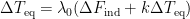 commonly used to describe the relationship that climate models exhibit between changes
  in equilibrium surface temperature and changes
  in temperature-independent “forcing.” That feedback equation is identical in form to the feedback equation
  that electrical engineers use to compute an electronic amplifier’s output voltage
  from its input voltage
  . Since amplifiers characterized by that equation require an internal power supply whereas the climate system has none, fubar-theory proponents contend that the equation can’t be correct for the climate system.
Proponents’ most-fundamental error, of course, is that little about an equation’s applicability to one system can validly be inferred from its applicability to a different system. The fact that power dissipation necessarily occurs in one type of system to which the equation applies, for example, tells us nothing about a different system, to which same-form equation
  applies: a rectangle can have area without consuming power.
Co2isnotevil goes on and on about linearity and conservation of energy, deluding himself into thinking the reason Patterson didn’t agree was a failure to recognize an energy-conservation violation, a failure based on confusion by the nonlinear relationship between temperature and radiation.
But the reason for the disagreement is simple arithmetic. Anyone who can do arithmetic can see that the surface emission’s exceeding the solar-radiation absorption does not violate conservation of energy. An example is here:
http://i68.tinypic.com/2qjejnr.jpg
jborn,
There you go, insulting me in a vain attempt to try and discredit my research. Moreover; you haven’t addressed anything I’ve said, except to claim I’m wrong, and they you support your claims with circular logic. You’ve definitely embraced the process of anti-science alarmism.
You don’t understand my argument if you think I mean that it’s a violation of COE that the surface is emitting more than it receives from the Sun. Clearly it does and the that you think I don’t think so tells me you’re grasping at straws to try and find a reason I could be wrong. Feel free to waste your time, but trying to understand what I’m saying would definitely be more enlightening then your current failure to understand.
It’s the 3.3 W/m^2 of feedback power arising from only 1 W/m^2 of forcing power and that’s required to support the 4.3 W/m^2 of incremental emissions arising from the claimed 0.8C increase that violates COE. The maximum amount of ‘feedback’ power that can arise from only 1 W/m^2 of forcing power is 1 W/m^2. In fact, the actual system only exhibits 600 mw of ‘feedback’ per W/m^2 of forcing and no where near the 3.3 W/m^2 required by the IPCC to support its insane ECS.
FYI, the 600 mw of feedback per W/m^2 of forcing does not violate COE as the origin of this power is easily identified as surface emissions emitted in the past and intercepted by GHG’s and/or clouds and ultimately returned to the surface.
You may be confused because you accept the possibility of a runaway GHG effect, which like the excess feedback power required by the IPCC to support its insane ECS, is only possible when an implicit, internal, infinite source of Joules is available to POWER the gain, as assumed by Bode in the first paragraph of his book. This book is the ONLY feedback related reference in either Hansen’s paper or the follow on paper by Schlesinger which together comprised the theoretical foundation for establishing the IPCC.
Please get your facts straight. The COE constraint omitted from climate science is between the input and output of the modeled gain block, not between the Sun and the surface. Bode omits this COE constraint too, as his precondition of an implicit, internal and infinite source of Joules powering the gain allows him to make this significant simplification. This simplification can’t apply to any model of the climate as the implicit, internal and infinite power supply is not there. It’s not the Sun, as the Sun is the forcing input, moreover; it’s not internal, implicit or infinite.
Co2isevil contends that I don’t understand his theory. Perhaps; it’s so full of non-sequiturs that re-assembling it into something intelligible is a challenge. But this isn’t my first experience with this guy, and his theory appears to be that it would violate energy conservation for feedback to exceed forcing without an internal power source.
Now, that theory requires a little interpretation because the way he uses the term feedback in that limitation is not entirely conventional. Feedback as co2isnotevil uses it does not mean a response to temperature, at least not solely. By that term he instead seems to refer to any excess of surface-absorbed radiation over the net radiation absorbed from the sun by the earth as a whole.
Recall that the earth’s effective radiation temperature is somewhere around 255 K, which means it’s radiating—and at equilibrium therefore absorbing from the sun—about . In contrast, the average surface temperature is around 288 K, meaning that it emits about
  : 1.6 times the radiation from the earth as a whole. Co2isnotevil referred to the difference between that ratio and unity as “feedback”:
Although he recognized that the difference does not by itself imply an energy-conservation violation, he seemed to believe that conservation of energy imposes a limit:
In that passage the “forcing” he referred to presumably was of the type caused by albedo changes. He criticized usual treatments (with some justification, in my view) for failing to distinguish between that type of forcing and forcing of the type in which CO2-concentration increases result. As to the latter, he seemed to impose a stricter limit:
Or maybe he was just being inconsistent.
In either case the misconception under which he seemed to be laboring can be appreciated by modeling the atmosphere as a lumped-parameter system. For the sake of simplicity we will assume that no convection or conduction occurs. Now, such a simplification makes the model differ quite significantly from the real atmosphere. For example, the resultant lapse rate is completely different. But it will serve to illustrate how energy is conserved despite (at least an apparent) power gain.
The diagram at http://i68.tinypic.com/2qjejnr.jpg depicts the model. It divides the atmosphere into two equal-optical-depth chunks, each of which is assumed for the sake of simplicity to allow all the radiation from the sun to pass through it to the earth’s surface. Each chunk also allows one-quarter of the radiation to pass through that reaches it from the surface or the other chunk. It absorbs and re-radiates the remainder, sending half up and half down.
For the sake of this energy-conservation discussion, that is, the radiation a chunk emits is assumed to equal the radiation it absorbs. Again, the hypothetical atmosphere therefore differs from the real-world atmosphere, in which not all energy transport is radiative. But all transport between the earth and space is indeed radiative, so the diagram adequately illustrates how an apparent power gain can result even in the absence of an internal power source.
Specifically, it shows that the same energy can be passed back and forth several times between the atmosphere and the surface before it escapes to outer space. So, even though the illustrated system has no internal power source, its surface emits 2.2 W/m^2 for every 1.0 W/m^2 it absorbs from the sun: the power gain is 2.2. The gain exceeds unity because energy that’s counted only once when it’s received from the sun is counted 1.2 more times at the surface before it escapes. (In the real earth system, that gain is more like 1.6, but the point here is that higher gains would not violate energy conservation.)
Now, our lumping the atmosphere’s opacity into discrete chunks could lead one erroneously to infer a gain limit. Specifically, whereas the illustrated transmittance of 1/4 resulted in a gain of 2.2, the gain approaches a limit of 3 as transmittance approaches zero. But that limit on gain is merely an artifact of the number of chunks: the limit increases as the (arbitrarily chosen) number of chunks does. From all that co2isnotevil’s comments reveal, he may have chosen one chunk instead of two, and that led him to conclude that energy conservation imposes a gain limit of 2.
His conclusion is consistent with his reasoning as follows. The radiation emitted from the surface equals the solar radiation
  plus the back radiation from the atmosphere. If we ignore what the atmosphere absorbs directly from the sun, we conclude that the maximum value of the atmospheric radiation
  is the surface radiation
  . But atmospheric radiation is isotropic, so only half of that can be returned to the surface. For zero transmittance, therefore, the resultant equilibrium feedback equation is
  , where we have expressed the system’s unity open-loop gain explicitly. (Note that what co2isnotevil refers to as “100\% positive feedback” is actually only 50\%.) This implies
  : the maximum possible gain is 2.
Again, though, that reasoning is erroneous because it doesn’t treat the atmosphere’s opacity as distributed. For a distributed-capacity model there is no limit on the apparent power gain; it can be shown that in the absence of convection and conduction the gain for an optical-depth- atmosphere is
  . Now, the real atmosphere has different optical depths at different wavelengths, and its lapse rate results from convection and adiabatic expansion, so that gain value doesn’t apply to the real world. But it does show that the fubar theory’s approach to imposing a feedback limit is too simplistic.
As described above, moreover, it suffers from a more-fundamental problem: it isn’t directed to the type of feedback on which high sensitivity estimates are based. As described above, the feedback it deals with is surface-radiation-caused back radiation (which in turn causes more surface radiation, etc.). In contrast, the feedback upon which claims of high sensitivity are based is a temperature-change-caused opacity increase (which in turn causes further temperature increase, etc.).
But I’ve already gone on too long. The point is that co2isnotevil’s theory is based on a lot of misapprehensions. It’s not worth your time.
jhborn,
Your misunderstandings are astounding, but I’m not surprised as the intention of all the misrepresentation, mis-characterization and obfuscation endemic throughout climate science is to have this exact effect. Don’t feel bad as far smarter people than you are even more confused.
Your idea that the same energy can be passed back and forth more than once is a kink in your logic because you fail to include the effects of delay. Each time energy is absorbed, DELAYED and returned to the surface, it’s added to different solar forcing then last time that energy was returned. In other words, each Joule absorbed by the atmosphere can be returned to the surface or emitted out into space once and only once. The same Joule absorbed by the atmosphere can not affect the surface at 2 different points in time or twice in the same instant of time.
Feedback in response to W/m^2 of forcing can ONLY be W/m^2 as you can not add degrees K to W/m^2 and use this as the input to gain block. The very definition of feedback is the fraction of the output added to the input before being amplified by the gain block. The idea of coefficients converting degrees K to W/m^2 to fake out temperature feedback is invalid as the ONLY equation that can convert between W/m^2 and degrees K is the Stefan-Boltzmann equation. This concept is one of the biggest deceptions in climate science. In effect, Schlesinger’s open loop gain is essentially the SB Equation which he explicitly undoes in the silly temperature feedback coefficient.
There can be no distinction between types of forcing. Joules are Joules, Watts are Watts and W/m^2 are W/m^2. The only legitimate source of forcing are the W/m^2 from the Sun. CO2 changes are a change to the system and the 3.7 W/m^2 of forcing said to arise represents the amount of net solar forcing at TOT/TOA that would be have the same effect on the surface temperature as doubling CO2.
You over-estimate the effect of the distributed opacity. Clouds are the primary mechanism that modulates opacity and emit energy in roughly equal proportions up and down, much like the photons in GHG absorption bands in the clear sky. You also seem to be ignoring the data which REQUIRES an average 50/50 split up/down of absorbed surface emissions in order to achieve balance.
I won’t expend any further effort on explaining basic physics and math to co2isnotevil. Before I leave, though, I will draw any lurkers’ attention to how people like him dupe readers. In response to clear refutations of their positions they make a lot of nonsense statements in the expectation that most readers won’t notice.
And in many cases most of them won’t. That’s because, although readers won’t really understand the arguments made by the co2isnotevils of the world, those arguments will sound like something readers have heard. The mere fact that co2isevil keeps mentioning Hendrik Bode doesn’t establish that he really understands Bode (he doesn’t) or that Bode is relevant to the conservation-of-energy question here (it isn’t), but citing Bode sounds erudite.
I spent a significant part of my career reviewing experts’ technical output, and I’ve learned not to believe purported experts who can’t give clear explanations. Yes, it happens all the time that one’s own limitations are the reason for his inability to understand a theory proponent’s explanations. But I know from experience that the reason for the difficulty is very often the proponent’s mistake. And that’s particularly likely when the proponent makes statements that are irrelevant to the issue, are completely unsupported, and/or are just flat wrong.
That’s the case here. The ultimate issue here is equilibrium climate sensitivity (“ECS”), which is the change in equilibrium temperature for a doubling of CO2 concentration. There are many good reasons to believe that ECS is low, but co2isnotevil’s “fubar” theory is not one of them. As I explained above, his rationale for why ECS can’t be high is his theory that energy conservation prohibits the surface from emitting more than twice the power it absorbs directly from the sun.
Here’s his reasoning:
He has given no authority for this novel theory, which common sense tells us is wrong. If the atmosphere can back-radiate energy it receives from the surface once, it can back-radiate that same energy again when the surface radiates it back to the atmosphere.
True, the earth’s surface radiates only about 1.6 times what the earth absorbs from the sun. But that results merely from the size of the earth’s atmosphere and that atmosphere’s opacity to infrared radiation; it is not required by energy conservation. This can be seen in the simple numerical example I provided at http://i68.tinypic.com/2qjejnr.jpg. From that example anyone who has a command of arithmetic can see that his assertion is wrong.
Specifically that diagram divides the earth into its surface, its lower atmosphere, and its upper atmosphere. The surface absorbs all the radiation from space (i.e., from the sun) as well as all the downward-directed radiation from the lower atmosphere together with all the downward-directed radiation from the upper atmosphere that the lower atmosphere does not absorb. The lower atmosphere absorbs ¾ of the radiation the surface emits and ¾ of the downward-directed radiation the upper atmosphere emits. The upper atmosphere absorbs ¾ of the remaining radiation from the surface and ¾ of the upward-directed radiation from the lower atmosphere. Space receives all the remaining upward-directed radiation from the surface, the lower atmosphere, and the upper atmosphere.
The radiant power the surface emits as a result exactly equals the total of the radiant power it receives from the sun, the lower atmosphere, and the upper atmosphere. The radiant power each atmosphere level emits exactly equals the total of the radiant power received by that atmosphere level from the other level and the surface. And the total that space receives from the other three components exactly equals the total radiation they receive from the sun.
So energy is conserved. Yet the surface radiates 2.2 times what it absorbs directly from the sun. And anyone who can do arithmetic can verify those facts; I’ve invoked no abstruse theories. And they could see it elsewhere in the solar system. My guess is that Venus’s surface emits ten or twenty times what Venus absorbs from the sun.
Unfortunately, c02isnotevil seemed unequal to the arithmetic. He objected to the example by saying, “You also seem to be ignoring the data which REQUIRES an average 50/50 split up/down of absorbed surface emissions in order to achieve balance.” But in that example both atmosphere layers emit exactly the same amounts in the upward direction as they do in the downward direction. Again, a fourth-grader could do the arithmetic to verify this. But co2isnotevil apparently couldn’t. As a consequence he made a statement that’s just flat wrong.
He also fixated on delay. But delay is irrelevant to a discussion of ECS. The E in ECS stands for “equilibrium.” That’s the operative word. Yes, delay affects how fast the system reaches equilibrium. But it has no effect on what equilibrium state is. For example, consider https://wattsupwiththat.com/2015/03/12/reflections-on-monckton-et-al-s-transience-fraction/. The delay-causing heat capacity C in its Fig. 3 transient diagram does not affect its Fig. 1 equilibrium diagram.
Co2isnotevil continues to spout irrelevance. He talks about “no distinction between different kinds of forcing” and asserts that I “overstate the effect of distributed opacity.” I won’t go into those statements’ errors here, but what the layman needs to ask himself is whether either proposition would refute the clear result I’ve set forth even if that proposition were true. The reason you can’t see the connection between those passages of his and my demonstration is that there isn’t any. If a theory’s proponent wants you to accept it, he should give you a clear explanation of why you should. I have. He hasn’t.
The rest of his response was mainly a dissertation on “converting degrees K to W/m^2 to fake out temperature feedback.” But my example had no degrees K: it dealt exclusively in W/m^2. So he again traffics in irrelevance.
Now, there’s a lot of hard-to-understand technical stuff out there, and none of us should dismiss something just because we can’t immediately understand it. But when someone like co2isnotevil repeatedly has failed to provide an intelligible reason for rejecting a clear, readily verifiable example such as mine, you are justified in concluding that he doesn’t know what he’s talking about.
Since Anthony Watts ran the fubar-theory post, though, many readers have been duped into believing it. Don’t be such a reader. Be skeptical.
jhborn,
Odd that you would deny time, but then again, many grasp at straws in their attempts to support the unsupportable. Allow me try and clarify how time disputes your position.
You claim that the same energy emitted by the surface and absorbed by the atmosphere can be returned to the surface more than once. As long as the energy of an absorbed photon is stored in the atmosphere, it’s still the same energy that was emitted by the surface. Once returned to the surface and re-emitted it’s no longer THE SAME ENERGY EMITTED BY THE SURFACE. When this energy returns to the surface, it accumulates with future solar forcing to offset future emissions and not the emissions that produced the photon in the first place, moreover; only past absorption can accumulate with current forcing and the available energy is limited to what was absorbed which is limited to what was emitted by the surface. The effect of time is so fundamental, it’s bizarre that you would deny it, but then again, to accept reality would be to admit that a lot of what you think you know is wrong.
You must understand that the average LTE response is an average calculated across moments in time. Energy returned at two different moments are different terms in the average and do not accumulate with each other, but average with each other. If 1 W/m^2 returned at t=0, another returned at t=1 and another at t=2, results in an average of (1 + 1 + 1) / 3 = 1, even it’s the same Joule!
Your denial of the linearity constraint and the implicit power supply required by Bode for the feedback analysis subverted by Hansen and Schlesinger is a clear signal that you are way out of your expertise, whatever that might be. I would school you on this, but it doesn’t seem like you would be receptive to the truth, as the truth would undermine so much of what you want to believe. I would encourage you to read and understand Bode’s book.
The surface definitely does not RADIATE 2.2 times what it receives from the Sun. The Sun delivers 240 W/m^2 to the system and the surface whose temperature we care about emits 390 W/m^2 at 288K, or only 1.6 times the solar forcing received by the system. Since we are considering only the LTE effect, solar energy absorbed by clouds is for all intents and purposes equivalent to solar energy absorbed by the oceans as the clouds are tightly and quickly coupled to the oceans by the hydro cycle. In LTE, clouds are simply a proxy for the oceans relative to their absorbed solar energy and emissions. The requirement for balance is fixed and cloud coverage simply adapts by modulating the ratio of cold (cloud tops) to hot (clear sky) as seen from space, until balance is achieved.
Your confusion may arise from Trenberth’s faulty energy balance where he improperly and arbitrarily conflates the energy transported by photons with the energy transported by matter. If you subtract out the non radiant return of latent heat and thermals from his bogus ‘back radiation’ term, all that’s left are the W/m^2 offsetting the SB emissions by the surface. Moreover; only energy transported by photons can leave the planet and participate in the radiative balance.
Why don’t you attempt to articulate how latent heat, thermals plus their return to the surface effects the average surface temperature and its corresponding BB emissions beyond the effect they’re already having on the average surface temperature and its corresponding emissions. Relative to the radiative balance and the resulting ECS, latent heat and thermals have a zero sum influence! Trenberth’s mistakes are yet another layer of obfuscation, misdirection and mis-characterization designed specifically to confuse. Clearly this seems to be working, but only temporarily, as subverting science is not a sustainable method to support what is precluded by the laws of physics.
BTW, the data supporting everything I say comes from Rossow’s ISCCP project at GISS. The FACT that the relationship between the surface temperature and the planet emissions corresponds to the SB equation with e=0.62 can ONLY arise from a 50/50 split of the roughly 75% of surface RADIANT emissions absorbed by GHG’s and clouds. Feel free to try and SUPPORT anything else. Just claiming something is not providing support, nor is citing alleged ‘peer reviewed’ papers. You must support your position with actual laws of physics.
http://www.palisad.com/co2/tp/fig1.png
Each little red dot is the monthly average temperature plotted against the planets emissions seen at TOA for each 2.5 degree latitudinal slice of the planet (i.e. constant solar forcing). The most significant difference between adjacent slices is solar forcing, thus the slope of the average relationship is the average sensitivity to a change in average solar forcing (i.e. the ECS). The larger dots are the 3 decade averages for each slice and matches the requirements of the theory even more precisely.
This is repeatable science, so unless you repeat this measurement and get different results, anything you say in a vain attempt to discount reality is meaningless. The results you need in order to be consistent with the IPCC must match the blue line in the above plot representing the nominal ‘linear’ sensitivity presumed by the IPCC. Clearly, the data is so far away from this, no amount of fudging will get the results you need.
Im no climate scientist but mu intuition tells me that measuring the net radiation st the coldest places on earth should clarify matters. The air is dry, presumably often cloud free, less noise in climate driver data. So what sensitivity do we see in the arctic and antarctic? Just go there and take meadutements and do the math. Climate Science sure is a lot easier when you dont understand how complicated it is.
The sensitivity has a 1/T^3 dependence on temperature, so as long as this is accounted for, it would be legitimate to use the sensitivity at the poles. One problem is that many sensitivity estimates come from polar data, like ice cores, and are then extrapolated to the planet as a whole without regard to the 1/T^3 dependence.
This is simply Trenberth’s lament of missing heat is hiding the oceans in a long-winded technical explanation.
Like Godzilla, the heat at 4.1 C rather than at 4.0 C will inevitably rise up and smack mankind.
Like Godzilla, it’s Total fiction, total bull. Total denial of the 2nd Law of Thermodynamics.
Seems to me that climate sensitivity is more of a human problem than an atmospheric one lately.
Folks are downright climate hypersensitive.
In the oil industry testing production models by history matching works very well.If it doesn’t fit its in the bin. The longer the history the better. However if the climate models or any models are built to mimic the past climate regardless. Then that indicates that the models are rubbish or worthless as a tool. Just a construct to fool people including it seems themselves also.
I think its daft to agonize over the individual model performance when that remains the case.
If they really knew what they were doing, there would be only one model but that is not the case. Because there are a plethora of models leeds one to the conclusion that a lot of guess work has been involved.
Initial radiametric calculations performed decades ago came up with a climate sensitivity for CO2 of 1.2 degrees C, not including feedbacks. A Japanese scientist pointed out that these calculations neglected the fact that a doubling of CO2 will cause a slight decrease in the dry lapse rate in the troposphere which a cooling effect. The slight decrease in the dry lapse rate will cause a decrease in the climate sensitivity of CO2 by more than a factor of twenty reducing the climate sensitivity of CO2 to a value less than .06 degrees C which is a rather trivial amount.
The AGW theory is that CO2 based warming will cause more H2O to enter the atmosphere which will cause even more warming because H2O is also a so called greenhouse gas. This positive feedback should amplify the global warming effect of CO2 but they are not sure by how much. What is completely ignored is that besides being the primary greenhouse gas, H2O is a primary coolant in the Earth’s atmosphere moving heat energy from the Earth’s surface which is primarily some form of H2O to where clouds form via the heat of vaporization. The net cooling effect of H2O is evidenced by the fact that the wet lapse rate is significantly less than the dry lapse rate. So instead of amplifying the warming effects of CO2, H2O retards the warming effects of CO2 which reduces the climate sensitivity of CO2 to an even smaller number.
The AGW conjecture depends upon the existence of a radiant greenhouse effect provided for by trace gases in the Earth’s atmosphere with LWIR absorption bands. This radiant greenhouse effect has not been observed in a real greenhouse, in the Earth’s atmosphere or anywhere else in the solar system. The radiant greenhouse effect is science fiction so hence the AGW conjecture is science fiction as well. Without the existence of a radiant greenhouse effect, the climate sensitivity of CO2 is zero.
I got bored with last half of the article ….. but the take home message is this:
IF … models of all kinds of sensitivities reproduce the same hindcast ….. THEN .. it goes to say that a model with an ECS of “0.00” is as accurate as any model created. Which means you cannot reject the null hypothesis that Climate Changes are completely natural.
There ya have it folks …. The ECS for CO2 is ZERO until someone proves otherwise!
“Climate models with different sensitivities reproduce the historical temperature record just as well (or badly)”
This isn’t at all surprising. Most – if not all – climate models are full of arbitrary parameters. Inevitably they will be adjusted in order to get the best fit with historical data. So, it doesn’t matter what the sensitivity of the models is: any divergence from historical data can be removed by adjusting the parameter values. It’s just a sophisticated form of curve fitting. It also means that the models have no forecasting ability at all.
This is the real climate change catastrophe: trillions of dollars squandered on the basis of climate models that have zero ability to forecast the future, and that are almost guaranteed to be wrong.
Chris
“By contrast, imagine that by the time CO2 concentrations have doubled there is still an imbalance of 3.5w/m2. You could visualize this as: out of 3.7w/m2 of CO2 forcing, only 0.2w/m2 has actually warmed the atmosphere; the other 3.5w/m2 have gone into the ocean and so haven’t affected air temperatures yet. In such a scenario, ECS_hist would indeed be a very poor measure, because there’s so much extrapolation! You’d be using the effects of 0.2w/m2 to predict what would happen with the next 3.5w/m2.”
Worse, we have little ability to predict how the atmospheric-hydrospheric relationship will evolve — we can barely even begin to measure it! The oceans are 99% of the climate system, and mostly occult, rendering implausible the whole idea of a climate system so completely dependent on a CO2 control knob that long-term global temps can be predicted as a function of human emissions.
Multi variable, non linear problem, so can’t reliably estimate future from past conditions.
One also cannot not assume that all variables have the same response to forcings/sensitivity, which is a key assumption of the IPCC=e.g. they assume climate sensitivity of the atmosphere is the same from solar as it is to C02. There is no reason it has to be this way and it is nothing more than academic convenience; eg solar variation may effect cloud cover, but C02 variation might not affect cloud cover.
Basic idea is that temperature observations helps, but non linearity and outsize effects from small changes in variables renders reliable estimates of ECS low, judging purely from past response.
It is back words it should be CO2’S sensitivity to the climate.
This is all an exercise which will soon no longer be necessary as CO2 concentrations will start to slow in reaction to the cooling environment. As the global temperatures, and overall sea surface temperatures continue to fall the CO2 /climate sensitivity issue should fade away, along with AGW theory and all it’s nonsense..
The reason for overall surface oceanic temperatures cooling is due to the prolonged minimum solar activity and the weak TSI, but in particular UV wave lengths which penetrate the surface ocean waters to depths of 50 meters.
As for EL NINO weak at best, but what is really important if one is expecting at a minimum a climatic shift, if not a climate regime change are the overall ocean sea surface temperatures and in particular the North Atlantic , both which are trending down and should continue to trend down in response to very weak solar activity.
All solar activity moderated by a weakening geo magnetic field which will compound the solar effects. Both being in sync.
I expect a slight up tick in albedo due to an increase in explosive volcanic activity and an increase in global cloud/snow coverage all tied to very low solar activity.
The other point here is that what is prescribed is not only the concentration of greenhouse gases and aerosols, but the hypothetical physics for their interaction with each other, the clouds, sunlight, etc.
So forcing levels ‘emerge’ from the modellers’ hypothetical physics, which are basically Feynman’s guesses, which prove no laws so are pseudo science by definition.
Modellers also also exclude factors they don’t like, by simply denying they’re large or variable enough, w/o having proven that. Examples are the true variability of plant response to CO2 , and Cosmic rays and CLOUDS vs water vapour as positive feedback. Not quite, Mr Mann. BTW the actual sensitivity of plants to CO2 in growth, aborption and reproduction is well known, direct and substantial, the opposite of modellers absolute science denying assertions in their model assumptions. Ask any commercial grower.
Finally the actual sensitivity is 0.8 in 288 degrees for a 120pp in 280ppm CO2 rise over 140 years, and diminishing logarithmically with concentration, even if it was true, all change was from CO2, and the tropospere was warming as GHE advertised. But it isn’t.
The heat isn’t lost, it isn’t being created.
That’s not a lot of sensitivity. 0.006:1, 0.6%, and cause in fact uncertain.