Guest essay by Thomas P. Sheahen
We all learned in elementary school that “you can’t divide by zero.” But what happens when you divide by a number very close to zero, a small fraction? The quotient shoots way up to a very large value.
Pick any number. If you divide 27 by 1, you get 27. If you divide 27 by 1/10, you get 270. Divide 27 by 1/1000 and you get 27,000. And so on. Any such division exercise blows up to a huge result as the denominator gets closer and closer to zero.
There are several indices being cited these days that get people’s attention, because of the big numbers displayed. But the reality is that those big numbers come entirely from having very small denominators when calculating a ratio. Three prominent examples of this mathematical artifact are: the feedback effect in global warming models; the “Global Warming Potential”; and the “Happy Planet Index.” Each of these is afflicted by the enormous distortion that results when a denominator is small.
A. The “Happy Planet Index” is the easiest to explain: It is used to compare different countries, and is formed by the combination of
(a x b x c) / d.
In this equation,
a = well-being “How satisfied the residents of each country feel with life overall” (based on a Gallup poll)
b = Life expectancy
c = Inequalities of outcomes. (“the inequalities between people within a country in terms of how long they live, and how happy they feel, based on the distribution in each country’s life expectancy and well-being data”)
d = Ecological Footprint (“the average impact that each resident of a country places on the environment, based on data prepared by the Global Footprint Network.”)
How do the assorted countries come out? Using this index, Costa Rica with a score of 44.7 is number 1; Mexico with a score of 40.7 is number 2; Bangladesh with a score of 38.4 is number 8; Venezuela with a score of 33.6 is 29; and the USA with a score of 20.7 is number 108 — out of 140 countries considered.
Beyond such obvious questions as “Why are so many people from Mexico coming to the USA while almost none are going the other way?”, it is instructive to look at the role of the denominator (factor d) in arriving at those numerical index values.
Any country with a very low level of economic activity will have a low value of “Ecological Footprint.” Uninhabited jungle or barren desert score very low in that category. With a very small number for factor (d), it doesn’t make a whole lot of difference what the numbers for (a), (b) and (c) are — the tiny denominator guarantees that the quotient will be large. Hence the large index reported for some truly squalid places.
The underlying reason that the “Happy Planet Index” is so misleading is because it includes division by a number that for some countries gets pretty close to zero.
B. The second example of this effect is the parameter “Global Warming Potential,” which is used to compare the relative strength of assorted greenhouse gases.
The misuse of numbers here has led to all sorts of dreadful predictions about the need to do away with very minor trace gases like methane (CH4), N2O and others.
“Global Warming Potential” was first introduced in IPCC second assessment report, and later formalized by the IPCC in its Fourth Assessment Report of 2007 (AR-4). It is described in section 2.10.2 of the text by Working Group 1. To grasp what it means, it is first necessary to understand how molecules absorb and re-emit radiation.
Every gas absorbs radiation in certain spectral bands, and the more of a gas is present, the more it absorbs. Nitrogen (N2), 77% of the atmosphere, absorbs in the near-UV part of the spectrum, but not in the visible or infrared range. Water vapor (H2O) is a sufficiently strong absorber in the infrared that it causes the greenhouse effect and warms the Earth by over 30 C, making our planet much more habitable. In places where little water vapor is present, there is less absorption, less greenhouse effect, and it soon gets cold (think of nighttime in the desert).
Once a molecule absorbs a photon, it gains energy and goes into an excited state; until that energy is lost (via re-radiation or collisions), that molecule won’t absorb another photon. A consequence of this is that the total absorption by any gas gradually saturates as the amount of that gas increases. A tiny amount of a gas absorbs very effectively, but if the amount is doubled, the total absorption will be less than twice as much as at first; and similarly if doubled again and again. We say the absorption has logarithmic dependence on the concentration of the particular gas. The curve of how total absorption falls off varies according to the exponential function, exp (-X/A), where X is the amount of a gas present [typically expressed in parts per million, ppm], and A is a constant related to the physics of the molecule. Each gas will have a different value, denoted B, C, D, etc. Getting these numbers within + 15% is considered pretty good.
There is so much water vapor in the atmosphere (variable, above 10,000 ppm, or 1% in concentration) that its absorption is completely saturated, so there’s not much to discuss. By contrast, the gas CO2 is a steady value of about 400 ppm, and its absorption is about 98% saturated. That coincides with the coefficient A being roughly equivalent to 100 ppm.
This excursion into the physics of absorption pays off when we look at the mathematics that goes into calculating the “Global Warming Potential” (GWP) of a trace gas. GWP is defined in terms of the ratio of the slopes of the absorption curves for two gases: specifically, the slope for the gas of interest divided by the slope for carbon dioxide. The slope of any curve is the first derivative of that curve. Economists speak of the “marginal” change in a function. For a change of 1 ppm in the concentration, what is the change in the radiative efficiency?
At this point, it is crucial to observe that every other gas is compared to CO2 to determine its GWP value. In other words, whatever GWP value is determined for CO2, that value is re-set equal to 1, so that the calculation of GWP for a gas produces a number compared to CO2. The slope of the absorption curve for CO2 becomes the denominator of the calculation to find the GWP of every other gas.
Now let’s calculate that denominator: When the absorption function is exp (-X/A), it is a mathematical fact that the first derivative = [-1/A][exp(-X/A)]. In the case of CO2 concentration being 400 ppm, when A = 100 ppm, that slope is [-1/100][exp (-4)] = – 0.000183. That is one mighty flat curve, with an extremely gentle slope that is slightly negative.
Next, examine the gas that’s to be compared with CO2, and calculate the numerator:
It bears mentioning that the calculation of GWP also contains a factor related to the atmospheric lifetime of each gas; that is discussed in the appendix. Here we’ll concentrate on the change in absorption due to a small change in concentration. The slope of the absorption curve will be comparatively steep, because that molecule is at low concentration, able to catch all the photons that come its way.
To be numerically specific, consider methane (CH4), with an atmospheric concentration of about Y = 1.7 ppm; or N2O, at concentration Z = 0.3 ppm. Perhaps their numerical coefficients are B ~ 50 or C ~ 150; they won’t be terribly far from the value of A for CO2. Taking the first derivative gives [-1/B][exp{-Y/B)]. Look at this closely: with Y or Z so close to zero, the exponential factor will be approximately 1, so the derivative is just 1/B (or 1/C, etc.). Maybe that number is 1/50 or 1/150 – but it won’t be as small as 0.000183, the CO2 slope that appears in the denominator.
In fact, the denominator (the slope of the CO2 curve as it nears saturation) is guaranteed to be a factor of about [exp (-4)] smaller than the numerator — for the very simple reason that there is ~ 400 times as much CO2 present, and its job of absorbing photons is nearly all done.
When a normal-sized numerator is divided by a tiny denominator, the quotient blows up. The GWP for assorted gases come out to very large numbers, like 25 for CH4 and 300 for N2O. The atmospheric-lifetime factor swings some of these numbers around still further: some of the hydrofluorocarbons (trade name = Freon) have gigantic GWPs: HFC-134a, used in most auto air conditioners, winds up with GWP above 1,300. The IPCC suggests an error bracket of + 35% on these estimates. However, the reality is that every one of the GWPs calculated is enormously inflated due to division by the extremely small denominator associated with the slope of the CO2 absorption curve.
The calculation of GWP is not so much a warning about other gases, but rather an indictment of CO2, which (at 400 ppm) would not change its absorption perceptibly if CO2 concentration increased or decreased by 1 ppm.
C. The third example comes from the estimates of the “feedback effect” in computational models of global warming.
The term “Climate Sensitivity” expresses how much the temperature will rise if the greenhouse gas CO2 doubles in concentration. A relevant parameter in the calculation is “radiative forcing,” which can be treated either with or without feedback effects associated with water vapor in the atmosphere. Setting aside a lot of details, the “no feedback” case involves a factor l that characterizes the strength of the warming effect of CO2. But with feedback, that factor changes to [ l /(1 – bl)], where b is the sum of assorted feedback terms, such as reflection of radiation from clouds and other physical mechanisms; each of those is assigned a numerical quantity. The value of l tends to be around 0.3. The collected sum of the feedback terms is widely variable and hotly debated, but in the computational models used by the IPCC in prior years, the value of b tended to be about b = 2.8.
Notice that as là 1/3 and b à 3, the denominator à zero. For the particular case of l = 0.3 and b = 2.8, the denominator is 0.16 and the “feedback factor” becomes 6.25. It was that small denominator and consequent exaggerated feedback factor that increased the estimate of “Climate Sensitivity” from under 1 oC in the no-feedback case to alarmingly large estimates of temperature change. Some newspapers spoke of “11 oF increases in global temperatures.” Nobody paid attention to the numerical details.
In more recent years, the study of various positive and negative contributions to feedback improved, and the value of the sum b dropped to about 1, reducing the feedback factor to about 1.4. The value of the “Climate Sensitivity” estimated 30 years ago in the “Charney Report” was 3 oC + 1.5 oC. Today, the IPCC gingerly speaks of projected Climate Sensitivity being “near the lower end of the range.” That sobering revision can be traced to the change from a tiny denominator to a normal denominator.
The Take-Home lesson in all of this is to beware of tiny denominators.
Any numerical factor that is cranked out is increasingly meaningless as the denominator shrinks.
When some parameter (such as “Climate Sensitivity” or “Global Warming Potential” or “Happy Planet Index”) has built into it a small denominator, don’t believe it. Such parameters have no meaning or purpose other than generating alarm and headlines.
APPENDIX
Duration-Time Factor in “Global Warming Potential”
The “Global Warming Potential” (GWP) is not merely the ratio of the slopes of two similar curves at different selected points. There is also a factor that strives to account for the length of time a particular gas stays in the atmosphere. The idea is to integrate over a long interval of time and thus capture the total energy absorbed by a gas during its residence time in the atmosphere.
For methane, there is general agreement that the mean lifetime is 12 years. Unfortunately, for carbon dioxide there is no agreement at all; estimates range across 5 years to 200 years. It’s debatable whether to count the time for a CO2 molecule to enter a tree, or the lifetime of that tree. The IPCC does not settle this issue by choosing a single number for the CO2 lifetime; rather, in a footnote to table 2-14 of AR-4, it presents a formula for the response function to a pulse of CO2. That extremely obscure formula has 7 free parameters to fit data, as it tries to accommodate 3 different plausible lifetimes. This makes it nearly impossible for outsiders to discern what numerical value goes into the denominator of every GWP calculation. A plausible guess for the average lifetime of CO2 is 55 years, but 100 years is not implausible.
When it is too difficult to carry out an actual integral over data that is very uncertain and widely variable, the next best thing is to select one number for the lifetime and multiply by it. We thus obtain the simple form
GWP = __Slope (gas) x lifetime (gas)
Slope (CO2) x lifetime (CO2)
The guesswork involved in that will probably afflict both numerator and denominator is roughly the same way.
If we take 55 years as the lifetime of CO2, 12 years as the lifetime of CH4; and use 0.000183 as the slope in the denominator, and 1/B = 1/50 as the slope in the numerator, the numbers work out to GWP = 23.85 – a number close to 22, 24 and 25, each of which has sometimes been stated as the GWP of methane.
The same procedure can be used for N2O, for the Freons, for any other gas. The guesswork about lifetimes definitely enlarges the error brackets, but the really enormous factor that drives the calculated GWP numbers up is the extremely flat slope of the CO2 absorption curve (0.000183 in the example above). That is entirely due to the fact that the absorption by CO2 is very near saturation.
Get Willis onto this right away…he’s the master of measuring things that cannot be measured then performing amazing calculations based on that data!
Though, I’d have preferred the acknowledgement of the one, and only one, exception to the divide by zero rule, have been included.
0/0 = 1
Much like the “Apples and Oranges Comparison” exception.
When do apples equal oranges?
When there are none.
PTP
If I remember correctly my math teacher told me that 0/0 (and anything divided by 0) was “undefined. The reason for that is that division is actually determining how many times you can subtract the denominator from the numerator before you hit 0 [btw that is how computers divide-they can only add and subtract]. 8/4 is 2 because you can subtract 4 from 8 two times. Now, how many times can you subtract 0 from a number (including 0 itself) before you hit 0? An infinite amount. And in the the case of 0/0 any number you want from 0 to infinity. That is why it is undefined.
“0/0 = 1”
When I were a nipper my NaN told me something else …
My computer science profs said it was all the fault of those lazy mathematicians who have been so busy playing with prime numbers and block-chains that they still have not done their jobs of defining division by zero.
My cyber stored the result of 1/0 as indef (1777 xxxx xxxx xxxx xxxx), as I recall, but then give you a “core dump” only if you tried to use that result (which helped a veteran NASA engineer find a nasty bug involving having accidentally switched the numerator and divisor in his simulator).
And -1/0 gave nindef (6000 xxxx xxxx xxxx xxxx).
But it could also give positive and negative over-flow.
Some of ye olde Ill-Begotten Monstrosities would just deliver 0 as the result and romp on (which was a surprise to an architectural engineer in St. Louis), while the one at the state legislature would crash on the operation, giving a 4-lettter code like NaFN…which I’b better leave as it is.
Richard Patton:
When I first started working (many moons ago), we had an old mechanical calculator that did division by repeated subtraction. Since it was mechanical, it was rather slow and you could watch it chug away at a problem until it came up with an answer. If you set up a division by zero on it, it would gamely try to come up with an answer, but the result was that it would run forever or until it lost power, whichever came first.
It’s undefined because division by zero gives absurd results.
Suppose x=1
then x-1 = x^2-1
x-1 = (x+1)*(x-1)
divide both sides by x-1 and you get
(x/1)/(x-1) = (x+1)(x-1)/(x-1)
1= x+1
substituting back in x=1 and you’ve just ‘proved’
1=2
The error was that division by (x-1) =0/
0/0 is an invalid expression.
IIRR, George Gamow said 0/0 was indeterminate in a book I read in 1950.
Determining 0/0 is what calculus is all about. And calculus (with limiting values) makes perfect sense.
This article is silly. Small denominators aren’t themselves the problem. They just upscale the answer, and who is to say what scale is right. There are plenty of ways a ratio can give a bad answer. If you aren’t sure whether a denominator is positive or negative, that’s a problem.
@RicDre – my mother worked out of our home for a non-profit. She had a rented electro-mechanical calculator (I think it was made by Olivetti). Its designers had a linkage that locked the zero key when the division key was pressed, and didn’t unlock it until one of the other number keys was pressed. Division time was still fun, though, when a small denominator was used. Shook up everything in that part of the wood frame house we lived in; she never used it where we had glassed picture frames.
(When I was at the age where I was inquisitive, could use tools, and had no common sense, that calculator was kept well out of my reach…)
@Nick Stokes – part of calculus is, indeed, determining the limit of a dependent variable as an independent variable approaches a constant value (which may or may not be zero). So far, you are correct.
However… your normal penchant for obfuscation appears yet again. The choice of a denominator in whatever function you are examining is subject to abuse. Taking just the first example – “Happy Planet Index” – the researchers (whether deliberately or ignorantly, I will leave to the jury to decide) ensured that, through their choice of a denominator that is very large for advanced/capitalist nations and very small for primitive and/or socialist nations, the latter would receive an unwarranted advantage in the “index.”
This is called “bad science.” Or a different description, which would send this into moderation, and I might as well not waste Charles’s time.
“This is called “bad science.””
Well, I don’t think the “Happy Planet” index is science at all. But the fact that d is in the denominator is irrelevant. It would have the same effect in the numerator. It dominates because it has a broad range.
“This article is silly. Small denominators aren’t themselves the problem. They just upscale the answer, and who is to say what scale is right. There are plenty of ways a ratio can give a bad answer. If you aren’t sure whether a denominator is positive or negative, that’s a problem.”
Nick do you never tire of sophistry?
You don’t disprove the point the article discusses, just say there are plenty of problems – as if that somehow means one if those problems us not a problem.
A tiny denominator chosen arbitrarily is a problem. It gives a scale that makes no sense nd when a scale makes no sense we are entitled to say it is wrong.
It’s called numerical instability, in maths…
Marvelous piece.
+11
“…..400 times as much CO2 present, and its job of absorbing photons is nearly all done.”
And water vapor in the tropical troposphere is 3%. So 30000/410 = 73 times CO2. Not much left there for CO2 either.
Although the CO2 and H2O absorption spectra have a lot of overlap and water absorption dominates in the overlap regions, there is a region around the 4 micron wavelength that is not/poorly absorbed by H2O but is absorbed by CO2.http://clivebest.com/blog/wp-content/uploads/2010/01/595px-atmospheric_transmission.png
And what temperature corresponds to that wavelength (4 micron wavelength)?
Don K,
To Richard’s point,
that H2Owindow-CO2 absorption band is at 4.0-.4.2 microns. Using Wein’s Displacement law for 4.1 microns and an emissivity of 0.95, that corresponds to a radiating grey body at 457℃. Not a factor.
(btw as an aside, That CO2 4-micron strong absorption band is very close to Venus surface T of 462℃.)
Some more background for ya.
All of Earth’s climate is radiating IR from a Tmax ~ 319 K (hottest dry desert 115 F, sea level) to a Tmin = 205 K (top of troposphere). At 0.95 emissivity, that corresponds to 8.6 microns to 13.4 microns gray body IR radiators. Which is precisely where the water vapor window exists, confirming that it is the ocean water-vapor interface and water vapor IR absorption window in the troposphere that dominantly control Earth’s surface and tropospheric temperature profile.
The addition of the CO2 GHGE brings in slightly more IR absorption starting at ~12 micron, which is a -16℃ gray body radiator w/emissivity of 0.94. Assuming a warm ocean SST at 30℃ and the typical tropical moist adiabatic lapse rate of 5 km/K, then -15℃ to -20.0℃ temps are found in the tropical troposphere at 9 km to 10km altitude. So it is just below this altitude (~6km – 8 km) then where the GCM’s predict a tropical tropospheric hotspot should exist due to the GHG effect warming this region relatively faster than the surface under increasing GHG forcing.
In fact the CMIP3 model mean for the predicted hotspot/surface anomaly is a warming ratio of ~1.3 as CO2 increases.
Unfortunately for the CAGWers and their models, this hotspot is not observed in either the Satellite MSU data or the radiosonde (balloon) data set. The observed ratio is about 0.8, which informs us that the surface warming recorded by various data sets is not due to a GHE.
5 K/km is moist lapse rate, wrote it backwards. Typing without thinking, & going too fast.
I suggest that the reason there is no hotspot is that water rises, being lighter than dry air. The produces a form of vertical lenticular cloud where energy passes through with the location appearing static. Large energies are involved here on their way up to the cirrus clouds and beyond to space.
It is just the good old Rankine Cycle doing its stuff.
It would be better to say that the water rises on net because its fraction is moving faster. Fixed KE = 1/2 * m * v^2. For the ratio of mass 1 to 2 the velocity difference will be the square root of the ratio.
That said, water vapor is not necessarily all water monomers. Also the ideal gas relation is a limit relation given a set of conditions.
Gases are fully miscible, too.
Any mug knows that the people in Mexico are far happier than the people in the USA.
Which is why all Mexicans want to stay in Mexico and Donald Trump is having to build a wall to stop people from the USA from going to Mexico.
It is the “Happy Planet Index”, not the happy people index. Note that as the population of a country approaches zero the Happy Planet Index approaches infinity. So it fits right in to the anti-human radical-enviro narrative.
“It is the “Happy Planet Index”, not the happy people index. ”
Well said.
Some people don’t seem to have realized that.
Mexico? where drug gangs celebrate the Goddess of Death in rituals by cutting off heads from real people.
I have to print this out….so I can read it again
Thank you Dr. Sheahen!!
That’s wrong. Molecules have multiple energy states. The easiest to understand is rotational. A molecule can rotate at a certain base speed, or a little less than twice as fast, or a little less than three times as fast, etc. etc. The base speed is determined by the de Broglie wavelength. The molecule rotates at such speeds as will produce standing waves. Because only certain speeds work, they are called quantum states.
With the above in mind, a molecule could be hit by a photon and attain the first quantum state. It could then be hit by another photon and attain the second quantum state, and so forth. On the other hand, one photon with the correct energy would be sufficient to promote the molecule to any given energy state.
Why, you ask, is the frequency of the second rotational state less than twice the first? That’s because the molecular bonds stretch. The frequency change gives you a big clue about the strength of the atomic bonds.
Molecules tend to absorb energy selectively. That gives rise to absorption spectra. In any event, the energy state won’t be increased unless the photon has enough energy. The energy state could be increased by a photon that has excess energy. There is a strong preference for photons with exactly the right energy. That’s why CO2 absorbs energy only at certain wavelengths.
I must have read that automatically as “Once a molecule absorbs a photon of a particular wavelength…” You are quite correct. (However, I’m going to have to dig back into my references, is there a significant terrestrial emission wavelength corresponding to the transition from one excited state of CO2 to a higher one?)
Lifetime of CO2. I don’t grab it. CO2 exists a long as there is a chemical reaction which changes it to another molecule.
Just to expand the story a bit:
One small little CO2 Molecule is fumed out of a bio engine or a technical engine or a camp fire or out of a rotten leaf or out of the oceanic carbonic acid. So it life starts.
How long will you live, little CO2?
As the air is constantly moving, it will travel around and possibly hit a plant, which collects via photo synthesis it’s C, and leaves the O, which normally will pair with another O. So game over, litte CO2, R.I.P.
Or it will hit cold water and will be transformed into carbonic acid. Also here it’s life is finished.
Possibly it will be caught an bottled or pressed under the earth’s surface in a cave. Now in prison, no freedom, no dealing with IR radiation. But still alive, and eventually set free again, medddling again with IR radiation.
To discuss about lifetime makes no sense.
The questions are: How much CO2 is in the Air? Where does is come from? And what does it to the environment?.
What it does to the environment? It greens it, as you have described.
Johannes Herbst,
The alarmists are constantly warning us about what they think the future holds, and they claim that if we stopped producing anthropogenic CO2 tomorrow, we would still be left with a problem. Therefore, the real question to be asked (and answered) is “What if we should ban fossil fuels and immediately cease producing it? How long would it take for the atmosphere to revert to the pre-industrial levels of CO2?” Probably the best estimate for that comes from the C14 spike in the atmosphere created by above-ground nuclear tests. It certainly is no where near the 100,000 years some loon claimed in a comment with regard to a recent news article.
A thing that changed my worldview was when they tagged the water and CO2 in photosynthesis and found out that the oxygen gas produced always comes from the water’s oxygen atoms. The CO2 remains intact as part of the carbohydrate. It then gets realeased, still unbroken, when the carb, usually cellulose, rots and breaks down.
The fact that 1000 molecules of water transpire from a leaf, on average, to capture one CO2 molecule, also gets you thinking about the transfer of greenhouse gases and energy involved in the process, when you ask, “Where does the incoming energy go?”
On carbolic acid in the alkaline ocean, you need free hydrogen ions for the CO2 to react with. Water doesn’t react with CO2. Gasses dissolve in water. There is 52 times more CO2 in the ocean than in the atmosphere. I assume the other gases are present in that ratio too, as gases.
Also 44% of all the CO2 we emit never registers, so you can say 44% is instantly absorbed somewhere or disappears.
It’s so complicated, and that’s why all extreme calls have to be considered seriously in debate. No one knows. 200 years duration was chosen by the scaremongers because that means that once it is in the air, cooking, the cooking is then irreversible. If it was said to be a 5 year duration, then there is no fear, trillions and power for them.
CO2 is soluble in rainwater, which falls from the sky when Jupiter Pluvius commands it to.
There have been about 80 studies which say that the lifetime of CO2 is around 4 to 9 years. This all depends on whose figures you believe for annual recycling of CO2 between oceans and atmosphere. No one disputes that the atmosphere contains 800 gigatons of carbon at 410 ppm. Not too many people dispute the DOE figures of 90 gigatons/yr absorbing into oceans from atmosphere and 90 gigatons /yr absorbing into the atmosphere from the oceans . Based on these figures CO2 lifetime could not be more than 800/90 = 8.88 years. Other researchers give the figure as low as 3.9 years. You cannot have this much CO2 being recycled every year and have a long lifetime. IPCC figures of CO2 lifetimes are junk science.
This is obviously not drawn from one of those 80 studies.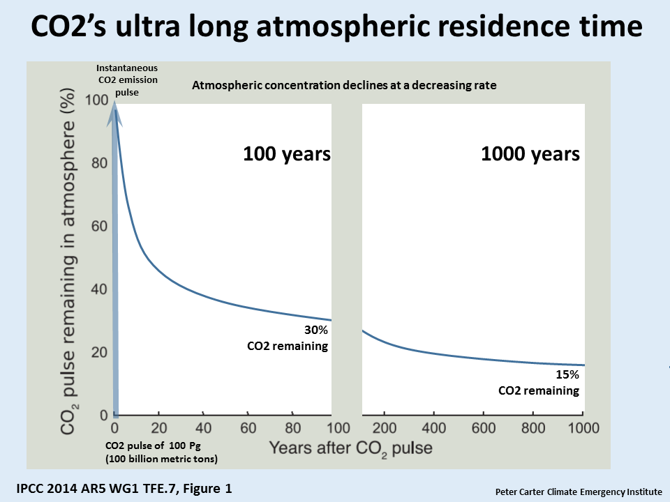
zazove, you are conflating two different times, atmospheric residence time and CO2 lifetime. See my comment elsewhere in this thread.
w.
I see. But do you see my point? That after a 1000 years (lets talk round numbers) you still have a sizable residue. Not: meh, its gone in 3.9, See, more junk science.
Interesting how that’s unremarkable but I need educating for being a conflater.
I guess thats how the effects of today’s emissions dont really peak for ten years or even centuries depending on the size of the pulse as this suggests: http://iopscience.iop.org/article/10.1088/1748-9326/10/3/031001
“Lifetime of CO2. I don’t grab it. …”
I think the rigorous term is “residence time (in the atmosphere) Eventually the CO2 molecule will end up in a carbonate (or bicarbonate) rock or will be incorporated into to an organic Carbon molecule, or something. Anyway, it eventually leaves the atmosphere.
So far as I can tell, this “lifetime” thing is a bogus value used to frighten the gullible. “OMG! That awful CO2 will stay around for 200 years! We better do something now or we are doomed!”
Things like conversion to carbonates or photosynthesis or dissolution in water are better expressed by a half-life than a lifetime since any particular molecule might be absorbed immediately or wait around for thousands of years. Not only that but I suspect the value is very dependent upon concentration. The half life will be less in a higher concentration. Lastly, these are not irreversible processes. The CO2 can be (and is) released again in every case by natural processes.
Some one needs to explain to me how this “lifetime” is any kind of meaningful measure.
This is a statement that absorption of light tails off because all the molecules are simultaneously in their excited state.
This is *not* the way it works.
Two parts:
1) Once a molecule is in it’s excited state, it will not absorb another photon. *TRUE*
(Nobody mention Raman spectroscopy, a 2 photon process)
2) This effect causes “saturation” *FALSE*
A wavelength is said to be saturated when all the radiation is absorbed, not the state of the absorbing molecule.
A thought experiment:
Consider an absorbance cell 5.00 cm long.
We fill the cell with some molecule such that 90% of the incoming light is absorbed in the first cm., and 10% of the light is transmitted to the second 1.00 cm. segment.
The second 1.00 cm. segment will absorb 90% of what is left.
Now our total absorption is 90% + 9% = 99%, so 1% if the initial radiation is transmitted to the third 1.00 cm. segment.
As before, the third segment absorbs 90% of what is left, or 0.9%
Total absorption is 90% + 9% + 0.9% = 99.9%.
This is the fundamental basis for the logarithmic response of increasing concentrations.
Note:
After the first 1.00 cm, 90% of the energy is taken up, so the system is largely defined, as the physics students shout with glee “To The First Order!”
After the second segment, 99% of the available energy is accounted for, so the system really is pretty well nailed down. After all, there is only 1% of the incident energy left to play with, no matter what happens next.
Note 2:
Beat on the system hard enough, and eventually you get the photons re-emitted, which causes the Beer-Lambert plot to roll over and go non-linear. So absorbance is *decreased* compared to the more usual (ideal) case.
Molecules have multiple excited states. simple explanation They can, and do absorb energy from multiple collisions. link A molecule can always be promoted to a higher energy state, unless it breaks apart.
Of course.
I should have specified *at that wavelength*.
Molecular absorption and Beer-Lambert *always* specifies at a single specified wavelength, one at a time.
We often take it for granted that this condition is understood.
Around here, you have to specify *everything*, and assume *nothing*.
Just after I hit the “post Comment” button, I realized I had not explicitly stated *at a single wavelength*.
From then on, it was just a matter of time.
Most of the time, what you say is true. I just stumbled across this paper. I’m still absorbing it. Things get interesting when you use a laser and get a much enhanced probability of multiple collisions.
@ commieBob:
I asked you *not* to mention Raman spectroscopy!
OK, formally they are not collecting spectra, they are blasting the molecules to bits.
But the two photon process is at the heart of the Raman process.
And giving the associated energy levels the full quantum mechanical mathematics treatment.
So what are they up to????
1) They mention important isotope selectivity. Hmmmmm.
2) Test molecules are sulfur hexaflouride and uranium hexaflouride (!!!)
Why would Los Alamos be interested in those things???
Better Living Through Chemistry
Thomas, this his seems to be a typo. Let me know what it should be and I’ll fix it. I think it means “approaches”, but …
Most interesting post …
w.
PS—you haven’t mentioned an associated problem, which is averages. When you average ratios, the ones with a small denominator dominate the result … and trends such as “change in A / change in B” are ratios.
It is mathematically illegal to average ratios save under two possible conditions: that they have the same denominators, or that they are expected to have the same value. This latter exception is permitted when replicating an experiment and one reasonably expects the result to be the same. You can average those results.
Where the numerators are the same and the denominators are different, use the Harmonic Mean to average. A special case formula is given for the averaging of two fractions (ratios).
We cannot say that having a small denominator has a greater effect on an average, it depends on the value of the numerator standing over the large denominator.
One thing I do not understand: “Saturation” of CO.
1. In normal air, CO2 absorbs one photon and transfers the energy by vibration contact to another neighboring air molecule, mostly oxygen or nitrogen. This changes the average temperature of the surrounding air a bit, so to speak. And that specific CO2 molecule can absorb another photon, and so forth.
2. All molecules of a certain amount of air at a certain height have about the same temperature and vibrate according to their temperature. This causes the greenhouse gas molecules to emit IR radiation in a random direction. And this continues as long the temp is above 0 Kelvin. And as the greenhouse molecules get constantly energy from other surrounding molecules, this will go on forever.
So in normal air, CO2 never gets saturated. It will be different at 100 km height, where the next neighboring molecule is far away.
Buuut. Say one brave CO2 molecule, far away from other comrade gets hit by a photon, which gives it some energy and makes it “hotter”. So the next photon comes around, will CO2 reject it, or absorb it? And at what temperature our CO2 will be saturated? At 100 K, at 300, at 500?
Just being curious…
Reject it, *IF* it is at the same wavelength. (simplified)
(Again, nobody mention Raman spectroscopy, please)
Trivia Question:
What happens when you get most all of your CO2 molecules into that excited state?
(Hint: It is called a “population Inversion”)
***************************************
KerPOW: You just made a Laser!
Reject it, *IF* it is at the same wavelength. (simplified)
No, this is misleading.
IR absorption of CO2 involves vibration modes and harmonic oscillators at least as far as the lowest excited states are concerned. A harmonic oscillator has an infinity of equidistant excited quantum states labeled by n =1, 2, 3 …
So once one photon at characteristic wavelength is absorbed and second one can be absorbed by the same molecule with (essentially) the same wavelength. “Essentially” because there is some anharmonicity in the oscillator in particular reflected in higher excited stated that correspond classically to larger vibration amplitudes.
So no the excited CO2 will not reject a further IR photon of same energy as indeed may be the case with electronic transitions in optical and UV range
JH, you miss the well established primary GHE mechanism in two ways.
First, assuming an IR energized CO2 molecule ‘relaxes’ by ‘vibrating’ its extra energy into nearby N2 and O2 molecules. Not what typically happens. What happens is a spontaneous re-emission of an IR quantum photon in a random direction. This confusion is related to how a microwave oven works, where oscillating microwaves cause dipoles (water) to rapidly flip (oscillate in sync) thus ‘vibrationally’ heat. GHE is NOT the same as a microwave oven.
Second, GHE is an absence of cooling, not a presence of heating like an mictowave cavitron. Climate Heat energy comes from post albedo solar SWR. Loss of equivalent IR cooling comes from omnidirectional GH gas scatter of resulting IR, which otherwise would mostly be lost to space. That scatter is misleadingly called back radiation, which cannot heat, only signifing absence of radiational cooling. There is no CO2 saturation, as the Effective Radiating Level just rises with more CO2 (albeit also a colder larger ‘surface’ thanks to lapse rate), which explains the logarithmic nature of the CO2 concentration primary GHE.
“First, assuming an IR energized CO2 molecule ‘relaxes’ by ‘vibrating’ its extra energy into nearby N2 and O2 molecules. Not what typically happens.”
It is exactly what happens. It’s true that CO₂ radiates energy, according to its temperature. But not according to its absorption history. It also gets energy fro random collisions with N₂, and O₂, and when it happens to have enough energy, it emits a photon.
JH is right.
However, heating and cooling involve changing the geometric mean of a sample’s total kinetic energy and only its kinetic energy. Any transformation of energy that does not involve changing kinetic energy cannot change that sample’s thermodynamic temperature. It may change the radiant brightness temperature. The two concepts are not identical.
This is why evaporation cools. The sample loses part of the fraction that contains the highest kinetic energy. This is also why active compression heats a sample in a container.
A single CO2 molecule whether excited or not cannot be characterized by a meaningful temperature. Temperature is a property of a collection of molecules when they are in local thermodynamic equilibrium, ensured by collisions, definitely not the case at 100 km altitudes.
And at any rate a CO2 molecule cannot be “saturated” in the sense of to become unable to absorb a further IR photon unless its temperature approaches dissociation temperature of CO2 molecule, i.e. say many thousands of Kelvin.
I had never seen the Happy Planet score before, but any scale that ranks Venezuela higher than the US is a clearly a crock.
The estimates of the warming potentials of various chemicals is even worse, as the absorption bands of the GHGs overlaps, and so near saturation of one GHG makes the influence of another even less.
That particular equation is unmitigated Bovine Scat.
Imagine dumping a bunch of random parameters into an equation and pretending that the result is somehow meaningful. It’s like a child’s babble. It sounds like language but it’s meaningless.
Tom,
Yes, I would agree that the Happy Planet score is at best ill-conceived, and poorly implemented. If it is self-evident that the score doesn’t agree with reality then it is time to reformulate to get an index that actually makes sense!
never understtimate the power of well crafted nonscience…
Excellent article, Thomas!
The majority of the atmosphere absorbing a far more energetic wavelength.
CO₂’s IR wavelengths that can be absorbed are lightweights in comparison.
http://www.rockyhigh66.org/captions/Einstein.jpg
Tom, great stuff.
I’ll let the folks like Commiebob argue the small details about atomic energy absorption as my chemistry degree is by far too old for me to be relevant
But, I have wondered for a few years about the log curve of CO2 absorption that reaches asymptotic flatness with concentration increase at about 500 ppm. Or less?
Does not that simple curve disprove all the green crying about warming increasing forever? Tom seems to say the same thing.
Is this why that curve is so little seen except in maybe a presentation by Tim Ball or Monckton?
What am I missing? Why isn’t it game over just on that argument?
A log curve does not reach asymptotic flatness.
As we engineers say: “Close enough to zero to ignore.”
Tell me how mankind can get much above 560+/- ppm, Nick.
It’s actually baked into the definition of climate sensitivity ( λ). That’s given in degrees per doubling of CO2. As a formula:
Everyone acknowledges the logarithmic nature of climate sensitivity, they just don’t use the word ‘logarithm’.
commiebob:
Also this equation falls out of bed the moment water gets involved. Here, at phase change sensitivity is zero as the change takes place at constant temperature and is occurring continuously in the atmosphere mainly in the clouds
Need I say there is a lot of water up in them there clouds.
Perhaps this is why the IPCC relegated water to the subsidiary role of mere feedback. ( and getting it wrong in the process)
From Science Volume 173
” We say the absorption has logarithmic dependence on the concentration of the particular gas. The curve of how total absorption falls off varies according to the exponential function, exp (-X/A), where X is the amount of a gas present “
Absorption does not have logarithmic dependence on concentration. It is linear. What is written here is Beer’s law, where transmission diminishes with distance x, or amount at given concentration. But that isn’t logarithmic either.
“When the absorption function is exp (-X/A), it is a mathematical fact that the first derivative = [-1/A][exp(-X/A)]. In the case of CO2 concentration being 400 ppm, when A = 100 ppm, that slope is [-1/100][exp (-4)] = – 0.000183.”
This is complete nonsense, as is the following arithmetic.
“Absorption does not have logarithmic dependence on concentration. It is linear. “
Not right – absorptivity is linear. But the use here is still wrong.
Actually, absorbance is the right word.
Absorbance?? I can change that if it’s a typo …
w
Willis,
Thanks. I’ve made a mess and I’d better try to clear it up. Here is Wiki on absorbance. Transmittance is the fraction that gets through, and is conventionally 10^-A, where A is the absorbance. Another expression is e^-τ, where τ is optical depth. Absorptivity (molar) is the property of the material, which when multiplied by the molar concentration and the path length, gives the absorbance. That is the exponent, and shows what is wrong here, where just the concentration is put in the exponent. That is why the stuff like exp (-X/A), with A and X concentrations only, doesn’t make sense. You need at least path length.
But you can’t use Beer’s law anyway where the medium is also emitting. You need a radiative transfer equation, which includes the source term.
Well, here I come a day late as usual. Don’t any of the rest of you have a job that takes them away from the interweb for a few days? Now the thread is stale and no one will see this.
Nick, here is a little referenced paper you may have missed:
https://digitalcommons.conncoll.edu/physicsfacpub/1/
It is “The Greenhouse Effect at the Molecular Level” by Michael Monce, 2013. His conclusion, after analysis of the maths:
“In the above calculation it is assumed that both gases occur in equal amounts. However the CO2 energy numbers must be decreased by the average relative proportion of the gases; vis. .038%/3% = .013. Using this result we can then calculate the total energy Abs/Emis for the two gases:
Total H2O = 6.76 x 10²⁰ eV
TotalCO2 =5.5×105*.013= 7200 eV
These numbers point out quite clearly that water is the very dominant (by a factor of 10^17!!) “greenhouse gas”.
“The above numbers represent an order of magnitude calculation. However, it also is a calculation that delves directly into the molecular absorption and emission processes which are claimed to be at the center of the planetary “greenhouse” effect. They quite clearly show that the earth’s temperature is primarily a result of the presence of water vapor and its interaction with the incoming solar radiation.”
We should not accept IPCC’s assertions uncritically. The summary is written by politicians with their own agenda. Focus on the science.
Nick,
I recommend that you refrain from trying to tread water when you are immersed in quicksand.
Lets talk about a far more important bit of math: the one where even 60,000 times the margin of error is STILL within the margin of error.
100% of “climate science” is based on fudge factors alone because they’re the only thing that isn’t based on scientifically collected data – even massaged and falsely generated data is better than a fudge factor. The average fudge factor is about 60,000 times the actual variation.
So picking a number at random is more scientifically accurate than what the IPCC beholden morons in research programs are doing.
The time response function of a CO2 pulse added to Earth’s atmosphere was measured directly when 14-CO2 was added to the atmosphere from above ground atomic bomb testing that ended in 1963.
Most of the 14-CO2 was added from about 1960 to 1963 due to a huge jump in testing before the test ban treaty of 1963. Atmospheric 14-CO2 as measured increased due to the increase in bomb testing. This increase stopped suddenly when the bomb tests stopped.
The mixing of global atmosphere takes almost a year, so the 14-CO2 pulse reached maximum as the northern hemispheric 14-CO2 spread globally until about 1964.
The measured 14-CO2 then began to drop. By 1974 the atmospheric 14-CO2 concentration had fallen to about 1/2 the amount in 1964.
This observed fact results in a pulse response time of 10 years. By 1985 the amount was about 1/4 that of 1964. There are no calculations or models needed or arm waving. All CO2 in the atmosphere has a much faster response to changes than is claimed by the IPCC. CO2 in the atmosphere is just one (small) part of the continuous global biogeochemical movements between sources and sinks of carbon from surface to atmosphere and back to the surface that are orders of magnitude larger than the amounts added by fossil fuel burning.
Fossil fuel CO2 never accumulates in the atmosphere because natural CO2 never accumulates in the atmosphere.
How is the retention time calculation affected by fossil fuel derived CO2 which is taken up by vegetation which then releases it back to the atmosphere when leaves etc decay in the Autumn?
Apart from the 14-CO2, how does one differentiate between CO2 from fossil fuels and ‘natural’ sources?
It was stated by TA in a comment to a previous post that if all the fossil fuel in the world was converted to CO2 the effect would be to raise the level of CO2 to 600-800ppm. If so, what is the fuss all about? It looks as if we will be on the relatively flat part of the temperature curve.
bw:
I read somewhere (can’t cite it) that plants prefer to avoid C14 when the other isotopes are available and this is leading to an increase in C14/Other ratio in the atmosphere. No idea how true this is; but if so, suspect it has led to a few erroneous conclusions.
Careful with the use of absorption. If you double the concentration the absorbance will double (conditions where Beer Lambert law applies). Its defined as the -log of the transmittance, which will be less than halved if concentration is doubled.
“Once a molecule absorbs a photon, it gains energy and goes into an excited state; until that energy is lost (via re-radiation or collisions), that molecule won’t absorb another photon. A consequence of this is that the total absorption by any gas gradually saturates as the amount of that gas increases.”
Utter drivel. Nonsense. Plain wrong. Shows that you don’t really understand.
Oh yes, the Global Warming potential (GWP)
Besides all that the GWP uses the concentration of CO2 as the standard to compare all the other green house gasses against. And what do we know about the concentration of CO2? Well we know that it changes over time. Yes, boy and girls the IPCC uses a measurement standard that does not stay the same. That’s why if you look at the previous sections in the various IPCC assessment report that cover the GWP you will note that the GWP of methane has gone from 82 to 86 and will no doubt be reported as more when the next report is issued.
And if you do a Google News search on methane you will find the GWP figure reported anywhere from 20 or so to over 100. But what you will never see in those news report is how much global temperature is projected to rise due to increasing methane concentration. The reason for that of course is that the run up in temperature due to methane over the next 82 years is insignificant and probably not measurable.
The Global Warming Potential is carefully worded non-sense.
>>
The Global Warming Potential is carefully worded non-sense.
<<
You know it’s nonsense when the GWP definition specifically excludes two major greenhouse gases: water vapor and ozone. The 9 micron band of ozone lies smack-dab in the middle of the IR window. Water vapor essentially makes the entire atmosphere opaque (except for basically three frequency ranges or windows).
There’s no way to calculate a valid, total GWP when you leave water vapor out of the equation. And water vapor’s GHE swamps the other GHGs–including CO2..
Jim
Thomas P. Sheahen,
1. Would it be correct to summarise your article by saying that the problems you point to could be avoided if properly calculated errors were attached to the numbers and carried through to the total error?
2. During my undergrad Science lectures in the 1960s, knowledge of spectroscopy was still evolving. It was common to start with states of the hydrogen atom, then a few other atoms, then a brief visit to molecules. There was short discussion about wave versus particle theory.
Many of the writers’ comments here about spectroscopy indicate that there is still much to be learned. Over the last decade, I have seen so much conflicting assertion about radiation physics and particularly CO2 in the Earth atmosphere that I am now thoroughly confused again. Thism despite a decade or so actually doing spectroscopy hands on.
Is there a recommended text that is up to date, knowledgeable and accessible? Would other blog readers be able to recommend? Chances are that it will come from a chemist or physicist author, not from a climate researcher. Thank you Geoff.
Thank goodness you turned up with your comment, Geoff. I had just been thinking that after 10 years of reading this blog, that I’d never get the hang of all this stuff, as, having read the article above and the comments, I realised that the science is definitely not settled, and that there seems to be just as much confusion as there was many years ago when all of this CAGW nonsense first attracted my attention.
I can see in my mind’s eye a cheeky little CO2 molecule’s Mickey Mouse face with a couple of oxygen bits as ears thinking to himself, “I’ve still got ’em confused!” Always assuming, of course, that CO2 molecules can think.
( I missed a chance for further education when Willis used to drop into my watering hole in Fiji on a Friday evening and sit quietly in a corner with some serious looking book.)
Yes the influence of denominators on perception is profound and often forgotten and not only due to being very small.
A rise in CO2 concentrations from say 300 to 600 ppm seems large and has had this profound effect on the whole of the Climate debate. However the denominator is large at 1,000,000; so in fact these actual figures are very small.
In a parcel of atmosphere comprising 1666 molecules only one of these molecules will be CO2 at 600 ppm. Take a one square meter of atmosphere which receives some 341 Watts of energy. The area subtended to this energy input by each of the constituent gases will be on the lines of Dalton’s Law of Partial Pressure namely that the area subtended by CO2 would be 0.00006 sq.m. and hence would only receive 341 * 0.00006 = 0.204 Watts.
And further, as CO2 only reacts to some 8% of the incoming spectrum the absorbed figure needs to be reduced to 0.204 * 8/100 = 0.0164 Watts.
To me it seems that the IPCC with its projected 1.6 Watt/sq.m Forcing Rate (RF) is inflating the figure by some 100 times!
Thomas, in your otherwise excellent post, there is a big error in the appendix (emphasis mine):
This statement conflates two very different measurements: airborne residence time on the one hand, and the time it takes for a pulse of additional CO2 to be absorbed by the environment, sometimes called the “atmospheric lifetime”.
The first one, airborne residence time is pretty well defined. It is the average amount of time that a given CO2 molecule stays in the atmosphere before being sequestered somewhere on land or in the ocean. It’s somewhere between five and ten years.
The second one, atmospheric lifetime, is nowhere near as well defined. This is the half-life (or the “e-folding time”) for a pulse of CO2 gas added to the atmosphere. If we add a pulse of CO2 to the atmosphere, it will start getting absorbed by various terrestrial sinks. After a while, only half of the pulse will remain in the atmosphere (the “half-life”). After a bit more time, only 1/e ( 1 / 2.71828 ≈ .37) of the pulse will remain in the atmosphere (the “e-folding time”)
The length of the e-folding time of a CO2 pulse is a much more difficult and contentious question than the airborne residence time. Based on my own calculations, I (along with some others) hold that it is on the order of around 35-40 years. The IPCC, using something called the Bern Carbon Model, say it is on the order of 200 years. Go figure.
Thomas, I hope this clarifies things. For further discussion of this question, see my post The Bern Model Puzzle
w.
Thank you for this insightful piece. I especially appreciate someone finally explaining the idea that methane and nitrous oxide have far larger warming potential than CO2. That never made sense to me, since methane (in particular) has a very narrow absorption band in a portion of the earth’s radiation spectrum that just doesn’t contain much energy. The band is clearly not saturated, but even if it were, there would be little difference in atmospheric heat retention. I didn’t realize that the “warming potential” didn’t even address that aspect. It simply looked at the ratio of the derivatives of band saturation with respect to concentration. If that isn’t scientific incompetence, then it is deliberate deception.
” Water vapor (H2O) is a sufficiently strong absorber in the infrared that it causes the greenhouse effect and warms the Earth by over 30 C, making our planet much more habitable.” That statement is totally false. A radiant greenhouse effect has not been observed in a real greenhouse, in the Earth’s atmosphere, or anywhere else in the solar system for that mater. The insulating effects of the atmosphere are a function of the heat capacity of the atmosphere, the height of the troposphere, and gravity. All gases in the Earth’s atmosphere participate and no gases in the Earth’s atmosphere are thermally inert. The Earth’s convective greenhouse effect, as derived from first principals, accounts for all 33 degrees C that the Earth’s surface is warmer because of the atmosphere. There is no additional radiant greenhouse effect.
Here’s the elevator version abstract.
The up-welling part of the CO2/GHG energy loop, 15 C/289 K/396 W/m^2 as depicted on the K-T and many similar cartoon “heat” balance diagrams is nothing but a calculation that assumes the surface emits as a black body. As my experiment demonstrates, this is not possible.
396 is more than the 342 that arrives from the sun. (Although it’s a really^4 stupid model.)
333 net is more than the 240 that enters the atmosphere or leaves ToA.
333 net is more than the 160 that arrives or leaves the surface.
The 396 is a “what if” S-B BB calculation scenario and NOT REAL!!!!!
“It doesn’t matter how beautiful your theory is, it doesn’t matter how smart you are. If it doesn’t agree with experiment, it’s wrong.”
Richard P. Feynman
For the up/down/”back” radiation of greenhouse theory’s GHG energy loop to function as advertised earth’s “surface” must radiate as an ideal black body, i.e. 16 C/289 K, 1.0 emissivity = 396 W/m^2.
As demonstrated by my modest experiment (1 & 2) the presence of the atmospheric molecules participating in the conductive, convective and latent heat movement processes renders this ideal black body radiation impossible. Radiation’s actual share and effective emissivity is 0.16, 63/396.
Without this GHG energy loop, radiative greenhouse theory collapses.
Without RGHE theory, man-caused climate change does not exist.
(1) https://principia-scientific.org/experiment-disproving-the-radiative-greenhouse-gas-effect/
(2) http://www.writerbeat.com/articles/21036-S-B-amp-GHG-amp-LWIR-amp-RGHE-amp-CAGW
Agreed Nick. I have always contended the assumption that the Earth’s surface acted as a Black Body was flawed. I crossed swords with the University of Melbourne on the matter and was with courtesy advised to get re-educated. Black Bodies (forget astronomy) do not exist and are conceptual in nature to enable relative behaviours to be assessed giving rise to the Emissivity ratio which is of different ilk to that of the Albedo ratio.
As you rightly point out this incorrect assumption leads to incorrect Emission calculations.
This glaring anomaly is evident in the Stephen- Boltzmann equation which calculates the temperature of the Earth using an Emissivity figure of circa 0.62 . Hardly a Black Body; but accepted by 99%? of the scientific community I believe.
Actually the S-B BB works quite well – for the surface of the sun facing a vacuum.
Or the solar wind striking the ISS.
I demonstrated this in the vacuum box of my modest experiment.
I haven’t heard of the 0.62. Is that the surface? + 1.5 m? or ToA?
According to the Dumb Ball in Poo model ToA radiates 240 W/m^2 with S-B BB of 255 K or -18 C.
But up around 32 km where the molecules disappear the measured temperature is about -40 C / 233 K.
Not sure when or how I came to the 0.62 Emissivity figure. Think it was some paper I was reading which was calculated the mean Earth temperature using the S-B BB equation as you call it. Here Albedo was assigned 0.3 and Emissivity 0.62 with inSOLation at 341 Watts/sq. m and this gave a temperature of 15 C for the Earth.
Seemed reasonable to me. Do you have a different view?
I assume both figures relate to what is observed from space, rather than for specific altitudes.
If 1.0 is used as the Emissivity then the temperature drops to about -17 C. which seems to indicate we are talking about the TOA.
Mind you this all presumes the Albedo remains constant which is very doubtful.
Well, albedo and emissivity are not the same.
Emissivity is the ratio between what a surface actually radiates and what it would radiate as a BB at that temperature.
Radiation that hits a surface has three choices: Incoming = reflection + transmission (passing through) + absorption. Absorption raises the bulk temperature per its heat capacity and radiates at that higher temperature. a= e Kirchoff.
Surface cannot emit more than absorbed: e = (e=a) / (r + t + a)
A reflective translucent surface will have low emissivity. A dull opaque surface will have a high emissivity.
But a surface heated from within also loses heat from its surface to the surroundings. With molecules present and participating: heat input = conduction + convection + latent + radiation.
This means the surface cannot radiate as a BB, but with an emissivity of: ra/(cn+cv + lt + ra)
This is what my modest experiment demonstrated. The more or more effective the pathways for heat to leave a surface the less is due to radiation and the lower the emissivity.
The earth’s surface radiates about 0.16 of the surface energy and NOT as a BB.
No BB energy loop = No RGHE = No CAGW
This small denominator problem is made worse in computers where “near to zero” becomes stochastic and definitions vary… the epsilon problem.
https://en.wikipedia.org/wiki/Arithmetic_underflow
This is only one of the issues that makes computer math tricky…
Thomas,
There exists a simple rule to estimate the present e-folding time for excess CO2 in the atmosphere. Regarding 280 ppm as the equilibrium concentration, the present excess is 120 ppm. Sinks absorb ~2 ppm/year. That results in an e-folding time of ~120/2= ~60 years, or a half-life time of ~60 * ln(2)= ~42 years. When the sinks show saturation, longer timescales will apply, but this is not yet observed.
Reducing CO2 emissions from the present ~4 ppm/year to ~2 ppm/year will stabilize (for the time being) the atmospheric CO2 concentration at ~400ppm, as emission equals absorption.
At this point I consider it proven that gravity , not some equationless spectral GHG phenomenon supplies that ~ 30c difference between radiative balance and bottom of atmosphere temperature .
Nick Stokes May 26, 2018 at 4:01 pm
This comment is silly. Small denominators can indeed be the problem, one I’ve run into more than once. Suppose you are trying to determine the albedo of every 1×1 gridcell on the planet. Albedo is reflection/incoming sunshine, and goes from zero to one.
But up near the poles where the incoming sunlight is very small, with only a bit of instrument error and noise you can easily get albedo figures of 2, 3 or 10 … been there, done that.
Another problem involves averages. Suppose you want to average the change in temperature compared to the change in incoming radiation everywhere on earth. The change in radiation may go from plus x to minus x … and when it gets near zero, you get huge numbers both positive and negative. This can totally distort your results.
Nick, how on earth you can claim that small denominators are not the problem escapes me …
w.
Willis,
There are plenty of ways things can go wrong. But there is nothing special about a small denominator. After all, in the arithmetic you can just invert it, and then you have a large numerator. Is a large numerator a problem?
The problem you describe is where you have a quantity that can become small, and has an error that does not become correspondingly small. Then the error becomes relatively large, and if you include that quantity in any kind of multiplicative expression, the result will also have a large relative error. It doesn’t matter whether it is numerator or denominator. You can see that if you think of the log, say of that Happy index
log(a*b*c/d) = log(a) + log(b) + log(c) – log(d)
A proportional error in any of the terms becomes an additive error in the log result, and there is nothing special about the denominator.
Thinking about small denominators doesn’t help with any of the main examples. OK, in GWP you express the result as a ratio to CO2, and that may be relatively small. So uncertainty about CO2 becomes an error. But in fact, you almost surely know the effect of CO2 better than the rarer species. So despite the “small” denominator, it isn’t the main cause of the uncertainty in GWP.
And the feedback issue – well, ECS is certainly uncertain. But most people don’t work it out using feedback factors. Nic Lewis, for example, just uses basically ratio of observed rise to forcing. There is still plenty of uncertainty – in fact, just as much.
Thanks, Nick. You say:
Nick Stokes May 27, 2018 at 2:56 pm
That makes no sense. If you invert something with a small denominator, it will then have a small numerator, not a large one. What am I missing?
Exactly, and since noise and precision generally do NOT become correspondingly small when the measurements get small, despite your claims to the contrary, it IS a problem.
It also comes up in a calculation like A / (B – C). The limit as B –> C is either +∞ or -∞, and either one is a problem.
Regards,
w.
Willis,
“If you invert something with a small denominator”
I meant specifically inverting the denominator, eg a/b = a*(1/b) = (1/b)/(1/a). If b is small, then 1/b is a large numerator.
This is relevant to the GWP example. I think the argument about slopes is all messed up, but anyway, a slope goes two ways. dy/dx = 1/(dx/dy). And you can think of it as a slope of absorption vs concentration, or conc vs absorption. With the latter, you’ll have a small denominator, but attributed to methane, not CO₂. Which probably does better show the real source of error.
The GWP example is a good case of where the small denom thinking goes wrong. The fact that the absorption slope for CO₂ is “small” does not imply that the relative error is greater than for CH₄. It’s just a different scaling regime. In fact CO₂ is better measured, and the relative error is smaller.
I weep for anybody that takes your ramblings as insightful, Nick.
Nick, I hope you realize the above is babbling. Do you do it on purpose?