By Christopher Monckton of Brenchley
Judge Alsup, in the California global warming trial, has accepted the amicus curiae brief from my eight distinguished colleagues and me. The brief now becomes an official part of the court documents. The judge may yet ask all parties to respond to it.
The initial reaction of the two California cities that brought the case against five oil companies, demanding that they should fork out billions to fend off sea-level rise, was to use the traditional totalitarian tactic of attacking our personal reputations. So much easier, that, than producing a scientific argument. The judge was unmoved.

A simple feedback amplifier circuit from Bode (1945, page 31). Note that the input and output signals are not deltas but entire values. Numerous climate papers cite the feedback math in Bode as the basis for climate feedback analysis.
Meanwhile, my account here at WUWT of the grave error that we have discovered right at the heart of climate physics has attracted 1000+ comments – not unprecedented, but rare. The high level of activity shows that the climate fanatics are worried – very worried.
But not worried enough to work out a credible line of attack. I have seldom seen so many feeble arguments in one place. On countless occasions, those who so often try to disrupt comment threads here with a melange of spiteful ad-hom attacks and half-baked pseudo-science (one of them even sent me a vile email offering gratuitous and profoundly offensive medical advice, though he was not a medic, a sure sign of extreme desperation on his part) found themselves attacking official climate science.
To these I felt like replying: “Comrade, do you realize you are criticizing the Party Line? Do you not know the penalty for that?” Instead, I suggested they should address their concerns to the climate clique, not to me.
Official climatology’s error is grave. It has hitherto been assumed that, while a change in temperature, such as the small warming from adding the non-condensing greenhouse gases to the atmosphere, can induce a feedback response, the Earth’s far larger emission temperature somehow cannot.
The most significant objection to our argument came from Roy Spencer, who said official climatology defines a temperature feedback as an extra forcing induced by a change in temperature, but not by the original temperature itself.
That is indeed the definition. But merely because official climatology says white is black, we should not be too hasty in bidding farewell to white.
With respect, the question is not whether official climatology defines feedbacks in such a way as to exclude from the account the large feedback response to the Earth’s emission temperature, but whether in reality the emission temperature actually induces that large feedback response.
When I was in Moscow recently, presenting our result to members of the Russian Academy of Sciences, Professor Mojib Latif, an IPCC lead author, recommended a paper by several NASA authors, Lacis et al. (2010), who had run a general-circulation model in which they had removed all non-condensing greenhouse gases from the atmosphere and had studied how the climate would evolve over 50 years.
Their conclusion was that after 50 years with no greenhouse gases the Earth’s albedo would have risen from today’s 0.293 to 0.418, and that mean surface temperature would have fallen from 288 K to 252 K, a drop of 36 K, of which 9 K, they imagined, was the loss of directly-forced warming from the non-condensing greenhouse gases and the remaining 27 K was the loss of feedback response to that directly-forced warming.
What would the emission temperature be if the albedo were 0.418? The answer, assuming today’s insolation, is 243.3 K. Yet Lacis et al. said the equilibrium temperature with no non-condensing greenhouse gases would be 8.7 K higher than that, at 252 K. That is manifestly a feedback response to emission temperature, albeit an unrealistically low one.
Since we shall want to compare the pre-industrial and industrial-era values of the feedback fraction f, we shall take the 287.5 K surface temperature in 1850 as the equilibrium temperature for the pre-industrial calculation. And, when we come to the industrial-era calculation, we shall bend the argument rather too far in favor of official climatology.
Lacis says one-quarter of the [35.5 K] difference between 252 K and [287.5 K] [i.e. 8.9 K] is directly-forced warming from the non-condensing greenhouse gases, while three-quarters of the [35.5] K [i.e. 26.6 K] is the feedback response to that [8.9 K] of greenhouse-gas direct warming. Thus, Lacis takes the feedback fraction f to be three-quarters, or 0.75.
Then the 44.2 K difference between emission and 1850 temperatures comprises 8.7 K feedback response to emission temperature; 8.9 K directly-forced greenhouse warming; and 26.6 K feedback response to direct greenhouse warming.
According to our corrected method, f is a lot less: 1 – (243.3 + 8.9) / 287.5, or 0.123. In that event, the 44.2 K comprises 243.3 f / (1 – f) = 34.0 K feedback response to emission temperature; 8.9 K directly-forced greenhouse warming; and 8.9 f / (1 – f) = 1.3 K feedback response to direct greenhouse warming. That seems a more reasonable apportionment.
Now for the industrial-era value of the feedback fraction. Lacis says that for “the entire terrestrial greenhouse effect” and also for “current climate” the feedback fraction is 0.75. Not much nonlinearity there, then. But many commenters worry about nonlinearities, so we shall go overboard to accommodate them.
For our corrected method, we begin by noting that from 1850-2011 the IPCC’s estimate of total net anthropogenic forcing was 2.29 Watts per square meter; that the Planck parameter is 0.313 Kelvin per Watt per square meter; and that, therefore, anthropogenic reference warming before accounting for feedback was 2.29 x 0.313 = 0.72 K. Yet, since 0.76 K warming was observed over that period, our industrial-era feedback fraction, to first approximation, is 1 – 0.72 / 0.76 = 0.05.
However, commenters have asserted that the equilibrium warming will be perhaps 40% greater than the 0.76 shown in the temperature record, because some of the warming will have gone into the ocean, and may return to warm the atmosphere in a few decades.
In that event, our industrial-era feedback fraction becomes 1 – 0.72 / (0.76 x 1.4) = 0.32, or more than two and a half times the pre-industrial feedback fraction. That should handsomely allow for the nonlinearities in feedbacks whose omission from the original calculation several commenters complained of. In reality, the nonlinearity will be far less than this.
Armed with the probably much inflated industrial-era feedback fraction 0.32, we can derive Charney sensitivity (equilibrium sensitivity to doubled CO2 concentration) by noting that the CMIP5 estimate of the CO2 radiative forcing is 3.5 Watts per square meter, which, when multiplied by the Planck parameter 0.313 Kelvin per Watt per square meter, gives reference warming 1.1 K. Charney sensitivity is then 1.1 / (1 – 0.32) = 1.6 K, and not the 3.3 K that is the CMIP5 models’ current mid-range estimate.
Now for some questions which, in our submission, anyone who wishes to adhere to official climatology’s notion that emission temperature induces no feedback response must credibly answer.
Question 1: If, from Lacis’ model, the 8.7 K difference between emission temperature 243.3 K and equilibrium temperature 252 K with no non-condensing greenhouse gases is not a feedback response to emission temperature, then what on Earth is it?
Question 2: How is it that emission temperature of 243.3 K induces a feedback response of only 8.7 K (or 0 K if, notwithstanding Lacis’ result, you think emission temperature cannot induce any feedback response at all), and yet that the 27-times-smaller 8.9 K direct warming from the presence of the naturally-occurring, non-condensing greenhouse gases induces as much as a 26.6 K feedback response?
Question 3: Would it not be more likely that, as we find, the feedback response to emission temperature of 243.3 K is 34.0 K, while the feedback response to directly-forced greenhouse warming of 8.9 K is only 1.3 K, rather than Lacis’ 8.7 K and 26.6 K respectively?
Question 4: Since feedbacks are denominated in Watts per square meter of the temperature that induces them, how do the feedbacks know that they should not respond at all to the emission temperature of 243.3 K but that they should suddenly respond very strongly by quadrupling the 8.9 K directly-forced reference warming from the non-condensing greenhouse gases?
We have here made the most generous allowance for the points raised by commenters, and yet Charney sensitivity, at 1.6 K, is not a lot greater than the 1.2 K in the original article.
In my submission, then, there will simply not be enough global warming to require any mitigation measures at all. If we are right, this really is game over.
” If we are right, this really is game over. ”
I so hope so.
With comments like this:
“DR. ALLEN: The blue line are observations of the concentration of oxygen in the atmosphere. Now, oxygen is almost 29 percent of the atmosphere . . ”
we still have a problem with science illiteracy. I hope Lord Monckton et al, can help here, and hope someone else gets the Oxygen down to 21% where it has been hanging around for the past millennia!
“problem with science illiteracy”
or transcription
Oxygen can be found in many molecules.
Does he live (and measure O2 during the day) in an agricultural greenhouse?
In reply to Tom Wysmuller, the atmospheric burden of oxygen when Priestley first isolated it at Doctor’s Pond, Calne, Wiltshire was 20.67%. Today, after the life-threatening rate of conversion of oxygen to carbon dioxide caused by capitalism, the atmospheric burden of oxygen has plummeted to – er – 20.67%. The egregiously nitwitaceous George Monbiot, in the British Communist daily propaganda sheet The Guardian, once said that owing to conversion to CO2 the world’s oxygen was running low. Not in our lifetime, Comrade!
For those that are interested, there is a lot of discussion about this paper/brief on Dr. Roy Spencer’s blog. Some of the comments are very interesting.
Here’s the link: http://www.drroyspencer.com/category/blogarticle/
For California v. BP case documents see Columbia Univ. Law:
People of State of California v. BP p.l.c.
http://climatecasechart.com/case/people-state-california-v-bp-plc-oakland/
For the Brief of Amici Curiae Monckton et al. see:
CASE NOS. C-17-06011 and C-17-06012 BRIEF OF AMICI CURIAE THE VISCOUNT MONCKTON, ET AL.
http://blogs2.law.columbia.edu/climate-change-litigation/wp-content/uploads/sites/16/case-documents/2018/20180316_docket-317-cv-06011_amicus-brief.pdf
Do you have a link to your documents – the links from the other article are giving a 404 error.
SS, go into the WUWT search bar. Search Monckton brief. His previous post will come up ranks 1 or 2. Click on it, and the doc links should be there and good.
To: Christopher Monckton of Brenchley
I was attempting to write superlatives for your intelligence, tenacity, Bravery, etc., but I just couldn’t find the right thoughts. Just want you to know that the hordes of little people that employ critical thinking on CAGW consider you the Top of the World. We are blessed to have you on our side.
+ absolutely loads!
PLUS 10000%
Here! Here!
Dito.
Much appreciate the effort – and analysis – you bring to the field of combat!
Auto
The superlatives you are looking for are: “CONGRATULATIONS, Christopher, – well done, lad!” This is a game changer.
To Mr Hovland and many others: many thanks for your kind words. It can be a long and lonely road.
A-ha! Monckton is colluding with the Russians!
colluding with the Russians!
I started out playing Diplomacy then I was twelve, and it only got worse.
I have not only colluded with Russia, I have colluded as Russia.
I think I’m in trouble.
You haven’t known the true power of collusion till you’ve gotten Gandhi to nuke your enemies.
^¿^
Groan… 🙂
I am personally worried about the cooling cycle settling in: https://youtu.be/u081u7Wdf5M
You claim a sensitivity of 1.6, which would imply if CO2 doubles over the 21st century a rise of 1.6C – whihc would be well over 2C warmer than pre-industrial levels. On what basis do you claim this will require no mitigation?
It was roughly that much warmer around 9,000 years ago. Yet the world , Polar Bears, Eskimos, Humans rolled along without “mitigation” in place.
Mr. Bellman
The amount of CO2 warming, if any,
is unknown.
Anyone who states “+1.6″ degrees C.
is making a wild guess
that is not logical.
Evidence from weather satellite data
since 1979 suggests
+1.0 degrees C. is the worst case
— and claims of knowing this
transient climate sensitivity number
to tenths of a degree C.
are misleading ‘false precision”.
That’s no reason to accept wild guesses,
such as +3.0 degrees C., and panic !
The warming from additional greenhouse gases
should be mainly at night, in cool, dry latitudes.
A worst case would be to assume 100% of the
warming in the weather satellite era, since 1979,
was from CO2
And that worst case is about +1 degree C. of warming
from a doubling of CO2 (and it is just as valid
to say the “best case” is near zero warming from CO2).
In plain English,
if CO2 increases +3 ppm per year,
the average temperature
would rise a mere +1 degree C.
in 125 years
At +2 ppm CO2 increase per year,
it would take 200 years for +1 degree C.
And that’s assuming people are still using CO2
100 years from now.
Based on very little real science
supporting climate change beliefs,
there is no reason to fear more CO2.
Based on my 20 years of reading about
climate change, I know more CO2 greens
the planet and is very beneficial —
— optimum growth of plants used for food
by animals and people is double to triple
the current level of 400 ppm — so that’s what
I want to see in the future — 1,000 ppm CO2 —
400 ppm is not enough for optimum plant growth.
My climate change blog:
http://www.elOnionBloggle.Blogspot.com
“And that’s assuming people are still using CO2
100 years from now.”
should have been as follows:
“And that’s assuming people are still using fossil fuels
that emit CO2, 100 years from now.”
“Anyone who states “+1.6″ degrees C.
is making a wild guess
that is not logical.”
It was Christopher Monckton who was making that wild guess.
Bellman, what do you mean: “Our guess is much worse”…
Rainer Bensch
“Bellman, what do you mean: “Our guess is much worse”…”
I don’t know what it means because I didn’t say it.
All I did was quote Christopher Monckton’s figure of a sensitivity of 1.6C, based on “the most generous allowance”, which he says is not a lot greater than his previous figure of 1.2 ± 0.15C. I was then told that anyone who states a figure of 1.6C is making a wild guess and it is not logical.
bellman you didnt understand what you read. Monckton says 1.2K but he is showing that the critics arguments essentially only raise it to 1.6 – still mot an alarming number like 4.5K, the IPCCs upper bound. There is no way we could if we wanted to double CO2 by 2100 and the 2C danger zone won’t be reached even with business as usual. This is precisely why they’ve lowered the danger limit to 1.5C – it is in fact a left-handed forecast by the Paris accordists. They worry that we could never reach 2C and that would (will) be a black eye for this whole wasteful enterprise.
Where is the world going to get the enough CO2 producing material to double the current level?
And why would we not switch to Nuclear anyway?
You’ll have to ask Christopher Monckton about that. He was equating a sensitivity value of 1.2C with warming of 1.2C by the end of the century.
CO2 in the atmosphere has increased from about 280ppm to about 400ppm. That is not a doubling yet. We need to get to 560 ppm to be a doubling. A second doubling to 1120ppm is very unlikely.
“CO2 in the atmosphere has increased from about 280ppm to about 400ppm. That is not a doubling yet. We need to get to 560 ppm to be a doubling”
I’ve no idea how much CO2 will increase this century. But I was following Christopher Monckton’s lead in suggesting a sensitivity was equivalent to the warming over the next century. Specifically when he said in his last post “It is only going to be about 1.2 K this century, or 1.2 K per CO2 doubling.”.
He also claimed that the warming rate of 1.2 C / century since 1950 verified his sensitivity value of 1.2 C per doubling of CO2. I pointed out that this didn’t make sense as CO2 had only increased by about 30% since 1950.
In this article he seems to accept that is possible that sensitivity might be as high as 1.6 K / doubling, so I assume the same logic applies and he is now accepting that there might be 1.6C warming by the end of the century, but maybe he now thinks there will be a smaller rise in CO2 to compensate for the higher sensitivity. As I’ve said before, Christopher Monckton of Brenchley seems to claim a different prediction for 21st century warming every year, so I’ve no idea what he’s claiming warming will be this time.
The question should be, “How can we increase atmospheric CO2 to the 800-1000 ppm range?”
That would be a feat of global engineering worthy of Trump!
For those below -there is no evidence that the CO2 level was 280 ppm in 1850 or 1920 but there is evidence from measurements by scientists including some who were awarded Nobel prizes that the CO2 level was higher. There were at least two independent measurements using accurate instruments over some time period in the 1940’s that showed CO2 levels near 400ppm The calculation made by the good Lord is a waste of time. as it has been proven that CO2 in the atmosphere can have no effect on surface temperature which varies within a small range through changes to insolation, and cloud cover over various cycle of planetary position.
In reply to Bellman, in 2015 our paper in the Science Bulletin of the Chinese Academy of Sciences estimated that 1.2 K was a reasonable mid-range estimate of Charney sensitivity. Our present paper says exactly same. If one bends the numbers as far as possible towards high sensitivity, one obtains an upper bound of 1.6 K.
Well, for a start, the degree or so of warming since the 18thC has done the world no harm at all, and probably been hugelt beneficial
Not so. all my family, relatives, their animals pets from that time have died. That includes any polar bears they may have had
EO
Agree.
All my forebears – and domestic pets, fowl, etc. have gone to heaven.
As expected – I knew them all, even the chucks, so no problem.
I don’t think any of my forebears kept a poley bear – although an Amherst’s Pheasant may have been in the mix.
Auto
No “probably” about it. The Little Ice Age was not “good” climate by any stretch of the imagination. Crop failures, famine, disease, and death are the characteristics of “cold” climate periods. Only a Climate Fascist could think such things are “good” and that warmer climates, which have been a boon to human civilization, are “bad.” Oh wait…
Pre-industrial [CO2] is generally accepted as 285 ppm. So double that is 570 ppm. Taking into account where we are today (start 2018 MLO ~408 ppm), there is 162 ppm still to go to arrive at 2X pre-industrial.
Disregarding the argument over anthropogenic emissions versus atmospheric CO2 rises, let’s just assume CO2 rise continues upward as it has for the past 4 years, which is 2.6 ppm/year, and then also allow for an acceleration to 3.0ppm/year (a +0.4 acceleration), and also calculate for a deceleration to 2.2 ppm/year (a -0.4 deceleration).
Then if CO2 rises on average 2.6 (+/- 0.4) ppm/yr, the atmosphere hits 2X pre-industrial CO2 of 570 around 2080 (range: 2072 – 2091).
So the 2X CO2 is hit around 2080, i.e. 62 years from now. And that is IF the CO2 GHG theory is even correct, then global temps will be 1.6 K higher in 2080 than they were in 1850.
230 years of human progress lifting humanity from disease, starvation, and brutish living is certainly worth 1.6 K from the chilly mid-19th Century temperatures.
Joel O’Brien
And we have already achieved over 1 degree K of the 1.6.
Bob boder,
you’re assuming 100% of the warming since 1850 is entirely anthropogenic. Don’t be a moron.
Joel OB there is no evidence to support that Pre-industrial CO2 was 285ppm. It is a made up figure by some not vary mathematical person who ignored all actual measurements that where over that level. Go and look that the literature on the actual measurements, the instruments used and their accuracy. I have used some of these instruments and have calibrated them with made-up samples of industrial gases which seems that measurements with modern instruments fail to do.
“Pre-industrial [CO2] is generally accepted as 285 ppm.”
Yes, and then they compare that *proxy-derived* figure with modern *atmospheric measurements* to come up with the amount of “increase.” Which is essentially an apples vs. oranges comparison that is just one of many scientific incompetencies in the AGW house of cards.
“230 years of human progress lifting humanity from disease, starvation, and brutish living is certainly worth 1.6 K from the chilly mid-19th Century temperatures.”
Yes, and IF we could take credit for it, we should be patting ourselves on the back, not torturing ourselves over it like Opus Dei priests.
Why do you select the coldest period in the last 8,000 years as your prefered temperature starting point?
You would be better asking the warmists that question. They are the ones who use “pre-industrial times” as their starting point. It’s hardly our fault that they just happened to have picked the end of the coldest period since the last Ice Age — conveniently for them.
The climate was perfect
on June 6, 1750
at 3:16 pm
It’s been downhill ever since !
That’s basically the warmist “argument”.
Where on our beautiful planet was that Richard ? 😉
The fact that 2-3C of warming will be good for the planet.
Bellman, you had better go relearn the definition of ECS. Or you can read up on it in essay Sensitive Sensitivity in my enook Blowing Smoke. You have just confounded with TCR.
Almost all of us conflate ECS with TCR at one time or another.
ECS ought to be retired from the nomenclature.
TCR is a value that could possibly be measured and confirmed. The delta between TCR and ECS will be spread out over hundreds of years and probably fall within the noise level of the climate “signal.”
ristvan,
“Bellman, you had better go relearn the definition of ECS.”
You’re correct, I don’t claim to understand much of this and it’s an obvious simplification to assume a doubling of CO2 will instantly mean a rise of 1.2 or 1.6C or whatever the ECS is. It just means it will reach that temperature eventually.
But I do think you should address this to Christopher Monckton as well. He explicitly said a Charney sensitivity of 1.2C would mean there would be approximately 1.2C warming this century. Moreover he uses the coincidence of a rise of 1.2C / century in observed temperatures as verification of his figure.
DM, true. But there is a simple way to roughly deconvolute them. See long below.
David,
“TCR is a value that could possibly be measured and confirmed.”
The problem is, there isn’t just one TCR. You can work it out for a particular case – a compounding ramp doubling over 70 years is the normal convention. And so that TCR can be applied in other similar doublings over similar periods. But it doesn’t work for time periods that are quite different, as in our current half-doubling.
ECS is meaningless, there never has nor will there ever be equilibrium it is a fanatasy.
Just so us morons understand exactly what you guys (that never give us the meaning of acronyms) are saying; note the following from the IPCC site.
“Transient climate response
In particular, the global mean temperature change which occurs at the time of CO2 doubling for the specific case of a 1%/yr increase of CO2 is termed the �transient climate response� (TCR) of the system. This temperature change, indicated in Figure 9.1, integrates all processes operating in the system, including the strength of the feedbacks and the rate of heat storage in the ocean, to give a straightforward measure of model response to a change in forcing. The range of TCR values serves to illustrate and calibrate differences in model response to the same standardised forcing. Analogous TCR measures may be used, and compared among models, for other forcing scenarios.
Equilibrium climate sensitivity
The �equilibrium climate sensitivity� (IPCC 1990, 1996) is defined as the change in global mean temperature, T2x, that results when the climate system, or a climate model, attains a new equilibrium with the forcing change F2x resulting from a doubling of the atmospheric CO2 concentration.”
The following paragraph was immedistely preceding what I posted above from the IPCC site. The 2 paragraphs seem to contradict each other.
“The �transient climate response�, TCR, is the temperature change at the time of CO2 doubling and the �equilibrium climate sensitivity�, T2x, is the temperature change after the system has reached a new equilibrium for doubled CO2, i.e., after the �additional warming commitment� has been realised.
The temperature change at any time during a climate change integration depends on the competing effects of all of the processes that affect energy input, output, and storage in the ocean.”
Ristvan wrote, “See long below”
Here’s the link to it: https://wattsupwiththat.com/2018/03/27/judge-in-exxonknew-case-accepts-amicus-brief-exposing-climatologys-grave-error/comment-page-1/#comment-2776165
We believe the mid-range estimate of Charney sensitivity is 1.2 K. As for 1.6 K, it is very much an upper bound, illustratively demonstrating that even allowing for strong nonlinearity in feedbacks there will not be much warming.
To demonstrate that 2 K warming over 200 years is dangerous, you would first have to state what the ideal surface temperature interval is. in general, for life on Earth, warmer is a lot better.
“As for 1.6 K, it is very much an upper bound…”
But last time you said the upper bound was 1.35 K.
“To demonstrate that 2 K warming over 200 years is dangerous, you would first have to state what the ideal surface temperature interval is.”
Why? I don’t have to know the ideal speed of a car is to know that driving at 200mph is dangerous.
As an aside, given all the discussion above, do you stand by tests 3 and 4 from you last post? Where you use a warming rate of 1.2C / century to verify your sensitivity figure.
You only ‘know’ that driving 200mph is dangerous because you already know the operating parameters of your car. 200mph is normal for NASCAR. And for many planes 200mph is dangerously close to stall speed.
The same it true for world avargae temperature. The Climate Faithful declared 2 degrees above pre-industrial as the dangerous ‘do not cross’ point, but they have nothing to back that up with. In fact it’s clearly bull, as the world HAS been warmer then that in the past. And once it started to look like we might not get that much anyway they tried to move the goalpost to 1.5.
Color me unimpressed.
~¿~
“in general, for life on Earth, warmer is a lot better”
Now THERE is a point the judge should have included in his questions, and he should have been soundly beaten over the head with the answer until it sunk in. It always amazes me when people talking about shrinking glaciers as a “bad” thing.” Perhaps they would prefer them swallowing up Manhattan…
Certainly, a little warmer is better for food production relative to population change. A lot better.
Yes, we think a realistic upper bound is 1.35 K. But, if we really bend the numbers, we can push that up to 1.6 K, which is in our view unrealistically high. Interesting, though, that Bellman says nothing of the far larger variation in official estimates of Charney sensitivity, ranging from 1.5 to 11 K per CO2 doubling. Is a double standard being applied here? If so, why?
Maybe you should have made that clear in this post. What you actually say is that you’ve made allowances for points raised by commentators. Some might interpret that as meaning you were being open minded and accepting the possibility of a mistake.
I said nothing about the IPCC estimates becasue we were discussing your claims, and because I don’t pretend to be an expert on any of this. In suggesting double standards, I think you may be misunderstanding my point. I wasn’t objecting to you increasing the upper bound, I was trying to point to the unrealistically tight bound given in your first post.
The IPCC look at multiple methods for determining ECS and come to the conclusion that there is still great uncertainty. They say that it is likely that the actual ECS is between 1.5 and 4.5 C, and very unlikely to be less than 1 or more than 6. You claim to have proven that the actual value is likely to be between 1.05 and 1.35C. The IPCC state a likely range of 3 degrees, you a likely range of 0.3 degrees. I’m not sure why you want me to attack the IPCC for insisting the science isn’t settled.
Is that 2C well over the pre-industrial levels of the Medieval Warm, or Roman Warm, or Minoan Warm Periods? Or any that predate those? Was it more than the long “Climate Optimum” Period, or the periods that melted vast ice sheets?
A very interesting development, Will we see Collapse of stout Party or can we look forward to a Judgement?
http://letthemconfectsweeterlies.blogspot.se/2017/06/facts-are-facts-and-science-science.html
Monckton of Brenchley March 25, 2018 at 3:13 pm said (Previous thread – the comment below was submitted there but comments were closed) “…. That’s not quite the same as building a feedback amplifier with a gain block whose gain factor can be set to unity. ….. “
In fact, it’s EXACTLY THE SAME THING! It’s A=1; a piece of wire in this case. The feedback is not across the amplifier, but from the amplifier’s output, THROUGH A SUMMER, then to the amplifier’s input. This is NOT NEW – it’s obvious. And the same is true if the gain is A=10 or A=1/2 or A=-5 for examples (even for A=0). The new gain with feedback is A/(1-f). Your equation is 1/(1-f) after all.
You DO have to be careful about drawing a proper flow graph else sometimes terminology is confused and the A gets mixed with the f (usually called beta in EE) as a loop-gain. That’s why I wanted to see your flow graph or circuit.
Historically, feedbacks were originally positive to coax more gain out of feeble vacuum tubes (valves) – so-called regeneration. By the time Black and Bode were writing, they WERE mainly concerned with negative feedback around higher gain circuits to improve frequency response and reduce distortions. That’s why it may look like there is always an amplifier, but the math does not care of course.
{Note: In terms of the diagram above A=mu and f=beta, The diagram is confusing relative to what we do today. There should be arrows on the flow-graph paths, and the path including beta is right-to-left.}
What is not obvious to the uninitiated is the amplifier is assumed to have a infinite input impedance and zero output impedance. The amplifier is therefore capable of providing a power gain even if its voltage gain is unity. The only active element in the climate is the sun (ignoring heat generated in the earth internally as it is totally swamped by the suns energy). The miss named water vapor ‘feedback’ is passive making the addition of an amplifier just wrong.
If you wanted to create an electrical equivalent model it could only contain passive elements. Adding an amplifier to the model is adding energy even if it doesn’t seem obvious at first.
Yours is a common objection. For reasons I won’t go into, I don’t agree with it. But I’ll give you a non-amplifier analogy, with only passive elements except for the element that corresponds to the sun.
Consider a parallel RLC circuit driven by a sinusoidal current source (read the sun–yes, yes, I know it’s not sinusoidal) whose frequency is near the circuit’s natural frequency. As you increase the resistance (read CO2 concentration) the inductor current (read radiation from the earth’s surface) increases even though the source current has not. And the inductor current exceeds the source current.
Like the inductor exchanging current with the capacitor but losing some each cycle to the parallel conductance that has to be made up by the current source, the surface exchanges radiation with the atmosphere but loses some to space that must be made up by the sun.
The parallels aren’t exact, but that’s the way of analogies. Hope this helps.
You would have to justify an active element in a system that is unarguably passive.
I was thinking more along the line of a capacitor with 2 variable resistors connected. One resistor would be the energy input from the sun (V+) charging the capacitor, the other resistor would be the energy leaving the system (V-) controlling the rate the energy leaves.
Greg F.:
In our context the circuits that include the amplifiers are simply being used as analog computers. So long as the equations the analog computers implement are correct, the output is correct. Whether the computer includes active elements is no more relevant than whether a digital computer performing the same calculation includes active elements.
If you’re going to allow me variable resistors, though, a passive DC analogy is a DC current (read radiation) source (the sun) driving a capacitor (the earth) shunted (radiation out) by a resistor whose resistance somehow depends (feedback) on capacitor voltage (temperature).
Mr Hitchens appears to be agreeing that emission temperature induces a feedback response.
I am saying nothing about feedback to emission temperature. Nor have I previously affirmed or denied such (except to suggest that feedback ideas are probably being misused in climate science). I am only talking about the unambiguous math and electronics, and have stated facts (such as the A=1 case), that are EVIDENT to any practitioner, or to the casual readers here who are actually paying attention.
And actually, while my name is Hutchins, and not Hitchens, it is an honor to be even mistakenly called by the name of the greatest British author/orator of the last 50 years.
Mr Hotchkiss thinks he is saying nothing about feedback response to emission temperature when he asserts that there will be a feedback response to an input signal even if that input signal be unamplified.
Bernie, Joe, Greg, for some reason your disertations and exchanges on this technical topic read like poetry, like the flow of electrons cunningly induced to do your bidding. I sensed a rythm and cleverly placed anaphora.
I’m a mining and metallurgical engineer so the electronics was largely a foreign language, but I did learn a bit about the subject through reverse engineering of the analogies you drew with the sun/ earth climate system, which, in turn, I became a student of over a dozen years ago by reading and participating at this and other fine blogs, mainly on the sceptical side. On the ‘settled’ side you become a member of a congregation – not much of an education to be had. You must all be great teachers.
Thanks for the kind words. In my case, though, although some of my mentees were grudgingly complimentary in hindsight, the truth is that the reviews were ambivalent. One who fifteen years later said I was the best lawyer he’d ever dealt with, for example, also said all my mentees hated me.
Personally, I think he was being harsh; time may have airbrushed the experience, but my recollection is that only most of them hated me.
Assuming the processes affecting temperature were the same in 1850 as currently is difficult to assail. If feedback is operating now, it was operating then.
Any additional AGW feedback above and beyond natural feedback is significant?
To engine blocks or the atmosphere?
Oo oo oo … I know this one! Near supersonic hand-waving?
In my judgment, Lacis et al. (2010) seemed fatally flawed before you even took a stab at it. And while my understanding of basic definitions leads me to see a fatal flaw in your approach, I still appreciate the potential effect of your efforts.
Maybe later, I’ll take a stab at responding to your four questions. This might reveal either my delusions, at worst, or, at best, my attempt to resolve flaws I think that I’m seeing.
I’m not steeped in all the technical know how. Consequently, my understanding can be fragmented and incomplete, but when I see what I think are gaping holes, I try to avoid falling into them. One such “hole” seems to be the allowed comparison between emission-temperature determination and any near-surface-temperature determination — I just don’t see how this is acceptable.
It seems to me that emission temperature encases all processes that determine it — it is a measure, after the fact, of all these, NOT an active, isolated temperature, in and of itself, that can act as a causative agent. The emission temperature is itself a sort of average, even more, a sort of average through all VERTICAL layers of the atmosphere, which makes it NOT comparable, in the least, to just a surface temperature that the global average temperature IS.
It makes no sense to me, then, to say that the emission temperature can force anything — it is NOT an isolated, localized agent that exerts a unified physical motive on anything — it is a measure, after the fact of all other physical motives that determine IT. Thus, to say that it induces anything is to say that it induces something of itself, or the emission temperature induces itself to be what it is, … which seems like circular confusion.
Mr Kernodle wonders how one can equate emission temperature, which now obtains in the mid-troposphere, with surface temperature. Simple: in the absence of any greenhouse gases or feedbacks, emission temperature obtains at the surface.
Temperature feedbacks are denominated in Watts per square meter per Kelvin of the temperature that induced them. If Mr Kernodle thinks this is inappropriate, his beef is with official climatology, not with me.
Yes, of course, my beef is with official climatology — that is, pretty much, my point. I am not expressing any beef with you. (^_^) I think that your efforts to use “official climatology” logic against itself is pretty cool. There’s a weird sort of genius in that.
Let’s say, for example, that my beef is with Lacis et al.
I have focused on the Lacis et al article, to arrive at the following sorts of impressions:
Lacis et al (2010) SCIENCE
https://www2.bc.edu/jeremy-shakun/Lacis%20et%20al.,%202010,%20Science.pdf
The difference between the nominal global mean surface temperature (TS = 288 K) and the global mean effective temperature (TE = 255K) is a common measure of the terrestrial greenhouse effect (GT = TS – TE = 33 K).
A “common measure”, perhaps, but a very suspicious one, I think.
Global mean surface temperature is a measure determined for (and within) a few meters of Earth’s surface. Global mean effective temperature is a measure determined for (and within) the ENTIRE Earth-surface-atmosphere aggregate SYSTEM, which includes ALL LAYERS of height in the atmosphere, … NOT just a layer within a few meters.
These two temperature measures, then, are NOT the same measure. Global mean surface temperature is NOT the same category of measurement as global mean effective temperature. Comparing them is erroneous. This comparison compunds itself into a chain of further errors.
Assuming global energy balance, TE is also the Planck radiation equivalent of the 240 W/m2 of global mean solar radiation absorbed by Earth.
This statement seems incomplete or nebulous. I think that it would be better phrased like this: “Assuming global energy balance, TE is also the Planck radiation equivalent of the 240 W/m2 of global mean solar radiation absorbed by the Earth-surface-atmosphere aggregate system.”
Earth’s surface (dirt/water, just above or below), whose m2 is the defining surface for THAT particular measure of solar input, for THAT particular surface area, … is NOT the same reference surface for global mean effective temperature, whose defining surface is HIGER UP in the atmosphere. Consequently, using the original statement about 240 W/m2 (as written by the authors) sublty leads readers to conflate the two separate surfaces of (1) global mean SUFACE temperature and (2) global mean EFFECTIVE temperature — incorrectly collapsing them into the SAME m2, which erases the geometrically defined existence of atmospheric thickness determining the reference surface for global mean effective temperature. The global mean effective temperature has the surface of a sphere that is the radius of Earth plus the radius of the height where average emission is postulated.
If you deny the thickness defining that additional radius (calling it “insignificant”), then you must deny the existence of the atmosphere that you are postuating as accounting for the difference in the temperatures of the surfaces that you are erroneously conflating. The atmosphere itself must then be “insignificant”, which then defeats the whole point of explaining why the atmosphere IS significant.
Besides direct solar heating of the ground, there is also indirect longwave (LW) warming arising from the thermal radiation that is emitted by the ground, then absorbed locally within the atmosphere, from which it is re-emitted in both upward and downward directions, further heating the ground and maintaining the temperature gradient in the atmosphere.
To me, this says that Earth’s atmosphere produces ADDITIONAL energy ON TOP OF the energy it already receives from the sun — it uses the sun’s energy to make more energy than this energy already is. By this logic, the above sentence (as earlier) seems incomplete. It would seem to be better phrased something like this: Besides direct solar heating of the ground, there is also indirect longwave (LW) warming arising from the thermal radiation that is emitted by the ground, then absorbed locally within the atmosphere, from which it is re-emitted in both upward and downward directions, further heating the ground and maintaining the temperature gradient in the atmosphere, …
I see a catastrophic collapse of logic in a fit of circular reasoning, never recognized by the authors.
Because the solar-thermal energy balance of Earth [at the top of the atmosphere (TOA)] is maintained by radiative processes only, and because all the global net advective energy transports must equal zero, it follows that the global average surface temperature must be determined in full by the radiative fluxes arising from the patterns of temperature and absorption of radiation.
No, it does NOT follow that global average SURFACE temperature must be determined in full by the radiative fluxes as described by the authors. It only follows, if you follow absurd arguments that conflate defining surfaces to deny the very importance of the entiry whose importance you are trying to explain (i.e., the atmosphere).
NOTE: This is as far as I was willing to go in my attempt to assess the various claims of the “paper”. The researches most certainly appear competent in their manipulations, but I view them as having lost touch with the fundamental meanings of what they were doing.
The thin spherical-shell of Earth’s atmosphere is where the 0.04% volume exists that supposedly is the “control knob” of climate change. Acknowledging the existence of this thin, spherical, volumetric shell to assert an effect of a 0.04% portion of the volumetric shell, and then proceeding as if the altitude addition to Earth’s radius to get to this shell is zero (come time to calculate an effective temperature) is contradictory. The volumetric shell of the atmosphere CANNOT exist without the radius-addition to Earth’s radius that geometrically defines it. A global mean effective temperature CANNOT have the proper reference surface without the radius-addition to Earth’s radius that defines it.
If the 0.06% radius-addition to get to the reference surface where global mean effective temperature exists is treated as zero, then the thickness of the atmosphere must be treated as zero too. This line of reasoning, according to fundamental definitions, completely fails. The resulting collapse of the mean-EFFECTIVE-temperature surface onto the mean-SURFACE-temperature surface … collapses the atmosphere itself, … to ZERO! There is no longer any atmosphere at all to consider. It has been defined out of existence, and a logical conundrum now exists. Yet many people seem oblivious to this, including Lacis et al, of course.
Okay, maybe I have one beef with you, brought up by your earlier reply, Simple: in the absence of any greenhouse gases or feedbacks, emission temperature obtains at the surface.
I thought that emission temperature of Earth was determined WITH “greenhouse gases”, and so, as it is now calculated, it CANNOT “obtain at the surface”. We are talking about a planet that ALREADY has “greenhouse gases”. The calculations are for Earth, as is. Take out the “greenhouse gases”, and you still have an atmosphere of gas that adds to the confusion of where exactly the “surface” is to do all the calculations. Do we ignore non-greenhouse-gas atmospheric mass of a planet? If the GHG don’t exist, then we deny that the atmospheric mass exists?
I still think that there might be some oversights here.
There are three levels of climate science skepticism,
in my opinion:
(1) Proving the IPCC wild guess theories are wrong,
(2) Proving your own theory is right
(3) Predicting the future climate, with success
It is actually tough just to accomplish (1),
because you oppose so many government
bureaucrats with science degrees,
the mainstream media,
and high level politicians.
Trying to accomplish (1) and (2)
is a great deal more difficult than (1) alone,
(accomplishing (2) has had a 100% failure rate,
so far as I know).
I believe Mr. Monckton and his team
are attempting to accomplish (1) and (2).
But I have not seen
“the amicus curiae brief from
my eight distinguished colleagues and me”
and don’t know of a link to it.
I hope Mr. Monckton succeeds.
The entire Climate Change Scaremongering
Scam is based on predictions …
that have been grossly inaccurate for the
past 30 years — so why would the same
people suddenly be able to predict the
future climate when it’s obvious the
climate physics (CO2 controls the climate)
in their models has been wrong for decades ?
I will predict that no California judge
is going to make waves on climate science,
unless he plans to move to a red state real soon !
I think Mr. Monckton understands
but am not sure,
that modern climate “science”
is mainly politics,
so anything goes with the
“science” statements
made by government bureaucrats
with science degrees.
Any scary prediction
is parroted by the mainstream press.
“Adjusting” climate history
is ignored by the press.
The huge amount of wild guess
grid infilling is ignored by the press.
If a government bureaucrat wants to claim
water vapor positive feedback
was “sleeping” for 4.5 billion years,
and suddenly woke up in the last century,
because positive feedback only happens
with man made CO2 …
well … no one in the mainstream press
would challenge that claim.
The coming global warming catastrophe
fairy tale is built on a foundation
of bizarre unproven theories,
and wild guess (wrong) predictions
of the future climate — that’s politics,
not real science.
Mr. Monckton seems to be addressing
the shaky science, to a tough target
— a Democrat judge in California,
… when real science actually does not matter
in the world of modern climate “science”.
The global warmunists have made a lot of
wrong climate predictions in the past 30 years
— communicating those wrong predictions to a
judge who may have no idea about them,
because he only reads the mainstream press,
is the first step to attacking mainstream climate “science”.
You don’t have to prove a new theory is right,
to prove the past climate predictions were way off,
— just demonstrate that if the
climate computer games … er models …
did not assume a huge water vapor positive feedback,
then the predictions would have been much
closer to the warming that actually happened.
You have to destroy the credibility
of the mainstream climate theory
before anyone cares about a new theory.
My climate blog designed
for people with common sense
who do not have science degrees.
http://www.elOnionBloggle.Blogspot.com
Mr Greene,
You make several good points. However, the CAGW / CCC crowd doesn’t make predictions – they make projections. Yes, that seems to be a self-serving distinction, but it is well explained by the Drs Meadows in the first part of Limits to Growth.
Secondly, and again, Judge Alsop is not a California judge. He is a US judge. I know that the US way of doing these things is confusing, but we have at least 2 separate judiciaries, and Judge Alsup is in the Federal one.
Lastly, Judge Alsup is a trained engineer (IIRC), so science isn’t magic for him
Jim, re predictions versus projections.
Here’s an even better distinction, from the horse’s mouth, the IPCC. The page I reference is a Google cache, the original seems to have been disappeared.
http://webcache.googleusercontent.com/search?q=cache:http://www.ipcc-data.org/ddc_definitions.html&gws_rd=cr&dcr=0&ei=vpyKWqW3EcHJgAbUsKCIBQ)
Projection
The term “projection” is used in two senses in the climate change literature. In general usage, a projection can be regarded as any description of the future and the pathway leading to it. However, a more specific interpretation has been attached to the term “climate projection” by the IPCC when referring to model-derived estimates of future climate.
Forecast/Prediction
When a projection is branded “most likely” it becomes a forecast or prediction. A forecast is often obtained using deterministic models, possibly a set of these, outputs of which can enable some level of confidence to be attached to projections.
They have also “weaponized” ignorance and delusions and put them in support of their processes by which they make their projections.
Judge Alsup is a Federal judge in the 9th circuit. Getting a sane judgement at the trial level in that court is amazing. The 9th circuit is usually a court where insanity rules. I’m sure the warmists expected an easy victory at the trial and appellate level.
A train engineer, Jim?
You engineers are worse nitpickers than me !
My brother is a retired engineer.
I almost became an engineer too.
You say “science isn’t magic for him” (the judge)
But the “science” of climate change IS mainly magic !
“We don’t know” is the real science of climate change.
The alleged coming climate change disaster
is mainly politics, not real science,
and politics is something a judge should be
aware of — if he angers the global warmunists
they will character attack him like we’ve never seen.
The judge must be smart enough to know
the “wrong” decision could ruin his life in California !
“California Judge” means he lives in California,
and I’m sure you knew what I meant, but just
like to argue !
The judge may have an engineering degree
from long ago … but did he ever work
as an engineer?
I spent two years
studying engineering at the
Rochester Institute of Technology
and hated it — finally I switched to Finance
at another school and remember not
one thing about Mechanics and
Differential Equations, etc. one year later
— why should the judge be different?
It is really silly to argue about terminology
when the computer games are used
as props in the high theater
of modern climate change “science”.
The projections / simulations /
or whatever you want to call them,
are used as predictions.
CO2 controls the climate they say (unproven guess)
CO2 levels are rising x ppm per year (measured well)
CO2 doubling causes + 3 degrees C., +/- 1.5 degrees C. (wild guess)
Therefore rising CO2 will cause runaway warming.(a fairy tale)
You say computer game projection,
some people say computer game simulation
but ordinary people interpret it
as a computer prediction by the “best”
climate scientists in the world.
‘
http://www.elOnionBloggle.Blogspot.co
Born in Jackson, Mississippi, Alsup received a Bachelor of Science degree in mathematics. (not quite as good but still helpful).
“… real science actually does not matter in the world of modern climate “science”.
Pretty much nailed it there. We long ago reached the point where the debate was going to be won by whichever side can shout louder and longer than the other. The only rapid resolution can be by the climate itself significantly changing … and if it warms, then the warmists will win REGARDLESS of the cause.
Skeptical Lefty
I think there is great wisdom in your comment.
If this climate change cult was based on real science,
the skeptics would have won the debate
decades ago.
Tip:
When copying and pasting, edit your formatting so it doesn’t look like a poetry entry. Hard and annoying to read
“The entire Climate Change Scaremongering
Scam is based on predictions …
that have been grossly inaccurate for the
past 30 years — so why would the same
people suddenly be able to predict the
future climate when it’s obvious the
climate physics (CO2 controls the climate)
in their models has been wrong for decades ?
>>>”Grossly inaccurate”? Global is rising. Ocean temps are rising. Sea level is rising. Ocean is acidifying. Arctic ice and glaciers are melting. There are more high-intensity precipitation events. Plant phenology is changing. The seasons are changing. Droughts have increased, while some area are getting more precipitation. So where are the gross inaccuracies in the models?
>>>>And even if the models from 30 years ago weren’t accurate, so what? That was 30 years ago. Models have gotten much better, and they continue to improve, even the process is improving an becoming more transparent. No one would deny they aren’t perfect, but making projections 80 years in the future is never going to be perfect. Does that mean it’s not worth doing? It’s worthwhile if it means being able to plan for change and minimize loss of life and property.
“I think Mr. Monckton understands
but am not sure,
that modern climate “science”
is mainly politics,
so anything goes with the
“science” statements
made by government bureaucrats
with science degrees.”
Modern climate science doesn’t have to and shouldn’t be about politics. Deniers insist on it, though. Conservatives were targeted by the industrial propaganda. Exxon alone funneled over $30 million dollars to conservative think tanks and their offspring, often expressly for work on climate change. Most of the major contrarians are or have been affiliated with these organizations, and several of them are mentioned in Exxon memos.
Any scary prediction
is parroted by the mainstream press.
>>>>Yes, the press is a problem. What’s new?
“Adjusting” climate history
is ignored by the press.
>>>>No one can adjust climate history. Sometimes data is adjusted, for reasons that are not only legitimate but necessary for the sake of scientific accuracy. Climate scientists know this, it is obvious when you deal with the data. Effects of urban heat islands, for example, have to be removed.
The huge amount of wild guess
grid infilling is ignored by the press.
>>>> Not wild guess, a statistical process. So many of your assumptions would be gone if you understood the methodology better. Models are so despised that people don’t want to learn about what they are despising. It’s truly a bizarre situation, and there doesn’t seem to be any solution. Excellent propaganda strategy: divide and conquer. (There’s propaganda on the left, but it doesn’t aim to kill people’s trust in science.)
Engineers who want to see if a certain “performance parameter” X is sensitive to a particular “component” Y often use “Classical Sensitivity” given as:
http://electronotes.netfirms.com/Sensitivity.jpg
which is probably self-explanatory. If S is 1, we break-even. If S is perhaps 1/2, our performance is not so sensitive. If S is say 10, or worse if it is proportional to X, we are perhaps in trouble.
Consider the gain G that results with a feedback f. That is, G = 1/(1-f). In this case, S = f/(1-f) = Gf. The larger G, the larger is S. More details here:
http://electronotes.netfirms.com/AN430.pdf
(g is used for f there). This result is SIGNIFICANT and encouraging as a gain of less than 1/2 has a sensitivity lower than break-even.
Sorry – last sentence was not clear enough: it is feedback gain f that is less than 1/2.
Maybe San Francisco and Oakland can sue the cities of Los Angeles County that produce oil…..Then they can all waste even more taxpayer money.
Milord, one comment about your use of Lacis et al., 2010 model. Their model assumes absence of non-condensing GHGs at a starting temperature of ~ 15°C. As the world cools down and reaches 0°C a little known condensing GHG named water vapor condenses out of the atmosphere. While this effect can be considered a feedback, it is not one you are going to encounter in a warming world starting at ~ 14°C. So be careful with those feedbacks from Lacis et al., 2010 model.
Not so. The vapor pressure of water is not zero at 0o C.
With less water vapour the tropics would get burning hot daytime.
Javier thoughtfully raises an interesting point. However, Lacis et al. make it explicit that an Earth wilh albedo 0.418 is a waterbelt Earth, and that something like one-tenth of today’s water vapor would be present, inferentially owing to the temperature feedback response to emission temperature.
“Question 1: If, from Lacis’ model, the 8.7 K difference between emission temperature 243.3 K and equilibrium temperature 252 K with no non-condensing greenhouse gases is not a feedback response to emission temperature, then what on Earth is it?”
It’s a measure of the difference between the outcome of a thought experiment and a modelled outcome. How can that be any kind of Earth response, feedback or otherwise? How did it know that you were going to do that thought experiment? The difference measures the approximations you made in the thought experiment.
The original snowball earth thought experiment said – take out GHGs from the air, including water vapor and clouds, so the atmosphere is IR transparent. Repaint (or whatever) the Earth surface so overall albedo remains as it was. What will be the radiative equilibrium temperature? Answer – 255K. There isn’t any talk of feedback there. It just compares present state with another state.
What you are doing here is to apply a similar experiment to yet another state – that which arises after 50 years in Lacis’s model. You say, what if we now further remove the small remaining water vapor and the clouds, still keeping albedo fixed, but at the new higher level of 0.41. You get a colder temperature. Then you want to attach physical significance to the difference.
But that brings in whether your thought experiment was reasonable. And it isn’t. The Lacis state has a small wv but a lot of clouds, and they, by blocking IR, add a lot of warming. So how do they get a temperature lower than 255K? The deal in the original snowball was that clouds were just removed, but albedo fixed. The IR warming removed was roughly balanced by the fixed albedo (had it been allowed to rise, the cooling would compensate). And that balancing worked in Lacis – the albedo went up, clouds hindered IR, and the temperature was still close at 252 K. In this new Monckton thought experiment, the higher albedo is retained, but the IR warming lost. That is why you get a lower temperature. It’s a matter of thought experiment design (not very good) that creates the difference. And as said, there is no reason at all why that should signify something about the Earth.
Mr Stokes appears to consider the notion of an emission temperature, governed by insolation and albedo, to be a poorly-constructed thought experiment. In that event, he should take the matter up with official climatology, which, in paper after paper after paper, refers to emission temperature and to the difference between it and today’s temperature, and to the apportionment of that difference.
The fact remains that the emission temperature itself induces a feedback response, given that feedback processes, such as the water vapor and surface-albedo feedbacks, are present.
The climastrologist theoretical constructs like “blackbody emission temperatures” only become “meaningless” when they support the arguments of those that challenge the AGW catastrophist nonsense. When they are used to construct the AGW psuedo-science, they are unassailable “science.” /sarc
“Mr Stokes appears to consider the notion of an emission temperature, governed by insolation and albedo, to be a poorly-constructed thought experiment. In that event, he should take the matter up with official climatology, which, in paper after paper after paper, refers to emission temperature and to the difference between it and today’s temperature, and to the apportionment of that difference.”
The focus of climatology on the thought experiment of removing GHGs is exaggerated here. But it is a reasonable thought experiment, because it compares a well defined system (GHG-free Earth) to present. Clouds are removed, with both their warming from IR hindrance and cooling due to albedo, taken to balance. Lord M’s thought experiment is less good, because it takes the result of a different approach of Lacis, which actually calculates the effects on wv and clouds, and removes the warming effect (IR) while keeping the albedo enhancement.
Mr Stokes says here that the thought experiment is reasonable, when elsewhere he has said it was poorly constructed.
I am trying to understand the results in Lacis et al paper. They don’t make sense to me. An albedo of 0.46 is extremely high. Such an albedo can only be caused by a massive cloud cover. Just to show that, imagine that all the land were covered by snow at 100% reflectivity. Snow won’t cover the oceans except near the poles. Given that the total snowed-on area is at most about 40% of the total surface, a cloudless planet would have at most an albedo of 0.4. So, the implication of Lacis et al result is that there has to be a substantial cloud contribution to the albedo. But the average temperature has dropped to -20 to -15 C. At those temperatures there are no clouds. Any water vapour will immediately snow out or, near the very cold ‘tropics’ as rain. As I said, it doesn’t make sense to me.
” Such an albedo can only be caused by a massive cloud cover.”
Cloud cover has increased. But two thirds of the surface is ice.
This is a thought experiment, but perhaps one without sufficient thought.
But, with no clouds, there is enough solar insolation going into the equatorial/tropical ocean to stop that part of the ocean freezing.
Nick, how does the equatorial tropical ocean freeze with circa 1200 W/m2 going into it 12 hours a day?
Richard V,
In fact in the Lacis computation, about 1/3 of the ocean remained liquid after fifty years.
1200 W/m2 is close to daily peak. It doesn’t last 12 hours.
if all non-condensing greenhouse gasses were removed, plant life would die, the earth’s land surface would be like the desert, so a high albedo is reasonable. But 70% water surface, what is albedo for water and how much is in the tropics?
“Question 4: Since feedbacks are denominated in Watts per square meter of the temperature that induces them, how do the feedbacks know that they should not respond at all to the emission temperature of 243.3 K but that they should suddenly respond very strongly by quadrupling the 8.9 K directly-forced reference warming from the non-condensing greenhouse gases?”
This just brings back the nutty misconception of feedback that Roy Spencer and others have noted. 243.3K, or equivalent, is the existing state. Well, it isn’t really, but let that pass. Somehow, it came to be. It is like the DC state of an amplifier. It just is, and you don’t use notions of feedback in describing how it got there. Feedback applies to perturbations of that state. If you apply it to a state variable, you are expressing the feedback to a change from that state value to 0. In this case, a fluctuation from 0K to 243K. And this is not meaningful for climate in any way.
Nick –
Is this really a problem of assuming a linear equation back to the point (0,0) and then taking the overall slope to represent the local derivative (or ratio of deltas)? Who would do that? But I do engineering, not climate! What am I missing?
Bernie
Bernie,
I don’t think anyone does that with 0 K. Lacis et al do something like it with their removal of CO2. They say 8K of the 32K difference would be the effect of CO2 (I presume they calculated that, and CO2 here is short for non-condensing GHGs), so 24K is feedback. They don’t claim that it is linear feedback, or represents local derivative.
Nick –
Really – in the original post Monckton said:
ΔTeq = ΔTref / (1 – f ). (1)
showing feedback amplifying as 1/(1-f) ; seems correct.
And the same as:
f = 1 – ΔTref / ΔTeq. (2)
But then as
f = 1 –Tref / Teq (4)
This to me is substituting a linear slope for a local slope (derivative).
and above, here (regarding Spencer): “climatology defines a temperature feedback as an extra forcing induced by a change in temperature, but not by the original temperature itself.
Can both be right? Help.
What am I missing? Thanks — Bernie
Bernie
“What am I missing?”
What I was missing is that it all goes round in circles and gets to a very elementary result I’ve written that out below.
Umm, so there is a change then!
=============
Feedback operates on both the AC and DC components of the signal. The DC component is the “static” portion. Thus you have feedback on a static signal.
Feedback also operates on the AC portion of the signal. However, the feedback is proportional to the total AC and DC signal, not just to the AC component.
It is like the DC state of an amplifier. It just is, and you don’t use notions of feedback in describing how it got there.
===============
that is nonsense. ignore the DC state of the amplifier at your peril, because it most certainly will feedback into the amplifier unless you protect against it.
Look at any audio amplifier. Almost universally you will find a capacitor in series on the input to specifically filter out the DC component. The reason is simple. The amplifier doesn’t know AC from DC. It doesn’t care.
What it knows is power. Power in X gain = Power Out.
And if you have gain of 10 thousand and a tiny little AC component, all is well. But add in any non-zero DC component to the signal, and your 10 thousand gain, suddenly you have fried your amplifier. Thus audio amplifiers are designed to eliminate the DC signal.
You need the DC state to be stable. But that again is talking about changes. But there is no feedback to the DC operating point. What could it be?
“But add in any non-zero DC component”
If it is added in, it isn’t DC. Feedback is response to a change. It can be a once only change, but has to be a change. And it is to the amount of the change.
Nope! Take an Op-amp set it up with a gain of 10,000, power it with a typical 15Volts, input a non-zero DC component and the output will be 15V (ideally, a 741 will give about 14V).
Phil.
March 27, 2018 at 6:43 pm
Worst case for the 741 is worse.
Nick, stick to your area of expertise – climate pseudoscience talking points. Your flailing around with amplifiers is truly buttock-clenchingly embarrassing. Just stop.
To better understand the point that Nick is seeking to argue, one should look at Dr Roy Spencer’s blog. He has two articles on this, first his critique of CoB’s paper, and then CoB’s response to that critique.
Do us a favor Nick. Don’t ever try to design an amplifier. The equation for an inverting amplifier with feedback is:
Vout/Vin = – R2/R1
Where:
R1 is the input resistor
R2 is the feedback resistor
This equation applies to DC and AC. Notice no need for frequency to calculate the gain.
The issue of “DC bias” comes in here, a holdover from (tube and transistor) circuits that operated usually on a single polarity supply. In such cases, AC coupling (capacitors in/out) were usually essential. With today’s op-amps and bipolar supplies, the only issue is usually with DC offsets in amplifiers of very high gain (like hundreds). As always, capacitors solve the problems.
Technically you need to have frequency-times-gain produce that is well within the “gain-bandwidth-product” curve, typically 10^6 to 10^7. These “R-only” feedback circuits are rather trivial. They get interesting when we add compactors for actual frequency sensitive “filters”.
“The issue of “DC bias” comes in here, a holdover from (tube and transistor) circuits”
Yes. And the atmosphere is more like those than an op amp. In fact, quite like a tube. There is a “idle” plate current which is solar flux, and a grid bias voltage which corresponds to GHG concentration, and modifies the plate current. That is the operating point. You can perturb the bias voltage, but it makes no sense to think of its absolute value as a signal that can generate feedback.
Bernie your missing the point. Nick is under the impression that feedback doesn’t apply to DC. The example was to demonstrate it clearly does. I wasn’t talking about DC offsets. I was talking about using feedback to modify the DC value.
Back in the late 90’s I was designing hand held instrumentation. It was mixed signal which sometimes required a couple of voltage references with high temperature stability (3 ppm/C). These were pricey parts (Analog Devices if I recall correctly). I would use an op amp with the voltage reference as the input to generate the second reference voltage. The simple calculations were more than adequate for the job. I might add the analog sections of the circuits all ran on 5 V supplies.
At the other end of the spectrum I designed a 1 gHz equivalent time sampling system. Again back in the 90’s. I am familiar with how the gain-bandwidth-product has to accounted for when dealing with high frequencies.
The simple example above assumes infinite open loop gain. If one wants to be anal about it one could include the finite open loop gain for a more precise calculation. This would in most cases be swamped by resistor tolerances and thermal drift.
Outside of professional audio equipment I rarely encountered bipolar supplies. Don’t know how it is now but back when I was a young buck consumer audio equipment almost always had single 24 V supplies (not including power amps). The low level amplifiers were biased at half the supply voltage and coupled with capacitors. It’s simple economics, I would be surprised if it has changed.
“Nick is under the impression that feedback doesn’t apply to DC.”
I said feedback can’t be generated by something that doesn’t change. You keep talking about DC that does change.
“I wasn’t talking about DC offsets.”
I was.
“The low level amplifiers were biased at half the supply voltage and coupled with capacitors.”
So what was the feedback response to those biases?
And all this time I thought GHG’s were transparent to incoming solar.
This is not a hard concept Nick. See previous example of voltage reference (DC) that doesn’t change using a feedback amplifier to generate a second voltage reference (DC) that doesn’t change. The difference between the first and second voltage references is a function of the gain which is determined by the feedback.
Nick keeps digging. When I said “The low level amplifiers were biased at half the supply voltage and coupled with capacitors.” Nick responds.
For the simple inverting amplifier R1 is in series with a coupling capacitor. Since the capacitors impedance at DC is infinite (except for some leakage) the gain at DC is shall we say, almost zero.
“I thought GHG’s were transparent to incoming solar”
The solar flux is the flux Q of heat that arrives from the Sun and leaves as IR.
“using a feedback amplifier to generate a second voltage reference (DC) that doesn’t change”
You seem to be describing the stage at which the second voltage was brought to the desired value. That is a change. Once there there is no feedback to that value. Only changes.
In any case, there is nothing like this in any climate feedback notion.
“the gain at DC is shall we say, almost zero”
But you didn’t answer the question.
Nick Stokes
March 27, 2018 at 9:45 pm
I said feedback can’t be generated by something that doesn’t change.
This is so mind boggling wrong it is a wonder. If the output = G * (A+B) even if B doesn’t change it contributes to the output.
Mr Stokes does himself no favors by describing mainstream feedback theory as “nutty”. My co-authors include three specialists in feedback mathematics. They, as well as our test rig and that of a government laboratory, show very clearly that a feedback response will arise in the presence of an input signal (here, emission temperature) and a non-zero feedback fraction (here caused by the presence of the water-vapor and surface-albedo feedbacks).
Above at March 27, 2018 at 3:10 pm I gave examples where someone has an “input” of 100 and an “output” of 150. Three mindless calculations showed that you could postulate networks (with values of A and f) with no feedback, with positive feedback, and with negative feedback, all three of which gave the exact SAME input/output results. Such a result means that you can’t get the feedback parameters back from the input/output values. The gains with a non-zero feedback are no more significant than those achieved, for example, from the ratio of two resistors.
The signals can be AC or DC – no matter.
You CAN of course “ascribe” a temperature (or the number of jelly donuts in a box) to any input number. That is, in the sense of a “test rig” (analog computer).
I think the fundamental problem with Nick Stokes view March 27, 2018 at 9:45 pm
“I said feedback can’t be generated by something that doesn’t change.”
He does not seem to understand that feedback DOE apply to something that does not change, changes slowly or changes rapidly. It DOES NOT matter to the feedback circuit or process. In fact, there are many feedback circuits used in electronics that are designed to use a non-changing input. The circuit can be used for among other things to detect an error. The only time the input changes is if there is an error. In case of error, the output has very large change which is used to “flag” the specific error.
I asked a simple question above. Take the snowball earth at 255K. It is actually just a grey-body emitter. It has an “emission temperature” 255K. What (and where) is the feedback to that emission temperature. No-one has answered.
In answer to Mr Stokes, it is not very grown-up to describe mainstream feedback theory as “nutty”. Of course the emission temperature is a pre-feedback temperature: it is the input signal, dependent solely upon insolation and albedo. However, there are feedback processes in the climate system that act upon the input signal, amplifying it, just as they will also amplify the additional 8 K of temperature once the non-condensing greenhouse gases are added.
The feedbacks respond to the temperature as they find it – all 243.3 K of it, in the Lacis example.
Suppose you do have the state that your thought experiment sees – 243K or whatever, and no GHGs at all. The temperature really is 243K. What is the feedback to that temperature? How does it manifest?
There is another simpler proof – called Earth’s geologic history. All we need to do is look up what the previous relation was between CO2 and temperature during the Jurassic, Cretaceous and Triassic periods etc, and compare to the current Quaternary period.
The Wikipedia pages on them have all sorts of info on these geologic periods including what the global temperatures and atmospheric compositions were. For example, on the right side of the Wiki page for the current Quaternary period :
https://en.wikipedia.org/wiki/Quaternary
It states that CO2 levels are 250ppm and global average temperature was/is 14 degrees C. 250-280 ppm was the pre-industraial level of CO2.
Going backwards – Look at the CO2 levels and temperatures :
Cretaceous : 145–66 million years ago
https://en.wikipedia.org/wiki/Cretaceous
CO2 = 1700ppm (6 times pre-industrial level)
Temperature = 18C (4 degrees above today)
Jurassic : 201.3–145 million years ago
https://en.wikipedia.org/wiki/Jurassic
CO2 = 1950ppm (7 times pre-industrial level)
Temperature = 16.5C (3 degrees above today)
Permian : 298.9–251.902 million years ago
https://en.wikipedia.org/wiki/Permian
CO2 = 900ppm (3 times pre-industrial level)
Temperature = 16C (2 degrees above today)
Carboniferous : 358.9–298.9 million years ago
https://en.wikipedia.org/wiki/Carboniferous
CO2 = 800ppm (3 times pre-industrial level)
Temperature = 14C (0 degrees above today)
Silurian : 443.8–419.2 million years ago
https://en.wikipedia.org/wiki/Silurian
CO2 = 4500ppm (16 times pre-industrial level)
Temperature = 17C (3 degrees above today)
Clearly, the geological record shows CO2 levels have NEVER had any correlation to temperature in Earth’s past (or very little at best). The Carboniferous had CO2 levels 3 times higher than today, but had the same temperatures. The Silurian had CO2 level 17 times today but temperatures were only 3 degrees higher than today.
The issue with going that far back into earth’s geologic history is that the oceans / ocean currents were entirely different than they are today. Wind patterns (trade winds, etc) were also entirely different. Indeed, even the location of the continents was different. This makes comparisons of what will happen to the climate difficult if not impossible.
Not to mention differences in solar output.
Yes, but Warmunist dogma is that CO2 is the only variable that affects global mean temperature. Pointing out the real reasons for era to era temperature change does not vitiate ggm’s argument. You are correct, but you are irrelevant.
Bellman, how exactly will a drop in solar output of 1% or less compensate for CO2 levels as much as 10 times higher than today?
“Yes, but Warmunist dogma is that CO2 is the only variable that affects global mean temperature.”
I’ve no idea what a “Warmunist” is, but but I’m pretty sure climate scientists don’t claim CO2 is the only variable.
“Bellman, how exactly will a drop in solar output of 1% or less compensate for CO2 levels as much as 10 times higher than today?”
I never said it would, I was just mentioning another reason why you cannot compare the world of 500 million years ago to the present climate.
But I’ve seen many people claiming that a much smaller drop in output will cause an ice age even with increasing CO2.
It still shows that CO2 doesn’t “drive” the Earth’s temperature. And that CO2 will never cause a “runaway greenhouse effect.” Which is more than sufficient to dismiss fears of “catastrophic” warming from the minuscule human addition to CO2 emissions into the Earth’s atmosphere.
ggm
the “official message is geologists are not real scientists
only climate modelers who play computer games
are real climate scientists
the old days don’t count — climate change was natural then.
In 1940 natural climate change died and aerosols took over.
then CO2 took over from aerosols in 1975.
when all the aerosols fell out of the sky
get with the fairy tale, ggm
— real science has no place
in modern climate “science”
There is no verification of data accuracy.
There is no possible way to falsify predictions
of climate 100 years into the future
this is a climate religion based on faith,
and some members are scientists
who see “job security” resulting from
scary climate predictions !
Christopher Monckton of Brenchley, thank you for this followup essay. I think it is valuable to do the computations with several sets of assumptions from works by people promoting the idea that CO2 will produce dangerous warming.
Many thanks to Mr Marler for his inkd words. My rule is to use as much of the argument of the Forces of Darkness as possible, so as to narrow and then focus upon the region of disagreement. It has come as quite a shock to both sides of climatology to discover that emission temperature induces a temperature feedback response.
climatology defines a temperature feedback as an extra forcing induced by a change in temperature, but not by the original temperature itself.
=======================
The Laws of Nature do not bow down to the Laws of Man. You cannot restrict the workings of Nature through a definition. Nature cannot distinguish if temperature is due to the Sun, GHG or a change in GHG. If one is subject to feedback, then all are subject to feedback.
As compared to empty space, the Sun is a forcing of 255K – CBR = 255k – 3k = 252K. This will evaporate water, which will restrict some of the Sun’s energy from leaving the Earth via the greenhouse effect. This will necessarily increase the surface temperature of the Earth until the radiative balance is restored.
The 252K warming of the earth’s surface is no different than a warming of the surface due to increased CO2.
The Earth cannot distinguish one cause from the other. Both will evaporate water, which will increase the surface temperature further. Thus both are subject to feedback.
ferdberple
A good comment as usual.
But you are talking real science.
Which you do well.
The climate cult operates with junk science,
where anything can happen, better yet,
anything can happen in the future
(as long as the predictions scare people,
which makes them easier to control).
CommieBob: I have always thought that the problem with the feedback theory is that if there were positive feedbacks that exceed the negative feedbacks, not only would the system be unstable, but it would at some point in its history runaway because of some random outside event like a VEI9 eruption. E.g. Hansen’s Venus threat.
The things we know about the Earth’s climate system: are that (1) it now has two states (e.g. glacial, and interglacial); (2) it transitions between those two states quickly but infrequently; and (3) while it is in a state it is quite stable.
All of the explanations for the state transitions I have seen are astronomical and connected to the Earth’s orbital parameters. Javier had some very extensive posts about this on Judy Curry’s blog. Any valid model of the climate system must include sufficient negative feedbacks to cause the observed intra-state stability.
“if there were positive feedbacks that exceed the negative feedbacks, not only would the system be unstable”
assuming an infinite gain amplifier (op amp), yes. But the thing is that the Planck feedback (Stefan-Boltzmann), operates as a large negative feedback, and the positives don’t outweigh that, normally.
Mr Berple, as so often, has hit the nail on the head. He is quite right: it is not legitimate for IPCC and suchlike profiteers of doom to eradicate the feedback response to emission temperature by specifying definitionally that a feedback response only to a change in temperature.
If the system is linear, it makes no difference. If the system isn’t linear then they can’t invoke that particular math.
It’s grade school math. 2a + 2b = 2(a + b) If that isn’t true then it isn’t a linear system.
OK, the climate isn’t linear but we use linear math approximations for all kinds of things that aren’t linear. The trick is to know when we can get away with it. Can the climate scientists justify their use of that analysis? I haven’t seen that.
The other thing they do is assume positive feedback. Folks avoid that because it invites instability. In that case you will do a stability analysis (eg. root locus). I also haven’t noticed them doing anything like that.
As far as I can tell, the use of feedback analysis by climate scientists is based on unjustified assumptions.
“Can the climate scientists justify their use of that analysis?”
It isn’t their analysis. It’s Lord M’s. As for the non-linearity, it isn’t much to do with normal climate. It is a thought experiment where we envisage non-condensing GHg’s entirely removed, whereupon wv drops to 10% of existing levels. Just the non-linearity of Clausius-Clapeyron is enough to rule out linear analysis here.
“As far as I can tell, the use of feedback analysis by climate scientists is based on unjustified assumptions.”
Please quote what climate scientists are actually saying, and what their “unjustified assumptions” might be.
It is a thought experiment where we envisage non-condensing GHg’s entirely removed, whereupon wv drops to 10% of existing levels.
============
why only remove the non-condensing GHg’s? Remove the sun. Now we are at zero forcings. Now add the sun back. What will the earth’s temperature be:
Well according to radiative theory, the grey-body temp of the earth is 255K. This is without an atmosphere. Now we add back the N2 and O2. We have an atmosphere, but N2 and O2 have no radiative affect on temperature, so our temperature is 255K
However, at 255K average temperature we will start to get water evaporation/transpiration in the atmosphere. This will create a radiative imbalance via the greenhouse effect and the surface temperature will have to rise to reestablish the balance. This increase in temperature due to increased water vapor is called feedback.
The logic fault in the climatology view, is to take the pre-industrial temperature of the earth, and treat this as though it was zero, and try and compute the change in temperature based on the change in CO2.
However, this is a false assumption. As the ubiquitous LM741 Operation Amplifier shows, feedback is a function of the total AC and DC inputs to the amplifier. It is not simply a function of the AC component.
Climatology has made the mistake of treating feedback as though there is no DC component to the system, as though the existing, pre-industrial temperature of the Earth was 0K, and the feedback only operates on the change.
In effect, climatology assumes that only the AC component is subject to feedback. The climatology point of view is false. Feedback doesn’t work that way. Study the LM741.
Here’s a link to Hansen et al (1984) in which Bode’s feedback analysis is invoked. As far as I can tell, they don’t justify their use of that analysis. The major unjustified assumption is that they can apply linear analysis without either proving that the process is linear or that linear assumptions provide an adequate approximation. Perhaps you are clever enough to find that. As it stands, I find it somewhat difficult to quote something which they omitted to say.
The alleged increase in atmospheric water vapor that rising CO2 levels will supposedly cause, without which the “C” in “CAGW” is non-existent. As is the related threat, the “need” for “action,” and the “need” for more “study.”
CommieBob makes an interesting point about linear approximations to nonlinear systems. We were naturally careful to make sure that the explicitly linear zero-dimensional-model equation was capable of reproducing exactly the interval of Charney sensitivities predicted by the explicitly nonlinear general-circulation models, provided that one informed it with official inputs. It worked jsut find.
I believe you are correct for a number of reasons. We have 70 years of data since we started putting co2 heavily into the atmosphere. The atmosphere should not respond differently to the CO2 in the future to how it has responded for 70 years. Unless the climate gods believe that one-time events somehow corrupted this period we can assume the 0.5C (by satellite) change in temp is the 70 year response to a rise of 50% in CO2 levels. The mid-range CO2 estimate of the IPCC is way too high in my opinion as it presumes that we put out 400+ ppm of co2 in the next 70-80 years or 2 to 3 times on average our current level and if we ramp up meaning 4 to 6 times the current co2 output levels. Given the increasing efficiency, that is unlikely tripling of the world population, and simple leveling off of energy needs that are common as countries mature it is inconceivable to me we would be producing 4 times the co2 in 2100 as we do today and done nothing to change.
If you assume co2 levels climb another 50% by 2100 (200ppm) which is what I believe is far more likely then temperatures would go up another 0.5C. If we double co2 we get another 1.0C. Neither of these is anywhere near enough to sustain this debate or the extravegant worries and hyperbolic messaging.
Further I did a simple model of the atmospheric temperature from 1880-today-2100 using 4 inputs. A 0.23C sinusoidal PDO/AMO positive and minus cycle which is like a ringing effect of unknown causes but probably something to do with a combination of the sun, earth, oceans and earth oscillation. A 1.2 TCS for CO2 which is about 1/2 the IPCC (and consistent with your worst case). and small effects for solar and aerosol forcing.
The result of my simple model was a near perfect fit to observed data (unadjusted date) over the last 135 years. Far better fit than the IPCC models and this model predicts a 0.3C increase in temperature by 2100 peaking about 0.4C in 2015 and then declining.
It is interesting that I could not get my model to converge using “adjusted data” no matter what fitting I tried to do.
These are two independent common sense ways to confirm that temperature rise by 2100 < 0.5C greater than today. I believe if co2 is closer to my 610 or so level in 2100 your model would produce a similar 0.5C change.
It is very clear that IPCC models have grossly missed the 70 year temperature change since 1945. That's why they no longer show graphs of model output. It has become very apparent they are wrong.
Things are not even as you suppose because all you’re doing is (once again) generously assuming all of the temperature change has been “caused by” CO2 level changes. When natural climate drivers are considered, this is clearly not the case, and the supposed effect is probably not significantly different than zero. What you have assembled is a worst-case scenario, and it’s still a big yawner.
” Unless the climate gods believe that one-time events somehow corrupted this period we can assume the 0.5C (by satellite) change in temp is the 70 year response to a rise of 50% in CO2 levels.”
Your figures seem a little off. Maybe your results need reevaluating.
We don’t have 70 years of satellite data, and CO2 levels haven’t risen by 50% over that period.
Satellite data shows warming at the rate of 1.3 or 1.9 C / century depend on which set you use, hence UAH shows almost 0.5C warming over the last 38 years, and RSS over 0.7C.
CO2 has risen about 31% over the last 70 years, and 21% over the satellite era.
I am really struggling here. How can you have a “feedback” to a static temperature? If the temperature is static and doesn’t change then how can there be any kind of “feedback” which causes it to rise or fall?
Generally I would call myself a sceptic of the predictions of catastrophic global warming – but I think Roy Spencer’s reply to Monkton’s theory makes much more sense to me.
How can you have a “feedback” to a static temperature?
===============
simple. Your input is 1 watt. This is tied to the output providing 1 watt. However, you also have 100% feedback of 1 watt which is added to the output, giving you an output power of 2 watts. This is the steady state of the system.
Now you add 1/2 watt to the input. This increases the direct output by 1/2 watt, and also increases the feedback by 1/2 watt. This feedback adds an additional 1/2 to the output, giving a total output of 3 watts.
Climate science is interested in the addition of 1/2 watt to the input, how this produces an additional 1 watt on the output. However, they have ignored how this feedback handles a non zero steady state.
They have assumed the circuit operates like a stereo amplifier, which uses capacitance to eliminate the DC component. The steady state power of such a system is 0W. However, the earths climate is nothing like that, because the Earth’s temperature is not 0K.
Umm, so there is a change then! “now you add 1/2 watt to the input”. That is a change is it not?
I think some of this is down to the way LM has described the experiment. You cannot have feedback to a static temperature. What he appears to be saying is that if there is a change, then the feedback will be to the change as a proportion of (start temperature+change) not a just a feedback to (change) – if you get my drift!.
That is just erroneous, because feedback can be measured.
If you raise the temperature of the air by +1C and, over time, you find it settles at an equilibrium temperature of +2C then you can describe this as positive feedback that doubles the change. Alternatively you could talk in absolute temperatures and say that the feedback is +2C for an initial change of +1C from 287K to 288K that settles at an equilibrium temperature of 289K. The feedback is the same as the first case, just it is more long winded to describe!
FB, the long walk with your dog did in fact produce clarity. Excellent comment. And I agree with your quibble that starting point is not 0K, but rather the ‘temperature’ of the CMB radiation, 2.7K. Well done times 3 now.
Ferd – you appear to be confusing feedback with gain. You can amplify a DC signal but if
also apply feedback (even the smallest amount) then the system will be driven to infinity.
This of course doesn’t happen with real amplifiers because of saturation effects — and so
once the amplifier has saturated the instantaneous gain becomes zero.
Mr Berple has it right. If the input temperature is nonzero, and if the feedback fraction is nonzero, there will be a feedback response even if the input temperature is otherwise unamplified (or, as TLM puts it, static).
@TLM “You cannot have feedback to a static temperature.” – What?!
So, since the solar input is relatively stable, you can’t have feedback, but if it were to change, THEN you can?! Whether the “blackbody” induced radiative temperature is steady, increasing, or decreasing, the supposed “feedback” will operate on the whole of it, not merely the amount by which it “varies.” Do you suppose the energy received daily from the Sun to be non-existent by virtue of the fact that it is relatively stable?! And why wouldn’t the radiation resulting from this steady daily input energy not induce the same “feedbacks” as an addition thereto supposedly caused by adding some extra CO2 to the existing atmosphere?! Does the water vapor wave on IR coming from the surface if it is from solar origin, patiently awaiting the IR supposedly “added” by “back radiation?!”
The logic – it’s MIA!
I think Roy Spencer’s reply to Monkton’s theory makes much more sense to me.
===============
Take a look at operational amplifiers. They provide concrete proof that DC feedback exists and the the climatology definition for forcings is the problem.
Climatology assumes only AC is a forcing. However, a DC signal is simply an AC signal with a very long wavelength.
I’ve never like argument by analogy for the obvious reason that the analogy always breaks down at some point, but… in your op amp analogy, what is the input, what is the output and, most importantly, what is the power supply? This question was asked by someone in the comments to Lord Monkton’s original post and I didn’t see any response.
Surely the output amplitude has to be provided by the power supply and modulated as an analogue of the input signal? If solar energy is both input signal and power supply, doesn’t the analogy break down immediately?
If solar energy is both input signal and power supply, doesn’t the analogy break down immediately?
============
Keep in mind we are not using Nature to model an op amp. We are using an op amp to model nature. By trying to power an op amp with the sun, you are trying to make nature model an op amp.
The power supply is external to the circuit. It is the potential of the system. The minimum and maximum. In Nature this is 0K and Infinity. Our op amp use 0 and 15VDC as an imperfect model of nature.
Ferd – again you are confusing gain with feedback. You can amplify a DC signal but if there is
any feedback the output will be infinity which is not realistic.
I’ve never like argument by analogy
Using electrical circuits to model other realms is very old (at least 50 years). They are called analog computers. Their reputation is excellent.
Germonio
March 27, 2018 at 9:46 pm
Ferd – again you are confusing gain with feedback. You can amplify a DC signal but if there is
any feedback the output will be infinity which is not realistic.
Feedback has a sign. It matters.
Germonio March 27, 2018 at 9:46 pm
Ferd – again you are confusing gain with feedback. You can amplify a DC signal but if there is
any feedback the output will be infinity which is not realistic.
Not if you’re using an OP amp, which ferd was, in which case the maximum output will be the power supply voltage, not infinity. In the case of the earth the maximum output will be the solar input!
“How can you have a “feedback” to a static temperature?”
Indeed. You can’t. It makes no sense to even try to quantify it.
Its already built in
Indeed. You can’t. It makes no sense to even try to quantify it.
=============
nonsense. The front wheels in a car have maybe 3 degrees of caster. This provides feedback while you are driving, so that the steering wheel tries to return to center.
Once you are in a turn, without moving the steering wheel left or right, that feedback continues, trying to move the steering wheel back to center.
Not all vehicles have steering feedback. In these vehicles, once you turn the wheel it stays there.
Nick, just stop. You are becoming embarrassingly hysterical about this point. Consider a thermostat.
Of course you can, because that is the very definitional requirement for unchanging temperature!
Temperature is a measure of average heat flux. If the temperature is unchanging – static – then the heat input(gain) is equal to heat output(loss) i.e Thermodynamic equilibrium.
The magnitude of the output(loss) is dependant – in this case – on the particular atmospheric composition* which provides the “feedback” that results in the final measured temperature.
*With or without “non-condensing greenhouse gases”
“This provides feedback while you are driving“
Exactly. What is the feedback when the car is in the garage?
Feedback is feedback to a change.
“Consider a thermostat.”
Yes. With a thermostat you can adjust the operating point, and negative feedback will stabilize the temperature at that point. Suppose you have it set to 300K. What feedback relation to you plug 300 into?
” because that is the very definitional requirement for unchanging temperature”
No, the requirement is that it be unchanging. Suppose it is 300K, unchanging. So what kind of response do you get to that temperature? What could it be? You only have one number. 300K, unchanging.
Whoops! The word “equal” is wrong above!
What I mean’t is that the relationship (Input/output) is unchanged.
If the temperature is unchanging, then the flux has a constant rate.
Scott: “What I mean’t is that the relationship (Input/output) is unchanged.
If the temperature is unchanging, then the flux has a constant rate.”
“Flux” and “rate” by definition refer to changes, even if the change is in equilibrium. It seems to me you might be talking about a system or cycle of feedbacks that keeps something at a given temperature than the theoretical X at a given T. Could that be the difference in perspective?
I agree with Nick that there can be no feedback without change. One could imagine a complete cycle of feedbacks resulting in no net change, but it would be like an Escher staircase, its own system, and therefore not possible in reality.
Now I’m thinking Rube Goldberg, and what perpetual motion machine he might conjure up.
In answer to Mr Stokes, the conditions precedent to a feedback response are that a temperature (whether amplified or not) is present and that feedback processes are present.
“In answer to Mr Stokes, the conditions precedent to a feedback response”
Well, I’ve asked elsewhere – what about snowball Earth – clear atmosphere (no GHG or clouds). It could be the conventional one (255 K albedo .31) or the MoB post-Lacis one (243 K, albedo 0.42). Each has an emission temperature, which is also the steady actual temperature. What is the feedback to that emission temperature?
Does this mean I should keep my woolly jumper?
Depends on where you live. South Florid, no. Temperate zones, yes.
The entire Lacis paper is anyhow just a how-many-angels-can-dance-on-the-head-of pin exercise. It’s a complete PoS.
Taking models that don’t work within reasonably small excursions from reality, and extrapolating to what happens at ludicrously un-reachable physical extremes is a waste of time. Whether it argues for, or against, a failure to properly apply basic principals is irrelevant. I could offer many reasons why the extreme conditions would not obtain, but this just offers extra undeserved attention and implied credibility to models that don’t even work under believable, small perturbations.
principles, not principals.
CO2 heats both the surface AND atmosphere. The water vapour feedback is dependent on atmospheric temperature. Therefore, 8K of co2 forcing is not equal to 8K of emission forcing and not equal to 8K of solar forcing either.
I see the logic of Christopher’s approach but that approach is itself flawed in accepting any feedback from either the initial emission temperature or any change in that temperature.
If the whole atmosphere were radiatively inert the surface temperature would still be as it is because the enhancement above S-B is entirely attributable to atmospheric mass conducting and convecting as described here:
https://tallbloke.wordpress.com/2017/06/15/stephen-wilde-how-conduction-and-convection-cause-a-greenhouse-effect-arising-from-atmospheric-mass/
I had thought Roy Spencer’s objection was to the idea that the feedback equations are part of any climate models in the first place. He wrote, “In any event, none of the forcing/feedback equations that approximate the climate system’s response to forcing are included in climate models. The models don’t even assume they are true…the forcing/feedback paradigm is not imposed upon the models in any way.” Have I misunderstood the nature of his objection?
RB, yes. The models must produce the Bode result, but Bode is not in the models where ECS is an emergent property. Roys objection in detail and Moncktons detailed response are posted at Roy’s blog. Well worth reading both for a deeper understanding of two different frames of reference. Both Roy (classic climate science feedback definition) and Monckton (but that misdefines Bode) are in my opinion correct. But when applying Bode circuit analysis to climate ECS, the Bode definition must prevail.
See also my long comment and analysis just posted below.
Mr Bork is of course quite right: the models do not incorporate Bode at all. However, the zero-dimensional-model equation is used diagnostically throughout climate-sensitivity studies (see e.g. Roe 2009, Bates 2016, and several papers by the formidable Dick Lindzen) to quantify the influence of feedbacks in contributing to equilibrium sensitivity.
We were very careful to calibrate the ZDM by informing it with official inputs from Vial et al., 2013, the paper that IPCC (2013) itself relied upon, and we obtained exactly the published interval of Charney sensitivities.
Even though the models are nonlinear and the ZDM is linear, it is plain that one can use the ZDM to give a very good idea of what final sensitivity the models would predict for any given alteration in the value of the feedback fraction.
The models, after all, are trained to reproduce past warming. Because they are assuming that the feedback fraction is far higher than it is because they are attributing up to three-quarters of past warming to feedback, they will also predict far too much warming – in fact, getting on for three times too much – in future.
Many thanks M’Lord.
Redoing the last calculation before the questions brings a very nice three way triangulated closure.
Start from observational TCR and ECS from energy budget methods (e.g. Lewis and Curry 2014). TCR ~1.3, ECS ~1.65. By the definitions of these entities, the difference between ‘immediate result’ and long term equilibrium is 1.3/1.65 => immediate is 80% of final equilibrium. Meaning the final result from ‘immediate’ is 1.25x immediate, not 1.4x as in Monckton’s post last calculation. Just redoing the remaining arithmetic in that paragraph, feedback fraction f is ~0.26, and the ECS is ~1.5.
This result triangulates almost exactly with two others:
1. Lewis 2015 redid Lewis and Curry 2014 using the newest Bjorn Stevens aerosol estimates and derived ECS ~1.5. See his guest post at Climate Etc for details. Note: Lewis and Curry 2014 is also posted and discussed there for those interested.
2. As Monckton’s previous post on his new paper noted, AR5 feedback fraction f works out to be 0.67. (This gives an ECS of 3.0, exactly the AR4 conclusion. Recall AR5 did not give a best estimate because of model/observation discrepancy.) I will summarize my longer comment on how to observationally adjust this AR5 f. First, the AR5 net feedbacks other than water vapor and clouds are about net zero. Second AR5 says the water vapor feedback about doubles the no feedbacks CO2 ECS which Monckton’s previous post estimated was 1.1. So water vapor alone is (1.1 * 2) 2.2, so its feedback fraction must be 0.54 by solving 2.2=1/(1-f). The only other feedback is clouds, a residual (0.67 – 0.54) 0.13
Now, observationally Dessler 2010(b) shows the cloud feedback is actually ~0. So f ~ 0.54. And observationally, the CMIP5 models produce about half the observed rainfall (several papers on this). So modeled wvf should be ~2x high, so observationally (0.54/2) ~0.27. Feedback fraction f=0.27 gives an ECS of 1.51 per the calculations in Moncktons last before the questions.
This is not coincidental. The ‘best’ ECS calculated using energy budget, or observed v. modeled via Bode f, is half of the AR4 ‘best estimate’. I agree with CMoB—game over.
As one who tried and failed to be an Engineer (Math!!!) I stand in awe of the result we have ourselves here from folks who Do understand the math. Which I take to be, quite simply, that there have been egregious mistakes made in climate calculations at a fundamental level, and which are now being exposed.
BTW, this comment on triangulating 1.5 ECS also automatically means my second long comment to Moncktons first post on his amicus brief (concerning attribution) was just wrong. My logical flaw was in hindsight basic stupid. His first post third equation and (implicit fourth) use only radiative values. I first thought,aha! AGW radiation values as he had explicitly assumed. Silly me, one of those values comes from the total temperature change, not just the AGW forcing. was AGW. (Faceplant). Monckton’s response to my silly comment was most kind—he would think about my ‘creative’ comment. Memo to self: think more, comment less.
ristvan March 27 at 3.24 pm
A handsome apology, no doubt graciously received by His Lordship. I am sure he appreciates the recognition of such a powerful and penetrating analyst as yourself. Certainly continue with the ‘more thinking’ but please do not revert to ‘less commenting’, you would be sorely missed. Thank you.
I am most grateful to Mr Istvan for all his contributions to this thread. He has done me the great compliment of thinking very hard about our result, and he has come to the view that, in substance, we are correct. It is clear that many others now share his opinion. I shall do my best to keep my mind as open as his, in case a real and substantial objection to our result emerges.
And many thanks to Wayne Findley for his kind words.
Ristivan – thanks for directing me to the discussion over at Roy Spencer’s blog. My take away is they agree that the models don’t have either sensitivity or feedback specified in the design but that these are emergent properties of a model. It would seem like the debate is how we extract the value of this emergent property. It’ll take me awhile to understand all that is in your post at 2:19 pm but thanks for that!
And that STILL assumes that all of the warming is caused by CO2. Which it is not, thereby making all these calculations an academic exercise in “worst it could be is nothing to worry about” scenarios.
True, the discussion on the amicus brief did not tackle the attribution problem, altho my mistaken comment stupidly tried (and failed). But to the extent that natural variation—and there MUST be some, see my many comments on previous threads, plus guest post Why Models Run Hot—- is in the data used for analysis assumed to be all AGW, then the ~1.5 ECS derived three ways above is a knowingly overstated upper bound. It therefore says, in the knowlingly overstated worst possible case there is still nothing to worry about. Game is still over.
“This is not coincidental. The ‘best’ ECS calculated using energy budget, or observed v. modeled via Bode f, is half of the AR4 ‘best estimate’. I agree with CMoB—game over.”
As I have noted here, the latest MoB calculations, which seem to form two sides of your triangle, are just a muddled version of the most primitive calculation possible – divide current warming by current forcing. He’s added in a fudge factor of 1.4, and you’ve re-fudged to 1.25 to improve the agreement. It is spurious. There is nothing there.
Net anthropogenic forcing to date is about 2.5 Watts per square meter. Since the ARGO data show athe present radiative imbalance to be 0.7 Watts per square meter, warming to date has been sufficient to account for 1.8 (or 72%) of the 2.5 Watts per square meter. We can, therefore, expect 100 / 72 = 39% more warming than has yet occurred. And this calculation assumes, generously, that all industrial-era warming was anthropogenic.
” We can, therefore, expect 100 / 72 = 39% more warming than has yet occurred.”
This is basically a direct reproduction of the calculation of Lewis and Curry.
But it’s all very conventional now. The “grave error” seems to have disappeared.
Mr Stokes seems more and more desperate. Earlier he twice said there was no wisdom in my factor 1.4. Now he says it is “conventional wisdom”. Seems to me he is accepting 1.6 K as an upper bound on Charney sensitivity.
And he does not seem to have read the head posting, where the pre-industrial and industrial-era feedback fractions are compared. The pre-industrial feedback fraction required substantial correction owing to the error made by Mr Stokes, who assumes that emission temperature cannot induce a feedback response even in the presence of feedback mechanisms. The industrial-era calculation, using the zero-dimensional model equation (which many, including Lewis & Curry, deploy diagnostically) tends to confirm that the feedback fraction is indeed a great deal less than current official estimates in the region of 0.67 to 0.75. Game over.
Lord M,
“Now he says it is “conventional wisdom”.”
No, the methods are conventional. The factor 1.4 is a (rather variable here) guess.
“And he does not seem to have read the head posting, where the pre-industrial and industrial-era feedback fractions are compared.”
The point of my arithmetic here is that feedbacks aren’t actually used in the calculation of Charney sensitivity at all.
Suppose I have an input of 100. This input might be just a number, a voltage, or a temperature (referenced to some absolute of zero). If I want an output of 150, I can do this in an infinite number of way, all of which correspond to a “gain” of 1.5 in some sense. For numbers, I use a pure-number constant multiplier of 1.5. For voltage, we need a voltage “amplifier” or equivalent (making sure there is a power supply to support the output level). For temperature, we could, I suppose, engineer up a controller (a tracking oven) of some sort.
If we are considering first-order feedback, the gain G = A/(1-Af) and G=1.5 if: A=1.5 and f=0; or A =1 and f=1/3; or if A = 2 and f = -1/3; or an infinite number of other choices. Measuring input/output, WITHOUT implementation details, all are equivalent and nothing is learned.
With the electronics we know the details BECAUSE we put in the resistors ourselves. With climate, it is kind of necessary to show the proposed mechanisms and measured data.
Nick Stokes
“How can you have a “feedback” to a static temperature?”
Indeed. You can’t. It makes no sense to even try to quantify it.
This is the root of the matter.
But imagine that the temperature is not static?
That no state of the climate is, or ever can be static, but is always, both instantaneously and in its ongoing evolution, dynamic and changing.
This is why the issue that CM has addressed here is so fundamental.
And his position has received substantial support from the lines of RIstvan.
The first implication is the much lower – almost trivial – sensitivity of climate temperature to CO2.
But the scientifically much more interesting implication is that is a system temperature per se constitutes an input with consequent (inseparably associated) feedbacks – then there can be no talk of equilibrium and stasis – these terms make no sense in the context of the system possessing feedbacks.
From basic theory, an open dissipative system possessing friction (negative feedbacks) and possibly also excitability (positive feedbacks) is intrinsically chaotic-nonlinear.
Thus at any state i.e. temperature, the system is acted on by both excitability and friction.
So the system has to be in constant motion in terms of its state / temperature.
Stasis is a meaningless concept in such a system.
Welcome to the climate – thanks to Chris Monckton and RIstvan et al.
P2, to paraphrase the lead in to a song from My Fair Lady—by jove, I think you’ve got it! Regards.
This evening, sir, you did it! You did it! You did it!
You said that you would do it And indeed you did.
This evening, sir, you did it! You did it! You did it!
We know that we have said it,
But-you did it and the credit
For it all belongs to you!
ptolemy2 March 27, 2018 at 3:19 pm
From basic theory, an open dissipative system possessing friction (negative feedbacks) and possibly also excitability (positive feedbacks) is intrinsically chaotic-nonlinear.
Thus at any state i.e. temperature, the system is acted on by both excitability and friction.
So the system has to be in constant motion in terms of its state / temperature.
Stasis is a meaningless concept in such a system.
It depends on the nature of the system stationary state, if it’s a stable node or focus then any perturbation will return to the stationary state (either in a monotonic or oscillatory manner). Usually in a practical experiment you have to perturb it and observe the return to stability to determine the nature of the stationary state. Stasis is certainly not a meaningless concept.
“That no state of the climate is, or ever can be static, but is always, both instantaneously and in its ongoing evolution, dynamic and changing.”
Totally irrelevant. Plenty of feedback amplifiers, eg in telecoms, are never static. Constantly responding to signals. That has nothing to do with the functioning of the circuit, or the existence of an operating point.
The operating point of a circuit is determined by feedback. That feedback also influences the AC operation of a circuit. Probably especially so in circuits not designed to minimize the effect of the DC operating point on AC function.
The climate was not designed with simplifying the math as a major consideration.
We do know there is an “equilibrium.” We can glimpse it every time we swing by.
‘Between a Laugh and a Tear,’ with apologies to John Mellencamp.
One again I read the comments
— wondering if this is a record number
of comments for one article (here
and comments for the original article)
for this site,
— and I hereby declare two things:
(1) Climate science is not settled, and
(2) The current climate is wonderful,
and the Earth is greening again,
so (1) doesn’t matter
THE CASE
Judge Alsup knows the plaintiff and defendant equally desire consumers should pay more for the defendant’s products. Both openly advocate for carbon taxes, carbon trading and renewable energy levies to fund subsidies and grants etc.
Judge Alsup could have invited ‘sceptical science’ to join the tutorial. Happer, Koonin & Lindzen submitted a detailed amicus curiae brief and offered to participate in the tutorial.
Alsup clearly did not want tutorial data presented that may contradict data presented by the plaintiff or defendant.
The plaintiff’s case is improper.
Only three options were available to it:
1. In a court, seek injunctive relief to halt the sale of the defendant’s products in Cal.
2. By regulation, ban the sale of the defendant’s products in Cal.
3. By regulation, impose a nuisance levy on the defendant’s products in Cal.
Judge Alsup will dismiss the case upon commencement.
This is a Nuisance case (Cal. Civ. Code § 3479).
To prove loss or damage (loss under nuisance can be interference with a right), the plaintiff must plead the existence of a duty and causation.
The plantiff must, by expert witness, show an event causing loss or damage was caused by the defendant.
The event can only be an event occurring between 19xa and 19xb.
19xa is the date on which the defendant was made aware (or became aware) by a ‘qualified’ scientist that the combustion of their hydrocarbon products may cause a nuisance.
19xb is the date on which the plaintiff was made aware (or became aware) by a ‘qualified’ scientist that the combustion of the defendant’s products may cause a nuisance.
Any reasonable person would expect the University of Cal (University of Cal, Berkeley; Cal State University; Cal University of Pennsylvania) would advise the State of any risk of nuisance from the combustion of hydrocarbons given UC was involved in AGW research from its earliest days.
At 19xb, the plaintiff had but three options (set out above) which it failed to exercise.
Judge Alsup will likely dismiss this case based on the defendant’s dismissal motions.
There are however three further grounds for dismissal:
1. Invalidity by The Statute of Limitations (19xb).
2. The plaintiff was aware of the nuisance risk prior to the defendant or at a date so close as to make the assessment of a quantum of damages impossible.
3. The defendant is fractionally responsible for any nuisance and the plaintiff is unable to separate the defendant’s emissions from Worldwide CO2 emissions from coal and hydrocarbon combustion.
“Judge Alsup could have invited ‘sceptical science’ to join the tutorial.”
He invited both plaintiff and defence to present their “sides”. Chevron decided to have Boutrous as presenter.
You know Cal. and Chevron etc. are largely on the same page when it comes to the ‘science’.
Judge Alsup understands political and commercial priorities rule and he nervously referred to this in the tutorial.
“THE COURT: Well, I appreciate that. I hope we stick to that and keep politics and — you know, I know that there are — there’s politics sometimes involved in this, but I — let’s stick to the science, if we can”.
He could have invited others to present a tutorial; as many as he liked.
He knows the dispute is raging and that it goes right to the top including the USA’s repudiation of the Paris Agreement.
But the search for understanding was biased to suit the interests of plaintiff and defendant; politics and commerce over the peoples’ interests.
This case may greatly affect the people of Cal and beyond so we deserved a fair tutorial session.
Forrest,
Your ignorance there. None of the presenters were acimi curiae. And no amici were invited to present. From the intro:
“MR. BOUTROUS: Good morning, Your Honor. Theodore J.
Boutrous, Junior. I’m here representing Chevron here today, and I’ll be presenting the tutorial on behalf of Chevron.
…
THE COURT: So what I want to do is on the first part give each side an hour.
Plaintiff, you can go first.
You can go second, Mr. Boutrous.
…
MR. BERMAN: I’m going to call as our first speaker,
Professor Myles Allen.”
No amici there.
In this thread and the original thread on this topic Nick Stokes appears to believe that there is no such thing as DC feedback and that any DC signal must of necessity represent some equivalent of the bias voltage in an operational amplifier circuit.
What I say is that there is no feedback from the DC operating point, only perturbations about the operating point. People want to fuzz DC to describe slow changes, maybe once only. Those are still perturbations.
Nick,
Should we not expect a delta in output from variable perturbations? Meaning, each perturbation much yield a specific outcome.
Essentially, this means climate equilibrium calculations that fail to factor pre-industrial CO2 are fundamentally flawed.
The DC operating point of climate is 0°K.
You can add offsets or use different reference points for convenience.
The short version a 273°K climate is not the same as a 200°K climate.
The operating point matters.
“The DC operating point of climate is 0°K.”
A bit awkward if there is a cold snap.
All based on flawed premises…in reality no observed hot spot where the theory of CO2 induced warming is supposed to be and no consistent temperature change anomoly in all areas of the globe despite a global rise in CO2. fiddling the equations is redundant.
Monkton says “Their conclusion was that after 50 years… mean surface temperature would have fallen from 288 K to 252 K… What would the emission temperature be if the albedo were 0.418? The answer, assuming today’s insolation, is 243.3 K. Yet Lacis et al. said the equilibrium temperature with no non-condensing greenhouse gases would be 8.7 K higher than that, at 252 K.”
50 years is not long enough to reach equilibrium. The oceans would take thousands of years to cool to equilibrium.
Lacis’ graph shows the climate having reached equilibrium after just ten years, since all the relevant feedbacks are of short duration. Any effects that only arrive after thousands of years are not policy-relevant.
The oceans aren’t heated by greenhouse gases since IR can’t penetrate beyond a few microns of the surface. Increased evaporation, which would cool rather than heat the ocean if any noticeable effect occurred is likely the only result.
“I have seldom seen so many feeble arguments in one place. ” – That is because you struck a nerve. You hit the main root of the AGW tree and without it all the leaves are withering. Great work sir.
As I keep saying, though no one is listening, if the feedback occurs with any drivers, as it must, if it is genuine feedback and not just to do with CO2, which is what the climate modellers claim, then Pinatubo would have caused more and deeper cooling than it did, and the Paleo climate would have been so unstable as to completely fail to match the geological record.
I know a geologist specialising in that field and he shrugged and said ‘CO2 can’t do what they claim,. or the world wouldn’t be here now as it is, it would have frozen or boiled in past climate events’
Much as I like Lord Monkcton, I do wish he would refrain from so much well crafted
bullshitobfuscation..It isn’t that complicated to express the thing in a simple paragraph.
Mr Smith thinks it possible to knock down half a century and more of misguided climate science in just one paragraph. Well, of course one can: the abstract of our paper, cited in my first article on the subject here at WUWT, did just that. But it is also necessary to nail shut the numerous rat-holes through which official climatology would otherwise try to wriggle. That takes a little longer.
“the feedback response to emission temperature”
Oh that’s just the Sun warming the oceans and making water vapour, they do that just fine without the non-condensing greenhouse gases.
Quite right, Yogi: and the sea-ice melts as well, giving a surface-albedo feedback, which again is perfectly capable of occurring in the presence of emission temperature on its own.
“If we are right, this really is game over.”
Unless the referees are gaming the game.
I think all we have seen is calculations of sensitivity and beliefs in some kind of feed backs. However, I have not seen any MEASUREMENTS of any amount of temperature increase caused by CO2. What will happen to the doubling theory if we start cooling (maybe we have already -NASA is infilling and modifying temperatures.
Worried this exercise has been costly for the Lord & Co.
If there’s a need for donations, I’d like to think WUWT would host a 48-hour event similar to that hosted for Peter Ridd.
Doesn’t matter how much is raises (although I’d hope a lot) it’s the principle of looking after ‘one of our own’ doing the hard yards for many here.
Warren
Agreed. And a darn good idea.
I suspect their being self-funded is part of the strength of the paper. I’m not sure that being funded by WUWT is any less ‘evil’ than being funded by ‘Big Oil’ in the eyes of the AGW enthusiasts.
Mr Blair has made a most generous suggestion. There will come a point, assuming that we can get the underlying paper safely through peer review, when we shall need help in publicizing what we have discovered. Perhaps we may come back to WUWT then to ask for help.
Anthony’s “once a year” decree is (with the greatest of respect) is restrictive and may exclude one-of-our-own in great need.
Once a year for a non-core matter and once for a core matter would be good.
If Anthony won’t change his mind on this then he should reserve 2019 for you!
If CMoB is right about this, as I hope, it would create a flip-flop in public opinion whose tremendous thud would resonate for centuries. The lab coat would be seen as the emperor’s latest clothing, for one, and the presumption of Green “good faith” would be inverted. This propect is part of the reason for mainstream incredulity about it:
“When the truth is found / to be lies …
Then an avalanche of answers must be found too fast.”
IOW, Ye shall know the truth / and the truth shall / make you / free / k
And they don’t wanna freek.
Hence one reason why some have felt the need to defend the indefensible , its a house of cards they have built not settle science at all.
“When the truth is found / to be lies …
And all the joy within you dies…
That’s the correct next line. The 2nd line I used was from a song by the Lovin’ Spoonful. It “logically” follows from the first.
I have realised that all this fuss about feedback and Lacis is irrelevant. The alleged grave error of climate science is supposed to lie in the Charney sensitivity, which Lord M now calculates as 1.6K/doubling. But in fact his calculation that leads to this, when sorted out, is trivial, orthodox and in no way reveals an error.
I’ll use some typing-friendlier notation. The observed quantities are
Q = IPCC forcing = 2.29 W/m2; T = equil ΔT = 0.76*1.4 (with Lord M’s ECS/TCR factor)
so
λQ = λ0*Q = 2.29/3.2≅0.72 is the reference T
CS_ref = λ0*ΔQ0 = 0.3125*3.5 ≅ 1.1
f = 1-λQ/T≅0.32 is Lord M’s calc of feedback
Then he writes
CS = Charney Sensitivity = CS_ref/(1-f) = CS_ref*T/λQ
= λ0*ΔQ0*T/(λ0*Q)
= ΔQ0*T/Q = 3.5 * 0.76 * 1.4 / 2.29 = 1.626201
Exactly the same arithmetic as Lord M’s, reorganised.
Look at the terms here. 0.76 K is the observed warming. 2.29 is the IPCC forcing. 3.5 is the forcing in W/m2 corresponding to CO2 doubling, and 1.4 is Lord M’s estimated ratio of equilibrium T to current T. People have done that calc thousands of times. But it is all that this amounts to.
And Charney Sensitivity was the alleged repository of grave error. The peroration of the earlier submission went:
“Conclusion: The anthropogenic global warming we can now expect will be small, slow, harmless, and even net-beneficial. It is only going to be about 1.2 K this century, or 1.2 K per CO2 doubling. If the parties are not able to demonstrate that we are wrong, and if His Honor accepts that we have proven the result set out publicly and in detail here for the first time, then the global warming scare was indeed based on a strikingly elementary error of physics.”
There is nothing there.
To show how this works, I have posted a spreadsheet here. Here is a snapshot:
Column B has the basic data needed, as set out by the head post. I have set the Planck constant separately, because it doesn’t actually contribute to the Charney Sensitivity CS, as you can tell by changing its value.
Col C, in mauve, sets out the arithmetic as done in the head post, showing the rounded numbers. But in Col D, the exact arithmetic is done. D5 has the Charney Sensitivity, derived the roundabout way
Row 7, in red, shows the direct CS calculation. As you see, it is exactly the same. And all it does is take the warming 0.76K, multiply by the estimated ratio 1.4, multiply by the power forcing per doubling 3.5 W/m2, and then divide by the forcing. That’s the direct entry-level calc.
As you see, the result is proportional to whatever you assume about the ratio of ECS to TCR, remembering that this is not standard TCR, but corresponds to about 40 years of real warming. Many people would say 1.4 is too low.
Mr Stokes appears to be agreeing (subject only to the factor 1.4, which he thinks too low) that Charney sensitivity is, after all, below the 2 K lower bound in the CMIP3 and CMIP5 models. That’s a good start.
The point made in the head posting is that there is some coherence between the revised feedback fraction for the pre-industrial and industrial eras, and that fraction is a long way below the current official estimates.
“Mr Stokes appears to be agreeing”
No, I don’t think you can get anything useful this way. When you unravel the rigmarole, it is just the most primitive calculation possible. Divide the temperature rise by the accumulated forcing. That goes wrong for ECS because warming stuff takes time. Specifically
1. The temperature is far less than it will be when the warming flux from that amount of GHG has had full effect, and
2. Present forcing is the maximum over the recent period. For most of the time it was less (it grew from zero). Since it is in the denominator, this undercounts the sensitivity too.
So there is an attempt to compensate this by guesswork – the factor 1.4. You could choose anything you like. There is no wisdom here.
Net anthropogenic forcing to date is about 2.5 Watts per square meter. Since the ARGO data show athe present radiative imbalance to be 0.7 Watts per square meter, warming to date has been sufficient to account for 1.8 (or 72%) of the 2.5 Watts per square meter. We can, therefore, expect 100 / 72 = 39% more warming than has yet occurred. And this calculation assumes, generously, that all industrial-era warming was anthropogenic.
“Note that the input and output signals are not deltas but entire values.”
Exactly. This is the fundamental characteristic of linearity which is a prerequisite for applying Bode and which was ignored by Hansen and Schlesinger’s initial application which provided the primary, if not the only, theoretical plausibility for a sensitivity high enough to justify the formation of the IPCC and UNFCCC. The absolute gain and the incremental gain must be the same, therefore each W/m^2 of input results in 1.6 W/m^2 of surface emissions and the next one will as well.
Mr Moon has underappreciated the value of accepting as much as possible of an opponent’s case, for the sake of argument, allowing the focus to be on the area of disagreement. That is all I have done. If I am right about the area where we disagree with climate science, there is no need to worry about the rest of the official argument: there will not be enough warming to worry about in any event.
Yes, and the only thing that’s actually controversial is the magnitude of the climate sensitivity. Everything else depends on this. Feedback was incorrectly applied by Hansen and Schlesinger to provide a theoretical case for a sensitivity large enough to justify the formation of the IPCC/UNFCCC. This, as well as the many other levels of obfuscation between what’s controversial and the controversy needs to be deconstructed.
Lord Monckton,
Hope I spelled that right.
Once again, you attempt to disprove a theory, unproven, stemming from an entirely false principle, that the radiation incident on the Earth’s surface can be simulated by pretending that the Sun’s flux, excellently described by the S-B Law involving the Sun’s surface temperature at 5,778 K, could be averaged and Divided By Four due to the Earth’s rotation, which it CANNOT.
Your Classical Education will require you to refer to First Principles, which do NOT involve dividing a flux based on a temperature difference to the 4th Power, by 4, because the spherical Earth rotates.
As a planet’s surface temperature increases by fractional degrees for whatever reason, natural variability, more gas which absorbs/thermalizes some incident LWIR from the Surface, or another undetermined factor, other gases may increase, maybe Water Vapor. Predicting this from Automatic Control Theory would require a comprehensive description of Climate, have not seen this yet.
You said “for the sake of the argument.”
You bought into a bad argument if this is your reasoning. Yes there are many awful mistakes in so-called “Climate Science.” This paper you have chosen to attack for dubious math, “Lacis,” is not the worst, not even close. Let’s talk about proxies, OMG…
First Principles, also known as the Laws of Physics, which control our Physical World, address these, not the awful errors of Green Advocates.
Regards,
Michael
Bring us to the First Principles,
If Lord Monckton would attack all flawed aspects of AGW he would have no chance in hell to get published, there would be an endless debate. He accepts all flaws and focuses on the most important error in climate science. If he get published he can work on the other flaws, one at a time.
Michael Moon March 27, 2018 at 9:23 pm
Once again, you attempt to disprove a theory, unproven, stemming from an entirely false principle, that the radiation incident on the Earth’s surface can be simulated by pretending that the Sun’s flux, excellently described by the S-B Law involving the Sun’s surface temperature at 5,778 K, could be averaged and Divided By Four due to the Earth’s rotation, which it CANNOT.
The division by four is because the earth is spherical, the area at the TOA is the area of the circle perpendicular to the solar flux incident on the earth (πr^2) whereas the area used at the surface is the surface area of a sphere (4πr^2).
Phil,
A flux based on two temperatures, both taken to the 4th Power, cannot be Divided By Four and then taken back through the S-B Law to output a new temperature, for any reason at all. I am well aware that the Earth is Spherical, thank you very much, and that it rotates. Goodness, man, go back to school if you do not appreciate the fallacious nature of this calculation.
Michael Moon March 28, 2018 at 7:54 am
Phil,
A flux based on two temperatures, both taken to the 4th Power, cannot be Divided By Four and then taken back through the S-B Law to output a new temperature,
Which I didn’t do! The solar irradiance arriving at the TOA is about 1360 W/m^2 it is quite appropriate to use trigonometry to calculate the average irradiance per unit area of the surface.
If you have a flat earth.
If that uniformly-radiated flat earth has a flat, uniform atmosphere with identical properties at all “latitudes” across its diameter.
If that uniform flat earth is uniformly radiated from one side, and so perfectly insulated that all radiation heat losses are uniformly lost from only that one, uniformly-radiated side.
Frankly, Terry Pratchert has created a more realistic “Diskworld” perched on the shoulders of four elephants supported in space on the back of a turtle.
“If you have a flat earth.”
No, it is an explicitly spherical calculation. The Earth intercepts a parallel beam of sunlight, total absorbed Q Watts, intensity Q/(cross-section πr²). That Q is thermalised, and then emitted as IR, radially, intensity Q/(4πr²).
In the introduction to one of my control theory texts — I don’t remember which one — the author makes the point that the human mind can barely wrap around the most simple feedback.
This comes to mind as I look at the (perfectly understandable) struggles in this and the parent thread.
+Many
‘of all man’s creations the sailing yacht is the most likely to baffle his reasoning.’
F. ‘Buster’ R. Brown, designer of, amongst others, ‘Amble’ 28ft, 6 Tonner, 1959, Builder: William King Limited of Burnham-on-Crouch.
Lord Monckton is a master of yachts too which comes as less of a surprise.
And, by the way, Stokes probably knows some of these laws but chooses to ignore them due to his employment situation whatever it is, and Mosher has forgotten them if he ever did know them. Do you know them, particularly the ones about Thermo-Dynamics, and the Transport of Heat and Mass? Learning about those last two were an absolute bitch at my University, actually the second-best in the world for Mechanical Engineering, let me tell you the horror story of the Final in Heat Transfer at the U of M in 1981.
Not another one from Australia; U of Mel?
In USN Nuke Power School thermodynamics washed out about 1/2 the class. I was tops in that class.
Heat Transfer and Fluid Flow. Very difficult because there is so much to think about all at once.
All this talk of pre-industrial has to small problems, firstly there is no real agreement on what date this would be, an secondly the idea that we ‘known ‘ climate or weather factors from these early dates is ‘problematic’ to say the least
In reality all dates which are picked for pre-industrial will give you a system that in no way matches what we have to day , virtual no ocean coverage , vast areas of land such has Africa and the Middle East and South America with little of nothing nothing , and other others of land such as Europe with limited measurements with no where near the degree of accuracy or regulations over data collection and management required for these values to be consider good to the level now being claimed for them .
Hence the need to use ‘proxies’ such has magic trees in the first place .
We do not ‘known ‘ these values in the way we now think of knowledge, we can ‘guess ‘ them but we are not even sure what factors may effect those guesses. So the comparison between current knowledge and past knowledge that gives us the degree of change of any type consider, is significantly affected by what the actual state of past knowledge is. And on this front the situation is far from clear .
In response to KNR, the beauty of focusing on the Lacis experiment is that it covers the period 1800-1850, when conditions were close enough to the present to allow some reasonable conclusions to be drawn.
A common misconception about climate feedbacks is that CO2 is the input and temperature the output. NOT SO. The inputs and outputs to the feedbacks are both temperature.
Now, experience from other disciplines, especially electronics, tells us that you cannot have a positive feedback loop with gain, in which the output is directly connected to the input, Such an arrangement would be completely unstable. There would be no need for CO2. The climate would already be unstable, from the word go.
Since that is not the case, we can assume that such feedbacks do not exist.
You can of course have a negative feedback loop in which the output and input are connected, without that leading to instability. Which suggests that if feedbacks do exist in the climate system, they are negative feedbacks..
Agreed. If the feedback response to CO2 forcing was net positive humanity wouldn’t be here to argue about it.
Surely you mean net greater than 1, not net positive! http://electronotes.netfirms.com/EN219.pdf
Of course both are temperature. But the argument from the AGW crowd was: CO2 increase –> Temp increase –> H20 vapor increase –> more Temp increase. So that feedback was argued to be via temperature. With the influence from CO2 at half or less than half of that from water vapor. Say if CO2 caused +1 C than H2O would cause an additional +2.
If it is not possible that there is this feedback via temperature, then the water vapor influence must be autonomous.
We have had a doubling of the population on Earth since 1950, that means more food, which requires more agriculture (including rice paddies) and more irrigation. It is argued that this doesn’t have any effect, but that seems rather odd.
Their claim is that H2O has a shorter life-cycle in the atmosphere. But what really matters is the yearly balance of additional production versus consumption of whatever GHG is put into the atmosphere, including water. And as long as we keep on pumping more water into the atmosphere than before 1950, assuming the ‘ consumption’ (increase in rain etc) is not keeping up, then the average amount should now be higher than before.
False –
A positive feedback can approach f=+1 as closely as you dare, and is still sable. It is singular at f=1.
http://electronotes.netfirms.com/EN219.pdf
“offering gratuitous and profoundly offensive medical advice, though he was not a medic”
Hugely amusing way of putting it!
Once you admit to the mere possibility that they’re all lying and have done so from the outset, EVERYTHING else falls into place. The climate has always changed, there have always been weather events that adversely affect some human beings – but as my 14-year old sons says, nobody thought of a way to get rich and find new ways to exercise power over their fellow human beings from it until recently. But this BS is viral and is mandated by the irresistible power of the state, so it may also be unstoppable.
I saw my plea for more signatures on my petition to the Government of Canada (https://www.change.org/p/the-honourable-james-gordon-carr-minister-of-natural-resources-open-letter-to-the-government-of-canada-re-climate-change) go ignored, so have concluded, today being my 59th birthday and a good time for reflection, that I’m done fighting. When it gets to the point that scientific illiterates like the mayors of a couple of Californian Podunks think they can fill civic coffers with money stolen from oil companies, well – f*ck it as a wise man once said. As far as governments and mainstream media are concerned, the truth has never mattered, not for one minute. Skeptics were consulted exactly once, and because the mandarins didn’t like what was said, never again (Senate hearings of angry IPCC authors and reviewers). Why would they be? We’re talking about TRILLIONS OF DOLLARS, folks! A hog trough without precedent and with no termination date. So good luck to you, especially Anthony, but as for me, after 20-odd years of being as involved as I know how, an extended period of ignoring it is well overdue.
@Nick Stokes March 27, 2018 at 9:45 pm
“Nick is under the impression that feedback doesn’t apply to DC.”
I said feedback can’t be generated by something that doesn’t change. You keep talking about DC that does change.
What a bizarre statement!!!
In DC opamps, ALL voltages fed into the input of the opamp are summed together.
Therefore the DC input value and the AC changing value are passed directly to the output after being multiplied by the gain.
There is nothing else involved in an opamp circuit.
You are wrong.
Now, just to give you something to bite on, what if the quiescent DC input voltage changed slightly?
Would it have an affect on the final output voltage?
Of course, all input voltages are summed together and multiplied by the gain an output.
Christopher Monckton is effectively saying the DC quiescent input changes slightly.
The DC quiescent input originates from the Sun and is influenced by atmospheric constituents.
But the output of the amplifier or anything else within the loop does not know or care about what changed in a feedback loop, they all have an effect.
Diagnosing faults in closed loop feedback circuits can be tricky. You have to open the loop and make some measurements.
A bit like in the head post.
“Therefore the DC input value and the AC changing value are passed directly to the output after being multiplied by the gain.
There is nothing else involved in an opamp circuit.”
People here are hung up on op amps. They are not the only amplifying device; they have internal circuitry that allows them to operate in differential mode. For a valve, junction transistor, FET etc you don’t get the output voltage by multiplying the input voltage by the gain.
“what if the quiescent DC input voltage changed slightly?”
There you go again. Gain and feedback operate on changes.
If Society Can’t Trust Science, What Can They Trust? Climate Sophist is Playing San Francisco Judge as a Complete Fool
https://co2islife.wordpress.com/2018/03/25/climate-alarmist-is-playing-san-francisco-judge-as-a-complete-fool/
” I have seldom seen so many feeble arguments in one place. On countless occasions, those who so often try to disrupt comment threads here with a melange of spiteful ad-hom attacks and half-baked pseudo-science (one of them even sent me a vile email offering gratuitous and profoundly offensive medical advice, though he was not a medic, a sure sign of extreme desperation on his part) found themselves attacking official climate science.”
Here is a rebuttal to Dr Allen’s presentation. It is really embarrassing how shotty their work is. They really must think this judge is a gullible fool.
Climate Sophistry In San Francisco; Half-Truths are Twice the Lie
https://co2islife.wordpress.com/2018/03/24/sophistry-in-san-francisco-half-truths-are-twice-the-lie/
Please, fellow skeptics, tell me you aren’t that gullible. This is embarrassing.
Of course feedback is an emergent feature of the climate models. If the models’ equations dictate that a quantity (such as temperature) that responds to a stimulus (such as net irradiation) itself causes more of that stimulus, then, broadly speaking, they implement feedback.
But do you really believe climate modelers think that things like water vapor, albedo, and clouds depend on temperature at 288 K but don’t at 255 K? Do you really think that Lord Monckton can reliably infer from simplistic linear arithmetic applied to the results of a single paper that climate modelers harbor such a fantastic notion? Do you really think he can so simplistically infer much about marginal values at 59°F in a water world from those at -1°F?
This is what Roy Spencer said:
I have no faith in those who believe they can predict future climate by programming supercomputers. But it strains credulity that they made the error Lord Monkton claims they did.
Let’s hope the trier of fact concentrates on Happer, Koonin, and Lindzen and doesn’t take the quality of Lord Monckton’s reasoning as representative of skeptic thought generally.
Unfortunately Roy doesn’t accept any thermal effect from descending air despite the well known phenomenon of adiabatic warming in descent and does not accept that at any given moment half the atmosphere has a rising component to its flow and half has a descending component.
Thus he falsely believes that convective overturning has a net cooling effect on the surface rather than a net zero effect (once the atmosphere is in place). Convection only had a surface cooling effect during the first convective overturning cycle during the formation of the atmosphere and since then the energy taken from the surface has been returning to the surface in a constant cycle.
His error in giving a net cooling effect to ongoing convective overturning means that he must counter that error just as alarmists do by proposing an equal heating of the surface by radiation downwards from GHGs.
In reality downward radiation has no thermal effect at the surface because its thermal effect is subsumed into the increasing efficiency of conduction as density increases during the descent along the lapse rate slope.
That conduction then feeds into ongoing convection which neutralises any surface warming effect from downward radiation.
Sadly, Christopher hasn’t realised that yet either.
It’s also possible you could just be wrong.
I know you think that Anthony, so thanks for letting me continue to contribute.
In fact I know I am right, that it is being picked up by increasing numbers of commenters and accords with basic non radiative thermodynamics.
Would anyone like to specify, simply, why it is wrong ?
I think some definitions are needed to understand Dr Spencer. Convection includes water vapor, which transports heat to above most of the CO2. Thus convection is cooling. I would consider conduction to be a minor component of cooling, as compared to evaporation. Without water on earth, there would be much larger temperature swings and daily high winds.
The average temperature data we collect is not sufficient to determine daily, hourly, heat transport over 100’s of years. Even a satellite, which traverses withing an hour, cannot collect data on say thunderstorms dumping heat 2 minutes earlier every day.(Willis)
sailboarder
You have to distinguish between condensing GHGs such as water vapour and non condensing GHGs such as CO2
For condensing GHGs they distort the lapse rate slope in ascent but then radiate to space from the condensate so that the descent is at the dry adiabatic lapse rate set by gravity. The radiation to space thus neutralises the lapse rate distortion in the ascent.
For non condensing GHGs they also distort the lapse rate slope in the ascent but that is not neutralised by radiation to space from a condensate so instead the distortion of the lapse rate slope in the ascent is neutralised by an equal and opposite lapse rate distortion in the descent.
Either way the effect on surface temperature for the system as a whole nets out to zero.
I explained it in detail here:
http://www.newclimatemodel.com/neutralising-radiative-imbalances-within-convecting-atmospheres/
Actually I think you misunderstand what he aims at. It is a bit like Jiujitsu or Judo, using mostly elements of your opponent to defeat him.
It reminds me of a regional Judo championship in NL when I was a very small and young boy. I was the youngest of our team I think. We had several official Japanese judges for some reason.
My (final) opponent was 2 ranks higher, several years older, much bigger and weighed about twice as much as me. He looked like a typical schoolyard bully. Clearly a hopeless task.
Shortly after the greeting I hooked him at the knee and pushed him slightly, he fell quite hard, flat on his back. His weight helped a lot…
Our Japanese judge grinned, waved his arms and hands in a move similar to calling a strike in baseball, and he yelled: Ippon !
🙂
Yes, I think that is right. For the purpose of this head post Christopher accepts the basic premise of a feedback and correctly points out that the alarmists appear to be referring to the feedback from extra CO2 provided by humans in isolation whereas if one considers the baseline feedback prior to human input then the human input is very small.
He also skips over the issue of whether it is really sun warmed oceans that might be increasing CO2 whilst our puny output is possible sequestered locally by enhanced vegetation growth.
However, if one denies that feedback issue altogether, as I think one should from the thermodynamics of a density related lapse rate, then the whole issue can be sidestepped and it would be nice if Christopher and others could begin to consider that side of things.
Basic thermodynamic principles relating to non-radiative phenomena are all one really needs to adequately explain the surface temperature enhancement above S-B of planets with atmospheres.
” But it strains credulity that they made the error Lord Monkton claims they did”
I don’t agree. Amplification and feedbacks can be modeled using electrical circuits. The climate system must be bounded by negative and positive feedbacks, otherwise we would have boiled off or frozen up by now. If MB has it right, the modellers need to explain their code. Why don’t they put explanations of their algorithms here for discussion?
Indeed they can. Such electrical circuits act in essence as analog computers. Analog computers have this in common with digital computers: garbage in, garbage out. We need to see the programming to determine whether what they’ve done is valid.
I’m inclined to believe that garbage has indeed gone into the climate models. To the extent that the modelers haven’t shown their work, moreover, I think they should. But sauce for the goose sauce for the gander. Despite being asked repeatedly by Bernie Hutchins about the specifics of his circuit–that is, about the programming of his analog computer–Lord Monckton has repeatedly declined to provide them.
Perhaps Monckton partisans calling for explanations of the modelers’ algorithms should consider the beam in their own eye.
Don’t whine. Wait for the paper.
Monckton of Brenchley March 28, 2018 at 8:49 pm
Don’t whine. Wait for the paper.
So stop whining that no-one has proposed a detailed critique of your work, since you haven’t published it yet and you won’t answer pertinent questions it’s impossible to assess it.
The irrational “Phil.” says I have complained that no one has made a detailed critique of our result. I have made no such complaint. Wait until the paper is published.
Mr Born would be credible if he were less petty.
Dear Monkton. Am a great admirer of your approach of lacing hard science with telling lay illustrations of it. The facts must win in the end, even if political idiots and their academic and renewable energy carpet baggers exploiting the pseudo science of catastrophic CO2 caused climate change use the proceeds to promote the lie that keeps on giving, by laws that claim reality is subservient to their statistical models, and even the proven laws of physics re energy. The second is easy to prove. ?dl=0
?dl=0
I believe I have a simpler, complementary response to the claims of disastrous global warming from CO2 emissions. It’s here, hope it helps someone:
I made the most telling one myself using a climate change site, wood for trees, from well respected data, Mauna Loa CO2 and corresponding Met Office global temperature set, plotted on the same linear axis with the base line suppressed. This needs comparing with the shameful deceit of selective time scales and over amplified temperature scale carefully selected from the noise in real Earthly climate change periodicities of significant change, as deployed to deceive by the pseudo climate scientist Brian “Poppy” Cox, and Piltdown Mann’s hockey stick, which used grossly manipulated dispararte historical data sets to create a bogus reality that denies the well recorded historic facts, etc., etc.
I suggest you don’t need no steenking models when you have the data in the graphs here.
Spot the disastrous correlation? Note lack of any tipping point as CO2 rises, partly because climate science KNOWS the already small CO2 effect/sensitivity rolls off logarithmically due to the band saturarion effect, Increasing negative feedback as CO2 levels rise. Wholly underwhelming.
As I feel it essential for serious science trained people outside the climate change cash flow to point out the nonsense of this supposedly correlated pair of variables at any significant level for humanity, I also rolled the others together. These are unadulterated (by me) well known data over various time scales of interest in the last interglacial. Obs or what? Nothing to see here in the way of significant correlation, CERTAINLY NO CONTROLLING EFFECT ON THE ATMOSPHERE DURING INDUSTRIALISATION TO BE SEEN. NOTHING TO JUSTIFY ATTEMPTS TO CONTROL THE ALREADY LOW LEVELS OF CO2 IN GLOBAL CLIMATE TERMS, ESSENTIAL TO PLANT AND ANIMAL LIFE ON EARTH.
POINT: It is self evident that creating models that use transfer functions to prove the opposite of measured reality is a very strange science to pursue, unless its to do with justifying the renewables racket and keeping the climate modellers grant cash flowing and egos inflated? Surely the point in all this is it is necessary for a cour to look behind the corporate veil of climate change to determine WHY such obvious nonsenses were and continue to be exaggerated? Who stands to gain. if not the planet or energy consumers?
Motive, opportunity, weapon. Trillions pa in easy Money, easy to manipulate politically green zealot alarmists, supposedly “super” computer models that can fortell the future by guessing the odds – promoted to a gullible public as an alternative reality to historical evidence.
Things that your ‘lible, to read in Mann’s bible, they ain’t necessarilly so.
The evil that men do lives after them……… etc.
If just one scientist somewhere can show the theory is wrong, then its wrong, doesn’ ‘t matter who made it. Except in climate science. Phlogiston and caloric come to mind….. Bad Science rules (BS)
Catt
Comment on myown above. I did the sensitivity figure defined above on the Mauno Loa 70 year record, its around 0.002 or 0.2%, assuming CO2 does all the change. Not very sensitive. Also negative or zero in earlier times within the current interglacial, pre and post industrialisation.
brianrlcatt March 28, 2018 at 10:23 am
Spot the disastrous correlation? Note lack of any tipping point as CO2 rises, partly because climate science KNOWS the already small CO2 effect/sensitivity rolls off logarithmically due to the band saturarion effect, Increasing negative feedback as CO2 levels rise. Wholly underwhelming.
Since you are aware that the response to CO2 is logarithmic I wonder why you insist on plotting it linearly?
I don’t insist, but I do prefer. You plot it how you like. Using a log scale for CO2 obviously compresses CO2 data and temperature would have to be the same, compressed, as the whole idea is comparable axes. Using a log scale thus defeats the object of comparing on a linear scale, e.g. maximising the demonstration of the insensitivity of temperature to CO2 . The numeric relationship is unchanged. Obs. This approach best dispays the lack sensitivity of global temperature to CO2 variation, the deceitful warmist graphs differentially amplify a much smaller range of the CO2 ppm to compare with the corresponding temperature range, and only show the time periods that exhibit positive correlation. So I remain unsure what your actual point is.
brianrlcatt March 29, 2018 at 12:26 pm
I don’t insist, but I do prefer. You plot it how you like. Using a log scale for CO2 obviously compresses CO2 data and temperature would have to be the same, compressed, as the whole idea is comparable axes. Using a log scale thus defeats the object of comparing on a linear scale, e.g. maximising the demonstration of the insensitivity of temperature to CO2 . The numeric relationship is unchanged. Obs. This approach best dispays the lack sensitivity of global temperature to CO2 variation, the deceitful warmist graphs differentially amplify a much smaller range of the CO2 ppm to compare with the corresponding temperature range, and only show the time periods that exhibit positive correlation. So I remain unsure what your actual point is.
That T has a logarithmic dependence on CO2 so the honest way to present it is log(CO2) vs T, ‘comparable axes’ as you put it, plotting linear CO2 is ‘deceitful’.
In case anyone wants to argue that the subjects in that article by Lacis et.al. is in some way not a standard part of climate science, then just take look at this course syllabus:
http://www.atmos.albany.edu/facstaff/brose/classes/ATM623_Spring2015/Notes/
And here is AE Dessler (arguing for ECS>2 °C).
See in video at 2:00: double CO2 -> Ts increase –> humidity increase –>[loop back to Ts increase for feedback]. He also notes that f stands for amplification from feedbacks at 2:13.
Sounds good.. but the data sets he uses are not global. One might conclude for example that the 1910 to 1940 temperature rise is a warning to us that maybe nothing special is happening. Here is what Phil Jones had to admit:
1860 – 1880 0.16 C 20 years of warming, followed by 30 years of cooling.
1910 – 1940 0.15 C 30 years of warming, followed by 40 years of cooling.
1975 – 1998 0.16 C 20 years of warming followed by nearly 20 years of next to no warming(the so called “hiatus”).
Trends : Phil Jones CRU in East Anglia, UK. (Head of UK climate research unit, which tabulated the world wide temperature history. For confirmation, Google his 2009 interview by the BBC where he confirms these data trends in the temperature record)
ENSO is the negative feedback, in response to solar variability, El Nino conditions regularly occur during periods of slower solar wind, and La Nina conditions during periods of faster solar wind. The exception being during volcanic aerosol events, where El Nino conditions typically dominate.
Here are some better estimates for ECS and TCR by Lewis & Curry, 2014.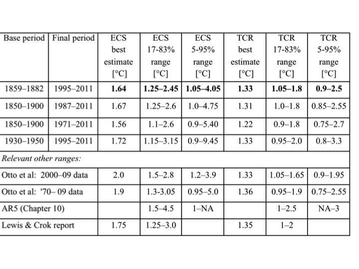
https://judithcurry.com/2014/09/24/lewis-and-curry-climate-sensitivity-uncertainty/
Table 1 gives the ECS and TCR estimates for the four base period – final period combinations used.
Full paper: https://niclewis.files.wordpress.com/2014/09/lewiscurry_ar5-energy-budget-climate-sensitivity_clim-dyn2014_accepted-reformatted-edited.pdf
So periods of stronger solar wind drive La Nina conditions, reducing atmospheric Water Vapour, and providing a strong negative feedback. Take it to the AMO scale, weaker solar wind since 1995 has driven a warm AMO, increasing water vapour in the lower to mid troposphere and reducing WV in the upper troposphere and lower stratosphere. Negative feedbacks all the way, less solar near infrared is absorbed at upper levels, and a greater WV greenhouse effect at mid-lower levels. The warm AMO even reduces CO2 uptake, another negative feedback.
sailboarder March 28, 2018 at 12:24 pm
Sounds good.. but the data sets he uses are not global. One might conclude for example that the 1910 to 1940 temperature rise is a warning to us that maybe nothing special is happening. Here is what Phil Jones had to admit:
1860 – 1880 0.16 C 20 years of warming, followed by 30 years of cooling.
1910 – 1940 0.15 C 30 years of warming, followed by 40 years of cooling.
1975 – 1998 0.16 C 20 years of warming followed by nearly 20 years of next to no warming(the so called “hiatus”).
Trends : Phil Jones CRU in East Anglia, UK. (Head of UK climate research unit, which tabulated the world wide temperature history. For confirmation, Google his 2009 interview by the BBC where he confirms these data trends in the temperature record)
That’s not what he ‘admitted’, here’s what he said in response to the question, (notice there’s no reference to the years of cooling you inserted):
“Temperature data for the period 1860-1880 are more uncertain, because of sparser coverage, than for later periods in the 20th Century. The 1860-1880 period is also only 21 years in length. As for the two periods 1910-40 and 1975-1998 the warming rates are not statistically significantly different (see numbers below).”
He was also asked:
“Do you agree that from 1995 to the present there has been no statistically-significant global warming”
To which he replied:
“Yes, but only just. I also calculated the trend for the period 1995 to 2009. This trend (0.12C per decade) is positive, but not significant at the 95% significance level. The positive trend is quite close to the significance level. Achieving statistical significance in scientific terms is much more likely for longer periods, and much less likely for shorter periods.”
Notice he didn’t say there was no warming as your post suggests, but that there was warming but there wasn’t enough data for it to be statistically significant at the 95% level.
In a follow-up interview the next year he pointed out that the extra year’s data allowed the trend to be statistically significant:
“Basically what’s changed is one more year [of data]. That period 1995-2009 was just 15 years – and because of the uncertainty in estimating trends over short periods, an extra year has made that trend significant at the 95% level which is the traditional threshold that statisticians have used for many years.”
“HadCRUT shows a warming 1995-2010 of 0.19C”
Assuming only atmospheric feedbacks account for Earth’s surface temperature overlooks the elephant in the room. What about the capacitors and diodes in the power supply? The largest ‘greenhouse effect’ that raises Earth’s average surface temperature is within the ocean rather than within the atmosphere. Oceans force surface heating during the night by convection, such that their surface barely cools.
The ocean is best understood as a heat sink, not a heat source (except to the extent that there is warming from below, particularly at the mid-ocean divergence boundaries).
The oceans as capacitor, yes that seems a reasonable comparison. They can store and release energy.
Also has a clear dampening effect, removes spikes, smooths the ‘current’.
Thermal reservoir:
“A thermal reservoir, a short-form of thermal energy reservoir, or thermal bath is a thermodynamic system with a heat capacity that is large enough that when it is in thermal contact with another system of interest or its environment, its temperature remains effectively constant.[1] It is an effectively infinite pool of thermal energy at a given, constant temperature. The temperature of the reservoir does not change when heat is added or extracted because of the infinite heat capacity. As it can act as a source and sink of heat, it is often also referred to as a heat reservoir or heat bath.
Lakes, oceans and rivers often serve as thermal reservoirs in geophysical processes, such as the weather. In atmospheric science, large air masses in the atmosphere often function as thermal reservoirs.”
https://en.wikipedia.org/wiki/Thermal_reservoir
Can act as a heat source, like at night when the upper ocean convects warmth to the surface.
Jaap wrote:
“Also has a clear dampening effect, removes spikes, smooths the ‘current’.”
Of the diurnal cycle, though big spikes are created by ENSO.
Christopher writes:
“(except to the extent that there is warming from below, particularly at the mid-ocean divergence boundaries)”
That is the ocean floor being the source and the ocean being the sink.
Magmatic intrusions warm the ocean, which passes some of the heat to the atmosphere. To this extent, the ocean is a source as far as the atmosphere is concerned.
The ocean surface is a source of heat every night regardless of the contribution by hydrothermal vent etc.
My question on all this is why didn’t the climate model peer reviewers do this or something similar years ago? I had to review complicated, iterative computer programs years ago in the nuclear industry and it was a requirement that an alternate means of verifying the computer results be performed to make sure the computer output made sense. You would usually do this by doing a simplified hand calculation, but sometmes it
took some creativity. That is exactly what Lord Monkton and friends did. If I was the judge I’d ask why did an outside group have to do it, and why didn’t the peer reviewers already do it? Maybe it was not a requirement here because it would be eventually validated with satellite monitoring (with billions spent in the interim) or maybe this is something engineers do (because lives are at stake) but scientists don’t, but whatever the reason it would have been good practice and most definitely financially prudent.
Dr. Roy Spencer peer reviewed “The Magic Temperature Feedback” by The Lord (Monckton) of the Rings”
http://www.drroyspencer.com/2018/03/climate-f-words/
http://i.myegy.to/images/679cdb58c95e.original.jpeg
The site that sells virtual calculaters
http://www.calqlata.com/
has a lot of science on it and one of their topics is on earth’s atmosphere. I quote from the site.
“Given that we know the density of air (ρₐᵢᵣ) at sea level is approximately 1292.8g/m³, the principal properties for each component gas at sea level are …
[units are evaluated to corroborate the formulas]:
The molecular density of air (ρᴹₐᵢᵣ) = ρₐᵢᵣ ÷ Σρᴹₓ.RAMₓ [g/m³ ÷ % x g/mole = mole/m³]
The molecular density of each gas (ρᴹₓ) = % . ρᴹₐᵢᵣ (mole/m³)
and the mass density of each gas (ρₓ) = ρᴹₓ . RAMₓ [mole/m³ x g/mole = g/m³]
Air pressure (pₐᵢᵣ) is 101325N/m²
Gas pressure (pₓ) = % . pₐᵢᵣ (N/m²)
Gas mass pressure (pmassₓ) = pₓ . (r+H)² ÷ G . m₁ [N/m² x m² ÷ N.m²/kg² x kg = kg/m²]
which is the mass of gas in the atmospheric column and ‘H’ is the altitude of its centre of mass
i.e. 50% of the mass lies above this altitude and 50% of the mass lies below it
To conclude for the principal gases in the earth’s atmosphere @ 273.15K:
gas RAM percentage mole density mass density mass pressure
g/mole ≈% (ρᴹₓ) mole/m³ (ρₓ) g/m³ (pmassₓ) g/m²
N₂ 28.0134 78.087% 34.42594855 964.387867 8087362.21571
O₂ 31.9988 20.95% 9.236154828 295.5458711 2169233.80954
Ar 39.948 0.93% 0.410005918 16.37891643 96258.45023
CO₂ 44.095 0.03% 0.013225997 0.583200354 3104.60026
Ne 20.1797 0.0018% 0.00079356 0.0160138 186.42350
He 4.002602 0.00052% 0.000229251 0.000917599 53.85568
CHₓ 16.04246 0.0002% 8.81733E-05 0.001414517 20.71372
H 1.00794 0.000048% 2.11616E-05 2.13296E-05 4.97129
N₂O 44.0128 0.00005% 2.20433E-05 0.000970189 5.17433
O₃ 47.9982 0.000004% 1.76347E-06 8.46432E-05 0.41391
H₂O 18.01528 2% 0.881733158 15.88466972 207137.22427
Air # 29.324 101.99962% 1292.8 10563407.45
# 99.99962% air including 2% water
0.00038% trace elements are ignored
mole density of air = ρₐᵢᵣ ÷ RAMₐᵢᵣ = 1292.8 ÷ 29.324 = 44.08666 moles/m³
Incorporating the ideal gas law; p.V = n.Rᵢ.Ṯ
where:
p = pressure = force ÷ area (F/A)
V = volume
n = number of moles of substance
Rᵢ = ideal gas constant (8.3143 J/K/mole)
Ṯ = temperature (absolute)
into the equation (F = G . m₁ . m₂ / (r+H)²) we can calculate altitude ‘H’ as follows:
Gravitational acceleration variation with altitude
Fig 2. Atmospheric Temperature Profile
F/A . V = n . Rᵢ . T
F = n . Rᵢ . T . A / V
F = n . Rᵢ . T / H (H = V/A)
If m₂ = n.RAM/1000 kg, then …
F = G . m₁ . n.RAM/1000 / (r+H)²
n . Rᵢ . T / H = G . m₁ . n . RAM / 1000 / (r+H)²
Rᵢ . T / H = G . m₁ . RAM / 1000 / ( r² + 2rH + H²)
(r² + 2rH + H²) = H . G . m₁ . RAM / Rᵢ / T / 1000
H² + H.(2r – G . m₁ . RAM / Rᵢ / T / 1000) + r² = 0
a = 1
b = 2r – G . m₁ . RAM / Rᵢ / T / 1000
c = r²
H = {-b-√(b² – 4.a.c)} / 2a
By entering the correct altitude temperature for the latitude and additionally modifying for the effects of centrifugal force (v²/r) you will find the correct value for ‘H’ for each atmospheric gas.
Repeat this procedure for the uppermost 50%, modifying m₁ and r to include the gas below ‘H’, and you will find H for the upper 50% in the gas column. Keep going (for the uppermost 25%, 12.5%, 6.25%, etc.) and you will discover how the mass pressure of gas varies with altitude.
The earth’s atmospheric gases
Fig 3. Earth’s Atmospheric Gases @ Altitude
Conclusion
From the above formula CalQlata has demonstrated that …
‘For any atmospheric gas with the same RAM at a given temperature, the altitude of a specified percentage of its total mass will always be identical ‘
Therefore irrespective of the total mass of a particular gas in the atmosphere, for any given temperature; its “percentage mass vs altitude” profile will not change.
Whilst weather patterns in the Troposphere will alter these theoretical pressures and densities locally, such variations will not alter the overall picture.
Using the same calculation procedure, we also generated ‘mass pressure-altitude’ plots for each gas (Fig 4), providing the mass of gas above the altitude in question.
Atmospheric Gas Ceilings
The following are CalQlata’s practical and theoretical ceilings⁽⁴⁾ for each gas in the earth’s atmosphere at the equator and the poles:
practical ceiling (km) theoretical ceiling (km)
Gas equator poles equator poles
N₂ 3998.95038 3458.49594 8103.50773 7031.05161
O₂ 3118.26617 2665.80287 6204.52442 5386.80279
Ar 1985.51194 1647.63729 4008.86933 3462.06235
CO₂ 1525.38322 1236.35231 3215.26978 2753.62086
O₃ 991.62283 776.08888 2378.94412 2001.80321
CF₂Cl₂ 159.34693 107.41656 459.18917 327.51499
The top of the Exosphere is generally accepted as the upper limit of the earth’s atmosphere and for all practical purposes this may well be the case as it is difficult to consider ‘a few molecules per cubic meter’ constituting a viable atmosphere, but for the purposes of theoretical calculations even such low densities as these should not be ignored.
Therefore, CalQlata set out to define the actual quanties of each gas in the earth’s atmosphere, and according to our calculations, there remains 14624.816171kg of nitrogen, 30.753837772kg of oxygen and traces of Argon and other gases (hydrogen helium, etc.) above the top of the Exosphere.
Comparing the earth’s gravitational attraction on each atmospheric gas molecule with its centrifugal force at its theoretical ceiling today (see Atmospheric Gas Ceilings above), we can deduce the following:
molecule RAM m H R Fᵍ (+ve) v Fᶜ (-ve) F
(kg) (km) (m) (N) (m/s) (N) (N)
N₂ 28.0134 4.69E-26 8103.51 1.448E+7 8.885E-26 1053.137 -3.589E-27 8.526E-26
O₂ 31.9988 5.35E-26 6204.52 1.258E+7 1.3443E-25 915.039 -3.562E-27 1.309E-25
Ar 39.948 6.68E-26 4008.87 1.039E+7 2.463E-25 755.366 -3.67E-27 2.426E-25
CO₂ 44.01 7.36E-26 3215.27 9.593E+6 3.181E-25 697.654 -3.7347E-27 3.143E-25
O₃ 47.9982 8.03E-26 2378.94 8.757E+6 4.1630E-25 636.835 -3.718E-27 4.126E-25
CF₂Cl₂ 120.914 2.02E-25 459.19 6.837E+6 1.72E-24 497.226 -7.313E-27 1.713E-24
proton 1 1.67E-27 8103.5 1.448E+7 3.1715E-27 1053.137 -1.281E-28 3.043E-27
where: m = mass; H = maximum ceiling height; R = distance between centres of mass; Fᵍ = gravitational force on molecule @ H; v = maximum velocity of molecule @ H; Fᶜ = centrifugal force on molecule @ H; F = resultant force on molecule @ H {+ve = towards earth & -ve = away from earth}
Gravitational force is lowest and centrifugal force is greatest in a gas at its ceiling. So if the resultant force (F) for all gases are positive (in the above table) at their atmospheric ceilings it means that no molecule can escape the earth’s gravitational attraction as a result of centrifugal force. This point is reinforced by the hypothetical case for a proton at the ceiling for nitrogen.
Given that the earth’s atmosphere is unlikely ever to have contained sufficient quantity of any gas to have achieved a ceiling at the earth’s escape altitude (35,840km)⁽⁹⁾, the above table confirms that no part or type of any atmospheric gas has ever been thrown into outer-space as a result of centrifugal force.
“Greenhouse” Effect
The “Greenhouse” effect is a reference to the ability of atmospheric gases to retain heat and thereby raise a planet’s surface temperature, which would otherwise fall to that of outer-space (≈2.73K). The ability of any gas to retain heat energy is defined by its ‘Specific Heat Capacity’.
Specific heat capacity (cp) is measured in J/kg/K (btu/lb/R) and describes how much energy a unit mass of the substance will require for each degree (K or R) of change in temperature.
If we know the mass of each gas in the earth’s atmosphere, we can calculate the amount of heat energy stored in that gas and therefore its contribution to the “Greenhouse” effect.
The mass of each gas in the earth’s atmosphere was established from their pressures in the above Calculation Procedure; and by multiplying the specific heat capacity by its mass we can determine the heat energy stored in each gas.
Whilst our calculation is valid for a particular temperature (273K), and the specific heat capacity of most gases rises with temperature, the relative contribution from each gas in the earth’s atmosphere will remain largely unchanged.
The following table lists the results from these calculations:
Gas cp Mass Stored Energy %age of Air
J/kg/K kg J/K
N₂ 983 4.13091006E+18 4.060684588E+21 79.5209485%
O₂ 919 1.10774396E+18 1.018016698E+21 19.9359619%
Ar 531 4.91366416E+16 2.609155669E+19 0.5109546%
CO₂ 844 1.58453127E+15 1.337344390E+18 0.0261894%
Ne 1030 9.50566787E+13 9.790837905E+16 0.0019174%
He 5240 2.74608183E+13 1.438946878E+17 0.0028179%
CHₓ 2200 1.05618532E+13 2.323607701E+16 0.0004550%
H 14300 2.53484477E+12 3.624828014E+16 0.0007099%
N₂O 880 2.63837434E+12 2.321769416E+15 0.0000455%
(H₂O) (1859) (1.05618532E+17) (1.963448508E+20)
Totals 5.28951345E+18 + H₂O 5.106433796E+21 + H₂O 100% + H₂O
The stored energy values in the above table assume that all the atmospheric gases are at 273K, which is not correct. Temperature drops and rises with altitude (see Fig 2) and the specific heat capacity of all gases rise and fall with temperature, not necessarily at the same rate but very similarly, except where certain gases fade out at various altitudes, the total percentage contribution of stored heat is virtually identical no matter how you perform this calculation.
The temperature of the earth’s atmosphere is directly proportional to the heat energy retained in its gases. Therefore, a change in the mass of any gas in the earth’s atmosphere will have a consequential effect on the earth’s surface temperature.
The sum of all the ‘Stored Energy’ values in the above table (5.106E+21J/K) represents the energy in the atmosphere that would be required to raise the temperature of all the gas molecules to 273.15K.
Therefore, every single degree (1K) of this temperature must be generated by 1.8695E+19J of heat energy. In other words, to raise the temperature of the atmosphere by 1K (to 274.15K) you would need to increase the total Stored Energy by 1.8695E+19J. ##########################################################################################################################################################################################################################################################################################################
The above value is the most important point in this whole thesis. It will be referred to in Alan Tomalty’s additional argument at the end.
To conclude;
because nitrogen is responsible for 79.52% of the atmosphere’s stored energy, a 1% change in its mass will significantly affect surface temperature
On the other hand;
a significant increase (e.g. >1000%) in the mass of gases such as neon, carbon dioxide, helium, hydrogen that together constitute less than 0.039% of the atmosphere’s stored energy will have very little effect on the earth’s surface temperature.
However, if we apply the laws of thermodynamics to the above argument these effects are not quite so straight forward, for example; …
CO₂
Along with other carbon gases, CO₂ is today charged with being the principal cause of Global Warming (see Global Warming below) because it is a “Greenhouse” gas. This claim is made because of its low specific heat capacity; i.e. it requires less energy input to raise its temperature by 1K than the more abundant atmospheric gases (except argon). However, its contribution to the earth’s atmospheric temperature can only be considered in conjunction with its relative mass.
Applying the specific heat equations to each gas in the earth’s atmosphere reveals the following retationship between CO₂ and its effect on earth’s atmospheric temperature:
Gas cp CO₂ CO₂ x 0.9 # CO₂ x 10
J/kg/K kg kg kg
N₂ 983 4.1309E+18 4.1309E+18 4.1309E+18
O₂ 919 1.1077E+18 1.1077E+18 1.1077E+18
Ar 531 4.9137E+16 4.9137E+16 4.9137E+16
CO₂ 844 1.5845E+15 1.4261E+15 1.5845E+16
Ne 1030 9.5057E+13 9.5057E+13 9.5057E+13
He 5240 2.7461E+13 2.7461E+13 2.7461E+13
CHₓ 2200 1.0562E+13 1.0562E+13 1.0562E+13
H 14300 2.5348E+12 2.5348E+12 2.5348E+12
N₂O 880 2.6384E+12 2.6384E+12 2.6384E+12
Air: mass: 5.2895E+18 kg 5.2894E+18 kg 5.3038E+18 kg
cp: 965.3882 J/kg/K 965.3918 J/kg/K 965.0618 J/kg/K
Ṯ: 293.7471 K 293.7548 K 293.0563 K
The energy supply in the above calculations is the same for each column: 1.5E+24J
As this is a constant in each calculation changing the energy input will not alter the relative results
Conservatively based upon the assumption that mankind generates 50% of the earth’s CO₂: 0.9 = 90% = 50% + 50% x 80%
As can be seen in the above table, increasing the quantity of CO₂ actually decreases the temperature of the earth’s atmosphere.
This phenomenon is due to the fact that the additional mass of the increased CO₂ in the atmosphere (CO₂: 1.585E+15 kg 965.0618 J/kg/K).
As a result, it can be concluded that significant increases in atmospheric CO₂ will have no appreciable effect on the temperature of the air, other than to reduce it slightly.
In fact increasing any gas in a mixture that contains a fixed amount of heat energy will cause the temperature of the mixture to drop as the energy is distributed over a greater number of molecules.
For example, if 1kg of the earth’s atmospheric mass holds 235156.5J of energy and has a temperature of 273K; increasing its mass by 1% with:
N₂ reduces the temperature of the gas mixture to 269.4K
O₂ reduces the temperature of the gas mixture to 270.6K
Ar reduces the temperature of the gas mixture to 272.0K
CO₂ reduces the temperature of the gas mixture to 270.9K
Therefore, simply increasing the earth’s atmospheric CO₂ cannot increase its temperature.
However, if the entrained heat energy in the gas mixture is also increased by 2% (for each of the increases shown above):
N₂ increases the temperature of the gas mixture to 274.785K
O₂ increases the temperature of the gas mixture to 276.01K
Ar increases the temperature of the gas mixture to 277.4K
CO₂ increases the temperature of the gas mixture to 276.35K
clearly showing that Argon has a greater effect on atmospheric temperature than CO₂
The above increase in entrained heat (2%) along with the gas mass increase (1%) represents the following percentage increases for each gas in the mixture:
N₂ would need to increase by 1.28%
O₂ would need to increase by 5%
Ar would need to increase by 200%
CO₂ would need to increase by 2564.1%
proving that …
only a small percentage increase in N₂ and O₂ is needed to raise the temperature of the earth’s atmosphere by ≈3K
almost double the amount of Ar is needed to achieve a similar rise in temperature
but more than 26 times current levels of CO₂ are required to generate a similar rise in temperature.”
*************************************************************************************************************
From here on is my original analysis that extends calqlata’s computatations.
Further to the above in quotations, all of which you will find on calqlata’s site are my thoughts.
Dont forget that even though all the above calculations were for a starting temperature at 273K, the linear proportionality of heated gases dictates that the calculations are good for any temperatures that you would encounter in the troposhere.
If you double the CO2 and assume that every CO2 molecule is then maxed out with its maximum IR that it can absorb an additional
1.337344390E+18 of heat that is now trapped in the atmosphere by the additional CO2. However as in the above where it is ###########
To raise the temperature of the atmosphere by 1K no matter what temperature you are at you would need an additional 1.8695E+19 Joules/kg
The above analysis assumed that the atmosphere was warmed from 273K to 288K( average earth temperature) because of greenhouse gases. The generally accepted view is that without greenhouse gases susch as H2O and CO2, the earth would be 255K or -18K below freezing. Therefore the above analysis of the amount of energy needed to maintain the earth equilibrium temperature at 288K has to be multiplied by a factor of 2.2 ((18+15)/15 ).
Taking the ratio of the above 2 numbers and deleting the extra significant digits in the numerator so as to match the 4 significant digits in the denominator you end up with an initial specific heat ratio for CO2 doubling of ~ 0.07. However you have to apply the 2.2 factor above so that you end up with 0.154 as the final specific heat ratio for CO2 doubling. This means that a doubling of CO2 only raises the temperature 0.154K
YOU WOULD NEED 6.5 TIMES AS MUCH CO2 TO RAISE THE TEMPERATURE 1K. Now the CAGW scientists will argue that the water vapour forcing by the increase in CO2 starts at any increase in temperature no matter how small. Well we know that temperatures are local and the variability is dwarfed by the evaporation and precipitation and accompagnied temperature decreases and increases. However even if we accept the preposterous assumption that water vapour forcing commences at any small temperature increase, the CAGW scientists have to prove that there has been an increase in the average water vapour(H2O) content of the atmosphere in the past 60 years or so. The Goddard Space Institute a division of NASA had a project team that was measuring the H2O content of the atmosphere from 1989 to 2009. They could not show or prove that the H2O content was any different in the 20 years of measuring so the then director of the Goddard Space Institute Dr. James Hansen shut the project down. Until NASA or anyone else proves that there is more H2O in the atmosphere today than there was in 1950 ( or if there is a definite upward trend in any given time period of not less than 10 years) we have to assume that the Global warming theory of AGW caused by CO2 is simply one big hoax.
Alan,
Sounds like you support the mass based hypothesis. Would that be right?
I believe that the above argument is a complete bust to the CAGW theory.
“The most significant objection to our argument came from Roy Spencer, who said official climatology defines a temperature feedback as an extra forcing induced by a change in temperature, but not by the original temperature itself.
That is indeed the definition. But merely because official climatology says white is black, we should not be too hasty in bidding farewell to white.”
~ MoB ~
Bizarre fantasy world … an attempt to obfuscate and buffalo a judge. It’s not like making misleading presentations to non-technical audiences. There will be scientists who understand, can explain the foolery, and can point and laugh as you’re escorted from the room.
And is the furtively pseudonymous “John@EF” capable of producing any scientific argument, rather than a characteristically malicious and characteristically false allegation?
Monckton of Brenchley said March 28, 2018 at 8:49 pm
“Don’t whine. Wait for the paper.”
Mr. Monckton is the undisputed leading expert on the politics of global warming. Further his knowledge of many things; including Latin, British peerage, and indeed, the general drift of scientific papers on climate change exceeds my own. However, he does NOT know more about electronics, feedback theory, or signal processing than I do. In fact, one may, with demonstrable fairness, assess that he knows very little about such things (below).
We often quite reasonably judge a person’s technical acumen by his/her apparent ability to grasp even the simplest matters with which we ourselves are very familiar. To the extent that the person is not upfront about his/her limitations, (instead extolling consultation with unnamed experts), our doubts are understandably increased.
Few of us would object to having someone with superior knowledge pointing out our errors. We would likely thank the person teaching us, and all have a good laugh. No offense would be intended, nor taken.
In Sept of 2016, Monckton stated in his “feet of clay” postings here on WUWT that positive feedback could not be more positive than +0.1. {Red flag 1} Many here knew he was WRONG. And many here of course did NOT know (perhaps – any more than he did) that he WAS wrong; and these masses resented his error being even suggested, regarding it as just a mechanical attack on skeptics of CAGW. We skeptics need to be vigilant, first of all, of our own mistakes.
I would NOT keep harping on his error were he to simply have stated (or to now state) that he was wrong, and perhaps even apologize. Instead he persisted with invective (another of his undisputed talents!) against the engineers here, quoting one of his experts who had THREE PhDs; then messing up his arguments with failures to properly count the multiple-negatives within phrasing – and with the most egregious put-offs of “Don’t Whine – Wait”. We waited a year and a half for Parts 4 and 5 of “feet”, sincerely hoping the delay was not an issue of health. Nothing. Recently, an abandonment of “feet” blamed on (our?) harassment.
In the recent “amicus” revivals, which I freely admit may or may not be correct, Monckton has demonstrated yet again a lack of knowledge of the simplest of things, and refused to provide needed diagrams/circuits. We get – again “Don’t whine. Wait for the paper.”
In the latest, he has claimed a feedback without an amplifier is not seen in all the (electronics) literature. I pointed out that there IS generally an amplifier SHOWN, denoted A (or something) and that A can be 1 (unity, or any other number) and often is. {Red flag 2} He replied that my view is not exactly the same thing. Of course it is EXACTLY the same thing – a general “variable” assigned a specific numerical value. Again, Monckton lacks the technical fluency that would suggest he has the right to be offering information as though he were an expert, or even capable of making a particular point in question.
For some reason, in the “amicus” thread, Monckton offered up (ad hoc), a diagram with the top link: Figure 3.1 of Bode (1945) – perhaps in response to my “hectoring” about a needed flow-graph. Unfortunately, the figure is incomplete/misleading. {Red flag 3.} It lacks directional arrows on the flow paths. [Amusingly, many library editions have been “corrected” by readers.] The path through the Beta box should be right-to-left (that is, feedback), but it doesn’t show; nor are directions of signals in/out of the two nodes shown. No one uses this book today – if for no other reason than it uses vacuum tube (valve) examples.
Frankly, I think some here (me included) treat Mockton with less than 100% deference not out of disrespect but in return for the fact that he enters someone’s domain in error and has not the courtesy to fully apologize and leave quietly.
Well said. Your comment puts me in mind of what Michael Crichton called the “Murray Gell-Mann amnesia effect.”
Thanks Joe. True for many of us. When I got involved fighting the local municipality against eminent domain, I was familiar with the local reporting of the conflict and was even the source (even to some actual wording submitted) of some. The reporters still usually managed to change things – wrong. I was for a few days wondering at the “coincidence” that the stories I knew about happened to be the ones they got wrong. Then I figured it out. Larger lesson there.
For credibility, I suspect you need to get the simple things right first. Somebody knows. At least a few who don’t mind speaking up, we hope.
Readers should know that the contemptible Mr Born, having been caught out in a malicious misrepresentation here long ago, has never lived it down and has blubbed childishly at every opportunity since. His comments, which seldom offer anything recognizable as science, may be discounted as mere spite. Having lied before, he has shown that he has not the slightest interest in the objective truth.
As for Mr Hutchins, he too is guilty of misrepresentation. He has artfully rewritten what I wrote about the likely region of stability in a chaotic object on which multiple feedback processes bear. He has stated, falsely and knowingly, that I had written that “positive feedback could not be greater than +0.1”. I had not written anything of the kind. Indeed, I had shown a graph in which the feedback fraction exceeded +1.0. I had, however, pointed out, reasonably enough, that in the design of electronic circuits intended to operate stably in variable operating conditions and with potentially substandard componentry it is often the custom to design in a maximum feedback fraction of 0.1, or even 0.01 where possible.
Mr Hutchins’ second false statement is to the effect that I had “claimed a feedback without an amplifier is not seen in all the (electronics) literature”. What I had in fact said was that a commenter (actually Mr Stokes) had said he had never seen such a circuit, and that I had not seen one either. However, as explained in this series, we had built not one but two such circuits, precisely so that we could set the amplifier gain factor to unity, in effect rendering our circuit one in which the input signal was not amplified directly and yet was modified by any nonzero feedback fraction.
Mr Hutchins’ third false statement is that I had supplied an “incomplete” or “misleading” graph. I had in fact simply reproduced, without any alteration whatsoever but with correct attribution, Fig. 3(1) of Bode (1945). Mr Hutchins, whose ignorance is as bottomless as his arrogance, seems unaware that in that era it was commonplace to display feedback loops without cluttering them with arrows. The triangle of the gain block points in the direction of travel, and (though Mr Hutchins is very careful to conceal this fact from the readers of his hate speech) Bode expressly defines the beta feedback fraction as the “return transmission characteristic” and explains that the the current is returned from the output node via the feedback block labeled beta to the input node. The general reader, considerably more intelligent than the ape-like Hutchins, is thus able to discern without pretty little children’s arrows what is the direction of the current.
The three “red flags” of which Mr Hutchins speaks are thus red flags indicating his dishonesty. One understands that he and others here are mortified to discover that the Party Line to which they have devoted enormous effort is in a fundamental respect erroneous. But they will not improve matters by blatant fabrication. Matters are now out of their hands, and all their hate speech will make no difference to the outcome.
As to the obsession of both Mr Hutchins and the dreadful “Phil.” with qualifications – how can Monckton dare to question the Party Line when in their opinion he has no certificate of appropriate Socialist training in any relevant subject? – five of my co-authors are PhDs, and three of these are Professors. They have the relevant certificates. It is no use, therefore, whining about my apparent lack of qualifications. We know that, these days, academe is overwhelmingly totalitarian and that, therefore, mere rational argument and formal demonstration count for nothing compared with certificates of Socialist training. So we have provided both.
Bernie Hutchins March 29, 2018 at 2:15 pm
Monckton of Brenchley said March 28, 2018 at 8:49 pm
“Don’t whine. Wait for the paper.”
Mr. Monckton is the undisputed leading expert on the politics of global warming. Further his knowledge of many things; including Latin, British peerage, and indeed, the general drift of scientific papers on climate change exceeds my own. However, he does NOT know more about electronics, feedback theory, or signal processing than I do. In fact, one may, with demonstrable fairness, assess that he knows very little about such things (below).
We often quite reasonably judge a person’s technical acumen by his/her apparent ability to grasp even the simplest matters with which we ourselves are very familiar. To the extent that the person is not upfront about his/her limitations, (instead extolling consultation with unnamed experts), our doubts are understandably increased.
Yeah, although it is not an area of research of mine I did use analog computers to model thermokinetic systems years before Monckton was a cub reporter on The Yorkshire Post. I have since used Op-amps in a lab class to teach the students how feedback can generate oscillations and I find some of the misinformation on the subject here disturbing. Regarding the positive feedback, for the students to get their circuits to oscillate it was necessary to have a gain of greater than unity, the most common reason for the failure to oscillate was that the students had chosen the wrong resistance so that the gain was slightly less than 1 (~0.99) and therefore stable!
Quite right Phil. And it was essentially impossible to hold the gain at exactly 1. You had to set the gain a tiny tad high and let the oscillation bump its head – like with a regulating Zener diode.
Or, some oscillators had a tiny “grain of wheat” light bulb inside! A trouble light for repairs?!? Nope, the topic here is feedback. The oscillation drove the light bulb, and if the amplitude wondered up a bit, the bulb got brighter and its resistance increased, cutting back the gain. Thermal feedback. Essentially instantaneous. To clever for words. Hope the engineer got rich.
Yes Bernie, exactly. We used the Wien bridge circuit, as you say it needs to ‘bump its head’ so the sine wave is slightly flattened at the max. I looked at the variant with the incandescent bulb it really is very clever.
Phil – the case of a digital sinewave oscillator is even more diabolic. You would seem to need to set the poles exactly on the unit circle in the z-plane. Thus real^2+imag^2 = 1. Quite impossible with finite wordlength. But, to the surprise of most, the sequence (automatically) falls into some convenient tiny superimposed limit cycle that is usually good enough, or better – stable forever with a tiny shift away from the design frequency.
I googled “digital sinewave oscillator” to make sure I understood what is being talked about. And, sure enough, it took me to Electronotes 348, which explains a lot.
If we are right it’s game over
BUT
Even if we are wrong (e.g. it’s gravity after all, etc, etc)
It’s STILL game over.
Because the new feedback equation is the CORRECT formulae for the CAGW argument. So they would either have to accept it OR come up with an entirely new thoery of CAGW which negates the obvious feedback “error”.
Meanwhile certain scientists quietly work on the other theories which may or may not be right. And it’s the latter that are exciting because eventually we ARE going to find out how the atmosphere REALLY works.
I will be interested if this goes to a trial. In federal court the expert for both sides will need to provide a written report on their findings and opinions. In Federal court all opinion based on science must follow the scientific method. All experts are subject to a Daubert challenge (see Daubert v Merrill Dow Pharmaceuticals) from the opposing party. To survive a Daubert challenge the expert must prove his methodology to form his opinion was correct. This doesn’t mean his opinion is valid, but he must prove a valid methodology to form his opinion. I do not see any climate change promoting expert being able to prove their methodology is correct. The scientific method requires an experts methodology must be able to be tested. Computer Modeling is fine, but if the computer modeling is faulty it won’t be accepted. So far the only extreme global warming temperatures studies I have read about have been generated by computer models and not by actual data.