This paper deals with the central argument that skeptics bring up about claims of global warming: How do you separate the temperature signal from the base components like natural variation, human land-use influence, micro-site bias, measurement errors and biases, and other factors to get the “true” global warming signal?
The answer is that you can’t, at least not easily.
With the surface temperature record, it’s somewhat easier since you can observe some of those elements directly and separate them (such as we’ve done in our surfacestations project for land-use microsite biases), but in the ocean, everything is homogenized by the ocean itself. All you can look for is patterns, and try to disentangle based on pattern recognition. That’s what they are trying to do here.
Disentangling Global Warming, Multidecadal Variability, and El Niño in Pacific Temperatures
Authors
Robert C. Wills, Tapio Schneider, John M. Wallace, David S. Battisti, Dennis L. Hartmann
Abstract
A key challenge in climate science is to separate observed temperature changes into components due to internal variability and responses to external forcing. Extended integrations of forced and unforced climate models are often used for this purpose. Here we demonstrate a novel method to separate modes of internal variability from global warming based on differences in time scale and spatial pattern, without relying on climate models. We identify uncorrelated components of Pacific sea surface temperature variability due to global warming, the Pacific Decadal Oscillation (PDO), and the El Niño–Southern Oscillation (ENSO). Our results give statistical representations of PDO and ENSO that are consistent with their being separate processes, operating on different time scales, but are otherwise consistent with canonical definitions. We isolate the multidecadal variability of the PDO and find that it is confined to midlatitudes; tropical sea surface temperatures and their teleconnections mix in higher-frequency variability. This implies that midlatitude PDO anomalies are more persistent than previously thought.
http://onlinelibrary.wiley.com/wol1/doi/10.1002/2017GL076327/full
Unfortunately, the article is paywalled, even though it is publicly funded by the National Science Foundation. Grant Number: AGS-1549579. The author’s webpage at UW doesn’t have a draft copy, so I can’t comment further. If anyone has access they can provide me, I’ll be happy to update the article.
It is unfortunate (and wrong) that publicly funded science gets put under lock and key from the public examination of it.
Anthony–Here is a link to the paper.
https://www.dropbox.com/s/fe7z2ffnlt7tsnv/Wills_et_al-2018-Geophysical_Research_Letters.pdf?dl=0
Or the .pdf file, free, here: https://www.atmos.washington.edu/~david/Wills_etal_PNAS_submitted_2017.pdf
Thanks!
Google search for the title and there are draft copies available, but you probably need permission to to post a draft copy.
So where do they assign the omission error of leaving out the AMO and the multi-decade variability of the AMO?
These guys live on the West Coast and probably don’t know that the Atlantic exists.
Oh, okay
They might not be able to spell AMO!
The wisdom of Solomon.
That explains a lot.
I reckon there is another mob on the east coast who are not aware of the Pacific which would explain the other missing link to relity.
This is my KISS* study:
http://www.woodfortrees.org/plot/hadcrut3vgl/mean:121/mean:37/from:1870/to:2010/plot/esrl-amo/mean:121/mean:37/plot/hadcrut3vgl/from:1870/to:2010/trend
Starting on top of an AMO wave 1870 to another one 2010 you have ruled out the AMO influence.
You get 0.75°C total temperature rise or 0.5°C per century.
Using 1910 (Bottom of AMO) to 2010 (Top of AMO) you get 0.7 °C per century
*Keep it small, simple.
Johannes Herbst
Your chart displays a land/ocean surface temperature chart, HadCRUT3, which was discontinued in 2014, replaced by HadCRUT4. Why would you compare an obsolete land/ocean temperature data set against AMO when Hadley supplies an ocean-only data set that is up to date, HadSST3? It’s right there at WfTs.
Also, you’ve only added the linear trend for the temperature data set. Add the linear trend to the AMO data and you’ll see that, over the period you have selected, it is actually ‘downwards’. So we have a flat or downwards trend in AMO and a long term warming trend in ocean temperatures. If there’s any long term correlation between AMO and SSTs then it’s a slightly negative one!
From your link with amendments as detailed above, the chart below shows AMO versus SST (HadSST3) with trend lines for both.
KISS, control for the Urban Heat Island Effect and only use Temperatures over the ocean. The Oceans control 2,000x the heat of the atmosphere, so they clearly control the atmospheric temperatures. Therefore, to explain the atmospheric temperatures, you have to explain the ocean temperatures.
Understand the Oceans, Understand the Global Temperatures
Here at CO2isLife we have consistently maintained that to understand the climate you have to understand the oceans. The oceans, not CO2, is are the major drivers of global climate and temperatures. The oceans contain 2,000x more energy than the atmosphere, and CO2’s only defined mechanism by which to affect climate change is by thermalizing … Continue reading
https://co2islife.wordpress.com/2018/02/22/understand-the-oceans-understand-the-global-temperatures/
Isolating the Contribution of CO2 on Atmospheric Temperature
In any serious scientific experiment, efforts are made to “control” for as many exogenous factors as possible. The whole purpose is to isolate the impact of the independent variable on the dependent variable. ΔWeightloss = ΔCaloric Intake + ΔExercise + ΔBase Metabolism + error. To minimize the error of the model (maximize explanatory power), variables outside … Continue reading
https://co2islife.wordpress.com/2018/02/14/isolating-the-contribution-of-co2-on-atmospheric-co2/
Completely agree! Publicly funded should be publicly available. We don’t need to pay for it twice! (Or even once if it’s abused poor politico-science; not saying it is, but if I can’t read it to determine value, I can’t determine its worth)
Agree in principle, but the journal needs some income.
Why does the public need the journals?
From the paper…
“The first LFP shows a nearly uniform warming pattern, corresponding to a 0.67∘C per century warming of Pacific SSTs throughout the record (Figure 1a) [1900-2016]. The warming of tropical Pacific SSTs is notably uniform, withouta clear El-Niño-like or La-Niña-like warming trend. There is detailed temporal structure to the global tempera-ture rise, with periods of reduced global warming between the mid-1940s and late 1980s and between 1998 and 2013.”
Doesn’t that correspond roughly to what we suspect already and which is not well correlated to the CO2 pattern?
They have good “data” going back to 1900?
The 1940’s-1980’s are years of “reduced global warming”? I thought global temps dropped a degree, which would equal all century warming. There was, after all, a consensus that an ice age was imminent.
Waste of time. If ENSO was internal variability, El Nino wouldn’t increase in frequency and intensity during solar minima, nor would negative AO/NAO.
It’s not quite so clear cut. Internal variation always has a cause, an excitation that sets it in motion. It can be sensitive to ongoing excitation, but a part of the response can be dependent on excitations long past, effectively independent of what is happening in the present.
For example, consider your coffee cup. You can swirl it around, and the coffee starts sloshing about. But, if you stop swirling it, the coffee doesn’t just immediately come to rest. It keeps sloshing around a bit, due to your past swirling motion up to that time.
When you’ve got a coffee cup as big as the oceans, you’ve got a long train of stored excitation extending far into the past.
Bartemis, good analogy especially with the added timeline. Ocean “sloshing” seems to go on for decades, if not centuries. I have searched for the latest estimate of the age of “bottom water” recently but if my memory serves me it is long. I was taught it was like plucking a really long guitar string.
In exactly the same way our CO2 is going to be sloshing around the atmosphere causing future excitation for hundreds of years. From IPCC AR5 WG1.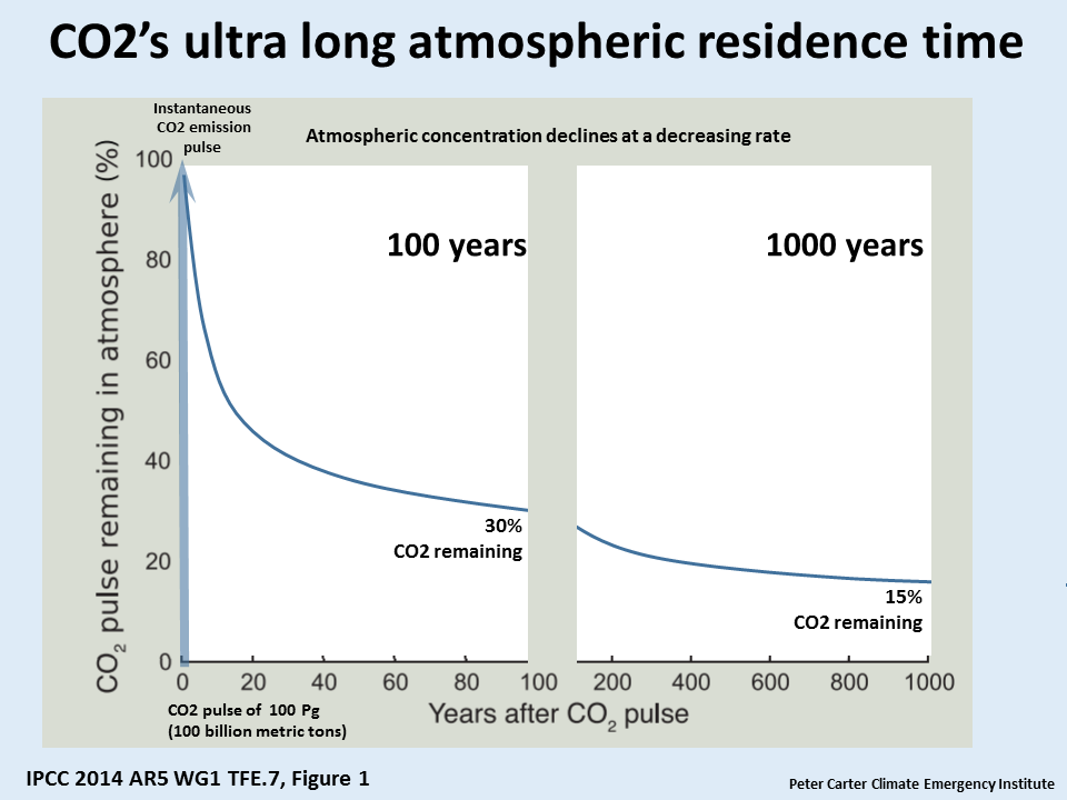
CO2 doesn’t slosh, and the evidence indicates that CO2 provides precious little “excitation”.
@Zazove:
Maximum atmospheric residence time of CO2 according to 37 different studies:
http://c3headlines.typepad.com/.a/6a010536b58035970c0120a5e507c9970c-pi
All but 6 show less than 10 years.
Rational Db8: You are confusing the time that an individual CO2 molecule is in the atmosphere, with the time that an increase in the total atmospheric concentration of CO2 lasts. Individual CO2 molecules can go in and out of the atmosphere without affecting the total concentration, as long as (on average) one molecule goes in for every one molecule that goes out. https://skepticalscience.com/co2-residence-time.htm
As Bartemis says: “sensitive”, lets keep our fingers crossed “precious little” isn’t too much.
We don’t have to keep our fingers crossed.
CO2 levels on this planet exceeded 5000ppm in the past, and nothing bad happened.
Going from 280ppm to 500-600ppm even less will happen.
Of course the 2 time scales are connected only by the total numbers remaining. The real factors are the rate at which CO2 dissipates (ie self destructs) in the atmosphere, the rate at which CO2 escapes from the atmosphere into the oceans and the rate at which CO2 enters the atmosphere because of mankind and the rate at which CO2 enters the atmosphere from the oceans..Only by knowing all 4 rates can you accurately determine what the future level will be. In the past 38 years, mankind has put 75% more fossil fuel emissions into the atmosphere but the actual CO2 levels have gone up only 21% in those 38 years. Has anybody determined how CO2 gets pulled into the oceans?. Has anybody determined any of those 4 rates? Has anybody determined how exactly does CO2 enter the atmosphere from the oceans? Has anybody got a hold of the famous radiation transfer equations that warmists like to talk about and I am not referring to the simple (x no of watts forcing = y no. of degrees warmer). Can anybody say for certain(99% centile) that the planet has warmed 0.7C in a century? Can anybody say for certain any other statistic except the actual CO2 level of 408ppm? Does anybody know anything about this subject of global warming except that the natural variability of climate will always exist until the sun is no more? As you can see, I am getting fed up with the alarmist claims. It may be because of the tripling of electricity prices and the inflation to the economy caused by these insane carbon cap and trade and carbon taxes. I am starting to get really fed up with this huge hoax.
“In exactly the same way our CO2 is going to be…
Nonsense. The CO2 we emit is a drop in the bucket of the natural flows.
Gnashing sound
The trouble with using IPCC:s residence time model is that it is physically impossible. According to it it takes an infinitely long time for a CO2 increment to go to zero, which means that CO2 can only ever increase, never decrease. However we know very well that it can decrese, and as a matter of fact has mostly decreased for the last 50 million years.
That residence time model may be roughly correct over short intervals, but definitely not for longer intervals.
Well, zazove, I hope you didn’t break any teeth. But, the plot you provided has been long debunked, and there really is no basis for the assumption that we are in the driver’s seat re CO2 levels. It’s just a judgment some people jumped to, it propagated via other people, and became enshrined as fact not by evidence, but by repetition.
None of the purported evidences proffered are dispositive, as there are alternative possibilities for the state of isotope ratios, etc. And, it is clear that the rate of change is proportional to appropriately temperature anomaly. For the past 20 years, while emissions have zoomed ever upward, the rate of change in the atmosphere has stayed steady with the “pause” in temperatures.
There really is no doubt about it, and it will become undeniable in the future – we are not significant drivers.
Correction: And, it is clear that the rate of change is proportional to appropriately baselined temperature anomaly
Yogi Bear March 15, 2018 at 10:36 am
Thanks, Yogi, but what is a waste of time is making this kind of uncited, unreferenced claims. If you have links to the studies you are referring to, now would be the time to break them out.
w.
Sure, the three coldest periods in CET, that’s a prime sign of an increase in negative AO/NAO.
@Yogi.
Is the third minimum around 1890 the same type, just not a named one?
Well at least they are having a go using something other than models – does that imply that they don’t really trust the models?
But it also shows the basic problem with AGW’s claims – if we really don’t udnerstand the natural variability that is inherent in the large-scale cycles we observe, how can we possibly say with any degree of certainty that we know what is going on?
It is interesting that Battisti has admitted in this paper that the pause was real. He had to. His idol Trenberth admitted to it in 2013.
The oceans are where all the surface heat of the earth resides. The heat that’s in the atmosphere is just a little foam on the beer.
a forerunner article by the same . No paywall
https://www.atmos.washington.edu/~david/Wills_etal_PNAS_submitted_2017.pdf
They are the same article. I have a draft copy that Battisti put up on his web page. Notice that the 1st name on the report must be one of Battisti’s proteges even though I couldnt find his name in the faculty list or the graduate list. He may have moved on to another university but in any case It was Battisti that was calling the shots here because Battisti is the chairman of the Atmospheric Science department. What he does is get one outsider from another university and the rest from either his faculty or the department of Earth and Space Sciences both of which are faculties at the University of Washington , Seattle. Battisti likes to let his graduate students get their feet wet and lets them be first on the list of researchers in the report. It seems that that there have been changes from the draft and that is probably the reason for re-release of the paper. I will compare both. It will be fun tearing this study apart. You can read my critique of one of Battisti’s earlier reports. It was the 1st response to the story about reporters’ bad logic titled Science Magazine :Sloppy Reporting
Now we know how they can put out a peer-reviewed paper every month. I painted 15 versions of the Mona Lisa – all originals!
It is unfortunate (and wrong) that publicly funded science gets put under lock and key from the public examination of it.
Perhaps it’s wrong, but the public does not pay for the publication and archiving of the research reports; those costs are paid by subscribers (for example, if you join AAAS you can download all of their publications at no additional cost.) Had the authors chosen to skip the Wiley electronic archive and merely posted their report on their websites, the papers could be shared freely. To put it another way, subscribers and purchasers are paying for the authors’ career-enhancing publication records and citation counts.
So why not post it on a public website at the government funding organization? Why only publish it behind a paywall? Don’t tell me that that it is due to the “peer-reviewed” nature of “professional” journals giving it more credence. The science should stand for itself in the open light of day.
All you need to do is go to a library or email the author and ask for a copy.
Phil, while that sounds good, my local library doesn’t have any of the specialty journals … and I emailed Phil Jones to ask him for a copy of his data, and got lied to.
Public archiving for publicly funded studies should be required.
w.
Willis Eschenbach March 15, 2018 at 4:33 pm
Phil, while that sounds good, my local library doesn’t have any of the specialty journals … and I emailed Phil Jones to ask him for a copy of his data, and got lied to.
Public archiving for publicly funded studies should be required.
Have you ever tried inter-library loans? They’ve worked well for me but maybe I’m spoiled.
I always had to write a report to any government sponsor of my research and supply them with copies of all papers written as a result of that sponsorship. There should be some way of making them available.
The likes of Mike Mann post all their publications on their home websites so they’re freely available.
If I had an active research lab. now, that’s what I’d do. Back in the pre-internet days authors used to get copies of the papers that they could circulate as they wished.
Sci-Hub will also provide.
The draft copy was put up by Battisti on his web page.
The answer is that you can’t, at least not easily.
One of the biggest unknowns is the magnitude and persistence of the apparent 1000 year periodicity that shows up in some records such as the ice core data and the Roman Warm Period and Medieval Warm Period. On some estimates, the entire warming since the end of the LIA is independent of the CO2. For people of a skeptical open-minded bent, it is a thorny issue.
yes it might be unicorns. thousand year old long term process unicorns.
Steven Mosher – The paper said “uniform” warming pattern, not “unicorn”.
– – – – –
The paper has many problems, some of which the authors recognise. But one they have not recognised is that climate is a non-linear system yet their analysis is based on linear combinations of the factors which they attempt to separate.
Over short intervals, non-linear processes can be (and frequently are in digital feedback-control applications) analyzed with linear mathematics. Quite successfully I might add.
Ever fly on a 777 or 787? Those are fly-by-wire jets. The flight computers analyze dozens of sensor inputs a thousand times per second with linear algorithms of what many are oscillatory responses to control surface movements to allow smooth control of your ride at 500 kt TAS at 35,000 feet.
the key words being “short intervals” On long intervals especially projections out to 100 years (necesssary by the alarmists to get the temps high enough) you had better get your non linear relationships correct.
Mosher obviously denies climate change.
“How do you separate the temperature signal from the base components like natural variation, human land-use influence, micro-site bias, measurement errors and biases, and other factors to get the “true” global warming signal?”
There’s a typo. I think you mean, ” … to get the “true” global outrage signal”.
There is no “true global warming signal”. There is only temperature and it is composed of all of the influences of sun, oceans storing and disbursing heat, winds stirring the oceans, clouds reflecting energy both upward and downward, geothermal energy on land and under the sea, etc, etc. These guys are looking for the holy grail. Would be nice if all of the mistakes, corrections and instrumental error could be figured out correctly. But the signal would still be just temperature. Assuming a global warming signal is merely a sign of their bias.
It hasn’t stopped Battisti in the past and nothing will stop him except being fired and disgraced over fraudulent science. But that would mean 1000’s of climate scientists all over the world. Perish the thought.
HEAT CAPACITY OF AIR AND WATER: Here’s an experiment you can do: turn your oven onto 220ºF and when it has reached that temperature, put your hand in for say 5 seconds. Now boil a pot of water (212ºF) and put you hand in fo 5 seconds. Now what carries more heat: air or water? Do you believe that hot air can heat water faster than water can heat the air? If you’re unsure, repeat the experiment, using the other hand.
That has nothing to do with heat capacity. It has everything to do with heat conduction.
It has to do with both.
It also has to do mostly with thermal mass. Even if every erg of energy in the air inside the microwave was instantly transferred to your hand, there wouldn’t be enough energy to heat your hand by more than a degree or two.
C’mon guys. It’s Physics 101.
conduction.
It’s both.
My take-away from this paper is it is an analysis that demonstrates internal variability can account for most of the 20th Century SST rise across the mid-latitude Pacific, i.e. what they called “midlatitude PDO anomalies are more persistent than previously thought.”
Bottom line . What the heck are we spending $trillions of limited resource $$ on the basis of over exaggerating climate models produced from incomplete inputs ?
The problem with overly hyped global warming fear mongering is it sustains itself with unsustainable government debt .
What I strongly object to is the that taxpayer funded research is not available to the taxpayer w/o payment.
Also that both the writer and reader are expected to pay for the privilege of publishing. This obviously mitgates against any form of independnent research that is not approved of by the scientiific etsablishment, who also control the peer review process. So the very basis of science, rational sceptical scutiny and alternative hypotheses, is denied to individuals outside the establishment paywall, that we pay for.
In almost every field of commerce being on botth seller and buyers side is clearly dishonest, as istaking fees from job seekers and employers. No problem where the political thought control of science for profit and power is concerned.
Difficult to believe you can achieve much using just stats and no knowledge of the underlying physics – well apart from deluding yourself.
Maybe that’s why 40 years of study by “eminent” climate “scientists” has failed to reduce the uncertainties of Global Warming from 1.5C -4.5C to any other number in the universe. Yet still they get grants to plug different programs into more expensive and powerful computers, only to derive basically the identical failed predictions over and over and over. In a so-called settled science that requires billions more to qualify.
Politicians MUST be involved in this racket.
“Well, it sure looked good on paper”.
Oh I dunno, properly sited thermometers can simply be read or continuously recorded without bothering any physicists.
As I mentioned above, I made a AMO / HADCRUT comparision
 ?
?
http://www.woodfortrees.org/plot/hadcrut3vgl/mean:121/mean:37/from:1870/to:2010/plot/esrl-amo/mean:121/mean:37/plot/hadcrut3vgl/from:1870/to:2010/trend
Starting on top of an AMO wave 1870 to another one 2010 you have ruled out the AMO influence.
You get 0.75°C total temperature rise or 0.5°C per century.
Using 1910 (Bottom of AMO) to 2010 (Top of AMO) you get 0.7 °C per century
I plotted also PMO – it has a downward trend. But there is just not enough data to see a useful pattern.
*Keep it small, simple.
New trial for my second Plot:
Help me, wordpress!
Once again Johannes, you have shown a trend line for the temperature data but not for either PDO or AMO. Once again you are comparing land/ocean data with ocean oscillations, ignoring the ocean data set from the same producer (HadSST3) available on that site. Oddly, this time you have shown the obsolete HadCRUT3 data (it stops in 2014), filtered using 121/37, against an unfiltered trend for the up-to-date HadCRUT4 data!
Let’s replace the land/ocean data with SST only, since these are oceanic oscillations we’re dealing with; and let’s add linear trend lines to everything, not just the temperature data:-
You can see right away that both AMO and PDO have no long term trend to speak off. Hardly surprising, since this is in the nature of oscillations. However, there is a clear warming trend in the SST data. Whilst there appears to be some correlation between the highs and lows of the AMO and the SST data, these do not account for the long term warming trend in the SST data. Are we to believe that natural oscillations only warm but never cool the oceans?
DWR54, that AMO is already detrended. Not detrended, it looks exactly like the global (or sst) temperature indices.
http://www.climate4you.com/images/AMO%20GlobalAnnualIndexSince1856%20With11yearRunningAverage.gif
PDO is not a temperature index, but it correlates with derivatives of the temperature indices.
“Our results give statistical representations of PDO and ENSO that are consistent with their being separate processes”
That would be a problem, since there is a non-trivial amount of science that indicated that the two processes are entangled.
They are convolved in the temperature records, tht is your entanglement. EE signal processing has dealt with this problem mathematically for 40 years with numerical analysis algorithms via computer microprocessors.
The mathematical decomposition of the eigenvalues in the covariance matrices are de-convolutions that show they are separate processes.
Having more El Ninos during the positive phase of the PDO is just a coincidence?
There is an implication that the residual .67C “warming” is human-caused. This is a common misunderstanding willfully advanced by warmists, namely that any measured warming is not only the result of human activity but also almost entirely CO2-caused. There is absolutely no empirical basis for either assumption. The evidentiary trail must start with a mid-twentieth century uptick in the residual data, the still elusive “hockey stick.” No hockey stick, i.e. no acceleration of the residual data “curve” (there is no perceptible “curve” that I have ever seen), then there is NOTHING to talk about. To put it slightly differently, if the slope for the last 50 years is indistinguishable from the slope for the previous 50 years, then there is no effect that can be attributed to anything other than natural variation with a gentle and non-alarming temperature advance, probably and most economically explained as bounce-back from the little ice age. If these warmists can somehow find their hockey stick (even if they fake it as Mann did) there will be no way to separate natural from human causes, and certainly no way to tease out an unmistakable signal for their beloved CO2. There is as yet no human signal The emperor has no clothes!
Sometimes the snark only shows that being a smartass doesn’t really distinguish you from a dumbass.
These guys are trying a different approach from modeling. For that alone they deserve cusps. And while it is still statically based – ie subject to mathterbation – their object seems to be worthwhile. As has been remarked on extensively here, we need to understand natural variability before reaching any conclusions about human influences.
By “cusps” I assume you mean Kudos. If so, I agree. Their avoidance of computer models is laudable to determine a natural variability analysis of the PDO and ENSO on the mid-latitude Pacific SSTs.
This natural vairability result will though be ignored by the climate change-believing mainstream climate pseudoscientists. They are still anxiously awaiting the cargo planes to land any day (year) now.
Their very jobs depend on them not accepting these results while purposefully keeping their heads in a place where the sun don’t shine.
Why would they ignore this result when it confirms more or less the same underlying warming trend recorded in the global ocean data sets? After identifying and filtering out natural variability caused by PDO and ENSO, these guys found an underlying uniform warming in the Pacific of 0.8C per century between 1900 and 2016. That compares to a global SST warming trend of 0.7 C per century over the same period (HadSST3). This result ‘confirms’ the underlying warming trend; it doesn’t reject it.
How exactly did they measure the oceans temperature in 1900, and what are the error bars on that number?
DWR54 YOU ARE WRONG. The paper clearly states and the literature states that the century warming pacific SST trend has been + 0.8C overall, before you filter out any warming trend by PDO or ENSO. Admittedly the paper shows that when you factor out those 2 oscillations, then you are left with 0.63 C that is ether explained by global warming or some other factor.
From what I can see, the authors claim to have isolated “…a nearly uniform warming pattern, corresponding to a 0.8 C per century warming of Pacific SSTs throughout the record…” The ‘record’ being ERSST for the Pacific Ocean from 1900 to 2016.
That’s in reasonably good agreement with the other main global sea surface temperature data set, HadSST3, which shows a net 0.7 C per century warming over the same period.
http://www.woodfortrees.org/plot/hadsst3gl/from:1900/to:2016/plot/hadsst3gl/from:1900/to:2016/trend
A new beautiful statistical method applied to pre-1955 temperature data of the Pacific.
Pray tell, how well do we know these old temperatures?
If a single tree can define the temperature the entire world, surely a handful of mercury thermometers in cloth buckets can be used to figure out the temperature of the entire ocean.
Without an understanding of underlying physical processes you can only speculate. You can assume that ocean variations are 100% natural, or that they are 100% caused by global warming. Or you can split it into PDO and ENSO, each of them into components, and then you wrap your speculation into a veil of a beautiful statistical method, and sincerely hope that no one understands it.
“The emerging picture is that PDO is not one process but many, with each process having distinct mechanisms and time scales.”
Also capable of initiating abrupt changes in climate states.
Hmm. Synchronized chaos.
Doesn’t bode well for linear forcings or trends. Not only are they wrong, GCM may not be useful after all.
My criticism is so devastating to Battisti’s study as to make the whole study false . Actually 5 climate scientists demolished Battisti’s study 9 years ago. But before getting to the demolishment, I have some minor housekeeping points.
I got suspicious when I read the words “novel approach” and “novel method” in Battisti’ abstracts of this paper. There are 2 because he has submitted different versions to 2 different climate journals and got both of them published. There are other minor differences in the text except for 2 sub points which are extremely important. The 1st sub point difference is that in the paper published by the Geophysical Research Letters referenced by the WUWT article he stated that “LFCA finds a linear combination of these three EOFs that
eliminates their covariance on decadal time scales” whereas in his paper submitted to the Proceedings of the National Academy of Sciences he states “LFCA finds a linear combination of these three EOFs that
minimizes their covariance on decadal time scales”. The difference between “minimizes” and “eliminates” is important.
The 2nd subpoint is that in the “Geophysical Research Letters” paper he says “We define low-frequency variance as the variance remaining after the pointwise
application of a Lanczos lowpass filter with a 10 year lowpass cutoff.” However in the Proceedings of the National Academy of Sciences paper he states ” “We define low-frequency variance as the variance remaining after the pointwise
application of a Lanczos lowpass filter with a 8 year lowpass cutoff.”
As you can realize; these 2 small changes, means; the papers are effectively different. It is interesting that Battisti had 10 years in his draft version. So he changed his mind twice.
Okay now for the criticism that demolishes his study.
1) There was a paper published in the Journal of Climate Dec 2009 called “Empirical Orthogonal Functions: The Medium is the Message”
https://journals.ametsoc.org/doi/full/10.1175/2009JCLI3062.1
In that paper (there were 2 Canadians of which I am proud to say were the lead authors) they cautioned against the very thing that Battisti did in his “paper(s)”. To understand my demolition you have to understand just what Empirical Orthogonal Functions are. They are a fancy way of pairing values with data points (geographical in nature) so that the values represent something else ( in this case variances).
They said ” Thus, EOF analysis expresses the (discretely sampled) field x as the superposition of N mutually orthogonal spatial patterns modulated by N mutually uncorrelated time series. The spatial patterns and time series occur in matched pairs, which are generally referred to as EOF modes.
We note the following points:
The EOF expansion can be interpreted geometrically as a change of coordinates in 𝗥N through an orthogonal rotation to a basis in which 𝗖 is diagonal. This emphasizes that the EOF expansion is nothing more than another way of describing the time series x in terms of a new basis set in which this description is particularly simple (from the perspective of the distribution of variance).”
But there are mathematical constraints that you have to meet in your data for this to be a valid approach.
They go on to say this about
” EOFs and dynamical modes
The most natural system in which the statistical modes produced by EOF analysis might be expected to have clear individual dynamical significance is one governed by linear dynamics for which the notion of “dynamical modes” as eigenvectors of the linear dynamical operator is straightforward. In fact, North (1984) demonstrated that the correspondence between EOFs and dynamical modes holds only in a very specialized class of linear dynamical systems that are expected to be the exception rather than the rule in the (linearized) dynamics of real geophysical flows.”
“As a first statement about the connection between EOFs and dynamical modes, we can say immediately that the two sets of vectors will not correspond in the case that the linear operator 𝗔 is nonnormal”
Further they say
“Nonnormality of the dynamical matrix is the generic case for the linearized dynamics of geophysical systems, particularly in the presence of shear or coupling between systems with very different time scales (e.g., Farrell and Ioannou 1996; Kleeman 2008). It follows that we can say, as a general rule, that EOFs and dynamical modes will not coincide.
This argument does not rule out the possibility that EOFs correspond to dynamical modes in the special case that the linearized dynamics are governed by a normal operator. In this case, it can be shown (appendix A) that the EOFs will only correspond to the dynamical eigenvectors of 𝗔 if the noise has no spatial structure: that is, if it is spatially uncorrelated. If the driving noise is spatially correlated, then its structure will be imprinted on the covariance matrix of the damped, driven system so that the EOFs of x mix the structure of the noise with the structure of the linearized dynamics. In this case again, the EOFs and dynamical modes will not correspond.”
The only way that Battisti could argue that the noise has no spatial structure is that if the full noise was global warming and nothing else. Indeed that is what Battisti is trying to say in his paper. He is attributing all variance that isnt caused by ENSO or the PDO to the variance caused by global warming caused by CO2. That would be okay if true, but that cannot be the case for 2 reasons. A) There are many causes for SST (the number one being the sun). B) Battisti has not proved any case for global warming caused by CO2. He is simply assuming it.
Furthermore they say
“The correspondence between EOFs and dynamical modes is even less clear in the case of systems governed by nonlinear dynamics, in which the concept of the dynamical mode must be generalized to the more abstract notion of dynamically invariant subspaces (which the system will not leave once having entered). Such subspaces will not in general even be planar, in contrast to the case of subspaces spanned by EOFs or linear dynamical modes. For such systems the EOFs will be of course determined by—but on an individual basis cannot be expected to bear any simple relationship to—the dynamics. ”
Is anybody going to argue that SST is simply a linear system?
The next quote from their study DEMOLISHES ALL GENERAL CIRCULATION CLIMATE MODELS
“4. EOFs and kinematic degrees of freedom
We have seen that EOFs will not generally be of individual dynamical significance. Because statistical properties of a system are descriptions of variability and thus inherently kinematic, we might ask if individual EOF modes will be simply related to natural kinematic descriptors of variability. That this cannot be expected to be the case in general will be illustrated by the example of a simple model of a fluctuating jet in zonal-mean zonal wind, for which the EOF problem is analytically solvable.
In both observations and atmospheric GCMs, the leading EOF of extratropical zonal-mean zonal wind is a dipole with a central zero-crossing at approximately the mean latitude of the eddy-driven jet (e.g., Hartmann and Lo 1998; Codron 2005; Fyfe and Lorenz 2005; Eichelberger and Hartmann 2007). To address the kinematic significance of this EOF mode, we consider a jet in zonal-mean zonal wind with Gaussian profile and fluctuating in strength and position:
where x is a meridional coordinate. In this model, the jet strength U(t) and position xc(t) are the natural kinematic variables of the jet—what we will call the kinematic degrees of freedom. For convenience, we will assume that fluctuations in U(t) and xc(t) are independent and Gaussian. Based on observations of the extratropical zonal-mean eddy-driven jet (in either hemisphere), we will assume that both of l = std(U)/mean(U) and h = std(xc)/σ0 are ≪1. With these assumptions, the covariance matrix of u(x, t) can be computed analytically and expanded as a Taylor series in the small parameters l, h [details of these computations are presented in Monahan and Fyfe (2006)]. From these expansions the leading EOFs can be determined in terms of the normalized basis vectors f1(x), f2(x), and f3(x) (Fig. 4), corresponding respectively to a monopole, a dipole, and a tripole. By symmetry, the dipole is orthogonal to the monopole and tripole, but the monopole and tripole themselves are not mutually orthogonal (and therefore cannot simultaneously be EOFs).
In the case of pure fluctuations in jet strength, the only EOF with nonzero variance is the monopole. For fluctuations in position alone, the leading two EOFs are the dipole and the tripole, respectively. When the jet fluctuates in both strength and position, if fluctuations in position are relatively large compared to those of strength (as is the case in observations) then the leading EOF is the dipole f1(x). The leading PC time series is given by (to leading order in the small parameter h)
That is, while the dipole pattern arises because of the presence of fluctuations in position, the fluctuations in jet strength also project upon it and are therefore mixed into the associated PC time series. The first EOF mode bundles together both kinematic degrees of freedom and cannot be uniquely associated with position fluctuations. Furthermore, the spatial pattern of the second EOF is a monopole/tripole hybrid where the degree of hybridization is determined by the quantity
When δ ≪ 1, e2 is a monopole and when δ ≫ 1 it is a tripole: in between, it is a linear combination of the two. The monopole comes in from strength fluctuations and the tripole from position fluctuations, but because these are not orthogonal they cannot both simultaneously be EOFs. Spatial structures that are EOFs in the case of fluctuations in a single kinematic degree of freedom on its own will not necessarily be EOFs in the presence of multiple fluctuating degrees of freedom as a consequence of the requirement that the EOFs be mutually orthogonal. Not surprisingly, the time series associated with the second EOF, α2(t), also mixes together variability in both strength and position.
The observed extratropical eddy-driven jet fluctuates in strength, position, and width (with the first and third of these correlated as a consequence of momentum conservation). The above arguments can be generalized to include fluctuations in jet width (Monahan and Fyfe 2006), to relax the assumptions of Gaussian jet profile and kinematic parameter probability distributions (Monahan and Fyfe 2009), and to consider the geopotential EOFs associated with the fluctuating jet (Monahan and Fyfe 2008). The central conclusion remains unchanged: despite the fact that they directly reflect the kinematics of variability, the defining constraints on EOFs (orthogonal straight-line axes with uncorrelated time series) prevent them in general from being in simple one-to-one correspondence with kinematic descriptors of the field.”
HAVE YOU HAD ENOUGH? MOST OF YOU WILL HAVE STOPPED READING THIS BY NOW. However there is more.
Dont forget their report was written 8 years before Battist’s paper. So actually the next section demolishes Battisti’s paper 9 years before it was even written. Dont forget that the sample mean variances have to be all Gaussian for Battisti’s method to work correctly. They say
” Another field in which non-Gaussianity is manifest through statistical dependence of EOF modes is tropical Pacific sea surface temperature, as was discussed in Monahan and Dai (2004). Maps of the leading EOF patters of SST as computed from the Hadley Centre Sea Ice and SST dataset (Rayner et al. 2003) are presented in Fig. 7. Also presented are maps of the estimated standard deviation and skewness fields; the latter corresponds to the normalized third-order moment (measuring the asymmetry of a probability distribution around its mean)
skew(@) = eigenvector ((a- eigenvector a)/ std(a))
and vanishes if the distribution is Gaussian. Nonzero values of this statistic are therefore a measure of non-Gaussianity. The skewness field illustrated in Fig. 7 indicates that the SST probability density tilts toward positive anomalies in the eastern equatorial Pacific and toward negative anomalies in a horseshoe-shaped band from the central subtropical South Pacific through the western equatorial Pacific back up to the northern subtropics. The leading SST EOF, which carries the most variance, bears a strong resemblance to the standard deviation field. Also notable is the similarity between e2 and the skewness field, the reason for which becomes evident through an inspection of a scatterplot of α1 with α2 (Fig. 8). From this plot it is evident that strong positive and negative anomalies of α1 (corresponding respectively to El Niño and La Niña events) are both associated with strong positive anomalies of α2. In other words, the second EOF mode makes a positive contribution to the SST field during both extreme phases of ENSO, so on average the strongest positive SST anomalies during El Niño are located farther east than the strongest negative SST anomalies during La Niña. This asymmetry in the SST field between the opposing phases of ENSO is then manifest in the skewness field. Again we see a relationship between non-Gaussianity of the field and statistical dependence of the EOF modes.”