Serious flaws found in new paper purporting to be more skillful in predicting future warming as worse than expected
Guest analysis by Nic Lewis
Introduction
Last week a paper predicting greater than expected global warming, by scientists Patrick Brown and Ken Caldeira, was published by Nature.[1] The paper (henceforth referred to as BC17) says in its abstract:
“Across-model relationships between currently observable attributes of the climate system and the simulated magnitude of future warming have the potential to inform projections. Here we show that robust across-model relationships exist between the global spatial patterns of several fundamental attributes of Earth’s top-of-atmosphere energy budget and the magnitude of projected global warming. When we constrain the model projections with observations, we obtain greater means and narrower ranges of future global warming across the major radiative forcing scenarios, in general. In particular, we find that the observationally informed warming projection for the end of the twenty-first century for the steepest radiative forcing scenario is about 15 per cent warmer (+0.5 degrees Celsius) with a reduction of about a third in the two-standard-deviation spread (−1.2 degrees Celsius) relative to the raw model projections reported by the Intergovernmental Panel on Climate Change.”
Patrick Brown’s very informative blog post about the paper gives a good idea of how they reached these conclusions. As he writes, the central premise underlying the study is that climate models that are going to be the most skilful in their projections of future warming should also be the most skilful in other contexts like simulating the recent past. It thus falls within the “emergent constraint” paradigm. Personally, I’m doubtful that emergent constraint approaches generally tell one much about the relationship to the real world of aspects of model behaviour other than those which are closely related to the comparison with observations. However, they are quite widely used.
In BC17’s case, the simulated aspects of the recent past (the “predictor variables”) involve spatial fields of top-of-the-atmosphere (TOA) radiative fluxes. As the authors state, these fluxes reflect fundamental characteristics of the climate system and have been well measured by satellite instrumentation in the recent past – although (multi) decadal internal variability in them could be a confounding factor. BC17 derive a relationship in current generation (CMIP5) global climate models between predictors consisting of three basic aspects of each of these simulated fluxes in the recent past, and simulated increases in global mean surface temperature (GMST) under IPCC scenarios (ΔT). Those relationships are then applied to the observed values of the predictor variables to derive an observationally-constrained prediction of future warming.[2]
The paper is well written, the method used is clearly explained in some detail and the authors have archived both pre-processed data and their code.[3] On the face of it, this is an exemplary study, and given its potential relevance to the extent of future global warming I can see why Nature decided to publish it. I am writing an article commenting on it for two reasons. First, because I think BC17’s conclusions are wrong. And secondly, to help bring to the attention of more people the statistical methodology that BC17 employed, which is not widely used in climate science.
What BC17 did
BC17 uses three measures of TOA radiative flux: outgoing longwave radiation (OLR), outgoing shortwave radiation (OSR) – being reflected solar radiation – and the net downwards radiative imbalance (N).[4] The aspects of each of these measures that are used as predictors are their climatology (the 2001-2015 mean), the magnitude (standard deviation) of their seasonal cycle, and monthly variability (standard deviation of their deseasonalized monthly values). These are all cell mean values on a grid with 37 latitudes and 72 longitudes, giving nine predictor fields each with 2664 values for three aspects (climatology, seasonal cycle and monthly variability) for each of three variables (OLR, OSR and N). So, for each climate model there are up to 23,976 predictors of GMST change.
BC17 consider all four IPCC RCP scenarios and focus on mid-century and end-century warming; in each case there is a single predictand, ΔT . They term the ratio of the ΔT predicted by their method to the unweighted mean of the ΔT values actually simulated by each of the models involved the ‘Prediction ratio’. They assess the predictive skill as the ratio of the root-mean-square error of the differences for each model between its predicted ΔT and its actual (simulated) ΔT, to the standard deviation of the simulated changes across all the models. They call this the Spread ratio. For this purpose, each model’s predicted ΔT is calculated using the relationship between the predictors and ΔT determined using only the remaining models.[5]
As there are more predictors than data realizations (with each CMIP5 model providing one realization), using them directly to predict ΔT would involve massive over-fitting. The authors avoid over-fitting by using a partial least squares (PLS) regression method. PLS regression is designed to compress as much as possible of the relevant information in the predictors into a small number of orthogonal components, ranked in order of (decreasing) relevance to predicting the predictand(s), here ΔT. The more PLS components used, the more accurate the in-sample predictions will be, but beyond some point over-fitting will occur. The method involves eigen-decomposition of the cross-covariance, in the set of models involved, between the predictors and ΔT. It is particularly helpful when there are a large number of collinear predictors, as here. PLS is closely related to statistical techniques such as principal components regression and canonical correlation analysis. The number of PLS components to retain is chosen having regard to prediction errors estimated using cross-validation, a widely-used technique.[6] BC17 illustrates use of up to ten PLS components, but bases its results on using the first seven PLS components, to ensure that over-fitting is avoided.
The main result of the paper, as highlighted in the abstract, is that for the highest-emissions RCP8.5 scenario predicted warming circa 2090 [7] is about 15% higher than the raw multimodel mean, and has a spread only about two-thirds as large as that for the model-ensemble. That is, the Prediction ratio in that case is about 1.15, and the Spread ratio is about 2/3. This is shown in their Figure 1, reproduced below. The left hand panels all involve RCP8.5 2090 ΔT as the predictand, but with the nine different predictors used separately. The right hand panels involve different predictands, with all predictors used simultaneously. The Prediction ratio and Spread ratio for the main results RCP8.5 2090 ΔT case highlighted in the abstract is shown by the solid red line in panels b and d respectively, at an x-axis value of 7 PLS components.

Is there anything to object to in this work, leaving aside issues with the whole emergent constraint approach? Well, it seems to me that Figure 1 shows their main result to be unsupportable. Had I been a reviewer I would have recommended against publishing, in the current form at least. As it is, this adds to the list of Nature-brand journal climate science papers that I regard as seriously flawed.
Where BC17 goes wrong, and how to improve its results
The issue is simple. The paper is, as it says, all about increasing skill: making better projections of future warming with narrower ranges by constraining model projections with observations. In order to be credible, and to narrow the projection range, the predictions of model warming must be superior to a naïve prediction that each model’s warming will be in line with the multimodel average. If that is not achieved – the Spread ratio is not below one – then no skill has been shown, and therefore the Prediction ratio has no credibility. It follows that the results with the lowest Spread ratio – the highest skill – are prima facie most reliable and to be preferred.
Figure 1 provides an easy comparison between different predictors of skill in predicting ΔT for the RCP8.5 2090 case. That case, as well as being the one dealt with in the paper’s abstract, involves the largest warming and as a result the highest signal to noise ratio. Moreover, it has data for nearly all the models (36 out of 40). Accordingly, RCP8.5 2090 is the ideal case for skill comparisons. Henceforth I will be referring to that case if not stated otherwise.
Panel d shows, as the paper implies, that use of all the predictors results in a Spread ratio of about 2/3 with 7 PLS components. The Spread ratio falls marginally to 65% with 10 PLS components. The corresponding Prediction ratios are 1.137 with 7 components and 1.141 with 10 components. One can debate how many PLS components to retain, but it makes very little difference whether 7 or 10 are used and 7 is the safer choice. The 13.7% uplift in predicted warming in the 7 PLS components case used by the authors is rather lower than the “about 15%” stated in the paper, but no matter.
The key point is this. Panel c shows that using just the OLR seasonal cycle predictor produces a much more skilful result than using all predictors simultaneously. The Spread ratio is only 0.53 with 7 PLS components (0.51 with 10). That is substantially more skilful than when using all the predictors – a 40% greater reduction below one in the Spread ratio. Therefore, the results based on just the OLR seasonal cycle predictor must be considered to be more reliable than those based on all the predictors simultaneously.[8] Accordingly, the paper’s main results should have been based on them in preference to the less skilful all-predictors-simultaneously results. Doing so would have had a huge impact. The RCP8.5 2090 Prediction ratio using the OLR seasonal cycle predictor is under half that using all predictors – it implies a 6% uplift in projected warming, not “about 15%”.
Of course, it is possible that an even better predictor, not investigated in BC17, might exist. For instance, although use of the OLR seasonal cycle predictor is clearly preferable to use of all predictors simultaneously, some combination of two predictors might provide higher skill. It would be demanding to test all possible cases, but as the OLR seasonal cycle is far superior to any other single predictor it makes sense to test all two-predictor combinations that include it. I accordingly tested all combinations of OLR seasonal cycle plus one of the other eight predictors. None of them gave as high a skill (as low a Spread ratio) as just using the OLR seasonal cycle predictor, but they all showed more skill than the use of all three predictors simultaneously, save to a marginal extent in one case.
In view of the general pattern of more predictors producing a less skilful result, I thought it worth investigating using just a cut down version of the OLR seasonal cycle spatial field. The 37 latitude, 72 longitude grid provides 2,664 variables, still an extraordinarily large number of predictors when there are only 36 models, each providing one instance of the predictand, to fit the statistical model. It is thought that most of the intermodel spread in climate sensitivity, and hence presumably in future warming, arises from differences in model behaviour in the tropics.[9] Therefore, the effect of excluding higher latitudes from the predictor field seemed worth investigating.
I tested use of the OLR seasonal cycle over the 30S–30N latitude zone only, thereby reducing the number of predictor variables to 936 – still a large number, but under 4% of the 23,976 predictor variables used in BC17. The Spread ratio declined further, to 51% using 7 PLS components.[10] Moreover, the Prediction ratio fell to 1.03, implying a trivial 3% uplift of observationally-constrained warming.
I conclude from this exercise that the results in BC17 are not supported by a more careful analysis of their data, using their own statistical method. Instead, results based on what appears to be the most appropriate choice of predictor variables – OLR seasonal cycle over 30S–30N latitudes – indicate a negligible (3%) increase in mean predicted warming, and on their face support a greater narrowing of the range of predicted warming.
Possible reasons for the problems with BC17’s application of PLS regression
It is not fully clear to me why using all the predictors simultaneously results in much less skilful prediction than using just the OLR seasonal cycle. I am not very experienced in the use of PLS regression, but my understanding is that it should create components that each in turn consist of an optimal mixture – having regard to maximizing retained cross-covariance between the predictors and the predictand – of all the available predictors that is orthogonal to that in earlier components. Naïvely, one might therefore have expected it to be a case of “the more the merrier” in terms of adding additional predictors. However, that is clearly not the case.
One key issue may be that BC17 use data that have been only partially standardized. For any given level of correlation with the predictand, a high-variance predictor variable will have a higher covariance with it than a low-variance one. That will result in higher variance predictor variables tending to be more dominant in the decomposition than lower variance ones, and more highly weighted in the PLS components. To avoid this effect, it is common when using techniques such as PLS that involve eigen-decomposition to standardize all predictor variables to unit standard deviation. BC17 do standardize predictor variables, but they divide them by the global model-mean standard deviation for each predictor field, not by their individual standard deviations, at each spatial location of each predictor field. That still leaves the standard deviations of individual predictor variables at different spatial locations varying by a factor of up to 20 within each predictor field.
When I apply full standardization to the predictor variables in the all-predictors-simultaneously case, the excess over one of the Prediction ratio halves, to 7.0%, using 7 PLS components. The Spread ratio increases marginally, but it is only an approximate measure of skill so that is of little significance. By contrast, when only the OLR seasonal cycle predictor field is used, either in full or restricted to latitudes 30S–30N, full standardization has only a marginal impact on the Prediction ratio. These findings provide further evidence that BC17’s results, based on use of all predictor variables without full standardization, are unstable and much less reliable than results based on use of only the OLR seasonal cycle predictor field, whether extending across the globe or just tropical latitudes.
Why BC17’s results would be highly doubtful even if their application of PLS were sound
Despite their superiority over BC17’s all-predictors-simultaneously results, I do not think that revised results based on use of only the OLR seasonal cycle predictor, over 30S–30N, would really provide a guide to how much global warming there would actually be late this century on the RCP8.5 scenario, or any other scenario. BC17 make the fundamental assumption that the relationship of future warming to certain aspects of the recent climate that holds in climate models also applies in the real climate system. I think this is an unfounded, and very probably invalid, assumption. Therefore, I see no justification for using observed values of those aspects to adjust model-predicted warming to correct model biases relating to those aspects, which is in effect what BC17 does.
Moreover, it is not clear that the relationship that happens to exist in CMIP5 models between present day biases and future warming is a stable one, even in global climate models. Webb et al (2013),9 who examined the origin of differences in climate sensitivity, forcing and feedback in the previous generation of climate models, reported that they “do not find any clear relationships between present day biases and forcings or feedbacks across the AR4 ensemble”.
Furthermore, it is well known that some CMIP5 models have significantly non-zero N (and therefore also biased OLR and/or OSR) in their unforced control runs, despite exhibiting almost no trend in GMST. Since a long-term lack of trend in GMST should indicate zero TOA radiative flux imbalance, this implies the existence of energy leakages within those models. Such models typically appear to behave unexceptionally in other regards, including as to future warming. However, they will have a distorted relationship between climatological values of TOA radiative flux variables and future warming that is not indicative of any genuine relationship between them that may exist in climate models, let alone of any such relationship in the real climate system.
There is yet a further indicator that the approach used in the study tells one little even about the relationship in models between the selected aspects of TOA radiative fluxes and future warming. As I have shown, in CMIP5 models that relationship is considerably stronger for the OLR seasonal cycle than for any of the other predictors or any combination of predictors. But it is well established that the dominant contributor to intermodel variation in climate sensitivity is differences in low cloud feedback. Such differences affect OSR, not OLR, so it would be surprising that an aspect of OLR would be the most useful predictor of future warming if there were a genuine, underlying relationship in climate models between present day aspects of TOA radiative fluxes and future warming.
Conclusion
To sum up, I have shown strong evidence that this study’s results and conclusions are unsound. Nevertheless, the authors are to be congratulated on bringing the partial least squares method to the attention of a wide audience of climate scientists, for the thoroughness of their methods section and for making pre-processed data and computer code readily available, hence enabling straightforward replication of their results and testing of alternative methodological choices.
REFERENCES:
[1] Greater future global warming inferred from Earth’s recent energy budget, doi:10.1038/nature24672. The paper is pay-walled but the Supplementary Information, data and code are not.
[2] Uncertainty ranges for the predictions are derived from cross-validation based estimates of uncertainty in the relationships between the predictors and the future warming. Other sources of uncertainty are not accounted for.
[3] I had some initial difficulty in running the authors’ Matlab code, as a result of only having access to an old Matlab version that lacked necessary functions, but I was able to adapt an open source version of the Matlab PLS regression module and to replicate the paper’s key results. I thank Patrick Brown for assisting my efforts by providing by return of email a missing data file and the non-standard color map used.
[4] N = incoming solar radiation – OSR – OLR; with OSR and OLR being correlated, there is only partial redundancy in also using the derived measure N.
[5] That is, (RMS) prediction error is determined using hold(leave)-one-out cross-validation.
[6] For each CMIP5 model, ΔT is predicted based on a fit estimated with that model excluded. The average of the squared resulting prediction errors will start to rise when too many PLS components are used.
[7] Average over 2081-2100.
[8] Although I only quote results for the RCP8.5 2090 case, which is what the abstract covers, I have checked that the same is also true for the RCP4.5 2090 case (a Spread ratio of 0.66 using 7 PLS components, against 0.85 when using all predictors). In view of the large margin of superiority in both cases it seems highly probable that use of the OLR seasonal cycle produces more skilful predictions for all predictand cases.
[9] Webb, M J et al 2013: Origins of differences in climate sensitivity, forcing and feedback in climate models Clim Dyn (2013) 40:677–707.
[10] Use of significantly narrower or wider latitude zones (20S–20N or 45S–45N) both resulted in a higher Spread ratio. The Spread ratio varied little between 25S–25N and 35S–35N zones.
UPDATE: 12/21/17 – Dr. Patrick Brown responds here to this essay by Nic Lewis
I am guessing it got rave (peer) reviews. The results are what the peers love to see.
Some one presented a predictive match to the satellite data [in this Wattsupwiththat] sometime back. He used the Southern Oscillation factors [El Nino & La Nina), Volcanic eruption aerosols, etc.
Does this whole exercise comes to at least 1% closer to this predictive curve?
Dr. S. Jeevananda Reddy
The warmer the better. I hope the “only one thing drives climate’ fools are right.
tom s
““only one thing drives climate’ fool”
Straw man tom, no-one thinks only one thing drives climate.
Nic – the most important point in your analysis was:
“BC17 make the fundamental assumption that the relationship of future warming to certain aspects of the recent climate that holds in climate models also applies in the real climate system. I think this is an unfounded, and very probably invalid, assumption. Therefore, I see no justification for using observed values of those aspects to adjust model-predicted warming to correct model biases relating to those aspects, which is in effect what BC17 does.”
IPCC projected outcomes make no allowance for this structural uncertainty in their estimates of probability in their forecasts.
Climate is controlled by natural orbital and solar activity cycles. The millennial temperature cycle peaked at about 2003/4 and the earth is now in a cooling trend which will last until about 2650.For an accessible blog version See
https://climatesense-norpag.blogspot.com/2017/02/the-coming-cooling-usefully-accurate_17.html
The coming cooling: usefully accurate climate forecasting for policy makers.
Dr. Norman J. Page
Email: norpag@att.net
DOI: 10.1177/0958305X16686488
Energy & Environment
0(0) 1–18
(C )The Author(s) 2017
journals.sagepub.com/home/eae
ABSTRACT
This paper argues that the methods used by the establishment climate science community are not fit for purpose and that a new forecasting paradigm should be adopted. Earth’s climate is the result of resonances and beats between various quasi-cyclic processes of varying wavelengths. It is not possible to forecast the future unless we have a good understanding of where the earth is in time in relation to the current phases of those different interacting natural quasi periodicities. Evidence is presented specifying the timing and amplitude of the natural 60+/- year and, more importantly, 1,000 year periodicities (observed emergent behaviors) that are so obvious in the temperature record. Data related to the solar climate driver is discussed and the solar cycle 22 low in the neutron count (high solar activity) in 1991 is identified as a solar activity millennial peak and correlated with the millennial peak -inversion point – in the UAH temperature trend in about 2003. The cyclic trends are projected forward and predict a probable general temperature decline in the coming decades and centuries. Estimates of the timing and amplitude of the coming cooling are made. If the real climate outcomes follow a trend which approaches the near term forecasts of this working hypothesis, the divergence between the IPCC forecasts and those projected by this paper will be so large by 2021 as to make the current, supposedly actionable, level of confidence in the IPCC forecasts untenable.”
Dr. Page –
I strongly agree with your analysis, which is similar to the one I would advance. The PLS (or Principal Component Analysis) performed muddies the fact that the model attempts to extrapolate future performance of the modeled system based on empirical evidence.
When Nic writes: BC17 make the fundamental assumption that the relationship of future warming to certain aspects of the recent climate that holds in climate models also applies in the real climate system. I think this is an unfounded, and very probably invalid, assumption.
He is correct. It is an invalid assumption. Empirical models may not be used to extrapolate. This is a fundamental and well known aspect of statistical modeling.
For further elaboration see also Section1 at
http://climatesense-norpag.blogspot.com/2017/02/the-coming-cooling-usefully-accurate_17.html
Regression analysis is still curve-fitting, and while curve-fitting can be useful in interpolation, it is risky to use curve-fitting in extrapolation.
My working hypothesis by contrast doesn’t use regression analysis in the long term projection. I make for ,a first pass, the simplest assumption i e that the down leg of the millennial cycle peak which began in 2004 will be the mirror image of the upleg.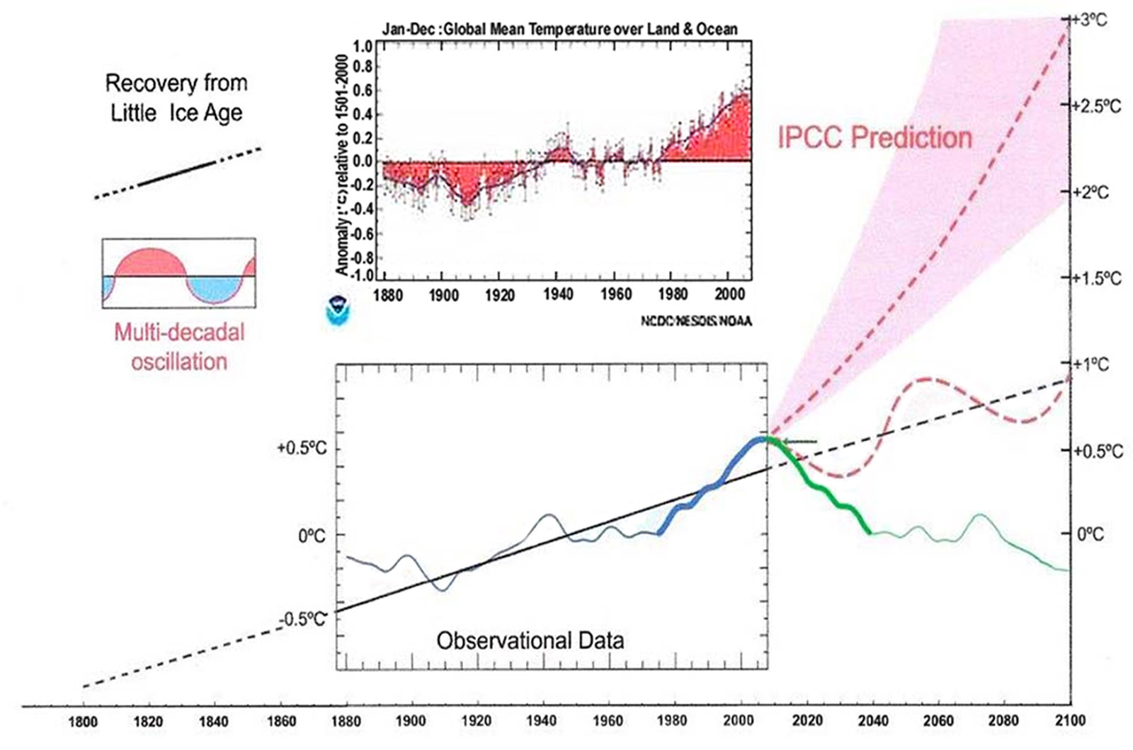
Fig. 12. Comparative Temperature Forecasts to 2100.
Fig. 12 compares the IPCC forecast with the Akasofu (31) forecast (red harmonic) and with the simple and most reasonable working hypothesis of this paper (green line) that the “Golden Spike” temperature peak at about 2003 is the most recent peak in the millennial cycle. Akasofu forecasts a further temperature increase to 2100 to be 0.5°C ± 0.2C, rather than 4.0 C +/- 2.0C predicted by the IPCC. but this interpretation ignores the Millennial inflexion point at 2004. Fig. 12 shows that the well documented 60-year temperature cycle coincidentally also peaks at about 2003.Looking at the shorter 60+/- year wavelength modulation of the millennial trend, the most straightforward hypothesis is that the cooling trends from 2003 forward will simply be a mirror image of the recent rising trends. This is illustrated by the green curve in Fig. 12, which shows cooling until 2038, slight warming to 2073 and then cooling to the end of the century, by which time almost all of the 20th century warming will have been reversed. Easterbrook 2015 (32) based his 2100 forecasts on the warming/cooling, mainly PDO, cycles of the last century. These are similar to Akasofu’s because Easterbrook’s Fig 5 also fails to recognize the 2004 Millennial peak and inversion. Scaffetta’s 2000-2100 projected warming forecast (18) ranged between 0.3 C and 1.6 C which is significantly lower than the IPCC GCM ensemble mean projected warming of 1.1C to 4.1 C. The difference between Scaffetta’s paper and the current paper is that his Fig.30 B also ignores the Millennial temperature trend inversion here picked at 2003 and he allows for the possibility of a more significant anthropogenic CO2 warming contribution.
That’s simple.
But is it realistic?
The speed of heat transfer between liquids and gases is very different. Yet the starting position affects the balance.
It must be a differential equation with an indeterminate starting position.
A mirror image seems very simple but not justifiable, to me.
Proper regression anaysis also relies fundamentally on the ‘curve’ to be ‘fitted. You can fit a linear ‘curve’ to tidal data but I don’t know why you would unless you were looking for a trend in MSL. Even then you would need to make sure you did not start your data set in a trough and finish on a crest, start and finish on crests or troughs as eiether choice would distort the result. Same thing applies to all regression analysis in that you are looking for some sort of inherent relationship but the next qiuestion is whaich relationship. Is a better fit to a line more informative than to a sine wave or quadratic? Maybe or maybe not. Worst case it is actually deceptive.
The above seems to be way above the level at which so called ‘climate science’ is conducted.
You know, if I see one more estimate of distant climate predictions, always assuming either the same atmosphere or one with higher CO2 content, I think I’ll scream. It seems as though the entire world is concerned about CO2 and attempting to reduce same. So why are these futurists ignoring all this?
I only followed about 20% of the analysis, but I noted this sentence immediately:
“As he writes, the central premise underlying the study is that climate models that are going to be the most skilful [sic] in their projections of future warming should also be the most skilful in other contexts like simulating the recent past.”
Given the stochastic nature of the system, this seems like a very shaky premise based more on wishful thinking than anything else.
Exactly, it’s equivalent to saying the future stock market is going to behave like the recent past. Complete nonsense.
Wrong, climate conditions are based on physical laws and hence predictable while the behavior of persons included in the markets are not.
A deeply technical post. Thank you Nic for digging into it. Nice work analyzing this.
I had also previously noted that the GCMs that do the “best job” of closing the TOA energy budget are the hotter running models. The modellers then have to undertake more parameter tuning to bring model ECS down to below 4 K. Before tune down they run above 5K ECS typically.
Also as Nic noted, “OLR seasonal cycle produces more skilful predictions for all predictand cases”, that result considering the cloud albedo uncertainty should set-off fundamental alarm bells about the CMIP5 models. That reduced predictors yield better skill result is likely due to the large uncertainty in clouds and related sub-grid processes that are parameterized. Nic acknowledges this by noting “unstable” which I interpret this behavior of the full set as an indication of large values in the covariances (maybe even nonlinear).
Also as a technical note, with the eigen decompositions require careful manual inspection of the results. Different numerical decomp methods can yield large discrepancies if covariance matrices are close to singular. With over-determined systems, this could be an issue. One should not let MatLab choose the method without inspection and verification.
What is clear is the current models are not fit for purpose*. They have fundamental uncertainties in basic cloud parameters that drives errors larger than the effects they are modelling (delta T of a model’s GMST due to CO2 forcing). They then tune those cloud and associated convection parameters for no other reason but to achieve an expected ECS.
* Pat Frank comes to a similar conclusion about GCMs for different reasons.
A deeply technical post. Thank you Nic for digging into it. Nice work analyzing this.
I had also previously noted on the B17 paper in last week’s WUWT thread that it is the GCMs that do the “best job” of closing the TOA energy budget that are the hotter running models. The modellers then have to undertake more parameter tuning to bring model ECS down to below 4 K. Before tune down they run above 5K ECS typically.
Also as Nic noted, “OLR seasonal cycle produces more skilful (sic) predictions for all predictand cases”, that result considering cloud albedo uncertainty should set-off fundamental alarm bells about the CMIP5 models. That fact that reduced predictors yield better skill results are likely due to the large uncertainty in clouds and related sub-grid processes that are parameterized. Nic acknowledges this by noting “unstable” which I interpret this behavior of the full set as an indication of large values in the covariances in the full set (maybe even effectively nonlinear if some covariances are >> compared to others).
Also as a technical note, with the eigen decompositions require careful manual inspection of the results. Different numerical decomp methods can yield large discrepancies if covariance matrices are close to singular. With over-determined systems, this could be an issue. One should not let MatLab choose the method without inspection and verification.
What is clear is the current models are not fit for purpose*. They have fundamental uncertainties in basic cloud parameters that drives errors larger than the effects they are modelling (delta T of a model’s GMST due to CO2 forcing). They then tune those cloud and associated convection parameters for no other reason but to achieve an expected ECS.
* Pat Frank comes to a similar conclusion about GCMs for different reasons.
something is clearly wrong if less predictors improve the fit. this caught my eye when comparing 7 vs 10 terms. mathematically there is no way 7 terms should give a better fit than 10.
the entire method is in serious doubt as the are not fitting observations. rather they are fitting the composite mean of model projections. however projections are probabilities not predictions. in effect they are repeatedly throwing a pair of dice and averaging the result to 7. then they take a large set of predictors such as the shape of the dice and speed of the throw. they curve fitting orthogonal predictors to reduce the predictor space and come up with a narrower spread that say 8 will be the next roll. but the simplest model of all says 7 is a better fit. which should not happen mathematically.
back in the real world the next roll turns out to be 2 or 5 or 12. because 7 never was a real number. it was the mean of a probability distribution. the mistake was in treating it as though it was a physical value. treating the model mean as though it was an actual observation rather than realizing it is nothing of the sort.
reducing the number of predictors should never improve the fit of the known (observed) data points. it should only improve the fit of the unknown (predicted) data points (caused by overfitting
combined with observational error). this is fundamental math. somewhat surprising peer review didn’t catch this.
but it is climate science after all. careers have be made from tree ring calibration which violates one of the fundamentals of statistics. so why should this latest result be any more surprising.
ferdberple
“reducing the number of predictors should never improve the fit of the known (observed) data points”
You would be correct in the usual case where the fit is determined using the same set of observations (here from CMIP5 GCMs, whose simulated values are treated as the observations). However, as stated in endnote [6]: ” For each GCM, ΔT is predicted based on a fit estimated with that model excluded.”
Measuring prediction error using a fit that excludes the observation for which the fit error is being measured – a “cross-validation” technique – provides a much better measure of how accurate the fit will be when applied to new observations, as the error measure is based on out of sample fits.
Here, 36 separate fits were computed, for each of the 36 GCMs, each fit being determined using “observations” from the other 35 GCMs and applied to predict the “observation” for the omitted GCM. The estimated fit error was the root-mean-square error of the resulting prediction errors for each of the 36 CMIP5 GCMs. This cross-validation based measure of fit error does reach a minimum as the number of predictor variables (here retained PLS components) increases. Beyond that point it rises again, reflecting over-fitting.
and of course this technique will only give a meaningful result if the future can be predicted from the past. and in most real world time series data this is not the case.
…
Non linearity will always make mockery of ‘the near future is like the near past’
http://vps.templar.co.uk/Cartoons%20and%20Politics/Okay.png
Is that Ken Caldeira who coined the phrase acidification of the seas and then wrote that the seas will never actually become acidic- what a guy.
While it is true that the average numbskull on the street may associate “acidification” with becoming acidic, I don’t understand why intelligent people are so hung up complaining about the use of “acidification” for becoming “less basic.”
You don’t udnerstand why the Alarmists used “acidification”? really?
I didn’t say that, and I am sure many alarmists like how scary it sounds to an ignorant public. I’ve said as much several times myself in the past.
But this notion that the term “acidification” is only correct if the pH<7 is poppycock.
This is yet again nonsense science/
The ONLY test of whether a model predicts the future is….whether it predicts the future.
Claiming it will predict the future because it predicts the past is pointless and stupid. And that’s before we wonder how tuned to the past the model is!
Phoenix44
December 16, 2017 at 9:20 am
This is yet again nonsense science/
The ONLY test of whether a model predicts the future is….whether it predicts the future.
Claiming it will predict the future because it predicts the past is pointless and stupid. And that’s before we wonder how tuned to the past the model is!
————————————–
Oh no, you missing the trick there, the real juicy dirt…….is not the ‘past’ but the “recent past”…..very big difference there dear……I think.
A model tuned to the “past” will be one that starts at ~240ppm, a lot of dT (warming) there as it gets at/to 400ppm or 460ppm.
A model tuned to “recent past” is like starting at ~380ppm or 360ppm, not as much dT (warming) when it gets at/to 400ppm or 460ppm respectively, in comparison to the “past” tuned model.
The very point where the ‘past” and the “recent past” diverge significantly, where the “past” actually stand as the past to the 280ppm reference and where the “recent past” actually stands and consist as the future to the 280ppm reference, the only point of reference that somehow still allows an approach to a dT assessment or calculation in regard to GCMs…..
And maybe I could be wrong with this…..standing to be corrected.
cheers
Not very sure, but this kind of cross-modeling seems like a new sciency and a more appealing method on averaging the models…….where the recent past approach simply a way to get the needed data for this hocus-pocus..
The proper relation of dT to the concept of proper “mean” does not exist in GCMs… GCMs can not do what is known as Trenberth “Iris”. The GCMs, seem not to be able to have or do a dT=0 for an RF mean value….
Further more the radiation imbalance always positive regardless of RF, dRF, CO2 or dCO2……or the Sun’s variability……
Two models at the same RF value, in a simulation will give or simulate different dT values if not having the same starting point.
For example, at/for an RF value at 380 ppm CO2, a model that starts from 240 will give or simulate a different dT than a model starting at 320ppm….giving a chance for exploitation when the “recent past” modus operandi
considered…….
Whatever value tried to be added by the use of the term “mean” covering the period of some years in the 21st century… that will hold no much sense as per the actual system mean point in relation to dT-RF, which actually the GCMs can not simulate, anyhow.
The system’s mean point consist as the only point to consider where the power of RF, the radiation imbalance at that power point will be related to a dT=0, no dT, the balance point of the system, in this case the atmospheric system… The only point within the dRFmax, where RF max, the point where dT will return to Zero value,,,,mathematically addressing it, as actually it means no any contribution to temps or the atmospheric thermal content beyond the dRFmax, even if RF keep going up, for whatever reason……
What I am trying to say is that when referring to dT/RF, the reality and GCMs don’t do the same, and from this kind of angle, cross-modeling as per this blog post is irrelevant……and further more,trying to calculate the natural, real dT, without considering and having the system RF “mean” point involved, aka the CO2 system mean point, within and in relation to dRF and dCO2, from my point of view, will be even more irrelevant….
Any way, I am not really sure if my comment correctly addressing the issue , as only addressing it by relying in the abstract provided and the further explanation offered in this blog post….have not checked the actual paper….
cheers
Let’s face it Gang, the models are pretty accurate at predicting climate plus or minus a couple of degrees C, at plus or minus a couple of hundred ppm CO2, even are getting the trending right plus or minus a degree per century. Not really accurate enough to make predictions of coming future deserts that the press wants to hear. A little bad that different models have quite a spread but anyway…. The program authors can be proud of their work. It’s the political ends to which the results are used that are appalling…..
Statistics is the only tool of the blind. We fancy quantum mechanics as statistical, as fundamentally unknowable, even as we ignore that gravity and the vast dark things are as yet incomprehensible to us.
We don’t need more statistics. We need more data.
and less Lore.
but given how bad/poor Data is, more Data wouldn’t really improve the show either.
I confess to not really following this paper, but taking their premise that “…climate models that are going to be the most skilful [sic] in their projections of future warming should also be the most skilful in…simulating the recent past” at face value, shouldn’t we look at the models which came closest to simulating the pause?
What do they show?
I see that the paper uses the RCP 8.5 to generate their 15% “worse than we thought” results.
Let us recall that RCP 8.5 is NOT a realistic representation of how greenhouse gases are accumulating in the atmosphere. The actual rate is much lower.
Therefore any paper which predicts temperature change based on RCP 8.5 will inevitably over-predict that temperature change
Nic.Is it not true that the harsh reality is that the output of the climate models which the IPCC rely’s on on their dangerous global warming forecasts have no necessary connection to reality because of their structural inadequacies. See Section 1 at
https://climatesense-norpag.blogspot.com/2017/02/the-coming-cooling-usefully-accurate_17.html
Here is a quote:
“The climate model forecasts, on which the entire Catastrophic Anthropogenic Global Warming meme rests, are structured with no regard to the natural 60+/- year and, more importantly, 1,000 year periodicities that are so obvious in the temperature record. The modelers approach is simply a scientific disaster and lacks even average commonsense. It is exactly like taking the temperature trend from, say, February to July and projecting it ahead linearly for 20 years beyond an inversion point. The models are generally back-tuned for less than 150 years when the relevant time scale is millennial. The radiative forcings shown in Fig. 1 reflect the past assumptions. The IPCC future temperature projections depend in addition on the Representative Concentration Pathways (RCPs) chosen for analysis. The RCPs depend on highly speculative scenarios, principally population and energy source and price forecasts, dreamt up by sundry sources. The cost/benefit analysis of actions taken to limit CO2 levels depends on the discount rate used and allowances made, if any, for the positive future positive economic effects of CO2 production on agriculture and of fossil fuel based energy production. The structural uncertainties inherent in this phase of the temperature projections are clearly so large, especially when added to the uncertainties of the science already discussed, that the outcomes provide no basis for action or even rational discussion by government policymakers. The IPCC range of ECS estimates reflects merely the predilections of the modellers – a classic case of “Weapons of Math Destruction” (6).
Harrison and Stainforth 2009 say (7): “Reductionism argues that deterministic approaches to science and positivist views of causation are the appropriate methodologies for exploring complex, multivariate systems where the behavior of a complex system can be deduced from the fundamental reductionist understanding. Rather, large complex systems may be better understood, and perhaps only understood, in terms of observed, emergent behavior. The practical implication is that there exist system behaviors and structures that are not amenable to explanation or prediction by reductionist methodologies. The search for objective constraints with which to reduce the uncertainty in regional predictions has proven elusive. The problem of equifinality ……. that different model structures and different parameter sets of a model can produce similar observed behavior of the system under study – has rarely been addressed.” A new forecasting
Last sentence above should be – A new forecasting paradigm is required
I (Patrick Brown) have responded to this critique here: https://patricktbrown.org/2017/12/21/greater-future-global-warming-still-inferred-from-earths-recent-energy-budget/
UPDATE: 12/21/17 – Dr. Patrick Brown responds here to this essay by Nic Lewis
Might be worth asking Patrick if you can put his reply up as a post here, with or without him commenting on replies.
Might need moderating.
His if you do a you get x is right, just that taking high bits of a temp data base and comparing models with high temperature biases and showing a fit does not advance science very much.
It does advance it in that it shows that having reasons for how and why you do things is important and this is what happens if you do not.
Nice to see your post.
Not happy.
” our interpretation is that the OLR seasonal cycle predictor may have just gotten lucky and we should not take its superior skill too seriously.”
You find a gold nugget and dismiss it.
Science often is serendipity and running with it.
Others with this result would say see what we have found, a great indicator, and ask why.
Oh well.
The approach taken bears a bit of the data mining problems of meta searches.
You start out with a goal in mind and find a correlation.
Yes the correlation is there but the causality is not.
Sorry, that is a bit rough , maybe you got lucky in which case I would apologise.
The sad fact is there are periods of cold in there which do not fit with any of the forecasts , but you would have to want to look for them to find them.
Nic Lewis responds at https://climateaudit.org/2017/12/23/reply-to-patrick-browns-response-to-my-article-commenting-on-his-nature-paper/