Guest essay by Dr. Antero Ollila
WUWT previously published my essay on the Semi Empirical Climate Model’ on the 21st of November. In that essay I used the term “IPCC climate model” and I received some comments saying that the “IPCC has no climate model”. I understand this argument, because IPCC should not have any models according to its mission statement.
In this essay I analyze in detail the evidence of the IPCC climate model, its properties, and its usefulness in calculating the warming values according to the IPCC science. I reckon that some readers shall also argue that there is no such thing as “IPCC science”. The mission statement says role of the IPCC…
“…is to assess on a comprehensive, objective, open and transparent basis the scientific, technical and socio-economic information relevant to understanding the scientific basis of risk of human-induced climate change, its potential impacts and options for adaptation and mitigation. IPCC reports should be neutral with respect to policy, although they may need to deal objectively with scientific, technical and socio-economic factors relevant to the application of particular policies.”
The mission statement above guides IPCC to concentrate to assess human-induced climate change issues and it means that the natural causes have a bystander role. IPCC must summarize the assessment results and to compose concise presentations based on the thousands of scientific papers. The outcomes of this work can be found in the IPCC’s reports. Finally, we have presentations like Radiative Forcings (RF) of greenhouse gases, Transient Climate Sensitivity (TCS), and Equilibrium CS (ECS). The IPCC has composed these presentations based on few scientific papers or even on its own task forces like in the case of Representative Concentration Pathways (RCPs). Therefore, it is justified to call this work “IPCC science”. It is not typically based on any individual scientific work alone, but it is based selections and combination work of IPCC.
It is true that the IPCC does not openly manifest that “this is the IPCC simple climate model”, because it would be clearly against its mission. But, it can be found in the IPCC Assessment Reports. I refer to 3rd, 4th, and 5th Assessments Reports using the acronyms TAR, AR4, and AR5. The oldest reference to the IPCC climate model can be found in TAR, chapter 6.2.1:
The climate sensitivity parameter (global mean surface temperature response dTs to the radiative forcing dF) is defined as (I have changed the Greek symbols into English ones). Equation 6.1:
dTs /dF = CSP
(Dickinson, 1982; WMO, 1986; Cess et al., 1993).
Equation 6.1 is defined for the transition of the surface-troposphere system from one equilibrium state to another in response to an externally imposed radiative perturbation. In the one-dimensional radiative convective models, wherein the concept was first initiated, CSP is a nearly invariant parameter (typically, about 0.5 K/(Wm−2); Ramanathan et al., 1985) for a variety of radiative forcings, thus introducing the notion of a possible universality of the relationship between forcing and response.
The same equation can be found chapter 2.2 of AR4 and on page 664 of AR5 in the form of equation 1 below
dT = CSP * RF
…where RF means Radiative Forcing.
The value of CSP is 0.5 K/(W/m2) according to TAR, and there is reference to the paper of Ramanathan et al. (1985). I read this paper, and I found Table 8, in which eight CSP values are tabulated from 0.47 to 0.53. One of the values was that of Ramanthan et al., and it is 0.52. The average value of these eight CSPs is 0.5. So, it looks like that the reference of TAR is not accurate. The oldest reference is to the paper of Wanabe & Wetherald (1967) and it may be the oldest reference to equation 1.
Another essential equation in the IPCC climate model is the RF formula by Myhre et al. (1989) for carbon dioxide (CO2) is equation 2 below
RF = k * ln (CO2/280)
where k is 5.35 and CO2 is the CO2 concentration (ppm). IPCC selected this equation bases on the assessment in TAR, section 6.3.5. The closest rivals were the equations of Hansen et al. and Shi. IPCC has calculated the CO2 forcing in the AR5 according to equation (2) (AR5, p. 676). The RF value of CO2 concentration of 560 ppm according to equation 2 is 3.7 W/m2. In Table 9.5 of AR5 is tabulated the same 560 ppm RF values of 30 AOGCMs (Atmosphere-Ocean Global Circulation Model also known as ‘coupled atmosphere-ocean models’), and the average value is 3.7 W/m2. It is well-known that equation (2) has been commonly used practically in all GCMs, and probably that is why Gavin Schmidt et al. (2010) calls it a “canonical estimate”.
IPCC describes its equation 6.1 like this:
Equation (6.1) is defined for the transition of the surface-troposphere system from one equilibrium state to another in response to an externally imposed radiative perturbation.
The word “equilibrium” is not a proper expression for this equation, because it could mean that this equation is applicable only for equilibrium states as defined by the specification of ECS. The basic difference between the TCS and ECS is in the positive feedbacks.
In AR5 chapter 12.4.5.1, Atmospheric Humidity there is this text:
“A common experience from past modelling studies is that relative humidity (RH) remains approximately constant on climatological time scales and planetary space scales, implying a strong constraint by the Clausius–Clapeyron relationship on how specific humidity will change.”
It is well-known that all IPCC referred climate models apply the positive water feedback and it is inherently in the value of CSP, if the value is 0.5 K/(W/m2) or greater. In ECS calculations also other positive feedbacks are taken into account like the snow and ice albedo decrease.
IPCC summarizes the differences of ECS and TCR (IPCC has changed the term TCS to TCR (Transient Climate Response)) in AR5 like this (page 1110):
“ECS determines the eventual warming in response to stabilization of atmospheric composition on multi-century time scales, while TCR determines the warming expected at a given time following any steady increase in forcing over a 50- to 100-year time scale.”
And further on page 1112, IPCC states that “TCR is a more informative indicator of future climate than ECS”. I will show later that all the IPCC calculations for future scenarios for this century are based on the TCS/TCR approach, i.e. only the positive water feedback has been applied.
In Table 9.5 are the average values of ECS and TCR of 30 AOGCMs and the values are 3.2 C and 1.8 C. According to equation 1 it is impossible to get ECS value of 3.2 K by multiplying the RF value of 3.7 W/m2 by the CSP value of 0.5 K/(W/m2) as the explanation by IPCC could insist. In Table 9.5 the average CSP is 1.0 for calculating the ECS value. The TCR value calculated according to equation 1 would be 0.5 * 3.7 = 1.85 K, which is practically the same as the average value of 30 AOGCMs. My conclusion is this: the expression “one equilibrium state to another” for equation 1 and the CSP value of 0.5 K/(W/m2) does not mean the equilibrium between the equilibrium climate sensitivity (ECS) states but equilibrium states according to TCR calculations.
We can combine equations 1 and 2 into one formula (equation 3) for CO2
dTs = CSP * k * ln(CO2/280)
If the CSP value is 0.5 K/(W/m2) and the k = 5.35, I call equation 3 the IPCC climate model. Equation 3 cannot be found in any original research paper. If somebody can do so, then I will change my mind.
IPCC has carried out the following selections:
- The elements of the equations
- The value of CSP is 0.5 K/(W/m2) (IPCC’s own value, not Ramanathan et al.)
- The RF formula for CO2 forcing.
IPCC has carried out scientific work by assessing the original research papers and selecting the elements for its model. I have done the same thing. My selection for the model elements is the same but the value of CSP is 0.27 K/(W/m2) and the value of parameter k is 3.12. It is a common practice to call my model the Ollila’s climate model and in the same way we can call the selections of IPCC to be IPCC climate model.
Even though equation 1 is as simple as possible, it is very good and accurate expression about the dependency of the surface temperature change needed to compensate the decrease of the outgoing longwave radiation (OLR) at the top of the atmosphere (TOA) originally caused by the increased absorption of CO2 concentration increase. The evidence is shown in Figure 1.

I have calculated the OLR changes using the spectral calculations applying the average global atmospheric conditions for three CO2 concentrations namely 393, 560 and 1370 ppm. There is no model applied in these calculations except the complicated absorption, emission, and transmission equations of the LW radiation emitted by the Earth’s surface in the real atmospheric conditions.
The dependency between RF change and the surface temperature change is essentially linear. This can be noticed by comparing the red curve calculated using the CSP value of 0.27 k(W/m2) to the blue curve of the spectral calculations. The TCS/TCR value of 0.6 C degrees can be read directly from Figure 1.
As shown above, the TCS/TCRds value of 1.8…1.9 C degrees is the same calculated by the IPCC’s climate model or by the AOGCMs. The warming values of RCP scenarios are originally calculated by the AOGCMs as well. IPCC tries to muddle the water by calculating the warming values of RCPs from the period 1986-2005 to the period 2081-2100, and not for the period 1750-2100 what is the specification of RCPs:
“The RCPs are named according to radiative forcing target level for 2100. The radiative forcing estimates are based on the forcing of greenhouse gases and other forcing agents. The forcing levels are relative to pre-industrial values and do not include land use (albedo), dust, or nitrate aerosol forcing.”
The warming of RCP8.5 for this period is 3.7 C degrees according to AR5 time span above. The warming from 1750 to 2000 has been 0.6 C degrees per IPCC. Thus, the total warming according to the RCP original specification from 1750 to 2100 is about 0.6 + 3.7 = 4.3 C degrees. Applying the IPCC’s climate model, the result is 0.5 * 8.5 = 4.25 C degrees, which is close enough.
The dependency between the CO2 concentration and the RF value is: RF = k * ln(CO2/280), where k is 3.12, In Figure 2, note that the equation starts from the CO2 concentration of 280 ppm onward, where the curve is slightly non-linear.

Usually I do not approve of the essential results of IPCC, but I do approve of this statement found in Chapter 6.2.1 in TAR:
“The invariance of CSP has made the radiative forcing concept appealing as a convenient measure to estimate the global, annual mean surface temperature response, without taking the recourse to actually run and analyse, say, a three-dimensional atmosphere-ocean general circulation model (AOGCM) simulation.”
Using equations (1) and (2) it is easy to calculate the TCS/TCR values (ECS values are not needed during this century and they are not real anyway) and the temperature effects of RCPs. For example, the temperature effect of RCP8.5 according to IPCC in 2100 is simply 0.5*8.5 = 4.25 C degrees, because the number 8.5 means RF value in 2100. The RF value of 8.5 W/m2 corresponds to the CO2 concentration of 1370 ppm, and according to my model the warming impact would be only 1.3 C. Eq. (1) is applicable for warming calculations, if a RF value is known. The RF values of GH gases can be calculated by equation 2, if equivalent CO2 values are known. But I do not recommend the CSP and k values of IPCC.
Why IPCC does not openly show that they have this simple climate model, which is very easy to apply, and which gives the same results as very complicated AOGCMs?
One reason could be that they are little bit shy to call it IPCC model, because they should not have it. Another reason could be that openly using it would decrease the image of climate change science, if it turns out that actually AOGCMs are not needed for calculating global warming values, which are very important in the tool box of IPCC.
There is a supposition that it is an unwritten rule among the climate change scientists that the values of the IPCC model and average GCMs should give essentially the same global values. The facts show that this is the case.
Basically the IPCC is to assess the economic and social impacts of disaster movies on a scientific basis… not determine whether there IS “global warming”… it is to *ASSUME* there is global warming and develop plans to mitigate the social and economic impacts.
So even if there *isn’t* “global warming” the IPCC isn’t allowed to say so either way.
That’s why you should ignore the IPCC.
None of that can be done without an evaluation of the magnitude of the warming!
However, it is true that people are encouraged to regard IPCC as the authority on the warming itself, which should not be the case.
Primarily the IPCC mission is to spread socialism.
Exactly! (Or at the very least, take down the nations — America in particular — enjoying the benefits of Capitalism!)
UNFCCC, Bonn, 3 March 1997
Special Session on Agenda 21: Inputs from UNFCCC
Re: IPCC
Scroll down to: March 3, 1997
Click on: EN on the right side of the webpage.
No. 5, IPCC role Agenda 21
Or follow the link on the left side of this page to other links.
http://unfccc.int/meetings/bonn_feb_1997/session/6322/php/view/documents/sort/symbol.php
IPCC / wg3
Re: Agenda 21
Working Group III: Mitigation
6.3.3.1 : Financial Resources & Agenda 21
http://ipcc/ipccreports/tar/wg3/index.php?idp=249
Correction: IPCC
Agenda 21
http://ipcc.ch/ipccreports/tar/wg3/index.php?idp=249
WHO / Bull World Health Organ: 2014, 92:774
Editorial by: Alistair Woodward
Re: IPCC and climate change
References include No.7, Naomi Klein.
http://who.int/bulletin/volumes/92/11/14-148130.pdf
http://www.who.int/bulletin/volumes/92/11/14-148130.pdf
IPCC
‘Climate Change 2014: Mitigation of Climate Change’
Chapter 7: “Energy Systems”
Select any sub-chapter.
http://www.ipcc.ch/report/ar5/wg3
IPCC
‘Working Group II: Inputs, Adaptation, and Vulnerability’
8, “Insurance and Other Financial Services”
Select any sub-chapter.
http://www.ipcc.ch/ipccreports/tar/wg2/index.php?idp=321
For the Canadian audience:
Government of Canada
Re: IPCC & Canadian Contributions
Contributors list:
http://www.canada.ca/en/environment-climate-change/services/climate-change/contribution-intergovernmental-panel/fifth-assessment-report.html
Webage has more information on IPCC and Canada with links.
IPCC, Geneva, Switzerland
History: Est. 1988
Two history brochures.
Scroll down to Brochures at:
http://www.ipcc.ch/news_and_events/outreach.shtml
The United Nations Environment Programme (UNEP) says,
The IPCC was established by UNEP and WMO [World Meteorological Organization] in 1988 to assess the state of existing knowledge about climate change: its science, the environmental, economic and social impacts and possible response strategies.. http://staging.unep.org/Documents.Multilingual/Default.Print.asp?DocumentID=43&ArticleID=206&l=en
Instead, IPCC understands its charter to be
to assess on a comprehensive, objective, open and transparent basis the scientific, technical and socio-economic information relevant to understanding the scientific basis of risk of human-induced climate change, its potential impacts and options for adaptation and mitigation. Bold added, Principles Governing IPCC Work, 10/1/1998. https://www.ipcc.ch/organization/organization_history.shtml
In its first decade and before its first Assessment Report, IPCC inserted the assumption that human-induced climate change exists, and so elevated that conjecture above comprehensive, objective, open and transparent investigation.
IPCC owns AGW (Anthropogenic Global Warming), a failed conjecture, off the bottom of the scale for science. RF (Radiative Forcing), the selected paradigm, has, as George Simpson, Head, MetOffice, told the author of the Callendar Effect (today the Greenhouse Effect) in 1938, it was impossible to solve the problem of the temperature distribution in the atmosphere by working out the radiation.
The AGW ship ran aground predicting not climate change, but its essential variable, the Equilibrium Climate Sensitivity (ECS), which instead of averaging 3ºC/2xCO2, climatologists are estimating at 0.7ºC/2xCO2, and that’s with a sign error! Better stated, its -0.7, because the conjecture and definition require CO2 to lead temperature, when in fact temperature leads CO2, as the physics requires. And IPCC climatologists don’t bother with estimating this lead/lag relationship. It was assumed away in IPCC’s interpretation of its charter.
Of course, that’s an unfair criticism, because what passes for science in academia today is Post Modern Science (PMS), the science Karl (I am not a scientist) Popper deconstructed out of Bacon’s Modern Science (MS). Popper replaced objectivity (empirical validation of predictions) with his three-pronged criterion called intersubjective testing, comprising peer review, journal publication, and consensus, each within a small, cloistered community. It’s now about voting. PMS models no longer actually need to work, and holding them to an MS criterion is denial, academically uncool.
Just briefly about CO2 and GH effect. The GH effect is real and it matches well with many scientific calculations methods. IPCC does not want to address the contribution of CO2, because they know that the most referred value 26 % of Kiehl & Trenberth is calculated in the wrong atmosphere having only 50 % of the correct water amount in the atmosphere. My figure is 13 %. When CO2 has a role in the GH effect, the increased CO2 concentration increases the GH effect unless the water has a negative feedback as proposed by Miskolczi. The direct measurements show that the long-term water content in the atmopshere is about constant and it means a neutral role of water in the cliamte change.

Aveollila: “IPCC does not want to address the contribution of CO2, because they know that the most referred value 26 % of Kiehl & Trenberth … My figure is 13 %.”
13% of what?
To Walter Sobchak . I am talking about the contributions of GH gases in the GH effect.
I hope that the IPCC does not use the symbol …. k ….. to denote ANYTHING other than Boltzmann’s Constant.
And in particular, k is NOT a variable value.
G
You mean an accurate model of the climate can be determined on a hand-held calculator? I’m sure that would depress the sale of “big iron”.
The RF values cannot be calculated by hand-held calculators. Complicated spectral analyses are needed.
That assumes the spectral irradiance flux versus time is known. It is not.
So gross simplifications must be used by the modellers.
Complicated spectral analyses then become simply WAGs without observational data.
And Models are not data. They simplify to the level they can calculate in a supercomputer runtime.
Best guess estimates are biased WAGs.
Models outputs thus become output WAGs from input WAGs.
AKA, GIGO.
WAGIWAGO!
to joelbryan. The climate change calculations are based on the yearly average values. The measured effects can be noticed in the time period of minimum 11 years (solar cycle). The radiation fluxes of the spectral calculations match with the real measurements as I have shown in a comment below.
Rocky,
Yes, in fact I recall that Willis posted about this several years ago. He showed that a simple model using the same assumptions, and running on a laptop, gave essentially the same results as the super computers costing hundreds of millions. He was careful to note that although the results were similar, that didn’tr mean they were right.
Chris
Didn’t Chris Monckton put forward a similarly simple formula a few months back?
Sure. Why not? It demonstrably works that way in some other domains. For example, you can calculate satellite orbits with considerable accuracy using simple “closed-form” equations. And, in fact, that is exactly what was done in the early years of the satellite era. Unfortunately, if more accuracy is needed, more terms are needed in the computation and the equations of motion rapidly grow in complexity. Eventually, it becomes easier to use step-by-step numerical integration — which is much more complex but scales more readily.
The climate models use numerical integration — apparently because there are no accepted closed form-equations (simple or otherwise) for climate parameters. IMO, that’s faith based science. But (perhaps fortunately) nobody but me much cares what I think.
I believe that Christopher Essex has said that underlying math is the so-called Navier Stokes Equations. If you have closed form solutions please contact the Clay Mathematics Institute so you can collect you $1,000.000 prize.
Walter — yes and no. Yes, (I think) climate modeling uses the Navier-Stokes equations which are said to describe motions of viscous fluids. But closed form equations wouldn’t necessarily have to use the same math. For example in satellite work, the closed form approximation is based on Kepler’s Laws and are basically (slightly perturbed) ellipses. Whereas the satellite numerical integration (at least that I’m familiar with) works by applying linear algebra to velocity and acceleration vectors based on Newton’s Law of Gravity.
You don’t even need a calculator. It’s not complicated – retain a little more energy and that becomes a little higher temperature. The models are pointlessly complicated, as most models are these days. As my first boss said, adding lies to a model usually just makes it spuriously accurate.
My first impression is the reason for the Climate supercomputer GCM’s, with weeks of supercomputer runtimes and large teams that spend 10,000’s manhours devising then is that they are “make work” programs for government and academia MS degrees holders and PhD degree engineers and scientists. Make work projects. Clearly.
The CO2-CAGW hypothesis is certainly an assumed log-linear output response to solar input with an assumed feedback parameter. The “Why” of all the grid and finite element climate pseudoscience analyses is to keep all those folks with employed. Duhh!!
And Dr. Antero Ollila, you must approve of our dear lost friend from Scotland’s equation too. He’s some Duke or Bishop (or Duchess, or Princess, I think) some guy we have not heard from here at WUWT in some very long time. What’s his name? Scotty? or some such.
Perhaps you are referring to Bishop Hill:
http://bishophill.squarespace.com/
Louis: I do believe Dr O’Bryan is referring to Lord Christopher Monckton of Brenchley
Was Lord Monckton’s work rejected? i have been waiting to so patiently to see how it all turned out with regard to the errors in the math etc.
Here is an example about the world of GCM development:
The Dutch climate researcher Alexander Bakker worked eight years in the Royal Netherlands Meteorological Institute developing GCMs. His job was to do something for the biases (errors) of the models, which were usually as big as the as warming values of the climate change. Finally, he lost his faith for the GCMs. He did a doctoral thesis in the Vrije University by name “The Robustness of the Climate Modelling Paradigm”, which means the functionality of climate models.
Bakker noticed two essential features, which were used as building elements of GCMs. Complicated GCMs are kept better, because they include more physical relationships and therefore more feedbacks. On the other hand, a GCM giving closest values to the old simple models, has been regarded the most reliable model! It does not sound very scientific. The basic problem in tuning a GCM is that the outgoing longwave radiation must be the same as the incoming solar radiation. Adding too much positive feedback may increase warming too much. A researcher may need a lot of creativity to keep this relationship correct. Finally, Bakker frustrated and did not want to continue this work.
Thanks for the info: I did a websearch and got a copy of his paper, and a favorable summary from Judith Curry. Your post was the jewel in this whole thread.
I think it is because people genuinely do not understand models and genuinely do not think about what they are doing. The simplest model is far more likely to be accurate and is far easier to understand, critique and change when new, better information arrives.
The idea that CSP is invariant is absolutely wrong. Radiation physics, specifically the SB Law requires that the Ts^4 relationship between temperature and emissions be honored, thus dTs/dP is 1/(4eoTs^3), which is the SB Law integrated with respect to Ts and then inverted and which has a 1/Ts^3 dependence on the surface temperature and definitely not temperature independent. Since in the steady state, total forcing is equal and opposite to total emissions across any Gaussian surface surrounding the planet, P == F, thus the steady state dTs/dP and dTs/dF are the same at each such surface. Only the equivalent emissivity, e, will be different starting at 1 at the surface whose temperature is Ts decreasing to about 0.61 at TOA.
What confuses some is that 1 calorie raises the temperature of 1 gm of water 1C, which is a linear, invariant relationship between temperature and stored energy. However; this relationship assumes that the water is receiving energy at a far greater rate than it’s radiating energy away while the Earth is radiating energy at the same rate that it’s receiving it. If the energy radiated by the Earth did not change in response to to a change in forcing, then Ramathan’s estimate of CSP would be closer to being correct. The planet responds very quickly to changes in forcing, the evidence being the difference between night and day.
The diurnal radiative forcing and the variation of the resultant surface T, I once argued was one of the primary reasons the climate change hustle of +1 or +2 deg C (or even 3 deg C) was bunk. Our planet deals with far larger swings every day in Temp than the alarmists claim is going to happen in bulk over a century. And looking at Holocene temperature time-scale, those delta T’s from models are just noise to the climate system. The GCM outputs are pure noise on a Holocene to diurnal scale.
And don’t even get me started on how much junk science the tuned GCMs outputs are to begin with.
“And don’t even get me started on how much junk science the tuned GCMs outputs are to begin with.”
Yes, I’ve studied the code and its not just garbage in/garbage out, but garbage into garbage producing more garbage.
If we talk about the absolute values, you are right that the relationship is not linear between the RF change and the surface temperature change. But the nonlinearity is so small for a change from 0 to 5 W/m2 that it has no practical meaning as you can see in Fig. 1. Also the surface temperture change from 0 to 1.3 C degree is very small thinking the Max Planck radiation law, where radiation relationship to the temperature is relative to the 4th power of T.
The calculations needed to get the radiaton changes and the surface temperature changes for compensating the increased absorption in the atmosphere, are carried out by the means of spectral calculations. They are the most accurate methods for calcutaing this phenomenon and they do apply the radiation dependency of the surface temperature. In all these calcualtions, the values of the average global atmosphere must be used.
I can show three evidences or validations for my calculations.
1) The warming effects of CO2 are always based on calculating the total absorption caused by GH gases in the atmosphere. In the clear sky conditions, the total absorption should be the same as the downward total radiation at the surface according to the Kirchhoff’s radiation law. The synthesis analysis of Stephens et al. (2012) shows an average value of 314.2 Wm-2 of 13 independent observation based studies. The value of the same flux in my calculations is 310.9 Wm-2 meaning the difference of 1.0 %. This result is not a direct validation of the correct warming value of CO2 but is rather convincing.
2) The LW radiation flux at TOA in the clear sky conditions according to the spectral analysis calculations (Ollila, 2014) is 265.3 Wm-2. According to the NASA CERES (2017) satellite observations from 2000 to 2010 this flux has been 265.8 Wm-2. The difference is only 0.19 %.
3) The error of CO2 absorption calculation code of HITRAN (2012) has been confirmed to be less than 1 % in the actual atmospheric conditions (Turner et al., 2012).
That’s true for minute changes in temperature. For a counterexample, consider New York City.
Here’s a list of average monthly temperature highs and lows.
https://www.currentresults.com/Weather/New-York/Places/new-york-city-temperatures-by-month-average.php
On average, January is the coldest month, and July is the warmest.
Average New York City temperatures
High °C Low °C
January 4 -3
July 29 20
Taking the median of average high, average low temperatures as average temperatures for the month, and you get
July 24.5 C = 297.5K
Jan 0.5 C= 273.5 K for a ratio of about 1.088 in absolute temperature, but with radiation proportional to the 4th power of temperature, you get a radiation ration of (297.5/273.5)^4 = 1.4, a HUGE increase over 1.088.
aveollila,
“But the nonlinearity is so small for a change from 0 to 5 W/m2”
The assumption of approximate linearity is just one of the flawed assumptions used by the IPCC. The climate system may be approximately linear for small, local changes, but the assumption of approximate linearity is definitely invalid across the range of temperatures found across the planet and it’s the whole planet that’s affected by forcing.
The IPCC adds confusion by calling the sensitivity an incremental metric and fails to acknowledge that all of the accumulated forcing from the Sun must have the same effect, thus the incremental sensitivity and the absolute sensitivity must be the same. The absolute sensitivity is 1.6 W/m^2 of surface emissions per W/m^2 of solar forcing corresponding to about 0.3C per W/m^2. That the incremental gain (which climate science incorrectly refers to as the sensitivity) and the absolute gain must be the same is one of the necessary conditions for Bode’s feedback analysis to be valid and that Hansen/Schlesinger ignored when fabricating their bogus feedback claims based on Bode’s amplifier analysis.
It’s absurd to think that the next W/m^2 can increase surface emissions by 0.8C corresponding to an increase in emissions of 4.3 W/m^2 while each of the 240 W/m^2 of prior forcing only added 1.6 W/m^2 to the surface emissions. If each of the 240 W/m^2 of solar forcing resulted in 4.3 W/m^2 of surface emissions, the surface temperature would be close to the boiling point of water! Moreover; the 1/T^3 dependence of the sensitivity means that the incremental sensitivity expressed as degrees per W/m^2 must be less than the average for all W/m^2 that preceded.
They add more confusion by obfuscating the Joules deficiency supporting their absurd sensitivity by expressing sensitivity as degrees of surface temperature per W/m^2 of forcing, rather than the proper, linear gain metric of W/m^2 of surface emissions per W/m^2 of forcing.
More confusion is added by referring to increased atmospheric absorption as forcing. Only the Sun forces the system and at best you can say that increased atmospheric absorption is EQUIVALENT to an increase in solar forcing while keeping the atmosphere constant. They also tend to apply the equivalent forcing to a modified system counting the effect twice. If the Sun emits nothing, no amount of CO2 will make a bit of difference to the surface temperature, thus it’s concentration can not be considered forcing. This leads to another level of obfuscation which recasts sensitivity as the effect of doubling CO2.
Yet more obfuscation arises from the bogus RCP scenarios. There are so many levels of obfuscation and misrepresentation leading to confusion, I’m not at all surprised that so many on both sides are so incredibly confused.
To CO2isnotevil. I have calculated the values in Figure 1 and it shows that the model dT = CSP * RF is really linear, and I have not used any assumptions of IPCC. I have further evidence in some comments below that this linearity works in the greater scales, too. The parameter values in my model are different: CSP = 0.27, and in the RF equation k parameter is 3.12, which means that the warming effect of CO2 by IPCC is 200 % too great.
I do not understand the forcing and gain values of yours. You have written: “If each of the 240 W/m^2 of solar forcing resulted in 4.3 W/m^2 of surface emissions, the surface temperature would be close to the boiling point of water!”
What do you mean and how do you get these figures? The average solar radiation on the Earth is 240 W/m2 and the average emitted radiation by the surface is 396 W/m2. This relationship is 396/240 = 1.65. How do you get the figure 4.3?
aveollia,
What I mean by “… boiling point of water” is that this is the consequence of all Joules being the same and the absurd sensitivity claimed by the IPCC.
The IPCC claims that the surface temperature will increase by 0.8C as the result of 1 W/m^2 of forcing. An average surface temperature increase from 288K to 288.8K increases its average emissions by about 4.3 W/m^2, thus they claim that each Joule from the next W/m^2 of forcing results in the emission of 4.3 Joules by the surface.
Each of the Joules delivered by the 240 W/m^2 of average flux from the Sun results in 1.6 Joules of energy emitted by the surface and is far less than the 4.3 Joules that the consensus claims arises from each Joule arriving from the next W/m^2 of forcing. Since all Joules are the same, if each Joule from the 240 W/m^2 of total forcing resulted in 4.3 Joules of energy emitted by the surface as the next one is claimed to do, its emissions would be 1032 W/m^2 corresponding to a temperature of 367K (94.3C).
aveollia,
Also, 396 W/m^2 at an average T of 289K is on the high side and the current 2 decade average is closer to 288K emitting 290 W/m^2 and is the value that I used.
I also agree that HITRAN is relatively close and use that for my own analysis.
I don’t agree with a value of 265.3 W/m^2 as the LWIR flux at TOA. It is closer to the 240 W/m^2 of power arriving from the Sun. You might observe 265 W/m^2 above a desert at midday with a surface temperature of 311K (38C, 100F), but as an average, it’s far too large.
To co2isnotevil. You write like this:
“The IPCC claims that the surface temperature will increase by 0.8C as the result of 1 W/m^2 of forcing. An average surface temperature increase from 288K to 288.8K increases its average emissions by about 4.3 W/m^2, thus they claim that each Joule from the next W/m^2 of forcing results in the emission of 4.3 Joules by the surface.”
Your error is that you assume that the forcing of GH gases (and other forcings, too) happens on the surface. They happen at the TOA. Therefore, the radiation change on the surface is not the same thing as the change at the TOA. IPCC’s simple model is like this dT = CSP * RF. The Csp values are 0.5 for TCS/TCR calculations and about 0.8 for ECS calculations. We can forget the CSP value 0.8, because IPCC itself do not use it for the forcings during this century. dT = 0.5 *1 = 0.5 C degrees for a forcing of 1 W/m2. My value is 0.27 C per 1 W/m2.
What?
“Your error is that you assume that the forcing of GH gases (and other forcings, too) happens on the surface. They happen at the TOA.”
You have already stated that the “forcings heat the Surface”, so how can that NOT show up as an Energy Increase (50% of overall change) from the Surface?
“Your error is that you assume that the forcing of GH gases (and other forcings, too) happens on the surface.”,
First of all, only the Sun can properly force the climate. The idea of CO2 forcing is a smokescreen where what they really mean is that increasing CO2 is EQUIVALENT to some amount of actual forcing from the Sun while keeping CO2 concentrations constant.
Solar energy does force the surface, even if absorbed by clouds, which is the only component of the atmosphere that absorbs any significant solar energy. The reason is the water cycle, where in the steady state, the energy stored in the water in the clouds can be considered equivalent to energy stored by the oceans.
The physical effect of additional CO2 in the low troposphere is to merely lower by a few feet (or inches), the thickness of a very thin layer in which all CO2 intercepted infrared is fully scattered. This has virtually zero effect on climate because convection overwhelms this process, and rapidly carries heated air upwards though the entire layer and beyond (and the same thing can be said of the largely overlapping layer in which all water vapor based IR is intercepted).
Water vapor and it’s scattering layer has some real climate effects, because energy is both stored and released in changing the state of water from gaseous, liquid and solid to the other states, and also because water also makes clouds that brighten the Earth and reflect sunlight away, thereby preventing some energy from entering the Earth’s climate system in the first place. IMO, if you want to model the Earth’s climate, you must understand clouds and water, above all.
Mickey,
Once CO2 intercepts a photon emitted from the surface, it doesn’t stop there, but re-emits it as another photon a short time later, and so on and so forth. The atmosphere is flooded photons in GHG absorption bands passing back and forth in all directions with other GHG molecules. Eventually, some of this re-transmission reaches the surface and the rest ends up being emitted into space. The idea that most of this gets ‘thermalized’ is bogus. If this were the case and that energy absorbed by GHG’s was converted into the kinetic energy of molecules in motion, there would be no photons left to make up the difference between the energy passing through the transparent window and the energy required to leave the planet for balance. Ground state gas molecules in motion have no measurable effect on the RADIATIVE balance.
The net result of this retransmission (which also includes cloud effects) does two things. First, it makes the surface warmer than it would be otherwise based on the Sun alone and second, it makes the planets emissions larger they they would be otherwise from the EM energy passing through the transparent window alone. Geometry requires that the boost in planet emissions and the return to the surface be about equal and that their sum must be exactly equal to the flux emitted by the surface and being absorbed by the atmosphere.
Regarding latent heat, what effect does evaporation and condensation have on the planets average temperature other than the effect it’s already having on the measured average temperature and their corresponding emissions?
The point here is that Trenberth screwed the pooch by including latent heat into the energy balance and returning it as ‘back radiation’, while the average temperature and it’s subsequent emissions already account for all effects that latent will have on the surface temperature. This is yet another level of obfuscation that leads to confusion on both sides.
It’s certainly true that to model the climate by modelling the atmosphere, the understanding of water is very important and no GCM has this right. However; when you treat the atmosphere as a black box with 2 boundaries (one with the surface and another with space) and conserve energy between those boundaries, the low level effects of water become moot and its net effect is simply embodied by the measured bulk behavior between the two boundaries.
That measured bulk behavior is that each W/m^2 of surface emissions results in 610 mW/m^2 of emissions by the planet and this average ratio is relatively constant across temperature, time and space and is representative of the emissivity of a gray body whose temperature is that of the surface, whose emissions are that of the planet and whose emissivity is about 0.61.
Convection starts once you have a gradient that exceeds the adiabatic lapse rate, and forces the gradient to match that rate. This limits further temperature increases to a logarithmic response, which is the familiar X degree rise per CO2 doubling as the effective radiative height increases logarithmically while the temperature gradient is pegged to a constant. At lower gradients, there is no convection, and the response is closer to a power function.
So it is wrong to say that the added CO2 has “virtually zero effect” when it is, in fact, logarithmic.
Mickey I am with you. There is a layer in the atmosphere where the temperature is equal to the graybody temperature of the earth. I believe it is about 258K, the surface being ~ 288K. That layer is not very high up. A couple of Km. The evaporation from the oceans creates updrafts that can be seen as cumulus cloud tops. They are well above the radiation equilibrium level at ~12 Km. When seen from satellites they are false colored red because they are warmer than the surrounding air. That is the missing, and important energy.
Walter,
“There is a layer in the atmosphere where the temperature is equal to the graybody …”
You’re conflating the kinetic temperature of the atmosphere, that is, the temperature based on the kinetic energy of molecules in motion, with the equivalent SB temperature based on the energy of the radiation passing through it.
Many think that equipartition of energy applies between the kinetic temperature and the radiative temperature throughout the atmosphere. This is not true and the two are largely independent, especially between TOT to TOA. The misapplication of equipartition is what leads to the flawed concept of GHG thermalization and contributes to the idea that the lapse rate dictates the surface temperature.
The kinetic temperature profile starts at the surface temperature and decreases based on the lapse rate. Once the atmosphere becomes rarefied, there are so few molecules that its temperature is irrelevant relative to the surface as its kinetic temperature increases owing to collisions with the solar wind.
The radiant temperature profile starts at the temperature of the surface decreasing monotonically until 240 W/m^2 is being emitted at TOA offseting the 240 W/m^2 of absorbed solar power corresponding to an equivalent temperature of 255K.
There are only two place where the kinetic temperature is equal to the radiative temperature. One is in the millimeter above the Earth’s surface and the other is somewhere above TOT where they coincidentally cross. Between these two point, they are roughly the same, but only due to coincidence. For example, if there were no GHG’s or clouds and only 1 ATM of N2 and O2, the kinetic temperature profile would be the same as for Earth, while the radiative temperature would be relatively constant between the surface and space as the LWIR emitted by the surface would not interact with the O2 and N2 it’s passing through.
“the water is receiving energy at a far greater rate than it’s radiating energy”
The oceans equilibrate by evaporation and using the energy to circulate their contents.
Oceans = 1000 x Atmosphere | CO2 = Atmosphere/ 2500.
CO2 is a spectator.
Walter,
The atmosphere itself is a spectator and doesn’t drive or control the climate, but is dragged along with it. Kind of like the tail of a dog.
Hasn’t Eschenbach also made a similar point here in the past?
I think the most telling observations from amongst many that the sainted Willis has made concern how much the CO2 concentration will grow in the future. Using IPCC numbers and the Bern absorption formula, it is impossible for human-induced CO2 concentrations in the atmosphere to grow by more than 70%, even if we burnt all fossil fuels on the planet this century.
From Figure 1 there are only two things laymen/laywomen need to understand.
Human CO2 (anthropogenic) emissions of all the burnable fossil fuels cannot get the pCO2 above ~900ppm. And 800 ppm is a likely high-end estimate of max by around 2150 AD (130 yrs from today). We run out of fossil fuels by then.
So,
1. Global T adds about 1.1 deg C from 2000 AD.
2. That’s about +1.9 deg C total. That’s a climate optimum for the biosphere and human agriculture.
Yes, we can live and flourish with that. Happy Days!
The new Green is more CO2. Embrace the CO2 Love.
Plants have been starving for CO2 for millions of recent years.
Mankind with returning carbon back to the biosphere has come along to save them and Gaia.
You are pretty must right. I have two papers of the CO2 circulation and the simmulations show that the atmospheric concentration will be at the level 700-900 ppm in the end of this century depending on the CO2 emissions.
Here is a blog of the residence times of the anthropogenic and the otal CO2:
https://www.linkedin.com/pulse/timescales-carbon-dioxide-atmosphere-16-55-years-nor-antero-ollila/
CO2 in AD 2100 is unlikely to exceed 600 ppm.
If we’re setting up a pool, put me down for a CO2 concentration of 571ppm in 2100. How do I come up with that? Assuming exponential growth in CO2, it has increased from (about) 315ppm in 1958 to (about) 405ppm at the start of 2018. Call that 60 years. The exponent turns out to be (about) 1.0042. So the concentration in 2100 will be 405*(1.0042**82) = 571.
When may I expect my Nobel Prize?
Nobel science prize is for published science theories not for guessing some stupid value of something at a point time. One of the betting agencies may give you odds but I will take your bet you never win the Nobel prize even if you are right.
Don K won’t win the Nobel, because he will not be alive in 2100 (unless he is well under 30 now). As for deserving it. What the heck, they gave one to Obama.
“Don K won’t win the Nobel, because he will not be alive in 2100”
Hey, that’s not fair. Climate Scientists don’t have to (and don’t) validate THEIR models. Why should I have to validate mine?
OK, just read this which makes my point rather better.
You’re assuming there will be a neutral response from natural sources and sinks to human influences?
Good luck.
dishonest Tony speaks
“It is true that the IPCC does not openly manifest that “this is the IPCC simple climate model”, because it would be clearly against its mission.”
They don’t refrain from doing that because it would be against their mission. They do it because it isn’t true, and would be stupid. Really stupid.
Equation 6.1 is a definition. They say it loud and clear. It efines a parameter relating euuilibrium states. They don’t assert that CSP is constant. You measure it (with a GCM) and find out how nearly constant it is. They say:
“Although the value of the parameter CSP can vary from one model to another, within each model it is found to be remarkably constant for a wide range of radiative perturbations (WMO, 1986).”
But there are two other big reasons why it makes no sense as a “model”
1. It relates only surface temperature to forcing. There is a great deal more to an atmosphere model than just surface temperature. But even more importantly
2. It relates only equilibrium states. Ignorant people take this formula and then say that it is a general linear relation between T and F. It isn’t. It is very clearly specified as the change you get after everything has settled down. And it never does.
That is why CSP is a diagnostic parameter. You compute it by letting a GCM run under artificial conditions for a very long time, usually making an allowance for heat flux into the sea. If it ever were a “model”, it wouldn’t be modelling anything useful.
So then people go on to say, well, easy. We’ll replace it by transient climare sensitivity, and just work out the ratio.
But there isn’t one. ECS does have the benefit of some observed near invariance, in various circumstances. TCR doesn’t at all. You define TCR in very specific circumstances – something like 1% increase compounding for 70 years. The good thing there is that the circumstances are more like what is actually happening, so a better chance of measuring it by observation. The bad thing is that the number you get has no claim to apply in other, different transient circumstances.
This obstinate misuse of a simple comment in TAR noting ancient use of 0.5 in primitive 1-D models is beyond stupid. It was a choice at the time, faut de mieux. They weren’t substantiating it, just seeing where it led. By noting that it happened the IPCC is certainly not adopting it as an official current recommendation. In fact ECS has been a central discussion in each IPCC report. The range is from about 1.5 to 4.5. In the last report, they didn’t even commit to a central estimate. Since the CSP is pretty much proportional to ECS, it’s clear that you can’t call their definition of CSP as a “model”. They don’t have a simple figure like 0.5; they have a range over a factor of 3.
If we take the approach that CSP can be anything between from 0.5 to 3, then we could not conclude what is the surface temperature in the future because of the increased CO2 concentrations. It would be impossible to say even, when the calculated increase temperature would happen: after 100 years or 500 years, when everything is settled, because the change of equilibrium values happens in the century scale.
IPCC says it simply that TCS/TCR values are applicable in shorter than century scale calculations. And I have shown that the warming values during this century for calculating TCS/TCR as well as RCP values are carried out using the CSP value of 0.5. It is simple like that. In the IPCC’s report AR5 (IPCC, 2013) TCS is between 1.0 to 2.5 ⁰C and it means the average value of 1.75 ⁰C, which is very close to 1.85 ⁰C calculated by the IPCC model (0.5*3.7 = 1.85 C).
These are my questions to Nick. TCS value means the surface temperature increase caused by the CO2 increase from 280 to 560 ppm. According to the present CO2 increase rate in the atmosphere, this would happen around 2100. What is your interpretation of TCS reported by IPCC? For me the temperature increase by 1.0 C or by 2.5 degrees means that the same result could be achieved by casting a lot. If we also assume that actually we do not know, when this increase will happen in the time scale, what is the scientific value of this kind of a model?
“What is your interpretation of TCS reported by IPCC? For me the temperature increase by 1.0 C or by 2.5 degrees means that the same result could be achieved by casting a lot.”
It’s a diagnostic. GCMs can be run under all sorts of circumstances with varying results for all sorts of climate variables. People want a summary figure that can be used to compare different models. Hence TCR, which really prescribes a standard experiment. TCR isn’t a useful way of predicting 2100 temperatures. That would be circular; GCM’s preoject the trajectories, and values of TCR are deduced from that. The variation in TCR reflects the differences in models. That is their diagnostic role.
It’s true and well known that GCM’s are not unanimous in projecting. They will improve; the alternative to a fuzzy idea of the future is no idea. In any case, the uncertainty about 2100 temperature is more due to uncertainty about what we will do to the atmosphere than to how the atmosphere will respond.
[Edited to correct the italics. -mod]
“In any case, the uncertainty about 2100 temperature is more due to uncertainty about what we will do to the atmosphere than to how the atmosphere will respond.”
Total arrogance. Thanks Nick
Nick…the science as it stand right now….says no one would know the difference
“Edited”
Thanks, mod.
“…In any case, the uncertainty about 2100 temperature is more due to uncertainty about what we will do to the ***temperature record*** than to how the atmosphere will respond…”
Fixed it.
Nick, the thing I don’t understand is that people seem to be get the same historical retrodictions and the same forward predictions using a very simple equation with the same inputs, as the hugely complicated small grid global models get.
Can you explain why this should be, and what it shows, if anything?
On the face of it, it suggests that all the detail in the models and all the computing power used is not adding much to our knowledge.
One has seen the same phenomenon in business planning. People construct hugely elaborate models with all kinds of variables accounted for in minute detail, and then when you look at the output you see that all it amounts to in forecasts is a very simple growth rate in total sales, or something similar, and that all the different scenarios can be generated by some intuitive changes to a couple of key variables.
Is this what is going on? That all the detail is simply being tuned to correspond to the simple intuitions about causation of those constructing the models, so that no matter how detailed they get, they never surprise, they always connect the inputs with the outputs in an intuitive way?
“Can you explain why this should be, and what it shows, if anything?”
It looks like a simple formula. It relates T to F. Well, T we measure. But where did the data for F come from, in this “simple” formula?
The answer is, generally, that it came from GCMs, or some similarly gridded calculation. Components may be expressed as a combination of “simple” formulae, like the log relation with CO2. But the parameters still have to be calculated. In fact the simplest way of gettig the forcings is often by back calculation from GCM outputs.
michel,
The simplest models work best at matching the past and predicting the future because there is so much uncertainty and so many presumed unknowns in the more complicated models that their results are unreliable, especially given the extreme adjustments required to get those models to match the past.
NIck,
“They do it because it isn’t true, and would be stupid. ”
So, how do you explain all the other false and stupid things that they claim in support of their destructive agenda?
Nick,
You can’t “measure” anything with a model. You can, maybe, estimate it, but then the IPCC would have to admit that nearly everything they do is an estimation with guessed at precision. And that wouldn’t sound as convincing, would it?
“You measure it (with a GCM) and find out how nearly constant it is.”
A model can’t measure anything. Measurements are made with instruments, not models. If the model depends on a parameter that it generates, you are engaged in onanism, not science.
“Measurements are made with instruments”
Well, you can’t measure climate sensitivity with a micrometer. Or even a CAT scanner (does that measure?).
hOED gives:
“2. Assess the importance, effect, or value of (something)”
with the example
“it is hard to measure teaching ability”
No instruments used there.
“it is hard to measure teaching ability”
No instruments used there.
My point stands. There is no instrument to measure teaching ability (sort of) and it is hard to measure.
Exactly. Models only do what they are told to do.
Nick Stokes
Just explain this:
http://images.remss.com/figures/climate/RSS_Model_TS_compare_trop30v4.png
And I’d love to have your opinion on this: https://climateaudit.org/2017/07/11/pages2017-new-cherry-pie/
Or this… (remember, the red line is real, black line has had “climate agenda adjustments”)

Sorry, but what is the red line exactly?
An unwelcome addition to my graph with a different baseline.
“Sorry, but what is the red line exactly?”
UAH, matched to 1979.
Javier is using one of the series which has been “adjusted” upwards to try to help the models.
No need, PAGES dont produce science, they produce outcomes.
It’s a nest of activists posing as scientists
“UAH, matched to 1979.”
Ah, I see Andy. In the red line, you’re adding a part-global troposphere satellite-based temperature model and trying to compare that with surface global temperatures, and you’re surprised they are different? And I think you already understand why that is complete nonsense, but you throw it up anyway because to you the truth doesn’t matter so much as the smear.
The satellite-based readings should have warmed faster than the surface temps. They should be an upper-limit.
“… and its uselessness in calculating…”.
There. Fixed it for you.
Dr Ollila –
?Isn’t there a weakness in the averaging assumption, and that’s why you would need GCMs to work on the finest scales possible.
From this-
“I have calculated the OLR changes using the spectral calculations applying the average global atmospheric conditions for three CO2 concentrations namely 393, 560 and 1370 ppm. There is no model applied in these calculations except the complicated absorption, emission, and transmission equations of the LW radiation emitted by the Earth’s surface in the real atmospheric conditions”
It seems to me that the only way CO2 might be able to reset the global thermostat is to work in the background where water vapour doesn’t dominate, that is, in the high, dry, areas of the atmosphere, particularly in polar regions.
Forgive me if I have misunderstood what you are trying to show
I have used the average global atmosphere for calculating the warming effects of CO2 increase. You are righ that the warming effect is much greater in the polar zones than in the tropics.
Here is a figure showing the CO2 contribution in the average global atmosphere (green shaded area), which is about 13 %
Here is the same effect of CO2 in the tropics, which is only 5.9 %

Sir, Dr. Hottel demonstrated thru experiment that emissivity of CO2 below 33 C and partial pressure of .6096 atm cm is zero. What emissivity due you apply for CO2 especially when water vapor is present?
To mkelly. I have used in spectral calculaltions the application of Gats inc. by name Spectral Calculator. They use the most common data set for GH gases by name HITRAN and its latest version, where the error with the direct measurements in the real atmospheric conditions is about 1% for CO2 I cannot tell what is the emission figure in these calculations. As I have shown in some of my comments, that the downward LW radiation and the outgoing LW radiation fluxes are very close to the measured values. In the normal science, it is an enough evidence that the model is accurate and reliable.
To Nick Stokes. You are right that the TCR are values are specidfied to use to compare different models. It means at the same time that there is an asummption that the warming value has some real meaning. The last sentence of your is: “In any case, the uncertainty about 2100 temperature is more due to uncertainty about what we will do to the atmosphere than to how the atmosphere will respond.”
That is the attitude of IPCC and the Parsi Climate agreement is based on this approach. I disagree on this approah and I will come back on this issue on some nice day.
Looking forward to reading that post aveollila!
Nick Stokes makes clear, concise criticism of the main post that is difficult to refute… John Bills and AndyG55 respond “Quick, throw up some unsourced plots that have nothing to do with the post, nor Nick’s reply! That’ll shut ‘im up!”
Although I’m quite tempted to tell you both why you’re clearly wrong, I’m not going to be distracted and play your diversion game.
My point was that the average warming values of TCS/TCR as well as the RCPs can be calculated using the simple IPCC model, which give exactly the same average values as the AOGCMs. Nick Stokes tries to muddle the water by writing that actually the CSP values varies from 0.5 to 3, which is this diversion game for me.In table 9.5 in AR5 is tabulated the average values of 30 AOGCMs and they are 0.5 and 1.0. Or is it just a pure coincidence that the simple model of dT = CSP * RF gives the same figures as AOGCMs?
Mat – entirely agree. It is a great shame that some people pile in here without too much thought. They detract from proper consideration of real issues which are raised and in my opinion devalue WUWT as a whole. People like me who have a rather tenuous grasp of some very serious points get discouraged by the flood of knee-jerk stuff and then fail to learn. No point in WUWT becoming an echo chamber for the already committed.
Nick might be at cross purposes with Dr Ollila here- I can just about see what both sides are saying-but he is an adornment to the discussion as always. He’s quick to understand and usually concise in his comments, though maybe he does rise to the bait on occasion. I do hope both he and Dr Ollila will continue to contribute.
Nick is quite good with the models and statistics. However he doesn’t understand physics and radiative transfer and so is prone to as many errors as all the commentators on here. I like Moth wish there was more discussion and less regurgitation.
The end of the day I couldn’t care a less about climate science my objection is because of the politics of the field. If we really wanted to fix the problem we could but the socialist econutt politics don’t really want to fix the problem they want to bring about a political change.
Boiling down the IPCC’s role from internationalish bableonian;
“….is to assess on a comprehensive, objective, open and transparent basis the scientific, technical and socio-economic information relevant to understanding the scientific basis of risk of human-induced climate change, its potential impacts and options for adaptation and mitigation. IPCC reports should be neutral with respect to policy, although they may need to deal objectively with scientific, technical and socio-economic factors relevant to the application of particular policies.”
Into simple sense;
“is to assess …the scientific risk of human-induced climate change …. and options for adaptation and mitigation…
… IPCC reports should be neutral although they may need to deal objectively with scientific factors relevant to the application of particular policies.”
As the first part means that the IPCC is to engage in scientific activity, the second part seems to be based on the idea that scientific ‘neutral’ language is somehow different from scientific ‘objective’ language. Is there such a thing as subjective science?
Of course, it makes sense if you add back the ‘socio-economic’ terms … which tells us that the IPCC is not about science, but propaganda. It is therefore involved in faking Science, and is no more than a literal Tower of Babel.
It might be an interesting exercise for readers to come up with their own version of the IPCC’s mission statement, and also how one might instigate a move to replace the current one.
How about “Learn how the Climate Actually Works?
1) An “intergovernmental panel” is a combination of the three last thing on Earth you would want “to assess …the scientific risk of human-induced climate change”,
* panel
* governments
* inter-,
It is single worldwide opinion by design (which is just awful in general, and even more so when it comes to risk assessment).
You can bet the very same people that are so fond of IPCC would reel at the idea of an IPVaccination or an IPDiet, imbued with the power to define policies regarding vaccination or food. And they would be right.
2) there is no such thing as “scientific risk”. There are risk assessing methodologies, each of them, AFAIK, stating in its foreword this is not science but art, requiring a great deal of common sense, even when the underlying science is solid (as HACCP for food safety, for instance). Those methodologies also are careful to distinguish the magnitude of the potential loss OR GAIN, and the probability that the loss (or gain, again) will occur.
IPCC do not even follow any of them, and does a very poor job of “could” and “may”, with “some” “confidence”.
3) GHG may be a part of human-induced climate change, but there are others. Planting forest or cutting them down, creating lakes or drying out Aral sea, draining swamp and mangroves, building dams and cities, introducing irrigation, all this change the climate. it is even meant to do so, as the water work in Seville or the huge terrace field in Asia. IPCC just don’t care about these. For instance UHI effect is one of most well known and larger climate change, affecting temperature in the 3°C magnitude, and also wind and rain pattern, in about 1% of Earth’s land surface, which is both relatively small and absolutely huge (1.5 million km², close to UK+ Germany +France). it should be the sample of all climate changes. It is not. Well, of course it is not. It is absolutely NOT scary to tell people that their climate “could” (not even sure!) change the same way it changes when they travel from rural area to the city nearby.
You left out it has the UN involved .. the most inept corrupt toothless organizations ever conceived.
right. Well, alas, only ONE of the most inept corrupt toothless organizations ever in existence (many of them still around)
Just be glad it’s toothless!
That’s a great post, despite the fact I don’t buy the idea that “equation 1” (dTs /dF = CSP) applies to real world.
For two very simple reason
1) assuming this very simple linear model has any relevancy (… ! …), since radiative wattage are in power 4 of temperature, temperature is in power 1/4 of wattage, and dT / dF is in power -3/4 of wattage so CSP is NOT constant, but reduced with higher forcing
2) almost nowhere and never are temperatures at their average world value. Given the non linearity noted above, this cannot be dismissed.
The relationship between surface temperature and the outgoing radiation change is much more complicated than the emitted radition according to the Max Planck equation, because there is also absorption by GH gases included. Figure 1 shows the results and I do believe in these calculations. It is quite easy to pinpoint one equation and to doubt that the overall situation cannot be that simple as it is. If you carry out the same calculations and show that I did somethiong wrong, then I change my opinion.
I agreed already that in absolute terms, the value of CSP is not constant but the variation is so small that it has no practical impact, see Fig 1.
I didn’t made me clear.
I don’t doubt the calculations that end into figure 1 are correct, and i’ll trust you (and others) to have correctly taken into account all relevant physical factors. That’s just radiative physic, not simple, but with solid science and scientist to have it calculated right.
What I doubt, is that radiative physics applied to average wattage and average forcing will give a correct average temperature change. I see no reason why the same 3.7 W/m² forcing (supposing this is right, and remains the same night and day, rainy or sunny, in winter or summer, everywhere on Earth…) applied in Moscow, Cairo and Brasilia (just for instance) would result in the same temperature “anomaly”, or that you can compound all of these in a single worldwide constant. Some circumstances turns wattage into higher albedo, some other into lower albedo, and this matters a lot (and other things matter, too).
A constant would make sense only if there is some reason to think every place on Earth react the same, or if know precisely enough how to compute their respective reaction to a the forcing they experience. Do we? We don’t. Actually, past variations of average temperature in recent centuries are several degrees, and we cannot even tell if they result of some forcing. They probably result of naturally occurring cycles, common in dissipative structures, a class of system atmosphere belongs to. This fact alone makes highly improbable a constant of the sort postulated.
Said otherwise, i very much doubt this “macro”, top-down way to understand climate works. And climate modelers doubt it, too, or they wouldn’t use GCM. Trouble is, they don’t even understand the climate of Brasilia, if a GHG forcing would result in lower or higher albedo, and if the extra energy (if any: the forcing could even result into LOWER energy, through not so strange albedo effect for instance) would turn into biomass, local heat, or exported to other region of the Earth, and if this exported heat will come back with some lag or not. I’ll consider changing my mind if and when someone provides some solid enough explanation for switch between glacial and interglacial, warm period and little ice age.
aveollila,
The Planck equation deals with the relationship between temperature and the emitted spectrum independent of its energy, while the Stefan-Boltzmann Law deals with the relationship between temperature and energy, independent of its frequency.
GHG’s certainly change the emitted spectrum that starts out Planck like at the surface and by the time it gets to space, it has spectral attenuation owing to GHG absorption. This reduces the total emitted power and its that reduction in emitted power that results in the lower equivalent temperature of those emissions at TOA. The T^4 relationship between the emitted power and the surface temperature is preserved and the relationship is just modified with an emissivity acting as a linear scale factor on the emitted power.
While the variability of CSP is small on either side of average, it seems to be considered as a slope passing through the origin, rather than as a slope tangent to its non-linearity as shown in the following plot.
The X axis is planet emissions and the Y axis is surface temperature. The solid lines illustrate the SB Law plotted to the same scale as the data (green -> e=0.62, black -> e=1.0) . Each little dot is the monthly average emissions of a 2.5 degree slice of latitude plotted against the monthly average temperature of that slice. The larger dots are the average over the 3 decades of weather satellite data used to produce the plot. The green line represents the measured average relationship between temperature and emissions which is about 0.3C per W/m^2. The blue line represents the IPCC sensitivity plotted to the same scale as the data. Note that it seems to be linear through the origin which is incorrect according to the actual data.
http://www.palisad.com/co2/tp/fig1.png
CO@ “lower equivalent temperature of those emissions at TOA” It is not the TOA i.e. 100 Km. It is the isothermal layer that is at the graybody temperature. That layer is much lower than TOA. Cumulus cloud tops are well above that layer.
aveollila
December 12, 2017 at 2:38 am
I have used the average global atmosphere for calculating the warming effects of CO2 increase. You are righ that the warming effect is much greater in the polar zones than in the tropics.
If what you say is true why has the overall Temperature in the Antarctic cooled at the same time that CO2 has dramatically increased?
The only “evidence” of warming over the whole Arctic is extroplation of temperatures up to 1200km away.
Even then it is very small.
Re Arctic warming this gives away the real story.
https://earthobservatory.nasa.gov/Features/ArcticIce/arctic_ice3.php
Without going deeper into this subject, the arctic temperature trend in the link above shows the same trend, which can be found in the temperatures of USA continent and Scandinavia: the temperature peak of 30s is as great as 2000s. Therefore I have composed my version about the global average temperature, which shows quite well this property but anyway the global warming since 1750 has been about 0.7 – 0.8 C degrees.
There are other cosmic forces that have increased the global temperature. Here is my earlier story:
https://wattsupwiththat.com/2017/11/21/new-study-tries-to-link-climate-models-and-climate-data-together-in-a-semi-empirical-climate-model/
The temperature increase according to SCEM from 1880 to 2015 is 0.76 ⁰C distributed between the Sun 0.35 ⁰C, the GHGs 0.28 ⁰C (CO2 0.22 ⁰C), and the AHR 0.13 ⁰C.
The temperature trend at the Antartic as well as the sea ice area have been different from the average trend of the Earth. I do not know the reasons, and it looks like the nobody else knows.
Did you look at the graph, in particular the period up to the 1930s?
Much lower CO2 and a much steeper and longer rise in Arctic temperatures.
Can I assume from your comments that you believe in CO2 Back Radiation warming the Earth’s Surface?
To TonyN. Just one example about the IPCC making science. Below is a very good presentation of the temperature trend of the Earth by Ljungqvist (2010). It shows two warm periods, which are the Roman warm period and the Viking warm period, and also the low temperatures of the Little Ice Age (LIA).

Here is the temperature graph of Mann et al. (1998) and the corrected version of McIntyre& McKitrick (a red curve).

As we know quite well, the hockey stick graph was calculated using the wrong statistical method. Another great weakness was the use of selected samples of tree-rings. Despite of these facts, IPCC selected this research paper to be the best of all hundreds of temperatures research studies and it was used to show the dramatic increase of temperature due to GH gases. It is an example in which way IPCC makes science. Now IPCC wants to forget this story, because it is a too good example, how they do science.
https://www.newscientist.com/article/dn11646-climate-myths-the-hockey-stick-graph-has-been-proven-wrong/
http://www.webpages.uidaho.edu/envs501/downloads/Nature%20Academy%20Affirms%20Hockey%20Stick%20Graph.pdf
“The report states: “The basic conclusion of Mann et al. (1998, 1999) was that the late 20th century warmth in the Northern Hemisphere was unprecedented during at least the last 1000 years. This conclusion has subsequently been supported by an array of evidence that includes both additional large-scale surface temperature reconstructions and pronounced changes in a variety of local proxy indicators, such as melting on ice caps and the retreat of glaciers around the world”.
Most researchers would agree that while the original hockey stick can – and has – been improved in a number of ways, it was not far off the mark. Most later temperature reconstructions fall within the error bars of the original hockey stick. Some show far more variability leading up to the 20th century than the hockey stick, but none suggest that it has been warmer at any time in the past 1000 years than in the last part of the 20th century.
It is true that there are big uncertainties about the accuracy of all past temperature reconstructions, and that these uncertainties have sometimes been ignored or glossed over by those who have presented the hockey stick as evidence for global warming.”
I think you saw this before,or I posted it for Tony McLeod, anyway Mann’s paper has been long shown to fatally flawed in several ways.
I see that you didn’t contest the M&M 2005 paper at all nor the Ljungqvist paper either. There are many more published papers that doesn’t support the absurd Mann paper at all,and they are truly independent from Dr. Mann’s world.
The Wegman and North Reports for Newbies
“In recent discussion of the Weblog 2007 Awards, several commenters at other blogs have argued that our criticisms of the Mannian parlor tricks have been “thoroughly refuted and discarded by climatologists, published in a credible journal”; that “other professionals in the field who also have “looked in great detail at the problem at hand” and have come to the conclusion that rather than McIntyre’s findings being “valid and relevant”, they instead have found them to be “without statistical and climatological merit”; that CA “fluffed on the whole hockey stick thing”. See for example here
Omitted in these references are the fact that the people described as “climatologists published in a credible journal” or “professionals in the field” are none other than Wahl and Ammann, serial coauthors with Michael Mann, students of Mann, who are not independent of the controversy. Indeed, they largely use (without citation or attribution or even acknowledgment to Michael Mann) arguments originally published at realclimate (and already responded to in MM 2005b(EE). Aside from their lack of independence, neither Ammann nor Wahl qualify as statistical authorities. Ammann did his undergraduate work in geology; Wahl in divinity. While this does not exclude them from having potential insight in the matter, it is evidence that one should not necessarily expect a sure grasp of mathematical and statistical issues and that their conclusions cannot be relied upon uncritically, even if Stephen Schneider accepted their article.
Readers interested in a third party view of the matter are far better off consulting the North Report, the Wegman report, (particularly) Wegman’s Reply to Questions and Richard Smith’s account of the 2006 American Statistical Association session. All of these individuals are vastly more eminent than Ammann and Wahl. Wegman, in particular, has been Chair of the National Academy of Sciences Committee on Theoretical and Applied Statistics and is a legitimate statistical expert. His comments on the Wahl and Ammann preprint are very acute and have not received appropriate consideration.
I’ve collated some of these remarks for the benefit of new readers who haven’t been following this particular story. Please read the comments below using the analogy from the previous post: see if any of our criticisms of Mannian parlor tricks have been refuted – as opposed to whether someone arguing that you can re-tool the trick to still saw the woman in half a different way. (And for this latter, pay particular attention to Wegman’s comments on Wahl and Ammann later in the post.) ”
https://climateaudit.org/2007/11/06/the-wegman-and-north-reports-for-newbies/
Well, the graph covers only 550 years, and yes it is the largest; but not by much…
http://blogs.ei.columbia.edu/2010/10/28/who-said-what-answering-ross-mckitrick%E2%80%99s-%E2%80%9Cresponse-to-misinformation-from-deutsche-bank%E2%80%9D/
““National Academy of Sciences (2006) acknowledged the merit of the critique of McIntyre and McKitrick, who identified methodological errors in the original work of Mann et al., but concluded that the primary findings of Mann et al. were not significantly impacted by these technical errors.””
“primary findings of Mann et al. were not significantly impacted by these technical errors.”
Indeed, the statistics technical error have little impact on their “primary findings” that MWP didn’t exist (just for instance), but this “finding” is crap nonetheless.
“As we know quite well, the hockey stick graph was calculated using the wrong statistical method”
In fact, your graph shows quite strong agreement between MBH and the M&M recalc. The only major diversion is in the century 1400-1500. This is not because of statistical methods, but because M&M arbitrarily excluded about half the data (Gaspe cedars), because they had 4 years missing at the start.
The ice core data exhibits an RMS temperature change in the 50 year average in excess of 1C per century over the last 11K years, so a little more than 1C per century in a shorter term average is definitely not unprecedented. If anything, contemporary change a little less than average.
“little more than 1C per century in a shorter term average is definitely not unprecedented”
Just ignoring what they are temperature changes of. An ice core measures a single location. You are comparing that with a global average. Of course individual lovations vary more. They do now too.
NIck,
The ice cores are a proxy for the temperature at the place where the water evaporated and not the temperature of where the ice core was drilled.
The also seem to calibrate the range to the expected p-p difference in global temperature expected for ice to ebb and flow.
I have low confidence in any of the absolute magnitudes of the temperatures cited for any ice core, but the relative changes are likely to be accurately represented.
Nick,
I should also point out that the variability was only measured for the most recent 10K years where the quality of the data is better and the temporal resolution is finer. I called it a little more than 1C per century since that added enough margin to cover the uncertainty. Numerically, I got a significantly larger number for DomeC and slightly larger value for the Vostok core.
“Why IPCC does not openly show that they have this simple climate model, which is very easy to apply, and which gives the same results as very complicated AOGCMs?”
Pat Frank also showed that extremely simple model gives the same results of the complicate expensive models
Extrapolation, noisy extrapolation is all these models are doing. It is impossible for these models to produce cooling trends, by design.
The relationship between surface temperature and the outgoing radiation change is much more complicated than the emitted radition according to the Max Planck equation, because there is also absorption by GH gases included. Figure 1 shows the results and I do believe in these calculations. It is quite easy to pinpoint one equation and to doubt that the overall situation cannot be that simple as it is. If you carry out the same calculations and show that I did somethiong wrong, then I change my opinion.
I agreed already that in absolute terms, the value of CSP is not constant but the variation is so small that it has no practical impact, see Fig 1.
I found one old figure, which shows the depency of radiation fluxes on the surface temperature in the average global atmosphere from -1 to 26 C degrees.

The relationships are essentially linear even within this broad temperature band. If you to think the surface
temperature band from 0 to 1.3 C degrees, which is the applicable range in the IPCC simple climate model (as well as as in my simple model) the relationships are practically linear.
I would like to say it more accurately: The temperature band from 0 to 1.3 C degrees in the simple model dT = CSP*RF, is applicable for the temperature change around 15 C degrees.
The notation of that graph appears misleading.
1. Surely the “Transmitted to space” should be Directly Transmitted to space.
2. The “Aborbed by Atmosphere” should be Aborbed by Atmosphere delaying it’s Transmittance to space.
Otherwise we really would have runaway Global Warming.
A C Osborn. Your terms are more accurate but I can say the the “transmitted radiation” in the climate science means directly transmitted to space without being absorbed by the atmosphere. The effect of absorption is that it decreases the outgoing LW radiation. The surface emits about 396 W/m2 and the LW flux to space at TOA is 239 W/2. The difference of 157 W/m2 due to the absorption does not disappear but it is transformed into heat and this energy maintains the temperature profile in the atmosphere.
That an interesting graph, I never saw before. We need to know more about it. It is of utmost importance to know whether this is a calculated graph, all things equal, or the result of an aggregation of real world measures (where and when? corrected or not for pCO2 and water daily and seasonal variation? )
I find it requires some explanation on why higher temperature results in marginally lower “direct to space” (DTS) emission. This a priori makes little sense, as higher temperature does displace the average band of emission, but still results in higher emission in all bands, so more DTS through the exit window in any case. Unless?
I also find it very interesting that DTS at 15°C looks like ~80 W/m², significantly higher (almost double) than the Earth Energy Budget values (~40~50 W/m² depending on the source). some discrepancy here.
To pagyfelyc. You read my comment carefully. I did not noticed to say that these calculations are for clear sky conditions.The results are my calculations applying spectral calculations and using the application of Spectral Calculator by Gats ins. The link to the original paper with the all-sky values is here:
http://www.jcbsc.org/issuephy.php?volume=4&issue=1
You have to look at the list of the link, and to find my paper there and then to download it as PDF version.
I think that the answer to your question, why the transmitted radiation flux does not increase, if the temperature of the emitted surface is getting higher, can be found in figure. In figure the emitted and the absorbed fluxes increase with the same rate as temperature increases. That is the explanation. The directly transmitted LW flux to space is only 28 W/m2, because clouds absorb totally the LW radiation and the average cloudeness is about 66…67 %.
To A C Osborn. I do not care to start again the conversation about the back radiation. The spectral calculations show that it exists and it is greater than the direct solar radiation at the surface: 345 W/m2 versus 167 W/m2. This situation has been confirmed by direct radiation measurements in the global scale. Denying this fact is for me like denying that the Sun does not shine. Denying would also mean that there is no GH effect in the atmosphere. Back radiation is also according to the general radiation laws.
aveollila, thank you for the response, I do not want to get into a discussion with you either.
I just wanted to establish your view of the “Sience”.
aveollila, despite your reply do you believe that the Energy absorbed by the Atmosphere DOES NOT find it’s way to space as the notation “Absorbed by Atmosphere” suggests?
To A C Osborn. The absorbed radiation does not find directly its way to space. There is a small indirect impact, because the outgoing LW radiation depends on the temperature of the outer limit of the troposphere. The theoretical temperature at the altitude of about 10 km corresponds to the Planck radiation temperature of -19 C degrees equivalent of the LW radiation of 239 W/m2. This is a simplification because the outgoing LW radiation is the sum of the atmosphere (air) emitted radiation, the directly transmitted radiation and the clouds emitted radiation. My figures for these radiation fluxes are:170 + 28 + 40= 238 W/m2 in all-sky conditions.
Well, I agree, but, still, that doesn’t make this whole “back-radiation” and “forcing” the good way to understand GHE.
I find it simpler and more accurate to start from TOA emission of ~240 W/m² ( which few variations night and day, winter and summer, sunny or cloudy) and derive surface temperature through local lapse rate (dry or wet depending on local condition). So GHE is not a matter of “forcing” and Watts, it is matter of optical depth (meters) and the amount GHG increase it (the thicker, the higher temperature on the ground).
why?
“forcing” is a way to claim that the atmosphere is a sort of insulating blanket, that more GHG turns into a better insulator. Which is wrong because
-> void is a better insulator than air, and the Moon receives just as much energy and keeps more of it because it has lower albedo than Earth, so by the insulation explanation, the Moon should be much hotter than Earth. That’s just the opposite.
-> likewise, air is a better insulator than CO2, so more CO2 should result in lower temperature. Again, the opposite.
-> Venus’ surface actually receives much less energy from the sun than Earth’s (~half of it), because higher albedo, and only have marginally better insulation than Earth (Earth’s Surface sends directly to space ~10% of its radiation, even a perfect 0% Venusian counterpart would be a mere 10% improvement), so it should colder by the insulation explanation. Doesn’t work.
-> The ultimate perfect insulator can, at most, send you back just as half the energy you send to it (and the other half must go through it). No more, short of some Maxwell’s Demon (2nd law violator). If you have a primary source that gives you E, the temperature and emissions will build up until the equilibrium where you gets E from the primary source and E from the insulator, send 2E, while the insulator receive 2E from you, from which it sends back E toward you and E to space, so that input and output seen from space are all equal to E (all equilibrium respected) . Since real measure shows that atmosphere DOES send more energy to surface than the primary source (345 Vs 167), this proves the atmosphere is NOT just an insulator: it must be more.
A heat pump, gravity- (lapse rate) and solar- powered, that pump heat toward the already hotter side (the surface), and does it with a coefficient of performance depending on the mass of fluid it works with.
This way all things add up, but “forcing” becomes irrelevant.
GH effect can be compared to be an insulator, but it does not work in the same way as the insulator in the wall construction. In the atmosphere the basic phenomena are emission, transmission, and absorption. The radiation calculations correspond to the direct measurements at the TOA and at the surface: LW flux to space about 240 W/m2, the emitted flux of the surface about 396 W/m2, and the downward flux in the clear sky condition being the same as the absorption flux. I do not find any flaws in the theory because it matches with the real world.
all insulators work the same way (impeding conduction, convection and radiation), whether wall construction, window glazing, Dewar flask, Atmosphere, or whatever. and none of them can best the perfect insulator, the one which end up at the very same temperature that the thing it insulate and with a back-radiation equal to the primary heat source.
Atmosphere DOES have insulating properties, and GHG DO increase them, but these properties DO NOT account for a greater back-radiation than a perfect insulator would. You need a heat pump for that.
“I do not find any flaws in the theory because it matches with the real world.” Well, Geocentrism also perfectly matched the real world (provided enough epicycles). A theory must match the real world, this is required, but not enough; it must also must match known findings (like the one i just recalled about insulator). Insulation GHE theory do not match FACTS about insulation
One more comment about GCMs. There are more than 100 GCMs and they all are different in some degree. The major differences are in the amount of positive feedbacks. The result can be seen in the so-called spaghetti diagrams. As I have shown the average value of TCS/TCR is practically same as the results of the IPCC simple model. The spaghetti diagrams could be produced by the simple model just by varying the CSP value. It is as good method as the selection of different feedback effects in GCMs.
aveollila
But there is only ONE “climate” on this earth. Therefore, if the 100 different global circulation models produce 100 different results, and NONE of those results resemble any decades-long real climate trends (much less the real climate particular behavior over shorter 3 and 4 year periods like El Nino and La Nina) then ALL 100 climate models are wrong.
Or, alternatively, that “1” climate model that is “right” cannot be proved correct. This reverses the Null Hypothesis: Here, we are looking for the one result that does match the experiment. And can’t find it.
Have you famioiar with my Semi empirical climate model:
https://wattsupwiththat.com/2017/11/21/new-study-tries-to-link-climate-models-and-climate-data-together-in-a-semi-empirical-climate-model/
In this model the GH gases have contribution of only about 30 % in the present temperature increase.
“as the selection of different feedback effects in GCMs”
I don’t think you have much idea about GCMs. They don’t “select different feedbacks”. They don’t deal in feedbacks at all.
To Nick Stokes. I do not have worked with GCMs. I rely on the information of IPCC. They should know the properties of GCMs quite well, right?
Once again, I refer to Table 9.5 in the latest IPCC report AR5. Here are examples tabulated in 30 AOGCMs probably, because IPCC may think that they are good examples of GCMs (minimum and maximum values in W/(m2 C)):
– Planck feedback: -3.2, not available
– Water Vapour Feedback: 1.4, 1.9
– Lapse rate feedback: -0.9, -0.2
– Surface albedo feedback: 0.2, 0.4
– Cloud feedback: -0.4, 1.2
In calculating TCS/TCR the values vary from 1.0 C degrees to 2.6 C and the average value is 1.8 C degrees. I suppose that the differences are mainly due to the degree of water feedback and possible other feedbacks. Anybody can see that the degree of different feedbacks vary from one GCM to another.
How do you explain the GCMs do not deal in feedbacks at all?
yes, you already told elsewhere that “They don’t deal in feedbacks at all”.
You just still don’t get that “feedbacks” is just the other name of action-reaction principle, basic physics.
So a model doesn’t dealing with feedbacks is just not physical. I know GMC are wrong, but not THAT wrong.
Your statement is the equivalent of a creationist carelessly stating that God never act on Earth at all.
“How do you explain the GCMs do not deal in feedbacks at all?”
The caption of that Table 9.5 is self-explanatory. It starts:
“Effective radiative forcing (ERF), climate sensitivity and climate feedbacks estimated for the CMIP5 AOGCMs (see Table 9.1 for model details). ERF, equilibrium climate sensitivity (ECS) and transient climate response (TCR) are based on Andrews et al. ( 2012) and Forster et al. (2013) and updated from the CMIP5 archive. The ERF entries are calculated according to Hansen et al. (2005) using fixed sea surface temperatures (SSTs) and Gregory et al. (2004) using regression. ECS is calculated using regressions following Gregory et al. (2004). TCR is calculated from the CMIP5 simulations with 1% CO2 increase per year (Taylor et al., 2012b), using the 20-year mean centred on the year of CO2 doubling. The climate sensitivity parameter and its inverse, the climate feedback parameter, are calculated from the regression-based ERF and the ECS. Strengths of the individual feedbacks are taken from Vial et al. (2013), following Soden et al. (2008) and using radiative kernel methods with two different kernels.”
The key words are “estimated for the CMIP5 AOGCMs”. They are calculated from the GCM results, as diagnostics. They are not part of the GCMs. They spell out how they are estimated – “using fixed sea surface temperatures (SSTs)”, “ECS is calculated using regressions”, “are calculated from the regression-based ERF and the ECS”.
“…I don’t think you have much idea about GCMs…They don’t deal in feedbacks at all…”
WTF are you talking about? Of course they do.
Example from 5 seconds of googling, from 2017…
http://onlinelibrary.wiley.com/doi/10.1002/wcc.465/full
“Abstract
Cloud feedback—the change in top-of-atmosphere radiative flux resulting from the cloud response to warming—constitutes by far the largest source of uncertainty in the climate response to CO2 forcing simulated by global climate models (GCMs). We review the main mechanisms for cloud feedbacks, and discuss their representation in climate models and the sources of intermodel spread. Global-mean cloud feedback in GCMs results from three main effects: (1) rising free-tropospheric clouds (a positive longwave effect); (2) decreasing tropical low cloud amount (a positive shortwave [SW] effect); (3) increasing high-latitude low cloud optical depth (a negative SW effect). These cloud responses simulated by GCMs are qualitatively supported by theory, high-resolution modeling, and observations…”
“Example from 5 seconds of googling”
You need to spend a minute or so reading it. Or however long it takes. It is describing how people analyse GCM output, not what GCMs do.
Here is a complete description of the workings of a NCAR GCM. See if you can find any reference to them using feedbacks, or climate sensitivity.
In my youth, I would gather with friends on the weekends to dive into fantasy role playing games of one form or another. During these elaborate campaigns, there would often be discussions about the properties of the world in which we were traveling. The discussions could become very complicated, with numerous references to obscure volumes, or precedent-setting expeditions from bygone weekends. Sometimes the arguments would involve very clever rationals and high-order reasoning. It was very impressive and a lot of fun! Eventually, the snacks would run out, our emotions would be spent, and the ability to keep our eyes open would fade. We would climb out of a parent’s basement, blinking into the early morning sunshine, trying to remember what was real and what was not!
I had the exact same feeling after reading this article and all of the responses. The IPCC is a fantasy world. It has some similarities with reality, but it is not reality. Arguments about some aspects of the IPCC virtual world can be riveting, frustrating and brilliant, but when you lift up your head and look around the real world, those arguments fade into irrelevance.
In the real world, climate changes significantly while CO2 remains essentially constant. Likewise, climate can remain constant while CO2 changes significantly. Such things are not possible in the fantasy role-playing game called the IPCC and CAGW. Reality has so much more complexity than the climate change fantasy world, that the two are not really comparable.
So lift your head from the computer screen, climb out of your parents basement, and try to recall that you live in the real world, where CO2 has never had any significant impact on climate or atmospheric temperatures, and obviously still doesn’t.
It is fun to explore fantasy worlds, but it is not healthy to stay there all the time! One can lose touch with reality and begin to believe the fantasy world is real. This always ends in disaster.
+10.
But it is all they have in their life…
… and they think their lives have “meaning” ??? !!!
Good post, jclarke341.
“It is well-known that equation (2) has been commonly used practically in all GCMs, and probably that is why Gavin Schmidt et al. (2010) calls it a “canonical estimate”.
it is used in NO GCM.
Can you elaborate on this, Steve?
well, HE has the strong position here. The burden of proof lies on those who say that equation
radiative forcing = k * ln (CO2/280)
appears in climate models.
Perhaps we should trust him, meaning, in none of these model, radiative forcing is proportionate to log pCO2.
Meaning, according Steven Mosher, none of these model follow one of the most basic findings of “settled science”.
So be it
xD
To Steven Mosher. Can you explain which formula they use for calculating the warming effect / RF of CO2? How do you explain that the simple model gives the same TCS values and the same RCP warming values as the GCMs in average? Do they use their own spectral calculations embedded in the models? That much I know that it is not straightforward preocedure, because in the real world it requires trial and error method in order to find the surface temperature increase to compensate the reduced outgoing LW radiation flux value.
10 m of air reduce IR radiation in CO2 window to 0.04 per cent. Model of warming due to photon adsorbtion and emission contains hidden assumption that all this many times repeated process is without any loss of energy. Is it possible? Can CO2 excited molecule transfer energy to other molecule?
“Can you explain which formula they use for calculating the warming effect / RF of CO2? How do you explain that the simple model gives the same TCS values and the same RCP warming values as the GCMs in average? Do they use their own spectral calculations embedded in the models?”
They use no formula for calculating the warming effect of CO2, and yes, they do their own spectral calculations. They solve the Navier-Stokes equations for flow, with associated transport of heat and constituents. Absorption and emission are solved within each element, based on gas constitution and spectral bands.
It is used in the BE volcanic/anthro model. At least in the caption. In the spreadsheet the base 10 log is used with a couple arbitrary paramemters.
This discussion reminds me of an advertising slogan by Mark Wright Disposal here in Maine: “Satisfaction guaranteed or twice your trash back.” Maybe that should be the new IPCC motto.
Dr Ollila –
Thank you very much for this well-considered post, and also for the polite and very honest way that you have responded to all the commenters here – including some who did not deserve it so much.
Your example might be followed by others, I hope.
We will look forward to your further work with great interest.
[QUOTE FROM POST]In AR5 chapter 12.4.5.1, Atmospheric Humidity there is this text:
“A common experience from past modelling studies is that relative humidity (RH) remains approximately constant on climatological time scales and planetary space scales, implying a strong constraint by the Clausius–Clapeyron relationship on how specific humidity will change.”
An assumption of constant relative humidity is a flawed assumption for calculating the warming due to an increase in IR absorption due to higher CO2 concentrations. The Clausius-Clapeyron equation is basically a theoretical curve-fit of the vapor pressure of a liquid as a function of temperature over a narrow temperature range, expressed as
dPv/d(1/T) = -Hv/R
where Pv represents the vapor pressure of a liquid at an absolute temperature T (in Kelvin), Hv is the heat of vaporization of the liquid, and R is the ideal-gas constant. Since the heat of vaporization varies with temperature, for most liquids we can get a more accurate curve-fit using the Antoine equation
Pv = exp[ A – B/(T+C)]
where A, B, and C are constants for a given liquid.
For air in equilibrium with a body of liquid water, the mole fraction water vapor in the air at 100% relative humidity is given by
y = Pv(T) / Pa
where Pv is the vapor pressure of water at temperature T, and Pa is atmospheric pressure. Since the vapor pressure Pv(T) increases with temperature, the mole fraction of water at 100% RH increases with temperature (warm air can hold more water vapor than cold air). If the relative humidity is assumed constant when the air is warmed, the warmer air contains more water vapor than the cooler air.
If the IPCC model assumes constant relative humidity while the air is being warmed by absorption of IR radiation, the additional water vapor in the atmosphere must come from somewhere. Since the Earth’s surface is 70% covered by water, this can come from evaporation of liquid water, but evaporation of water requires the air to supply about 580 calories of heat per gram of water evaporated.
Depending on the assumed original temperature of the air, heat required to evaporate water to maintain constant relative humidity can consume about 50 to 70% of the heat used to warm the air, meaning that “constant relative humidity” is a negative feedback with a coefficient of -0.5 to -0.7 on the temperature response to 1 W/m2 of IR radiation absorbed.
The IPCC is eager to claim “credit” for additional water vapor in the atmosphere for its ability to absorb more IR radiation, and supposedly amplify the CO2 effect, but they neglect the strong negative feedback of the heat required to evaporate the water.
To Steve Zell. There is something wrong in the assumption of the constant relative humidity, because it can be found only in the short-term events liken El Nino / La Nina but not in the long-term changes, see my figure on the issue. I have not found any explanation, why the atmosphere prefers the constant absolute humidity.
“If the IPCC model assumes constant relative humidity”
Goodness knows what model is now being assigned to the IPCC. There is no humidity in Dr Ollila’s. But this is a frequent distortion of the quote given
“A common experience from past modelling studies is that relative humidity (RH) remains approximately constant on climatological time scales and planetary space scales”
It is “common experience”, not an assumption. GCMs do not make global assumptions of that kind. They can’t. What they do do is to conserve mass.
Yes Nick. I agree that in GCMs they do not assume the constant relative humidity but the physical relationships show that it remains approximately constant. That is correct, and my expression was wrong. In the end, we should notice that the real atmosphere works in that way but it does not. I have calculated theoretically in two ways that the absolute water content of the atmosphere is constant. Also the direct measurements support this result not the constant relative humidity.
Link: http://www.seipub.org/DES/MostDownloaded.aspx
“…but the physical relationships show that it remains approximately constant”
But not during cloud formation which arises from air that is supersaturated with water vapour. A very non-trivial inconvenience.
The local time is now 23:09. I will come back after 10 hours and to check, if there are any new comments.
I have to apologize in advance, because I have not read and checked all comments in this blog post,and also I may be in complete misunderstanding of this blog post….but for what it could be worth……the below equation, for as far as I can tell is what I will call a paradoxical one,which lacks relevance and meaning
dT = CSP * RF
Considering dT in relation to a constant value like Rf in that equation turns all the meaning in that equation to a paradox…
That equation consist in principle as a runway warming one, but that is not the main point with it, the main point is the use of the RF value in that equation, which happens to be not a variable, when dT still a variable.
In principle the equation still will be a runway warming equation but not a paradoxical one, if RF in that one equation is swapped for dRF…..
dRF is not the same as RF……and it changes the point of that equation to a non paradoxical one.
In principle dRF= RFa -RFi where “a” in RF stands for the actual value of RF as per the actual value of the CO2 ppm concentration considered in calculating, and “i” in the RF stands for the RF initial point as per ppm initial point in consideration of CO2 ppm initial point for the equation and its calculations.
So if RF= blah..blah ( CO2/280)
dRF= blah..blah ((CO2a – CO2i)/CO2m) where “m” stands for the value CO2 as the CO2 mean…….
So for example trying to get the dRf for an actual 380 ppm point, from a starting point of 280 ppm with a supposed mean of 260 ppm, then the
dRF= blah..blah ((380 – 280) / 260)….
Now what the numbers for dT will be if dRF used instead of RF in this context????
And the main point in this is that dRF in that equation still as far as this does have some value, still it does not move that equation out of its runway warming tendency, but at the very least will make it workable and not paradoxical…
dT is not actually compatible as for and in that IPCC equation, or model, with the RF……..as far as I can tell.
And maybe I just simply being wrong with this, but hey…..please, who ever can assist and show me my wrong in this please do…. simply trying to expand my understanding.
cheers
In a way you right the the RF value referred in this equation is actually the dRF value, which has been calculated from the steady-state situation in year 1750. Because all GH gas concentrations have been increasingsince 1750, the RF value in comparison to the year 1750 have been increasing. The RF values are the used in my story in the same way as IPCC uses them. They simply marked them as RF even though they are changes from the year 1750 value.
aveollila
December 12, 2017 at 5:59 pm
Thanks for the consideration and the reply to me, aveollila.
Still there is no equality to be considered in between RF and dRF.
The “d” changes it and could not permit it, the parameter of variation…..the “d” thingy…will block an equality, or equalization between RF and dRF,as per the equation….
As I said, the equation as per my approach still not correct one at that point, but still not paradoxical,
You some how consider an equation where there the RF is straight forward given in a proper RF meaning and you still somehow strangely enough consider it as a dRF…
That in principle it can not be.
If it is RF, then it can not be considered as dRF…because this two are not the same thing……but hey in an AGWers world worms do fly…..
And as far as the dT equation stands for the IPCC point is still paradoxical..
Introducing the tester, the timer, the dt, where “t” the time, for same RF there will be different values of dT, very paradoxical as far as I can tell………That will be true for any RF value according to that IPCC equation….
dT= blah x RF x dt will give different values for dT for the same and in relation to the same value of RF in all possible ranges of RF considered,,,, a paradox…. for lack of better word…..
I am sure this is not very helpful at this point….but still…
cheers
In the original post Fig 2 is misleading, the green line representing CO2 should start at (280,0) also N2O is nitrous oxide not nitrogen oxide which could cause confusion.
Also this graph is deceptive when plotted in terms of wavelength, should be vs wavenumber (proportional to energy).
Much is wrong with Fig 2. The ranges are silly. N₂O and CH₄ are shown in ppm, with the red dot showing that they are currently on the zero axis. They will continue to stay there (in ppm); the curves are meaningless. And wrong; both (per ppm) are stronger GHGs than CO₂. And there is the question of the y axis – temperature change relative to what? For CO₂ it is at zero concentration. But for a log curve, that should go to -∞.
You are right that curves could start from 280 ppm. Anyway, the actual CO2 concentrations have been a long time over 280 ppm and therefore it has no practical meaning.
The expression of nitrogen oxide is not a specific enough and you are right, therfore, nitrous oxide is the right expression.Thanks for these corrections.
Climate models don’t work, because none account for North Korea’s glorious leader’s ability to control the weather:
http://www.smh.com.au/world/kim-jongun-controls-the-weather-north-koreans-told-20171212-h030w3.html
I found it always strange how climate scientists consider the average temperature of the Earth being given only by the atmosphere, ignoring completely the oceans in this calculation.
It is well known that the continental climate is different and colder to the climate around seas.
Attributing all the warming to the atmosphere and ignoring the oceans is an error.
“Attributing all the warming to the atmosphere and ignoring the oceans is an error.”
AOGCMs don’t do that.
“AOGCMs don’t do that.”
All warming is considered to come from the atmosphere – as explained above:
“Just briefly about CO2 and GH effect. The GH effect is real and it matches well with many scientific calculations methods. IPCC does not want to address the contribution of CO2, because they know that the most referred value 26 % of Kiehl & Trenberth …”
The oceans (water) intake heat differently to a solid object, in a way similar to a condensed atmosphere with its own GH effect. This is not modelled or taken into account to estimate why the average surface temperature is increased from 255K to 288K.
Because the ocean cover about 70 % of the Earth’s area, they have this much influence in calcuating the average surface global temperatures.
Exactly. And what is the difference between the average ocean temperature in comparison with the average land surface temperature not considering the atmosphere?
The fundamental assumption at the base of the climate consensus view is that blocking of radiated energy by radiative (greenhouse) gasses is the only factor raising the Earth’s mean surface temperatures to current levels. For the past decade, at least, there has been an alternative explanation in the thermal buffering provided by our atmosphere and ground over the daily temperature cycle.
This can be seen most simply in the DIVINER temperature data for the moon. Rather than dropping to around -270 C near the absolute zero of space, as it would if the surface was a perfect thermal insulator, it drops to around -150 C at sunset then slowly down to below -270 C over the lunar night as the ground cools. During the day it rises to around 100 C, or lower than it would if the surface wasn’t absorbing heat.
Due to the nonlinear relationship between radiated energy and temperature, E = aT^4, a temperature drop of, say, 1C during the day drops radiated energy far more than the same increase in temperature increases radiation at night. The mean surface temperature rises to regain radiative balance over the daily cycle. This is basic undergraduate physics and simple spreadsheet models give good agreement with observation.
Calculation for the Earth is more complex due to the varying nature of our surface, but simple calculations show that this effect, alone, is capable of fully accounting for our suface temperatures.
Because the GHE is not the only game in town, the original assumption needs justification. To remain plausible and scientifically valid it needs quantification. Those supporting the IPCC position need to show that the buffering effect is less than 1% of the generally accepted values of 60-100 C, and that the GHE is 200 times greater than the 0.14 C I calculate it to be.
dai
actually, “Those supporting the IPCC position” start with a non rotating and non tilting, perfectly homogeneous and flat Earth, which receive everywhere ~240 W/m² after albedo. So the buffer effect is already computed in the reference temperature 255K corresponding to these 240 W/m².
As you pertinently point out, the average temperature would be lower if the reference were alternate 480 W in day and 0 W in night.
What they miss is the fact that the atmosphere keeps the surface WARMER than a perfect insulator would (back-radiation exceed the primary solar heating, which a perfect insulator cannot do). Insulating properties do not account for that. A heat pump is needed for this to happen.
dT = CSP * RF …
is a linear equation in a system well known NOT being linear. T is known to vary with ENSO (just for instance, but many other things also come into play the same way) without any forcing.
Use it “back of envelope” is fine, just to figure out if it is worth caring.
Use it in models, however, is malpractice incarnate.
It isn’t a linear equation, unless CSP is constant, which they don’t specify. It’s a definition for CSP. And it isn’t used in models.
play-words, as usual with you.
The reference by aveollila (12/12/2017 @7:43 am) to the reality of the greenhouse effect (GHE) is irrelevant to the IPCC climate mode, the subject of his essay. IPCC divides GHE, whether real or fictional, in two: a natural part it considers to be in equilibrium, plus an enhanced part caused by human CO2 emissions modeled to produce catastrophic warming a century in the future. Both violate physics (nothing in climate is in equilibrium, [CO2] is controlled by Henry’s Law and [H2O] by the Clausius-Clapeyron Relation), but while violating physics might frustrate IPCC climatologists, in the final analysis it matters no more than the fact that its model has zero predictive power. Neither species of science, MS nor PMS, requires fidelity between models and physics or any other models: PMS requires intersubjective testing but no empirical testing, while MS requires objective testing plus fidelity to all relevant data, but nothing subjective. The two species of science are orthogonal.
Secondly, aveollila’s claim that the GH effect … matches well with many scientific calculations is peculiar on several counts. The various definitions of GHE provide nothing specific to measure. GHE accounts for the insulation provided by the atmosphere, the blanket effect, making it a consequence of infrared radiation absorption by the component gases. GHE applies to a thin blanket as well as a thick one. GHE provides no estimate of the effective thickness of the blanket, the temperature drop across the blanket anywhere, or the gas composition of the atmosphere. GHE does not specify which variables are dependent or which are independent, which are cause and which are effect. In short, the GHE is an accounting for measurements; it is not a thing to be measured.
The GHE is, of course, real. It is a vital radiation link in the thermodynamic model of the climate of a planet warmed by its sun. GHE is not sufficient, however, to estimate the surface temperature. That is precisely what IPCC attempts to do with its Radiative Forcing paradigm, which it regularly defends against unnamed and apparently unpublished (of course) critics. E.g., AR5, Ch. 8, Anthropogenic and Natural Radiative Forcing, Executive Summary, p. 8; AR4, §2.8 Utility of Radiative Forcing, p. 195. TAR, Ch. 6, Radiative Forcing of Climate Change, Executive Summary, p. 351.
IPCC’s model problems lie elsewhere than in the reality of GHE. IPCC’s model begins by holding Earth’s albedo constant, when instead it varies with global average surface temperature (GAST). And IPCC’s model then enhances the GHE by making atmospheric CO2 increase in proportion to the total of human CO2 emissions, when instead the ocean regulates the total atmospheric CO2 concentration, also in proportion to GAST. The first of these GAST feedback mechanisms mitigates temperature change from any cause, counteracting both the natural and the enhanced GHE. Because cloud albedo gates the Sun on and off, it is the most powerful feedback in climate, one again missing from the IPCC model. The second missing feedback mitigates against any CO2 emissions, natural or manmade. It removes any enhanced GHE by making atmospheric CO2 concentration an effect of surface temperature rather than a cause. Small wonder that the IPCC model doesn’t work.
aveolila (12/12/17 @ 8:06 am) claims There are more than 100 GCMs and they all are different in some degree. The major differences are in the amount of positive feedbacks. The result can be seen in the so-called spaghetti diagrams.
Q. What do you call the composite of 100 GCMs? A. A GCM.
Q. When is the composite of a lot of samples better than a single sample? A. When the samples are independent.
Q. Why is the composite of 100 GCMs no better than any one of them? A. Because IPCC has formally doctored the data into conformance with its presumption in its revised charter that anthropogenic climate change exists:
• AeroCom: Aerosol Model Intercomparison
• AMIP: Atmospheric Model Intercomparison Project
• CMIP: Coupled Model Imtercomparison Project
• MIP: Model Intercomparison Project
• PCMDI: Program for Climate Model Diagnosis and Intercomparison
• PMIP: Paleoclimate Modelling Intercomparison Project
• RTMIP: Radiative-Transfer Model Intercomparison Project
• TransCom 3: Atmospheric Tracer Transport Model Intercomparison Project
Plus these to some degree:
• GISP2 Greenland Ice Sheet Project 2
• GLODAP Global Ocean Data Analysis Project
• GPCP Global Precipitation Climatology Project
• GRIP Greenland Ice Core Project
• ISCCP International Satellite Cloud Climatology Project
• NVAP NASA Water Vapor Project
All as of AR4, Climate Change 2007.
As for spaghetti graphs, IPCC provides a remarkable example as a cover-up for its adoption of Mann’s 1999 Hockey Stick. IPCC bought the Hockey Stick in 2001. TAR, Summary for Policymakers, Figure 1(b), p. 3. http://www.ipcc.ch/ipccreports/tar/wg1/images/figspm-1s.gif
Following McIntyre & McKitrick’s 2003 debunking of the Hockey Stick, IPCC rather than retract its position, obfuscated its choice by embedding it in a spaghetti graph comprising 13 model results. AR4, §6.6.1.1, What Do Reconstructions Based on Palaeoclimatic Proxies Show? pp. 466-7, Figure 6.10(b).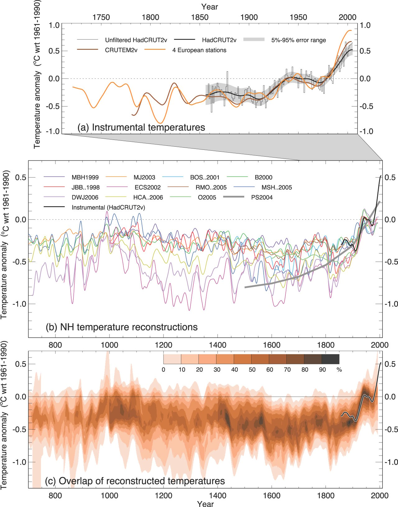
And Lo & Behold! All the reconstructions look like Hockey Sticks! Mann is rehabilitated. The reason is plain: following Mann’s methods, IPCC and the authors French-curved the data from the added reconstructions to blend the various temperature proxies into the HadCRUT2v version of the modern instrument record.
Data from biological, hydrological, and geological sources are effects accumulated over decades to eons, while the data from instrument records are accumulated over seconds to minutes. A sensor in general accumulates matter or energy from its environment into a collection aperture creating what is called a low pass filtered version of the source evolution. The acquisition process attenuates and delays the data record with respect to the input events in proportion to the integration time. As a result, events such as any segment of the temperature record of the instrument era would not even be visible in an ice core record. Appending one unprocessed record to another with a different integration time constant creates a distorted composite record. Then smoothing the transition where the records join further misrepresents the data.
IPCC’s methods here are just a few examples of the many forms of junk science practiced by IPCC. But for the wasted treasury, the political disruption, the resulting human suffering, and the damage to scientific credulity, IPCC is a laughing stock.