By Andy May
Last week, I posted a global temperature reconstruction based mostly on Marcott, et al. 2013 proxies. The post can be found here. In the comments on the Wattsupwiththat post there was considerable discussion about the difference between my Northern Hemisphere mid-latitude (30°N to 60°N) and the GISP2 Richard Alley central Greenland temperature reconstruction (see here for the reference and data). See the comments by Dr. Don Easterbrook and Joachim Seifert (weltklima) here and here, as well as their earlier comments.
Richard Alley’s (Richard Alley, 2000) central Greenland reconstruction has become the de facto standard reconstruction and is displayed often in papers and posts. And, truth be told, I’ve often used it. See here for an example. But, it is a central Greenland reconstruction, uncorrected for elevation differences over time, and all of Greenland is north of 60°N. A better comparison is with my Arctic reconstruction that goes from 60°N to the North Pole. This comparison is shown in figure 1.

Figure 1
Alley’s reconstruction is based upon trapped air in ice cores taken from central Greenland and his proxies are calibrated to air temperatures on land. My Arctic reconstruction is based upon nine proxies, five are marine proxies and 3 are land proxies. Only one of the land proxies is a Greenland ice core and I used a composite of two Greenland area ice cores, Agassiz and Renland, by Vinther, et al. (2009) and not the better-known Alley reconstruction. The Vinther reconstruction and the Alley reconstruction are compared, using actual temperature, in figure 2.

Figure 2
As can be seen in figure 2, the Vinther Agassiz and Renland reconstruction is less erratic and has a more prominent Holocene Climatic Optimum (HCO) than the Alley reconstruction. In addition, the Vinther Medieval Warm Period is older and the Roman and Minoan Warm periods are far less prominent and offset in time. Notice the reconstructions match in the Little Ice Age (LIA) and that the Vinther Holocene Climatic Optimum (HCO) from 8000 BC to 4500 BC is more prominent. The HCO doesn’t really show up in the Alley record. Below we compare our Arctic reconstruction to the Vinther record in Figure 3.

Figure 3
Vinther’s record shows a more prominent HCO than ours, more detail and a deeper LIA. Finally, let’s compare both Vinther and Alley to our Northern Hemisphere mid-latitude reconstruction in figures 4 and 5.
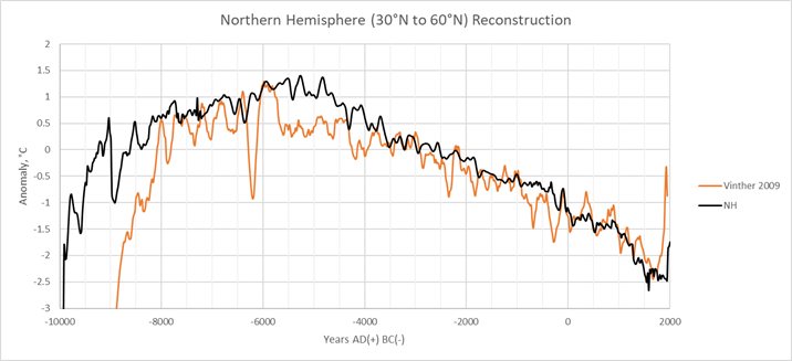
Figure 4
It is interesting that Vinther agrees with the mid-latitude Northern Hemisphere reconstruction in the Neoglacial period (roughly 5700 BP or 4300 BC to the present), but agrees better with the Arctic reconstruction during the HCO. I’m not completely sure why that is.

Figure 5
Comparing figure 4 to figure 5, we can see that Alley has a very flat trend and is more active than Vinther. Vinther is a better match to our Northern Hemisphere mid-latitude reconstruction. Alley’s reconstruction starts to show the HCO and then fizzles at about 1,000 years in to it. Figures 4 and 5 are anomalies from the mean temperature from 9000 BP to 500 BP, however, which distorts the picture a bit given the two reconstructions differ on the temperatures of the HCO and the LIA. I refer you to figure 2, where we compare Vinther to Alley in actual temperature and not in an anomaly form. Here the two reconstructions agree on the temperature of LIA, but the Alley reconstruction does not see the HCO. We see that the key difference between the two is the degree of warming during the HCO.
Why are Alley and Vinther different?
The short answer is that Vinther, et al. (2009) corrected their ice core records, including GISP II and GRIP, for elevation differences and Alley did not. In Vinther’s words:
“The previous interpretation of evidence from stable isotopes (δ18O) in water from GIS [Greenland Ice Sheet] ice cores was that Holocene climate variability on the GIS differed spatially and that a consistent Holocene climate optimum—the unusually warm period from about 9,000 to 6,000 years ago found in many northern latitude palaeoclimate records—did not exist. Here we extract both the Greenland Holocene temperature history and the evolution of GIS surface elevation at four GIS locations. We achieve this by comparing δ18O from GIS ice cores with δ18O from ice cores from small marginal icecaps [Agassiz and Renland]. Contrary to the earlier interpretation of δ18O evidence from ice cores, our new temperature history reveals a pronounced Holocene climatic optimum in Greenland coinciding with maximum thinning near the GIS margins. Our δ18O -based results are corroborated by the air content of ice cores, a proxy for surface elevation.”
In figure 6 we see a summary of the Vinther, et al. (2009) data, it is their figure 1.
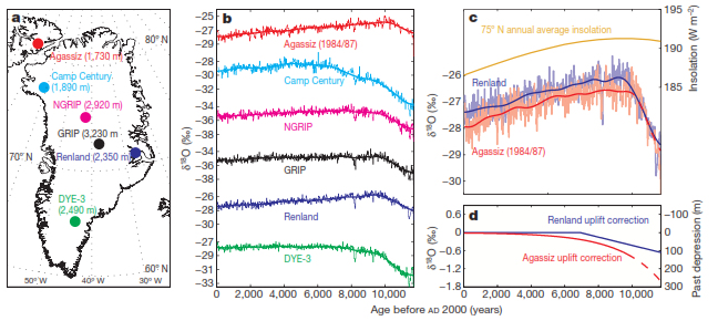
Figure 6 (Source: Vinther, et al. 2009)
The six cores are well distributed across Greenland, with Agassiz on Ellesmere Island very close to Greenland. Agassiz and Renland are both coastal cores and have similar profiles. It is possible to reconstruct the elevation histories for these two locations with confidence, so they are used to develop corrections for the remaining 4 ice cores. All six core records shown were included in the Vinther, et al. (2009) reconstruction after adjustment for elevation and ice thickness changes, but the Agassiz and Renland cores are the key cores. The corrections to these cores are shown in 6D. The δ18O profiles for these cores, after the uplift (or elevation) correction has been applied, is shown in 6c. Considering that Agassiz and Renland are on opposite sides of the GIS and 1,500 km apart, the agreement between the two corrected records is astounding, as Vinther, et al. (2009) described it in their paper.
Alley’s reconstruction focused on the GRIP and GISP II cores, these two cores are 30 km apart in central Greenland, they are combined into one point called GRIP in figure 6.
Below is a better location map for the Greenland ice cores, shown as figure 7.
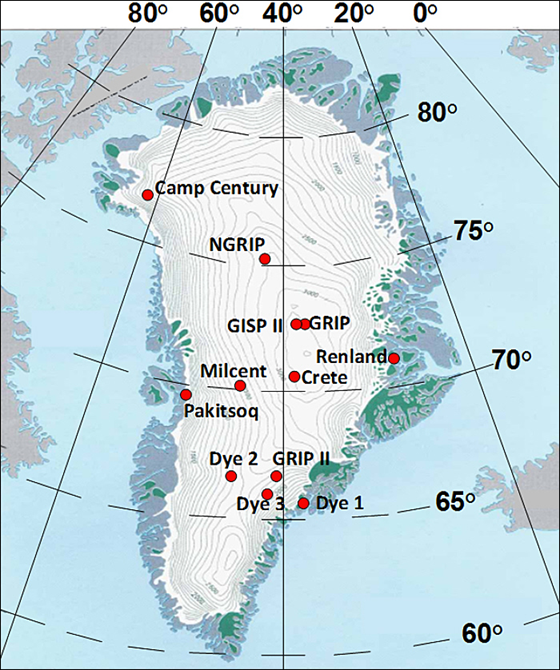
Figure 7 (Source CDIAC)
Temperature determination in these ice cores is done with a function of δ18O and it has been shown by Johnsen and White (1989) that the average δ18O level over and around the Greenland Ice Sheet (GIS) is almost completely described by altitude (-0.6‰/100m) and latitude (-0.54‰/degree N). The altitude effect is due to the moist-adiabatic cooling of an air mass rising above the GIS. As it cools, precipitation and fractionation take place. There are more details on this in the Vinther, et al., 2009 supplementary materials. Thus, there is a sound basis for building a good δ18O temperature record if the altitude of the ice surface is known throughout the Holocene. Elevation differences must be taken into account. As Vinther, et al. (2009) write:
“… the differences in the long-term δ18O trends seem to be related to changing GIS elevation …”
The Holocene Climatic Optimum was a warm period and it caused melting of the GIS. Thinning at the Camp Century and DYE-3 sites started very soon after the HCO began over 9,000 years ago. The thinning progressed from there to the GISP II/GRIP location in a few thousand years, certainly by 6,000 BP. This affected the GISP δ18O temperature record and all but eliminated the HCO response that we see in other Northern Hemisphere records. The elevation corrections applied to the four sites, including GRIP, NGRIP and GISP II are shown in figure 8, from Vinther, et al. (2009).

Figure 8
The Camp Century and DYE-3 locations are on the coast and they are affected most. In the interior GRIP and NGRIP locations (remember GISP II is next to GRIP, see figure 7) the effect is less, but still significant.
Conclusions
If we accept the work that Vinther, et al. (2009) have done as being correct, and I see no problems with it, then the Aggasiz-Renland δ18O records, after correction for elevation records are correct. These records are 1,500 km apart and on opposite sides of the GIS, thus the temperature record of Greenland for this period must be fairly uniform for this period of time. Because of the geological conditions at the Aggasiz and Renland sites, their elevation histories can be reconstruction with some confidence as explained in Vinther, et al.’s paper and supplementary materials. Given that we also know the controls on the average δ18O with confidence, then we can provide a reliable temperature record for these sites. This is the record used in my Arctic reconstruction and the other 8 records used in the reconstruction agree fairly well.
Vinther, et al.’s reconstruction also agrees well with my Northern Hemisphere reconstruction from 4,000 BC to the present. It reaches a lower temperature extreme in the HCO, but matches the HCO of my Arctic reconstruction. Generally, I prefer the Vinther et al. reconstruction to Alley’s earlier GISP II reconstruction for the purpose of detecting the major climatic events of the Holocene and estimating the difference between HCO temperatures and LIA temperatures.
However, for locating climate events in time and whether the event is a warming event or a cooling event, using a single ice core proxy, that is well dated is fine. And the dating error in ice cores is very low, less than 1% (Alley, 2000). It is just that the magnitude of the temperature swings are probably incorrect in the GISP II and GRIP cores due to elevation changes as Vinther, et al. have shown. These changes (or errors in temperature) are the most severe in the HCO. This problem affects the magnitude of the estimated temperature but not the timing of the events.
Using multiple proxies, as I have, helps measure a more accurate and robust temperature anomaly for a region or the whole globe, but adversely affects the timing of events due to averaging multiple proxies with possibly inaccurate dates. Dating errors of 100 to 150 years are probably common and when averaging records with this sort of error, there will be loss of short term amplitude and problems estimating the timing of major events. This always needs to be considered in this sort of work. Amplitude reduction or excessive smoothing of the temperature reconstruction can be minimized by using fewer proxies, higher resolution proxies (shorter sample intervals), minimizing the proxy drop out at both ends of the reconstruction by avoiding short term proxies, and selecting proxies that are not overly affected by local events or local geology. Careful proxy selection is critical for a robust record, for more details on proxies to be avoided and proxies to include see my posts on the reconstructions I made. The final post, which will lead you to the others is here.
So, what is the purpose? Do you want to know, as accurately as possible, when a Northern Hemisphere warming event or cooling event occurred? Then using GISP II or GRIP will work best. Do you want to estimate the average temperature change during the event? Then I would recommend my reconstructions, but realize that the estimate may be conservative and the date of the event may be incorrect by 100 to 150 years. Our knowledge and data about Holocene temperatures are limited, but by using what we have wisely we can begin to get our arms around it.
Excellent…thanks Andy
Yes, totally agree…it’s good to have some light shone on this rather confusing subject.
Nice work on proxies.
I’d like to hear your explanation as to why the Greenland ice cores are considered a Greenland proxy rather than a global or at least hemispheric proxy. Doesn’t the O18 temperature dependence relate to the sea surface temperature Shouldn’t the O18 (or H2O18) have been well mixed in the atmosphere? Wouldn’t that mean that O18 levels represent the global ocean temperature, not local temperature?
I can understand the reasoning as to why there are elevation differences, but that still doesn’t mean that this is a local phenomenon.
Remember that 18O/16O fractionates each time there is a phase change — not just in ocean evaporation, but also any time part of that moisture produces rain or snow, and when snow forms over Greenland. So the overall fractionation is a complex process. Typically, for a given site over reasonably short time periods, it is assumed that the moisture source and temperature remain constant. Thus, fractionation in the Greenland region would dominate. And, different elevations could induce different partial rain-snow events.
Andy, this was an interesting comparison, Vinther modified the proxies by adding
or subtracting numbers to his liking, what he considered “Elevation change”, And
because supposedly elevations went up or down by 10 m or 50 m, then the climate
(temps) got warmer or colder….???
There are temp high peaks in Alley, whereas for the same
event there are low temp peaks in Vinther…..
And here we get closer to the problem, we need to carry out a PEAK/SPIKES –
comparison. And there are 2 approaches:
1. The small peak method: In Alley there are DISTINCT 62-yr CYCLIC PEAKS for all
the Holocene, starting 5600 BC. This is the accuracy test: If they appeared in Vinther,
then Vinther would be OK. but I am confident, that the 62 yr. cyclicity is NOT in Vinther….
2. The large peak method: I am just doing a new paper, showing that 13 named cosmic
meteor impacts within the Holocene (dated +/- 10 years) produce, depending on
meteor size, a period of global cooling (decadal to centennial): Small bolide impact –
shorter, less deep cooling period, larger bolide (i.e. crater size) impact – longer and
steeper cooling. I will hand in the paper for peer-review this year, it is almost ready.
Now, Alley EXACTLY matches meteor impact dates and cooling periods according to
crater sizes. If your reconstructions do not show impacts and crater sizes, then
they blurr the climate evolution following each of the 13 meteor impacts, thus being
not correct.
All cooling periods are known and described in many Holocene papers. – some cooling
periods were VERY GRAVE and the reconstructions, especially those from deep
ocean proxies, retard and belittle the partly catastrophical cooling events (it is cosier
at the bottom of the sea, whilst above the water the ice storms were howling).
And to Vinther: If he puts a warm spike, where a cooling period should be,
, then he is entirely mistaken with his “Elevation changes – climate changes”.
Se more in http://www.knowledgeminer.eu/climate-papers.html.
Joachim, I think in terms of timing events Alley might be better. But, in terms of magnitude (or amplitude) of each event, Vinther is better. The elevation changes during the warm HCO were large and they had a big effect.
Andy,
Since age calibration always includes a substantial error, isn’t there a good chance that the magnitude (amplitude) of multi-proxy reconstructions has been muted, relative to single-proxy reconstructions?
David, Yes. But, the GISP/GRIP ice core profile is distorted by GIS elevation changes and that wiped out the HCO (Holocene Climatic Optimum) in those reconstructions. My reconstruction gets the shape right and restores the HCO, plus it covers more than Greenland. But, short term amplitude (<150 years or so) is reduced. If you want to use a Greenland reconstruction, the Vinther, et al. Agassiz-Renland elevation corrected one is the one to use. But, it only represents the Greenland area, which is anomalous relative to the rest of the world. At least it shows the HCO.
Vinther shows a 3.5 degree difference between the HCO and the LIA, my NH reconstruction shows the same, but slightly offset in time. Is the time difference between Greenland and the rest of the northern hemisphere? Or is it due to averaging proxies? Don't know. But, I think I'm getting the large scale magnitudes correct, the magnitudes of short term events? Probably not.
My Arctic reconstruction shows a 2.5 degree difference, is this because it covers a larger area? Or because of averaging too many proxies? Not sure. In the Northern Hemisphere, I suspect 3.5 degrees is correct, but for the whole world, probably 1.5 degrees is correct.
If your hypothesis rests or requires a single proxy, you are on shaky ground. GISP2 is known to contain periodicities that are not found elsewhere.
I’d never thought of an elevation correction for Greenland cores. With the small temperature range we’re working with, that’s a significant difference.
Accuracy vs averaging
The data in this paper consists of two very different types: (1) specific data from a single locality (e.g., GISP2), and (2) composite averages of several different proxies at multiple localities. There are important differences in these types of data. For example, if you want to measure the chemistry of water and you have two buckets, one with pure distilled water and another with impure water, you could combine the two so you are using all the water you have, but in the process, you destroy the good data you could get from the distilled sample, ie. averaging of the two samples destroys the accuracy of the pure sample. If you put one foot in hot coals in a fireplace and the other foot in a bucket of ice, the average temperature would suggest a comfortable temperature, but it doesn’t represent the temperature of either of your two feet. The same is true of any averaged data.
Andy’s curves represent composite data, including different proxies at multiple localities. As I pointed out in a comment on his previous paper, from 5000 years ago, the Northern Hemisphere (yellow) curve shows monotonic cooling with only minor temperature bumps until about 1000 years ago. In contrast, the GISP2 core shows 7 warm spikes from about 4500 to 1500 years ago and the trend line is essentially flat—at the end of the Roman Warm Period (~1500 yrs ago), the temperature was essentially the same as it was 4500 years ago. The GISP2 temperature then drops abruptly into the Dark Ages Cool Period for several hundred years before warming again during the MWP (~1300 to 900). The NH (yellow curve) shows none of this. The Roman Warm Period, Dark Ages Cool Period, Medieval Warm Period, and Little Ice Age are all well documented historic climatic changes. No matter what you think of the GISP2 temperature curve, historic records confirm that the temperature variations in the core really happened, so the question becomes how valid is the NH (yellow curve) that shows none of them?
Andy’s Fig 1 shows the GISP2 curve plotted with his Arctic composite curve of 5 marine proxies and 3 land proxies (i.e., averaged). They are quite different—the Artic curve, like the NH curve, is essentially montonic except for a deep cooling at about 7,000 years that corresponds to a warm spike in the Alley curve, and the Little Ice Age. The deep cooling at 8,200 years is much subdued in the Arctic curve, neither of the two pronounced warm spikes in the Alley curve at about 8,000 and 7,000 years show on the Arctic curve, none of the warm and cool periods of the past 6000 years is discernable, and the sharp drop of temperature into the Little Ice Age at 1500 years ago does not show at all.
Fig 2 is a comparison of the Alley curve with a curve by Vinther. It’s even worse—it shows essentially monotonic cooling thru most of the Holocene from 8,000 years ago to recently with none of the post-7000 year warm/cool periods discernable. The Vinther curve does show higher early Holocene temperatures. Andy says “Using multiple proxies, as I have, helps measure a more accurate and robust temperature anomaly for a region or the whole globe.” I would argue just the opposite—the most accurate temperature is the GISP2 curve (Cuffy and Clow’s curve, Alley’s curve, and the δ18O curve). I would also argue that averaging destroys accuracy (as in the case of putting your feet in coals and ice and averaging the temps).
Dr. Easterbrook, The real problems with the GISP record is it misses the HCO which shows up in almost every other reconstruction and proxy. The HCO is also very well documented in glacial records and in marine proxies around the world. Look at the tropics reconstruction in part 2 of my series, this represents 50% of the Earth’s surface. Vinther describes the geological setting for the Agassiz and Renland ice cores very well in his supplemental materials and they are the best ice core records, they have an HCO also. See figure 6 above.
The HCO does exist, why doesn’t GRIP/GISP II show it? It is loss of elevation during the HCO.
I do not doubt the timing of the events in GRIP/GISP II, but that does not mean the magnitude of the events is correct.
If you look carefully at figures 2 and 3 you will see that the same events are in both, but they are sometimes offset in time a little. I suspect the GISP II/GRIP times are correct, but the magnitude is off. Plus the shape of GISP II/GRIP is off as the Greenland Ice Sheet is shifting and the HCO is eliminated.
In looking at the GISP2 data, I’m not convinced that it ‘misses’ the early Holocene warming. The warm peaks of the early Holocene in GISP2 are up to 5 F warmer than today and if it weren’t for two deep cooling spikes, the early Holocene would stand out as the warmest part of the Holocene. Therefore, I don’t see the rationale for saying GISP2 ‘misses’ the early Holocene warming.
Your problem is that GRIP is from 30 km away from GISP2 and doesn’t show the same periodicities and features as GISP2.
So the question is: Why do you think you should use and relay on GISP2 instead of GRIP? According to you both have the same accuracy at displaying temperature changes, yet the conclusions are not the same. Is the good one the one that supports your story? I would call that cherry picking.
Since GISP2 shows some features that are not confirmed by GRIP, do you think you can safely assume they are real?
I agree with Dr. Easterbrook.
Thanks Don. Erudite as usual and compelling.
Most of the Greenland ice cores have been calibrated by a borehole temperature model.
They are not using the measured dO18 to temperature formulae.
If the correct dO18 to temperature formula was used, the variation would be dampened down by more than half.
The change from the last ice age glacial maximum to today would not be the 24C of Alley but it would be more like 9C, similar to Antarctica’s 10C.
Bill, It is true that both Alley and Vinther use borehole temperatures as part of their calculation. This is because the original temperature of deposition has not been completely lost by burial. And it also means that the computation of paleo-temperatures from the dO18 data in Greenland is different from the one used elsewhere, like in Antarctica. But, the borehole temperatures have no resolution due to diffusion, so the main factor in the calculation is dO18, but as you say it is calibrated to the borehole temperature profiles.
It is interesting that Vinther’s reconstruction matches the borehole temperature profile better than Alley’s, although both used borehole temperature data as a guide to their reconstructions.
Check out the most recent Holocene Greenland temperature by argon and nitrogen isotopes in trapped air in ice core. Alley is not air. https://www.nature.com/articles/s41598-017-01451-7
Climateresearcher, Thanks for the link. Interesting paper. The Kobashi, et al. (2017) argon and nitrogen Greenland temperature reconstruction from GRIP, GISP II and NGRIP is compared to Vinther Agassiz/Renland (2009), my Arctic reconstruction and Alley (2000) in this figure:
Climateresearcher, As noted in the paper the Kobashi argon/nitrogen reconstruction is high resolution, which is excellent. Generally it makes sense and fits with other proxies. But, a few details trouble me. The Minoan Warm Period, the Greek Dark Ages, the Roman Warm Period and the Medieval Warm Period show well. And the LIA fits well. What is that weird spike at 700 AD? And the warming from 3000 BC to 2500 BC? The 8.2kyr event and the HCO look good. It also shows the 5.9kyr event well at about 3950BC. The 4.2 kyr event (2250 BC) also looks good. All the verifiable historical markers match. The Minoan civilization began about 2600 BC, roughly when Kobashi has an anomalous warm period. I know of no historical contradiction to the 700 AD warm spike, the time of Charlemagne and the maximum Muslem empire advance, but it does look weird. Anyway, this is a very credible reconstruction and high resolution to boot.
One way to independently check ice core data is to compare temperature changes with well-dated glacial advances and retreats. The record of glacial advances and retreats for the late Pleistocene and Holocene is well known and well dated with radiocarbon and beryllium-10–how well does it correlate with ice core data? I’ve spent a lot of time working on the Younger Dryas and other late Pleistocene and Holocene climate oscillations and find excellent correlation with the GISP2 temperature data, which demonstrates that the GISP2 core represents not just Greenland temperature fluctuations, but also global climate changes. The big differences between the GISP2 curve and Andy’s multiple proxies thus leads me to doubt the accuracy of those composite proxies–they do not correlate well with the glacial record.
I’ve also checked the GISP2 data against the CET (central England temperature) back to 1658 AD and found good correlations, leading me to conclude that the GISP2 temperature record is accurate.
“I’ve also checked the GISP2 data against the CET (central England temperature) back to 1658 AD and found good correlations, leading me to conclude that the GISP2 temperature record is accurate.”
I’ve also checked CET against your series. The 1660’s were mainly warm on CET, but cold on GISP. From the 1690’s to the 1720’s is the fastest rise on CET, while GISP shows that period cooling. Around 1740 is warmer on GISP. The coldest part of Dalton on CET 1807 to 1817 is warming on GISP, and the cold CET period 1836-1845 is decidedly warm on GISP.
Here is the Central England Temperature (9 year smoothing applied) compared to the various reconstructions. CET is in red. Click on image to see it larger.
This is absurd. A single core represents the entire Greenland and the world. Despite knowing that Greenland frequently shows an inverted response. When the polar vortex disorganizes and masses of polar air invade mid-high latitudes the northern hemisphere cools significantly due to that polar air, while the warmer air that it displaces moves North warming Greenland. This inverse climatic response between Greenland and northern high latitudes is known and discussed in the paleoclimatic literature. See for example:
Kobashi, T., et al. “Causes of Greenland temperature variability over the past 4000 yr: implications for northern hemispheric temperature changes.” Climate of the Past 9.5 (2013): 2299.
http://www.clim-past.net/9/2299/2013/cp-9-2299-2013.pdf
Kobashi is one of the foremost experts in Greenland paleoclimate and he would laugh at what you say.
Let’s put your funny idea to a simple test. How well does GISP2 reflect Bond events? Bond events are known to reflect periods of significant cooling in the North Atlantic region when iceberg activity increased.
http://www.euanmearns.com/wp-content/uploads/2016/04/bondgisp2.png
Oh, well. Yes LIA and MWP are there, but for the rest, I would not call that a good correlation at all. But perhaps we have different criteria about what constitutes a good correlation.
By the way, Bond events show a fair correlation with generalized glacier advances, and a very good correlation with solar activity.
You need to look at the correlation of GISP2 with glacial fluctuations (which I have previously published) before you call it absurd. Read the literature and see for yourself.
To think that the climate at the summit of Greenland’s ice sheet is a good representation of global climate is absurd anyway you put it. Greenland is entirely within the polar cell, separated by the Jet stream, and the Arctic ocean only has narrow connections to the Atlantic and Pacific. Greenland ice sheet is a consequence of Greenland special situation. Antarctica is also isolated by the SAM and the Southern ocean. The poles have both very special climates and are not representative of the rest of the planet.
Real evidence trumps theoretical arguments of what should or shouldn’t be. Read the evidence in the literature.
I have already done it and I have posted 2 full citations and links to two articles showing evidence that contradict what you say.
Your biggest problem with Greenland ice core borehole calibrated temperatures is just how different they are from Antarctica and the Global temperature change.

Greenland is 2.5 times as much change as Antarctica. That would mean polar amplification is 2X in Antarctica but 5X in the Arctic. (Nope, don’t buy it).
And let’s just go back and think about how these boreholes really got going. It was the Greenland ice core scientists trying to scare everyone about the Younger Dryas. (Nope, don’t buy it).
There are serious problems with correlation of Greenland and Antarctic ice cores because the Antarctic cores are not well dated. However, in the past 5 years or so, several hundred 10Be and 14C dates from moraines in New Zealand show excellent correlation of the Younger Dryas in both hemispheres and correlate very well with the GISP2 core. That is not to say that other Greenland cores should be ignored, just that GISP2 correlates very well with known glacial fluctuations in both hemispheres.
Don Easterbrook
this missing correlation of CENTRAL ANTARCTICA data to GISP2 Greenland has
its explication. I explained this in detail in my new part 8 (soon to be available) Holocene
series 1600 AD to 2050 AD: The unusual Greenland GISP2 position is the crux: Every
year the ice melts in summer in the ocean waters on the West and East side of the
Greenland island triangle….which ALLOWS the SUMMER WARMING signal to reach
the central GISP2 location, to be shown in the icecore…
……Whereas on Central Antarctica: 1., The distances from the Antarctic ice cover edge
to the central location is to long and the warming signal does not reach the central sites
+ 2, There is the circumpolar air rotation around Antarctica, PREVENTING a direct
warming signal influx to the center…..
……. Whereas much OUTSIDE this circular rotation system, such as in NZ or the Antarctic
peninsula, as you point out, this special Antarctica feature does not apply and
measurements from those locations are similiar to GISP2 again.
That Antarctica is INSENSITIVE to the warming signal can easily be seen on the
WUWT sea ice page, with Antarctica temps staying subdued, not producing the global
warming signal of the past years of satellite records.
..
Bill, I agree that the Antarctic temperature record is different from the rest of the world, see part one of my series. But, I don’t buy into the idea of polar amplification. I just haven’t seen any evidence that it exists.
The Antarctic temperature record is NOT different from the rest of the world–hundreds of 14C and 10Be dated moraines in New Zealand show that the N. Hemisphere and S. Hemisphere climate fluctuations were synchronous. It’s in the literature for all to see.
“I just haven’t seen any evidence that it exists.”
There is little evidence for it in Antarctica, but in the northern hemisphere the amplitude of glacial/interglacial cycles increase quite strongly with latitude, though it is true that the greatest swings are in Northern Eurasia, not in Greenland or North America.
Andy, polar amplification is the inevitable consequence of the way energy enters and leaves the planet. The tropics are always warm because they always have an energy excess. If the planet cools the poles get a lot colder than the tropics and if the planet warms the poles can warm all the way to become temperate. This is reflected in Scotese meridional profiles.
Bill Illis is right that between the glacial maximum and the Holocene the planet probably warmed about 4-5°C while the poles warmed probably around 9-10°C.
Once within the Holocene, other factors play a role and might obscure the effect. In Antarctica insolation has been going the opposite way to global temperatures, so perhaps that’s why we don’t see it much.
Javier, re polar amplification. I know the theory, but the data suggest that the greatest swing in temperature is taking place between 30N and 60N. The swings north of 60N and south of 60S are less.
Bill
It is very well documented that glacial climate in the North Atlantic area is much more unstable than in the rest of the World in general, and in Antarctica in particular.
The D-O events and Heinrich events shows up quite strongly in many more places than the ice-cores, in marine deposits (where Heinrich events were originally discovered), in French and Spanish cave deposits, in central European pollen profiles, in East European loess profiles etcetera.
Bill
As I understand it the anomalous fluctuations in the NH are due to the AMOC periodically switching on and off due to the inherent nonlinear instability in the same. The SH doesn’t have an equivalent of the AMOC.
Andy,
Central to the discussion about the differences between Greenland ice cores and other Northern Hemisphere proxies is to understand the climatic differences between Greenland and the rest of the Northern Hemisphere. This is a crucial point that escapes most people that use GISP2 to represent global climate. As many other places Greenland has its own climate and unlike most other places Greenland is covered in a massive ice sheet. The simple idea that the climate at the summit of this ice sheet can adequately represent the climate of the whole planet is so laughable that anybody using it is automatically discarded as knowledgeable in past climate of the Earth. Obviously Greenland is affected by the general evolution of planetary climate, but that’s about it.
Takuro Kobashi has studied the past climate of Greenland for at least a couple of decades. It is important to see what he has to show:
http://i.imgur.com/HbImEbr.png
Kobashi, T., et al. “On the origin of multidecadal to centennial Greenland temperature anomalies over the past 800 yr.” Climate of the Past, 9(2), 583. (2013).
https://ntrs.nasa.gov/archive/nasa/casi.ntrs.nasa.gov/20150002680.pdf
The climate of Greenland deviates significantly from the climate of the Northern Hemisphere. When this deviations are analyzed what they show is that while the response to volcanic forcing by Greenland is the same, the response to solar forcing is opposite. Greenland temperature anomalies with respect to Northern hemisphere reconstructions, (c) in figure, are almost a symmetrical image to solar forcing (d). What this means is that when the Northern Hemisphere gets colder due to low solar forcing (Spører/Maunder solar minima), Greenland gets much less cold (or even warms), and when solar forcing increases Greenland doesn’t warm as much (or even cools down).
The explanation for this is quite simple. Part of the cooling from low solar activity could be due to the disorganization of the stratospheric polar vortex and the southern movement of very cold polar masses of air. This cold air has to be replaced by warmer air in Arctic latitudes coming from the lower latitudes.
GISP2 is not even a good Greenland proxy, as it is not corrected for the altitude problem.
“GISP2 is not even a good Greenland proxy” You are obviously oblivious to the hard evidence in the literature, which is much more convincing than theoretical arguments about polar vortexes.
“The climate of Greenland deviates significantly from the climate of the Northern Hemisphere” No, that is not true–read the literature on correlation of GISP2 temperature changes with glacial fluctuations in the Northern and Southern Hemisphere.
And you are obviously oblivious to the evidence that I present from Kobashi et al. Perhaps because they contradict what you say.
You keep talking about a literature that you don’t cite nor link as ultimate source of evidence. It is a well known fact that the many glaciers on Earth show different responses at different times, and that as they respond to both changes in temperatures and changes in precipitations one can easily find glaciers supporting almost anything. We all know that despite the warming of the past century some glaciers have been growing. Is that the hard evidence you talk about?
Mann and Moberg? Surely you jest.
I happen to think Moberg reconstruction is quite good and has a very good resolution. It shows very clearly the climatic response to volcanic forcing.
OK. If you say so.
Thanks Javier, excellent article (Kobashi, et al., 2013). Figure 1 is very convincing. There clearly is a systemic difference between the Greenland temperatures and the NH temperatures.
The devil is in the details–why would you believe Kobashi et al. and ignore the GISP2 18O and temp data?
Andy…
as I pointed out in one longer comment, the Kobashi graphs do NOT show
temperatures, but 15N-values, produced by METEOR SHOWERS and METEOR
IMPACTS on Earth.
Cosmic impact dates are those of the initiation of Kobashi rising spikes……
The Kobashi background:
The entry of meteors/showers of all sizes OXIDIZE N and O to NOx, of which
part of those molecules, by the force of 2000-3000 C temps add a proton from
14N to 15N…..
There also should be a relation of bolid size to the spike size of the 15N increase…..
Autumns with a high shower intensity produce more 15N in the stratosphere,
which then slowly settles down over decades in the Greenland ice core……
This Kobashi stuff has NOTHING to do with GLOBAL TEMPS, nor with GISP2
time series…… Kobashi does not even understand, how 15N is produced. in
the atmosphere….
….. clearly, since 1850, since industrialization, increasing amounts of NOx and
15N are emitted and Kobashi sells this 150 year 15N increase as man-made
Warmist temp increase…REALLY BAD the guy.. therefore they beckoned him
out of Japan and placed him next to Stocker himself in Geneva……
…… and TALKING ABOUT JAVIER: He copies stuff from other authors, without
understanding what those measurements mean… Proof: the extensive Javier
KOBASHI argument, holding it as the GRAND EVIDENCE against Don Easterbrook….
….My advice, Andy, drop the guy, he is INCOMPETENT…sorry but true…..regards J.
Right, because Kobashi has 573 scientific citations according to Google Scholar, and your papers aren’t even published in a scientific journal, yet somehow you know a lot more than him and he is the bad guy. So unjust, this science thing.
You are so funny. When is the next cosmic impact due? Which one is causing present warming? Tugunska?
“The climate of Greenland deviates significantly from the climate of the Northern Hemisphere. When this deviations are analyzed what they show is that while the response to volcanic forcing by Greenland is the same, the response to solar forcing is opposite. Greenland temperature anomalies with respect to Northern hemisphere reconstructions, (c) in figure, are almost a symmetrical image to solar forcing (d). What this means is that when the Northern Hemisphere gets colder due to low solar forcing (Spører/Maunder solar minima), Greenland gets much less cold (or even warms), and when solar forcing increases Greenland doesn’t warm as much (or even cools down).
The explanation for this is quite simple. Part of the cooling from low solar activity could be due to the disorganization of the stratospheric polar vortex and the southern movement of very cold polar masses of air. This cold air has to be replaced by warmer air in Arctic latitudes coming from the lower latitudes.”
Partly correct, but the warm AMO also brought on by low solar initially also gives average N Hem warming, like we have seen from 1995.
The Kobashi et al. paper has a lot of problems, not the least of which they attribute climate changes to volcanic activity, despite the fact that the effect of volcanoes is to cool the atmosphere for a year or two at most. If you don’t know the literature, take a look at the Elsevier volume “Evidence-based Climate Science.”
I’ve also addressed the relationship between glaciers and climate, both at WUWT and in the NIPCC volume.
YOU critizice Kobashi for defending what he sees in the evidence instead of accepting the well known “fact” that the effect of volcanoes is to cool the atmosphere for a year or two at most.
That’s a good one. Well, I also question that “dogma”, since what I see in the evidence is that big volcanic eruptions can affect temperatures for a decade or two.
Where and when was this eruption?
The 1458 Kuwae eruption for example.
Don Easterbrook
please do read my comments on 15N Kobashi…important….. and you will recognize, how Javier
operates….
Now he is bringing up volcanoes, which (Sigl study) are only worth 10 years in their
effects….. .
Keep it up guys, this is what science is all about. Y’all are starting to sound like geologists (i.e., 2 geologists + 1 outcrop = 3 theories).
Proxy climate data is almost universally afflicted by problems of time resolution and lack of sufficiently frequent periodic sampling to avoid serious problems of aliasing. That’s what makes certain aspects of paleoclimatology quite akin to tea-leaf reading. Those who insist upon pursuing evidence from proxies thus should always retain a strongly circumspect sense of skepticism about the reliability of the time-series obtained,
That intrinsic judgment of reliability is precisely what is absent in considering the relationship of Greenland Holocene temperatures to those of the NH and the globe. Whatever that relationship may be, it seems most likely to be revealed by time-series LEAST afflicted by aliasing. In that regard, the GISP2 ice-core data represents a true rarity: a proxy time-series carefully constructed to avoid aliasing, while retaining reasonable resolution with a uniform sampling rate of 1/20yrs. To dismiss its indications on the basis of lack of agreement with other, far-less-carefully produced, proxy reconstructions is to stick one’s head in the sand of academic conceits.
1sky1, “That’s what makes certain aspects of paleoclimatology quite akin to tea-leaf reading. Those who insist upon pursuing evidence from proxies thus should always retain a strongly circumspect sense of skepticism about the reliability of the time-series obtained”
Very well said! Thank you. GISP2/GRIP/NGRIP have value as long as we acknowledge the weaknesses. Greenland is not in sync with the NH. And elevation makes a difference and is corrupting the Alley GISP2 reconstruction. All of these reconstructions have some value and all have weaknesses. Some day I hope someone pulls it all together.
Where did my comment of 12:55pm disappear?
This post developed into a discussion between Javier, Don Easterbrook and Andy….
I should add a few points, which entirely support Don Easterbrook.
1. Presented graphs do not give specific details, rather 10,000 years are compressed
into 5 inches wide graphs and a pure eyeballing is proposed to reveal the multimillenial
trend. This is much too coarse to assess the accuracy of those graphs. We need to
check those graphs on a 100 year- interval discussion base.
2. Andy put underwater sea data into his composite graph… which, as I remarked in my
first comment, retard and belittle the great temp swings within the Holocene….
Therefore, mixing LOW QUALITY time series into the GISP2 HIGH QUALITY
time series WATERS DOWN the quality……
3. KOBASHI was quoted. Lets go into details: He measured 15N isotopes in GISP2.
( this 15N is produced when Meteors or great meteor showers enter the atmosphere
in great speed and oxidize the air into NOx – hundreds of tons – at high temps,
such as Diesel motors do) , Comparing the beginning of 15N increase to the
dates of cosmic meteor impacts on Earth shows that 90% of cases of 15N
increase matches exactly cosmic impact years…..(best example
Andys LALIA -7th century- Kobashi´s high double spikes,( two cosmic impacts)
WHILST GISP2 temps drop into the LALIA. Kobashi has nothing to do
with centennial and millenial temp evolution. The same, now, I will only
reckon, is the Vinther graph worth, unchecked by cosmic impact data and
the 62 yr cycle data on CENTENNIAL scale -it is worthless as well……
4. Question: is GISP2-Alley “Global vs Regional Temps”, as the post is titled: My
papers on http://www.knowledgeminer.eu/climate-papers.html
show that cosmic meteor impacts occurred in various continents/oceans,
in the NH, in the SH, in the Tropics. The distances to Greenland from
impact sites are different, crossing hemispheres as well….
and in ALL CASES produce a COOLING SIGNAL in GISP2. Where temp
trends were on the upswing, all cosmic impacts broke this trend by a temp
drop, thus producing a CLEAR VISIBLE TEMP PEAK for the EXACT impact
date. Those peaks are exactly demonstrated in Alley GISP2.
Now, cosmic bolides impacting in all parts of the world DO NOT HAVE
THEIR EFFECTS DIRECTED exclusively TOWARDS Greenland, but, should
be detectable in other temp time series of the globe. Therefore, GISP2 Alley
is a GLOBAL RECONSTRUCTION, a blessing to science…..
As Dr. Easterbrook describes the GISP2 Alley as GLOBAL STANDARD, he is
completely right and we state that concerning GISP2, we do NOT deal with
regional or local Greenland series…..
5. There exists the smokescreen method, applied by Javier: He throws a lot
of unchecked (on accuracy) time series into a pot, mixing them and concluding:
All is regional, we know little, all is too difficult. He uses, for example: “Bond event”
– graphs without providing dates for their beginning and ends, all up in the air
and their causes pure handwaving speculation, all with info, unchecked on
accuracy… and talking about “hiding the fact”: After all “Bond cooling events”, it
remains hidden that Bond cooling spike are always followed by a rebounce heating
spike, with temps always EXCEEDING the temps at the Bond initiation date,
and that this necessary rebounce spike is part of a double-spike cooling-heating
process. .
…….The smokescreen method is not what we need in Holocene science… we
need hard facts, such as the cosmic impact temperature drops, the 62-yr
AMO_PDO-SIM cycle, to verify ALL Holocene timeseries. ,
This is most curious info, because Bond events were defined in terms of detrended % petrological tracer presence in four marine cores. How do you convert that into temperatures? And temperatures of what? sea surface? and where? No wonder it remains hidden.
No. What we need is your hypothesis that climate on Earth is under control of cosmic impacts. That explains everything, but only if one accepts GISP2 as the only ice core in the entire planet to reveal the truth.
With respect to Greenland during the medieval warm period, I always find it difficult to reconcile the rather small spikes in the temperature reconstructions with the historic evidence of Vikings having farmed what is now permafrost.
Me too, the reconstructions (except for Alley) do not have a complex MWP. Kobashi has two peaks (911 and 1107), mine has a single peak at 1129, Vinther’s is 920. Kobashi, Alley and my reconstruction show the MWP warmer than today. Vinther does not.
Javier,
1. Present the dates of initiation and end of all nine Bond events….
in order to CHECK how this fares with the many proxies, which are
supposed to be equal or better than GISP2..
I know you will not deliver….
2. Further, Bond himself noted the LOW temperatures with the ice floting down the
Lawrence sea…. Here we talk about COLD temps, which were noted by ice rafting
transport of gravel into the Atlantic ….if you like, by tracer studies applied,
but the meaning is COLD PERIODS (read Wanner and Co on the Bond subject).
Bond events are COLD PERIODS and not tracer periods……..
3 Please check my papers, 7 in all about EVERY temp spike within the Hoöocene.
Not a single spike was left out. See my Website and some more comments
further up. In my paprs, cosmic meteor impacts and their cooling effects are
extensively described.
Within the past 2 years, more literature came up with BETTER dating of impact
events…and therefore I will complete soon a peer-reviewed paper on the subject.
Now there are 13 better dated events and ALL FULFILL THE HYPOTHESIS.
There is NO single instance, when temps go UP after a cosmic impact., or stay
the same.
The solar system mechanics for the cooling , temp drop after EACH impact is also
clear and easy to grasp for everyone.
4. You do not do any ORIGINARY work but you are a mere collector of other second
rate papers, e.g. the Kobashi work with his 15N, camuflaging his AGW paper as
warming proof, see my comment on Kobashi further up,, no need to explain again,
You fell into his trap just taking numbers by face value…..
5. Time series have to be verified, the cosmic impacts and the 62 yr AMO-PDO
deliver the dates….. This 62 yr cycle is evident in power spectra, there also is
a paper on “8000 years of the AMO-cycle”, please google….
…….. The GISP2 DEMONSTRATES THIS CYCLE EXACTLY with respective
WARM PEAKS, This will be my next paper showing the details…..
If you think, that all your quoted second rate papers, such as the Bond paper, Kobashi etc,
show the 62 yr cycle, then
PLEASE FORWARD ANY 500 YEAR PERIOD OUT OF YOUR GREAT PAPERS,
WHICH CLEARLY SHOW THE DATES AND PEAKS in their 62 yr.distance order.
JS.
.
.
Joachim,
ftp://ftp.ncdc.noaa.gov/pub/data/paleo/contributions_by_author/bond2001/bond2001.txt
You should read the original article:
Bond, Gerard, et al. “Persistent solar influence on North Atlantic climate during the Holocene.” Science 294.5549 (2001): 2130-2136.
http://academic.evergreen.edu/z/zita/articles/solar/SolarForcingHolocene01Bond.pdf
You will notice Bond et al. only talk about drift ice record and cooler waters from the Nordic and Labrador seas. Please indicate where do they talk about their record indicating temperatures. Let’s remember that you talked some nonsense about Bond warming spikes and cooling spikes. You are inventing it because Bond et al. never talk about their record having anything to do with temperatures.
I already checked a couple of them some months ago. I didn’t find anything of value in them. Internet is full of people with funny theories. There’s one that says that abrupt changes in obliquity are registered in megalithic monuments and that explains catastrophic climatic changes. Another one defends that dust is responsible for interglacials. You that say that climate is controlled by cosmic impacts. All this is harmless so I am fine with it, but the amateur researcher that thinks that has found the key to the Universe is a really old cliché. In the Middle Ages you would be claiming that you had discovered the philosophers stone to turn lead into gold.
Unlike you I have never claimed otherwise. I am not a climatologist, so I don’t do original research on climate. I let that for the specialists. I just read the papers they write and look at the evidence, because I am professionally trained to do that, and to apply the scientific method, and to follow the evidence wherever it takes. Unlike many of them I have no skin in this game so I can be more objective about what they demonstrate or not.
That you can think that they are second rate when you haven’t published anything you have done in a scientific journal is risible. Internet again is full of people that don’t publish yet think they’re much better scientists than well known and respected scientists. Try to prove it. Publish and see what journal accepts your “science” and how many citations you get. Armchair warriors of science are worth 2 cents.
So what. Every power spectra from every proxy has periodicities. That doesn’t mean they are real cycles. Scientific literature is full choke on climate cycles from proxies. Almost any number has appeared as a cycle on some proxy here or there. Finding a periodicity in a power spectrum doesn’t get you anywhere.
Significant peaks in a properly estimated power spectrum–as opposed to a periodogram–get you hard evidence of the existence of quasi-periodic oscillations of a random nature that persist over time-scales inversely proportional to bandwidth of the peak. The narrow-band 62-year cycle found in the GISP2 record by power spectrum analysis is also found in coastal Greenland station records during the last century and proves coherent with many other stations in the NH. The fact that these are not strictly periodic oscillations doesn’t negate their physical existence
Nearly all proxies display significant peaks at power spectra. Essentially any natural number can be found as a significant period in some climatic proxy. Obviously this means that not every significant peak in a climate proxy represents an actual climate cycle. The scientific value of identifying periodicities in the power spectrum of a climate proxy is very small. Demonstrating that an actual climate cycle underlies a given periodicity is no easy task.
Numerology is not an accepted scientific discipline.
There’s scant concept here of what constitutes a significant peak in a properly estimated power spectrum, whose estimates are distributed as chi-squared with a number of degrees-of-freedom determined by the effective width of the spectral window. The peak has to emerge above the noise-floor of the spectrum by a sufficient factor for the peak to be considered a significant feature of the sampled signal. Very few proxy records are analyzed thusly, and the conclusion often drawn is that the proxy data are a “red-noise” process, with an essentially monotonically-declining power density manifesting no significant peaks. The plethora of peaks that you speak of is a feature of the squared magnitude of the raw periodogram, which those unschooled in signal analysis, often mistakenly call the power spectrum.
Here’s an example of the power spectrum estimate made from the latest 8150 years of the GISP2 isotope record. Where the multiplicative 90% confidence interval is approx. 0.5 – 2.0. Note that there are only three peaks that emerge sufficiently above the best-fitting red-noise power density to be considered significant . One of them corresponds to a period of ~62 years.
http://s1188.photobucket.com/user/skygram/media/graph1.jpg.html?o=2
The blithe dismissal as “numerology” of signal analysis methods that are rigorously established mathematically and have produced surprising discoveries in many fields of science is symptomatic of the low level of analytic competence endemic throughout “climate science.” And nowhere is that more apparent than in the tea-leaf readings of paleoclimatology.
OK. So you think that a significant peak in the power spectrum of GISP2 constitutes a real climate cycle. Fine. However most journal referees and editors would think that is not enough evidence.
Now you only find the peak in GISP2, so you claim that GISP2 is much better and that is the reason. I find that unconvincing, sorry. Too much faith involved for my liking.
Based upon the chronic inability to distinguish between amply demonstrated empirical results and sheer “faith,” I doubt that you’re in any position to known what referees and editors of journals think of the widely-recognized, but not fully explained, ~60 year climate cycle. Too much presumption for my taste.
And how do you know that the ~60 year climate cycle found in GISP2 is the same ~60 year climate cycle observed in modern records?
Numerical compatibility can hardly be considered evidence. Too much presumption for my taste.
When a system tends to oscillate in a particular frequency band, the question of whether it’s the “same” oscillation at different stretches of the time-history is very poorly posed. Furthermore, cross-spectral analysis of modern records at various locations around Greenland indicates a spatially coherent phenomenon, experienced nearly in phase. That has already been pointed out in my earlier comment, which apparently escaped your attention. I have no interest in going over old ground, especially on a weekend.
This discussion seems to be disintegrating–it’s difficult to have a rational discussion with people who are criticizing data that they haven’t even read. Data speak louder than words so I leave with an invitation to look at the data for correlation of the GISP2 core and global glacial fluctuations which can be found in the Elsevier volume “Evidence-based Climate Science.”
Data that hasn’t been provided despite asking for it. I won’t demand a link like Willis Eschenbach does. I have enough with first author, journal, issue and pages, and year. Pointing to a book written for the general public doesn’t count. First it is not available for free, and second as it is for general readers it leaves all the details out. Your reluctance to provide the evidence you claim is surprising.
I’ve provided you with references–if you’re too lazy to look them up, then I fail to see how you can justify criticizing the data in them.
If you say so. English is not my first language. According to Merriam-Webster:
To provide (transitive verb)
to supply or make available (something wanted or needed)
I would say that what you have done is to hint that the data exists and to talk about a book that you sell. Perhaps that is providing. I should ask Willis Eschenbach next time we exchange comments. He should know if you have provided or not the references.
In my humble opinion, Marcott, et al 2013 receives far too much attention.
The raw data of the some of the proxies were redated by Marcott with little support. https://wattsupwiththat.com/2013/03/16/mcintyre-finds-the-marcott-trick-how-long-before-science-has-to-retract-marcott-et-al/
The raw temps of the proxies create a LARGE spread in the data. There are questions about why he didn’t use some data he had. For instance, why did he not use Vostok data older than 11642 years?
https://wattsupwiththat.com/2013/04/03/proxy-spikes-the-missed-message-in-marcott-et-al/#comment-1265702
And then there is the case of low spatial and temporal resolution data to make high resolution conclusions about global history.
Whew! Well it is true that the less conclusive the data the more emotional the argument. I do think we all need to acknowledge that none of the reconstructions discussed here are without problems. Every time I look at temperature proxies for the Holocene, I get upset that they all have problems I cannot explain and give up. But, I always go back and look again because it is so important. We must have, some day, a good agreed reconstruction for the Holocene or we will never have sufficient perspective to judge the climate changes taking place today. Good points are raised here. I suspect that the Kobashi is corrupted by bollide impacts (especially at 700 AD). GISP2/GRIP are probably corrupted by elevation changes. My reconstructions are dampened and maybe time-shifted by averaging land and marine proxies. Vinther is just Greenland and Greenland is different and out of phase with NH. We need to air these problems so they can be dealt with. Hopefully, next time, the discussion will be more dispassionate though. All the best and thanks for the comments.
I’m adding this here at the end so more people will see it. Here is the Central England Temperature (9 year smoothing applied) compared to the various reconstructions. CET is in red. Click on image to see it larger.
Hello Andy.
Thank you for your very interesting blog post…
Now would it be wrong to consider this method of correction and reconstruction on ice core data in relation to precipitation, as a good enough method to be used in more expanded manner in all possible ice core data and other proxies outside and “above” the simple scope of correction and reconstruction for elevation factor?
My simple understanding is that the elevation factor not very significant for the very long time ice core data, but still I think that a method like this, taking in account the precipitation pattern in the long term ice core data may help with correction and the better adjustment of the long ice core data…
And allow me to drop this here, even that it may not be of much sense but just for the sake that it may help if it actually has some value:
“It is accepted that when atmospheric CO2 is considered well mixed, therefor the CO2 atmospheric concentration and its variation could referred as globally equally distributed, in the other hand the temps are not..
Said this,,,, the global temp or the global temp swing in climate and climate change, actually is a climatic global parameter (rightly or wrongly so) used to represent actually the Atmospheric thermal expansion in accordance with climate and climate change.\
For best of me that is and has to be considered as global one, not regional……”
There is already a global mean Earth temperature considered, I think…..!
Thanks again for your very interesting post..:)
cheers
Dear all. Has a politician voting on this area ever troubled themselves with such data, in particular the historical ranges. No catastrophe here. But, in particular, we have a proven mechanism that always absorbs surplus CO2.
So this work is interesting, and shows just how nonsensical the hysteria created by liars in the name of fame, votes and profit is. But preaching to the converted.
Surely even debating the role of CO2, other than as a natural gas emitted from or absorbed by oceans as temperatures change, is playing into the hands of the Mann’ist science deniers for power and profit.
Is it not so much simpler and direct to explain reaity for lay people, callenge the whole flawed basis of their assertions, and ask why dlimate should change catstrophically for a relatively tiddly little bit of CO2 that has always been well contained naturally by plants before? Why help these so called climate scientists misdirect the scrutiny of reality to prefer the fiction of their models andexagerate the effect of a minor uptick in temperature that assumes the main correcting effect suddenly stops working. How? The track record is impressive, far better than Micahel Manns moels that failed at the start, and keep faiiing.
In spite of all that has happened on our majority 7 Km leaky oceanic crust on a 12,000Km diameter hot rock pudding , the plants ate all the CO2 as sson as liquid water started pooling, took it down from 95% plus water vapour, just a tad greenshousey then, as Venus stil is, to mostly less than 1%, whatever was the lowest level that would sustain plant and human life, and kept it that way by adapting to the conditions, through ice ages and no ice ages, for a few Billion years. Where is the carbon cycle model that for this inconvenient truth?
What science do MIcahel Mann et al have now that proves this well proven mechanism will now fail, for an unexceptional change compared to the range of short and long term climate change? Or that CO2 change is anything more than a lagging indicator, a simple consequence of random and ice age systematic temperature change, within the noise of this complex non-linear stochastic system they cannot even model comprehensively, when far greater variations happened many times before without industrialisation, and were contained, etc.
Except no one knew how to claim to understand it for profit- until satelites created a new climate industry for unprincipled academics that energy dependent extremist Californian greens could astroturf for profit – before this only religions understood the trick. Just make it up and impose it as a belief on the largely unknowing by fear and force.
Michael Mann would fit right in as a Moche/Inca priest. Making it up for his profit. Scarificing heretics. His science has been conducted in a similar way. Selectively. Presumptively. Unproven assertion presented as facts. For his own gain. Anyone asking about the rest of the necessarilly related science is a heretic climate denier. Nothing to deny Michael, it just happens, and you don’t know how, for sure.
Why play his evil little game? Challenge this religion with the facts that deny it conclusivly. We know that, like the olde time weather priests, they promote sacrices to their phoney renewable totems. Difference is we know they must make energy expensively and unsustainably more CO2 emissive on the proven energy engineering of the grid (see Germany), and can only make most of mankind poorer and less able to respond to natural events of all types.
Why not stick with that science fact, plus also demand to know how the climate so-called scientists proved that plants will suddenly stop working to maintain CO2 at the low levels that the new science tells us they aways have? Lets make that simple dichotomy, and hence the decit of those who promote it, plain and simple for the test of us. KISS anyone? J’accuse!
I find there is a chronology anomaly for GISP2 (fig 1 above). I have tried correlating GISP2 with Vostok for Antarctica and Kilimanjaro for equatorial at a point in time when temperatures rose sharply worldwide. While Vostok and kilimanjaro correlate nicely gisp2 is some 1100 year behind.
Note that in 1883 Krakatoa effected the whole world within months. What changed vostok and Kilimanjaro effected greenland simultaneously.
Continued with above: From gisp2 site, see link here: http://www.gisp2.sr.unh.edu/DATA/Bender.html The sudden temp rise at end of YD is concurrent with Vostok. Vostok is concurrent with Kilimanjaro but gisp2 lags behind. ???? If the traces are all aligned at the YD, then Vostok and gisp2 peaks align nicely. Then note that the equatorial behaves in opposite manner.
On this site from Wiki: