By Andy May
In the last post (see here) we reexamined the Marcott, et al. (2013) proxies for the Southern Hemisphere mid-latitudes and the tropics. In this post, we will present two more reconstructions using their proxies, these are for the Northern Hemisphere mid-latitudes (30°N to 60°N) and for the Arctic region (60°N to 90°N). These two regions contain over half of the proxies used in this study. The next post will present a global area-weighted composite temperature reconstruction. As we did in the previous two posts, we will examine each proxy and reject any that have an average time step greater than 130 years or if it does not cover at least part of the Little Ice Age (LIA) and the Holocene Climatic Optimum (HCO). We are looking for coverage from 9000 BP to 500 BP or very close to these values. Only simple statistical techniques that are easy to explain will be used.
Northern hemisphere mid-latitudes
There are 10 proxies that meet our basic criteria for the Northern Hemisphere reconstruction, although two of them are combined into one record. The final reconstruction is shown in figure 1. Figure 1A includes all proxies that meet our basic criteria, figure 1B excludes two anomalous proxies and trims the early data from two more to avoid spikes caused by proxy drop out. The R code, input and output datasets can be downloaded here.
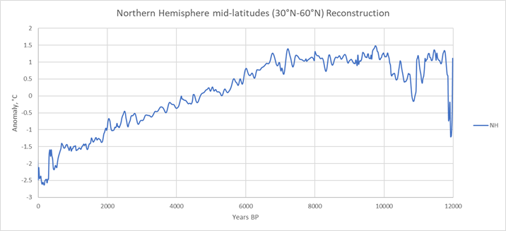
Figure 1A, all proxies that meet the basic criteria (resolution and span)

Figure 1B, excludes KY07-04-01 and OCE326-GGC26
If all proxies are included, as in figure 1A, this reconstruction shows a very flat Holocene Climatic Optimum (HCO) from 10000 BP to 6800 BP and then a steady decline in temperatures to the Little Ice Age (LIA) around 240 years ago (180 BP or about 1770 AD). The range of Holocene temperatures in both reconstructions is 4°C, this is the largest range of any region, including the Arctic. We generally prefer the reconstruction in figure 1B and will discuss the features of this reconstruction here. Since the temperature change in this reconstruction exceeds that seen in the Antarctic and Arctic reconstructions, it calls into question the concept of “Polar Amplification.” We cannot say polar amplification does not exist, but we do not see evidence of it in these proxies. Excluding the two anomalous proxies the coldest portion of the LIA was around 1610 AD.
The 17th and 18th centuries were a time of intense cold weather in Europe, Asia and North America, these centuries were the worst part of the LIA. The early 18th century saw lakes freeze solid in Italy and ice skating took place in Venice. Ships were frozen into ice in New England in 1740. More stories of the severe cold in the Northern Hemisphere in the 18th century can be seen here. The 17th century, if anything, was worse. The 17th century revolutions, droughts, famines, wars and other calamities are detailed in Geoffrey Parker’s book Global Crisis.
In Parker’s book, we see historical records of unusually cold and devastating winters that occurred in Europe and the Middle East in 1620, the United States between 1640 and 1644, China in 1640, Hungary between 1638 and 1641. 1641 remains the coldest year ever in Scandinavia. In the Balkans, in 1654, wine and olive oil froze in jars. In Egypt, in the 1670’s, a country where furs were unknown, was so cold that the citizens started wearing fur coats. Crop yields plunged in Guangxi and Guangdong (Hong Kong area) in southern China due to very cold weather in 1633 and 1634. Icebergs floated down the Thames River in January of 1649 as Charles Stuart was beheaded. In 1698 it was reported, in London, by John Evelyn that the weather was colder than anyone could remember. Harvests failed in Scotland every year between 1688 and 1698 mainly due to cold. And the stories go on and on.
The highest Medieval Warm Period (MWP) peak is at 890 AD. The Medieval Warm Period is very tepid in this reconstruction. Some of the proxies show a bump near the historical MWP and some do not. Below are plots of each set, figure 2 is the set with a visible MWP and figure 3 is the set without.
The proxies with an apparent MWP in figure 2, reach their peaks at different times and they do not line up well, this spreads out the MWP in a reconstruction and dampens the amplitude. The only two that line up are Flarken Lake (Sweden) and D13822 (Portugal). The MWP peak in the MD01-2421 composite from Japan occurs a little later it does in the Newfoundland proxy OCE326-GGC26. MD95-2015 (southwest of Iceland) is a very anomalous proxy with peaks at 1110 AD and 760 AD. In short, in this reconstruction, while it appears the LIA is well defined, the MWP is not. The historical warming from around 760 AD to 1200 AD shows up in these proxies, but not as a single well-defined event.
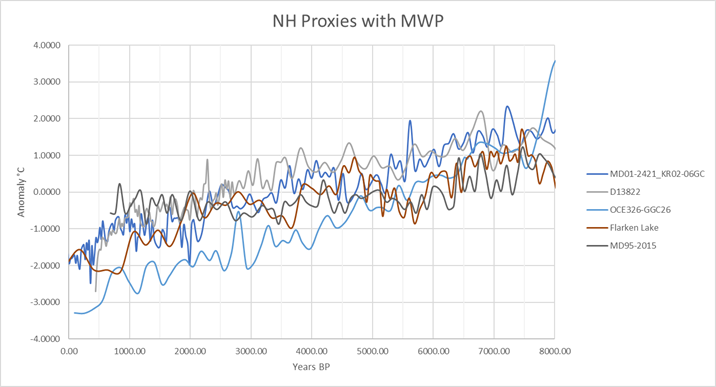
Figure 2
The Northern Hemisphere proxies in figure 3 do not have a noticeable temperature anomaly in the MWP. KY07-04-01 is in the East China Sea, south of Japan. CH07-98-GGC19 is off the US east coast near Washington, DC; it shows a minor bump around 1060 AD to 900 AD. OCE326-GGC30 is near Nova Scotia, Canada; it shows no response at all. The IOW merged dataset is from the Baltic Sea near Sweden and it also shows no MWP response. These proxies run counter to historical records for this time period.
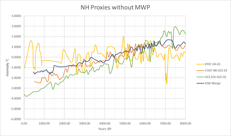
Figure 3
The Roman Warm Period peak is at 90 BC (figures 1A and 1B) and very noticeable in the reconstruction. So, we see the LIA and the Roman Warm Period here, but the MWP not so clearly. This could be because the proxies are erroneous or because the MWP occurred at different times in different areas and was dampened by averaging. The MWP exists, it is a matter of historical record, but it does not show up well in these proxies.
All nine proxy records are shown in figure 4A.

Figure 4A, all proxies

Figure 4B, proxies used
The anomalous records in figure 4A are OCE326-GGC26 (Sachs 2007, near Newfoundland), KY07-04-01 (Kubota et al., 2010, just south of Japan) and Flarken Lake (Seppa et al., 2005, in Sweden). Flarken Lake is probably being affected by meltwater from glaciers that remained in the area long after the last glacial maximum. The retreating ice delayed the Holocene Climatic Optimum in many northern areas (Bender, 2013). We do not think Flarken Lake was a problem and retained the proxy.
OCE326-GGC26
This proxy is just south of Newfoundland and near the Grand Banks. See the location map in figure 5. This proxy record is plotted alongside its neighbor, OCE326-30GGC, in figure 6. Both proxies agree well from 8000 BP to 0 BP, then OCE326-GGC30 flattens out like most of the Northern Hemisphere proxies and OCE326-GGC26 makes a large jump in temperature ending with a 7°C anomaly 11410 BP. This proxy is problematic and was excluded from the reconstruction.
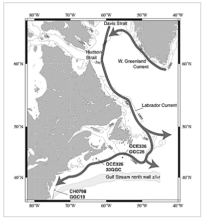
Figure 5 (source: Sachs, 2007)

Figure 6
KY07-04-01
This proxy was also excluded from the reconstruction for being anomalous. The core is from the East China Sea near the southern tip of Japan. See the map in figure 7.
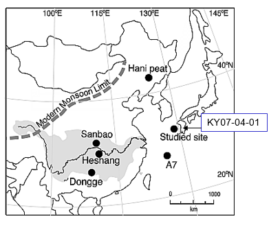
Figure 7 (Source: Kubota, et al., 2010)

Figure 8
The KY07-04-01 proxy is plotted in figure 8. The proxy is very flat from the present day to 10000 BP, with minor fluctuations up and down. This is a Mg/Ca proxy and the core is located near the mouth of the Changjiang (or Yangtze) River. This river is the largest in China, and has its mouth north of Shanghai. The water here is a varying mixture of fresh water from the river and sea water from the East China Sea. The composition of the water varies with monsoon intensity. The river discharge has also varied during the Holocene as inland glaciers melted. Finally, as noted in Kubota, et al. (2010), this temperature proxy does not compare well with other proxies in the area. The other proxies show normal cooling during the Holocene, see the lower portion of figure 9, which is taken from Kubota, et al., 2010. We chose to exclude this proxy from the reconstruction.
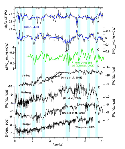
Figure 9 (source: Kubota, et al., 2010)
A map of all the Northern Hemisphere proxy locations can be seen in figure 10. For this region, we have a widespread set of proxies.

Figure 10
The Northern Hemisphere proxies represent a larger range of temperatures and a larger range of temperature anomalies than the other regions. For this reason, proxy drop out at the beginning of the proxy records, about 12000 BP, causes larger than normal temperature fluctuations. This is easily seen in figure 4A between 12000 BP and 10000 BP. Even after excluding KY07-04-01 and OCE326-GGC26, unrealistic fluctuations appeared as proxies ended in the early time and dropped out. To avoid this, we deleted the earliest 3 samples of OCE326-GGC30 and the earliest 20 samples of CH07-98-GGC19. By comparing the right side of figures 4A and 4B you can see what was eliminated.
Proxy drop out at both ends of the reconstructions is a problem. We are using anomalies from the mean for these reconstructions which helps, since the anomalies tend to have similar ranges. But, in the case of the Northern Hemisphere, even the anomalies have widely different values and depending upon the order in which they drop out, they can cause strange spikes at the beginning and the end of each reconstruction. The earliest few values and the last few values for the Northern Hemisphere proxies are shown in figure 11 as an example.
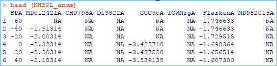

Figure 11
At 0 BP (1950 AD, the upper panel) we have no values for four of the proxies, “NA” means no value. The three remaining proxies have values of -1.698, -3.422, and -2.323, that average to -2.481. At -20 BP (1970) we only have two values as GGC30A has dropped out, so the average is a very different -1.86. Compare this to the situation at very early time where the MD012421 proxy is about -5.5 and the GGC30 proxy is 1.84 and you can see the problem with drop out in the Northern Hemisphere. This problem is much less pronounced in the other regions which show less variability. We only trimmed excessive values like this in the Northern Hemisphere.
Arctic reconstruction
The Arctic reconstruction is shown in figure 11. The R code and input and output datasets can be downloaded here.
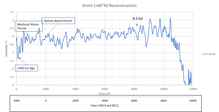
Figure 11
The lowest point in the LIA in this reconstruction, occurs at 1850 AD. There is no well-defined Medieval Warm Period, but there are peaks at 850 AD and 1070 AD. The Roman Warm Period is seen from 270 BC to 50 BC. Figure 12 plots the nine component proxies.
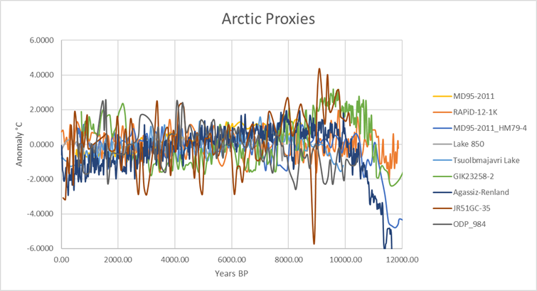
Figure 12
A map showing the proxy locations is presented in figure 13. The proxies are all in the north Atlantic area, but widespread.

Figure 13
Only JR51GC-35 and GIK23258-2 look a little anomalous, but not severely so. GIK23258-2 (Sarnthein, et al., 2003) is the most northerly proxy with a latitude of 75°N. This may explain the slightly anomalous warm anomalies at about 9000 BP and between 2500 BP and 1000 BP. The Iceland proxy JR51GC-35 is quite spiky. The location of the JR51GC-35 is shown in figure 14. It is in an area where multiple currents can influence the temperature quite dramatically, which probably explains the spiky nature of the curve.

Figure 14
Conclusions
These regions have the most data and are probably well represented by the proxies. The Northern Hemisphere mid-latitude reconstruction is quite different from the other regions. Most of the regions show a Holocene temperature variability of ±1°C whereas the Northern hemisphere reconstruction shows a temperature variability of ±4°C.
Considering the abundant historical evidence from the Northern Hemisphere for the Medieval Warm Period, it is odd that this climatic event does not show up well in the Northern Hemisphere reconstruction. It is possible that this warming event took place in different areas at different times and this smeared and dampened the record. The variation in the Northern Hemisphere proxies suggests that the climatic history of the Northern Hemisphere was very complex during the Holocene, relative to the other regions.
We see no evidence of polar amplification in these reconstructions. The Northern Hemisphere mid-latitudes shows a larger range of temperatures than either the Arctic or the Antarctic.
The Northern Hemisphere reconstruction illustrates the problem with proxy selection and with temperature proxies in general. Proxies are not thermometers, they do not measure temperature directly. They react to temperature in the present day in a certain way and we assume they react in the same way in the distant past. How accurate are the temperature estimates? Further, we assume that burial and time have had no effect, or a predictable effect on the quantities measured. We assume that we have measured the age and depth or height of each sample accurately. Finally, we assume that each proxy represents the surface temperature of a very large area with no local distortions. So, how do we choose which proxies to include and which to reject? Our basic requirements of a span of 9000 BP to 500 BP and a resolution better than 130 years are reasonable. Was it reasonable to reject KY07-04-01 and OCE326-GGC26? Perhaps, but it is hard to tell, the decision was mostly subjective.
In the next post, we will present a global reconstruction. We will also discuss the various sources of error in the proxies.
The R code and input and output datasets for the Arctic reconstruction can be downloaded here.
I am very grateful to Javier who has read this post and made many very helpful suggestions. Any errors are the author’s alone.
At the rate you’re going, I won’t have anything left to do when I retire… 😉
Great work, as always, Andy!
…oh, we’ll come up with something
Thanks Andy!
Thanks for these posts, A.M. They are very informative.
When the demands made by advocates of “climate change” converge far more to socialistic government policies and attack human prosperity than they can possibly improve the environment, it should be clear that no amount of solid research will change the desired end goal.
Now if only we can figure out a cause. . .
Here’s a thought: There is no one cause over any one span of time. Rather, there might be an apparent cumulative effect of MULTIPLE causes which are all inter-meshed in ways that no current theory or model has yet clarified.
+1
Robert,
You are very probably correct.
There are many factors that can – or do – influence temperature – and thus, over decades and centuries, and more – climate.
We probably know of many or most of them.
We may not be able to quantify them, and their interactions may bemuse us still.
So – like the weather in England, a prediction of four hours may very well be good.
A prediction of twenty-four hours needs to be comparted with other similar predictions [and not implicitly trusted]; –
and a seven/thirty/ninety day prediction should – if you must print out – use soft paper and let it be relegated to bathroom detail.
And yet we have ‘scientists trying to call weather and climate ninety years hence.
It reminds me of the (apocryphal?) comment on a Civil Service memo, purportedly over a hundred years ago: –
‘Round Objects.’
Another comment, immediately below, was :
“Who is Round? And to what, specifically, does he object?”
Auto
I will possibly move to Hungary If the Election allows a horrifically backward looking party into power . . .
Just agreed with my lodgers.
Are proxy sources/data selected only at coastal locations? Are we then to assume that the land measurements were taken for these regions not covered by proxy data (doubtful as no temperature measuring devices existed)? Why are there no proxy sources from Central Asia or North America?
Yup X 100!
Marine proxies are nearly meaningless as they show a lack of variance that is very deceptive. I visited the area North of San Francisco a couple of years back. Inland 10 miles it was about 15-20F warmer most days but much more variable while at the coast it was cloudy and 50-55F every single day. Looking at the weather averages for the area before I went I saw that the coast temps were around that most of the year.
The Arctic reconstruction, Figure 11, is at odds with the Viking settlement of Greenland. link The Vikings had a few centuries, starting with the MWP, when the Greenland climate was reliable enough to support their civilization.
5th paragraph down, “were furs…” should be changed to “where furs…”
Andy May, thank you for your essay, and its two predecessors.
Except for the “Year without a Summer,” the most extreme events reported in the historical record are Winter events. Plants aren’t growing in the Winter, so one shouldn’t expect tree rings to capture the Winter events, and frozen rivers and streams aren’t moving sediment. Perhaps the uncertain MWP is a result of averages not capturing the low Winter temperatures.
Trees can only tell you when the conditions are just right for them to grow….
Andy May,
Thank you (!) for your deliberative and thoughtful analyses of these various temperature proxy reconstructions.
Andy,
Your work is bringing up interesting issues to discuss, and I would like to talk a little bit about it in relation to well known features of relatively recent climate variations that we have all come to know about.
The Little Ice Age is well featured in your work as a global phenomenon, and consistent with global glacier evidence and historical accounts. Only a person (I wouldn’t call it scientist) that hasn’t bothered reading the relevant information would question that the LIA represents the coldest global multi-centennial period in the entire Holocene.
Now I would like to discuss about the Roman, Medieval, and Modern warm periods.
The Roman warm period represents the longest warm climatically uneventful period of the entire Holocene, and this is a fact little acknowledged. No wonder that it coincided with the longest multi-continent empire in history. While the Holocene climatic optimum was warmer and more humid, it was periodically interrupted by cooling from the 1000 and 2400 year solar cycles as it has been registered by the Bond series of increased ice drift events. The Roman warm period however appears as a long gap in the Bond series between around 2600-1400 BP (650 BC – 550 AD), the longest such gap. This explains why glaciers retreated so much at the time, as they had a much longer time to melt. The likely reason is that both the 1500 year cycle and the 2400 year cycle skipped that period while the 1000 year cycle was not active at the time, according to solar activity proxies.
As the proxies you and Marcott et al., 2013 are using are mostly marine proxies, they also had ample time to reflect the Roman Warm period. It is very important to consider the nature of the proxies used in a reconstruction and how they respond to changes.
However the Medieval warm period was very different in nature. It was quite brief. Temperatures were increasing around 900 AD and reached a peak between 1000-1100 AD, and by 1250 AD it was mostly over. Some marine records might have not properly recorded it for lack of time. It is properly registered in Northern Hemisphere reconstructions that rely more on terrestrial proxies, like Mohberg 2005, Wanner 2008, or Ljungqvist 2010.
Which brings us to the last question. Most skeptics rely heavily on GISP2 to get their idea of how the climate was in the past, and I have defended here that it is not possible to determine with the available information if the Medieval warm period was warmer or not than the present global warming. Apparently this goes against the skeptic bible, but since I don’t subscribe to religious beliefs easily, I’ll rather wait until there is convincing evidence.
I don’t understand the dating techniques all that well. One possibility for the lack of alignment between warm/cold periods could simply be dating problems. If this was the case then realignment based on the data might give a slightly different answer.
Most of the dates are radiometric dates. I’ve more on this in part 4. You are correct that dating problems are one of the big issues with reconstructions of this type.
High surface level pressure (and temperature) dancing around the northern hemisphere mid latitudes during the MWP isn’t terribly surprising, given the way it dances around today. Ridiculously resilient ridges and terribly tenacious troughs are the norm.
I jumped into this article (missing the first two) and could not make out what kind of proxies where being considered – there are all sorts of proxies and each has its problems. Finally, back tracking to the original paper I came across the text below and now I can understand this article. Including this paragraph from the earlier paper in case anyone else has missed reading it…I advise you go back and start at the first article “A Holocene Temperature Reconstruction Part 1: the Antarctic By Andy May” or this article will make little sense. There is a spreadsheet you can load that has information on all the proxies in the first article.
Excerpt: “It is very logical to investigate long term climate changes using ocean temperature proxies from foraminifera shells and fossils (“forams”), planktonic and algal material. Traditionally the magnesium and calcite (Mg/Ca) percentages or δ18O ratios in planktonic foraminifera have been used to deduce ancient sea surface temperatures. On land, ice core δ18O records and pollen are used to estimate ancient air temperatures. More recently we have seen more use of haptophyte algal alkenones, especially the U37K’ (also written as UK’37) index to get ancient sea surface temperatures, see the link here. TEX86 records from marine plankton have also been used recently to obtain sea surface temperatures and are among Marcott’s proxies, see here for a discussion. The original reference for the TEX86 sea surface temperature proxy is Schouten, et al. (2002) here. A complete list of the proxies used by Marcott, plus one I added from Rosenthal, et al. (2013) and references and links to the original papers can be downloaded here. I did not use all Marcott’s proxies in my reconstructions, those that I did use are noted in the spreadsheet.”
Now with the proxies understood, the fact that they are all over the place on temperature is understandable. I believe these kind of reconstructions are very coarse and cannot reflect temperature variations with any degree of accuracy. There are just too many conditions that can affect most or all of them. The fact that so many of them actually agree in a general trend line surprises me. Yes, they can show a very general correlation to temperature, but getting it down to +/- 2C is likely pushing it. I note there are no error-of-margin on the plots of the proxies, so it’s hard to tell just how much they actually overlap or disagree (except in trend).
Very Interesting article, thanks.
There will be more on error in part 4 or you can read Marcott et al.’s supplementary material which has a very thorough discussion of most of the error/uncertainty issues. The other issues I cover in the next part, which should be up tomorrow.
From the post, “..The proxies with an apparent MWP in figure 2, reach their peaks at different times and they do not line up well…”,This is likely the “wave” pattern which had caught my eye a few years back as I was studying the different regional graphs depicting temp changes in regions of the NH. The JG/U tree ring study was the trigger for some odd reason. As I was interpreting that graph in my fashion, of a sudden I experienced a “slideshow” of the different regional graphs of which I had viewed. As I viewed this I could see/understand that there was a wave pattern where the warming would move regionally over time. I have always meant to take another more thorough look at that to see if I could flesh out more detail from the thoughts which automatically arose within me at the time.
Thanks for that comment. I can’t verify this, but it looks like the MWP occurs at different times in different places. It looks strong when viewing one proxy, but as you add them it smears and dampens.
Could the variance be equated to a cup of coffee [Or any liquid… :-)] in warm vs. cold state? The atmosphere above a hot cup of coffee, and indeed the liquid itself will be much more heterogenous/variable and express more complex form than the same cup in frozen form… ie. the colder the temperature the less variability and perhaps hence the more stable the proxy readings?? I was envisaging the swirling vapour and liquid in a hot cup vs. what must be more static form in a cooler cup… What do you think, could that contribute to the disparity you see between LIA and MWP readings?
See Wyatt and Curry’s 2014 Stadium Wave paper, available at her blog Climate Etc.
I remember when their paper came out. I came across this idea in August of 2012 after seeing the JG/U paper which came out in July of that year. I made about 3 or 4 comments to that effect at the time here at WUWT, but as no one responded to my comments I just filed the thought away for a later day.
Also, “…The Northern Hemisphere proxies in figure 3 do not have a noticeable temperature anomaly in the MWP. …”, the effects of ocean moderation on temp records? Note that the CET does not line up with inland/continental NH temp records, and that makes perfect sense to me as the Atlantic currents are the moderator of CET temps. Wouldn’t the same hold true for many if not all coastal locations? The data reflects the state of the offshore waters.
This ” data reflects the state of the offshore waters” would have been better stated as ” the data reflects the influences of the Atlantic on the CET”.
Today or tomorrow will be sea ice passover day. Waning Arctic sea ice extent will become smaller than waxing Antarctic today or tomorrow, according to NOAA.
Or crossover. Less religious connotation.
Merely the lower node of a sinusoidal curve as the slope passes from negative to positive as it passes through horizontal.
What is the temperature anomaly in figure 1 relative to?
The average temperature from 9000 BP to 500 BP.
Amusing that Mann, et al, imagine the Medieval WP was only a North Atlantic regional event, yet it shows up everywhere except in that area in these proxies.
Thanks!
Polar amplification: I suspect that real changes, particularly in Antarctica, are muted because at generally very cold temperatures, , swings of a few degrees are not going to be significantly reflected. That is to say the sensitivity attenuated in the cold end. What’s the difference say between – 50C and – 53C. This is intuitive I admit imagining myself out in such conditions (Winnipeg recorded – 50C New Years day 1968 – I had returned with wife and kids from N Nigeria where it was ~+40C into a cool fall in 1967).
My comments # 2522543 and 2522648 have disappeared without trace. I don’t know what is going on.
The first of those two has appeared above, but not the second. Yet.
“Considering the abundant historical evidence from the Northern Hemisphere for the Medieval Warm Period, it is odd that this climatic event does not show up well in the Northern Hemisphere reconstruction. It is possible that this warming event took place in different areas at different times..”
Is this not just another way of saying that there was NO Medieval Warm Period? i.e. there was no globally significant warming during that time that warrants the name. Rather different regions had the usual fluctuations in temperature all of which is consistent with a noisy system.
Just throwing this out there, but isn’t the comet impact theory supposed to have happened between 11000 and 12000 BC? Perhaps an influence on the outliers?
Thank you for the list of uncertainties. I may be a Simple Red Neck, but I believe that is what a REAL scientist does.
In another application of earth sciences that consumed much career time, I would have given a quick glance to a graph like your all proxies Fig 4A, then thrown it in the bin.
Andy, I do appreciate the work you and the other authors have put into this. I comprehend the value of proxies that can be trusted.
But realistically, have we lost sight of the point at which we say “The signal, if any, is lost in the noise”?
Maybe others feel as I do, that when the data needs such torture to confess, it is unlikely to produce a result one can take to the bank.
Geoff
Andy,
Why are there only about 60 proxies worldwide? Are these all for trees? I saw one for mg/Ca. I’d like to know more perspective on the number and type of proxies overall.
Thanks,
John
“Considering the abundant historical evidence from the Northern Hemisphere for the Medieval Warm Period, it is odd that this climatic event does not show up well in the Northern Hemisphere reconstruction. It is possible that this warming event took place in different areas at different times.”
Given a dominance of La Nina and positive North Atlantic Oscillation states, the regional response would be very varied. Higher definition individual proxy charts just between 500 and 1500 AD would aid the analysis of the MWP. Esper et al shows the MWP warmest for Europe in the late 8th century.
I don’t think there is anybody checking the messages that don’t get posted. This is ridiculous. Four attempts in the last 24 hours. I will try posting it in chunks.
Andy,
Your work is bringing up interesting issues to discuss, and I would like to talk a little bit about it in relation to well known features of relatively recent climate variations that we have all come to know about.
The Little Ice Age is well featured in your work as a global phenomenon, and consistent with global glacier evidence and historical accounts. Only a person (I wouldn’t call it scientist) that hasn’t bothered reading the relevant information would question that the LIA represents the coldest global multi-centennial period in the entire Holocene.
Now I would like to discuss about the Roman, Medieval, and Modern warm periods.
The Roman warm period represents the longest warm climatically uneventful period of the entire Holocene, and this is a fact little acknowledged. No wonder that it coincided with the longest multi-continent empire in history. While the Holocene climatic optimum was warmer and more humid, it was periodically interrupted by cooling from the 1000 and 2400 year solar cycles as it has been registered by the Bond series of increased ice drift events. The Roman warm period however appears as a long gap in the Bond series between around 2600-1400 BP (650 BC – 550 AD), the longest such gap. This explains why glaciers retreated so much at the time, as they had a much longer time to melt. The likely reason is that both the 1500 year cycle and the 2400 year cycle skipped that period while the 1000 year cycle was not active at the time, according to solar activity proxies.
The Roman warm period represents the longest warm climatically uneventful period of the entire Holocene, and this is a fact little acknowledged. No wonder that it coincided with the longest multi-continent empire in history.
The Roman warm period is the longest period without cold events in the entire Holocene, and this is a fact little acknowledged. Perhaps it relates to coinciding with the longest multi-continent empire in history.
While the Holocene climatic optimum was warmer and more humid, it was periodically interrupted by cooling from the 1000 and 2400 year solar cycles as it has been registered by the Bond series of increased ice drift events. The Roman warm period however appears as a long gap in the Bond series between around 2600-1400 BP (650 BC – 550 AD), the longest such gap. This explains why glaciers retreated so much at the time, as they had a much longer time to melt. The likely reason is that both the 1500 year cycle and the 2400 year cycle skipped that period while the 1000 year cycle was not active at the time, according to solar activity proxies.
As the proxies you and Marcott et al., 2013 are using are mostly marine proxies, they also had ample time to reflect the Roman Warm period. It is very important to consider the nature of the proxies used in a reconstruction and how they respond to changes.
However the Medieval warm period was very different in nature. It was quite brief. Temperatures were increasing around 900 AD and reached a peak between 1000-1100 AD, and by 1250 AD it was mostly over. Some marine records might have not properly recorded it for lack of time. It is properly registered in Northern Hemisphere reconstructions that rely more on terrestrial proxies, like Mohberg 2005, Wanner 2008, or Ljungqvist 2010.
Which brings us to the last question. Most skeptics rely heavily on GISP2 to get their idea of how the climate was in the past, and I have defended here that it is not possible to determine with the available information if the Medieval warm period was warmer or not than the present global warming. Apparently this goes against the skeptic bible, but since I don’t subscribe to religious beliefs easily, I’ll rather wait until there is convincing evidence.
A two-phrase paragraph just refused getting posted. I had to rewrite it in a different manner. Most curious.
Javier,
I feel your frustration. But be aware that it is the Russians hacking this site. (:-)).
Yeah! It seems they finished early hacking Theresa May’s elections in Britain, or maybe some of them got confused because Andy has the same last name XD
Javier, have a quick thought for consideration. Since H20 vapour is a much more powerful greenhouse gas than CO2. Wouldn’t we be considering the change in temperatures as more of a change in H20 vapour. Trees being a central part in the hydrological cycle. Beavers also change the hydrological cycle likely more than humans, perhaps the change in the number of trees and eradication in beavers caused a major change in the GHG’s and therefore surface temperatures in Europe and other places?