By Andy May
In the last post (see here) we introduced a new Holocene temperature reconstruction for Antarctica using some of the Marcott, et al. (2013) proxies. In this post, we will present two more reconstructions, one for the Southern Hemisphere mid-latitudes (60°S to 30°S) and another for the tropics (30°S to 30°N). The next post will present the Northern Hemisphere mid-latitudes (30°N to 60°N) and the Arctic (60°N to the North Pole). As we did for the Antarctic, we will examine each proxy and reject any that have an average time step greater than 130 years or if it does not cover at least part of the Little Ice Age (LIA) and the Holocene Climatic Optimum (HCO). We are looking for coverage from 9000 BP to 500 BP or very close to these values. Only simple statistical techniques that are easy to explain will be used.
Southern Hemisphere mid-latitudes
Our reconstruction for this region is shown in figure 1. The R code and the input and output datasets for the Southern Hemisphere mid-latitudes can be downloaded here.
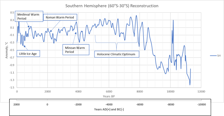
Figure 1
This reconstruction has a more defined HCO than we saw in the Antarctic and it is placed between 8000 BP and 5000 BP. The HCO occurs at different times in different places as discussed by Renssen, et al. (2012). Following this, the temperature generally drops to a low in the LIA. In this reconstruction, we see two LIA lows, one at 1690 AD and one at 1550 AD. The Medieval Warm Period (peak 1030 AD) and the Roman Warm Period (peak 90 BC) are very distinct in this reconstruction. The Minoan Warm Period (peak 1890 BC) can also be seen.
There are only four proxies in this reconstruction, three in New Zealand and one off the coast of Chile. The locations are shown in figure 2.
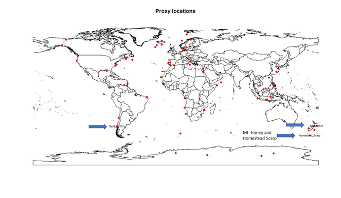
Figure 2
Two of the proxies have been combined into one record, the three proxies used are plotted in figure 3.
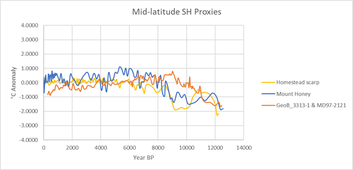
Figure 3
Three proxies were rejected due to large sample intervals, TN057-17 (Nielsen, et al., 2004) was rejected because it was very anomalous. See the plot in figure 4.
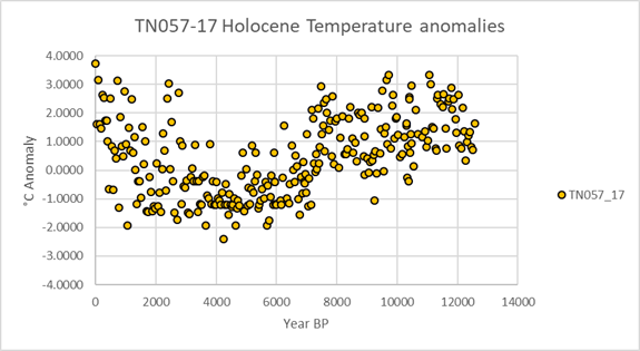
Figure 4
TN057-17 is a sea surface temperature proxy located in the Southern Ocean, right on the Antarctic Polar Front (APF), see Figure 5. The APF has a very abrupt sea surface temperature change. It is the southern limit of synchrony with the Northern Hemisphere climate system. This location, currently, has sea ice cover about two weeks per year (Nielsen, et al., 2004) but the time of ice cover has changed a lot during the Holocene and this has probably had a dramatic effect on the proxy. The maximum sea ice cover was 4300 BP, which is also the time of the lowest TN057-17 temperature.

Figure 5, source (Nielsen, et al., 2004)
Sea ice presence (SIP) at the TN057-17 location is shown in figure 6.
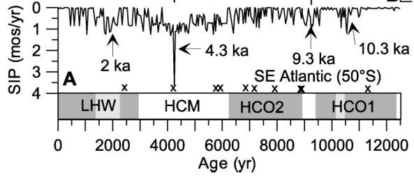
Figure 6, Sea ice presence (SIP) at TN057-17 (Source: Nielsen, et al., 2004)
There is a risk that the TN057-17 proxy has been affected by local conditions that are only vaguely connected to climate change and for this reason the proxy was rejected.
The Chilean GeoB 3313-1 proxy (Lamy et al., 2002) only went back to 7000 BP and for this reason would be rejected on its own. But, the New Zealand proxy MD97-2121 (Pahnke and Sachs, et al., 2006) has nearly the same latitude and is continuous from 12464 BP to 3316 BP. So, these two proxies were merged by adjusting them to the mean of the overlapping interval 6900 BP to 4000 BP. See figure 7.
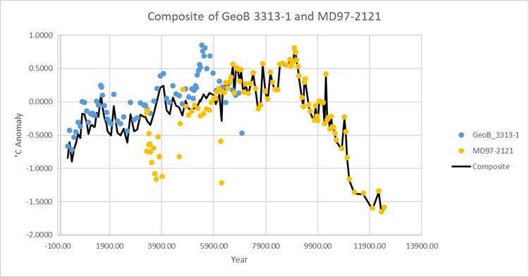
Figure 7
The logic in combining these two proxies is it gives us one more proxy in a region that has few available and, at least part of this composite is outside the New Zealand area. The most recent portion of MD97-2121 (4000 BP to 3300 BP) was not used in the composite as it looked suspicious. Pahnke and Sacks (2006) report that the MD97-2121 core top (the most recent sediments in the core) may be problematic due to lack of recent sediments at the cored location. In any case, a 3000-year-old core top, presumably close to the sea floor, has probably been churned quite a bit and should be greeted with suspicion. Older than 4000 BP, the results are consistent with GeoB-3313-1.
Tropics
The reconstruction for the tropics (30°S to 30°N) is shown in figure 8. The ODP-658C proxy is problematic, so we present a reconstruction including it in figure 8A and one without it in figure 8B. The R code and the input and output datasets for the tropics can be downloaded here.
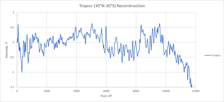
Figure 8A, with the ODP-658C proxy

Figure 8B, without the ODP-658C proxy
There is a very distinct LIA at 1630 AD. The two peaks around the classical MWP are 1090AD and 930 AD. The Roman Warm Period (90 BC) and the Minoan Warm Period are apparent. In this reconstruction, the HCO is from 9600 BP to 7700 BP.
There are eight usable proxies in the tropics using our criteria, they are plotted in figure 9.

Figure 9
The location of the proxies is shown in figure 10, there are quite a few in Indonesia so we did not put arrows on the figure for each one. One of the Indonesian proxies, Ros_BJ813GGC, is not a Marcott et al. (2013) proxy. It is from Rosenthal, et al. 2013.

Figure 10
The rejected proxies, except for ODP-658C, were all because of resolution or because they did not cover the period from the Holocene Climatic Optimum to the Little Ice Age. ODP-658C (deMenocal et al., 2000) is the brown line in figure 9. It is located off West Africa, the northern most arrow off West Africa in figure 10. The proxy is plotted in figure 11. This proxy was left out of the final reconstruction, but figure 8A shows a reconstruction that includes it.

Figure 11
The sharp break in the proxy at 5700 BP appears to be a data problem until we consider that this is the end of the African humid period when the Sahara turned into a desert due to the abrupt movement of the Intertropical Convergence Zone or “ITCZ” (deMenocal et al. 2000 and Javier, 2017). Figure 12 shows the worldwide change that took place around 5700 BP, it is from Javier’s essay here. This change in the location of the climatic equator (ITCZ) is often called the Mid-Holocene Transition when the world goes from the Holocene Climatic Optimum (HCO) period to the Neoglacial period. This data suggests that the Mid-Holocene Transition, in this area, occurred in less than 120 years between 5808 BP and 5683 BP using the dates given by deMenocal, et al. This is how long it took for sea surface temperatures at the ODP-658C location to increase over 2°C. The core location is shown in figure 12 with a red star. Around 5700 BP the ITCZ migrated from north of this location to south of it.
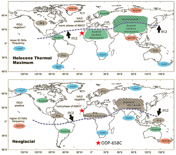
Figure 12 (Source: Javier, here)
The proxy temperature record labeled 17940 (Pelejero, et al., 1999) from the South China Sea could also be considered slightly anomalous since in the Neoglacial period it trends warmer, rather than cooler. It also shows no Holocene Climatic Optimum. The proxy is displayed below in figure 13.

Figure 13
The South China Sea is a very large marginal basin in the western Pacific. It is bounded by broad shallow shelves in the northwest and southwest that emerge during periods of low sea level. Sea level was low enough during the early Holocene for these shelves to be emergent. The position of the shelves can be seen by following the 100-meter isobath (water depth) contour in the map in figure 14. In addition, core 17940 is only 400 km from the mouth of the Pearl River, the second largest river in China. Due to the large sediment discharge from the river the location has a very high sedimentation rate, further it was larger in the past as the glaciers retreated to their present position and sea level was lower. We kept the proxy in the reconstruction, but recognize that it is sensitive to the changes in sea level experienced during the Holocene and to changes in the discharge rate from the Pearl River. The sea surface temperatures of the other cores in the South China Sea are similar.

Figure 14 (Source: Pelejero, et al. 1999)
In the next post, we will discuss the Northern Hemisphere Holocene proxies and the Arctic proxies. The supplementary materials for the tropics reconstruction can be downloaded here.
Conclusions
The Southern Hemisphere mid-latitude reconstruction is built from very little data. The data is mostly in the New Zealand area and cannot be considered representative of the whole region. But, we work with what we have.
The tropics reconstruction is built from widely dispersed proxies that sample all major ocean basins. It is probably representative of the region. The reconstruction without the anomalous ODP-658C proxy is probably the best to use. The Mid-Holocene Transition is a real event, but probably had no global temperature effect. It is merely a shift in the climatic equator or the Intertropical Convergence Zone or “ITCZ.” The ODP-658C location warmed dramatically 5700 BP, but presumably another location, that is not sampled, cooled as dramatically. Including the warming at the ODP-658C site, without the cooling elsewhere distorts the regional and global picture. Therefore, we excluded the proxy.
I am very grateful to Javier who has read this post and made many very helpful suggestions. Any errors are the author’s alone.
Today is D Day plus 73 years – this article is about the weather forecast:
https://www.vencoreweather.com/blog/2017/6/5/1030-am-the-most-important-weather-forecast-of-all-time-d-day-june-6-1944
I suggest that any shift of the ITCZ latitudinally is a negative system response to any change in the system that seeks to take the system away from the thermal equilibrium imposed by conduction and convection acting via atmospheric mass held within a gravitational field.
Thus I agree that such a shift does not represent a change in the average global surface temperature being instead an adjustment to new internal system condition.
The response to anthropogenic influences would be similar but infinitesimal.
We should not worry when they reject a proxy because it is anomalous.
Well if it’s anomalous to the point where we can reject it, we can also be sure that Mother Gaia ignored it as well, because it was anomalous, so she didn’t alter the local climate just because some stuff was anomalous.
It’s a good system; Mother Gaia can ignore the laws of physics any time she wants to, and just make the climate what she thinks it should be.
So we should ignore it too.
G
If these Southern hemisphere proxies are anywhere near right, so much for the assertion that the LIA was regional, and Mann et al is right.
Tom, it looks like the Little Ice Age is labelled on figures 1 and 8B, occurring between the Roman and Modern Warm Periods. However, I take note of Prof. Easterbrooks comments about proxies, especially as some of the data, as depicted, shows a lot of noise in different sectors. However, the work by Andy does seem to be showing world-wide climate variations that, in more recent times including the Little Ice Age, correlate fairly well with solar cycles as measured by sunspot activity.
The evidence for the global extent of the Little Ice Age is extensive and robust. There is excellent correlation with sun spots, solar irradiance, cosmic radiation (as shown by 10Be and 14C), ice core isotopes, and historic measured temperatures. All of these are discussed in the new Elsevier volume “Evidence-based Cllkimate Science.”
You don’t need to go to temperatures to know that the LIA affected almost the entire world. All over the planet, most glaciers display their highest extent during the Holocene at the LIA. It is impossible to adjust the moraines that prove it.
I have no doubt that the Little Ice Age was real but I’m afraid I roll my eyes a fair bit when I see so many proxies derived from coastal locations. Marine environments are pretty lousy places to look for variance as far as I’m concerned. The next time I see a temp reconstruction from the Antarctic peninsula standing in for a climatic history of the continent of Antarctica I think I’m going to burst a blood vessel. This is the kind of trash science I expect to see from the Warmists.
The best Pleistocene climate record in my opinion is the LR04 stack [Lisiecki and Raymo, 2005] that spans 5.3 Myr and is an average of 57 globally distributed benthic dO records. When you want to know how the global climate evolved you don’t want too much variance, and the benthic records will give you the bottom line.
Thanks Javier! I’ll look for it.
I think the distribution is more important than the numbers. One look at Mann’s choices for proxies shows just how royally somebody with nefarious intentions can screw up a an investigative process. Of course the fact that his “errors” were made obvious to him ,after which he used them again, and his climate science science compadres didn’t call him on it also shows that a conspiracy of bogus science was afoot. Goebbels would be proud of these fraudsters and their big lie.
Is the sampling of proxies sufficient to reconstruct a global estimate?
Pretend that they were thermometers.
If a global average of thermometers doesn’t make sense then a global average of thermometer proxies makes less sense.
There’s an extensive and well known review paper by Dr. (Willie) Wei Hock Soon, and Dr Sallie Baliunas, in which they reviewed dozens and dozens of papers from all around the globe, and their review shows that the MWP and the LIA were indeed global climate phenomena.
YOU are confusing the MWP and the LIA with Michael Mann’s Hockey stick paper.
The ORIGINAL publication of Mann’s (in)famous hockey stick, graph is CLEARLY LABELLED as NORTHERN HEMISPHERE. Check the original IPCC documents.
Hockey sticktion was local ( The Yamal Effect), as Mann asserted.
LIA and MWP were both global.
G
Anyone using the Marcott et al (2013) data should read the critiques by Willis and by me shortly after it was published. (They can be found in the WUWT archives). This was a badly flawed paper–that doesn’t mean that some of the data might not be useful, but caution is advised.
This article refers only to ‘proxy’ data, but doesn’t say anything about what the proxies were. There are big differences in the validity of proxies, so that would have been good to know as you read this paper. You can dig it out of the Marcott et al. paper, but that’s tedious.
Don,
Steve McIntyre at Climate Audit also critiqued Marcott et al (2013) in great detail.
Yes–I should have mentioned that.
Dr. Easterbrook, there is a link in part 1 to a very detailed bibliography for all of the proxies, plus part 1 discusses their validity. I was very selective in what proxies I used. No proxies are perfect and none (including ice core proxies) read actual temperatures. However, they are the best we can do. I share your concerns about Marcott’s analysis methods, that is why I did that part over. He used 73 proxies, of those I used 28. I added one he did not use from Rosenthal, 2013. Here is the detailed list of proxies and references as a spreadsheet. It also indicates those I used or rejected and why: https://andymaypetrophysicist.files.wordpress.com/2017/06/reconstruction_references.xlsx
Thanks, Andy.
You need to test the sensitivity of your reconstruction to selection criteria. That will give you part of your structural uncertainty.
Now they are going to have to rename the Medieval and Roman Warm Periods to the Medieval and Roman Not-so Warm Periods.
Mann was right… the Vikings living in Greenland was a myth. Good work.
It isn’t Marcott et al. data. They just selected the proxies and did the reconstruction. It is other researchers’ data and there is nothing intrinsically wrong with it. Some proxies are more useful than others for certain purposes. All display specific conditions at a certain location.
The very first rule of process control theory is : If you want to control the value of some variable of the system, (say the Temperature of a turkey in an oven), you should MEASURE the value of THE VARIABLE YOU WANT TO CONTROL, and compare that to the desired set point value, as a feedback to those system forcing functions that can influence the value of that variable (like an oven heater for example.)
The process of presuming a cause and effect relationship between a system variable and some proxy for that variable, and applying forcings based on that proxy, is known (in the trade) as FEED FORWARD.
It allows you guess how much power to apply to cook your turkey, and apply that immediately to get there quicker.
It also allows you in most cases to create a disaster, when your proxy turns out to be not very well related to the actual variable you thought you could control. That’s how chemical plants blow up unexpectedly.
It so happens that I just rejected (for a design I am working on) a boost switching voltage regulator, that uses multiple feed forward controls, plus minimal FEED BACK CONTROLS.
And yes, it had a mind of its own and did things that are not described on the data sheet, making it totally useless for what I was doing. A lot of the stuff that is designed in Silicon Valley and other hi tech valleys, is just too damn smart for its own good. The designers simply didn’t think about all of the ” What if’s ? ”
So color me blah on proxies.
G
Andy’s work is important on many accounts. One of them that should be obvious by now, is that by using the same data as Marcott et al. (2013), and rejecting proxies only on objective grounds as lack of resolution or known biases, he is getting an answer that dispels some of the myths that Marcott et al. (2013) spread. There is no better way of refuting bad science that using the same evidence and showing that the conclusions are not warranted. This work should have been done by the scientific community, but they see no personal gain in confronting the alarmist mountebanks. I once commented on Steve McIntyre blog that this should be done, but not sure he even read it. I am glad Andy is doing it, and I just hope we can see more works like his published in scientific journals.
The Marcott paper as published in Science in 2013 comprises clear academic misconduct. This is provable by comparison to the Ph.D thesis version. The forensics was provided at the time at Curry’s Climate Etc. blog by guest post ‘Playing Hockey–Blowing the Whistle’. The evidence was presented to Marsha McNutt, then senior Science editor. Receipt was acknowledged but nothing was done.
One of several clear cases of academic misconduct exposed by climate essays in ebook Blowing Smoke. Others include west Australia SLR, Milne Bay corals, Whiskey Creek oyster hatchery, northern spread of NH pests, and Catalina Highway plant progression.
Rud, please submit your “findings” to a reputable scientific journal. Then maybe someone would take them seriously.
All published. Read and judge the evidence for yourself. The ‘reputable journals’ who published this proven dreck include Science, Nature Geoscience, and Nature Climate Change.
The journals you happen to be railing against have (in terms you will understand) jurisdiction. Blogs, and self-published ebooks don’t set precedents (another term you should understand.) So, when you decide to take your case, petition or appeal (more terms for you) to the journals which comprise the court of science (see how clear I can make it for a lawyer/) don’t belly-ache about what is or is not accepted in science. You have to abide by the rules of the game if you want to play.
You mean like Nature? Karl et al self admitted significance of 0.1?
Can somebody explain to me how the great majority of news outlets and “scientific” journals all seem to have such an extreme bias in favour of the AGW message? I’m not a conspiracy theorist by a long shot but this bias is very obvious. I clearly see the influence of politics in the background but the fact that there seem to be almost no defenders of scientific process or even basic truth or ethics is stunning to me. It ranks up there with rank indifference to National Debt accumulation. The enviro-Left seems to have achieved virtually an absolute lock on the media. How is this possible?
John Harmsworth
The hippies and other well off establishment kids of the 1960s are now in control of all our institutions. I’m their age but not one of them.
They thought they knew it all then and still do such that they follow the mantra that ends justify means regardless of truth.
We have to wait for them to die off
It is simply follow the money. There we NO grants available to contest the “proven science” from the Obama government. If you want to get on the gravy train, or even eat, you toe the line.
I am reminded of this group of proxies from a while back:
They can be compared in all sorts of ways, but regional almost always prevails over global. The proxies generally agree about the optimum and the LIA, but little else.
Minoan WP is mislabeled in Fig. 8B. From the label’s position, the line should point to the left, toward the peak around 3000 years ago.
Also in Fig. 1. That’s the Egyptian WP.
Late HCO: ~5 Ka
Egyptn WP: ~4 Ka
Minoan WP: ~3 Ka
Roman WP: ~2 Ka
Medval WP: ~1 Ka.
Minoan isn’t a good name for that WP, archaeologically speaking, but that’s what it’s called.
Gabro, Do you have a reference for those periods and names?
http://www.greenworldtrust.org.uk/Science/Images/Main/Warm_periods.jpg
http://4.bp.blogspot.com/-SExu0YHn_3M/UPyAypRopNI/AAAAAAAAKuI/ERH31pacPPI/s1600/Lappi_Greenland_ice_core_10000yrs.jpg
http://www.seafriends.org.nz/issues/global/gisp2-apica.gif
http://dandebat.dk/images/1613p.jpg
Minoan has also been called the Bronze Age Warming:
The Egyptian wasn’t warmer than the Holocene Optimum which preceded it or the Minoan which followed it.
Thanks Gabro. So in the NH you are placing it about 3.6kyr BP, it looks like. I’m not sure if it is at the same time everywhere. We’ll see. Either way it is before the Greek Dark Ages which began around 3.2 kyr BP.
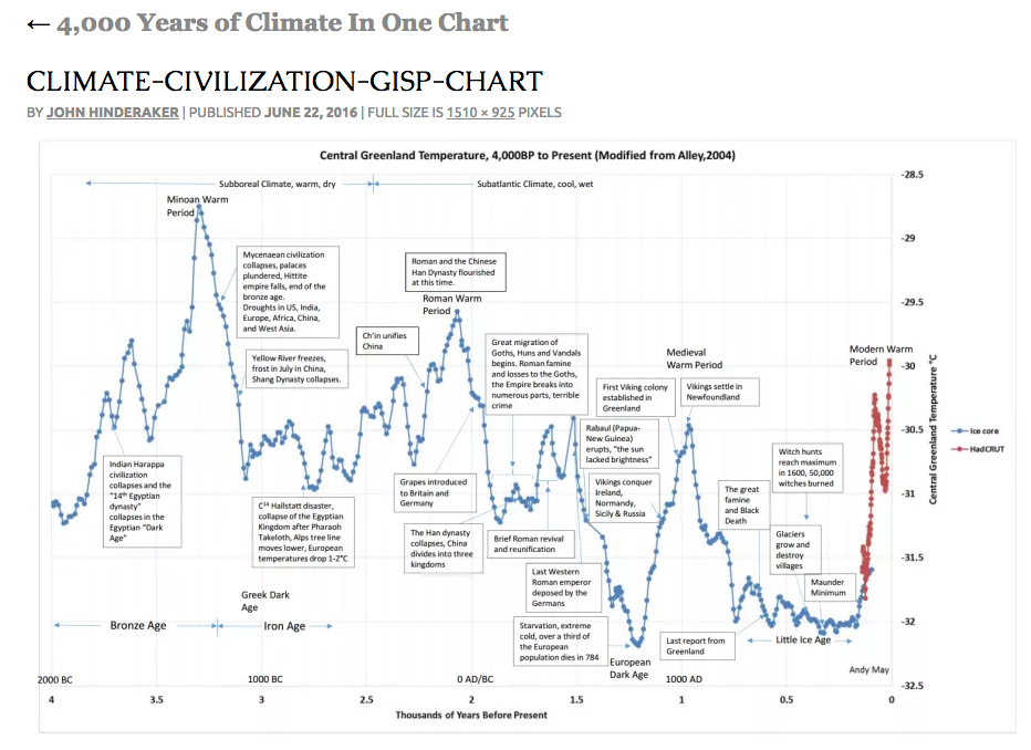
BTW, your last graph has someone else’s name on it, but I made that, see here: https://wattsupwiththat.com/2016/06/22/climate-and-human-civilization-for-the-past-4000-years/
Andy,
How dare that person?
I apologize. Thought it look familiar.
Yes. The Minoan is badly named, but that definitely warm interval shows up everywhere. As noted, the Egyptian at best only equaled the HCO, but probably didn’t globally. The Minoan however at least came close.
That’s why it’s possible to say that earth has been cooling for 3000 or 5000 years. The East Antarctic Ice Sheet quit retreating over 3000 years ago, during the Minoan, so-called. That’s based upon soil isotopes.
I would advice against concluding too much from Greenland or Antarctic ice cores. Greenland ice cores represent Greenland climate, and Greenland climate is known to differ from Northern Hemisphere climate quite a lot on a decadal to centennial scale. This is probably due to the polar vortex. When masses of very cold polar air invade Europe, Greenland warms due to the polar air being substituted by warmer air from mid-latitudes. Getting dates for historical Mediterranean climate periods from Greenland ice cores is risky business.
Javier,
I agree, but Greenland ice cores are still important.
The Minoan, Roman and Medieval WPs and intervening CPs show up everywhere, as do the counter-cyclic trends within the secular trends, such as the Sui-Tang warming during the Dark Ages CP.
Forrest: These are proxies and not measurements of temperature so computing error is difficult. I could do it with standard deviation or some variant of it, but that would just show the spread of the data and not real uncertainty. I’m open to ideas.
Temperatures were most likely not that stable in the past. In the alps melting glaciers release old trees every now and then. Typically these would be pine trees, which do well in high altitudes and low temperatures. However they will not grow beyond 2000m today, even though the treeline has gone up in the last century.
http://oekastatic.orf.at/static/images/site/oeka/20150626/pasterze_baum_katharina_aichhorn.5374067.jpg
So the 10 mio Dollar question is this: why are these old trees (3.500 – 7.000 years old) get released by a glacier at an altudite of about 2.250m? I mean these were large, solid trees, not like those small and crippled versions today would grow close to the treeline at 2.000. And glaciers do not move up hill, So unless some stone age folks played a trick on us, the treeline was like 400 – 500m higher then than it is today, which means accordingly higher temperatures of 4-5K.
Oops, I wanted to post this pic..
http://oekastatic.orf.at/static/images/site/oeka/20150626/pasterze_baum_michael_avian.5374068.jpg
This one is from Paul Homewood’s website
Physical evidence like wood remnants that can be radiocarbon-dated is much more convincing evidence than dodgy proxies or tree rings IM(non-scientist’s)O.
Columbia glacier Alaska as well… ?w=300&q=55&auto=format&usm=12&fit=max&s=081c44b31d98c54bea5e3c8d7deebf77
Erich @ June 6, 2017 at 11:56 am
Great photo, thanks. Do you have the glacier name or location and was any age dating done on the wood? Is the photo at 11:55 a distant view of the site?
@Alastair
“Do you have the glacier name or location and was any age dating done on the wood? Is the photo at 11:55 a distant view of the site?”
Well yes. The name of the glacier is “Pasterze”, located at the tallest mountain of Austria (Großglockner). Ironically the name means pasture, which may indicate what it was in medevial times. And yes, the first pic indicates the place the tree was found. I took it from this news report..
http://kaernten.orf.at/news/stories/2718069/
You may a lot more articles if you google “Zirbe” (german for pine tree) and “Pasterze”. You will need to handle the translation however.
Erich and Vukcevic, Great pictures! Thanks.
https://youtu.be/glplSyZM7uE
It’s admirable that some proxy records were prudently EXCLUDED from the determination of hemispheric anomalies, instead of being tendentiously ADJUSTED. Now if only manufacturers of land-station indices would learn to be as wise.
I remember from about the year 2004 that there was an Australian scientist boating around small lakes in SA and western Victoria getting mud cores for the last 20000 years.He said that once they had the pollen counts done we would have good proxies for the weather .I never heard any more,Has any one seen the results?
Patrick that was prof Patrick De Deckker who studied OZ paleo climate . Here is his video and transcript from the ABC show Catalyst in 2007.
http://www.abc.net.au/catalyst/stories/s1848641.htm
Since that time the Calvo et al study has used his data to show that southern OZ sst has been falling for the past 6,500 years. And they state that other OZ paleo studies show the same fall in temp over that period. And these studies agree with NZ and Antarctic temp record as well. Here’s the link and abstract to Calvo et al.
http://onlinelibrary.wiley.com/doi/10.1029/2007GL029937/full
Abstract
[1] Comparison of ice cores from Greenland and Antarctica shows an asynchronous two-step warming at these high latitudes during the Last Termination. However, the question whether this asynchrony extends to lower latitudes is unclear mainly due to the scarcity of paleorecords from the Southern Hemisphere. New data from a marine core collected off South Australia (∼36°S) allows a detailed reconstruction of sea-surface temperatures over the Last Termination. This confirms the existence of an Antarctic-type deglacial pattern and shows no indication of cooling associated with the Northern Hemisphere YD event. The SST record also provides a new comparison with the more extensive paleoclimatic data available from continental Australia. This shows a strong climatic link between onshore and offshore records for Australia and to Southern Hemisphere paleorecords. We also show a progressive SST drop over the last ∼6.5 kyr not seen before for the Australian region.
I am sure there is more than one group of Australian scientists investigating climate using lake bottom sediment cores. See for example this one:
Kemp, J., Radke, L. C., Olley, J., Juggins, S., & De Deckker, P. (2012). Holocene lake salinity changes in the Wimmera, southeastern Australia, provide evidence for millennial-scale climate variability. Quaternary Research, 77(1), 65-76.
http://www.academia.edu/download/44253021/Holocene_lake_salinity_changes_in_the_Wi20160331-25224-ajqsm7.pdf
Is any of these scientists the one you refer?
https://youtu.be/SbUsGnMUH2Y
“In 1990 I first traveled to Egypt, with the sole purpose of examining the Great Sphinx from a geological perspective. I assumed that the Egyptologists were correct in their dating, but soon I discovered that the geological evidence was not compatible with what the Egyptologists were saying. On the body of the Sphinx, and on the walls of the Sphinx Enclosure (the pit or hollow remaining after the Sphinx’s body was carved from the bedrock), I found heavy erosional features (seen in the accompanying photographs) that I concluded could only have been caused by rainfall and water runoff. The thing is, the Sphinx sits on the edge of the Sahara Desert and the region has been quite arid for the last 5000 years. Furthermore, various structures securely dated to the Old Kingdom show only erosion that was caused by wind and sand (very distinct from the water erosion). To make a long story short, I came to the conclusion that the oldest portions of the Great Sphinx, what I refer to as the core-body, must date back to an earlier period (at least 5000 B.C., and my latest research now points to the end of the last ice age), a time when the climate was very different and included more rain.”
http://www.robertschoch.com/sphinxcontent.html
With the recent additions of Gobekli tepe the perhaps Gulf of Cambay one never knows.
…..the great question is: How accurate are all sugested proxies?
One easy way to verify: Consult the Holocene series in
http://www.knowledgeminer.eu/climate-papers.html The Holocene is
covered in 8 parts. All parts show that every sizable cosmic impact
anywhere on the globe produces a sharp spiky temperature drop for
decades or centuries (depending on impact sze), followed by a sharp
temperature rebounce hot spike – the double spike impact pattern.
This is proven using the GISP2 Greenland series…..Now, since a cosmic
impact is a global event, this double spike MUST appear in all other
time series in the NH as well as in the SH.
By use of this double spike check, the accuracy of any time series
will show, JS.
“I would advice against concluding too much from Greenland or Antarctic ice cores. Greenland ice cores represent Greenland climate, and Greenland climate is known to differ from Northern Hemisphere climate quite a lot on a decadal to centennial scale. This is probably due to the polar vortex. When masses of very cold polar air invade Europe, Greenland warms due to the polar air being substituted by warmer air from mid-latitudes. Getting dates for historical Mediterranean climate periods from Greenland ice cores is risky business.” (Javier)
This statement is incorrect–Greenland climate does NOT “differ from Northern Hemisphere climate quite a lot.” There is excellent correlation between GISP2 ice core data, global glacier fluctuations, CET historic temp records, and various other proxy temp data. You can check these correlations yourself in the new Elsevier volume “Evidence-based Climate Science.”
Don Easterbrook has it correct: The GISP2 – Alley – series is the GOLD STANDARD,
because it
1.) reveals all double spike cold-warm temp oscillations after EACH cosmic
meteor impact (decadal to centennial, depending on crater size) +
2.) reveals temperature warm minispikes along the Holocene in the exact distance
of 62 years (the SIM-PDO-AMO cycle).
Other time series, which fulfill 1) and 2) are high quality, This Impact spike cycle and the 62 yr peak cycle check can easily be performed to endorse other time series.
Andy,
Could you please reduce the number of significant digits on your y-axes? Four decimal places suggests a level of precision that is unrealistic.
Jeff
ODP Hole 108-658C
Abstract:
“A detailed (ca. 100 yr resolution) and well dated (18 AMS 14C dates to 23 cal. ka BP) record of latest Pleistocene-Holocene variations in terrigenous (eolian) sediment deposition at ODP Site 658C off Cap Blanc, Mauritania documents very abrupt, large-scale changes in subtropical North African climate. ”
WR: this borehole is about eolian sediment. It reflects the abrupt change in landscape at the end of the African Humid Period. This change turned the Sahara into a desert after being covered by vegetation. Of course this resulted in a big transport of eolian material (= by wind transported) = fine sand and dust.
It is not clear to me how they can connect this sediment of land dust (but found on the sea bottom) with temperatures (fig. 11) of which it is not clear to me whether the temperatures are sea temperatures or land temperatures.
The article http://www.sciencedirect.com/science/article/pii/S0277379199000815 is paywalled.