Guest essay by Rud Istvan

Dr. Murry Salby has been getting substantial attention in the climate blogosphere, for two reasons. First is his theory that at least 2/3 of the observed increase in atmospheric CO2 is natural and temperature induced. Second are the circumstances surrounding his departure from U. Colorado and later termination from Macquarie University. This post covers the first and not the second, and is motivated by a very recent WUWT post on the mysteries of OCO-2, where the Salby theory was raised yet again in comments.
Background
Dr. Salby developed a substantial scientific reputation for work on upper atmosphere wave propagation and stratospheric ozone. He has published two textbooks, Atmospheric Physics (1996) and Physics of the Atmosphere and Climate (2012). His new theory that most of the increase in atmospheric CO2 is naturally temperature induced (NOT anthropogenic) is not published. He explicated it in a Hamburg lecture 18 April 2013, and a London lecture 17 March 2015. Both are available on YouTube. (Search his name to find, view, and critique them before reading on if you want to deep dive.) This post does not reproduce or critique his arguments in detail. (There are fundamental definitional, mathematical, and factual observation errors. Perhaps a more detailed companion post will follow detailing them with footnotes if this does not suffice.) This post only addresses whether his conclusions are supported by observations; it is a macro Feynman test rather than a Salby details deep dive.
Controversial CO2 Atmospheric Concentration Theory
The core of Salby’s theory is derived using CO2 data from MLO’s Keeling Curve since 1958, and satellite temperature data since 1979. (His few charts reaching back to 1880 contain acknowledged large uncertainties.) His theory builds off a simple observation, that in ‘official’ estimates of Earth’s carbon cycle budget, anthropogenic CO2 is only a small source compared to large natural sources and sinks. This is illustrated by IPCC AR4 WG1 figure 7.3.

He then deduces there must be rapidly responding temperature dependent natural CO2 net sources much greater than anthropogenic sources. This is a very questionable argument on short decadal time frames. Gore got it wrong, and Salby got it wrong. The ice core based CO2 lagged change to temperature is about 800 years, common sensically corresponding to the thermohaline circulation period. (For rigorous calculations on Salby’s decadal time scales using residency half-lives and efold times, see Eschenbach’s post at http://wattsupwiththat.com/2015/04/19/the-secret-life-of-half-life/

He observationally bolsters his conclusion by ‘showing’ that highest CO2 concentrations are over relatively uninhabited/unindustrialized regions like the Amazon basin, so must have natural origins. The following ‘observational’ figure is from his Hamburg lecture. Except it is completely disproved by OCO-2.

Critique
As Feynman said, observation trumps theory.
First, if Salby is right, the rise in atmospheric CO2 concentrations should have slowed or stopped because of the ‘pause’. They haven’t. They bear no short or long term relationship to one another. Since 2000, CO2 has increased about 35% on the 1958 Keeling curve base; temperatures haven’t (the pause). The seasonality of the northern hemisphere terrestrial photosynthetic sink is apparent in the Keeling curve, as is the temperature/CO2 discrepancy disproving Salby.

Second, satellites have NOT generally observed higher CO2 concentrations over uninhabited/ unindustrialized regions in past two decades. (The following NASA charts use AIRS IR sensors on various satellites to estimate gridded CO2 concentrations from peak CO2 OLR absorption wavelengths. The new OCO-2 data is even more stark.)

Third, Salby’s theory requires that land and/or sea serve as the temperature dependent CO2 net sources that ‘overwhelm’ anthropogenic CO2 emissions from fossil fuels and cement production. That is NOT true either; both land and sea have been serving as net sinks.
Terrestrial biomass (net primary productivity, NPP) is an increasing sink. This has been observed in multiple ways, including NASA AVHRR (1982-2009) and MODIS (2000-2009) ‘normalized difference vegetative index’ (NDVI). NDVI has been ground truthed by sampling NPP including both ‘roots and shoots’ by ecosystem. The terrestrial net biological sink has increased since 1980. It is not a source. The most recent paper is NASA’s 14% greening in 30 years, published 4/16/2016 and previously remarked at WUWT.

That leaves oceans. Biologically, oceans are a net carbon sink through photosynthesis and calcification. Satellites detect this through planktonic chlorophyll concentrations.

But there are certainly large ocean zones that are relatively barren (mainly from lack of iron fertilization in the form of dust). Those large blue barren swaths are where ocean water pCO2 and pH are monitored, precisely to minimize confounding biological sink influences recently explained on WUWT by Dr. Jim Steele. Could those also be a net source?
Barren ocean regions are mainly influenced Henry’s Law and Le Chatellier’s Principle. The first says partial pressures of ocean dissolved CO2 and atmospheric CO2 will equilibrate. The second partly says colder water stores more dissolved CO2. ARGO suggests the oceans are warming. Could Le Chatellier be stronger than Henry, in which case oceans could provide Salby’s requisite rapidly temperature dependent net natural source? There are two stations, Aloha 100 km north of Oahu (maintained by University of Hawaii and WHOI) and BATS off Bermuda (maintained by WHOI) where the hypothesis can be tested by observations. Both show even barren oceans are a net carbon sink since 1980. Barren ocean pH declines as pCO2 increases.

If there are no observational temperature dependent natural CO2 sources, and temperature dependent sinks (NH temperate terrestrial vegetation) increase with temperature, then Salby’s natural carbon dioxide theory cannot be true. It is falsified. Even before detailing his definitional, mathematical, and factual errors.
I love the circular logic of global warmists….not Dr. Murry Salby, it just reminded me of it
The recent warming can’t be explained by anything we know…..
…so we’re going to accredit it to something we know even less about….
…might as well blame it on the tooth fairy
The most recent paper is NASA’s 14% greening….
This will throw that off a tad….
“the world’s drylands host 40% more forests than thought, the team writes today in Science. That’s more than a 9% bump in total global forest coverage, or two-thirds the size of the Amazon.”
Earth’s forests grew 9% in a new satellite survey
http://www.sciencemag.org/news/2017/05/earths-forests-grew-9-new-satellite-survey
The two are not inconsistent. 14% is all earth. The new ‘forest’ is just drylands like the Sahel.
“It will also help scientists make more accurate estimates of how much carbon dioxide Earth’s trees are sucking out of the atmosphere—and how much of our fossil fuel emissions they’ll be able to handle in the future.”
ristvan
May 13, 2017 at 10:53 am
Ristvan……no matter what,,, the CO2 concentration trend is at the point that you should consider it as being unprecedented, aka no natural…..you will not have a standing hypothesis or theory to explain it, no body will have as the very ACC people will tell and acept .
As the ACC cabal will clearly say and prove to you when time be ripe for it…..you do not need a theory or hypothesis when the observation and the data show you clearly that the concentration CO2 trend is nearly at 420 ppm and showing that it will keep going up…
Remember, the scientific method,,,,, and the guy you called it a troll the other day when he point it out to you that you have not a hypothesis or theory……..and the ACCer will not need one either when at 420 ppm and especially in a cooling trend…..to claim that the anthropogenic CO2 is forcing the increase of the ppms……
and you and any one else at that point trying to complain and fight against the precautionary principle, aka something like a Paris treaty,,, will be just like peasants with pitchforks. trying to fight a very heavy armored and compact samurai force ….
The guy the other day was not a troll, even when it looked very much like one….already knew exactly what “he” was doing……
I am not sure but the last representation of Dr. Salby, did not look much like a theory or hypotheses to me, was more like a detailed analyses of the data and the observations, with a conclusive outcome……was more like a test crash or a attempt to falsify the AGW. How successful or good that was or is, is an entirely different matter but to me it did not seem like much of a hypothesis or a theory….wondering if that so, why would you try to paint it differently than it was or is…….!?
cheers
Whiten, am having a hard time comprehending your comment in order to respond. So lets take your comments in bites. CO2 concentration unprecedented depends on your time frame. C4 plants evolved because CO2 had got too low for dry place C3 plants to thrive. 85% of plant species are C3; evolutionary evidence that we are low rather than unprecidented high.
As to AGW, CO2 is a ghg. But, it could not have caused the temp rise from ~1920-1945 that is indistinguishable from ~1975-2000 (IPCC AR4 WG1 SPM fig. 8.2). So there is a very large attribution problem to AGW in the later period, upon which all CAGW rests.
As to precautionary principle, two observations. 1. The warmunist use is a 180 degree inversion of its original meaning, 2. The warmunist version is economic suicide.
As to Salby, yes he tried to refute AGW. And he failed miserably, as shown by my post– nevermind the details of how and why that two below demand (but if were fully as opposed to only partly in the post and comments), would still either not comprehend or object to). That way does not lie skeptical political success.
whiten
forgive me if I misinterpreted your post, but I read it as a stab at ristvan for his illustration of the, now, two studies that demonstrate the planet is greening.
First, I would suggest the green community ought to be cock a hoop over these studies and broadcasting them. Strangely, the very objective they have pursued for many years is now abandoned for political reasons.
Second, the precautionary principle is a scientific straight jacket. Whilst we are all desperate to avoid another Thalidomide event, how many more beneficial scientific programs were successful in pushing the boundaries of science without it. We would probably never have had penicillin if the precautionary principle were in operation at the time.
ristvan
May 13, 2017 at 1:50 pm
ristvan I can not blame it on you, the lack of understanding and getting my point……….especially when you keep listing the “pitchfork” arsenal you own……
At 420 ppm as the data and the observatiions stand, regardless of what temp trend or theories or whatever….the ppm trend stands as unprecedented in nature, according to the data and the observations…..
And if no one can reasonably quantify the outcome of such anthropogenic impact, either as good bad or nothing, then the precautionary principle applies on the point of considering the human CO2 emission reductions……and the only thing that matters then is the amount of the possible reduction, regardless of temps theories or what ever, CS, ECS, warming or any thing like that will not matter ristvan, only the “obvious” “truth” that ppms are very much forced by the anthropogenic CO2 emissions…end of the story at that point….as it clearly will be shown by the data and the observations…..
cheers
HotScot
May 13, 2017 at 2:04 pm
how many more beneficial scientific programs were successful in pushing the boundaries of science without it. We would probably never have had penicillin if the precautionary principle were in operation at the time.
—————————
Very good, in deed, I think any ACCer will applaud and accept it,,,,, having the anthropogenic CO2 emissions turned in to a scientific program, with a very much handling and controlling of it, as the program will require it, as a basic requirement.
Actual means and methods to reduced and manage it as required…..and as it being at this kind of point an international program it will require an international involvement with treaties like that of Paris……and a lot of “juice” and gravy to keep it running………….:) Virtually basically the same gravy train……
cheers
“His theory builds off a simple observation”
I know a theory can be built on an observation. How can one be built off an observation? Does it mean ignoring the observation?
RoHa
English is a wonderfully versatile language, to me in my version, they mean the same thing. To others and their variant of English they won’t.
We know since before the USA was founded that plants don´t grow without CO2. (Van Helmont, 1580-1644)
We know how plants capture CO2. (RuBisCo)
We know the RuBisCo capturing mechanism at atomic level.
We can reasonably quantify the increase of activity of RuBisCo as CO2 concentrations increase in vitro (Michaelis-Menten kinetics)
We have thousands of in vivo experiments proving that the in vitro ones are correct (www.co2science.org)
Those in vivo experiments are backed up in real life. (increase of world grain, vegetables, fruits productions per acre in the 20th century)
We have satellite confirmation that the planet is greening.
Yes, we can prove that increasing CO2 levels is good for plants.
BTW, In order to post your comments you had to click on the reply button, Just above said reply button there is a link that says: Earths-forests-grew-9-new-satellite-survey. (earth´s forests grew 9% in a new satellite survey). Are you ignoring the data you don´t like?
What does the ACC acronym mean?
Bob
My guess is that ACC means Anthropogenic Climate Change. YMMV.
RoHa
“Build on” means on top of something – The house is built on the foundations.
“Build off” means adjacent to something – The pier is built off the beach, often into deep water, which is where we seem to be with ACC.
The pause is meaningless in this context. As warming is driving CO2 out of the oceans, the atmospheric CO2 rises. It is ingenuous to assume that the outgassing goes to equilibrium as so much of the ocean is not in equilibrium with the surface temperature. Even if the pause lasted 40 years, outgassing would progress. No one knows how long it would take for the oceans to go to equilibrium as the climate never stays put in one place that long.
The lack of an equilibrium here is evidenced by the observation of lags in which CO2 always follows the temperature. For large CO2 swings, the lag is 600-800 years. In shorter time frames, it’s five to ten years.
Just as occurs with glaciers, as long as the temperature is above a certain temperature, melting occurs, it matters not whether, the warming goes up and down, melting will progress until temperatures drop low enough to favor glacier growth.
Higley7, your comment is an inverse variation on my first critique example, especially since Salby’s London talk guestimated a source response time on the order of 10 months to 1 year. So actually, the pause is highly relevant in the specific context of Salby’s two video claims.
higley7,
You are confusing the equilibrium of the atmosphere with the deep oceans with the equilibrium of the ocean surface.
The CO2 dynamic equilibrium (“steady state”) has an e-fold exchange rate of less than a year and any CO2 change in the atmosphere is followed by a change of CO2 and derivatives in the ocean surface within a few years.
Quantities in the atmosphere: ~800 GtC
Quantities in the ocean surface: ~1000 GtC
Temperature and CO2 exchanges between ocean surface and atmosphere are rapid and a matter of months to a few years for full equilibrium.
Temperature and CO2 exchanges with the deep oceans are of a different order and thanks to the sun, deep ocean cold upwelling is rapidly warmed up, releasing ~40 GtC/year as CO2. About the same quantity does sink into the deep oceans near the poles, the balance being slightly more sink than source, based on over 3 million seawater pCO2 measurements all over the oceans. See Feely e.a.:
https://www.pmel.noaa.gov/pubs/outstand/feel2331/exchange.shtml
and following sections.
For temperature, I don’t think you should wish any equilibration with the deep ocean waters at 3-5°C, as that effectively would reduce CO2 levels to where no C3 plants can survive. Neither is there any sign that returning waters of ~800 years ago contain more CO2 than in previous or later time periods.
“As warming is driving CO2 out of the oceans, the atmospheric CO2 rises”
Now we have to worry about run away CO2….another tipping point </snark
I would be more comfortable with any of these assertions if they included “When CO2 was measured as x, the rippling boundary heights for atmospheric layers in location specified surface conditions were y.”
Right you are, Latitude, …… not Dr. Murry Salby,
Excerpted text from above essay by Rud Istvan
Well “DUH”, then Salby’s theory is based in/on factual science, logical reasoning and intelligent deductions.
Of course it’s a “highly questionable argument”, but only for all those persons who do not understand (miseducated) and/or are incapable of recalling and associating the physical changes that occur in/with the earth’s surface ….. with the changing of the equinoxes (seasons).
The literal scientific fact is ……. that there is a “rapidly responding temperature dependent natural CO2 net source much greater than anthropogenic sources”.
And the aforesaid “natural CO2 net source” is the Southern Hemisphere’s ocean surface waters …. which the temperature there of, per se, “rapidly responds” on a 6-month seasonal cycle (bi-yearly).
Well “DUH”, there is NOT an electronic satellite in any part of earth’s atmosphere that is capable of actually seeing or detecting physical CO2 molecules floating freely in the atmosphere. The only thing those satellites can, per se, “see” (detect), is the IR radiation of a pre-defined frequency, ……. which NASA personnel then “assumes” said IR radiation frequency was emitted by CO2 molecules in a specific locale of the atmosphere.
But the problem is, as I see it, is the fact that the earth’s surface and/or atmospheric water molecules could be radiating that “pre-defined frequency” …… and/or …. the airborne CO2 molecule could be radiating IR in a non-defined frequency and thus the satellite would be, per se, “blind” to said CO2 IR emissions.
“DUH”, the “pause” was determined by the mathematically calculated “near-surface air temperature averages” ….. and those “near-surface air temperature” don’t have one iota of effect on atmospheric CO2 ppm quantities, ……. so don’t be wasting time and energy “looking for” a magical relationship to one another. And here is the graph with plotted data that proves, without any doubt, what I stated above, to wit:
http://i1019.photobucket.com/albums/af315/SamC_40/1979-2013UAHsatelliteglobalaveragetemperatures.png
But iffen you want to “see” the relationship between the bi-yearly (seasonal) cycling of atmospheric CO2 ppm as per the Keeling Curve graph and temperature …… then ya gotta be looking at the temperature of the ocean waters in the Southern Hemisphere.
The only thing that “is apparent” is the fact that you were mimicking a biological impossibility via you above statement.
Well, SURPRISE, SURPRISE, …….. given the fact said satellites are incapable of “observing” much of anything of a low-density gaseous nature that is residing in the atmosphere.
We know there’s no such thing as run away global warming…
..so, oddly enough, we also know there’s no such thing as run away global CO2
Very good, Latitude, …… I liked that.
Me thinks I’ll save it in one of my MS Word files as a “good quote” for repeating.
Samuel C Cogar May 13, 2017 at 4:09 pm
Well “DUH”, there is NOT an electronic satellite in any part of earth’s atmosphere that is capable of actually seeing or detecting physical CO2 molecules floating freely in the atmosphere. The only thing those satellites can, per se, “see” (detect), is the IR radiation of a pre-defined frequency, ……. which NASA personnel then “assumes” said IR radiation frequency was emitted by CO2 molecules in a specific locale of the atmosphere.
Except of course that’s not how the OCO-2 satellite measures the CO2 concentration in the atmosphere.
First, if Salby is right, the rise in atmospheric CO2 concentrations should have slowed or stopped because of the ‘pause’. They haven’t. They bear no short or long term relationship to one another
This is pretty much a falsification of Salby’s theory, although, of course, true believers will find excuses for this [and any other problem].
and some true believers claim the sun has no effect on the temperature.
Not relevant for this topic, so hold the snotty comments.
…LOL…Speaking of “snotty”, look in the mirror….
You do that !
Maybe Lief, you should put some effort into looking up the definition of “Snotty” !
you should look up the spelling of Leif.
Sorry. “Leif” is not found in any dictionary, no matter how much you value your own opinion…..
Try harder. “Put more effort into…”
http://www.dictionary.com/browse/leif
As for ‘snotty’: “having or showing a superior or conceited attitude”
The one making the comment [denoted as snotty] is the one to which the definition applies.
I apologize Dr.S….Auto correct error..…..I stand corrected !
lief in English means happily, gladly.
Source: https://en.wikipedia.org/wiki/I_before_E_except_after_C
[…But you forgot to add “… or when sounded like “A” as in neighbor and weigh.” .mod]
“A” as in neighbor and weigh
============
so Leif is pronounced layf not leaf
That is how my mother pronounced it. When I worked in Japan they insisted in calling me Raifu which is the closest they can come to the correct pronunciation. They tell me they can’t hear the difference.
I don’t know from Danish or any other Nordic language, but it’s dead simple in German. “Ei” sounds like short the pronoun “I” in English, while “ie” sounds like long “e”.
Since Leif Erikson was of Norwegian ancestry, though probably born in Iceland, but a speaker of Old Norse, I have no clue how to pronounce his name. When studying New World history, US kids hear both “Layf” and “Leaf”, usually the latter because at least it’s a word in English.
If only Tolkein were here to set us straight.
Did anyone stop to think that “Leif” is not an English word, and that English spelling and pronunciation rules would not apply?
IMO the faith-based pews are filled with CACA advocates, who can’t find a human fingerprint in climate, yet believe on blind faith alone that the culprit has to be those evil sinners against Nature, people.
who can’t find a human fingerprint in climate…
First they are made to believe that 400ppm is not some minuscule trace…then when it acts exactly like it should at that concentration…..they are bumfuzzled
It’s funny how innumerate Green activists wail about CO2 at over 400 ppm. Sounds so much scarier than 0.04%.
400,000 ppb is even more dangerous
Well, it was fun while it lasted. Now it’s over and something new must be hypothesized. Let’s see what reveals itself.
I query the phrase “long term”.
Meaning we haven’t been making detailed measurements for 1000 years. Let’s wait before we start talking about climate change, wait for 1000 years at least. After all, there’s nothing we can do about it, despite all the Cnuts and Gores..
So stupid. The model is not that CO2 is proportional to temperature anomaly, but that it is proportional to the integral of temperate anomaly.
When the critics cannot even be bothered to try to understand the argument, there is hardly any basis for agreement.
Bartemis, please reread the last sentance of the Background section of the post. I understand Slaby’s logic in detail, and where and why it fails. Eschenbach got part there in 2015 in his linked post. This essay is only about whether Salby’s conclusion might be observationally supported, not why and how Salby went logically wrong.
No, you are not even close. You are not even in the correct domain.
See longer critique of your article coming up soon from moderation.
1st thanks for Rud for writing on this topic. Could you publish your book as paperback?! I want a carbon sink in my library.
Bartemis,
In plain language you say: once seas get hot, they start leaking CO2 and the speed of the leak is dependent on the temperature anomaly?
Except not, because the partial pressure of CO2 has risen 30% (well, more, from 280 to 410 ppm), so of course the oceans have become a big net sink. At the same time, ocean temperature has barely nudged up.
Vegetation is also a net sink, so what is not? Coal (and oil, gas). If you go Salby, then you are basically forced to think vegetation is loosing mass and seas ‘boil’.
“In plain language you say: once seas get hot, they start leaking CO2 and the speed of the leak is dependent on the temperature anomaly?”
No, that is not the mechanism. That is a mechanism, but it does not amount to a whole lot.
It has more to do with the fact that, when the seas heat up, they stop carrying CO2 down.
There is a constant flow of CO2 laden waters upwelling in the tropics, and downwelling near the poles. Any imbalance between those flows must accumulate within the surface oceans. Rising temperature at the poles produces such an imbalance.
Hugs…a 30% increase in CO2 is not equal to a 30% increase in the atmospheric pressure…( CO2 is about 400 PPM. up by 30% since 1880)…not even a .004 increase in pressure..
Do you need me to calculate the partial pressure of CO2 in 1880 and 2017? Why?
Don’t say you mix % and unit-%. From 300 to 400 ppm is 100 ppm-units and 30%.
ristvan, where’s your point with Salby.
meanwhile –
https://www.google.at/search?q=sentance&oq=sentance&aqs=chrome.
Bartemis, sorry about misunderstanding. So you suggest there was an ocean sink in progress before, and it is now getting smaller because water warms up?
And human emissions simply don’t affect the balance and they roughly match the scale of atmospheric CO2 increase only by accident?
Well, that’s a hypothesis.
Hugs, wish that paperback carbon sink were possible. But even with print on demand to lower publisher risk, the Amazon price would have been $70-80 per copy because of all the color illustrations. So a cheap ebook it is, albeit in all ebook formats thanks to the publisher (iNook, Kindle, Nook, Kobo). Got that for his 40% cut. Good ebook news is, lots of footnote hot links, and footnote to websource links, and digital annotation capability.
Hugs @ May 13, 2017 at 12:55 pm
“And human emissions … roughly match the scale of atmospheric CO2 increase only by accident?”
What is we are talking about here? It very roughly matches 1/2 of the sum total of emissions over a century. Coincidence? You bet!
What continuing natural process do you know of where the outcome is in any way dependent on the sum total of inputs? Is the lake nearest you dependent on the sum total of rainfall since 1900? Is your bank balance anywhere close to your sum total of inputs over the years since you first opened it? Is the pavement outside your house as hot as the sum total of heat that went into it over the past several decades would make it? If you turn on the water at the faucet in your kitchen sink and leave it on for a week, will your house flood?
Of course not. In continuing, dynamic processes, you aren’t just filling a sealed bucket. You are feeding a process that keeps a given reservoir at a given level. You cannot increase that level by any amount proportionally greater than the proportion of the input you are feeding it.
Bartemis. If we have a sink with 100 gallons in it, and 1 gallon an hour entering from a tap and 1 gallon an hour leaving from the drain, we have stability. If we now add 1oz an hour extra, we will raise the level in the sink.
Occam’s razor would suggest that the raised level was because of the extra water added. Of course, it might be that the 1 gallon an hour entering had increased, but that introduces an extra couple of terms that Occam’s razor rejects – unless we have evidence for them.
It is reasonable that the increased level is attributed to the extra added water. If this hypothesis is to be rejected we need additional evidence.
It is reasonable to attibute the increased CO2 in the atmosphere to the extrac CO2 added by burning fossil fuels. Additional evidence required for other attributons is lacking.
..or the drain is clogged
No one knows enough about “sinks”…….
Butch,
For ideal gases, relative volume = partial pressure, thus ppmv = μatm pressure. With a slight difference: ppmv is usually expressed in dry air, while μatm is the real pressure in wet air. That makes a difference of a few % mainly at the ocean surface…
Bart:
What continuing natural process do you know of where the outcome is in any way dependent on the sum total of inputs?
Is the CO2 level in the atmosphere dependent of the sum of temperatures above a baseline?
Of course not, as a fixed change in temperature gives a fixed change in CO2 level in the atmosphere per Henry’s law: ~16 ppmv/K.
Bart’s theory completely ignores the effect of the increased CO2 pressure in the atmosphere, which is already 110 μatm above steady state, thus the average CO2 flux is from atmosphere into the oceans, not reverse. Which is observed. Thus Bart’s theory fails the main observation.
BTW, that the increase in the atmosphere is about half human emissions is just coincidence as a result of the slightly increasing CO2 emissions over time (a fourfold since 1958). So did the net sinks as result of the increased CO2 pressure in the atmosphere and thus the increase in the atmosphere.
seaice1 @ May 13, 2017 at 5:21 pm
” If we have a sink with 100 gallons in it, and 1 gallon an hour entering from a tap and 1 gallon an hour leaving from the drain, we have stability. If we now add 1oz an hour extra, we will raise the level in the sink.”
Under these circumstances, you will raise it thusly:
Settled level before extra added: L1 = K*1 gallon/hr
Settled level after extra added: L2 = K*(1 gallon/hr + 1 oz/hr) = K*1.0078 gallon/hr
% change in level: 1.0078/1 – 1 = 0.78%
” If this hypothesis is to be rejected we need additional evidence.”
Here is your evidence: If the level rose more than 0.78%, then part of the rise came from somewhere else. If it rose, say, 50%, then (50-0.78)/50 = 98.5% of the rise came from somewhere else.
Ferdinand Engelbeen @ May 14, 2017 at 4:48 am
“Of course not, as a fixed change in temperature gives a fixed change in CO2 level in the atmosphere per Henry’s law: ~16 ppmv/K.”
Henry’s Law only determines the ratio between atmosphere and ocean. It does not determine the absolute level.
“BTW, that the increase in the atmosphere is about half human emissions is just coincidence as a result of the slightly increasing CO2 emissions over time (a fourfold since 1958).”
It is 100% likely that any observed rise will be proportional to some other random number. This is not an amazing coincidence. It is a commonplace.
“So did the net sinks as result of the increased CO2 pressure in the atmosphere and thus the increase in the atmosphere.”
Ferdinand’s insistence that splitting the flow between the oceans and the atmosphere produces work to push CO2 into the downwelling waters is a perpetual motion scheme.
Bartemis
So true:-
The bigger the area of shallow water tropical seas under the influence of the Hadley Cell, the greater the production of warm dense saline water at the surface, the lower the gas carrying capacity of this seawater, the more CO2 is expelled into the atmosphere and the greater the outflow to depth of warm dense saline water.
Bower, A.S., Hunt, H.D. and Price, J.F., 2000. Character and dynamics of the Red Sea and Persian Gulf outflows. Journal of Geophysical Research: Oceans, 105(C3), pp.6387-6414.
In the geological past the east-west orientated Tethys Ocean with its shallow carbonate sediment rich epeiric seas ruled the climate of the warm ocean, high CO2 atmosphere, Cretaceous world. Now the linked north-south Atlantic Ocean, with its open connection from the Arctic Ocean to the latent heat polynya in the Southern Ocean Weddell Sea, rules the climate in the modern cold ocean, low CO2 atmosphere of our Ceonozoic world.
Bart:
Henry’s Law only determines the ratio between atmosphere and ocean. It does not determine the absolute level.
If the CO2 level/pressure in the oceans is known (expressed as pCO2(aq)), the ratio per Henry’s law determines the setpoint for the absolute level in the atmosphere: if the CO2 level/pressure in the atmosphere (expressed as pCO2(atm)) is higher, then CO2 will move from the atmosphere into the oceans or reverse if the pressure is lower. The resulting flux is directly proportional to the CO2 pressure difference (pCO2(atm) – pCO2(aq)) between the atmosphere and ocean surface.
The pressure difference is highly negative from atmosphere to ocean surface at the upwelling zones and highly positive at the sink zones. Net result: ~40 GtC of CO2 emitted near the equator, transported by the atmosphere and absorbed near the poles. Slightly more sink than source.
At any point of the ocean surface, an increase of 1 K in temperature increases the pCO2(aq) with ~16 μatm. An increase of ~16 ppmv in the atmosphere fully compensates for the increase in pCO2(aq), no matter if that is for one spot in the oceans or the full dynamics of the whole ocean surface.
This is not an amazing coincidence. It is a commonplace.
Not if the sinks behave as a simple linear process: in ratio to the pressure increase in the atmosphere above steady state, which they do in the past near 60 years…
insistence that splitting the flow between the oceans and the atmosphere produces work to push CO2 into the downwelling waters is a perpetual motion scheme.
Except that all the work is done by the CO2 pressure differences: pCO2(atm) is currently at ~400 μatm.
At the upwelling zones, pCO2(aq) is about 750 μatm. The 350 μatm difference does all the work to push 40 GtC/year CO2 from the ocean surface into the atmosphere. Potential energy transformed into kinetic energy…
The same at the sink zones: from 400 μatm down to 250 μatm.
The cold waters which sink near the poles return to the surface near the equator and are warmed up by the sun, increasing the pCO2(aq) again to ~750 μatm: that is your (near) perpetual energy machine at work…
“Not if the sinks behave as a simple linear process: in ratio to the pressure increase in the atmosphere above steady state, which they do in the past near 60 years…”
This is the nub of your problem. They do not act in ratio to the pressure increase above steady state. They react to the pressure, period.
That means they react to the sum total of natural and anthropogenic input. Since the anthropogenic input is variously estimated at 3-5% of the natural input, the anthropogenic share of the rise can only be in the range of 3-5%.
You take the “steady state” as a given, and then illegitimately decouple the anthropogenic input from the natural input. That makes your conception nonphysical.
“Except that all the work is done by the CO2 pressure differences: pCO2(atm) is currently at ~400 μatm.”
There is no work done there. Splitting the flow between the atmosphere and the oceans only means that, what is taken up by the atmosphere is that much less that is transported by the ocean currents. So, the downwelling sites have the added pressure of the atmosphere, but a reduced pressure from the ocean flow. The net effect is zero.
Bart:
They do not act in ratio to the pressure increase above steady state. They react to the pressure, period.
Bart, that doesn’t make any sense: the sinks react to the CO2 pressure (pCO2) difference between the atmosphere and seawater. If these are equal, nothing happens. At the sinks the waters have a lot lower pCO2 than the atmosphere: CO2 is absorbed. At the sources the waters have a lot higher pCO2 than the atmosphere: CO2 is released. The balance between these two is what changes the CO2 level in the atmosphere or reverse.
For the current ocean temperature the steady state is at 290 ppmv in the atmosphere. Any extra CO2 above 290 ppmv will reduce the influx and enhance the outflux.
That means they react to the sum total of natural and anthropogenic input. Since the anthropogenic input is variously estimated at 3-5% of the natural input
Completely wrong: the sinks don’t react on the natural or human inputs of one year, they react on the pressure difference between atmosphere and oceans. At steady state it doesn’t make any difference if the natural cycle fluxes are 40 or 400 GtC/year. If you add 5 ppmv CO2 in a year, the same pressure increase in the atmosphere will occur and the same net amount of CO2 will be absorbed by the oceans (less release + more sink), no matter the influxes.
That is Le Chatelier’s principle at work.
There is no work done there.
Wow Bart, a new escape plan? First you accuse me of creating a perpetuum mobile, now you say that no work is done. Of course work is done as kinetic energy is needed to release and absorb CO2, but the necessary potential energy comes from the sun.
Anyway what you say further is more interesting: What is released from the waters gets in the atmosphere and the waters that reach the sinks are more depleted and thus have a lower pCO2 at the same temperature. Agreed this time.
The interesting point is that an increase in temperature at every point in the ocean surface gives more CO2 in the atmosphere and thus less in the oceans. Before a new steady state is reached, the warmer sinks also receive less CO2 from the atmosphere, thus overall less CO2 sinks in the deep oceans than was upwelling.
The net effect is an increase in the atmosphere, not a “throttling” of the ocean sinks. That is only a null-operation when a new steady state is reached at ~16 ppmv/K…
“Bart, that doesn’t make any sense: the sinks react to the CO2 pressure (pCO2) difference between the atmosphere and seawater. If these are equal, nothing happens.”
The sinks react to total inflow, such that the steady state is proportional to the inflow, both natural and anthropogenic:
steady_state_combined = K*(NaturalInflow + AnthroInflow)
for some K. Take the AnthroInflow out, and you get
steady_state_Nat = K*NaturalInflow
Ratio of the two
steady_state_combined /steady_state_Nat = 1 + AnthroInflow/NaturalInflow
AnthroInflow/NaturalInflow is on the order of at most a few percent. Negligible.
“First you accuse me of creating a perpetuum mobile, now you say that no work is done.”
A perpetual motion machine of the first kind in one that does work with no input of energy. Work is required to overcome the added impedance to downflow induced by a temperature rise.
Bart:
The sinks react to total inflow, such that the steady state is proportional to the inflow, both natural and anthropogenic: steady_state_combined = K*(NaturalInflow + AnthroInflow)
No, most (sources and) sinks react on temperature, largely independent of what is in the atmosphere whatever the inputs (or outputs) at that moment. That gives the bulk of the in/out fluxes and a natural steady state of ~290 ppmv where NaturalInputs = NaturalOutputs, for the current average ocean surface temperature. That gives the residence time of ~5 years.
When the CO2 pressure in the atmosphere gets above the steady state of 290 ppmv, the ocean inputs are suppressed and the ocean (plus vegetation) outputs are increased. Thus part of the increased pressure in the atmosphere is removed. That is a much slower process than the temperature induced natural in/out fluxes: ~51 years decay rate.
Temperature changes are the driver for most natural inputs and outputs and the “setpoint” of the steady state.
Pressure changes are the driver for changes in the balance between inputs and outputs.
Bart:
A perpetual motion machine of the first kind in one that does work with no input of energy. Work is required to overcome the added impedance to downflow induced by a temperature rise.
If you are talking about the CO2 flux that goes into the deep together with the sinking waters: there is zero extra work needed to sink the CO2, as that doesn’t change in the waterflow itself between parcels of water: what is upwelling is ultimately downwelling no matter the temperature of the water.
Any work done is via the atmosphere: the pCO2 (= solar energy at the upwelling) difference is what drives CO2 out of the waters at the upwelling an drives CO2 into the waters at the sinks…
Snotty comment: Almost all discussion of CO2’s effect on global temperatures are irrelevant, since we live in the coolest period of the past 10,000 years, and in a cooler interglacial than the Eemian 125,000 years ago. Is the history of natural climate change irrelevant when it doesn’t suit the current fashion of climate scientism?
…+ 1,000… gold stars..stupid argument…
Well the question of relevance is of course how long it takes before we break records of 10,000 yrs, 100,000 yrs, 1,000,000 yrs, 10,000,000 yrs. If we’d do the last one in less than 200 years, I’d be scared. But it appears this is not probable atm.
Good point, majormike1. Let’s step back and look at the bigger picture:
The present is the key to understanding the past. And understanding the past is the key to looking forward to our future. Natural variability and the vastness of geologic timescales overwhelm popular human conception.
Sorry, graph courtesy of oz4caster at wordpress.
Good chart. Will save.
Leif, the premise of the question you answered was wrong to begin with:
http://www.woodfortrees.org/plot/uah/scale:0.3/plot/esrl-co2/derivative:1/mean:12/from:1979
In 2010 from WUWT, A study- the temperature rise has caused the co2 increase not the other way around by Lon Hocker:
“Conclusion
Using two well accepted data sets, a simple model can be used to show that the rise in CO2 is a result of the temperature anomaly, not the other way around. This is the exact opposite of the IPCC model that claims that rising CO2 causes the temperature anomaly.
We offer no explanation for why global temperatures are changing now or have changed in the past, but it seems abundantly clear that the recent temperature rise is not caused by the rise in CO2 levels.”
In 2014, First and second derivative atmospheric CO2 global surface temperature and_ENSO
“Abstract
A significant gap now of some 16 years in length has been shown to exist between the observed global surface temperature trend and that expected from the majority of climate simulations, and this gap is presently continuing to increase. For its own sake, and to enable better climate prediction for policy use, the reasons behind this mismatch need to be better understood. While an increasing number of possible causes have been proposed, the candidate causes have not yet converged. The standard model which is now displaying the disparity has it that temperature will rise roughly linearly with atmospheric CO2. However research also exists showing correlation between the interannual variability in the growth rate of atmospheric CO2 and temperature. Rate of change of CO2 had not been a causative mechanism for temperature because it was concluded that causality ran from temperature to rate of change of CO2. However more recent studies have found little or no evidence for temperature leading rate of change of CO2 but instead evidence for simultaneity. With this background, this paper reinvestigated the relationship between rate of change of CO2 and two of the major climate variables, atmospheric temperature and the El Niño–Southern Oscillation (ENSO). Using time series analysis in the form of dynamic regression modelling with autocorrelation correction, it is demonstrated that first-derivative CO2 leads temperature and that there is a highly statistically significant correlation between first-derivative CO2 and temperature. Further, a correlation is found for second-derivative CO2, with the Southern Oscillation Index, the atmospheric-pressure component of ENSO. This paper also demonstrates that both these correlations display Granger causality. It is shown that the first-derivative CO2 and climate model shows no trend mismatch in recent years. These results may contribute to the prediction of future trends for global temperature and ENSO. Interannual variability in the growth rate of atmospheric CO2 is standardly attributed to variability in the carbon sink capacity of the terrestrial biosphere. The terrestrial biosphere carbon sink is created by photosynthesis: a major way of measuring global terrestrial photosynthesis is by means of satellite measurements of vegetation reflectance, such as the Normalized Difference Vegetation Index (NDVI). This study finds a~close correlation between an increasing NDVI and the increasing climate model/temperature mismatch (as quantified by the difference between the trend in the level of CO2 and the trend in temperature).”
The warming/cooling of the ocean and CO2 are definitely related.
Leif, the premise of the question you answered was wrong to begin with
I didn’t answer any question…
http://www.woodfortrees.org/graph/uah/scale:0.3/plot/esrl-co2/derivative:1/mean:12/from:1979
“However more recent studies have found little or no evidence for temperature leading rate of change of CO2 but instead evidence for simultaneity.” from the abstract above.
Simultaneity is the operative concept.
Simultaneous with sea level change too.
What variable power drives ocean temps, sea level, and CO2 outgassing & absorption?
I interpreted “if Salby is right” as a question of theirs.
No biggie
Bob,
All what you look at in the work of Lon Hocker and others have the same problem: if you look at the derivatives, you have largely detrended the cause of the increase and inflated the noise around the trend. In the real world that noise is not more than +/-1.5 ppmv aroiund a trend of +80 ppmv.
From there Lon concludes that the residual trend in the derivative is caused by the same process as what caused the noise.
The problem is that you can’t conclude anything about the trend by looking only at the variability.
1. The residual trend in CO2 derivative is caused by a slightly quadratic increase of CO2 in the atmosphere. That is caused by the slightly quadratic increase of human emissions at twice the amounts of the increase in the atmosphere.
2. The variability is mostly caused by the effect of (ocean) temperatures on (tropical) vegetation (El Niño, Pinatubo). But vegetation is a proven, increasing sink for CO2, thus not the cause of the trend.
but if the lag is 800 years, how can it be falsified in 20?
…Tax Dollars ?
It sure isn’t 800yrs when your coca cola goes flat in an hour or so when it sits in a warm room.
This doesn’t make sense to me. From my time making homemade hooch, we brought the temperature of a solution containing alcohol to about 77 – 80 C, and held the temperature there. The solution continued evaporating the alcohol without raising the temperature further. The alcohol did not just suddenly evaporate. It occurred over a period of many hours. It would have evaporated at a lower temperature, but would have taken much, much longer.
I would assume CO2 in such a huge volume of water would also take a long time. Where am I wrong?
Simple. You have not watched the Salby vidoe lectures (or studied them if you, like Janice, did). You just provided another physical reason he is wrong.
come on, ristvan- vid or it didn’t happen.
pulling a mosher may be highly amusing to you, but i find it petulant and boring.
be better, no?
“Because of the enormous ocean thermal capacity, a lot of ocean heat capacity increase results in very LITTLE delta T. ” as you say.
cuts both ways
why would one expect a measurable change due to the pause?
KK,
Yes, what got left out of the presentation by Rud was the time to reach equilibration for a mass of upwelling water that is enriched in CO2, and constantly being replenished. It obviously doesn’t all flash off like popping open a warm soda drink. So, even if the global atmospheric temperature is constant for decades, it can be expected that outgassing will proceed at a faster rate than it did when the atmosphere was cooler.
KK,
The difference between the alcohol in your case and CO2 in the oceans is that there is practically no alcohol in the air above the liquid and thus the evaporation of alcohol is one-way. In the case of the (deep) oceans, there is a two-way exchange, as any release of CO2 from the oceans will increase the CO2 partial pressure in the atmosphere, thus pushing more CO2 back into the oceans. If nothing changes, that will lead to a dynamic equilibrium (“steady state”), where lots of CO2 do come in from upwelling deep ocean waters (~40 GtC/year) near the warm equator and lots of CO2 go out into the deep oceans (~40 GtC/year) near the poles.
For the current (weighted) average ocean surface temperature of ~15°C, the equilibrium is around 290 ppmv per Henry’s law. We are at 400 ppmv. That reduces the CO2 input at the equator somewhat and increases the output near the poles somewhat, thus slightly (~3 GtC/year) more CO2 sinks in the deep oceans than is released.
The reaction of the sinks to the increased CO2 pressure in the atmosphere is completely ignored by Salby, Bart and too many others…
“The reaction of the sinks to the increased CO2 pressure in the atmosphere is completely ignored by Salby, Bart and too many others…”
Because you cannot do work by mere splitting of flows, and you are proposing perpetual motion.
Bart,
Because you cannot do work by mere splitting of flows, and you are proposing perpetual motion.
If that was true, there wouldn’t be water evaporation and rain… Lots of energy are transported from equator to poles via water evaporation and clouds/rain.
The energy to move CO2 out of the oceans at the upwelling places comes from the sun and that extra CO2 pressure (potential energy) in the atmosphere is suffficient to push back about the same amount of CO2 into the cold ocean waters near the poles.
“Lots of energy are transported from equator to poles via water evaporation and clouds/rain.”
“…that extra CO2 pressure (potential energy) in the atmosphere is suffficient to push back about the same amount of CO2 into the cold ocean waters near the poles.”
The former process has an energy source, the Sun, which evaporates the water. The latter has no energy source. The CO2 diffuses from the waters, goes to the poles, and there diffuses back into the waters. It is only a splitting of the flow, with no net energy gained. The CO2 that diffuses to the atmosphere is that much less that is carried to the poles via ocean currents.
I made a good analogy to you the last time we traded opinions. You have a kitchen sink with the faucet turned on, such that the level of water in the sink reaches a specific level. Now, you take a chopping block and put it under the faucet, diverting part of the flow so that it drops in closer to the drain, so that it gets there a little faster. There is some small transient response, as the water sloshes a bit. But, in the end, it does nothing to increase the level of water in the sink.
Bart:
The latter has no energy source. The CO2 diffuses from the waters, goes to the poles, and there diffuses back into the waters.
There is energy needed for CO2 to escape from a liquid and absorbed back by a liquid. But that is in fact not relevant in the discussion. What is relevant is that all important changes occur in the atmosphere and these are influenced both by (ocean) temperatures and axtra (human) emissions.
You have a kitchen sink with the faucet turned on, such that the level of water in the sink reaches a specific level.
To which I responded that the analogy doesn’t fit the CO2 exchanges: the main sink/source fluxes are the result of temperature changes (seasonal) or differences (equator-poles). The main reaction of the sinks to any extra CO2 in the atmosphere is on the pressure change: different effects, different response times (~factor 10).
“The main reaction of the sinks to any extra CO2 in the atmosphere is on the pressure change:”
There is no net pressure change. Every parcel taken up by the atmosphere is that much less transported by the ocean currents.
This is very simple, Ferdinand. Let’s say I have pressure going as
dp/dt = -p/tau + u
The input u tends to increase the pressure. It does not matter if I split p into two components or not, the pressure is rising. That will increase the term p/tau, with will tend to relieve the pressure buildup.
If u is constant, p will eventually settle out to p = tau*u. But, if tau is very long, then it will take a long time to settle out, and in the intervening time, we will have
p := u
and, the pressure will continue building.
So, the diversion into the atmosphere is… a diversion. It has no impact on the question at hand. It is just a splitting of the flow.
I think you have made the mistake of thinking my model shows no buildup due to anthropogenic sources. That is not the case. It does. It is just that the impact is small relative to the impact from natural flows.
Because the time needed for deep ocean equilibration is long, both inputs accumulate in the surface system over a long time period. But, if anthropogenic inputs are 4% of the natural inputs, they are only responsible for about 4% of the observed rise. That is negligible, and can be ignored.
This is always the case then there is a dynamic balance – you cannot affect the outcome by a greater proportion than the proportion of your inputs.
Bart:
There is no net pressure change. Every parcel taken up by the atmosphere is that much less transported by the ocean currents.
There is no net pressure change from the natural inputs and outputs at steady state. That is the whole point.
In your formula:
dp/dt = -p/tau + u
dp/dt doesn’t depend of the natural inputs or outputs, as these are equal at steady state and natural u = zero. Thus u = human emissions and -p is the pressure difference between steady state (natural inputs = natural outputs) without human emissions. Tau is observed ~51 years
While only 4% of the inputs in mass (and 2% of the outputs in mass), human emissions make near all of the pressure change in the atmosphere…
What about endothermic mechanism of carbon dioxide dissolution and carbonic acid dissociation?
If the atmospheric temperature is flat and the heat is going into the ocean instead then CO2 outgassing would continue or have I missed something?
Yes, you missed something. Outgassing depends on delta T. True. Because of the enormous ocean thermal capacity, a lot of ocean heat capacity increase results in very LITTLE delta T. Look at measured ARGO delta T, not the computed delta quadrillion whatever heat therms to grasp this basic fact. It is another snooker play by warmunists.
ristvan
May 13, 2017 at 3:40 pm
Just for the sake of an exercise…would you think will be possible or reasonable to consider how long, years or millennia perhaps, will it take for the LITTLE delta T to increase and be “big” enough to count for the amount of outgassing required to fit the bill for the last century emissions of CO2, in regard to the CO2 concentration\s “observed” increase?!
Whiten,
With the current speed of increase, maybe 1 billion years, as the whole cold ocean interior need to reach over 22°C to give more CO2 in the atmosphere than 400 ppmv…
Ferdinand Engelbeen
May 14, 2017 at 5:27 am
Ferd, I really do envy your math….:)
cheers
Leif writes
I dont specifically know what Salby’s theorem is, but if you consider the greening of the planet as “drawing CO2 out of the oceans” by Henry’s law then as long as greening continues to lock CO2 into the vegetation even at the same temperature, the CO2 that is drawn out of the oceans will continue and ultimately the concentration in the atmosphere will increase, ratcheted up by the (primarily) NH seasons.
Clearly we’re putting more than enough CO2 out there ourselves to account for the increase so Salby does seem to have cause wrong if he’s considering today’s CO2 increases. Cause is something of a no brainer.
However the idea is an important one to take account of, I think.
lsvalgaard May 13, 2017 at 9:55 am
lsvalgaard, me thinks that one of the “other problems”, …… which I am not authorized to offer an excuse for, …….. is your above claim of “pretty much a falsification”, …… which I have to assume was a “self-admission” that you don’t have a clue about what you are criticizing ……. because iffen you were actually knowledgeable on the above subject matter in question, you would have explicitly stated your reason(s) for claiming said “falsification”.
And lsvalgaard, I address your above “pretty much a falsification” of the “pause” question that was first presented by Rud Istvan in my above posted response ‘here’ ….. and thus the reason I found your silly “pretty much” statement highly irritating.
Cheers, Sam C
which I have to assume was a “self-admission” that you don’t have a clue about what you are criticizing
Nonsense. Istcan notes that “First, if Salby is right, the rise in atmospheric CO2 concentrations should have slowed or stopped because of the ‘pause’. They haven’t”.
So Sakby is not right, unless he can explain why not. I see not such explanation. Do you?
lsvalgaard – May 13, 2017 at 6:51 pm
lsvalgaard, you are the one that was talking “nonsense” when you responded to Rud Istvan “nonsense”…. and you are still talking “nonsense”.
lsvalgaard, your 1st FUBAR mistake was when you assumed that Rud Istvan nonsensical comment that stipulated ….. “the rise in atmospheric CO2 concentrations should have slowed or stopped because of the ‘pause’” …. was a factually correct statement.
“WRONG”, ….. Istvan’s nonsensical claim about “rising” atmospheric CO2 not “pausing” in conjunction with the “pausing” of the rise in near-surface temperatures ….. was not based in/on actual, factual scientific evidence or observations, …… but was based in/on the CAGW “junk-science” claim that “increases in atmospheric CO2 directly cause increases in near-surface air temperatures”. And silly you, lsvalgaard, ….. agreed with Istvan.
And your 2nd FUBAR mistake, lsvalgaard, was your per se “demand” that Dr. Murry Salby was obligated to “explain why” Rud Istvan was wrong in claiming CO2 ppm rise should have “stalled” when the “pause” occurred.
And lsvalgaard, quit pretending “mental blindness”, it’s “a dog that won’t hunt”. To wit: “I see no such explanation. Do you?’
“YES”, lsvalgaard, …… I see/seen such an explanation, ….. because I posted said explanation, …. and I told you where you could see that explanation, …. but apparently your NIH attitude forced you to ignore said “explanation”.
Here, read it, to wit:
“DUH”, the “pause” was determined by the mathematically calculated “near-surface air temperature averages” ….. and those “near-surface air temperature” don’t have one iota of effect on atmospheric CO2 ppm quantities, ……. so don’t be wasting time and energy “looking for” a magical relationship to one another.
But iffen you want to “see” the relationship between the bi-yearly (seasonal) cycling of atmospheric CO2 ppm as per the Keeling Curve graph and temperature …… then ya gotta be looking at the temperature of the ocean waters in the Southern Hemisphere.
Too many assumptions…
My quote was
“First, if Salby is right, the rise in atmospheric CO2 concentrations should have slowed or stopped because of the ‘pause’. They haven’t”.”
If you have a problem with that go ask Istvan.
If Istvan and Salby are right my comment stands. If they are not, why even discuss the nonsense?
Everything is always qualified.
lsvalgaard – May 14, 2017 at 9:59 am
lsvalgaard, are you denying the fact that the following is a “copy” [w/included clarity punctuations] of your 1st posting to this thread in response to Istvan’s commentary wherein you specifically stated that Salby’s theory was falsified ….. via Istvan’s questioning “claim-of-factuality”, ….. to wit:
lsvalgaard – May 13, 2017 at 9:55 am
Did you note in your above that it was you who CLAIMED ….. falsification of Salby’s theory
lsvalgaard – May 14, 2017 at 9:59 am
If you have a problem with that go ask Istvan.”
I certainly did have a problem with that, as you damn well know I did …. and I addressed that problem to the “attention of Istvan” in my posting, ……. so why would someone who claims to be a Professional be asking such an ignorant question?
lsvalgaard – May 14, 2017 at 9:59 am
Now, again, just why would someone who claims to be a Professional be asking such an ignorant question ….. especially after that “someone” had already declared or adjudged Dr. Salby to be wrong?
Are your other Professional activities conducted similarly?
Scientists are allowed to [even encouraged to] disagree. Irritated activists like you have no influence on the road to wisdom.
For me, Salby is falsified. You may not think so. That is your problem, not mine.
And so bemoans: lsvalgaard – May 15, 2017 at 7:02 am
You should know, lsvalgaard, because you are a “prime example” and one (1) of a few posters hereon WUWT that my actual, factual, evidence based, science related commentary ….. has had no effect whatsoever on improving your science knowledge (wisdom) of earth’s natural world that you reside in/on.
“Whatever turns your crank”, …… lsvalgaard, …… and likewise “falsified” for several million other inhabitants who are utterly ignorant of the “specifics” of the biology of the natural world around them.
If you “think” Salby is falsified, …… then you should state science-based reason(s) for your thinking.
I figure Ferdinand E. will be supportive of your “thinking”.
Nuff for me ……. when the “horse refuses to drink the water” that they are led to.
There are comments that are worthy of a reasoned response, yours are, sadly, not.
That is not a falsification of the theory, since in chemistry there is a time lag in temperature-dependent solubility, often contingent on surface area.
Succinctly, once the temperature is set to a new level, CO2 will continue to off-gas until it is in equilibrium.
Salby does not take that into account, so why should we?
Frankly, I do not see how he could not take that into account. I only see that yours is a factually incorrect statement regarding the falsification of a temperature-dependent CO2 solubility theorem.
The hysteresis of CO2 equilibrium should only support an off-gassing theorem, as the temperature has not in fact gotten colder.
Where does Salby say that he carefully took that into account? He didn’t for the simple reason that it is not clear how to do this. How would you do it? My comment is not about what actually happens, but about what Salby says about it. So demonstrate that he took it into account. I would like to know.
Lira,
The CO2 exchanges between ocean surface and atmosphere are extremely fast, in the order of less than a year. Thus that equilibrium is settled within a few years, as can be seen in the increase of DIC (total inorganic carbon) in the ocean surface vs. CO2 in the atmosphere.
To reply to both of you, relative to the vast quantity of subsurface solvent (ocean water), there is a limited amount of interface surface area through which CO2 might off-gas. There then are ocean currents, layers, and temperature gradients beneath which may sequester and transport the solute.
Much of this can be demonstrated on a laboratory scale (or at home) with carbonated water of different temperatures relative to exposed surface areas. At basic value, you can even see where visible bubbles might become trapped.
Surface gas exchange, to an arbitrarily small layer, is not much relevant to the total oceanic presence, which will be brought in contact with the surface relative to time and agitation. If you wanted to model this, Reynolds number is often used. It’s somewhat analogous to gas mixing in the lungs being fast, but relatively slower is the total system of blood-gas turnover.
As for why Dr. Salby might not have explicitly stated this? (I’ve not read over his work in excruciating detail.) I would guess a similar reason to why I myself would not explicitly state it: It is extremely basic chemistry, and my research paper is not a student lecture on the topic. It would be sufficient to show the principle for the CO2 increase without having an exactitude on reservoir size. (Which would likely take running solubility and fluid dynamics work on every layer of the entire ocean.)
Lira,
In this case, you can simply ignore CO2 and temperature of the deep oceans, as one cycle between deep oceans and atmosphere needs about 800 years. One needs extreme changes in temperature and/or CO2 (+ derivatives) concentration in the deep oceans via the upwelling to have a discernable influence on short term (up to decades) CO2 or temperature of the ocean surface. For which is zero evidence.
All the variability where Salby’s theory is based on is on the short term: 1-3 years, the reaction of the CO2 rate of change on fast temperature changes (Pinatubo, El Niño). That is only at the ocean surface and in land vegetation.
Further, it doesn’t make a difference if you shake a 0.5, 1.0 or 1.5 liter bottle of Coke from the same batch: the pressure under the screw cap will be (near) the same for the same temperature. Thus lucky for us, only the temperature and CO2 concentration of the ocean surface is important. Equilibrium with the deep ocean temperatures (3-5°C) wouldn’t be so nice…
The equilibrium between ocean surface and atmosphere is very fast and per Henry’s law, the CO2 levels in the atmosphere should be ~290 ppmv for the current (area weighted) average ocean surface temperature. We are at 400 ppmv, thus the CO2 flux is from atmosphere into the oceans, not reverse, as is observed:
https://www.pmel.noaa.gov/pubs/outstand/feel2331/exchange.shtml
“One needs extreme changes in temperature and/or CO2 (+ derivatives) concentration in the deep oceans via the upwelling to have a discernable influence on short term (up to decades) CO2 or temperature of the ocean surface.”
Lira – get used to this. Ferdinand is very long on assertion, but short on actual foundation.
“The equilibrium between ocean surface and atmosphere is very fast and per Henry’s law, the CO2 levels in the atmosphere should be ~290 ppmv for the current (area weighted) average ocean surface temperature.”
What can I tell you? Ferdinand thinks the ocean is a bottle of Coke. No need to consider deep ocean currents. All the action happens at the top. By ignoring long term dynamics, he can come up any narrative he wants, and he thinks you should accept it because he says so.
Leif is a broken record. He cannot be reasoned with. No point in trying.
You don’t ‘reason’ with people. You present your scientific arguments without judging other people. Judge their arguments instead.
Mr. Englebeen, the ocean is not quantized into hard-limit layers, nor into absolute 800 year cycles, nor is the ‘pressure’ of a shaken bottle significantly relevant to the science of diffusion.
As I have explained to Dr. Svalgaard, it is simply a factually incorrect statement in chemical terms to state a ‘pause’ of temperature increase should result in a pause of off-gassing. There are non-temperature variables in the off-gas rate. It would only be a more relevant comment if the temperature of solvent had DECREASED.
Consequently, what Dr. Salby has or has not done is largely irrelevant: You cannot falsify his theory with first-order factual incorrectness.
That said, the ocean is a complex biosphere, and thus for a naturalistic explanation, I would expect a role for the microorganism constituent of it. Small temperature increases can yield larger scale metabolic responses, as anyone running a compost pile may be able to tell you. And of course, carbonates are a very large component in organism local pH management. Whether Dr. Salby discusses this possibility in detail, I’m not sure. But from what I’ve seen a naturalistic explanation is not so easily dismissed as attempted in this article.
Lira,
It is simply a factually incorrect statement in chemical terms to state a ‘pause’ of temperature increase should result in a pause of off-gassing. There are non-temperature variables in the off-gas rate.
The variability of temperature (or more accurate, the dT/dt variability) explains over 60% of the dCO2/dt variability, thus one can expect that the pause has some effect on the rate of change. But nevertheless not that important as that is a discussion over the noise around the trend, not the cause of the trend itself…
Further, most of the exchanges between atmosphere and oceans (CO2, O2, temperature) are fast with the “mixed layer”, the upper 100-200 meters of the oceans where most of biolife is. Deeper parts hardly play a role, except for the biological pump and the deep ocean exchanges at a restricted number of places…
Re: “First, if Salby is right, the rise in atmospheric CO2 concentrations should have slowed or stopped because of the ‘pause’.”
I cannot reconcile this statement in the original post with the earlier “The ice core based CO2 lagged change to temperature is about 800 years, common sensically corresponding to the thermohaline circulation period.”
If the latter is well established, and I think it is, then the former must be wrong. No? Given the slow rate of conductance into the deep oceans, an 800 year lag seems easy to explain but surely the process would be progressive. Degassing would start rising within decades and keep increasing until the ocean temperature had stabilized. In view of this we might expect to see measurable degassing after 250 years. (i.e. since about 1750A.D.)
Steve,
If we may assume that ice cores give a reasonable impression of historical CO2 levels, these were ~290 ppmv about 800 years ago. Seems quite difficult to push that to 400 ppmv now with upwelling waters of that period…
And don’t wish for any temperature equilibrium with the deep ocean waters: at 3-5°C, CO2 levels would drop so much that most C3 plants (all trees, a lot of crops), would die off…
However, if the lag be 800 years, as seems reasonable, then the rise in CO2 since c. AD 1850 could be reflecting the Medieval Warm Period. Before Mann tried to get rid of it, that interval was dated from c. AD 900 to 1400, with a central peak of around 150 years.
IMO most of the recent increase in CO2 is however from human sources. My guess is about 70 ppm of the alleged 120 ppm gain in beneficial plant food since 1850, but possibly a larger share.
The lag, if any, is very poorly defined in any case.
Essay Cause and Effect in ebook Blowing Smoke discusses the lag in some depth, along with several laughable attempts to disappear it for warmunist purposes. Shakun 2012 was the most serious (his PhD and Nature paper) and in several ways the most fundamentally flawed. Amazing that it got through peer review.
On every post from WUWT lately, you find a way to promote your own Ebook….pathetic…
[well if he was was making a line to Amazon, you’d have a point, but he isn’t, so you don’t – Anthony]
…Very good point, but it just seems repetitive…(maybe my point of view is bias because I already went there and read it..) ?
Nope. You make the false assumption that CO2 has a major effect upon temperature. It doesn’t. It’s an effect of temperature increase, not a cause.
I’d have thought that that was obvious.
After the first 100 or 200 ppm, I should have said.
Even if it is all due to humans, it is demonstrably a good thing. Of course, we need an accurate description (not model) of the “carbon cycle” which we don’t have.
..Robert of Ottawa, Canada….I simply cannot understand why ANY Canadian in the “Frozen North” would want it to be colder than it already is…I was raised in Blind River, Ontario as a child….During winter in the North. everything was simply shut down !
Well done Robert, only a couple more stages to go.
Yes, the order-1000 year lag time between when water last sees the northern atmosphere and when it upwells and warms again at the equator is a deeply confounding factor. What were conditions of the atmosphere then? How did dust and biota falling through the water column in the interim affect dissolved carbon? All will have an effect, but it may take a long, long time.
pochas94,
CO2 levels in the atmosphere 800 years ago were around 280 ppmv. I don’t see any reason that these CO2 levels of 800 years ago would increase the current CO2 levels to over 400 ppmv…
CO2 levels over the past 800,000 years follow temperature with a surprising linear ratio of about 16 ppmv/K, as per Henry’s law for CO2 in seawater. Only since 1bout 1850 CO2 levels start in lockstep with human emissions. Pure coincidence?
Chimp May 13, 2017 at 9:57 am
Chimp, according to the following, …. human sources for “recent increase in atmospheric CO2” ….. don’t have leg to stand on, ….. wooden or otherwise, to wit:
Samuel,
But the termites, like the poor, we have had with us alway.
@Chimp
And what do you think a warmer climate does to termites?
Maybe they like it and grow more colonies? Therefore produding more CO2? There is never a ‘ceterus paribus’ situation in nature. Everything changes and everything is interdependent.
Samuel,
Termites use wood that incorporated its CO2 from the same atmosphere where it is released again, only a few years to a few decades before.
The current biosphere, including termites, is a net sink for CO2, the earth is greening, despite the number of termites, animals, humans and other (indirect) veggies…
There, Ferdinand, ……. I fixed it for you.
Do you have references for this? It seems like the world could use a few less termites, or perhaps we could harness their production.
Humans reading such things consume more aspirin, driving an increase in production, which consumes CO2. Homeostasis in action.
R. Shearer – May 14, 2017 at 12:53 pm
R. Shearer, …. I guess iffen you don’t know how to use the Internet and the Google program for finding answers to simple little questions ……. then it’s probably OK iffen I do it for you …… so here is the reference you asked for, to wit:
http://www.nytimes.com/1982/10/31/us/termite-gas-exceeds-smokestack-pollution.html
“so here is the reference you asked for”
That NY Times article is about the Zimmerman paper that was probably overestimating termite emissions by at least a factor of 10.
And even then it doesn’t agree with your claim that termites produce 10 times as much CO2 as all fossil fuels. The article only says more than twice as much – and that’s compared emissions in the 80s.
Samuel,
Termites don’t increase the CO2 levels in the atmosphere today for the simple reason that vegetation absorbs more CO2 than all bacteria, fungi, insects and animals together release.
Humans do increase the CO2 levels in the atmosphere today for the simple reason that the production of new coal, oil and gas absorbs less CO2 than humans release from the ancient atmosphere.
Ferdinand, …… have you un-plugged your refrigerator/freezer?
If not, why not, …… you already told me that cool, …… cold ,,,,,,,, and freezing temperatures will not prevent the microbial decomposition of the dead biomass foods that you have placed in your refrigerator/freezer for “safe keeping”.
Or did I misunderstand you …… and that “safe keeping” thingy you claimed was to prevent your pack of pet pooches (dogs) from eating the food(s) you have saved for you, your wife and kids?
Chimp,
The fact that there has never been a runaway hothouse from which Earth did not recover (Tipping Point), suggests that, at the very least, the temperature sensitivity to CO2 is much less than generally claimed. Moreover, there appears to be some sort of negative feedback loop that corrects for temperature changes over the long term. One possible explanation is that CO2 isn’t even driving the temperature, but is a result of it. That is, it takes a millennium for temperature changes to work through the system, and once out of equilibrium, outgassing will continue for hundreds of years, as long as the Earth isn’t quickly plunged into another ice age by some exogenous forcing.
Consider the following: In the absence of anthropogenic CO2, the oceans might supply CO2 at a greater rate than what they currently do. That is, anthropogenic CO2 is moderating the rate at which CO2 outgases in a warming world. Therefore, the correlation with anthropogenic CO2 may be a spurious correlation.
Clyde,
I couldn’t agree more.
But that doesn’t mean that most of the apparent CO2 gain over the past 167 years isn’t from human activities.
Per IPCC AR5 Figure 6.1 prior to year 1750 CO2 represented about 1.26% of the total biospheric carbon balance (589/46,713). After mankind’s contributions, 67 % fossil fuel and cement – 33% land use changes, atmospheric CO2 increased to about 1.77% of the total biosphere carbon balance (829/46,713). This represents a shift of 0.51% from all the collected stores, ocean outgassing, carbonates, carbohydrates, etc. not just mankind, to the atmosphere. A 0.51% rearrangement of 46,713 Gt of stores and 100s of Gt annual fluxes doesn’t impress me as measurable let alone actionable, attributable, or significant.
And in some other words.
Earth’s carbon cycle contains 46,713 Gt (E15 gr) +/- 850 Gt (+/- 1.8%) of stores and reservoirs with a couple hundred fluxes Gt/y (+/- ??) flowing among those reservoirs. Mankind’s gross contribution over 260 years was 555 Gt or 1.2%. (IPCC AR5 Fig 6.1) Mankind’s net contribution, 240 Gt or 0.53%, (dry labbed by IPCC to make the numbers work) to this bubbling, churning caldron of carbon/carbon dioxide is 4 Gt/y +/- 96%. (IPCC AR5 Table 6.1) Seems relatively trivial to me. IPCC et. al. says natural variations can’t explain the increase in CO2. With these tiny percentages and high levels of uncertainty how would anybody even know? BTW fossil fuel between 1750 and 2011 represented 0.34% of the biospheric carbon cycle.
Nicholas,
How much carbon is in reservoirs is not of the slightest interest, as long as there is no exchange between the reservoirs.
How much carbon is exchanged between the reservoirs is not of the slightest interest, as long as the ins and outs are equal.
What is of interest is the balance: 9 GtC/year human emissions in, 4.5 GtC/year increase in the atmosphere, thus the natural unbalance is -4.5 +/- 3 GtC/year, including year by year natural variability. Nature is a net and increasing sink for CO2 already near 60 years of accurate measurements and thus not the cause of the increase, no matter how one tortures the data…
BTW, accuracy of human emissions: +/- 0.5 GtC (based on sales – taxes) and CO2 measurements: +/- 0.4 GtC. Accurate enough to show that nature is a net sink for near 60 years, no matter if the natural cycles were 10 GtC/year, 150 GtC/year ot 1000 GtC/year in and out…
Some questions which may cast doubt on the accuracy of some of the figures:
1. Do the figures for “human emissions” take account of CO2 from respiration particularly in view of world population growth ?
2. Do the figures for “human emissions” take account of fuel burnt that is not taxed and may not be fossil fuel anyway but still produces CO2 during combustion? For example where I live most households are burning 3 – 6 tonnes of wood per annum, usually from their own land = no records, no taxes.
3. Do the figures for “human emissions” take account of burning for reasons other than heating/cooking? For example burning of waste/rubbish which may range from personal garden refuse to larger scale burning of collected waste from many households. There is also burning as a recovery process for, e.g. copper from cable scrap.
4. Do the figures for “human emissions” take account of wind turbines catching fire? OK, maybe a little /s but have you seen how much smoke and flames you get from a “good ‘un”?
5. Do the figures for “human emissions” take account of the respiration of our dogs/cats in view of the increasing popularity of having a pet and therefore this is probably increasing at a greater rate than population in some countries?
I suspect that the crude calculation of fossil fuel related CO2 derived from records of oil/coal sales , etc is highly likely to be a significant under estimate of the actual amount of CO2 which is human produced. A significant percentage may be simply due to human population growth and associated growth in related activities which produce net CO2 entirely independent of the fossil fuel contribution. Has anyone ever seen a study of this point?
Reverend,
Your points 1), 2) and 5) are part of the biosphere, as what is emitted/exhaled as CO2 was taken out of the atmosphere some months to decades before. In average that gives a slight sink for CO2: about 1 GtC/year more CO2 removed by photosynthesis than is returned by burning wood or eating/digesting/exhaling…
For point 3) depends of what is used is recent organics or fossil organics. In the first case, it is part of the biocycle an in the second case, the average energy use to produce plastics, metals, paper,… is included in fossil fuel use, the energy recuperation from burning wastes, as far as I know, not.
About point 4), I only hope that much more of these bird and bat killers burn down…
So natural sources don’t explain the increasing CO2 and rising CO2 can’t explain the pause. Good thing the science is settled or there would be a lot of questions to be sorted out.
So, carbon dioxide and temperature are uncorrelated outside of laboratory conditions (and carbonated drinks), implying that there are other unidentified and uncharacterized sources and processes that regulate both.
Have no informed opinion about Salby’s theories, but do have graphical demonstration of global temperature – CO2 connection http://www.woodfortrees.org/plot/esrl-co2/mean:12/scale:0.2/isolate:60/plot/hadcrut4gl/isolate:60/mean:12/from:1961
Even more striking for the tropics http://www.woodfortrees.org/plot/esrl-co2/mean:12/scale:0.2/isolate:60/plot/hadcrut4tr/isolate:60/mean:12/from:1961
Oh stop it…..your graph clearly shows the CO2 follows temps very quickly…. 😉
…..tropics can’t find the hot spot either
“global temperature – CO2 connection”
What it does show is the scale factor – 0.2. That is, a 1°C rise in temp corresponds to a 5 ppmv increase. We’ve seen a 120 ppmv increase since pre-industrial – that would need a 24°C rise in temperature.
No, it wouldn’t. It is NOT A PROPORTIONAL RELATIONSHIP!
It was in the plot he showed.
Hi Nick; what does the 120 ppmv CO2 mean for temperature?
Bart,
Of course it is a proportional relationship or you are violating Henry’s law for the solubility of CO2 in seawater…
No, Ferdinand. Henry’s Law only determines the ratio of partition. It does not say anything about the absolute concentration which is rising as a result of the temperature change.
Bart:
Henry’s Law only determines the ratio of partition. It does not say anything about the absolute concentration which is rising as a result of the temperature change.
Of course it does. For a fixed temperature, the fixed ratio between CO2 in seawater and the atmosphere gives a fixed absolute concentration in the atmosphere. At 15°C ocean surface that is ~290 ppmv in the atmosphere.
If the temperature of a liquid increases the solubility of any gas is reduced, because the internal pressure to escape from the liquid increases. That is measurable and for CO2 in seawater, the internal pressure of CO2 (called fugacity) increases with about 16 μatm/K. With a fixed ratio, the increase in the atmosphere also would reach ~16 ppmv/K for a new equilibrium.
“With a fixed ratio, the increase in the atmosphere also would reach ~16 ppmv/K for a new equilibrium.”
That is only the short term equlibration. But, the overall level in the surface system, partitioned between surface oceans and atmosphere, is increased, because there is less transported out of the system via downwelling.
Henry’s Law has nothing to say about that long term buildup, except for how it will be partitioned.
Bart,
the overall level in the surface system, partitioned between surface oceans and atmosphere, is increased, because there is less transported out of the system via downwelling.
That is during the transition to a new steady state. When the increase in the atmosphere reaches ~16 ppmv more CO2 per K temperature change, the original CO2 downfluxes are reestablished and as much CO2 sinks in the deep as before (and as much is released at the sources as before), with the help of the higher CO2 level in the atmosphere.
“When the increase in the atmosphere reaches ~16 ppmv more CO2 per K temperature change, the original CO2 downfluxes are reestablished…”
Splitting the flow does not push more CO2 into the downwelling. This is a perpetual motion scheme.
Bart,
Splitting the flow does not push more CO2 into the downwelling. This is a perpetual motion scheme.
No, the increased pressure of CO2 in the atmosphere pushes more CO2 in the downwelling. That is the point. The energy needed is supplied by the increased pCO2 due to warmer ocean temperatures in the upwelling zones.
These plots are closely related to Humlum’s analsyis as seen at his website climate4you.com and his published paper from 2013. He concluded from these extensive data analyses that “(6) CO2 released from anthropogene sources apparently has little influence on the observed changes in atmospheric CO2, and changes in atmospheric CO2 are not tracking changes in human emissions.”
Harde 2017 consulted Salby and incorporated many of his thoughts and concludes “Our analysis of the carbon cycle, which exclusively uses data for the CO2 concentrations and fluxes as published in AR5, shows that also a completely different interpretation of these data is possible, this in
complete conformity with all observations and natural causalities.” The alternate conclusion they find
is the one described by Salby.
This alternate conclusion does not need to assume saturated sinks at the beginning of the industrial age or fractionated residence times that cannot be measured but are in conflict with 36 published estimates of CO2 residence time developed using 6 different methods between 1957 and 1992. The IPCC residence curve keeps 40% of fossil fuel CO2 in the atmosphere for over 100 years where these studies all cluster around 5 to10 years.
DMA,
Common error of too many skeptics to mix residence time with e-fold decay rate. The residence time has nothing to do with the decay rate of any extra CO2 injection in the atmosphere above dynamic equilibrium per Henry’s law. The residence time is mainly seasonal and temperature driven. The decay rate of any extra CO2 in the atmosphere is pressure driven. The residence time is ~5 years, the e-fold decay rate is ~51 years.
See Willis’excellent post:
http://www.wattsupwiththat.com/2015/04/19/the-secret-life-of-half-life/
It is the same difference as between the turnover of goods (and thus capital) in a factory and the gain (or loss) that the same factory makes. Somewhat related, but largely independent of each other.
Both Humlum and Harde made the same error of (indirectly) using the residence time, which is of no value in the calculation of how long it takes to remove some extra CO2 out of the atmosphere…
The IPCC makes use of the Bern model, which includes large residual amounts of CO2 in the atmosphere, due to saturation of the deep oceans and vegetation, for which is not the slightest indication…
Have no informed opinion about Salby’s theories, but do have graphical demonstration of global temperature – CO2 connection http://www.woodfortrees.org/plot/esrl-co2/mean:12/scale:0.2/isolate:60/plot/hadcrut4gl/isolate:60/mean:12/from:1961
Even more striking for the tropics http://www.woodfortrees.org/plot/esrl-co2/mean:12/scale:0.2/isolate:60/plot/hadcrut4tr/isolate:60/mean:12/from:1961
Mmm; 3 compared to 4:
http://www.woodfortrees.org/plot/esrl-co2/mean:12/scale:0.2/isolate:60/plot/hadcrut4gl/isolate:60/mean:12/from:1961
Nice write up Rudd.
And all this time I though PC02 was related to my computers anthropogenic footprint!
The CDIAC plot shows CO2 in ppmv vs the annual rate of emission. I think like should be compared with like – CO2 with cumulative emission, or annual rates of change. Here, from here, is the plot of CO2 in ppmv vs cumulative emissions. The mass balance can be compared, and there is a fairly constant airborne fraction (reasons here), so that only about half remains in the air. But it is very clear that, with all the natural annual cycling over the pre-industrial years, no nett change occurred. It was just the same carbon going through various phases, as it still does. The rise in CO2 in ppmv started with our emissions (initially land clearing), and tracked it throughout.
the plot of CO2 in ppmv
Sorry, it compares both atmospheric C and cumulative emissions in Gtons C.
no nett change occurred…so it was limiting
The temperature relationship shows a better match since reliable CO2 estimates became available.
http://i1136.photobucket.com/albums/n488/Bartemis/tempco2_zpsmgkycbdj.png
I must admit it looks neat. But. Correlation in not causation.
The unambiguous correlation is in the rate domain. Human emissions do not track with anything like this level of detail.
http://i1136.photobucket.com/albums/n488/Bartemis/scale022_zps2rnyhcl6.png
The problem is that HadCRU’s books have been cooked to show such a relationship.
The RSS correlation below however is more convincing, even though its series has now also joined the bogus, cooked book, climate consensus collective Borg.
Well, then, check out UAH:
http://woodfortrees.org/plot/esrl-co2/derivative/mean:12/from:1979/plot/uah6/offset:0.73/scale:0.2
HadCRU’s books have been slightly cooked, though they are far less well done than GISS. But, they have not been cooking them to show a relationship between temperature and the rate of change of CO2.
Bartemis,
It’s clear that the fluctuations in CO2 follow temperature, but that doesn’t mean that no accumulation from human sources has occurred. My own guess at the man-made portion is lower than, say, Ferdinand’s estimate.
“It’s clear that the fluctuations in CO2 follow temperature, but that doesn’t mean that no accumulation from human sources has occurred.”
Occam’s Razor. The temperature relationship fully accounts for the rise. Why assume something you do not need?
BTW, human inputs indubitably account for some of the rise. But, it is a negligible level, probably on the order of maybe 3-5%, if estimates of the relative size of anthropogenic inputs to natural inputs are accurate.
Bartemis,
IMO there is a need to explain what I consider to be higher than naturally occurring CO2. The temperature increase since 1850 has been minor compared to the CO2 gain, assuming that pre-1958 estimates are in the ballpark.
“…assuming that pre-1958 estimates are in the ballpark.”
Why would you assume that? I sure don’t.
It is a moot question. Since 1958, when the best, most accurate, direct measurements of CO2 became available, the rate of change of CO2 to temperature relationship has held with extraordinarily high fidelity. In that era, the concentration rose from about 315 ppmv to the current 400 or so ppmv. If it had stayed at 315 ppmv, we would hardly even care. IMO, we can safely discount the pre-MLO era has having little to no relevance.
Bartemis,
“The temperature relationship shows a better match”
Consider what is plotted. One is carbon added versus carbon measured, both jn Gtons. The other is carbon measured vs the integral of Southern Hemisphere temperature, with a specially chosen offset first, then a chosen matching factor, then another offset. All with no physical explanation, and restricted to just a 60-year period. There are enough degrees of freedom in that matching to turn the straight line y=x into any section of any parabola.
No, Nick, there are not. The quadratic component of the absolute CO2 level is directly related to the linear component of the rate of change. It comes from the trend in temperature, not from any arbitrary fitted parameter.
That is precisely the key element that establishes that the rise is overwhelmingly due to temperature. The trend in temperature fits the quadratic term in CO2, when it is scaled to match the variability. Emissions also have a linear growth that would accumulate into a quadratic term. But, since the quadratic component is already explained essentially in total by the temperature dependent term, there is little to no room for it. Ergo, human inputs cannot be contributing significantly to the outcome.
“It comes from the trend in temperature, not from any arbitrary fitted parameter.”
So what is the 0.22 multiplier on temperature?
Bartemis,
“The temperature relationship shows a better match since reliable CO2 estimates became available.”
Just to show how easily these nonsense correlations can be produced, I played around in WFT. I took Crutem4, but scaled it by zero and offset by 1. That seems to be the only way to produce a constant 1 – I tried random etc, but they only go to year 2000. Then I integrated, offset by 500 and integrated again, then scaled by 0.000146. The same number of fitted choice parameters as you have, and it is just a parabola. No climate information at all. The result plotted against ERSL Co2 is here:
http://www.woodfortrees.org/plot/crutem4vgl/from:1958/to:2016/scale/offset:1/integral/offset:500/integral/scale:0.000146/offset:314/plot/esrl-co2/mean:24
or pictured here:
What mechanisms justify the offsets?
“What mechanisms justify the offsets?”
Good question. In my case it was just fitting, as I believe it is in Bart’s.
Bartemis’ plot shows CO2 rising with the *Integral* of temperature, which implies that if temperatures stay constant from now on, CO2 will continue to rise indefinitely at the same rate. I think that is somewhat unlikely, to say the least.
It is also worth noting that Bartemis’ plot suggests CO2 levels would remain constant if temperatures were about that seen in the 1890s (determined by the scaling of 0.22 and the first offset of 0.1). This implies that during glacial periods, which were (IIRC) about 4 degrees cooler than that, CO2 levels would have rapidly plummeted below zero ppm, which is of course absurd. So this is at best only a local approximation, where one approximately exponential signal (integrated temperature) has been fitted to another approximately exponential signal (atmospheric CO2) using three free parameters. It is not surprise that this can be done, as Nick demonstrated.
Bart,
As usual…
The correlation is between the variabilities, as that is mainly the effect of temperature on (tropical) vegetation. The trend is NOT caused by vegetation, as that is a net sink for CO2. Thus while most variability is caused by temperature, that is just noise and the trend is caused by the twice as high human emissions.
The combination of emissions, increase in the atmosphere (and thus net sink rate) gives exactly the same plot as yours, where temperature is only a minor player for the trend:
http://www.ferdinand-engelbeen.be/klimaat/klim_img/had_co2_emiss_nat_deriv.jpg
Ferdinand, would you please further an explanation of the red line in your plot. (what exactly does it mean, how did you calculate it?) Thanx…
Nick Stokes @ May 13, 2017 at 7:42 pm
You integrated twice! Of course you can get a quadratic term if you integrate a constant twice.
Now, plot the derivative:
http://www.woodfortrees.org/plot/crutem4vgl/from:1958/to:2016/scale:0.000001/offset:1/integral/offset:500/integral/scale:0.000146/offset:314/derivative/plot/esrl-co2/mean:24/derivative
Oops! Doesn’t match the variations AT ALL!
This is p*** poor, Nick. Are you purposefully just trying to muddy the waters?
jorgekafkazar May 13, 2017 at 9:39 pm
“What mechanisms justify the offsets?”
1) offset for equilibrium temperature anomaly – temperature anomaly baseline is arbitrary, so there is no reason for it to have physical significance in the first place
2) offset for integration constant
dikranmarsupial @ May 14, 2017 at 2:19 am
“…which implies that if temperatures stay constant from now on, CO2 will continue to rise indefinitely at the same rate.”
For a time, until other dynamics assert themselves. This is a linearized model which is expected to hold locally in time, and holds very well for the period under observation. This is standard engineering practice. If we have a system
dx/dt = -x/tau + u
for some input u and time constant tau. If the period of observation is much less than tau, then the equation becomes approximately
dx/dt := u
and, we can use that as the model for near term analysis. But, the actual system is not ultimately unbounded for u of one sign, as this one would be.
Ferdinand Engelbeen @ May 14, 2017 at 6:20 am
Your model is nonphysical, as you are taking a natural equilibrium state as a given, and decoupling the equilibrium dynamics from the anthropogenic input.
“Offsets let us plot two data sets on the same chart. “
Your examples are of known, defined scale factors (eg 1.800000). These are fitted, and they do more than put the two graphs on the same page. They optimise the fit. And because the integration suppresses most of the variation detail, they basically just match up the low order moments. That was the point of my demo that just applying fitting multipliers and offsets could match a straight line of unit slope to the CO2 curve, just as well as doing the same with HADCRUT 4 SH. The scale matches the curvature (2nd moment), then the offset added before integration matches the slope, then the final offset matches the intercept. They are all the parameters you need to fit a quadratic.
Nick:
So what IS the scaling factor between ppmv and °C ?
Bartemis wrote “You [Nick] integrated twice! Of course you can get a quadratic term if you integrate a constant twice.”
Yes, of course he did. Nick multiplied temperature by 0 and added 1 to get a constant and then integrated it to get a linearly increasing signal. Nick’s point was that with three free parameters you can easily get a match to atmospheric CO2 by integrating any signal with an approximately linear increase. Perhaps you ought to try and understand the point being made before dismissing it. Of course it doesn’t explain the variations, but then again, as Nick’s example shows integrated temperature doesn’t necessarily explain the long term increase.
“This is a linearized model which is expected to hold locally in time, and holds very well for the period under observation. “
Yes, of course it does, with three free parameters you can get an equally good fit by integrating more or less any linearly increasing signal, as Nick demonstrated, so it means precisely nothing.
Nick Stokes @ May 14, 2017 at 5:41 pm
This is either dishonest or incompetent.
Fonzie,
It is getting problematic here to follow all the discussions…
As I remember well (it is already years ago…), it is the combination of the direct influence of temperature on the variability in CO2 rate of change (4-5 ppmv/K), to match the amplitudes at one side and human emissions minus the calculated sink rate on the other side.
The calculated sink rate is the result of the fixed ratio over the past near 60 years between observed sink rate and the CO2 levels in the atmosphere above the calculated equilibrium for the momentary temperature with base 290 in 1960 plus the temperature anomaly at 16 ppmv/K.
The fixed ratio is currently ~2.15 ppmv/year for 110 ppmv above equilibrium and was quite constant over the past near 60 years.
The result you see is that almost all the trend is from human emissions minus the net sink rate and that almost all variability is from the temperature impact on (tropical) vegetation plus in part ocean temperatures (but vegetation wins the contest)…
Bart:
Your model is nonphysical, as you are taking a natural equilibrium state as a given, and decoupling the equilibrium dynamics from the anthropogenic input.
Bart, the natural equilibrium state IS a given, as proven by 800,000 years of ice cores, showing a fixed ratio between temperature (proxy) and CO2 levels (measured). It IS a given per Henry’s law. confirmed by over three million seawater samples.
All what I have decoupled is that natural variability and trend have nothing to do with each other as is proven by the opposite CO2 and δ13C changes: changes in (tropical) vegetation are the main cause of the CO2 rate of change variability, induced by ocean temperature variability. But vegetation is a net, increasing sink for CO2 over periods longer than 1-3 years, thus NOT the cause of the increase in dCO2/dt or CO2 in the atmosphere… That are human emissions, not temperature.
http://www.ferdinand-engelbeen.be/klimaat/klim_img/temp_dco2_d13C_mlo.jpg
BTW, as you can see there is a lag between dCO2/dt and dT/dt, thus the integral relationship is between dT/dt and CO2, not between T and CO2. Unfortunately for you (and Salby’s) theory, dT/dt has no trend, only a small offset, good for a few ppmv CO2 after integration…
“…the natural equilibrium state IS a given…”
Sure, sure. It’s magic!
No, Ferdinand. A natural equilibrium does not just exist for no reason. There has to be a dynamical relationship that establishes it. And, that dynamical relationship is going to apply to any anthropogenic inputs as well.
Bart:
There has to be a dynamical relationship that establishes it. And, that dynamical relationship is going to apply to any anthropogenic inputs as well.
The dynamic relationship between ocean surface and atmosphere for the ocean temperature is 16 ppmv/K with a current steady state setpoint of ~290 ppmv.
The dynamic relationship for the removal of any excess CO2 in the atmosphere above that dynamic setpoint has a tau of ~51 years, No matter the origin of that excess.
Excess compared to what? How do you know there is an “excess”? How did the magical equilibrium level come about?
The answer: it is established by a balance between inflow and outflow. We cannot shift that balance by any greater proportion than our proportion of additional inflow. If we attempted to, we would be opposed by the very same forces that oppose the natural inflow.
That is what is missing from your model. That is what makes it nonphysical.
Bart:
Excess compared to what? How do you know there is an “excess”? How did the magical equilibrium level come about?
There is nothing “magical” about the steady state between the ocean surface and the atmosphere. For every temperature of the ocean surface, there is a fixed level in the atmosphere where ocean surface and atmosphere are in equilibrium per Henry’s law. It doesn’t matter if that is for a single sample in a lab or for the average temperature and the full dynamics of the total ocean, including sinks and sources.
The answer: it is established by a balance between inflow and outflow. We cannot shift that balance by any greater proportion than our proportion of additional inflow. If we attempted to, we would be opposed by the very same forces that oppose the natural inflow.
That is where you go wrong. The main in/out fluxes are directly cuase by temperature differences, while the removal of any injection of extra CO2 is only possible by pressure differences.
In the case of the oceans, the main influx is at the upwelling, where the warming up of the deep ocean waters gives a boost to CO2 to enter the atmosphere. The opposite happens at the sink side. The quantities involved are directly proportional to the pCO2 difference between atmosphere and ocean surface or reverse, thus mainly by local temperatures. Total flux between sinks and sources ~40 GtC/year via the atmosphere, in steady state at ~290 ppmv in the atmosphere for an average 15°C ocean surface temperature.
The outflux is not dependent of the influx of any particular year, but depends of the pCO2 difference between atmosphere and sinking waters, the former of course is influenced by the inputs.
Take an extra CO2 input of volcanoes or humans and the pCO2 in the atmosphere increases. That will influence both the incoming fluxes and the outgoing fluxes, proportional to the pressure increase in the atmosphere. Completely independent of the influx or outflux of that moment. The difference between the new influx and outflux is what net sinks into the deep oceans (and vegetation). That is measured at current ~2.15 ppmv/year.
Humans add ~4.5 ppmv/year, the difference remains in the atmosphere.
Atlantic Ocean CO2 uptake reduced by weakening of the meridional overturning circulation
http://www.nature.com/ngeo/journal/v6/n2/abs/ngeo1680.html
“…there is a fixed level in the atmosphere where ocean surface and atmosphere are in equilibrium per Henry’s law.”
That only tells us the ratio, not the absolute level. It does not say anything about the content or distribution within the oceans, or how it came to be.
“The main in/out fluxes are directly cuase by temperature differences, while the removal of any injection of extra CO2 is only possible by pressure differences.”
You are still only talking about the atmospheric/ocean interface. This is only a small part of the flow problem. Oceanic transport is not instantaneous, and it is not simple. It is very long term, and very complex. You are dismissing it as though it were of no consequence, treating the vastness of the oceans as though it were a shallow pond.
You are like the proverbial blind man, who feels the elephant’s trunk, and declares that an elephant is a long, sinuous animal, much like a snake. You have not even begun to explore the other parts of the elephant.
Nick,
Thanks for an informational comment. Mostly I agree, but will mention this:
“The rise in CO2 in ppmv started with our emissions (initially land clearing),…”
The chart indicates land clearing started about 1850. It is possible to argue that land clearing has been going on for much longer. So, two examples only:
Recent — Pennsylvania’s big cut
http://explorepahistory.com/story.php?storyId=1-9-E&chapter=1
Not so recent — forests of the Lebanon cedar
https://en.wikipedia.org/wiki/Cedars_of_God
Nick,
You surely are expert at producing nonsense correlations.
John,
” It is possible to argue that land clearing has been going on for much longer.”
Yes, I think so too. I plotted Houghton’s data, which started in 1850. There is some indication of an earlier small rise in atmospheric CO2.
Land effects conceivably go back at least 2000 years in the Amazon.
https://www.sciencedaily.com/releases/2017/02/170207092752.htm
Nick
These depictions of the ice core CO2 records were used to argue that the increase had to be human caused. There are multiple refutations of there accuracy for absolute CO2 content. They are good indicators of changes but because of the mechanics of the ice formations and diffusion in the ice layers and liquid water found in the ice layers down to -70C they will always show less than the maximum concentration for the period they represent. Stomata counts show over 360 PPM 10,000yrs ago. High quality chemical analysis show over 350 PPM during the 19ty and early 20th century.
DMA,
Please, don’t repeat what Jaworowski said in 1992, which was all refuted in 1996 by the work of Etheridge e.a. on three ice cores at Law Dome.
Ice cores are excellent indicators of ancient CO2 levels, the only drawback is that they are always a mix of several years, depending of the local snow accumulation rate. Between 10 years resolution over the past 150 years and 560 years resolution over the past 800,000 years. Repeatability +/- 1.2 ppmv (1 sigma) for Law Dome, maximum 5 ppmv difference for the same average gas age for ice cores with extreme differences in temperature and accumulation rate.
Including an overlap of ~20 years (1960-1980) between ice core data and direct measurements at the South Pole. See further:
http://www.ferdinand-engelbeen.be/klimaat/jaworowski.html
I had years of discussion with the late Ernst Beck about the historical data. While the accuracy was reasonable (+/- 10 ppmv), where was measured was problematic: midst of towns, under, inbetween and over growing plants, midst of forests… Completely unsuited for “background” CO2 levels of that period. See:
http://www.ferdinand-engelbeen.be/klimaat/beck_data.html
Ferdinand Engelbeen
May 14, 2017 at 6:34 am
Ice cores are excellent indicators of ancient CO2 levels, the only drawback is that they are always a mix of several years, depending of the local snow accumulation rate.
——————————
No, the ice core data in the way you address these data are far from excellent indicators, and the drawbacks far much more serious then you try to imply and make believe…
These data confuse and contradict each other very significantly over the CO2 concentration and the temperatures….
Sorry Engelbeen, if you use your basic math carefully you may just realize that for your self……
All data is subject to drawbacks due to pollution and contamination of the samples by other natural signals other than the ones that the data tries to represent, and also due to raw data processes that can not fully and accurately count for all needed adjustments and interpretation of such data…….some thing like in the case of the actual CO2 residence time in atmosphere.
Remember the ice core data is just that, it is in no way atmospheric data…
cheers
Whiten,
CO2 in ice core bubbles from Law Dome were measured with the same equipment as direct measurements in the atmosphere at the surface, in firn and show the same CO2 levels in the period 1960-1980 as direct measurements at the South Pole.
Thus if you have concrete findings why and when these data are so far contaminated that they can’t be reliably used, I am all ear.
There are more discussions about the proxies in the ice core used for temperature indication. Mostly δD and δ18O in the ice. The heavier isotopes show some increase with higher temperatures where water is evaporated and where the same water vapor directly freezes to snow and what of these is more important. And that ratio also may shift between glacial and interglacial periods.
That makes that the polar 8 ppmv/K CO2 change probably is 16 ppmv/K globally (another ongoing discussion…). Anyway, the CO2/T ratio between glacial and interglacial periods didn’t change over 8 interglacials, each some 100,000 years apart and 16 ppmv/K is in the ball park of Henry’s law for CO2 in seawater.
Ferdinand Engelbeen
May 15, 2017 at 12:51 pm
Do you realise how silly your argument is?
The bred and butter about icecore data is the long term paleo climate representation of climatic parameters.
Trying to validate the worthiness and accuracy of such data in long term by relying in a period of 20 years between 1960 to 1980, to me is beyond silly….
Still icecore data do confuse and contradict among…. and are highly polluted by other signals other than the ones that supposedly to be representing the temp and CO2 concentration variation….
There is Greenland icecore data that due to such discrepancy are considered and deemed arbitrary invalid because, because these data very clearly contradict other ice core data and other proxies..to a very high degree of violation……
Also very long term ice core data in general do contradict clearly shorter term icecore data to a point that the picture for the same event, like an interglacial, is completely in two different ranges that do not even slightly overlap…as at the very least expected , when it comes to climatic parameters that these icecore data suppose to reflect and mirror….A huge unacceptable error………
Considering your knowledge, I am surprised that you still do not get it, with all you math magic!
cheers
Whiten,
Greenland ice cores are far more contaminated by a combination of sea salts and frequent acidic dust from nearby Icelandic volcanoes. That gives in-situ formation of CO2. Therefore the CO2 results can’t be used as unreliable in many cases. The same bubbles contain CH4 and these match the Antarctic CH4 data.
As far as I know, ice cores show a trapped overlap with each other, each longer one “bootstrapped” with the next longer one with a longer resolution. The first two (Law Dome) show 150 years with a resolution of less than a decade and match 20 years with direct measurements at the South Pole. The next get ~1.000 years back in time and match the 150 years of the first, etc.
The main problem is in calculating the average age of the gas composition, mostly (verified) modelling (firn densification model), but the shapes of the CO2 changes in general are identical.
Land clearing has been occurring for millennia by axe and burning; it’s just another ad hoc hypothesis dreamed up by the alarmists to explain another of the anomalies (inconsistencies) in their neat settled science™.
The pre-1958 CO2 trend aside, if land clearing was responsible for the purported CO2-driven instrumental surface temperature trend prior to ~1945 (that can’t be explained by emissions), it could also explain the similar trend post-1945:
http://www.climate4you.com/images/HadCRUT3%20GlobalMonthlyTempSince1850%20WithSatellitePeriod.gif
You may NOT combine ice core proxies and MLO instrument data. That’s just flat FRAUD.
Nicholas,
You may combine ice core CO2 with instrument data, as ice core CO2 are direct measurements, not proxies. Even done with the same instrument by Etheridge for CO2 in ice, firn and atmosphere for the Law Dome data.
There is a 20-year overlap between Law Dome CO2 data and direct measurements at the South Pole:
http://www.ferdinand-engelbeen.be/klimaat/klim_img/law_dome_sp_co2.jpg
Ice core measurements are one or two steps removed from the original sample air, i.e., they are proxies.
R. Shearer,
Depends of the definition of “proxy”.
In general a “proxy” is some variable which is influenced by the variable of interest. Like three ring widths or density for temperature and stomata data for CO2 levels. These need calibration over some periods with the variable of interest.
In general the proxy variable is not only influenced by the variable of interest, but also by other variables like precipitation in the case of tree rings and local/regional CO2 sinks/sources in the case of stomata data. Or by non-linear responses, maximum responses,…
That is not the case for CO2 in ice core bubbles. While there are corrections needed, like a correction for the increase of the heavier isotopes and molecules at the bottom of stagnant air (based on the change in 15N/14N ratio), these corrections are not higher than 1% of the measured value, which is a direct measurement of the variable of interest.
Thus in my opinion ice core CO2 is not a “proxy” in the same sense as most proxies, but may be called a “proxy” because it doesn’t reflect the CO2 levels of a particular moment in time or even a particular year, but a skewed (to more recent years) average mix of several years of air.
Nice flatline; what was temp doing during this period?
How does one know for sure? in any case, he is of retirement age, and one should not hold that against him.
An employed person, usually, has many required distractions from a main interest. Once or twice we had to fill out forms detailing activities by each 15 minutes. Some useless meetings are required or expected.
Once retired a person can focus on that main interest, or other things one did not have time to do when a salary is being earned.
We recommend it.
Thank you, Rud Istvan.
You are welcome, fellow traveller, presumably from Europe. Auf Deutsch, Vielen Dank.
I am from the Netherlands and I try to teach the Dutch skeptics on carbon cycle basics.
Together with his Flemish fellow traveller (but have been working 34 years in The Netherlands in the chemical industry)…
Hi Ferdinand, you too thank you very much for your input here!
Thanks Rud
I believe skeptics have made several unforced errors by refusing to call out BS. This refusal has allowed other to easily and credibly tar you all with one big brush.
Rud avoids this simple mistake.
Many folks will pick up any skeptical argument as long as it is merely opposed to accepted science.
So lets start here. With The Core of climate science ( CAGW is another thing )
1. C02 is a GHG. Yes virginia, C02 like water vapor is a GHG. GHGs make the planet warmer than it would
be otherwise not cooler. YET skeptics continue to entertain and allow sky dragon types to spread their
nonsense. Do yourself a favor and distance yourself from these clowns. That means Pro actively countering their BS.
2. Humans are responsive for the rise in C02. Yes throw salby under the bus. You cannot on one hand demand
that folks follow the scientific method, publish their data and code, and then let SALBY lead your charge
since he refuses to actually do science or publish results. YouTube videos are not science.
3. The world is in fact warming. Yup. The temperature record is not a hoax. There was an LIA it was cooler in the past. It is warmer now. That sentence and the concept of a ‘global’ temperature has an operational meaning.
folks might reasonably disagree about a few tenths here and there, but the LIA was in fact real. It is in fact warmer.
4. Prior to the intrusion of politics into science, scientists did in fact ( 1896, 1938) Predict that adding C02 would warm the planet. They did not predict it would cool the planet. They did not predict it would warm everywhere or even warm monotonically year in and year out because the recognize that other factors can temporarily work against this warming trend. The increased warming we see is evidence FOR the theory it is not Evidence AGAINST the theory. but the pause!!! All other things being equal an increase in my salary causes my bank balance to go up. Last month it went down. Hospital bills. This “disconnect” between salary and balance doesnt mean that in general an increase in salary will NOT lead to an increase in balance.
What left? Whats left are the real questions, the open questions in the science. These are the questions where skeptics COULD IN FACT have an impact on the trajectory of the science and the conversation. If you stay mired down in arguing 1-4, at some point people will stop talking to you as your position is akin to flat earthers.
What are the real questions left.
1. How much will we emit in the future
2. How much will we warm
3. Should we and can we do anything.
The temperature record is not a hoax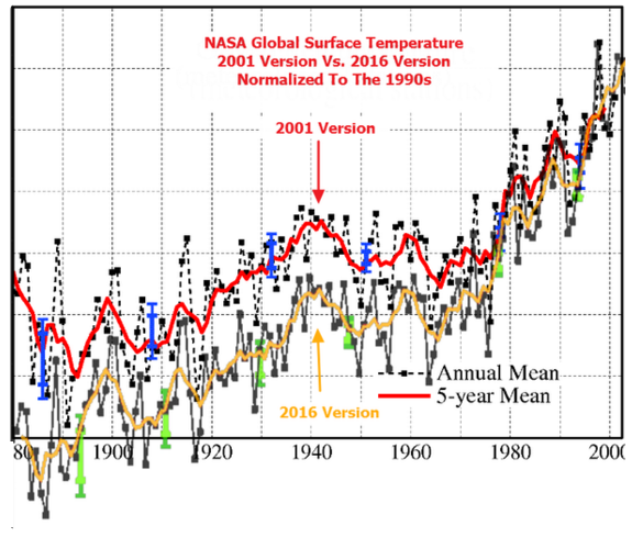
Notice that Mosher never gives any science, he just claims CO2 warms the planet. To hades with the ice core data that shows otherwise, and to hades with thermodynamics that says otherwise. And those poor scientists that worked in the space program who developed the “US Standard Atmosphere” — I bet they feel foolish for being so correct. After all, there is no mention of the back-radiation delusion at all.
Oh, and he takes a shot at a group in his number 1 that we can not even link to or mention by site policy. Perhaps Mosher will travel over and tell Dr. P*st** what he thinks.
“Notice that Mosher never gives any science”
Perhaps there’s a reason for that…
You neglect the fact that increased trees/plants/flowers/weeds that are growing INCREASE the absorption rate of CO2 from the atmosphere… !!
“Yes throw salby under the bus. You cannot on one hand demand that folks follow the scientific method, publish their data and code, and then let SALBY lead your charge”
Salby has far greater credentials than you do, Steven. Your bio says you were an English major. Why do you feel I should weight your scientific opinion more heavily than his?
I do not make it a habit of allowing people who are manifestly wrong about one thing dictate to me what I must accept as right about another.
In this case, the evidence is very clear – human inputs have little impact on atmospheric CO2 concentration.
All right – 4 years Bachelor’s in an engineering discipline, +2 years Master’s, +2 years PhD.
I think that holds up fairly strongly against an English major.
Steven’s bio, as ferreted out by sleuth Poptech:
http://www.populartechnology.net/2014/06/who-is-steven-mosher.html
That is a really dumb analogy.
All engineers study science. Few lawyers are heart valve engineers.
Any engineer has enough scientific education to evaluate CACA and find it ludicrously wanting. Few English majors and marketers are qualified to comment upon, let alone practice science.
Their credentials are irrelevant to my point, and has nothing to do with why your claim about civil engineers missed the mark.
I mentioned Mosher because he happens to have a poor understanding of statistics and repeatedly makes claims that reflect that. He gets some things right, but his scorecard is abysmal.
I also tire of the apparent lack of understanding of how feedback processes work by those untrained. The fact that Bartemis has to keep repeating the difference between a proportional relationship and an integral relationship could very well be related.
Or do you go only by grad and undergrad degrees, not considering work experience as a credential or qualification?
http://www.zoominfo.com/p/Rudyard-Istvan/27615932
As I said, an impressive and continuing career. Even his retirement farm brings science experience.
Why do refuse to open the link I showed you.
Rud’s career post-MBA and -JD is what matters. He had enough scientific education and on the job experience to contribute to the advancement of applied science in the 20th and 21st centuries, in different fields.
You, not so much.
The point of science is that one should be able to explain your evidence to anyone who has enough backround to follow the argument. The issue is more of having any understanding of any hard science field, and the attitude that gives towards using evidence. English Literature does not give that sort of “education”.
That is not to state that Eng Lit majors are irredeemable, only that any understanding of science is something they picked up outside their major field of study.
i was a psych major, and my evaluation of my math skills is that they suck. I can sorta follow math, but it is about as awkward as using a bilingual dictionary to translate. Getting the idea of sampling error and bias is something I do have a feel for, though. Psych does have a nasty tendency towards “cargo cult science” though, and the field is not quite “science” yet.
Since you can’t handle the truth and refuse even to look at it, I’ll save you trouble of clicking on the link:
http://www.mpr-inc.com
Rudyard IstvanRudyard IstvanRudyard L. Istvan is CEO of Third Stream Bioscience, Inc., a startup to commercialize a novel antimicrobial technology, and is also engaged in private equity investing in the energy, biotechnology, and semiconductor arenas.Rud was formerly EVP and a Director of GMP Companies, Inc., a privately held medical technologies company that among other things commercialized a wireless patient monitoring system based on Motorola patents.He joined GMP from Motorola, where he was a SVP, the Director of the Corporate Strategy Offices, and General Manager of Future Businesses.While at Motorola, Rud was involved in two major reorganizations, three acquisitions, several divestitures, and was the initial manager of new business platforms including Energy Systems, RFID/Smartcards, GMRAM spintronic memory, and Biochip Systems.Prior to joining Motorola, he was a SVP (senior partner) of The Boston Consulting Group heading two worldwide practice areas and the audit committee of the Board.He holds a summa cum laude in economics from Harvard College, a JD cum laude from Harvard Law School, and an MBA from Harvard Business School where he was a Baker Scholar.He captained Harvard’s 1971/72 national championship sailing team.He holds eight issued and several pending patents, has published a number of book chapters and articles in the energy and strategy arenas, and has been a director of several privately held corporations and charitable organizations.He is a member of the Massachusetts Bar.
http://www.gmpcompanies.com [cached]
Rudyard L. Istvan, J.D., M.B.A.Executive Vice President, Global Strategy Mr. Istvan is the Executive Vice President, Global Strategy for GMP Companies, Inc.He has also served as a member of the Board of Directors since the company’s inception in May 1999.Most recently, Mr. Istvan served as senior vice president and the general manager of Future Businesses for Motorola.He led Motorola’s creation of major new business platforms and headed their life sciences initiative which includes Motorola’s BioChip Systems and Clinical MicroSensors Divisions, the newest of their business platforms.Mr. Istvan also had worldwide responsibility for corporate strategy, venture investing and certain classes of technology out licensing.Prior to his tenure with Motorola, he spent 15 years with the Boston Consulting Group, and as Senior Vice President, headed two of their worldwide practice areas.Mr. Istvan is a member of the Massachusetts Bar and holds seven issued and several pending patents.
http://www.prnewswire.com [cached]
MOUNTAIN VIEW, Calif., Sept. 20 /PRNewswire / — Iconix Pharmaceuticals, a chemical genomics-based biotechnology company, today announced that Rudyard L. Istvan has joined the Company’s Board of Directors.Mr. Istvan’s participation comes as part of the recently announced partnership between Iconix and Motorola (NYSE : MOT) to enable the development of Iconix’s next generation chemical genomics database system, called ChemExpress (TM).Mr. Istvan brings to Iconix over twenty years of experience in new business creation, strategic planning and financing, and is a pioneer in the emerging convergence between the hi-technology and life sciences industries.He is a Senior Vice President of Motorola, Inc. and General Manager of Future Businesses.Mr. Istvan has worldwide responsibility for identifying and developing new business platforms, venture capital investing and licensing certain classes of technology to outside interests.He heads Motorola’s life sciences initiative, which includes Motorola’s BioChip Systems Division, and Clinical Microsensors, the newest of the new business platforms.Prior to joining Motorola in 1991, Mr. Istvan was a Senior Vice President of Boston Consulting Group.Mr. Istvan holds a B.A. summa cum laude in economics from Harvard College, a J.D. cum laude from Harvard Law School, and a M.B.A. from Harvard Business School where he was Baker Scholar.He is a member of the Massachusetts Bar, holds six U.S. patents and is the author of several publications.In addition to Iconix, Mr. Istvan sits on the boards of directors for Global Medical Products, Inc., Tissue Informatics, Inc., First International Digital Corp., and Hadley School for the Blind.
http://www.advancedautobat.com
Rudyard Istvan
NanoCarbon, LLC Rudyard Istvan Rud Istvan is the principal of and inventor behind NanoCarbons LLC. Since 2005 he has also been Chairman and CEO of Third Stream Bioscience, Inc., a private corporation commercializing an antimicrobial licensed from P&G. He was previously a senior vice president at Motorola and a senior partner at BCG. He holds a BA summa cum laude from Harvard, a JD from Harvard Law School, and an MBA from Harvard Business School. He holds 12 issued and 13 pending US patents in four subject areas, and has authored the ebooks Gaia’s Limits and The Arts of Truth.
http://www.zohshow.com [cached]
Over the next four or five years , we plan to develop and refine the technology to mass produce biochips , said Rudyard L. Istvan , Motorola vice president and corporate director of strategy.This should reduce their cost and make them widely available to genetic researchers in many fields..
The relevant quote was posted at 10:51 a.m.:
“The differential relationship indicates causality. It would be absurd to claim that the rate of change of CO2 is driving temperature – were that the case, CO2 could rise to arbitrarily high levels, but once it stopped rising, temperatures would fall back to their original level. Thus, it is temperature driving CO2, and not the reverse.”
more than 3 hours before your post at 1:54 p.m. in which you said:
” However, Bartemis confuses correlation with causation. His “relationship” is mere correlation, and he expounds it as causal.”
It is quite clear he is NOT confusing correlation and causation, and it is also quite clear you are not following his argument very well. Certainly not well enough to dismiss it in such a manner. Logic…
Again, irrelevant. You claimed he confused correlation with causation. He did not, and he offered a physical reason why. If you had instead argued that his reason for causation was poor, you’d at least not be wron due to a logic error. But you didnt, you made a completely incorrect claim. Logic…
Lest we forget, even Bill Nye has six semesters of calculus. Since the calculus curriculum is usually 3 or 4 semesters, I wonder which courses he had to repeat.
https://www.yahoo.com/tv/bill-nye-defends-science-guy-title-late-show-090328906.html
WRT Poptech.
Well I started as a Math Physics major in College.
Really wasnt challenging so I switched to Philosophy and English and Linguistics.
Double major in Philosophy English. Double honors. Phi Beta Kappa, blah blah blah
Grad school for English. My director was George Guffy ( formerly a geology student) and Vinton Deering
twp of the first guys to do computing in the humanities
My Phs did was on using information theory ( Shannon) to measure stylistic novelity or entropy if you like
This required that I go audit a bunch of stats courses, No problem since I enter school as a math major.
Any way a long the way my friends at Northrop recruited me to work in operations research.
1. Cause my work in grammar trees was applicable to markov series modelling of air combat
2. I could write
OR is basically modelling and when I was cleared into working on the F23 I was made director of OR
The cool thing was the instruction, because the stuff was all classified you could never have
learned it in school even if you wanted to. Plus there were great engineers who were stuck doing nothing
who would sit with me for hours and give me lessons, books homework, night classes to take
I mean there was NO TEXTBOOK on Lo observables.. the guy sitting next to you was one of 2 guys on the planet who knew how it worked, As for IR you’d get similar on the job training.
Build a radar model to simulate how an ESA radar works? Easy,, sit down with the engineers. get your lessons.. read the HUGHES radar book.. 12 hours a day 7 days a week, total fun. Build your simulation
test it.. go to the desert and strange places in nevada.. total fun. Brief the general.
It was a great learning exercise.. Boss brings you to a room. shows you silicon graphics.. says
Learn how to program these 3D computers, Its math so its easy. You take a few classes in silicon valley. Youre young nothing to do but learn and work. Nobody gives a rats ass if your a college boy or not.
And during all of this engineers still laughed and introduced their boss as the english major– who cant spell for shit.
recently switching back and forth between marketing and technical work ( mostly machine learning
for commercial customers ) has confused a bunch of people. Doesnt confuse me to be writing models one day and doing marketing the next day. Confuses other folks,, not me. Now add a hobby of doing data analysis for climate science,, and that really fries peoples minds.
I do however believe that Both Willis and Rud, trump me for being able to do wildly different things
I cannot fathom being a sailor or a lawyer.
Anyway, cool thing is now I get to go back to some of my roots and work again on AI. Mostly marketing, a little bit of product engineering.. The first design is done, next one ( I hope ) will do some things Ive always wanted to do in hardware. We will see.. probably wont happen till we go to 7nm.. company is worth 480M today ( just got 43M)
Maybe Rud wants in??
+ Bartemis said: “In this case, the evidence is very clear – human inputs have little impact on atmospheric CO2 concentration.”
Salby makes this case. He shows the rise of atmospheric CO2 concentration and the massive (and now dominant among human sources) CO2 emissions of China. They are not correlated. Human CO2 rates are not correlated with the steady CO2 rise since recordings began (presumably since the end of the Little Ice Age).
Salby may be wrong that his “surface properties” are not the cause of the CO2 rise, but be is absolutely correct that the observed CO2 rise is not correlated with massive changes in human CO2 emissions.
It is important people reading understand that if Salby’s alternative hypothesis for the CO2 is not correct then that does not mean that the IPCC’s AGW hypothesis with humans as the source of the CO2 is not necessarily correct either. Both can be wrong.
Sorry boys,
Credentials are of no interest here, only what people shows as understanding and reasoning in discussions.
I know that Bart is extremely good in frequency analysis and math, but lacks any insight in simple linear processes like many are present in nature. That makes that he concludes a lot from a nice match of noise in a graph and concludes that is causal, which is true, but then he goes on to declare that the trend is causal too, which is largely bogus, as it is easy to match two straight slopes which are not too different…
There are lots of problems with his theory:
1. His theory violates about all observations. Not one but all.
2. He compares the temperature trend with the trend of the derivative of CO2 (as Salby does too).
The causal relationship of the correlation – with a lag – between the variability (the noise!) is between T and CO2 and between dT/dt and dCO2/dt, not between T and dCO2/dt.
That there is a high correlation between all variabilities is because any sinusoid in its derivative remains the same sinusoid, only shifted pi/2 pack in time, so that T variability and dCO2/dt variability are largely synchronized. That means that there is no integral relationship between T and CO2 levels, the integral relationship is between dT/dt and CO2, where dT/dt has no trend and only a small offset:
http://www.ferdinand-engelbeen.be/klimaat/klim_img/temp_dco2_d13C_mlo.jpg
Which BTW proves that vegetation is the main reactant on the temperature variability, which can be seen in the opposite CO2 and δ13C changes. As vegetation is a net, increasing sink over time for CO2, it is NOT the cause of the trend, the trend is caused by a different process.
Rests human emissions at twice the increase in the atmosphere as cause of the trend, which is consistent with all observations…
See further about the origin of the CO2 increase:
http://www.ferdinand-engelbeen.be/klimaat/co2_origin.html
And about (spurious) correlations and causation of the same:
http://www.ferdinand-engelbeen.be/klimaat/co2_variability.html
MOA,
You have two variables, both influencing CO2 in the atmosphere:
– Human emissions with a huge trend and no measurable variability.
– Temperature with a small trend and huge variability.
Mix them together and you have some variability around a huge trend.
In the real world, only half the first remain in the atmosphere (as mass, not the original molecules), still some 80 ppmv since 1958. The temperature caused variability seems to be just noise of +/- 1.5 ppmv around the huge trend of 80 ppmv, here enlarged to show the extremes (Pinatubo, El Niño):
http://www.ferdinand-engelbeen.be/klimaat/klim_img/wft_trends_rss_1985-2000.jpg
All the correlation ánd causation is between total human emissions and total increase in the atmosphere, not between temperature and CO2, as the variability of temperature is not even visible in the trend of CO2:
http://www.ferdinand-engelbeen.be/klimaat/klim_img/temp_co2_acc_1960_cur.jpg
By looking at the derivatives, you just remove almost all of the trend, thus also the cause of the trend, while enhancing the noise…
Mosh has been at the AGW propaganda kool-aide.
3) the main warming out of the LIA was before 1920, so it is nothing to do with human CO2.
There has been little or no warming in the satellite era apart from the effects of El Ninos.
There is NO CO2 signature at all in the satellite era, despite that being when most human CO2 has been released.
Warming isn’t the threat.
A LIA 2.0, or even a mini-LIA of 30-50 years, would be catastrophic to mankind and ignite many wars, migrations in a grab for dwindling resources. And a desperate-for-food-and-energy 7 Billion people would do a tremendous amount of environmental damage to survive even a decade-long run of global crop failures due to freezing temps during growing seasons.
Until we understand the “why” of the LIA (causation), then more CO2 and more economic and infrastructure development are insurance against LIA 2.0. Wasting resources on inefficient solar and wind power, instead of nuclear power and infrastructure resilience, just makes guys like Elon Musk and Tom Steyer richer at humanity’s expense.
Joel,
If a Mini-Ice Age should occur in this century, then we will want to burn as much coal as possible, whether CO2 has any effect on air temperature or not.
But first the peasant will rise up and burn the crooked “climate science” charlatans whose voodoo sacrificed so many trillions in treasure and millions of lives. Tens or hundreds of millions in the case of even a little Little Ice Age.
+Joel O’Bryan wrote : “A LIA 2.0, or even a mini-LIA of 30-50 years, would be catastrophic to mankind and ignite many wars, migrations in a grab for dwindling resources. ”
I would not worry about heating or cooling. Anyone who reads and has understanding of what Koran 9:29 and hadith Sahih Muslim 6985 are talking about should be focused there. ‘Climate Change’ of a LIA is nothing in comparison to the coming Demographic Change.
We are about to start our lessons in practical LIA studies in mid-America. Eurasia started last September, but who would notice. The snowflakes may get hungry after a while, then the noise will start. They’ll need their pussy hats.
Thanks, Mosher. I agree fully (for once) with your comment, which is why I bothered to resurrect this and spiff it up yesterday after the OCO-2 comments. IMO it does skeptics general harm (presidential label as flat earthers) not to reject ALL incorrect arguments no matter how they cut, which includes projecting more certainty than justified by circumstances.
This is now the third time since the 2015 London video that Salby has been a post topic here. I just spent time skimming all the comments on the previous two. Found two things. 1. Lots of coupled beliefs in junk science; Salby is right and Gold (abiotic oil) is right. 2. Some WUWT skeptics really aren’t. They have D***** beliefs that do not change in the face of new solid evidence.
To that group, I urge considering John Maynard Keynes (paraphrased) response to new (theory refutation) evidence: ‘I change my mind. What do you do?’
Thanks Rud.
At the core there is much we agree about.
Accept my apologies for flame wars on the minor points where we do not agree
+ristvan – Salby’s alternative hypothesis as “surface properties” (which could be flora or, more likely, microbial fauna) as the cause of the increase in CO2 could well be wrong.
However, Salby’s main point was to compare the rate of human emission of CO2, now dominated by a massive increase from China, yet the rise of CO2 concentration in the atmosphere is not correlated at all with changes in total human emissions.
Salby could be wrong about the apparently natural mechanism, but he appears to be right that humans are not the source of the CO2 rise – since changes in human CO2 emissions are not correlated at all with the observed atmospheric CO2 concentration rate-of-change.
I just want readers to understand since Salby may have got the mechanism wrong it does not mean that human-emitted CO2 must be the cause. Both Salby and the IPCC can be perfectly wrong on this.
MOA,
The correlation between human emissions and increase in the atmosphere is extremely good:
http://www.ferdinand-engelbeen.be/klimaat/klim_img/acc_co2_1960_cur.jpg
The increasing lag of the South Pole shows that the main source is in the NH. The same for the drop in δ13C, all caused by fossil fuel use.
By looking at the derivatives, Salby removed most of the trends and thus most of the cause of the trends, leaving the enhanced noise, which is only +/- 1.5 ppmv around the trend, while human emissions are +4.5 ppmv/year, each year again, leading to +2.15 ppmv/year, each year again…
“The correlation between human emissions and increase in the atmosphere is extremely good:”
The correlation between temperature anomaly and the increase in the atmosphere is better.
http://i1136.photobucket.com/albums/n488/Bartemis/tempco2_zps55644e9e.jpg
Rud – have you debated all this with Murry? Could be helpful.
It took some effort to go through the video many times until I could get it. In other words, I started off sceptical and ignorant of a new idea. I’m now willing to give it a chance as I continue my research and try to develope practical tests. Your refutation hasn’t convinced me at 1st look, but neither did Murry’s. Situation normal…..
Bart:
The correlation between temperature anomaly and the increase in the atmosphere is better.
R^2?
Moreover, it is very easy to match two straight lines (with the same added noise), far less easy to match two curvatories…
“…far less easy to match two curvatories…”
This is a plot of absolute CO2 versus the integrated temperature. As such, the individual variables independently do have significant curvature. It does not show up here because the curvatures are approximately the same, so it does not show up in a plot of the one against the other.
I think that most of us here will agree with you on these points. The disagreements here are the details.
Sorry. Out of place. I came back from an errand.
Mosher –
I’ve been hanging around on WUWT for a few years now, and your post on May 13 at 10:37am is one of your better, if not best, ones regarding the general CAGW discussion.
However, your “Three Questions” aren’t complete:
1. How much will we emit in the future? Assuming in this discussion you mean CO2 emissions, this is a reasonable question only if it can be shown definitively that our CO2 emissions are having a noticeable or measurable effect on the temperature of the atmosphere.
2. How much will we warm? Better perhaps would be “How much will the atmospheric temperature change? It could cool or the “pause” could be longer term or, of course, some additional warming could occur. Warming is not a certainty.
3. Should we and can we do anything? Assuming again that you mean regarding human CO2 emissions, this question is not really necessary to ask scientifically or politically unless it is a certainty that human CO2 emissions are having a noticeable or measurable effect on the temperature of the atmosphere.
So, before your three questions are worth asking, we must first ask the real, primary questions:
“What effect are human CO2 emissions having on the atmospheric temperature?
“What effect are human CO2 emissions having on the environment other than the possible effect on atmospheric temperature?”
Well said, JohnWho.
The lack of those two questions in Mosher’s post was also evident to me. But that is why Mosher is a believer. He doesn’t ask the right questions.
Furthermore, the rate of change of CO2 concentration is fairly constant. Meanwhile the rate of CO2 emissions from humans (now dominated by China) varies greatly. This was one of Salby’s main points, that the rise in atmospheric concentration is not correlated with the rate of human emission. There is something else at work and Salby posited “surface properties” as the correlated factor.
For those that have not seen Sa;by’s videos, he show China’s emissions go up by a factor of 3 to dominate human emissions, while those of Europe and the US start to drop. Meanwhile, the atmospheric CO2 concentration continues up at its steady rate – not correlated with large changes in human emission.
Thus, even if Salby is wrong about “surface properties” as being the source of the CO2, he is right that the rate of change is not directly correlated with human emissions. The IPCC’s AGW hypothesis remains wrong.
JohnWho writes
And if there is a noticeable effect we must establish whether the net effect of additional CO2 is for the better or worse. There seems to be an unquestioned assumption that any additional CO2 and warming will be bad for the planet even though the warming so far would seem to have been good.
Moa,
You have it upside down: human emissions show little variability and a huge trend (a fourfold increase since 1958), while temperature is the main driver of the variability.
That makes that the huge correlation is with temperature in the derivatives, but that says next to nothing about the cause of the trends, which are largely human…
MOA, read Willis’ post. The atmospheric CO2 concentration is NOT a function of annual emmissions. It is a function of cumulative emissions. That greatly damps the recent impact of China. Thendistinction between annual and cumulative is one of the Salby definitional flaws.
Seems to me there is a question that underlies both those questions;
When we will have sufficient means to know what effect human CO2 emissions are having?
Climate science is so immature and the processes so complex it doesn’t appear to me that we yet know how to go about answering those questions let alone actually answering them.
“You cannot on one hand demand that folks follow the scientific method . .. ”
You are joking right? When has Climate Science ever adhered to the Scientific Method?
The Climategate emails clearly showed this is/was a political movement — dodging FOIA requests, deleting emails and data, conspiring to blackball legitimate scientists, and corrupting the peer-review process was never apart of true science.
@ Steven Mosher May 13, 2017 at 10:37 am
Steve Mosher seems to be addressing science dummies like me:
#1 C02 is a GHG.
Yes I get that.
#2 Humans are responsive for the rise in C02.
There seems to be a causality dilemma aka ‘chicken and egg’ problem vis-à-vis CO2 and temperature, the causality can go in either direction and I don’t mean in the feedback sense, it doesn’t have to be one thing or the other but a combination of factors.
The LIA was about the coldest this interglacial has been and although the idea is scoffed at by alarmists, a natural ’recovery’ component is entirely consistent with the paleo. record.
#3 The world is in fact warming.
Fortunately it is, the accurate degree is sadly unknown due to the disgraceful behaviour of agenda-driven surface temperature collectors and curators.
#4 If my bank balance didn’t go up consistent with a constant income flow I’d want to know why.
The IPCC claims that CO2 is the overwhelming temperature forcing factor overriding all other factors.
Mosher makes 4 points. They probably match up with what ExxonMobil is saying. Why would that corporation say these things? They’re smart.
Poptech has an ax to grind. It highlights marketing a number of times. Marketing is important. If something doesn’t sell, I am sorry, it was a hell of an idea, it lost money. The product should have a certain level of quality. To have that quality at a blog, there should be adversarial discussion not only directed at the warmists who don’t show up.
This acceptance of what is unreasonable yet on our side might be left to the warmists. We’ve made calls for them to reign in the nonsense when they see it.
Mosher, I agree with the exception of the “real question” of “how much will we warm.” The experiment (adding CO2) has run long enough for use to reach a conclusion. There is no evidence that warming over the next, say, 100 years will be any worse than the warming over the past 100 years—current models are not evidence)—and the warming over the past 100 years has led to global average temperature increase that could not be sensed by the average human if it occurred over a period of seconds. There has been no increase in the rate of sea level rise and no increase in dangerous weather. The world is slightly warmer, slightly wetter, and much greener. No cause for alarm and certainly no justification for expensive fixes.
“1. C02 is a GHG.”
Yes Steven, you need to dive a little deeper than your high school physics. Perhaps a little correct speak will help. CO2 is a “challenged” greenhouse gas.
“2. Humans are responsive for the rise in C02.”
I make typos too, and you may be right; but this statement is by no means as certain as you suggest.
“3. The world is in fact warming.”
Since the LIA no doubt. Steven, did a sudden drop in C02 cause the LIA?
“4.”
Not even wrong, except for the final three questions. YOU, are the flat earther, if you refuse to even consider alternative explanations for your three epistles above.
GHGs distribute heat; do they make it warmer: how does the average Moon temp cf Earth’s: 243K:286K
At the very least you could get the formula for carbon dioxide right. It’s CO2.
Perhaps someone can explain this better for me. I thought “the pause” was based on the temperature anomaly. That being said, the anomaly is based on the normal warming rate since emerging from the last ice age (or little ice age). The normal warming rate “x,” plus the increased warming due to AGW “y” (anomaly) is in theory the total rate of warming. So even if there is a pause in the anomaly, do we not still have a base warming rate causing increased CO2 degassing?
The pause was an actual pause and not a pause in the increase in warming. The overall trend over 19+ years was zero. The recent El Nino increased that trend line but the trend line is quickly creeping back toward zero with the current, post El Nino, cooling.
AM, misdefinition of anomaly. Because different latitudes and altitudes have different temperatures, they cannot be directly compared. So for each place (say a GHCN station, a thirtynyear average is computed, say from 1980-2010. Then the anamoly is just the difference from the baseline. That way, global temperature anomalies have meaning as everywhere comparable trends. The baseline includes both natural warming since the LIA and any AGW, as does the anomaly. Sorting between natural and AGW trend causes is the attribution problem.
1980-2010,,,,
I know that was just an example….but it did make me chuckle a little
It also depends on where the pick that 30 year period……if they had picked 1940-1970 it would be completely different
Got me there. But a couple of more serious observations. 1. For trends, itmdoes not matter which 30 year period is chosen. Absolute Anomalies will differ, but not their trends. 2. Where anaomalies become perniciousmis in hiding climate model fails. Did you know thatnon a real temperature basis CMIP5 varies by +/- 3C, so none get water phase changes ‘right’? Essay Models all the way Down reproduces the figure from the comparison paper. Not something you will ever see in an IPCC document.
…bingo!
FTA:
“First, if Salby is right, the rise in atmospheric CO2 concentrations should have slowed or stopped because of the ‘pause’. They haven’t.”
This shows that Rud has not followed the argument in the slightest. Salby’s model says that there is an integral relationship between temperature anomaly and atmospheric CO2. That is, the rate of change tracks temperature to high fidelity according to the differential equation
dCO2/dt = k*(T – T0)
CO2 = atmospheric CO2 concentration
T = temperaure anomaly
T0 = equilibrium temperature
k = coupling factor in ppmv/degC/unit-of-time
As long at T remains above T0, CO2 will continue to accumulate.
The relationship holds reasonably well with respect to the long term surface data record:
http://woodfortrees.org/plot/esrl-co2/derivative/mean:24/plot/hadsst3sh/scale:0.23/offset:0.103/from:1960
and holds even better with the more accurate satellite data in the era since they came online:
http://woodfortrees.org/plot/esrl-co2/derivative/mean:12/from:1979/plot/uah6/offset:0.73/scale:0.2
Integrating the relationship shows that there is an excellent match with overall change in concentration:
http://woodfortrees.org/plot/esrl-co2/derivative/mean:24/integral/plot/hadsst3sh/scale:0.23/offset:0.103/from:1960/integral
Human emissions need not apply. They are superfluous. All one needs to predict the level of CO2 in the future is the temperature record.
The differential relationship indicates causality. It would be absurd to claim that the rate of change of CO2 is driving temperature – were that the case, CO2 could rise to arbitrarily high levels, but once it stopped rising, temperatures would fall back to their original level. Thus, it is temperature driving CO2, and not the reverse.
Moreover, the relationship indicates that temperature sensitivity to CO2 is negligible. Were it not, a positive sensitivity would produce an unstabilizable positive feedback, and we would have reached a saturation state eons ago.
“Second, satellites have NOT generally observed higher CO2 concentrations over uninhabited/ unindustrialized regions in past two decades.”
Has no bearing on the validity of the model. The plots above demonstrate that the model holds to high fidelity.
“That is NOT true either; both land and sea have been serving as net sinks.”
That is not so. These are only assertions, and they are tripping very close to the widely debunked and absurdly idiotic pseudo-mass balance argument.
I explain the problem with the pseudo-mass balance argument here. I provide a model for how the oceans can produce the observed integral relationship here.
“First, if Salby is right, the rise in atmospheric CO2 concentrations should have slowed or stopped because of the ‘pause’. They haven’t.””
A saucepan will continue to simmer even when the heat is turned down.
And ice continues to melt once it is warm enough.
2017: Slowest “melt from maximum” in MASIE. Not much melting happening.
MASIE has sea ice now above all year since 2006 except 2012, 2013
AndyG55 on May 13, 2017 at 1:56 pm
2017: Slowest “melt from maximum” in MASIE. Not much melting happening.
We are completely out of topic in this heavy discussion about CO2, but as usual, AndyG55 manages to present us a small piece of a picture as if it was the whole.
Here is a plot of all monthly Arctic sea ice extent departures from the climatology (1981-2010) since january 1979:
http://fs5.directupload.net/images/170516/5ff68zxl.jpg
Do you see the rightmost orange drop, AndyG55?
That is what you show us…
1. What about looking at what happened in the few years before?
2. How many time will the planet need, do you think, to recover from the level at the right of the plot to the level at its left?
To conclude, let me do the same kind of cherry picking as you did, by now displaying the daily data from April, 1 till May, 14:
http://fs5.directupload.net/images/170516/a6h57h67.jpg
Do you understand what I mean, AndyG55?
Source: ftp://sidads.colorado.edu/DATASETS/NOAA/G02135/north/daily/data/
both land and sea have been serving as net sinks….
A more correct description would be like a bank……where you make deposits and withdrawals
…and exactly like a bank…withdrawals happen faster than deposits
Thanks for reproducing that math, Bartemis. Now respond using your Salby math to the first posted example figure in the critique section of the guest essay, charted data concerning the post 2000 temperature pause and CO2. Nevermind what should have happened to the Keeling curve 2015-16 if Salby is correct (cause it isn’t in that figure– but the data exists). And please go back to the videos to also verify Salby’s mathematically derived source response lag time was on order of 10 months IIRC. So the 2015-16 El Nino spike gives another empirical observational test of Salby’s theory. I was just too lazy to add it. Once a theory is disproven, more disproofs do not make it deader or wronger. One suffices.
FAIL.
No, Rud. You still do not understand the model. It fits quite well with the latest El Nino.
http://i1136.photobucket.com/albums/n488/Bartemis/CO2intgtemp_zpstgwfvicg.png
Crickets.
I am beginning to believe that Rud does not know what an integral is.
Salby’s view of CO2 in the pre-OCO-2 era was informed by NASA’s now debunked 2006 model for global CO2.


This NASA CO2 model is now understood as based on falsified assumptions.
http://www.euanmearns.com/wp-content/uploads/2015/01/1_dec_06.png
OCO-2 will eventually revolutionize the scientific understanding of where the structural regional sinks and sources are located and their kinetics. The seasonal data is so noisy and varying. It will take at least several more years of data collection and seasonal integration to deconvolve what are the natural regional structural sources and sinks and what ones are transitory or on-off sources/sinks such as volcanic/tectonic short term releases.
I have watched the latest OCO-2 video several times, and I find it somewhat misleading by trying to create a 3D type view by looking northward from the southern hemisphere (sort of like trying to peek under a dress).
An across seasons OCO-2 snapshots.
NH winter / SH summer – (late January to early February) 2015
NH summer/SH winter – 2nd half of July 2015
What will help immensely with the OCO-2 snapshots is a detrending of the secular [CO2] rise of ~2.5 ppm/yr so that visualization across about 4-5 years of data can be seen without the changing CO2 baseline color scale.
For example – because of the secular global rise of ~3 ppm between 2015 to 2016 (driven higher by El Nino),
trying to visually compare the first two weeks of June 2015 with the same period in June 2016 is difficult.
1st two weeks of June 2015
1st two weeks of June 2016
Detrending the CO2 secular rise would allow a better visualization of where the structural sources and sinks are operating.
OCO-2 annualized visualization, which factors out seasonal effects (from Eric Swenson, posted originally here
Picking cherries.

http://i59.tinypic.com/vy1p2c.png
Rud – you have fundamentally misapprehended Salby’s argument and his model. You are not even wrong. You are just off beating a straw man of your own construction.
Bartemis, I totally agree. Sad, and I don’t hear yet if Rud has corresponded with Murry, and if so what transpired. The proponent needs to get a hearing, not just Rud. Salby does have a basis in physics for his arguments. As he should. CO2 levels, poorly defined at best, in spite of silly modeled red clouds from Nasa, march to a different drummer……As Murry claims.
However, thanks Rud, this is a start.
Salby’s view of CO2 in the pre-OCO-2 era was informed by NASA’s now debunked 2006 model for global CO2.


This NASA CO2 model is now understood as based on falsified assumptions.
http://www.euanmearns.com/wp-content/uploads/2015/01/1_dec_06.png
OCO-2 will eventually revolutionize the scientific understanding of where the structural regional sinks and sources are located and their kinetics. The seasonal data is so noisy and varying. It will take at least several more years of data collection and seasonal integration to deconvolve what are the natural regional structural sources and sinks and what ones are transitory or on-off sources/sinks such as volcanic/tectonic short term releases.
I have watched the latest OCO-2 video several times, and I find it somewhat misleading by trying to create a 3D type view by looking northward from the southern hemisphere (sort of like trying to peek under a dress).
An across seasons OCO-2 snapshots.
NH winter / SH summer – (late January to early February) 2015
NH summer/SH winter – 2nd half of July 2015
What will help immensely with the OCO-2 snapshots is a detrending of the secular [CO2] rise of ~2.5 ppm/yr so that visualization across about 4-5 years of data can be seen without the changing CO2 baseline color scale.
For example – because of the secular global rise of ~3 ppm between 2015 to 2016 (driven higher by El Nino),
trying to visually compare the first two weeks of June 2015 with the same period in June 2016 is difficult.
1st two weeks of June 2015
1st two weeks of June 2016
Detrending the CO2 secular rise would allow a better visualization of where the structural sources and sinks are operating.
…And that matters …why ?
Mr. Istvan breezily waves aside all the physics and data backing up Dr. Salby’s arguments with: There are fundamental definitional, mathematical, and factual observation errors. Given the expertise of Dr. Salby versus Mr. Istvan, here, this is laughable.
What is not laughable is Istvan’s ignorance (I will not accuse him of intentionally mischaracterizing Salby – I’ll assume Istvan simply did not know) of Salby’s actual arguments.
1.Istvan:
Comment: This is inaccurate. Salby discusses C12 versus C13 at great length, evidence for human emissions being overwhelmed by natural emissions. Further, while it is a key fact, Salby does not rely solely on the 2 orders of magnitude difference between natural and human CO2; Salby made it clear that the properties of C, and of CO2 and of the natural sources and sinks (e.g., oceans and forests) are highly significant.
2. Istvan:
Comment: This gross over-simplification shows that Istvan either did not read or has forgotten what he read (or heard). Salby did not “deduce.” Salby used ice core data analysis with damping equations to compute CO2’s lagging temperarature by a quarter cycle. Mischaracterizing Salby’s carefully calculated conclusions as a breathless, there must be, is silly.
3. Istvan:
Comment: From this inaccuracy, it is clear that Istvan has either forgotten or never carefully watched (or read) Dr. Salby’s Hamburg (2013) lecture in which he clearly states several times that CO2 lags temperature over a wide range of time scales. By stating the 800-year fact, etc., Istvan is apparently attempting to create the misimpression that Salby was not aware of these things.
4. Istvan:
Comment: Istvan provides exactly zero proof that OCO-2 “disproves” the SCIAMACHY (described here: https://earth.esa.int/web/guest/missions/esa-operational-eo-missions/envisat/instruments/sciamachy ) data.
5. Istvan:
Comment: Given what Salby actually argues, that CO2 lags temperature by a quarter cycle, the CO2 decrease is yet to materialize. Istvan’s mistake here is thinking that there is almost no lag at all.
6. Istvan:
Comment: LOL – prove it.
7. Istvan:
Comment: Simply incorrect.
http://ecco2.jpl.nasa.gov/menemenlis/articles/co2_source-sink_pp.pdf
8. Istvan:
Comment: In other words, “If I’m right, then Salby is wrong. Trust me. I know.”
I strongly urge anyone wondering if, after all, Mr. Istvan may have a point, to watch Murry Salby’s lecture. Let the man speak for himself.
(youtube – in English, only introduction is in German)
Janice, if you want a separate post to shred him in gory detail, you can get one. Eschenbach’s 2015 post made a fine start, and I provided the link. Willis did not finish simply because what he found was already so awful that he stopped. Go read it.
What part of a Feynman test do you not like? Salby reaches a wrong conclusion by confounding annual with cumulative, by confounding residence time with efold time, and by presenting ‘data’ that isn’t, which he claims cannot back up because his stuff remained at Mcquarie. I showed his Hamburg lecture CO2 land mass ‘data’ . Then showed that chart is simply bad data.
But the Feynman test is simple. Salby has a theory that rising CO2 mostly isn’t anthropogenic. So must be natural. If there are no net natural sources, then Salby is wrong without all the bother of explaining why in detail.
If you bother to dig into his Hamburg lecture, you will indeed find definitional problems. I mention in this comment the two highlighted by Willis at his linkd post aboutbthe London lecture. You will find mathematical errors. And you will find bad data, an indelible example of which is in the post based on the Hamburg lecture.
Please don’t give skeptics a bad name by carrying on so.
Salby is wrong. Get over it.
ristvan @ May 13, 2017 at 11:26 am
“If there are no net natural sources, then Salby is wrong without all the bother of explaining why in detail.”
You do not know the net natural sources. I think you have fallen prey to the mind boggling stupid pseudo-mass balance argument.
“Salby is wrong. Get over it.”
Exactly what are your credentials, Rud? If I recall correctly, you are not technically trained. Autodidacticism is all well and good, but you should be wary of presuming that other objectively highly skilled persons are wrong based on your misapprehension of their arguments.
Bart,
There are no huge, fast natural CO2 sources. It is that simple. Nothing to do with the mass balance (which fortifies that conclusion), but with observations.
– The oceans as total surface, including the upwelling and sink places is a net sink for CO2 based on 3 million CO2 samples over the past decades to centuries.
– The biospere is a net sink for CO2, based on the oxygen balance and satellite measurements of photosynthesis. The earth is greening.
Thus if you have no other fast, huge sources supporting your theory, then your theory is refuted by these observations.
“There are no huge, fast natural CO2 sources.”
Yes, there are. Every second of every day, CO2 laden waters are upwelling in the tropics.
“– The biospere is a net sink for CO2, based on the oxygen balance and satellite measurements of photosynthesis.”
Stupid pseudo-mass balance argument.
Ferdinand, did it ever occur to you that the ocean is a net sink for co2 because the mass of the anthropogenic source is equilibrium sinking into it?
Bart,
I know that you ignore any scientific evidence that even remotely threatens your theory.
The oceans are a proven sink for CO2, as every parcel of water coming up every moment of the day in the tropics is compensated by a similar parcel of water sinking near the poles. The net measured effect is that more CO2 sinks with the waters than is released by the upwelling.
The net effect in the rest of the ocean surface is an increase of DIC following (not leading) the increase in the atmosphere.
And an oxygen balance shows how much CO2 the biosphere sinks or releases, not stupid, neither a full mass balance, except if you find another source of oxygen in nature… Confirmed by the greening of the earth (or is that also a stupid mass balance?)
Fonzie:
Ferdinand, did it ever occur to you that the ocean is a net sink for co2 because the mass of the anthropogenic source is equilibrium sinking into it?
The oceans don’t react on human emissions of one year, they react on the total CO2 pressure in the atmosphere above (dynamic) equilibrium, no matter the origin of that extra CO2 or the CO2 composition (human/natural) of that moment.
For the current average ocean temperature the equilibrium is at 290 ppmv. We are at 400 ppmv. The extra 110 ppmv is what pushes more CO2 into the oceans and vegetation. That is net about 2.15 ppmv/year, or an e-fold decay rate of ~51 years. Not enough to remove all human emissions (as mass, not the original molecules) in the same year as released.
Well done, Janice.
Mod – my longer response to Rud’s post seems to have gone missing. Can you please see if you can find it? I would hate to type it all over again.
i’ve learned the hard way always to copy before hitting “Post Comment”.
Oh, Bartemis, thank you, SO much for that. Your technically highly skilled opinion weighs heavily with me. SO glad you took the time to educate us so ably here! Perhaps fchaynie and Allan M. R. MacRae (and others who have ably argued the facts on WUWT about CO2 lagging temperature will also show up).
btw: I think your detailed response finally appeared, here: https://wattsupwiththat.com/2017/05/13/is-murry-salby-right/#comment-2501545
Thank you Janice!
A very concise yet well constructed defence of Prof. Salby. It seems to me, in my limited knowledge of this debate that the question of CO2/temperature lead lag is highly significant. Whether the lag is months or centuries, if it exists, it matters. I have read some arguments denying the 800 year lag but they appeared weak and contrived compared to the evidence that it does exist.
The only potential explanation I can see for this relationship is outgassing from warming ocean waters. If such temperature dependent outgassing occurs, it must occur at the surface “skin” of the ocean as a result of vapour pressure balances. The amount of CO2 delivered to the atmosphere would be dependent on the rate of transfer to the surface from below, where temperature rise would be slower. I wonder if this might explain the time lag?
My own pet theory,but regardless I am loathe to see non standard ideas abused recklessly when the absolute garbage that passes for mainstream climate science is allowed to walk the earth without shame.
Aw, Mr. Harmsworth. Thank you. I realize that my arguments are surface level only. Glad they were helpful to you.
Your “pet theory” sounds plausible! 🙂
Mr. Harmsworth, you may find Dr. Salby’s July 18, 2016 lecture at University College, London helpful.
At ~ 44:00 he talks about “as the frequency {in temperature change} is increased, the lag is increased”
(youtube)
Just wanted to give you a possible place to look for equations which might support your “pet theory.”
@Bartemis: You might find Dr. Salby’s lecture above interesting (though you already know most (all?) of what he says there). Lots of equations!
@ Anyone wanting to learn! Watch the above lecture! 🙂
Very well done, Janice.
That was a fabulous take-down of the mischaracterizations tossed about here.
🙂
Thank you again Janice Moore.
The following was posted on Friday 12May2017 in an earlier article – as usual, those who responded did not bother to read what I wrote before they posted their replies.
For the record, I disapprove of the rancor that is so often displayed in this discussion – Murry Salby is a decent guy who has been severely wronged – the “piling on” against him is bullying.
At the risk of offending both sides of this SCIENTIFIC argument, I am agnostic about it. As I stated below:
“While this question is scientifically interesting, it is not critical to the assessment of the risks of catastrophic humanmade global warming (“CAGW”). One can make conclusions regarding the risks of CAGW with a high degree of confidence, without fully resolving the primary source of increasing atmospheric CO2.”
Consider the following hypothesis:
“Something” is causing an increase in atmospheric CO2 – this CO2 increase could be mostly natural or mostly humanmade. On top of this CO2 increase is a clear signal, that CO2 lags temperature by ~9 months in the modern data record. The causative relationship dCO2/dt vs. temperature T is incontrovertible.
http://www.woodfortrees.org/plot/esrl-co2/from:1979/mean:12/derivative/plot/uah5/from:1979/scale:0.22/offset:0.14
CO2 also lags temperature by ~~800 years in the ice core record. CO2 lags temperature at all measured time scales.
I suggest that the following conclusions are valid:
TEMPERATURE, AT ALL MEASURED TIME SCALES, DRIVES CO2 MUCH MORE THAN CO2 DRIVES TEMPERATURE.
What we see in the modern data record is the Net Effect = (ECO2S minus ECS). I suspect that we have enough information to make a rational estimate to bound these numbers, and ECS must be very low, so small as to be practically insignificant, far too small for there to be a significant risk of dangerous humanmade global warming.
Regards to all, Allan
https://wattsupwiththat.com/2017/05/12/surprising-nasas-global-visualization-in-3d-of-carbon-dioxide-in-earths-atmosphere/comment-page-1/#comment-2501415
Thank you Janice Moore for your kind words above.
For clarity, I do not necessarily suggest all or even most the observed increase in atmospheric CO2 is natural – like my friend Richard Courtney I am more of an agnostic on this subject. While this question is scientifically interesting, it is not critical to the assessment of the risks of catastrophic humanmade global warming (“CAGW”). One can make conclusions regarding the risks of CAGW with a high degree of confidence, without fully resolving the primary source of increasing atmospheric CO2.
It is incontrovertible that annual atmospheric CO2 flux (the Keeling curve) is dominated by natural seasonal temperatures – the cause of this seasonal flux is overwhelmingly natural and temperature-driven. It is also incontrovertible that atmospheric CO2 lags (in time) atmospheric temperature at all measured time scales (MacRae 2008, Humlum 2013 and others).
Since I wrote that conclusion in 2008, few climate scientists have wanted to even acknowledge this incontrovertible fact. To this day, the mainstream debate between climate skeptics and global warming activists continues to concern the sensitivity of climate to temperature (“ECS”) – or by how much the future can cause the past. 🙂
The following post attempted to focus the debate on what really matters – that based on the evidence, ECS is so small as to be insignificant, and the risks of CAGW are also similarly so.
Regards, Allan
https://wattsupwiththat.com/2017/04/12/perspective-needed-time-to-identify-variations-in-natural-climate-data-that-exceed-the-claimed-human-co2-warming-effect/comment-page-1/#comment-2477211
Excerpts from the following post:
All that really matters [in this analysis] is that CO2 lags temperature at ALL measured times scales and does not lead it, which is what I understand the modern data records indicate on the multi-decadal time scale and the ice core records indicate on a much longer time scale.
…
It also does not mean that increasing atmospheric CO2 has no impact on global temperature; rather it means that this impact is quite small.
…
What we see in the modern data record is the Net Effect = (ECO2S minus ECS). I suspect that we have enough information to make a rational estimate to bound these numbers, and ECS will be very low. My guess is that ECS is so small as to be practically insignificant.
Regards, Allan
Please excuse the pedantic nature of the following treatise – I am so often misquoted on this subject that I tried to make it very clear where I stand.
https://wattsupwiththat.com/2017/01/24/apocalypse-cancelled-sorry-no-ticket-refunds/comment-page-1/#comment-2406538
[excerpts]
I have stated since January 2008 that:
“Atmospheric CO2 lags temperature by ~9 months in the modern data record and also by ~~800 years in the ice core record, on a longer time scale.”
{In my shorthand, ~ means approximately and ~~ means very approximately, or ~squared).
It is possible that the causative mechanisms for this “TemperatureLead-CO2Lag” relationship are largely similar or largely different, although I suspect that both physical processes (ocean solution/exsolution) and biological processes (photosynthesis/decay and other biological processes) play a greater or lesser role at different time scales.
All that really matters is that CO2 lags temperature at ALL measured times scales and does not lead it, which is what I understand the modern data records indicate on the multi-decadal time scale and the ice core records indicate on a much longer time scale.
This does NOT mean that temperature is the only (or even the primary) driver of increasing atmospheric CO2. Other drivers of CO2 could include deforestation, fossil fuel combustion, etc. but that does not matter for this analysis, because the ONLY signal that is apparent in the data is the LAG of CO2 after temperature.
It also does not mean that increasing atmospheric CO2 has no impact on global temperature; rather it means that this impact is quite small.
I conclude that temperature, at ALL measured time scales, drives CO2 much more than CO2 drives temperature.
Precedence studies are commonly employed in other fields, including science, technology and economics.
Does climate sensitivity to increasing atmospheric CO2 (“ECS” and similar parameters) actually exist in reality, and if so, how can we estimate it? The problem as I see it is that precedence analyses prove that CO2 LAGS temperature at all measured time scales*. Therefore, the impact of CO2 changes on Earth temperature (ECS) is LESS THAN the impact of temperature change on CO2 (ECO2S).
What we see in the modern data record is the Net Effect = (ECO2S minus ECS). I suspect that we have enough information to make a rational estimate to bound these numbers, and ECS will be very low. My guess is that ECS is so small as to be practically insignificant.
Regards, Allan
*References:
1. MacRae, 2008
http://icecap.us/images/uploads/CO2vsTMacRae.pdf
Fig. 1
https://www.facebook.com/photo.php?fbid=1200189820058578&set=a.1012901982120697.1073741826.100002027142240&type=3&theater
Fig. 3
https://www.facebook.com/photo.php?fbid=1200190153391878&set=a.1012901982120697.1073741826.100002027142240&type=3&theater
2. http://www.woodfortrees.org/plot/esrl-co2/from:1979/mean:12/derivative/plot/uah5/from:1979/scale:0.22/offset:0.14
3. Humlum et al, January 2013
http://www.sciencedirect.com/science/article/pii/S0921818112001658
I agree with you Janice.
I’d like to see some proper kinetic analysis of fluxes between various sinks/sources with characterisation before saying that Salby’s analysis is wrong.
As for quoting Eschenbach as an authority ……
Salby believes that the ice core record is not accurate to nearly the extent that is believed, when used to determine the CO2 in a given time range. He believes it is more a moving average of CO2. This means there could be periods of larges swings in CO2, like now, that are not reflected in the ice core records. I think that is probably closer to reality than some postings here subtracting 800 years and expecting CO2 to increase or decrease because to temperature from 1217.
Bill,
The resolution (indeed a “moving average”) of the ice cores depends of the local snow accumulation rate and is between 10 and 560 years. The current increase of 110 ppmv in 165 years would be visible in every ice core in the past 800,000 years, be it with a lower amplitude. The CO2 levels of ~800 years ago were around 280 ppmv with a resolution of ~20 years, not able to move current CO2 levels up to over 400 ppmv…
That’s because the CACA Team (their term) are the new Inquisition.
Interesting dispute, Rud, and a fair exposition on a theory.
TH, knew this would bring out Janice and Bartemis. Let others judge the outcome following Feynman’s rule. My job is done, as promised in the OCO-2 post comments.
Your job is woefully inadequate. You are not even arguing against Salby, but over some figment of your imagination.
Salby’s model posits an integral relationship between temperature anomaly and CO2. You are arguing based on a proportional model.
It is not even wrong. You are not addressing the model. You are off in La-La land.
Says you. Your problem is his two Yourube videos, available to anyone.
Istvan, why double down on stupidity? Salby’s claim is that with the pause in temperatures there comes a pause in the RATE of carbon growth. (why not just admit that you are wrong and then move on?)…
No, Rud. It is objectively so. Your plot:
is not comparing integrated temperature anomaly to CO2. Thus, you are not even addressing Salby’s model. You are just attacking a straw man.
When you do it properly, the correlation is striking:
http://i1136.photobucket.com/albums/n488/Bartemis/CO2intgtemp_zpstgwfvicg.png
Do you know what an integral is?
“… integrating an anomaly makes no physical sense?”
Yes, it does. I show why here.
“No need to “integrate” to find a “striking” correlation Bart!!”
That’s not much of a correlation.
The striking thing about the correlation above is that it holds extraordinarily well in the rate domain, too.
http://woodfortrees.org/plot/esrl-co2/derivative/mean:24/plot/hadsst3sh/scale:0.23/offset:0.103/from:1960
I’ve explained over and over. I have presented a model to show how it comes about. For you to still be singing this song speaks of either incompetence or dishonesty.
Bart,
My reactions on your model didn’t show up on Ed Berry’s blog.
No matter that, your model is faulty, because there is zero reaction to the increased CO2 pressure in the atmosphere in the sinks (oceans and vegetation). That is physically impossible. That is the key problem that you completely ignored. That makes that your model is only nice curve fitting.
Still quite exact for the variability around the trend, but largely wrong for the trend itself.
“…because there is zero reaction to the increased CO2 pressure in the atmosphere in the sinks (oceans and vegetation).”
Completely untrue. The terms in (r*O-A) specifically model the increased pressure, and its equilibration with the surface layer of the oceans by the ratio r in accordance with Henry’s Law.
Your problem is that you think only r is temperature dependent. That particular dependency is, indeed, negligible, and I therefore did not address it.
But, tau2 is also temperature dependent, and that is the source of the long term rise.
Bart:
The terms in (r*O-A) specifically model the increased pressure
Yes, but a few tricks later that disappears and in the final formula there is no term for pressure influence…
Further, in short:
if r is approximately 1:1
Nobody says that, as that is simply the current distribution, not a “must”. That is a strawman, as the ultimate distribution is total emissions / total mass in A+O.
temperature dependence of r does not lead to a buildup of CO2, merely a small change in proportionality
Here you are mixing up mass ratio (total emissions / total ocean CO2 mass) with Henry’s law (momentary CO2 in the surface / momentary CO2 in the atmosphere) the resulting change in CO2 mass between ocean surface and atmosphere is 1:10 at equilibrium (with current mass ratio 1000:800 GtC)… Not comparable to the ultimate exchange with the deep oceans.
The change in proportionality is 16 ppmv/K with the surface, without a short term influence of the deeper oceans. That is not a small change.
O/tau2 := U – k*(T-T0)
Where it goes definitvely wrong: U – k*(T-T0) not only depends of temperature, both U and sinks do depend of the CO2 pressure in the atmosphere. Which is increased by H…
“Yes, but a few tricks later that disappears and in the final formula there is no term for pressure influence…”
It is replaced by a gain that captures the mathematical impact. This is how the equations work out, Ferdinand. It’s just math.
“Here you are mixing up mass ratio (total emissions / total ocean CO2 mass) with Henry’s law (momentary CO2 in the surface / momentary CO2 in the atmosphere) “
No, the term is r*O-A. O is “momentary CO2 in the surface [oceans]”, A is “momentary CO2 in the atmosphere”.
“Where it goes definitvely wrong…”
Once the equations are given, the rest is just math. It does not go wrong. It is the nature of the approximation when tau2 is long.
You need to get it out of your head that the atmospheric pressure does much of anything. It doesn’t. Splitting of the flow does not add energy.
The quantity “r” is temperature dependent. If I wanted to capture that dependency, I would expand it as
r := r0 + r1*(T-T0a)
where I wrote T0a to distinguish it from the other equilibrium temperature T0 that I used.
If you insert this into the equations, you will pull out the effect you have focused on which you claim to account for 16 ppmv/K.
I did not include it because we are both in agreement that it does not significantly impact the concentration.
What you are ignoring is the temperature dependence of tau2, which reflects the resistance of downwelling CO2 transport to rising temperature. That is the effect which has caused CO2 concentration to rise according to the approximate relationship
dCO2/dt = k*(T – T0)
for at least the past 60 years.
Bart, help me out here. For the past 20 years we have had a “pause” in global warming. That means that T-T0 = 0 in your equation. Then k*0 = 0, so for the past 20 years dCO2/dt is zero. Observations shows that 20 years ago CO2 has increased about 2 ppm/year which is not zero: http://www.woodfortrees.org/plot/esrl-co2/from:1997/plot/esrl-co2/from:1997/trend
…
What don’t I understand?
“That means that T-T0 = 0 in your equation.”
No, it does not. Look at this plot:
http://woodfortrees.org/plot/esrl-co2/derivative/mean:12/from:1979/plot/uah6/offset:0.73/scale:0.2
This plot says that we have
dCO2/dt := 0.2*(T + 0.73) ppmv/month
i.e., T0 is about -0.73, and k is about 0.2 ppmv/degC/month.
So, in 1979, when the temperature anomaly was -0.36 degC, we had growth in CO2 of about 0.075 ppmv/month. At the height of the 1998 El Nino, we had temperature anomaly of 0.74 degC, giving us a rate of about 0.3 ppmv/month.
We currently have an anomaly of about 0.4 degC, producing a rate of about 0.23 ppmv/month.
We need to get down to an anomaly of about -0.73 degC before the rate of change goes to zero.
Bart: ” For the past 20 years ”
..
Your equation has to hold for any time interval to be valid, not one you pick.
..
The past 20 years has shown hardly any rise in global temperatures: http://woodfortrees.org/plot/uah6/offset:0.73/scale:0.2/from:1998/plot/uah6/offset:0.73/scale:0.2/from:1998/trend
So, it looks like the past 20 years the anomaly is -0.7
No. It is about 0.18:
http://woodfortrees.org/plot/uah6/from:1998/plot/uah6/from:1998/trend
T0 is a model parameter. It is not part of the anomaly measurement.
The model then gives
0.2*(0.18+0.73) = 0.18 ppmv/month. That is about what we see:
http://woodfortrees.org/plot/esrl-co2/from:1998/mean:12/derivative
Thank you Bartemis, I believe I now understand. When your model fails, you “adjust” the parameters. They do a lot of that with climate models too.
Bart, do you change the parameter if temperatures stop rising? Because in 100 years if T=0 and T0=.73, then CO2 will never stop rising. If the 20 year pause continues for another 20 years, CO2 will continue to rise at about 2 ppm/yr ?
I did not adjust any parameters. They are exactly the same in the post at 11:39, and the one at 12:05.
” If the 20 year pause continues for another 20 years, CO2 will continue to rise at about 2 ppm/yr ?”
We will see. The model is local in time. It has held with remarkable consistency since accurate, direct measurements of CO2 concentration became available. How long it will hold depends upon dynamics which are not yet observable.
If your model is local in time, then it is worthless for making predictions into the future. That makes it worthless period.
If it cannot make predictions, then it is not falsifiable. If it is not falsifiable, then it is not “science.”
Local models are used all the time in engineering. We do not need to know what the system we are controlling will do in the far flung future in order to effect control. We just need to know enough to head it off from what it would otherwise be doing in the near term.
This is an approach known as linearization. It is the fundamental design principle that makes your cars, planes, cell phones and other electronics, work. Yes, that is science in action.
It will assuredly hold over the next twenty years. Whether it continues to hold as precisely as it has for the past 60 years, i.e., whether other effects will emerge and become observable… that is the question. But, it is a fairly minor one. The expectation is that the present relationship will continue to hold, with possibly minor deviations.
Regardless, it is enough to establish that human inputs are not the main driver of atmospheric CO2 levels over at least the past 60 years. CO2 levels are self-evidently dependent on temperatures. Human inputs are not. Ergo, human inputs are not the major driver.
“Local models are used all the time in engineering” correct, but there is a difference between science and engineering. Engineering is applied science. ” Yes, that is science in action.” NOPE, it is applied science.
.
.
“It will assuredly hold over the next twenty years” If there is a possibility that it will not hold in the next 20 years, it’s not predictive. It has to be able to predict to be a valid theory.
..
” But, it is a fairly minor one” no, it’s not minor, it destroys your “theory.” Your theory has to be applicable always, not just now and then.
..
“Regardless, it is enough to establish that human inputs are not the main driver of atmospheric CO2 levels over at least the past 60 years” No, in the past 20 years the temperature anomaly has been zero, known as “the pause.” Unless you accept what Karl did to elimiate “the pause” the “T” in your equation is zero. Since temperature has been constant, and not rising, your “theory” is invalid because CO2 has not remained constant. No amount of fiddling with “parameters” can make your model work.
…
You post: “CO2 levels are self-evidently dependent on temperatures.” which is not true because the 20 years of “the pause” should have kept CO2 levels constant.
Bart, the 20 year “pause” or “hiatus” in rising global temperatures shows your theory is wrong. CO2 levels continued to increase in the past 20 years, yet the global temperatures have remained constant. No amount of parmeter changing, nor hand waving on your part will changed these two irrefutable observations.
It tracks perfectly with the pause, as I demonstrated at 12:05 pm.
I did not change any parameters at all. They are T0 = -0.73 degC, and k = 0.2 ppmv/degC/month.
It seems math and plots confuse you. Perhaps you should find some other activity to occupy your time that does not involve these.
“It tracks perfectly with the pause” Yes Bart, the variability in CO2 tracks with the temp anomaly, but you’ve lost the trend with dCO2/dt. Again, during the “pause” the temp anomaly is flat, yet dCO2/dt is 2 ppm/yr. Your relationship erases the trend.
.
It seems natural processes confuse you. Perhaps you should find some other activity to occupy your time that does not involve this.
Bart, another way to show your “relationship” is illogical is as follows: Assume for the next 200 years that global temperatures remain exactly where they are, with no rise or no fall. At the current CO2 increase of 2 ppm/yr, wee will reach 800 ppm by the year 2217.
..
If we can go 20 years with no increase in temperature and have 2 ppm/yr of CO2 increase, we can go 200 years with no increase in temperatures with the same 2 ppm/yr of CO2 increase.
You can write down thousands of differential equations in an attempt to expain what is happening but when the results they provide defy common sense, they are worthless.
Bart,
Your equation:
O/tau2 := U – k*(T-T0)
is wrong. U depends of temperature and atmospheric pressure at the upwelling and sink places. When the average T increases, U increases, but as pCO2(atm) increases, that fully compensates for the increase in temperature at 16 ppmv/K. As the observed pCO2 is way over the 16 ppmv/K, the observed U is increasingly negative since 1958…
That is the discrepancy between theory and reality: there is no feedback from the increased CO2 pressure in the atmosphere on U in that formula.
You need to get it out of your head that the atmospheric pressure does much of anything.
Bart, you don’t understand what pressure does. Have a look at the solubility of CO2 in fresh water (solubility in seawater is ~10 times higher due to its alkalinity):
http://www.engineeringtoolbox.com/gases-solubility-water-d_1148.html
At 15°C, that is ~2.1 g/l for 1 bar CO2 in the atmosphere
At 16°C, that is ~2.0 g/l
A drop of 5%
At 1 bar CO2, that is ~2.1 g/l at 15°C
At 1.3 bar CO2, that is ~2.73 g/l at 15°C
An increase of 30%
Solubility at 0.00031 bar CO2 (1958) in the atmosphere is way lower, but increases with 30% if the atmosphere gets at 0.00040 bar CO2 (2016). Thus while a temperature offset gives a drop of ~5%/K, the increased pressure in the atmosphere pushes 30% more CO2 into the fresh (rain) water.
That is Henry’s law at work: while the ratio changes with 5%/K for a temperature change, the fixed ratio at the new temperature gives a fixed change in the liquid for a change in pressure in the atmosphere above the liquid. In this case CO2 in fresh water.
For seawater the change is more complicated. but that doesn’t matter for the direct infuence of pressure.
Thus the quantity “r” is somewhat temperature dependent, but was mostly pressure dependent in the past 60 years. More sink than source. A factor you didn’t take into account…
What you are ignoring is the temperature dependence of tau2, which reflects the resistance of downwelling CO2 transport to rising temperature.
The non-existent “resistance” of the downwelling transport is completely overruled by the increased CO2 pressure in the atmosphere, not the other way out…
“U depends of temperature and atmospheric pressure at the upwelling and sink places.”
Nope. It is an input to the surface oceans, tied to the upwelling which is set in motion hundreds of years earlier. It does not depend on atmospheric conditions.
“Bart, you don’t understand what pressure does.”
No, you do not. Pressure only causes equilibration between the ocean surface and the atmosphere, according to Henry’s law. It does not dictate the absolute amount, just the ratio.
“The non-existent “resistance” of the downwelling transport is completely overruled by the increased CO2 pressure in the atmosphere, not the other way out…”
Nope. Atmospheric pressure cannot force more downflow than would occur in any case. That is a perpetual motion machine.
It’s a simple balance, Ferdinand. Upwelling transport stays the same, downwelling transport constricts. It leads ineluctably to a buildup of the content in the surface oceans, and thence to the atmosphere according to Henry’s law.
Before I get into reading this (feels like it will take a while for me to understand), I wanted to say thanks Rud and Anthony. I appreciate the hard work in presenting intellectual arguments (Rud) and I appreciate the hard work it takes in providing a platform for said arguments (Anthony).
I, too, appreciate the hard work, and the avenue for discussion. I just hope that Rud listens to the counterarguments, and adjusts his thinking. He is obviously a sharp fellow, but he has made a snap judgment based on inadequate information.
svalgaard at his best!
v’ – Hans
Even Ferdinand agrees with Salby (and Bart) that temperature controls the recent variability around the trend in increasing atmospheric CO2.
This power to account for short term variability must be accounted for even if humans are the predominant contributors to atmospheric increase.
Our understanding of the Carbon cycle is very crude. Clearly the human contribution is lunch money.
To argue that the biosphere is a net Carbon sink, and that therefore no part of it (except us) can dominate atmospheric increase, is not necessarily correct. This argument ignores the large Carbon flow asymmetries, both by volume and isotope, in the Carbon Cycle.
The atmosphere interacts with the biosphere through soils, land plants & biota, and ocean biota. (We set humans apart for this equation.) Soils absorb little atmospheric CO2, but introduce 60 GT/yr at about -21PDB. Land plants etc, absorb about 115 GT/yr at +18PDB and introduce about 110 GT/yr at -26PDB. Marine biota has very large exchanges with the mixed layer of the ocean, but interaction with the atmosphere is thought to be inconsequential.
Humans absorb very little and introduce about 10 GT/yr at -24PDB.
Carbon in the atmosphere averages -8PDB.
Let’s tabulate the net isotope integrated yearly inputs from the biosphere to the atmosphere:
(Humans 10@-24) + (Soils 60@-21) + (Land Biota -5@+1)
Sum ding wong. Without some huge unknown input of 13C, the atmosphere is not going to stay at -8. Even if we have Land etc.way off and it is actually -20@+1; still not going to stay at -8.
While the biosphere is a net Carbon sink overall, it is NOT a net sink from the atmosphere.
Same point I was trying to make above, but didn’t state it as well.
Thanks.
Gymnosperm wrote “This power to account for short term variability must be accounted for even if humans are the predominant contributors to atmospheric increase.”
try Jones et al. “The Carbon Cycle Response to ENSO: A Coupled Climate–Carbon Cycle Model Study”, http://journals.ametsoc.org/doi/abs/10.1175/15200442%282001%29014%3C4113%3ATCCRTE%3E2.0.CO%3B2
The Jones work is well known and supported by measurements, but ENSO does not represent all the short term variability. Neither does ocean outgassing as it is severely limited by a slow or nonexistent response to atmospheric temperature, and Henry’s law. Seemingly, soils would be the play. They respond quickly to atmospheric temperature, and at 60 GTC/yr, definitely have the horsepower.
Yeah, integrals are essentially “degrees of freedom”, and one hesitates to resort to them. If it were the typical crappy Milankovitch style correlation, one would easily dismiss it. I don’t have it handy, but Bart has posted many times a WoodforTrees graphic that shows a really astonishing correlation of temperature and the time integral. Too good to dismiss as artifact.
gymnosperm,
Something goes wrong in the totals…
I am not sure, but it seems to me that soils are a part of the biosphere, but in your calculation are counted apart. Soils can’t release CO2 that wasn’t first captured from the atmosphere by plants out of the same atmosphere some months to decades before…
If soils release CO2, they need oxygen, thus they are part of the oxygen balance, which shows that some O2 is produced, equivalent to 1 GtC/year CO2 uptake, thus including what soils released and what humans released by land clearing.
Thus your formula should be something like .:
(Humans 10@-24) + (Total biosphere -1@-18)
Need to be careful with the signs, as the biosphere sinks ~1 GtC wich is at -26 PDB, thus leaving ~1 GtC at +26 PDB behind? Why the difference in δ13C between releases and uptake?
Anyway, thanks to mainly human emissions, the δ13C levels drop since ~1850 (-6.4 PDB then) in lockstep with human emissions…
Yes Ferdinand, atmospheric PDB has indeed dropped at a rate of -.01/year since 1850, and has been measured more recently at -.02/year.
Soils are certainly part of the biosphere. They are differentiated here (as humans are) because their interaction with atmospheric Carbon is essentially one-way and their isotopic signature is unique.
One must indeed be very careful with sign. Doubly so when working with net flow. I hadn’t looked at my model for a long time, and I think I was a bit hasty with plants. The consensus was that the flow from the atmosphere to plants left a residual to the atmosphere of +18, and that the return from plants to the atmosphere was +5 to the atmosphere. Plants selecting 12C in the first case, and spitting out 13C in the second. So the net should be more like (Plants 5@+12). Unless we are very fussy about mass balance, 5 GT is very small relative to the ~700 GT the atmosphere contains, and the sign of the 5 GT can be ignored for this thread.
Changing from 5 GT@ +1 to +12 really doesn’t change my point that we need a lot of 13C from somewhere to keep atmospheric PDB from falling like a rock. My model produced -3.5 the first year.
I agree with your approach of incorporating Oxygen balance. Certainly human combustion is all aerobic. A lot of soil CO2 metabolism is anaerobic. I’m not sure one can justify back-figuring the entire biosphere to a 1 GT sink based on O2 balance alone…
Cool farm Leif, ever welcome –
https://www.google.at/search?q=google+translate&oq=goo&aqs=chrome.
Rud , drop the erroneous cement making ‘source’. It spends it’s life taking its CO2 back out of the atmosphere. Gee, a carbon neutral activity of man don’t cha know.
http://www.cement.org/for-concrete-books-learning/concrete-technology/concrete-design-production/concrete-as-a-carbon-sink
GP, interesting idea. But won’t. The ultimate CO2 carbon sink is carbonate rock formed by various ocean biological calcification processes. The only thing keeping the planet alive is tectonic subduction zones where carbonates get recycled into andesic volcanos. Somewhere in my voluminous archives I remember reading a paper estimating that without that geologic recycling process, life on earth would cease in about 2.5 million years from now from lack of CO2 for photosynthesis. So I am by all means going to always include cement kilns. Just anthropogenic subduction zones.
BTW, looked up while writing Blowing Smoke the claim that concrete soaks up more CO2 than in the making of cement. By and large not true except in the first CM of the concrete bulk. Another skeptical urban CO2 myth busted. Go to the US Concrete Institute/Association (whatever its name is, google will find the reference) for experimental details.
Regards.
Yes, CO2 recapture is impeded by a contact layer but this concrete eventually is, at end of life, free to continue the reaction. Its often recrushed and used in other applications. If we are happy to talk about 800yr lags in ice cores, 50 year lags doesn’t sound so long. Also, use is now being made of CO2 injection into concrete by a firm, speeding up the process and making stronger concrete.
http://earthtechling.com/2013/05/carbon-crammed-concrete-how-it-works-what-it-does/
I wasn’t arguing against your point about subduction of carbonate (I am a geologist and engineer).
GP,
While it is true that cement takes back some of the CO2 given off in the calcining process, it doesn’t do so immediately nor completely. For massive structures, like Hoover Dam, it may have a shorter life span than what it takes for the CO2 to permeate to the core. When the dam is ultimately destroyed, the question becomes what happens to the concrete? Will it be buried in such a manner as to prevent equilibrium, or will it be calcined again to try to recycle some of the calcium carbonate?
Maybe there is a time lag?…
Rud,
“First, if Salby is right, the rise in atmospheric CO2 concentrations should have slowed or stopped because of the ‘pause’. ”
This is not especially logical to me (nobody special), since the oceans are very deep. Water now “touching” the atmosphere is the only water that can shed any “surplus” CO2 it contains, and I would expect the shedding to continue for a very long time if the high temps persists (the “pause”).
Please explain why you think the “out-gassing” would slow (or stop!) quickly, given the immense amount of water that has not “touched” the warmer atmosphere yet?
(PS ~ I realize some mixing/diffusion is going on, but this seems like a rather long term process too)
JK, you deserve a reasoned response to your good comment. Salby’s theoretical conclusion is that there is a ‘rapid’ natural carbon source response to temperature. Rapid (London video) on order of 10 months-1 year. So deep oceans are irrelevant. Only the ocean surface ( lets stipulate the mixed layer) could possibly source respond in his theoretical time frame. That is why I posted the global ocean fertility figure, then disproved the barren ocean source possibility using Aloha and BATS.
Another more mathy related disproof of Salby is that we know the ocean surface area, we know roughly the typical depth of the mixed layer (obviously depends on waves and storms) and we know roughly the dissolved pCO2 per cubic meter in that layer from measurements like at Aloha and BATS. Plus we know the Henry’s law dissolved gas temperature dependency from the lab. To a first order approximation, plus 1C should from these facts result in ~ 15ppm ocean degassed CO2 increase ignoring lags. (I skip the calculatons in this comment for brevity sake). Now if temps since 1900 have gone up ~0.6-0.7C, then this mechanism should have provided ~ 10 ppm. But CO2 has gone up over 100ppm. Just another way to disprove Salby and say its mostly fossil fuels and cement. One disproof suffices (blue barren ocean is still a sink). Two does not suffice for the true believers here. Which was perhaps part of the original point of this post. Regards.
@ ristvan
May 13, 2017 at 3:10 pm : Your continued use of disparaging terms such as ‘true believers’ puts you in an unenviable place. It does not belong here. Only physics belongs here, and a proper dissection of the propositions and their refutations. All I see is surficial shuttling so far, though I may have missed something….
https://scholar.google.co.nz/scholar?hl=en&q=Salby%2C+Murry&btnG=&as_sdt=1%2C5&as_sdtp=
BK, I have no, zero, nada respect for those you would defend. Never, ever. Good luck with your fools errand.
PS~ Our emissions rose at an increasing rate, but Atm.CO2 seems to have risen steadily. Are you proposing the bulk of the rise is from us, but the greening kept it from tracking in a similar fashion?
JohnKnight @ May 13, 2017 at 1:48 pm
“…and I would expect the shedding to continue for a very long time if the high temps persists …”
Yes!
ristvan @ May 13, 2017 at 3:10 pm
“Salby’s theoretical conclusion is that there is a ‘rapid’ natural carbon source response to temperature. Rapid (London video) on order of 10 months-1 year. So deep oceans are irrelevant. “
And, Rud again displays his misapprehension of the model. The rapid response is in the rate domain. This indicates a very slow response in the absolute domain.
Allow me to elucidate. A standard, first order relaxation process can be expressed as
dx/dt = -x/tau + u
for input u and time constant tau. If tau is very large, then the steady state response is very slow. But, if tau is large, then over short timelines, we can say
dx/dt := u
where “:=” means “approximately equal”. The derivative responds almost immediately to u, but the overall response is slow.
ristvan @ May 13, 2017 at 5:57 pm
“BK, I have no, zero, nada respect for those you would defend. Never, ever.”
The sentiment is returned. You are a dilettante, swimming in waters over your head.
Bart,
The observed exchange of CO2 between ocean surface and atmosphere has a response time of less than a year. The observed changes of DIC (total inorganic carbon) and δ13C in the ocean surface follow the changes in the atmosphere, lagging only a few years (yes, not leading).
There is a rapid response of the CO2 rate of change to temperature changes in the ocean surface of less than a year.
Thus every observation shows a rapid exchange between ocean surface and the atmosphere for CO2 (pressure) and temperature.
Thus taus are very short between ocean surface and atmosphere.
Any -slow- changes in deep ocean temperatures play – lucky for us – little role in the temperature of the ocean surface on short periods of decades or even centuries. Neither in the CO2 concentration of the upwelling waters. If we may believe the CO2 levels in ice cores, we no receive waters of around 1200 when atmospheric CO2 levels were around 280 ppmv, not 400 ppmv…
“Thus taus are very short between ocean surface and atmosphere.”
This is true.
“Any -slow- changes in deep ocean temperatures play – lucky for us – little role in the temperature of the ocean surface on short periods of decades or even centuries.”
This is mere assertion.
Thanks, Rud . .
“To a first order approximation, plus 1C should from these facts result in ~ 15ppm ocean degassed CO2 increase ignoring lags.”
But, how can one ignore “lags”, since that top water will be “recharged” with surplus CO2 from deeper water, (through mixing and diffusion) such that it can’t be a “one time” X ppm per X C rise affair, it seems to me . . and isn’t the amount/rate dependent on relative temps (Water to Air)?
John,
You don’t take into account the CO2 increase in the atmosphere. The CO2 fluxes are pressure difference dependent, not temperature difference dependent, but the ocean surface temperature of course has a direct influence on the equilibrium CO2 pressure of the oceans.
If you rise the ocean surface temperature with 1 K, the local pCO2(aq) goes up with ~16 μatm, while the atmosphere initially remains at the same pCO2. Any CO2 flux between ocean surface and atmosphere is in direct ratio to the pCO2 difference between the two. Thus at the warm uplwelling side, more CO2 will be released and at the cold sink side less will be absorbed. In both cases about 5% change in flux (of ~40 GtC/year) each.
That disequilibrium gives an increase of CO2 in the atmosphere, thus the pCO2 of the atmosphere increases. When the increase in the atmosphere gets ~16 ppmv higher, the original pCO2 differences are restored and thus the original (dis)equilibrium of before the temperature increase is restored:
http://www.ferdinand-engelbeen.be/klimaat/klim_img/upwelling_temp.jpg
There is no difference in effect for a 1 K temperature increase in a single sample or the full ocean dynamics: 16 ppmv/K according to Henry’s law.
The influence of the changes in CO2 pressure in the atmosphere are completely absent in Bart’s formula. That makes that in his theory a small step in temperature will release a continuous flow of CO2 without any effect of the CO2 increase in the atmosphere. That is physically impossible.
Ferdinand cannot think beyond a static model. It is nonphysical.
Bart,
After years of discussions with you, I am finally fed up with your contentless responses. I have extremely much patience as many here can witness. But here it ends.
If you don’t understand that I am showing the changes in a fully dynamic ocean system for temperature and pressure changes, so be it. But don’t accuse me of speaking in static terms, if you don’t recognize a dynamic response right before your nose.
In clear terms:
Don’t you understand:
That the CO2 input at the upwelling zones into the atmosphere depends of the pCO2 difference between ocean surface and atmosphere, thus also from the CO2 pressure already in the atmosphere?
The same for the CO2 fluxes from the atmosphere into the sinking waters near the poles?
That if the CO2 pressure in the atmosphere increases that less CO2 is coming in at the upwelling zones and more is going out at the polar sinks?
That this dynamic response makes that the influence of temperature is restricted to 16 ppmv/K, the same 16 ppmv/K as Henry’s law for a single seawater sample?
Thanks Ferdinand, I;m pondering, for what it’s worth, prolly not much ; )
So I wonder, if the CO2 is continuing to rise, the pressure differential has gone beyond equilibrium and the oceans are taking up more now? (I wonder about the reliability of the CO2 numbers, given that if that number doesn’t rise, it’s game over for the “cause”, it seems to me. Temps not rising can be explained away for a time, it seems to me, but if our emissions are driving that CO2 rise, they can’t both stall, and impending doom continue to be believably preached . . )
John,
It is a play between several actors: temperature dictates what at any moment the dynamic equilibrium should be, human emissions are one-way inputs, no matter what is already in the atmosphere and the CO2 pressure in the atmosphere (pCO2) above the temperature controlled equilibrium is what pressures CO2 into the oceans for every part of the ocean surface or reverse for overpressure in the (tropical) oceans. The largest differences in pCO2 between oceans and atmosphere are at the upwelling zones of the equator and the sink zones near the poles.
Thus starting with increasing temperatures and increasing emissions, the sinks may increase in an about constant ratio with the emissions and thus result in a constant ratio of increase in the atmosphere (the “airborne fraction”). That was the situation until about 2000, although even before that there were huge variations on yearly to decadal periods.
If the temperature increase stalls (as was the case after 2000) and human emissions remain increasing, then the sinks grow faster than the emissions and the remaining increase in the atmosphere stalls at a more or less constant rate, thus reducing the airborne fraction.
If humans would freeze the emissions to a constant level, still the CO2 levels would go up, but at a slower and slower pace, until emissions and sinks are equal at a higher constant CO2 level. Thus with a remaining airborne fraction of zero.
If humans would stop all emissions today, in the first year CO2 levels would drop with ~2.15 ppmv, the next year a little less and so on, until the dynamic equilibrium with the oceans is reached again at ~290 ppmv for the current average ocean surface temperature… The time needed to reach that equilibrium has a tau of ~51 years (~35 years half life time), surprisingly linear over the past 59 years…
The IPCC uses much longer time periods, but that is based on the Bern model, which includes saturation of the deep oceans, for which is not the slightest indication – yet…
“That the CO2 input at the upwelling zones into the atmosphere depends of the pCO2 difference between ocean surface and atmosphere, thus also from the CO2 pressure already in the atmosphere?”
Upwelling CO2 is coming up no matter what you do. It was set in motion centuries ago, and cannot be stopped in the near term.
Splitting the flux into two components, one in the atmosphere and one in the oceans, does no work. It cannot “push” the CO2 into the downwelling flows when the downwelling transport is being throttled by a temperature increase. To demand that it be so is constructing a perpetual motion machine, in which work is done with no additional energy input.
Your analysis is static. You are thinking of the oceans as a shallow pond of water. It is assuredly not.
Bart,
You are only digging deeper in showing that you don’t have any idea where you are talking about:
Splitting the flux into two components, one in the atmosphere and one in the oceans, does no work. It cannot “push” the CO2 into the downwelling flows when the downwelling transport is being throttled by a temperature increase.
If there was zero CO2 exchange between the oceans and the atmosphere, then any CO2 in the upwelling waters would be transported to the sink zones and sink there unchanged, as the migration speed of CO2 in water is about 12 orders (!) of magnitude slower than the speed with which the THC waters moves from upwelling to sinks. No matter the temperature changes from source (~ +30°C) to sinks (~ -1.5°C).
The “throttling” of CO2 transport into the deep oceans is a fantasy, just to rescue your theory. Because of the above slow migration speed compared to the water flow, any CO2 present in the approaching waters will sink with the waters, not migrate back to the source. There is zero accumulation of CO2 in the sinking waters from within the waters themselves. No matter any local temperature change.
Thus, besides the biological pump between ocean surface and deep oceans, the main changes of CO2 in the ocean surface waters are via the atmosphere.
That depends of temperature and concentrations at the seawater side, which gives an equilibrium CO2 pressure: pCO2(aq) which is measurable and is measured with over 3 million samples over all oceans.
That depends of the CO2 concentration/pressure in the atmosphere: pCO2(atm).
If both are equal nothing happens. If both differ, a CO2 flux starts between atmosphere and oceans or reverse. Its magnitude is in direct ratio to the difference in pressure: pCO2(aq) – pCO2(atm).
That works for every pressure difference in this world: no motor would give mechanical energy if there was no pressure difference. That works even if the pressure difference between atmosphere and oceans was not more than 1 μatm (~1 ppmv) above steady state.
To demand that it be so is constructing a perpetual motion machine, in which work is done with no additional energy input.
I repeat it here from earlier responses: The additional energy input comes from the sun:
Cold upwelling waters (which did sink with a CO2 pressure pCO2(aq) of around 150 μatm) are heated up by the sun near the equator, which increases the pCO2(aq) from what is upwelling up to ~750 μatm. The atmosphere is at 400 μatm. The difference of 350 μatm of potential energy is transformed into the kinetic energy needed to push CO2 into the atmosphere. The second push from the atmosphere (at 400 μatm) into the polar waters (at ~150 μatm) also uses the potential energy of ~250 μatm to push CO2 molecules into the cold sinking waters.
You see, the CO2 motor is running fine, transporting some 40 GtCýear CO2 from ocean sources to ocean sinks via the atmosphere…
Your analysis is static. You are thinking of the oceans as a shallow pond of water. It is assuredly not.
40 GtC/year CO2 coming in and going out in continuous fluxes driven and modulated by temperature and pressure differences is not dynamic?
As I said in an earlier note: you don’t recognize a dynamic response even if it is right before your nose…
“If there was zero CO2 exchange between the oceans and the atmosphere, then any CO2 in the upwelling waters would be transported to the sink zones and sink there unchanged, as the migration speed of CO2 in water is about 12 orders (!) of magnitude slower than the speed with which the THC waters moves from upwelling to sinks.”
Absolute nonsense. Stratification of CO2 concentration within the oceans is a well-established phenomenon.
“I repeat it here from earlier responses: The additional energy input comes from the sun:”
There is nothing about the Sun heating the water’s that forces CO2 back into them. Absolutely nothing. This is ridiculous.
“40 GtC/year CO2 coming in and going out in continuous fluxes driven and modulated by temperature and pressure differences is not dynamic?”
No. There is no dynamic response here. It’s just a magical recirculation that exists for no particular reason. It is a “Just So” story.
Bart,
You are just closing your ears and singing lalala to not read what was written…
Absolute nonsense. Stratification of CO2 concentration within the oceans is a well-established phenomenon.
This kind or responses is just diverting the attention of the lack of knowledge of the writer (or worse).
I was talking about the CO2 transport from sinks to sources by the THC, if there was no exchange with the atmosphere. Nothing to do with stratification.
There is nothing about the Sun heating the water’s that forces CO2 back into them. Absolutely nothing. This is ridiculous.
Same attitude: divert the attention from the original reaction where he said that I invented a perpetuum mobile of energy via CO2 in the atmosphere.
The energy of the sun pushes CO2 out of the hot equatorial waters, which needs energy, but that CO2 still holds enough potential energy (pressure) to sink in the cold polar waters.
No. There is no dynamic response here. It’s just a magical recirculation that exists for no particular reason. It is a “Just So” story.
Same attitude: avoid to admit that you don’t recognize a dynamic response even if it is just before your nose.
Nothing happens with that magical recirculation if the ocean surface temperature changes or the CO2 pressure in the atmosphere changes?
Ferdinand, this is absolute nonsense. Transport of CO2 through the THC is subject to the same characteristics that describe all transport phenomena, including wave phenomena, which describe alternating regions of higher and lower concentration based on boundary conditions along the flow.
Splitting of flows adds no energy, and cannot force more CO2 down that would have gone anyway. For every parcel of CO2 in the air, there was one taken out of the ocean currents themselves.
You have no mechanism for establishing equilibrium. For you it just exists, like magic.
Suggesting I do not know what I am talking about is supremely ironic, and adds nothing to the conversation.
Bart:
Transport of CO2 through the THC is subject to the same characteristics that describe all transport phenomena
Doesn’t matter, you may think of waters mixing underway via eddies, etc. Ultimately the same amount of water sinks into the deep as is upwelling. Water doesn’t pile up that easy.
CO2 in that water simply follows the flows. If there are no exchanges between neighboring waters, no biopump with the deep oceans and no exchanges with the atmosphere, then CO2 is simply transported from sources to sinks and the same amount of CO2 sinks with the same amount of water, no matter its temperature changes…
Please simplify your thoughts about CO2 in waterflows, it is not as complicated as the flow of burning gas in a gasturbine…
For every parcel of CO2 in the air, there was one taken out of the ocean currents themselves.
and
You have no mechanism for establishing equilibrium. For you it just exists, like magic.
Only if source and sink fluxes are in equilibrium. That depends of the temperature (and thus pCO2) at the source side and temperature (and thus pCO2) at the sink side and for both the pCO2 in the atmosphere.
In all cases, the CO2 flux depends of the pCO2 difference between water and atmosphere. No pressure difference, no flux.
Source and sink fluxes only can be in equilibrium if the pCO2 differences (aq to atm) at the upwelling give as much CO2 input as the pCO2 differences at the poles (atm to aq) gives as outflux. pCO2(aq) changes with temperature, pCO2(atm) changes with the disequilibrium between influxes and outfluxes.
For a fixed average ocean surface temperature, the steady state is reached through that disequilibrium when a fixed pCO2(atm) is reached. That is your not-so-magic mechanism.
Any change in temperature leads to a new fixed pCO(atm) via the temporarely disequilibrium between influxes and outfluxes.
Any change in CO2 pressure in the atmosphere leads to a disequilibrium between influxes and outfluxes that tries to reestablish the equilibrium (Le Chatelier’s principle).
We cannot complain. Most people at both sides of the debate do not understand the scientific arguments. They have taken sides for multiple reasons, but one side essentially accepts what most experts are saying and the other side doesn’t. So it doesn’t matter how much we tell them that Murry Salby is wrong, that he hasn’t been able in years to put his conjecture in writing to be examined by other experts, which suggests he knows it wouldn’t stand a chance. Since they do not accept the opinion of most experts they won’t accept ours that Salby’s conjecture doesn’t hold water either.
There are so few scientists defending that there is no anthropogenic warming whatsoever (Singer is another one) that each one of them is precious to them, no matter if they defend that the earth is flat or that more CO2 is coming out of the oceans that going in.
Javier,
What evidence do you see for measurable global AGW?
If it exist, then is it large enough to be a concern, or is it a good thing? That it is beneficial of course was the opinion of Arrhenius and Callendar.
I happen to think Salby is wrong, as do probably most skeptics, so your dig at us is also wrong.
The repetition of “global” was meant to distinguish from local.
Downtown Vegas, for instance, is probably hotter now that it was in the 1930s, which in the US and the world were warmer than now.
If you do understand the scientific arguments involved or you do accept the opinion of the skeptic experts like Rud Istvan, or Ferdinand Engelbeen that Salby is clearly and completely wrong, my dig is not at you.
Javier,
I have a decent grasp of the sciences involved, which is why I see no persuasive evidence of AGW, let alone catastrophic.
But, yes, to me it’s pretty clear that humans have contributed significantly toward accumulating more beneficial plant food in the air. The issue is what the effects of four rather than three CO2 molecules out of 10,000 dry air molecules has been since AD 1900, and what another one by AD 2100 might be.
Your appeal to experts however is IMO unscientific. As Feynman so wisely said, “Science is the belief in the ignorance of experts”. A basic grounding is necessary, of course. There actually aren’t any experts on climate change, since it is so poorly understood. That said, IMO you’re on the right track with obliquity among the Milankovitch cycles, although it might not warrant “control knob” status.
I am not appealing to experts. No expert is needed to disprove Selby as his claims are so contrary to observations. I am stating that Selby is defended by many here exclusively because he claims that human emissions are not the main cause of the CO2 increase. They don’t have many reputable scientists to chose among that would publicly defend that. How many scientists you know that will defend that there is no anthropogenic warming (none), or that the increase in CO2 is not mainly due to human emissions? Curry? No. Spencer? No. Christy? No. Lewis? No. Pielke Jr.? No. Soon? No. Haper? No. Do you know any besides Salby and Singer?
When your scientific conjectures are not shared by any scientist, you shouldn’t put too much faith on them. You are more likely to be wrong than not.
Javier,
I don’t think there is any evidence of AGW. Zero. Zip. Nada. Doesn’t mean there isn’t some. It’s just not measurable. The relevant data required even to look for it don’t exist within margin of error.
Humans have measurably made some small parts of the Earth hotter, but not enough IMO to affect global average temperature, if that could be measured to within one degree C, which it can’t. The so-called “surface series” are a bad joke. Among their many absurdities is mashing up subsurface SST with above surface land air temperature. That’s just for starters.
We don’t even know the sign of whatever human influence there might be. We do things that cool the planet, too, although again, not within the measurement margin of error.
That CO2 is a “greenhouse gas”, I’ll grant you. But that doesn’t mean that more of it in the air necessarily implies a warming world, since on a homeostatic planet, net feedbacks are more liable to be negative than positive.
That humans have probably contributed most of whatever increase in plant food in the air actually occurred since 1850, I’ll also grant you.
But there are no experts on climate change. Not you, not me, not Judith and least of all not Mann or any other CACA advocate. Reid Bryson, the Father of Climatology had it right. Bill Gray, the Father of Hurricanology, had it right. Freeman Dyson, Einstein’s heir, has it right. His Princeton colleague, physicist Will Happer, MIT atmospheric physicist Richard Lindzen and Nobel Laureate physicist Ivar Giaever all have it right. CACA is caca.
And cuckoo. An evil false religion which has cost humanity dearly. The enemies of humanity like Mann and other “experts” have squandered trillions in treasure and wasted millions of lives, sacrificed on the altar of their false god and careerist egoism.
Hubris, indeed, Javier. But, nothing supporting Rud’s deeply flawed argument. Just ad hom, and self-congratulation.
Just to your eyes, Bartemis. Salby’s conjecture is nonpunishable and he hasn’t even tried to put it in writing for years. Not even a congress presentation. Nobody really knows what he is talking about because he won’t let anybody know the details.
No, Javier. Objectively speaking. You are just finding excuses to avert your gaze, because you do not think it is fruitful to pursue one way or the other.
If you looked closely at the evidence, and if you are on the level I think you are, you would see clearly that there really is no alternative – human inputs are not significantly impacting CO2 concentration.
B, I did. There is no there, there. The further you dig your hole, the fuether you will be buried by Salby erroneous ‘conclusions’. Many already posted except for his math errors.
You didn’t, Rud. You are not even addressing the model. You are off in some La-La land of your own devising.
Anyone who accepts “what most experts are saying” today will be in disagreement with what most experts say tomorrow. It has always been that way with science. Early experts in a new field tend to get few things completely right and most things at least partially wrong. Climate science is a new enough and complicated enough field to fall into that category. We simply don’t have tools good enough or data accurate enough to be drawing definitive conclusions. We all want answers now. But life doesn’t work that way. Those who claim to have the answers, and say that the science is settled, are either lying to us or deceiving themselves. It will take time to get good answers, whether you have the patience to wait or not. One thing’s for sure, future scientists will have a good chuckle at the naivete and brash smugness of today’s climate scientists. Overconfidence is the last attribute a scientist seeking for truth should possess.
I 100% agree with that Louis. Our knowledge changes with the evidence and is always partially wrong and incomplete.
It’s even worse after 40yrs of political science and warming adjustments to make data fit a preconceived theory.
Javier, I would think you would be a bit more deferential to skeptics, particularly the scientifically literate ones. That they number few is a tribute to an individualistic and rather brave character especially these days. There are mindless contrarians to be sure and mindless supporters on the other side. The 97% idea, to me has more meaning than the quacks that cooked it up might believe. Think dissidents in the USSR, for example. Think the status quo in the USSR for the 97% that went along with the crowd (a large part out of ignorance from a propagandized education (like leftists have done to America today) and yes of fear, I admit).
Some very smart people could be wrong in their support of Salby but they are head and shoulders above the consensus science mobsters. These skeptics don’t need outlier support to grasp onto as you seem to think. Trust that they believe they have a point. The 97% on the other hand aren’t prepared to debate (they’ve had their butts kicked in the few they ventured into in the earlier days and don’t want a repeat – if they had game they would be able to lay it out for all to see). Rejoice when you see robust debate, it isn’t the norm in society any more where sound bytes are prepared for everyone to follow the correct, certified narrative.
Good post, Rud. As you show, Salby’s theory is quite obviously wrong. I have never understood why, accomplished scientist as he is,Salby ever put such an unsound and easily falsified theory forward.
That is disappointing to see. I don’t know how you can imagine that Rud’s very mistaken conception of Salby’s model proves anything.
Bartemis, I just happened to read this last night:
Letter from C. S. Lewis to Mary Willis Shelburne, February 8, 1956.
****************
For Mr. Istvan’s fans (and I can see that there are several here) please note: I am NOT equating Mr. Istvan’s (and niclewis’) intelligence with that of a dog (or even of a sloppy/dull literary critic). This is only an analogy (not a metaphor) specifically addressing the posted article.
Ms. M., this is about as “muddled” a comment page as i’ve seen in a long while. It’s almost as though everybody is sitting down to play a game of chess, but they don’t even know how the pieces move. There must be some way to advance this discussion to that of being a worthy one. As is, it’s just a bunch of muddle headed gobbledygook. (and i think bart deserves better than this)…
Besides the very real problem of verifiability, the ice cores do not have the resolution to prove your point anyway.
If half of anthropogenic inputs have stayed in the atmosphere, then half of volcanic additions must also stay. We see a definite jog in the CO2 data when Pinatubo erupted, that quickly dissipated.
It makes no sense to speak of a half life without specifying a model. If it were an exponential decay model, as you are here suggesting, then the polynomial order of the CO2 concentration would be no greater than the polynomial order of the emissions rate, which is roughly linear. So, you would not have any significant curvature in the CO2 accumulation, which we do. So, an exponential decay model is not applicable to your hypothesis.
Bart:
f half of anthropogenic inputs have stayed in the atmosphere, then half of volcanic additions must also stay.
With a sink/pressure ratio of ~0.05 that gives 5 ppmv extra at steady state (already perfomed a few million years ago, I suppose).
Human emissions still are not in equilibrium with the resulting sinks, thus still there is an increase of CO2 in the atmosphere.
If human emissions remained constant during a long time at 5 ppmv/year, the new staedy state would be reached at 5/0.05 = 250 ppmv above the steady state per Henry’s law. Or 290 + 250 = 540 ppmv…
The surprisingly linear e-fold decay rate is ~51 years unchanged in the past decades, that gives a half life time of ~35 years for any one-way injection of CO2 in the atmosphere.
the emissions rate, which is roughly linear.
The emissions curve is slightly quadratic over the past 57 years with the exception of a few economical crisis. So is the increase in the atmosphere and are the net sinks. That all gives the near linear changes in rate of change of all three. And an app. constant 2:1 ratio between emissions and increase/sinks.
Sure photosynthesising lifeforms are gagging for CO2 , the more they can get, the more their biomass will increase to exploit it. A negative f/b on increasing atm CO2. A lot of that is ocean based life as well.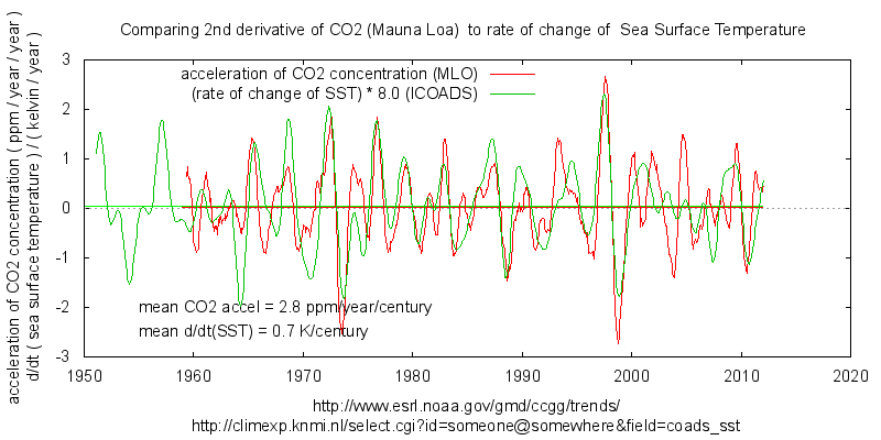
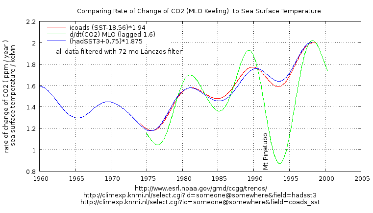
The water outgassing argument is more complex but you should at least be looking at SST not satellite derived TLT, MLT etc. several people have explored the similarity of d/dt(CO2) and temperature “anomaly”.
https://climategrog.wordpress.com/d2dt2_co2_ddt_sst-2/
The magnitude of the short term ratio is much stronger than the decadal scale ratio.
That much Salby get right. Where I remain unconvinced is on the centennial scale where I get the impression he is twisting the meagre facts to fit his hypothesis. That does not mean he is necessarily incorrect but his arguments are certainly unconvincing.
OH dear , too many links ??

Sure photosynthesising lifeforms are gagging for CO2 , the more they can get, the more their biomass will increase to exploit it. A negative f/b on increasing atm CO2. A lot of that is ocean based life as well.
The water outgassing argument is more complex but you should at least be looking at SST not satellite derived TLT, MLT etc. several people have explored the similarity of d/dt(CO2) and temperature “anomaly”.
“Where I remain unconvinced is on the centennial scale where I get the impression he is twisting the meagre facts to fit his hypothesis.”
It’s a moot point. The lion’s share of the observed rise has been since 1958, when accurate and direct means of measuring CO2 were established. In that time, the rate of change of CO2 to temperature relationship has held with extraordinarily high fidelity.
It may indeed be a fool’s game to try to match up with the pre-1958 record from the ice cores. There are no means of corroborating the ice core measurements – indeed, they do not agree with the other proxies, which have consequently been disparaged. I do not consider them validated. But, as pointed out above, there is no need for them anyway.
Somewhat of an over-statement.
Well there is a fairly good ‘high frequency’ correlation using global SST averages after filtering out the annual cycles. That would seem to justify more detailed, regional analyses of d/dt(CO2) vs dT. I have not seen any.
Also not that the wiggles which match are on top of a notable d/dt(CO2) currently around 2ppmv/year. That could be centennial scale adjustment or simply the anthropogenic input. More likely a mix of the two.
http://www.ferdinand-engelbeen.be/klimaat/klim_img/co2_T_dT_em_1900_2011_B.jpg
“…a fool’s game…”
Ferdinand was the fool, Bart, and he did it just for you! And as you can see, the hadcrut4sh data that he used gave a perfect match at the turn of the century. (a period of slow and stable carbon growth where smoothing would be negligible) Had he extended the graph back to 1850 the data would have matched back to then as well. Even the early twentieth century is not that far off and is consistent with what we would expect with much smoothing. According to the temp data, the carbon growthrate quadruples during this time period. This should give inflated numbers in the core (and it does)…
Bart, this has been a most painful comment page to read. It’s as though we have a bunch of grown men sitting down to play a game of chess and they don’t even know how the pieces move. For God’s sake, can they at least try to understand the argument they’re critiquing? (short hint istvan et al, the temps paused and so did the carbon growth rate) It would be really nice, Bart, if folks would take the time to listen to you, so that they can at least understand what the argument is. That might then make for an intelligent discussion…
(BTW, where’s ol’ you know who?)
Greg May 13, 2017 at 5:01 pm
“Somewhat of an over-statement.”
In the realm of stochastic analysis, this is as good as it gets. It is an extraordinarily high signal to noise ratio, given all the competing influences and bulk measurements.
afonzarelli @ May 13, 2017 at 5:17 pm
“It’s as though we have a bunch of grown men sitting down to play a game of chess and they don’t even know how the pieces move.”
Is it ever! I feel like Arthur Dent trying to teach scrabble to the cave men.
afonzarelli,
What you don’t mention is that the green line matches the observations a lot better than the red line. The green line is calculated from the emissions and the net sink rate as observed (assuming linearity in the early period too), the red line as from Bart’s formula.
If there are two competing possibilities for a reasonable match between theory and observations over a certain time span, it is normal to see if both also match over a different period. The emissions/sink rate and applying Henry’s law matches ice core and direct data over 800,000 years without any modification. Bart’s formula needs modifications (a different factor and offset) for every new period…
Ferdinand, all bets are off when it comes to early twentieth century carbon data. With the potential for smoothing during that time period who knows which of the three are the most accurate. One thing that can be said is the red line looks a lot more like the keeling curve than the other two…
Regarding deeper cores, what is your take on the impact of the biosphere on co2 levels going from glacials to interglacials?*
Who knows just what we’re dealing with on larger time scales. With a shorter time scale, like that since the LIA, the temperature relationship does just fine. We can calculate that the LIA was at least .7C cooler than the pause which is certainly a good ball park figure. We see that both carbon growth and sea level rise briefly go negative around the turn of the century. With ice cores the relationship holds wherever we have expectations of little smoothing. And to think all that i’ve just mentioned depends entirely on temperature trends of the last few decades—that should not be happening(!) And then there is the derivative plot itself. A near perfect fit with both variability and TREND features. (that’s a far cry from those who would curve fit the keeling curve to the giss data set) That’s a lot of coinkidinks that come together in one neat little package. And no amount of “hand waving” is going to make those coincidences go away…
*don’t forget to answer my question (☺)
“Bart’s formula needs modifications (a different factor and offset) for every new period…”
Perhaps. If, and it’s a big IF, the ice core data are reliable. But, that is not really a problem for me – regime changes do occur in massively nonlinear, chaotic systems.
It is a much bigger problem on Ferdinand’s side that the notion of tightly regulated CO2 levels for hundreds, if not thousands, of years is thoroughly inconsistent with the notion that they are supersensitive to our minuscule inputs over the past hundred or so years.
Bart:
regime changes do occur in massively nonlinear, chaotic systems
Except that in this case the system acts surprisingly linear to temperature changes over the past 800,000 years (~16 ppmv/K) and the system acts surprisingly linear to CO2 pressure changes in the past near 60 years (a tau of ~51 years)…
the notion of tightly regulated CO2 levels for hundreds, if not thousands, of years is thoroughly inconsistent with the notion that they are supersensitive to our minuscule inputs over the past hundred or so years.
The above linear response of ~51 years to any CO2 pressure change in the atmosphere deviating from the steady state is not fast enough to remove all human emissions in the same year as emitted, but has no problems to remove any one-time Pinatubo injection or even Tambora in a few years,
No problem either to follow the glacial – interglacial transitions at a “speed” of 0.02 ppmv/year (100 ppmv in 5000 years).
“Except that in this case the system acts surprisingly linear to temperature changes over the past 800,000 years …”
Begging the question.
“The above linear response of ~51 years to any CO2 pressure change in the atmosphere deviating from the steady state is not fast enough to remove all human emissions in the same year as emitted, but has no problems to remove any one-time Pinatubo injection or even Tambora in a few years,”
Massive self-contradiction.
Fonzie,
A very detailed study was done by Jochen Schmitt e.a. on two ice cores over the past 24,000 years, thus ecompassing the depth of the last glacial period and the deglaciation + most of the Holocene:
“Carbon isotope constraints on the deglacial CO2 rise from ice cores”
As preview:
http://epic.awi.de/30386/1/schmitt2012s_accepted_all.pdf
or with a (free) subscription direct from Science:
http://science.sciencemag.org/content/336/6082/711
Interesting
LGM-Holocene transition: +100 ppmv, δ13C change +0.4 per mil (growing biosphere).
Human transition: +110 ppmv, δ13C change -1.6 per mil (growing emissions)…
Bart:
Begging the question.
Vostok ice core (420,000 years) CO2 vs. T:
http://www.ferdinand-engelbeen.be/klimaat/klim_img/Vostok_trends.gif
Where most of the deviation from the trend is from the lags of CO2 after T changes, especially at the onset of a new glaciation…
(note that the 8 ppmv/K is for polar temperatures, global more around 16 ppmv/K)
Massive self-contradiction.
With a half life time of ~35 years for any CO2 injection in the atmosphere above steady state, the Pinatobo injection at ~ 0.05 Gt CO2 or 0.014 GtC or 0.007 ppmv was not even measurable. The largest eruptions in the past millions of years like the Tambora, even with a 100-fold emission over the Pinatubo, thus around 0.7 ppmv CO2, would desappear rapidly.
If we may assume a constant supply of ~0.1 GtC from all CO2 outgassing and all volcanic eruptions over the years, that is good for 2-3 ppmv increase over the steady state…
Response misplaced here. This thread is too long.
NL, dunno, Maybe there is lots of oil money to be made. Not by me. TY high praise never the less on this little post, on more shakey research footings than my last Fisker Nanotech post at CE ( where I am a true SME). Appreciate your comments on both. I do try to stay true to Beacon science roots. Helps with my now 13 issued US patents. Guess I have to update that again. Never understood why playing the person was equivalent to playing the issue. Graphic illustrations here this post.
NL
Have you parsed Hermann Harde’s recent paper that posits the alternate interpretation of IPCC data that results from Salby’s work? His conclusion is “Our analysis of the carbon cycle, which exclusively uses data for the CO2 concentrations and fluxes as published in AR5, shows that also a
completely different interpretation of these data is possible, this in complete conformity with all observations and natural causalities.”
Thanks Nic
I wish that more skeptics would get that the real fight and debate is on the ground you have selected to fight on.
There is a REASON why Parliment calls on you to testify… YOU DID SCIENCE!
unlike salby
Imagine if the collective brain power of WUWT focused on the real problem.
Instead these guys believe a YOU TUBE VIDEO.. WTF?
A video …That has not been written up
that has NO DATA
that has NO CODE
They like the answer Salby gives, so forget the details like SHOWING HIS WORK
Jeez
Do you realize that you do polemic, not dialog? Politics, not thoughtful discussion? Rhetoric, not science? Just checking. It’s funny how fatuous you are without having any sense of it. I learned long ago that one can’t teach others to see themselves.
How does a concentration stop?
ristvan have you considered that CO2 could be released by natural sources when environmental temperature is greater than a threshold level and absorbed by natural sinks when temperature is less than the threshold level. The behaviour above and below the threshold may be non-linear.
You appear to imply that Salby expects CO2 concentration “rate of change” to be related to temperature “rate of change” rather than the actual value of temprature on decadal time scales. The pause was at a warm level – a decadal pause in temp change could mean no change in the rate of CO2 release if CO2 release is related to temperature ?
makes sense….
I asked you to study Salby’s videos if you had not. Gave reference coordinates. Pathetic.
An interesting article. My critique includes:
1) “Dr. Murry Salby has been getting substantial attention in the climate blogosphere, for two reasons. First is his theory that at least 2/3 of the observed increase in atmospheric CO2 is natural and temperature induced.”
I disagree with Salby here. My view is that 100% of the increase is natural.
2) “The seasonality of the northern hemisphere terrestrial photosynthetic sink is apparent in the Keeling curve, as is the temperature/CO2 discrepancy disproving Salby.”
This is the old Al Gore theory. No, the seasonality is (obviously) due to Southern Ocean temperature changes.
3) “First, if Salby is right, the rise in atmospheric CO2 concentrations should have slowed or stopped because of the ‘pause’. They haven’t. They bear no short or long term relationship to one another.”
The temperature pause is a measure of land and sea surface temperatures. The sea surface temp has increased very slightly to give us the continuing rise as per the Keeling curve. Land surface temperatures have decreased slightly to give us the overall pause result. The lowering land surface temperature is a worrying trend given the recent lack of sun spot activity.
4) Nice to see some traditional science appears in this argument:
“Barren ocean regions are mainly influenced Henry’s Law and Le Chatellier’s Principle.”
Why the comment is confined to “barren oceans” is beyond me. HL applies to all water/atmosphere surfaces and LC is an integral part of the three dissolving stages of CO2 into the oceans.
If the seasonality was due to Southern Ocean temperature changes, then wouldn’t the seasonal variation in CO2 be highest over the Southern Ocean? It isn’t, it’s highest in the NH.
In fact the strongest annual swing is at Arctic sites like Barrow and Alert stations. So the same logic says that it is the cold water sink of the Arctic which is driving the global change, not the US or China burning coal.
And “global warming” is strongest in the Arctic. Doesn’t that mean that the Arctic is driving the warming not fictitious
“polar”Arctic amplification?https://climategrog.wordpress.com/co2_alert_fit/
Hi Mike,
The katabatic winds over the antartic during winter ensure the atmosphere is well and truely mixed.
Robert Beatty
That’s a pretty strong statement given that the Antarctic is a continent, whose total ice area (land + shelf +sea ice) alone at maximum sea ice is larger than all other land masses south of the equator.
Would Santa Ana winds in California affect the distribution of acid rain particles in Ontario? Only limited valleys around Antarctica have the high sustained winds that are advertised so frequently. Do the high waves photo graphed at some beaches off Australia mean every beach off of Australia has great surfing? If adiabatic winds occur at the base of individual glaciers in specific valley outlets… what is their speed and area 1000 kilometers away at the edge of the sea ice, and 5000 kilometers away , then 10000 kilometers away?
I’m serious:

Much of the weather of Europe and N. Am is driven by Arctic polar vortex. The typical land+ocean “global average” is biased in favour of land SAT because it is more volatile. That land bias means that he “global average” is NH biased. It is quite credible that Arctic polar vortex influences the defective “global average temperature” which everyone is bed-wetting over.
The 1998 super El Nino was pre-saged by a notable swing in N. Atl Oscillation:
Yes, but Mike, there is less ocean for co2 to sink into in the NH…
Greg – The statement referred specifically to Southern Ocean temperature change, not to anything else in the SH, so my comment was aimed at that. The seasonal swings in the far south, eg. Baring Head, S Pole, are not just lower, they are almost non-existent, while from the tropics to the far north they are high. I think that pretty well rules out the S Ocean as the driver. Yes, the strongest annual swing is in the far north. But that doesn’t necessarily mean that it’s the Arctic water that is driving, it could be the NH flora. The seasonal swings are not hugely different from Barrow to the equator, just a bit higher at Barrow. And I think you will find that Barrow is as close latitudinally to the NH flora as any other CO2-measuring station.
“I think that pretty well rules out the S Ocean as the driver.”
The tributaries of a great river are all small. The pileup of water occurs where resistance to the flow is greatest.
Life turns CO2 into coal, oil and the cliffs of Dover. That is a sink.
If warmer water is outgassing this will lead to a reduced sink and an increased dynamic equilibrium level. Just saying “sink” does not form a conclusive point.
Greg,
Implicit in your definition of a “sink” is the length of time the CO2 is sequestered. However, I have never seen anyone specifically define how long something needs to be sequestered to be considered a sink.
If you pore water down the sink and it comes back up in the toilet, the sink is still sink. You have a new source to take into account.
“First, if Salby is right, the rise in atmospheric CO2 concentrations should have slowed or stopped because of the ‘pause’. They haven’t.”
Now this makes me pause. If we know that natural causes do not stop and start rapidly (IE: 800 year lag), then any assumption that a rise in CO2, when the warming has stopped or paused, is man made would be totally in error. The degradation of plant matter would continue to force rise for many years even though the plants themselves would slow in growth. Salby’s model does not say there would be a slowing of CO2 rise. I am not sure where you came to this conclusion.
Again, too simplistic. Water is rising from the cold depths, sinking in the Arctic and absorbing or out-gassing at moderate latitudes. Area of exposed water in Artic has changes notably in recent decades.
If the discussion is Henry’s law ; Feck;s law etc. starting with UAH TLT is not the most relevant dataset.
Salby’s point there is that temperature affects the rate of change, the ppmv increase year to year. If the temperature plateaus, the yearly increase should remain about the same, not drop to zero as Rud suggests. I’ve plotted the annual data for all 12 months of the year, January to January to January, etc., and the correlation remains strong.
ristvan – Thanks. Good analysis, good article. To my mind too, Murry Salby’s numbers don’t stack up. I did a whole heap of calculations some years ago, and concluded that the late 20thC CO2 increase was something like 94% from man-made CO2, 6% from natural. One counter argument at the time was that the oceans were absorbing half the man-made CO2, so the natural contribution must be zero. This counter argument was incorrect, the point being that without the man-made CO2 the warming oceans would have provided an increase of around 6% of the actual observed. But this brings me to my main point in this comment. You say “The ice core based CO2 lagged change to temperature is about 800 years, common sensically corresponding to the thermohaline circulation period.“, and that seems to be generally accepted (but see [1] below), but I think there are two separate timescales. There is another much faster CO2 response to temperature from the upper layer of the ocean, as per Henry’s Law, Revelle Factor, etc. I worked out that it had a half-life of around 12 years – ie, that the ocean-atmosphere CO2 transfer was at a rate that would halve the ocean-atmosphere CO2 imbalance in around 12 years. Then there is a quite separate and longer timescale driven by the deeper ocean.
[1] Yes, this is the theory re the 800 years. I have never seen anyone explain the way it actually worked, ie. the mechanism. I must be missing something, because the CO2 transported by the THC and re-released after 800 years seems to have had to come from the ocean in the first place. So it could easily explain an 800-year cycle, but to my mind cannot explain an 800-year lag in a longer cycle.
It’s a hand-waving attempt to explain away the 800 lag and thus retain the idea that CO2 is driving temperature. Since we have not been doing deep ocean circulation observations for that long. I doubt even the 800y figure is anything more than a convenient guestimate. But hey, this is climatology, not physics.
I doubt that Hansen predicted anything that he did not rig in advance.
the lag wwas predicted by hansen
and its no problem.
watch this
Cool, statisticians realise that regressing two sets of error laden variables gives a biased estimation. When will climatologists account for that when regressing Rad on Temp and getting an exaggerated ECS?
Steven – At the time that Hansen predicted the 800-year lag, had it already been observed in the ice cores? It seems to me that prediction of something known is a bit easier than prediction of something as yet unknown.
I didn’t know that [if?] Hansen predicted the 800-yr lag. Can you find me a reference to that. If he did predict, that is very strong evidence that he knows what he is talking about.
“I didn’t know that [if?] Hansen predicted the 800-yr lag. Can you find me a reference to that.”
I think the allusion is probably to this Nature paper (Lorius et al) on which he was a co-author. It was in no doubt that the CO2 response was a feedback; they calculated that it contributed from 40-65% of the change. Their analysis didn’t depend on the phase relation, and I didn’t see one predicted. They say:
But I really don’t see the reason for making an issue of the phase lag. It has long been understood that ice age changes were caused by orbital changes, that CO2 changed in response to temperature mainly in the oceans. Here is the AR3, 2001, setting it all out:
“Orbital variations (Berger, 1978) are the pacemaker of climate change on multi-millenial time-scales (Hays et al., 1976). Atmospheric CO2 is one of many Earth system variables that show the characteristic Milankovitch periodicities, and has been implicated as a key factor in locking natural climate changes to the 100 kyr eccentricity cycle (Shackleton, 2000). Whatever the mechanisms involved, lags of up to 2,000 to 4,000 years in the drawdown of CO2 at the start of glacial periods suggests that the low CO2 concentrations during glacial periods amplify the climate change but do not initiate glaciations (Lorius and Oeschger, 1994; Fischer et al., 1999). Once established, the low CO2 concentration is likely to have enhanced global cooling (Hewitt and Mitchell, 1997). “
Terrific! A lecture on complex physical relationships by an economist! How quintessentially Mosher.
“Good analysis, good article.”
Mike, how can you of all people say that? i know that you know that it’s the RATE of carbon growth that varies with temperature. i also happen to know that you know that the mass balance argument is bunk. Other than those two arguments, there is not a whole lot else presented in Rud’s piece (save the satellite co2 data)…
(oh, yeah and that 800 year lag thing that just so happens to be missing in shallow ice cores)…
afonzarelli – Rud’s article was chiefly a crit of Murry Salby’s arguments, and I thought his analysis of those was good. I’m not sure which part of my temperature-CO2 knowledge you are tapping into re the “RATE of carbon growth that varies with temperature“. There is indeed a very strong correlation between annual change in atmospheric CO2 and temperature [as first(?) identified by Frank Lansner], which tallies exactly with what you say. But those annual changes in CO2 are really just wiggles on a trend where the trend is much larger in scale and tallies quite well with man-made emissions. So while I do think that some CO2 variation is T-caused, the great majority does seem to be man-made.
OTOH, I – like you apparently – am somewhat dubious about the 800-year lag.
afonzarelli – Sorry, I should have addressed your other point too – the mass balance argument. The mass must balance, but any particular set of mass balance figures may or may not be junk. My view is that there are too many unknowns for any of the proposed mass balances to be reliable. But then, Rud Istvan’s arguments don’t rely on a particular mass balance.
Mike, i oft quote you on the mass balance argument because you are the only person who has ever stumped ferdinand on it! Like FE, Istvan is saying that since the oceans are a net sink, they can’t be a source at all (zero, nada, nilch). Your argument (to ferdi) says that if even a small part of the rise depends on the existence of a natural imbalance, then the rise is at least part natural…
Also, you once produced a graph showing the close relationship of temperature to rate of change of the carbon growth rate. (i used to use it, but it confused people because it had temps lagging co2; i think it used a thirteen month median which ended up doing that) If what you’re saying is true, then there is no reason that your trends of temps and rate of changes (of co2) should match as well as the variability. Think about it. Now, what i’m saying doesn’t mean the rise is necessarily natural. It only means that the rise, anthro or not, is temperature dependant both short term and long term. And as more than a few comments hear have noted, Istvan dropped the ball on that point. (the pause in temps corresponds with a pause in the carbon growth rate)…
Mike Jonas, Frank Lansner wasn’t the first to recognise the CO2 thermometer in 2008, Jarl Ahlbeck wrote a contribution on John Daly’s website already in 2001
https://www.john-daly.com/co2-conc/updated.htm
afonzarelli,
Your argument (to ferdi) says that if even a small part of the rise depends on the existence of a natural imbalance, then the rise is at least part natural…
Seems a rather strange reasoning: in some years (like during an El Niño) the biosphere as a whole is a net source of CO2, but as the oceans still are a larger sink, even with warmer oceans, the net sum of all natural sinks and sources stil is a (small) net sink. Thus the natural contribution to the CO2 increase in the atmosphere even in El Niño years still is zero…
The only part where I can admit (with reluctance…) a natural contribution is the influence of temperature at a maximum of 16 ppmv/K per Henry’s law, as that would happen even without human emissions…
The average lag of atmospheric CO2 behind surface T evident in the Vostok core data doesn’t imply that it, along with water temperature, was transported virtually unmodified by THC, reappearing ~800yrs later at the surface. This is the “global conveyor belt” meme that is uncritically accepted in “climate science,” but is dismissed by qualified oceanographers as sheer fantasy. It completely ignores the highly stable temperature stratification of all oceans and the inevitable mixing of water masses in transport.
While there seems to be little reason to doubt that the secular rise of Mauna Loa CO2 is indeed primarily man-made, it’s relationship to modern-day surface temperatures needs to be clearly understood. Cross-spectrum analysis of season-suppressing yearly averages shows that delta-CO2 invariably LAGS surface T, when coherent, and is otherwise unrelated. The lag, however, is orders of magnitude less than 800yrs! Nevertheless, it falsifies the notion of CO2-driven T variations.
Because of the ice cores, the 800yr lag of CO2 behind temperature rise seems to have become a logical box that many can’t escape from. It is perfectly possible for their to be such a lag on this scale, but it doesn’t rule out that a coca cola from the icebox in a warm room with the lid off will become flat in an hour or so. Doesn’t the post 2016 El Nino show a measurable increase in CO2 over the pre El Nino as per an illustrate post above:

First two weeks of June 2015
First two weeks of June 2016
Or have I got this wrong.
That looks like less CO2 after the 2015-16 El Nino rather than more.
The atmosphere is all about chemistry, physics, heat transfer and thermodynamics. You want an expert trained in those topics, certified in those topics, whose career is actually applying those topics check with a experienced chemical or mechanical engineer.
The world is still recovering from LIA and has seen 300y of general warming. Ice core record shows a lag of around 800 years. Why do you expect atm CO2 to stop dead in its tracks on a sub-decadal timescale?
Since nowhere in the article do you seem to be examining d/dt(CO2) against temp. anomaly which was Sably’s basic point about orthogonality, it seems that you have totally missed to point of the work you are aiming to criticise.
Maybe you should have taken the time to dive deep before diving deep into counter arguments.
@ Greg
May 13, 2017 at 4:44 pm: Thanks Greg, that was a point I noticed too. Still waiting to learn if Salby was ever included in the debate as one would reasonably expect. We have no reason to be enemies.
I agree with ristvan,


Salby’s model is based on mathematical errors and logical errors.
The airborne fraction of human emissions to that remaining in the air of 2.2 to 1.0 falsifies the proposal.
The ice age CO2 ppm to Temperature ratio of 19 ppm to 1.0C falsifies the proposal.
The change in CO2 back to 0AD versus GISP2 temperatures does not lead to one to really any conclusion other CO2 likes to be at 280 ppm in non-ice age conditions.
The change in CO2 per year going back to 0AD versus human emissions clearly indicates we are responsible for the recent increase.
But then the natural absorption/release rates were many times bigger than our emissions until recently.
Overall, it appears the math works when one assumes that the natural level of CO2 in non-ice age conditions is about 280 or 275 ppm. When the concentration in the atmosphere rises, the natural absorbers begin to work harder and harder but all they manage is 1.8% per year of the excess above the equilibrium rate of 280 ppm.
We do no have to cut our emissions to Zero to stop the rise in CO2. The natural absorption rate will eventually catch up if we start limiting the growth in emissions. In the last three years, there has been no growth in human emissions so it is very possible with just more efficient natural gas power production for example.
Sorry Bill, your second graph is Mann-Jones hockey stick grafting two incompatible datasets in the same colour with no indication of what data is used nor that graft you have done.
No cookie.
Your third graph contradicts Ristcan’s claim that CO2 did not slow down during ‘the pause’. It did. I seems to have stabilised at around 2ppmv/year rather than the steady acceleration of late 20th c.
Also as emission controls start to bite and human emissions ease off in the last few years, the “actual” CO2 change rocket’s off again. On the crude scale you show this seems to correspond to the 2011-2015 “super El Nino”.
The annual CO2 increase is affected by the ENSO. It rises much less in a La Niña and much more in an El Niño.
Let’s say in average ENSO year right now, CO2 would increase by 2.3 ppm.
In an El Niño, this would jump to 3.0 ppm but in a La Niña it would increase by just 1.6 ppm.
But let’s go back to the biggest Supe-El Nino on record, 1877-1878. This was truly a remarkable El Nino. But CO2 only rose by 0.1 ppm in that year.
It obviously depends on human emission rates or actually more accurately, how far away the number is from equilibrium of 275-280 ppm.
But let’s go back to the biggest Supe-El Nino on record, 1877-1878. This was truly a remarkable El Nino. But CO2 only rose by 0.1 ppm in that year.
Bill, think about your sinks…and biology .when something like CO2 is limiting….plants, algae, bacteria, on and one…..grab it fast and more of it
The biggest problem I see, trying to compare now with then…when we really don’t understand either
That is a very foolish statement to make, since accurate atm CO2 only started in 1958. You still have not even said what the data you are using in your graphs is ( the early stuff you grafted on to Scripps data like it was the same thing ).
What time resolution does you data have ? It is presumably ice core of some sort. There are enormous questions about about firn closing times , diffusion etc. One that that is certain is that you do not have annual resolution and it will NOT capture the annual swing of that year.
Maybe we should look at an event for which we do have data. The 1998 event shows a massive swing in dCO2
https://climategrog.wordpress.com/co2_sst_regression_nino98/
Interesting stuff Bill, but how do we know CO2 numbers are that accurate?
7 years ago right here on WUWT, David Middleton made a guest post about CO2 levels of the past, showing that Ice core CO2 data are not that reliable,it is probably too low.
It is worth reading.
CO2: Ice Cores vs. Plant Stomata
https://wattsupwiththat.com/2010/12/26/co2-ice-cores-vs-plant-stomata/
I think the ice cores are accurate (can I say to the extent that the climate scientists haven’t mucked around with them like they have the surface temperature record).
Stomata appear to be reasonably accurate as well but then this depends on what time of the year the fossil specimens were laid down. On a local basis, CO2 can be as low as 250 ppm or as high as 2000 ppm. Throughout the day, one could see those kind of changes and throughout the seasonal cycle, one could see those type of changes.
The local vegetation will have responded to those levels but maybe they were buried at 9:00 am in early Spring and as a consequence they will indicate a high CO2 level.
Climate Science likes to use a proxy of Carbonate from fossil soils or paleosols. But this as well depends completely on the time of year and the precipitation levels that existed at the time the fossil soils were isolated and buried. The methodology can even record a completely impossible 0.0 ppm CO2 but climate scientists keep using it because they get to distort the record by using it. Really, they use a time series that contains 0.0 ppm 7 different times but 1,000 ppm on the other timelines but because they can cherry-pick, they keep using these fake paleosols numbers.
Stomata are100 times better than this and seem to match up reasonably well with what we know. But it is just not as accurate as the ice cores for an individual year like 1825 or 1080 or an average 1860 to 1880.
I think of stomata as being as secondary confirmer only.
Stomata from the Eemian show 330 ppm, if IIRC.
Thank you for your quick reply,Mr. Ellis.
The problem I see is the lack of Stomatal data,which is a shame since this is a significant Botanical response,to what is available at the time of ingesting the raw materials it needs for the Photosynthesis process. Surely they vary over time due to the regional environment they grew in, also varies. The Ice core data is TOO smooth ,when ALL other data from plants,chemical analysis ,shows significant variability as shown by David in his guest post.
David made the point in his guest post,that we lack precision and data to be sure the CO2 levels are actually a true marker of the atmosphere,at a point in time. That is why I think this needs to be investigated much more bringing in new data from various places,to develop a firmer data base with better resolution.
Rud, Dr Salby is correct. There is a natural source of CO2 which
increases with temperature.
First, a description of a recent experiment I performed on some decent
topsoil.
With a reasonably accurate CO2 meter, I measured the ambient CO2
at 6′, 406 PPM.
I then took a stainless steel salad bowl, inverted it and put the
CO2 meter under it, and put a 10 lb weight on the bowl.
12 hours later, I retrieved the meter. It read 1384 PPM.
Frozen ground stops the upwelling natural gas and greatly diminishes
or stops the microbial consumption of the gas which slows or stops
the production of CO2. Warm earth speeds the flow of natural gas
and encourages the microbes to bloom. The CO2 thus increases.
The atmospheric level of methane has greatly reduced its level of
rise. I believe increased microbial consumption that is more comfortable
in the warm topsoil is responsible.
Topsoil is not a sink for CO2, it is a source. My very simple and easily
replicated test proves this.
https://www.bing.com/images/search?view=detailV2&ccid=cE7lDPFa&id=
AD5AFF374A7573A0AF51BCCAA6DB23DE13F4E50F&thid=OIP.cE7lDPFa
YXj9Iqs2o46PBQEsCL&q=CH4+increase+vs+CO2+increase&simid=
608038495807210159&selectedindex=21&ajaxhist=0&first=1
I also agree with Dr. Salby on the reliability of ice core CO2 readings.
CO2 readings at ground level are highly localized, as my simple experiment
and historical leaf stomata prove.
Dr. Zibgniew Jaworowski’s work and my findings convinced me that the ice
core readings are useless.
http://www.warwickhughes.com/icecore/
With no sensitive historical readings of CO2, we do not know if the
current readings are even high. I doubt it.
Geological CO2 records are probably accurate but a blunt instrument.
Jerry, nice try but fail. Topsoil is at most 49 percent of CO2 sinks/aources. So your basic math fails on basic sink/source math.
Mr. Ristvan,
Your critique shows a lack of understanding of the processes involved. Salby said there is a lag at all time scales. This is not unknown. The CO2 is a dynamic quantity that changes rapidly locally and regionally driven by Primary Production, Respiration along with abiotic chemical and physical processes. OCO2 if you read the instruments description, only measures an average at the same places and times over a 16 day cycle to determine world co2. While this is interesting it doesn’t show the massive sources and sinks that exist but are regularly measured and evaluated by a wide number of people who are interested in trying to understand this very complex subject. I only post because you are not listening to someone who has a valid critique. Well done Mr. Hanson.
v/r,
David Riser
Jerry,
Please let Dr. Jaworowski rest in peace, together with his ideas about ice core CO2. He was an expert on radionucleides in ice, but as far as I know never performed any CO2 analysis. His remarks are mainly from 1992, completely refuted by the work of Etheridge e.a. on three Law Dome ice cores. Ice cores CO2 is reliable if you take a lot of precautions. There is even an overlap of ~20 years (1960-1980) with direct measurements at the South Pole…
Dr. Jaworowski made several real stupid errors like migration of CO2 from low to high levels, his “reason” why one measures too low CO2 levels in ice cores. If you measure 180 ppmv in the ice core bubbles and the outside atmopshere in the lab (or during storage) is 350-380 ppmv, how can CO2 migrate from inside to outside the ice core? See:
http://www.ferdinand-engelbeen.be/klimaat/jaworowski.html
Topsoil indeed is a source of CO2, but not more that in the previous year(s) leaves and other material was put down, thus that can’t release more CO2 than was captured first out of the same atmosphere. In general a null-operation and currently a net, growing sink for the whole biosphere.
CO2 readings at ground level are highly localized
Yes, therefore many of the historical measurements are worthless, as they were taken midst of towns, forests,… Only those taken on board of seaships and coastal with wind from the seaside are of interest. These show values around the ice core averages…
Modern measurements are made on top of barren mountains, ice deserts (Antarctica), islands in the middle of the oceans, in the atmosphere by airplanes, seaships,… They show little variation in the bulk (95%) of the atmosphere and mainly seasonal in the NH.
Ferdinand @ 10;50 am
The reason that CO2 levels are highly localized is that they are the result
of the hydrocarbons which perk up from deep in the earth being oxidized by
microbes.
This is not a theory of mine. I have proved it by experiment in different types
of topsoil. It requires work to dig through the topsoil, through any biomass
and worm castings.
The topsoil in Kansas I tested was more than a meter thick. Lots of digging.
Hydrocarbons perk up all around the earth, but they are not evenly distributed.
The shield in the area around Atlanta, Ga is close to the surface and blocks
the hydrocarbons. Very poor topsoil.
This is a very important finding, because it means that just about everything
you have read about topsoil is wrong.
A good example would be that the deep topsoil in Kansas was created
by deep rooted tall grass. The reverse is true. Over time and through
many fires and droughts, the plants with the deepest roots survived
when others did not, becoming dominate.
Because I do not have a PHD, I have not been able to garner interest
in my results. WUWT gives me a forum which I very much appreciate.
My findings mean that Dr. Thomas Gold was correct. Hydrocarbons do perk
up from deep in the earth and always have. The millions of years of layers
of carbonate rock witness that fact.
This means that hydrocarbons are a renewable resource and that we
will never run out. The Russians know and understand this fact and the
Saudis benefit from being on a fault which directs the heavier molecules
right to their fields.
What I request is that people who think that I am wrong find some good
upland topsoil and do a test.
It requires some work, but my findings are easily replicated.
“There is even an overlap of ~20 years (1960-1980) with direct measurements at the South Pole…”
Wow, a whole 20 years !!!! You have no idea about the long term (probably exponentially reducing but who knows) disolution of CO2 in ice under increasing pressures or assumed short term recovery rates in a lab. Nor has anyone else. Too many assumptions, limited credibility. Sorry, small round filing device in the corner,
“Ice cores CO2 is reliable if you take a lot of precautions.”. Circular logic. First understand and prove the physical processes at work in appropriate timeframes.
AJB,
Please, have some more digging in the scientific literature before commenting…
Ice core specialists are not stupid, they know the pitfalls and try as much as possible to avoid them.
Ice cores are laid down at -20°C for relaxation for at least a year. During that time, they expand with some 50% in volume. Most clathrates formed under the high pressure of ice then decompose again and bubbles regrow.
Ice core measurements are done by grating the still frozen ice under vacuum, freezing water vapor out over a cold trap and measuring CO2. That recovers about 70% of all gas and vacuum destroys near all remaining clathrates in the opened bubbles.
The alternative method is sublimating all ice under vacuum just under melting point with an IR lamp and cryogenically freezing everything out and later selectively evaporating each part and measuring everything on a mass spectrometer, thus including the isotope ratios. No CO2 can hide anywhere in that way.
I know 20 years is short, but already a good check for the best resolution (~10 years) ice cores of Law Dome, spanning the past 150 years. The next ice cores span ~1000 years (resolution ~20 years) and match the first over the most recent 150 years, The next core spans 70,000 years (resolution ~40 years) and match the second over the most recent 1000 years and then we have one of 420,000 years (Vostok) and one of 800,000 years (Dome C, resolution ~560 years). All these ice cores, with extreme differences in temperature, accumulation rate, layer thickness,… show the same CO2 levels for the same average gas age within a few ppmv, including a trapped check of each other.
Thus in my opinion, ice core CO2 levels are very reliable, but are (assymetric) averages of CO2 levels in the ancient atmosphere over periods between 10 and 560 years,
“No CO2 can hide anywhere in that way.”
Except that which likely already escaped by diffusive means (solute or gaseous) over extended time. I agree, we are looking at long term averages with limited resolution as indicated by stomata studies. Not sure what you mean by ‘assymetric’. But even if you improve the resolution, physical diffusive mechanisms will still have fudged out the variability over unknown, inconstant timescales. And since they’re not fully understood, possibly affected the longer term calibration too. Usual arguments reasonably well summarised here.
AJB,
Diffusion over time goes from higher to lower levels. If we measure 180-300 ppmv in ice cores, it is impossible that real levels in the atmosphere were below 180 ppmv, or C3 plants were in serious trouble. Worst case, the levels were higher, as in some periods the stomata data show. Migration from low to high levels? Dr. Jaworowski made that error, unbelievable for an ice core specialist.
The main advantage of stomata data is the higher resolution, the main disadvantage is that these are a proxy for local data on land, where there is in average a positive bias over “background” CO2, That is compensated for by calibrating the stomata data against ice core data and direct measurements over the past century. The problem is that nobody knows how the local bias changed with land (use) changes over the centuries in the main wind direction. Even the main wind direction may have changed in certain periods (MWP-LIA)…
Thus in my opinion, stomata data are good indications of more (local) variability and resolution than ice cores, but of the average of the stomata data differs from the average ice core data over the period of resolution of the ice core, the stomata data need recalibration, not the ice core data…
Assymetric: take the high resolution (~10 years) of Law Dome: the pores in the ice are gradually decreasing with depth and after 40 years so far closed that any migration virtually stops.
The first years, the enclosed air freely exchanges with the atmosphere, thus its age is the same as in the atmosphere. As the firn get denser, it takes more time to migrate, so the average age of the enclosed air lags the atmosphere and at 72 m depth (40 years ice layers), the migration stops at average 7 years older air than in the atmosphere with an average range of ~10 years for the bulk, with a long, small tail up to 40 years old air.
Bill Illis, this is a compelling and easy to understand presentation. Are you aware of the call for comments by the EPA on the Executive Order:
https://wattsupwiththat.com/2017/05/12/three-days-left-to-submit-suggestions-to-repeal-epa-regulations/
This is a perfect contribution, especially the issue of Natural Gas effect on CO2 accumulation in the atmosphere. I urge you to submit it. There is a link.
Ah… Satellites.
ristvan,
You said, “He observationally bolsters his conclusion by ‘showing’ that highest CO2 concentrations are over relatively uninhabited/unindustrialized regions like the Amazon basin, so must have natural origins. The following ‘observational’ figure is from his Hamburg lecture. Except it is completely disproved by OCO-2.”
I don’t see that your claim is supported by the released OCO-2 maps. If you go to http://wattsupwiththat.com/2015/09/15/are-the-oceans-becoming-more-acidic/ , and scroll down to the NASA/JPL illustration I provided, I think that you will find a resemblance to the Salby map. In particular, the Amazon Basin and southern Africa both show high levels of CO2, similar to Salby’s map.
CS, i provided links to NASA at the time. Even provided contemporary figures in the post. And then noted OCO-2 was even worse. What part of that do you not yet get?
OCO-2 does in fact show some of the highest CO2 concentrations over uninhabited WINTER forest regions. Lower Northern Hemisphere concentrations as in the depicted image are demonstrated in the summer, when photosynthesis is more active there.
Do note as well that generally increasing temperatures will promote significantly increasing microbial activity, which composes most of Earth’s biosphere and thus carbon cycle.
ristvan,
You asked, “What part of that do you not yet get?” Apparently none of it and I’m not a dimwit. So, ask yourself why the disconnect? You claimed that Salby’s Hamburg figure is “completely disproved by OCO-2.” I provided a link that, to me, bears a strong resemblance to Salby’s figure. If by “links” that you provided you mean the two figures, I can’t read the associated text even after zooming in 150%. Even so, what appears to be the most recent data, albeit with a different color scheme, is not all that different from the illustration in the link I suggested. So instead of reverting to your all too common arrogant response, please be more specific in how your “links” completely disprove Salby’s figure.
Yes, but Clyde, the amazon and congo are not sources of co2. They just pull it in out of the atmosphere and release it via dead biomass. (analogous to a back yard pond that collects debris but does not produce it)…
afonzarelli,
Sources and sinks can be interchanged with the seasons. You didn’t define “source.” Therefore, I’ll give you my definition: A CO2 source is any area on the surface that for at least part of the year has a CO2 concentration that is above the median, irrespective of the mechanism that is producing the CO2. Therefore, the Amazon Basin may be a sink and a source, but is acting as a source for the OCO-2 map I cited. Your pond example might be considered a ‘sink’ for debris. In a similar manner, the polar sinks do not produce the CO2 they are removing.
Clyde, the only reason that the amazon and congo are “acting” as sources in your map is that they gather co2 at those places and releasing it through dead biomass. In your map, those areas are not adding anything to the atmosphere that they haven’t taken from it first (save deforestation). That’s THE reason that they are showing up as dark red…
Clyde, let me add that what i’m saying is an aside to what you and istvan are specifically talking about. i’m just looking at the bigger picture. Not intending to be a distraction, i’m just trying to add some clarity for others who may be reading (or perhaps even yourself). At the very least it may be, as you are pointing out, that istvan has misrepresented salby on the particular issue that you have raised…
afonzarelli,
And by the same line of reasoning, the CO2 released in tropical waters by outgassing is “gathered” at the poles and is transported to the tropics where upwelling occurs. The amount of CO2 in the water is increased by “dead biomass” drifting downward through the water column, oxidizing by bacterial decomposition and being dissolved in the cold water that is under high pressure. There is no ‘new’ CO2 on the planet. It is all old CO2 that gets moved around. The Carbon Cycle is all about characterizing the transient sequestration and subsequent release. What is happening in the Amazon Basin is fundamentally no different from what is happening in the oceans. However, what is at issue here is whether or not Salby’s statement that most CO2 is being released into the atmosphere in areas with relatively low population densities is true or not. It seems to me that there is evidence to support Salby’s claim.
Well… Clyde, the oceans have a mechanism for being a source, outgassing. Sure, trees can become a source, too, by dying off (and not being replaced by new growth). i’m just trying to make it clear that those red areas in your map are not bonafide sources. They are adding nothing to the content in the atmosphere. (just as some argue that the oceans ain’t adding much to the atmosphere either)…
Let me ask you a question if i may (now that i have your attention)… What (say you) would atmosphereic carbon levels look like during an interglacial if the biosphere was the same as that during glacials? (IOW, what impact does sequestration by trees have on carbon levels as the planet warms from glacials to interglacials?) Thanx…
afonzarelli,
First off, I have to acknowledge that I miss-spoke. The amount of carbon is fixed, not CO2. However, the carbon changes its oxidation state as it is sequestered and potentially released into the atmosphere as CO2.
You said, “…those red areas in your map are not bonafide sources. They are adding nothing to the content in the atmosphere.” First off, you aren’t using the definition that I provided and you haven’t offered an alternative. If dead trees or leaf litter are being converted from carbohydrates to an oxide at a greater rate than surrounding vegetation is converting the CO2 back to carbohydrates , then I would say that the region in which it is happening is, at the very least, a transient source of CO2. Consider a situation where one is alternately opening and closing a valve on a tank of CO2 in a hot house. Isn’t the tank a source of CO2 for the plants in the hot house? It doesn’t have to be turned on all the time to be a “source!”
To answer your question about interglacials: Clearly, vegetation has the ability to draw down CO2 and reduce the atmospheric concentration. That is basically why we have coal. However, the whole point of trying to characterize and quantify the Carbon Cycle is to discover how all the various elements interact over time. The leaves in trees and annuals are a seasonal reservoir. The trunks of trees act as a reservoir with a life span of decades to hundreds of years. However, ultimately, the sequestered CO2 will be released. In a typical situation, the release and absorption of moderate-term sequestration is nearly in balance. However, consider a situation where a disease or insect infestation kills most of the trees in a forest in a short period of time. Then, the release of CO2 will not be neutralized and there will be an excess of CO2 over the production of carbohydrates. It is possible to have short-term and long-term imbalances in the re-cycling of carbon. That is what the whole AGW argument is about.
Ristvan, Is the Argo data before or after adjustment?
Argo matches bouys matches satellites matches re analysis matches ships IF you adjust the ships
Which doesn’t answer the question asked. 😉
Yeah, Mosher did. He took a sophisticated sideswipe at Karlization (2015). You need to know more.
A casual look at the Keeling Curve at the time of the last 3 El Nino events looks to me like it supports Salby:
https://qph.ec.quoracdn.net/main-qimg-e73e23b02785cb2195f8f0c526df1a8d
I drew the time of the last 3 strong el Nino events offset slightly below the main curve. each time the Pacific got warmer, the CO2 accumulation accelerated.
Yes , far bigger swing in 1998. Short term d/dt CO2 does show a strong temperature dependant signal. Sadly Rud did not even understand Salby’s main point before trying to dismiss it.
This short term variability is on top of long term rise. The question is : does the long term d/dt CO2 also contain a temperature driven component ( almost certainly it does ) and how much. Salby in unconvincing but raises valid questions.
gregfreemyer,
Your link doesn’t seem to be working.
gregfreemyer,
The point is that the observed variability is not more than +/- 1.5 ppmv around a 80 ppmv trend for the extremes (Pinatubo, El Niño) and more important, levels off to zero in 1-3 years. The variability in CO2 rate of change has no influence at all on the huge CO2 trend, neither on the derivative, which still is around 50% in average.
If one calculates the net sink rate (in ratio to the CO2 pressure in the atmosphere above the equilibrium per Henry’s law) and subtract that from the yearly human emissions the residual plot is in the middle of the variability:
http://www.ferdinand-engelbeen.be/klimaat/klim_img/dco2_em6.jpg
Ferdinand,
I’m a bit confused. The chart for dCO2/dt(12) obs looks extremely reminiscent to the satellite temp chart. That seems to support the contention that a significant portion of dCO2/dt(12) is driven by temps.
gregfreemyer,
You may assume that most of the variability in CO2/dt(12) is driven by temperature variability. The point is that the variability is small, as your chart also shows: some 1.5 ppmv from the trend for the extreme El Niño’s but also 1.5 ppmv to the other side for the Pinatubo injection.
Over periods longer than 1-3 years the variability practically averages to zero around the trend of ~90 ppmv over the full period.
The error Salby (and Bart) makes is thinking that the match of the variability means that the trend also is caused by temperature. But human emissions in the same period are twice as high and the small increase in temperature never can push 90 ppmv extra in the atmosphere…
The trend matches, too. There is no justifiable reason to arbitrarily dismiss it, filter it out, and substitute your own preferred (and nonphysical) version of what you think the dynamics should be.
Bart,
Either compare T to CO2 or dT/dt to dCO2/dt.
Don’t compare T to dCO2/dt. You still have all the variability in T and CO2, which is the same in dT/dt and dCO2/dt. only shifted back in time. But the trends have nothing to do with each other: you compare the small trend in temperature with the small residual trend in dCO2/dt after removing the bulk of the trend of CO2.
All what you have done is declaring that the two (linear) trends match, so, the integral of T must represent the increase of CO2, which is based on a real correlation between the +/- 1.5 ppmv noise and the arbitrary match of two linear slopes.
That may work in an arithmetic world where you live. In the real world, variability and slope are caused by different processes: the variability mostly by the reaction of (tropical) vegetation on fast temperature changes, while the slopes are NOT caused by vegetation as that is a net sink over periods longer than 1-3 years…
“Either compare T to CO2 or dT/dt to dCO2/dt.”
Why? The data are what they are, and they match T to dCO2/dt.
You are forcing the data to fit your hypothesis, rather than your hypothesis to fit the data.
If you have been around in 1905, you would have told Einstein that everyone knows time progresses uniformly across the universe, and he had to shoehorn the data into that paradigm.
Nature is strange, and often fails to live up to our intuition.
Does anyone know from when we could accurately measures CO2 levels in the atmosphere ? It certainly wasn’t in the early 1900s. You cant tell me that in 1910 we had the technology to measure the % of CO2 to a one hundredth of a percent ? If we couldn’t accurately measure CO2 prior to 1940, then the values before that are invalidated. But let’s assume CO2 has increased by 100pm – then that is a change of 0.01% of a component of the atmosphere in a century. I think you will find both Oxygen and Nitrogen level have fluctuated by FAR bigger amounts over that time (and probably Argon too). While I don’t believe his theory, I also find it hard to believe that changing a component of the atmosphere by one hundredth of one percent has any impact what so ever.
Local measurements with some accuracy were made in the 19th century by the direct chemical method:
https://link.springer.com/chapter/10.1007/978-1-4757-1915-4_4
http://3.bp.blogspot.com/_Lxqre8hMG3M/Sz-Ovumj9QI/AAAAAAAABDA/l8bxjtZBsJw/w1200-h630-p-k-nu/weatherCO2historicalRawMeasurements.jpg
“First, if Salby is right, the rise in atmospheric CO2 concentrations should have slowed or stopped because of the ‘pause’. They haven’t.”
According to this study it did slow down and that while the human fraction of emission is decreasing.
https://www.nature.com/articles/ncomms13428
It’s not only according to this study. It is not controversial at all that the annual atmospheric CO2 change rate slowed down since ~1998. It’s basically flat just like the global temperature indices (no surprise since there is such a good correlation). This has happened during a significant increase in anthropogenic emissions, moreover an acceleration. So, the airborne fraction decreased. This is the opposite of what the consensus projected.
What happens next? Cooling and a decrease in the atmospheric CO2 change? Much smaller airborne fraction (zero, negative)?
This is also shown in one of Bill Illis’ graphs above.
Note how dCO2 takes off during recent El Nino when emissions are slowing or even constant.
It’s decreasing again with the temperature downturn. The annual growth and the AF will be low in 2017.
http://www.woodfortrees.org/plot/esrl-co2/mean:12/derivative
Rud is wrong on that point, but that doesn’t imply that Salby (or Bart) are right.
The net sink rate of CO2 in the atmosphere depends of the extra CO2 pressure in the atmosphere above (dynamic) equilibrium and the equilbrium depends of temperature. If human emissions remain constant, as was the case in the past years, still CO2 increases in the atmosphere and thus the net sink rate increases at a relative constant temperature. El Niño / La Niña and Pinatubo are only temporarely variabilities which zero out in 1-3 years.
See the graph in my previous message.
If human emissions remain constant for a long period, the airborne fraction indeed would go to zero until human emissions and sinks are equal.
If emissions would be zero tomorrow, there would be a drop of ~2.15 ppmv the first year, gradually decreasing until the CO2 levels are back in equilibrium with the current average ocean temperature.
“Rud is wrong on that point…”
Hear that, Istvan? Even Ferdinand is dumpin’ on ya! Admit that you’re wrong and move on (either that or keep your yap shut on GMOs, cause you can’t be trusted with that either)…
Rud Istvan, thank you for your essay.
sorry OP but biomass sinks increase emissions year on year in a warming climate. The trend of emitted CO2 is going up since the 1910 1940 warming and slight warming there after, it takes decades for nature to respond to warming with population growth relatively speaking per species ect.Take one insect that produces CO2 and calculate its growth from 1900 to 2017, I’ll reckon you’ll find significant and exponential contribution of CO2 by said species. Then do same for every net emitting lifeform. Lets see what numbers a model spews out
Rud Istvan:
I write to dispute two assertions in your above post; viz. you write
and
Before explaining why I refute those assertions, I point out that one of our 2005 papers made the same conclusions as Salby later asserted
(ref. Rorsch A, Courtney RS & Thoenes D, ‘The Interaction of Climate Change and the Carbon Dioxide Cycle’ E&E v16no2 (2005) )
That paper provides six models of the carbon cycle system. There are three basic models and they each assume a single mechanism dominates the cabon cycle system. In each basic model it is assumed that
1. the rise is purely natural
and
2. there is a significant anthropogenic contribution to the rise in atmospheric CO2 concentration.
Thus we provided six models.
Each of the models in that paper matches the available empirical data without use of any ‘fiddle-factor’ such as the ‘5-year smoothing’ the UN Intergovernmental Panel on Climate Change (IPCC) uses to get its model (i.e. the Bern Model) to agree with the empirical data.
The superior performance of each of our models over the IPCC’s Bern Model results from our modelling assumption. The Bern Model uses the assumption of anthropogenic CO2 emissions being in excess of what nature can sequester (which as I explain below is now refuted by the OCO-2 data). Our models assume something has altered the equilibrium state of the carbon cycle system.
Some processes of the carbon cycle system are very slow with rate constants of years and decades. Hence, the system takes decades to fully adjust to a new equilibrium. The observed rise in atmospheric CO2 is easily modeled as being continuing slow adjustment towards an altered equilibrium. And the decades of delay between an alteration to the equilibrium and achievement of the new equilibrium means that e.g. the ‘Pause’ would NOT have induced the rise in atmospheric CO2 concentrations to have slowed or stopped.
This raises the question as to what may have altered the equilibrium of the carbon cycle.
One possibility is the anthropogenic CO2 emission. In our models the short term sequestration processes can easily adapt to sequester the anthropogenic emission in a year because the dynamics of the seasonal variation strongly suggest this is true (and as explained below is now confirmed by the OCO-2 data). But, according to our models, the total emission of that year affects the equilibrium state of the entire system with resulting rise in atmospheric CO2 concentration as is observed. This possibility is real but unlikely.
Natural factors are more likely to have caused the alteration to the equilibrium of the carbon cycle system. Of these, the most likely cause is the centuries-long rise in global temperature which is recovery from the Little Ice Age. Almost all the CO2 flowing in the carbon cycle is in the deep oceans and adjustment of equilibrium between deep oceans and atmosphere would take several decades.
And the satellite data supports the understanding that the short term sequestration processes can easily adapt to sequester the anthropogenic CO2 emission in a year. It is not relevant whether, as you say, “satellites have NOT generally observed higher CO2 concentrations over uninhabited/ unindustrialized regions in past two decades”. It is important to note that the satellite data show some major industrialised regions (e.g. Western Europe) have LOWER atmospheric CO2 concentrations than some unindustrialised regions (e.g. Central Africa). This would not be observed if the emissions from human industries were overloading the sequestration near to their emission sites. The observation is consistent with emissions from industrial activity being completely sequestered in the regions where they are emitted (at least,they are in Western Europe) so they cannot be overloading the sequestration processes in those regions and,therefore, they are not available to overload the sequestration processes in other regions.
As mentioned above, each of the models in our paper matches the available empirical data without use of any ‘fiddle-factor’. But if one of the six models of our paper is adopted then there is a 5:1 probability that the choice is wrong. And other models are probably also possible. Also our six models each give a different indication of future atmospheric CO2 concentration for the same future anthropogenic emission of carbon dioxide.
Data that fits all the possible causes is not evidence for the true cause. Data that only fits the true cause would be evidence of the true cause. But the above findings demonstrate that there is no data that only fits either an anthropogenic or a natural cause of the recent rise in atmospheric CO2 concentration. Hence, the only factual statements that can be made on the true cause of the recent rise in atmospheric CO2 concentration are
(a) the recent rise in atmospheric CO2 concentration may have an anthropogenic cause, or a natural cause, or some combination of anthropogenic and natural causes,
but
(b) there is no evidence that the recent rise in atmospheric CO2 concentration has a mostly anthropogenic cause or a mostly natural cause.
Hence, using the available data it cannot be known what if any effect altering the anthropogenic emission of CO2 will have on the future atmospheric CO2 concentration. This finding agrees with the statement in Chapter 2 from Working Group 3 in the IPCC’s Third Assessment Report (2001) that says; “no systematic analysis has published on the relationship between mitigation and baseline scenarios”.
Richard
Thanks Richard, It’s amazing what you can learn if you don’t start out by thinking that you know what the answer is and inducing it into your method.
Shame the paper is paywalled .
If you have a pre-print, please drop me contact on my about page
https://climategrog.wordpress.com
Greg Goodman:
Thanks for that.
I cannot send you a copy of the actual paper because I am now on the Editorial Board of E&E and the publisher would take a dim view of my giving away copies.
However, my presentation to the first Heartland climate conference (2009) was an explanation of that paper and was accompanied by a ;paper which is almost entirely copy&paste from it. You can see me giving the presentation here and I will try to provide a copy of its accompanying paper at the link you provide.
Richard
Greg Goodman:
I cannot find an email address at your link. Please email me at RichardSCourtneyATaol.com but replace AT with @. I will attach the presentation paper to my reply.
Richard
Richard, I just saw your presentation. I was impressed and quite convinced. (it had only less than 100 views, how odd!)
Thanks
101,,,, 🙂
Richard,
I just took a look at your video. I think that you missed your calling. You should be a ‘man of the cloth!’ 🙂
Clyde
Clyde Spencer:
I am.
Richard
Clyde Spencer:
In retrospect I think my reply to you could be misunderstood as being facetious and, therefore, I write to clarify.
I earned my income throughout my adult life as a practicing scientist. Most of my research was conducted at the UK’s Coal research Establishment. Following closure of the UK’s coal industry I acted as an consultant on effects of energy production and coal use providing advice mostly to governments and politicians.
The reason I could provide the parody of a ‘fire and brimstone’ sermon is because I am an Accredited Methodist Preacher: I am currently Listed on the Plan of the Falmouth and Gwennap Circuit. During the closure of the UK coal industry the Methodist Church appointed me as an Industrial Chaplain.
Please note that I have never – and would never – provide a real sermon of the ‘fire and brimstone’ type.
Richard
Richard
The Autumn and Winter CO2 emissions do not accumulate over Eurasia. No-one has ever seen the peak value if they were to accumulate. The CO2 is transported away constantly by the passing winds and ultimately finds its way to the Arctic or Equator. Look at some of the CO2 charts from the link below. Those sample sites from the mid, and particularly the higher latitude.
You will note that the CO2 curve goes flat and between December and February. That is not accumulation, it is simply what is in the passing wind.
Rud’s conclusion that the land and ocean sinks cannot respond quickly, based on the +- 800 year lag coming out of a glacial cycle is completely irrelevant and misleading, and should not even be used as a comparison. Anyone that is familiar with equilibriums would know this as natural instinct. Those conditions are completely different, from the current state of equilibrium. Currently the interglacial is mature, oceans and land mass warmer and more surface interface area exposed, and ecosystems mature with reduced vegetation mass.
Coming out of an interglacial there is a lower volume of CO2 in the atmosphere as all biospheres are blooming and starving of CO2 is locked up in the sinks. The state of equilibrium could not be more different.
I work with various equiliriums on a near daily basis and they act identically, especially when the surface interchange area is reduced compared to the volume of fluid, there is a reduced concentration in the fluid for a period.
Within the equilibrium dynamics, there is active CO2. That is, CO2 that can move between the sink and tranport fluid readily.This is on a minute / hourly / daily basis.
It should also be remembered that the atmosphere is a not a sink, it is a transport mechanism between the sinks, and that CO2 has a relative saturation / density relationship between the atmosphere and the various sinks controlled by temperature. Given the surface interface area of the ocean and land the volume of active CO2 in the time required is completely feasible.
There is nothing in Ruds conclusion to convince me otherwise. .
Further, the images of CO2 that are used in the head post are not from OCO-2, as this satelite was launched in 2014.
There is still no discussion on the increasing volumes of CO2 at high ALTITUDES of 100km. The carbon cycle must be studied in full, not just the simplistic side.
https://www.esrl.noaa.gov/gmd/dv/iadv/graph.php?code=HPB&program=ccgg&type=ts
ozonebust:
You say
and
I strongly agree. The following are the basic mechanisms we considered in our paper I described above.
Mechanisms of the carbon cycle
The IPCC reports provide simplified descriptions of the carbon cycle. In our paper, Rörsch et al. (2005), we considered the most important processes in the carbon cycle to be:
Short-term processes
1. Consumption of CO2 by photosynthesis that takes place in green plants on land. CO2 from the air and water from the soil are coupled to form carbohydrates. Oxygen is liberated. This process takes place mostly in spring and summer. A rough distinction can be made:
1a. The formation of leaves that are short lived (less than a year).
1b. The formation of tree branches and trunks, that are long lived (decades).
2. Production of CO2 by the metabolism of animals, and by the decomposition of vegetable matter by micro-organisms including those in the intestines of animals, whereby oxygen is consumed and water and CO2 (and some carbon monoxide and methane that will eventually be oxidised to CO2) are liberated. Again distinctions can be made:
2a. The decomposition of leaves, that takes place in autumn and continues well into the next winter, spring and summer.
2b. The decomposition of branches, trunks, etc. that typically has a delay of some decades after their formation.
2c. The metabolism of animals that goes on throughout the year.
3. Consumption of CO2 by absorption in cold ocean waters. Part of this is consumed by marine vegetation through photosynthesis.
4. Production of CO2 by desorption from warm ocean waters. Part of this may be the result of decomposition of organic debris.
5. Circulation of ocean waters from warm to cold zones, and vice versa, thus promoting processes 3 and 4.
Longer-term process
6. Formation of peat from dead leaves and branches (eventually leading to lignite and coal).
7. Erosion of silicate rocks, whereby carbonates are formed and silica is liberated.
8. Precipitation of calcium carbonate in the ocean, that sinks to the bottom, together with formation of corals and shells.
Natural processes that add CO2 to the system:
9. Production of CO2 from volcanoes (by eruption and gas leakage).
10. Natural forest fires, coal seam fires and peat fires.
Anthropogenic processes that add CO2 to the system:
11. Production of CO2 by burning of vegetation (“biomass”).
12. Production of CO2 by burning of fossil fuels (and by lime kilns).
Several of these processes are rate dependant and several of them interact.
At higher air temperatures, the rates of processes 1, 2, 4 and 5 will increase and the rate of process 3 will decrease. Process 1 is strongly dependent on temperature, so its rate will vary strongly (maybe by a factor of 10) throughout the changing seasons.
The rates of processes 1, 3 and 4 are dependent on the CO2 concentration in the atmosphere. The rates of processes 1 and 3 will increase with higher CO2 concentration, but the rate of process 4 will decrease.
The rate of process 1 has a complicated dependence on the atmospheric CO2 concentration. At higher concentrations at first there will be an increase that will probably be less than linear (with an “order” <1). But after some time, when more vegetation (more biomass) has been formed, the capacity for photosynthesis will have increased, resulting in a progressive increase of the consumption rate.
Processes 1 to 5 are obviously coupled by mass balances. Our paper assessed the steady-state situation to be an oversimplification because there are two factors that will never be “steady”:
I. The removal of CO2 from the system, or its addition to the system.
II. External factors that are not constant and may influence the process rates, such as varying solar activity.
Modelling this system is a difficult because so little is known concerning the rate equations. However, some things can be stated from the empirical data.
At present the yearly increase of the anthropogenic emissions is approximately 0.1 GtC/year. The natural fluctuation of the excess consumption (i.e. consumption processes 1 and 3 minus production processes 2 and 4) is at least 6 ppmv (which corresponds to 12 GtC) in 4 months. This is more than 100 times the yearly increase of human production, which strongly suggests that the dynamics of the natural processes here listed 1-5 can cope easily with the human production of CO2. A serious disruption of the system may be expected when the rate of increase of the anthropogenic emissions becomes larger than the natural variations of CO2. But the above data indicates this is not possible.
The accumulation rate of CO2 in the atmosphere (1.5 ppmv/year which corresponds to 3 GtC/year) is equal to almost half the human emission (6.5 GtC/year). However, this does not mean that half the human emission accumulates in the atmosphere, as is often stated. There are several other and much larger CO2 flows in and out of the atmosphere. The total CO2 flow into the atmosphere is at least 156.5 GtC/year with 150 GtC/year of this being from natural origin and 6.5 GtC/year from human origin. So, on the average, 3/156.5 = 2% of all emissions accumulate.
The above qualitative considerations suggest the carbon cycle cannot be very sensitive to relatively small disturbances such as the present anthropogenic emissions of CO2. However, the system could be quite sensitive to temperature. So, our paper considered how the carbon cycle would be disturbed if – for some reason – the temperature of the atmosphere were to rise, as it almost certainly did between 1880 and 1940 (there was an estimated average rise of 0.5 °C in average surface temperature).
It is that temperature effect I mentioned in my above post.
But the effect of temperature on atmospheric CO2 emission would be very different in an Ice Age because all the processes 1 to 7 and processes 8 and 10 would be different. There is no data which indicates seasonal variation in the last Ice Age and, therefore, the relationship of temperature and CO2 cannot be determined for that climate state.
Richard
Richard,
A good qualitative summary of the Carbon Cycle. One small quibble, however. The volcanic CO2 is probably the result of melting of subducted sediments with entrained hydrocarbons and carbonates. Thus, it is a natural mechanism for releasing CO2 that has been sequestered for a very long time. Not unlike slightly acidic rain falling on the White Cliffs of Dover, and other terranes composed of limestone, and releasing CO2 when the chalk is dissolved, the rate of which all increases with increasing temperature.
I think that the role of underground coal fires is vastly underappreciated by the CAGW community.
I had made a remark above that no one seems to have picked up on. At least no one has taken me to task for it. That is, anthropogenic CO2 must have a moderating effect on outgassing from the oceans by increasing the partial-pressure of CO2 in the atmosphere. Therefore, to the extent that anthro-CO2 is suppressing outgassing, in the absence of anthro-CO2, one should expect that an equivalent amount of CO2 would be released anyway. Again, it would seem to be temperature that is the ‘control knob’ on temperature, not CO2.
Clyde Spencer:
You say to me
Yes, as I said in my first post in this thread
Simply, if that is the true cause then atmospheric CO2 concentration would be THE SAME if the anthropogenic emission were absent.
Richard
Odd the cult of CAGW ignores logic in peer reviewed paper that does not support their cult beliefs.
No need to worry. Mother nature will help settle this silly argument. The solar cycle has been interrupted.
Odd the IPCC assumed the CO2 absorption systems are saturated and does not scale in proportion to CO2 emissions to create CAGW where the ‘Bern’ equation was created to push CAGW, fake science.
The Bern equation for CO2 sinks and sources is fake science, ridiculous.
https://www.heartland.org/_template-assets/documents/publications/HardeHermann%20CarbonCycle%20ResidenceTime.pdf
Global and Planetary Change 152 (2017) 19–26
The annual (seasonal) cycle in atmospheric CO2 simply does not balance out. Why would it? There is an annual residual, depending on the global temperature average.
http://oi57.tinypic.com/28whxtx.jpg
Mr Salby (and followers)
I`m sorry that I have been so wrong about climate history. I couldn`t understand how much CO2 there was in the atmosphere during the holocene maximum and during the medieval maximum. Sure it must have been close to 450 ppm and 350 ppm. So I didn`t realize how wrong the proxy CO2 data were.
Or perhaps it was the temperature data I was so wrong about. Sorry that I didn`t understand how cold oceans were, when I thought they were warmer than today. So I didn`t realize how wrong proxy tempeature data were, and I didn`t realize how right the hockeystickers were.
So Mr Salby, can you forgive me my mistakes?
nobodysknowledge: “Sorry that I didn`t understand how cold oceans were, when I thought they were warmer than today.”
Perhaps you meant to use a /sarc there? These ocean waters were warmer according to this paper – http://science.sciencemag.org/content/342/6158/617
We show that water masses linked to North Pacific and Antarctic intermediate waters were warmer by 2.1 ± 0.4°C and 1.5 ± 0.4°C, respectively, during the middle Holocene Thermal Maximum than over the past century. Both water masses were ~0.9°C warmer during the Medieval Warm period than during the Little Ice Age and ~0.65° warmer than in recent decades.
Temperature drives CO2 up and down … a little.
It’s Dr. Salby.
No.
no,
no,
no,
no,
no,
no,
<a href="http://www.ferdinand-engelbeen.be/klimaat/correlation.html"no &
no etc.
I wish he were right, it would be most convenient, but sadly he isn’t.
http://www.ferdinand-engelbeen.be/klimaat/klim_img/Vostok_trends.gif
rats, I knew I would get the HTML tags wrong somewhere! ;o)
I have not had time lately to read as many articles here as I have in times past, and so have limited myself to the more interesting ones. (usually the more contentious ones) And this article was a gold mine of contention!
Having read every comment up to the point I write this, I am reminded of the singer-songwriter Paul Simon who observed: “man sees what he want to see and disregards the rest”.
I fear that “science” will lose its respect among the public as they finally see what a load of “wet, hot mess” climatology has become. Especially considering the utter BS we see from the English majors and the Divinity students in the argument. (looking at you Al Gore and others)
Scientists have long benefited from a respect and authority that few of them merit. One of the great gains of climategate is that we see who is behind the curtain.
Good points Greg.
Greg, Scientists of an earlier generation built up the respect you refer to. It has been degraded considerably in recent times.
Rud, Perhaps I was not specific enough. The only part of Dr. Salby’s
statements I agree with, based on my research, is that there is a source
of CO2 which increases with warmth.
The USEPA says that upland topsoil is a 30TG/yr methane sink. This
is based only on finding a flammable hydrocarbon in the topsoil.
This assumption fails a simple thought experiment. CH4 is much lighter
than air, when it hits the air, it rises.
My statement that the hydrocarbons in topsoil upwell from below
is based on experiment, not theories or models.
My challenge still stands. I will drive to your dairy farm and we can do
some actual experiments. with you operating the test meters.
You are soo sure of your opinions, test them!
The richness of topsoil, in the presence of adequate moisture,
depends upon the amount of hydrocarbons upwelling through
them.
I do not directly disagree. My simple point was that your moist topsoils are at best less than 40 percent of land ( the rest is tundra, drylands, and deserts (like Sahara, Rub al Kahli, and Atacama [I did not bother to look up the ratios] and land is only ~29% of earths surface. So please, just do some order of magnitude math. Then get get back on Salby’s global CO2 assertions. You cannot get there from here using any real data. Period. Proven in the guest post. How many times do you want it proven in more geanular detail?
The interesting thing about this whole discussion is that for Skeptics/Climate Realists, it doesn’t really matter what the actual cause of rising CO2 is (my guess is some combination of man and nature), because it doesn’t appear to be having much, if any effect on climate anyway. So for us, the argument is somewhat moot from a policy point of view, and becomes a purely scientific exploration, which is fascinating in itself. But the poor CAGW crowd are left out in the cold since for them, from a policy standpoint it very much does matter, which is why they have to attack it.
Bruce,
The attribution of source is important because there are many who want to ban the use of fossil fuels based on the assumptions that CO2 is having a significant impact on temperatures and that the CO2 increases are do almost entirely to humans. Being able to demonstrate that either hypothesis is wrong knocks the support out from under those clamoring for an energy revolution. That is important because bloodless revolutions are rare.
Like you, I believe that the rising CO2 is a “combination of man and nature.” However, I believe that the relative influence of anthropogenic CO2 is less than generally claimed because Anthro-CO2 is moderating the release of CO2 from outgassing and warming temperatures are increasing both outgassing and the release of biogenic CO2 from soils. We are currently in an adjustment transition seeking a new equilibrium.
Yes, Clyde, if we see an extended cooling spell and the carbon growth rate tanks right along with it, then it should be interesting to see where things go politically…
Atlantic Ocean CO2 uptake reduced by weakening of the meridional overturning circulation
http://www.nature.com/ngeo/journal/v6/n2/abs/ngeo1680.html
“If we knew what we were doing, we couldn’t call it ‘research’.” – Albert Einstein
Lordy. Not even a mention yet of the IPCC term “well mixed”, Rud?. Salby doesn’t even matter without addressing that question. Most of what happens below Mauna Loa actually stays below Mauna Loa.
Most of the arguments pretend this is not a problem. Yet if atmospheric CO2 was truly well mixed, then there would be no good justification for the existence of the OCO-II satellite. But if human CO2 emissions were located, say, at a point source in the far South-Atlantic Ocean during winter then they would probably vanish without trace. It s obvious that where and when the emissions take place does make a difference to any overall change in atmospheric CO2 concentrations. The arguments about what Salby may have got wrong mostly obscure this.
Does rain forest burning in Indonesia contribute the same amount of atmospheric CO2, per gram of locally-oxidized carbon, as Leonardo Decaprio’s goldfish? No, it doesn’t. But the EPA social cost of carbon is going to be used to attempt to tax you as if they were physically equivalent.
Salby is right.
After spending a fare amount of time reading the above, I think you are correct, or at least, he seems to be more right than wrong.
It seems that by choosing a season you can get whatever CO2 map you want.
Here is OCO for Oct – Nov, 2014
Just look at all those factories, cars, lorries and megacities in Amazonia, Congo, Indonesia and The Phillipines belching out all that anthropogenic CO2.
Just look at all those pristine unpopulated wildernesses in North America and Europe with low CO2, saving the planet. Especially the UK which seems to have the lowest CO2 on the planet – clearly no emissions happening there.
I think those factories are “plants” as in trees, etc.
Or those damn termites.
Tropical forests, aka jungles, are absorbing as much CO2 as we throw at them, and thanking us for the free food:
http://www.dailymail.co.uk/sciencetech/article-2891432/Carbon-dioxide-emissions-help-tropical-rainforests-grow-faster-Study-shows-trees-absorb-greenhouse-gas-expected.html
ptolemy2,
The above CO2 map is the one in the link I suggested that Rud look at. It may not look exactly like Salby’s map, but it does share some common features such as the notable CO2 blooming being in places other that highly industrialized countries.
ptolmy2
When using this chart you need to look at the date, it is Oct 1 to Nov11. It is spring in the SH and late autumn in the NH. The residual CO2 in the SH is the remnants of the volume transported down from June onwards from the NH. The SH CO2 in the Image did not originate there.
Have a look at the annual transport at the link below.
You must look at the full annual cycle with your eyes and mind open
http://www.blozonehole.com/blozone-hole-theory/blozone-hole-theory/carbon-cycle-using-nasa-oco-2-satellite-images
ozonebust,
The only thing wrong with your hypothesis is that the CO2 levels in the NH are quite low from May through October — the ‘growing season.’ So, what’s to move southward? Besides, one sees similar anomalous CO2 highs in the Pacific Ocean at the same latitude, with no land immediately to the North. And, Australia, at about the same latitude, has moderate levels, not the highs seen in the Amazon and South Africa, even though there are highs to the north. That is strong evidence that the CO2 being shown is being produced in place, not transported southward across the prevailing winds.
There is little vertical transport across the tropopause and little horizontal transport across the Inter Tropical Convergence Zone (ITCZ) so ozoneburst’s theory has problems.
ozonebust,
I just looked at the images at your link, again. I think that you are confusing migration of temperatures (with the regional impact on photosynthesis and bacterial decomposition) with the seasons, with migration of CO2. The CO2 should be moving with the prevailing winds. However, what we are seeing is CO2 moving with the length of the day.
Clyde Spencer
There is zero evidence that the rapid rise in the SH is locally sourced. Yes there is CO2 being consumed in the NH, but insufficient by a long shot to reduce the values so rapidly. There is a better undestanding of global circulation required.
Clyde
No I not confusing migration of temperatures. Check the seasons later in the year, its warming in the SH.
Stephen Wilde
Then perhaps you can explain how the CO2 values all the way up the vertical column to the 100km and above is in constant seasonal transport equilibrium. And most likely always has been..
There is a near constant flow of CO2 bearing atmosphere into the polar regions. Particularly in the NH winter and summer. These same winds heavily influence sea ice.
ozonebust
Exactly.
If just falling leaves in autumn can overwhelm all the world’s cars, factories and power stations in CO2 emissions, even for only one month of the year, it puts anthro CO2 in perspective as of minor significance.
The hydroxyl radical will ‘crack’ methane rising from forest regions into CO2 and water vapour.
Covered this a while ago:
http://www.newclimatemodel.com/evidence-that-oceans-not-man-control-co2-emissions/
So, as per my link, most CO2 seems to be above sun wearmed ocean surfaces beneath rhe subtropical high pressure cells and, as per other comments above, the rate of CO2 increase in the atmosphere has declined since the beginning of the temperature pause except during El Nino events which themselves involve warmer waters that hold less CO2.
Thus, observations are entirely different from what we should theoretically see at a time of continuing inceases in human CO2 emissions and instead substantially support Salby.
Some rethinking required from Rud, Ferdi and others. 🙂
Rud ==> You say Salby doesn’t explain the Keeling Curve. OK…I can live with that. Plenty of data contrary to Salby.
Question: What does explain the eerily smooth and even Keeling curve? a curve essentially devoid of starts and stops, ups and downs, accelerations and slowdowns? a curve that looks nothing like the worldwide industrialization or power production curves.
KH, two ‘half answers’. First, rising CO2 is reasonably well correlated with economic growth. (My first ebook gives many details). So as world GDP rises, so will CO2. On a global basis, this will get smoothed. On a rgional basis, you can see deltas caused by the 2008 financial crisis.
Second, unlike the saturating Bern model, sinks grow with sources. Simple post example from sattellite NVDI, land greening. So as sources grow, so do sinks. FE has done a magnificent job upthread of discussing this in mass balance, upwelling/downwelling, and other details. Some of the counters ( not about mass balance) are so silly they belong in remedial education.
Rud ==> Thanks for the two 1/2 answers! if only they added up to a whole answer. I posit that we haven’t really any clue as to why and how that graph comes out so even and smooth — despite world wars, economic downturns, etc.
Too many simplistic theories being promoted as the only answer. AGW is one such, but not the only one.
I’ve read this post and almost all the comments, which I don’t often do these days (business is picking up) and I’ve come away with exactly the same opinions as I had before all that reading.
1. Burning all those fossil fuels must have an effect on atmospheric CO2. It would be contrary to common sense to assume otherwise.
2. Henry’s law is a law (perhaps with some modification in the case of the CO2-seawater system, where most of the CO2 in the water is actually in the form of bicarbonate) and a warming ocean will release CO2 into the atmosphere. It would be contrary to the laws of physical chemistry to assume otherwise.
IOW – Ristvan is right and Salby is right.
Two points where Ristvan may be less than 100 percent correct in his critique of Salby
A. It is quite conceivable that the surface layers of oceans will equilibrate quickly with the atmosphere (with all that wind and wave action, how could the air and water not come close to a local equilibrium?), but that the ocean as a whole will only interact slowly because it takes time to circulate and homogenize – hence the 800 year (give or take) lag seen in ice core histories.
B It is also a lot more than conceivable that a warming ocean will absorb anthro-enriched CO2 from the atmosphere, but that it would absorb less than it would if it were colder.
None of the above – indeed nothing in this whole post – does anything to support the AGW hypothesis. This is what really matters. Watching skeptics debate about details probably gives comfort to warmists, whose position is so monolithic that debate is neither possible nor tolerated. Which is unfortunate, because debate is healthy, and helps knowledge to advance.
Trading barbs about who has more or less of a technical education is a waste of time. Inquiring minds and natural skepticism will emerge regardless of education.
Smart Rock,
Your two points are right, but the problem for Dr. Salby’s theory is in the difference in magnitudes:
1. The burning of fossil fuels emits average twice the amount of CO2 in the atmosphere as measured as increase each year.
2. Henry’s law gives a steady state equilibrium between ocean surface and atmosphere of about 290 ppmv for the current average ocean temperature. Any change in temperature gives a change in that equilibrium of about 16 ppmv/°C.
We are currently at 400 ppmv, 110 ppmv above equilibrium, while humans added over 200 ppmv since ~1850.
A. is right.
B. is peanuts: if all ocean surface warms, that will give a pCO2 change in the oceans, but that is fully overruled by a few years CO2 emissions from the moment that the increase in the atmosphere exceeds 16 ppmv increase per °C warming.
“1. The burning of fossil fuels emits average twice the amount of CO2 in the atmosphere as measured as increase each year.”
Has no bearing on the question of attribution.
“2. Henry’s law gives a steady state equilibrium between ocean surface and atmosphere of about 290 ppmv for the current average ocean temperature.”
Beside the point. There are other processes going on.
“…if all ocean surface warms, that will give a pCO2 change in the oceans, but that is fully overruled by a few years CO2 emissions from the moment that the increase in the atmosphere exceeds 16 ppmv increase per °C warming.”
Begging the question. Counter-indicated by the data.
Bart:
Has no bearing on the question of attribution.
Wow… My wife knows better than that: if in May her bank account suddenly doubles, she knows that her pension has its yearly vacation bonus (yes we have that in Belgium…).
Beside the point. There are other processes going on.
Bart, 290 ppmv is the steady state per Henry’s law, nothing to do with other processes. Other processes may give that the measured CO2 levels deviate from the steady state, but 290 ppmv is the “setpoint” where deep ocean and atmosphere CO2 in and out fluxes are in equilibrium.
Begging the question. Counter-indicated by the data.
Nonsense. 16 μatm/K is the change in the ocean surface pCO2 per Henry’s law. At all areas of the ocean surface, including sinks and sources. 16 ppmv extra in the atmosphere completely overrules 1 K of ocean surface warming. Thinking otherwise only shows that you don’t have a clue what a CO2 pressure change over the oceans does.
But of course, your theory forbids any influence of the CO2 pressure in the atmosphere on CO2 exchanges with the oceans and vegetation…
“Other processes may give that the measured CO2 levels deviate from the steady state, but 290 ppmv is the “setpoint” where deep ocean and atmosphere CO2 in and out fluxes are in equilibrium.”
Why? What keeps it from going to zero? What keeps it from going to 100%? What processes established this as the equilibrium, and how do you know it is the equilibrium level today?
If you say, “that is the equilibrium level with the oceans,” then what established the level in the oceans, and how is it maintained?
You have no answer but, “it just is”. That is a “Just So” story. Literally. It is a tale for children who are taught to believe what they are told. It explains nothing.
“But of course, your theory forbids any influence of the CO2 pressure in the atmosphere on CO2 exchanges with the oceans and vegetation…”
CO2 partial pressure in the atmosphere, in the absence of human additions, is established by competing natural processes. We cannot have an impact on that partial pressure proportionately greater than our proportion of input. There is certainly an influence. The question is, how big an influence? The answer is: necessarily small, as our addition to the natural flows is small.
The data indicate that the sensitivity of CO2 concentration to temperature is a rate sensitivity, which has units of ppmv/degC/unit-of-time. The only way you can counter that is by insisting that the phenomenal match between the trend in temperature and that in the rate of change of CO2 is just an amazing coincidence. Then, you filter it out and add in the anthropogenic inputs in a manner that amplifies the impact of anthropogenic flows relative to natural flows, so that they have greater proportional impact.
This is physically impossible. The natural flows and the anthropogenic flows must have proportionately equivalent impact. If the natural flows establish an equilibrium level of 290 ppmv, and anthropogenic inputs are 4% of natural inputs, then anthropogenic inputs can at most have an impact of 0.04*290 = 12 ppmv.
Steven Mosher and combatants on this thread: A lot of what many agonize over is SMs incomplete list of important questions to be answered. The real surprise is not far off.. a) The greening of the planet is at present, the baby elephant in the room. I hadn’t realized it had been so well quantified as in Bill Illis’s comment above. Sequestration is growing and I believe it to be exponential. It is also an endothermic process so it is a cooling process.
b) Oil and gas are expected to peak in a few decades and before the century is out, we will have substituted the atom for a goodly proportion of itand emissions will be falling.
c) All signs to date are that high CO2 and moderate warming is beneficial for plants and even drought proofs them. It seems to also be good for humans and the animal kingdom (freeing up land for habitat, and main warming is in polar regions ) This of course includes expanded crop yields. With these factors and co2 log reduction in warming effect. Do nothing is the preferred policy so far. We will never see the ‘dreaded’ 2C (the consensus knows this and that is why they have shaved it to 1.5C).
d) Build dams for power and water and aquifer recharge and sealevel will be moderated (+1.5C multiplied by 3won’t do much to – 50C in Antarctica).
e) The population of the world will peak by mid century or so and the last bolt from Malthusian misanthropes will have been shot. A well fed, educated and prosperous world will be a more peaceful, creative one.
I’m sorry there seems not an outside chance I’ll be here to see it. This is the more realistic future that people not crippled by propagandized education and ugly ideology of despair would be predicting from the evidence.
Gary,
As a geologist, I would expect you to know (There is no gentle way to say that because if I didn’t acknowledge your background you might accuse me of talking down to you.) that almost all of the best sites for hydroelectric power have already been developed in the industrialized countries. Many remaining potential sites have been locked up by Wilderness Area designations and National Monuments in the US. And, there is pressure from environmental groups to prematurely decommission some dams. As an aside, there have been more deaths from dam failures than from nuclear accidents. See my comments here: https://theconversation.com/does-green-energy-have-hidden-health-and-environmental-costs-52484
Decommissioning of dams has been going on for some time. Also, during the hysteria of the “endless drought” in CA, I suggested increased storage with development of recharge areas for depleted aquifers, possibly also making use of some of storm drain water’s. I’m also an engineer, Clyde, my first job involving monitoring of groundwater flows associated with the excavation and subsequent operation of the Greater Winnipeg Floodway which was, IIRC, the second largest excavation in the world after the Panama Canal at the time.
The Ogallala aquifer stretching from, I think, Iowa to Texas would be an excellent candidate to take up a huge volume of water and some channel work would feed water to Lake Chad an area that is one of the major regions of rapid greening.
I’m in my 80th year this fall so you can see I’m an optimist indeed to be talking about even a slim chance of seeing the world I’m predicting. I’m still working, too, with a mining development project in Quebec and an exploration project in Katanga, DRC. Eat your broccoli!!
Gary,
You said, “I’m sorry there seems not an outside chance I’ll be here to see it.”
If I’m lucky, I’ll live about another 20 years; if I’m unlucky, I’ll live another 30.
There appear to be rather a lot of statements round here that “CO2 is a GHG”. Maybe I missed something over the last few years but I thought this was still just a theory. The only experiments I could find when researching this test of the theory were ones related to the frequency dependent response to some specific wavelengths of I.R. but all they did was show CO2 reacted to certain IR frequencies, they didn’t in fact verify a warming effect in bulk gas in an atmosphere.
I expect it is just my stupidity in not looking in the right place so I invite those who know where this is to please enlighten me. Please provide your links to the actual experiments which do confirm that CO2 (and/or any other atmospheric gas) which has I.R. absorption bands do in fact result in real and measurable warming of a planets surface. I am hoping to also find the correct equations which have been derived from these experiments so that some quantitative results can be obtained.
Many thanks in advance.
The Reverend Badger.
If you have an open mind and want to learn about the basics, I would recommend Science of Doom. Here at wuwt it is called pro ghg blog, but I don`t think that is right, as it is open minded to how large effects ghgs have. Just if you want to understand these things better.
The Reverend Badgern May 14, 2017 at 3:18 pm
See also Joseph Chamberlain’s work (around 1978):
Elementary, Analytic Models of Climate
hdl.handle.net/2060/19790010343
Theory of Planetary Atmospheres
http://tinyurl.com/m2ad2r3
I honestly thought that no one would bother with such post again.
Salby may have a point. The German Ernst Georg Beck has also shown that most of the CO2 increase is natural, the warming in the 1930-1940 made an increase of CO2 in 1942 to about 420 ppm. There was also in increase of CO2 in 1820 to almost 500 ppm. He found a time lag of about 5-6 years. This has been studiet by over 100 scientist the last 200 years. More than 90000 measurements. The time lag of 800 years from the ice core data from Antarctica may be because of CO2 is not well preserved in the ice. It takes a lot of layers of snow and ice to preserve/encapsulate it.
Yes, I think the ice core data analyses enjoy an undeserved reputation for reliability that comes mainly from agreeing with preconceptions. There are no actual independent data that corroborate them.
Bart,
That is the problem with all the most reliable methods: there are no actual independent data that have the same accuracy to compare with,,,
Bart, Middleton did a piece a while back where he deduced what the current co2 hockey stick would look like in ice cores of differing resolutions. i thought it fascinating. And, i must say, that for just that one time, i was disappointed that ferdinand did not show up, even quipping to david, “are you supposed to call him or something?”. He replied with a picture of the spotlight with the batman logo over gotham city, adding that his carbon posts seem to have a similar effect on ferdinand! Quite funny, it made me think of yet another nick name: “Ferdinan’ and Gavin, the Static Duo”…
The big QUE with ice cores is, do they corroborate each other? Or more precisely, if they do corroborate each other, is that as good as an independent verification? If all the ice cores of the holocene, for example, with there differing locations and differing resolutions are telling us pretty much the same thing, then does that verify that ice cores are legit? These are the types of questions that are going to have to be asked if and when ferdinand’s version of events completely collapses with the possible upcoming cooling. There still will linger the questions of whether or not present co2 levels are unusually high and why…
” If all the ice cores of the holocene, for example, with there differing locations and differing resolutions are telling us pretty much the same thing, then does that verify that ice cores are legit?”
I think it just says that ice core dynamics, whatever they are, are consistent. But, it does not tell us what they are.
Bart and Fonzie,
Ice core ranges:
Average temperature (except at the bottom – earth warmth): -20°C to -40°C.
Snow accumulation/year (ice equivalents): 2 cm to 1.2 meter
Bubble closing depth: 70 to 100 meter
Ice layers (years) at closing depth: 40 to 5000
Average gas age at closing depth: 7 to 2500 years older than in the current atmmosphere
Resolution: 10 years to 600 years
Time span to rock bottom (or last reliable ice): 150 to 800,000 years
The ice cores with the longest record have the lowest resolution and don’t span the whole Holocene as the most recent ice bubbles stil have to close, but there are shorter ones enough and one can measure top down in firn until closing depth. Here the combined graph for the Holocene:
http://www.ferdinand-engelbeen.be/klimaat/klim_img/antarctic_cores_010kyr.jpg
The ice core data are consistent with each other, despite extreme differences in temperature, accumulation, resolution,…
Seems that I have missed Middleton’s essay, was travelling then…
If the current peak would be measurable in the low-resolution ice cores is a matter of shape: A sinusoid change with a frequency up to the resolution would be invisible, but a one-way increase as the current one would be measurable, be it with a lower peak…
https://wattsupwiththat.com/2017/03/28/breaking-hockey-sticks-antarctic-ice-core-edition/
Here you go, Ferdinand… i figured that if one can calculate the co2 ppm values for different resolution cores using the real value (as did david), then one should be able to calculate the real value using the co2 ppm values for different resolution cores (say during the holocene)…
Having trouble opening you’re link. (so here goes)…
http://www.ferdinand-engelbeen.be/klimaat/klim_img/antarctic_cores_010kyr.jpg
http://i.stack.imgur.com/Am13D.png
DM 3/28/2017 6:34pm
My ice core/ stomata posts have this sort of effect on Ferdinand…
Fonzie,
Nice comparison..
If I have some spare time, I will look at what a 10-600 years running average does with an increase of CO2 like over the past 167 years…
Klaus,
Please…
The data the late Ernst Beck used for his 1942 “peak” were so contaminated that the changes are not reflected in any other proxy. 420 ppmv at that time was the equivalent of burning half of all land vegetation on earth in a few years and regrow it in a few years.
I had years of discussion with him until his untimely death. The problem is not with the accuracy (+/- 10 ppmv) at that time, but where was measured: midst of towns, forests, under, inbetween and over growing crops,… Ernst lumped everything together: the good, the bad and the ugly, without any quality check…
See further:
http://www.ferdinand-engelbeen.be/klimaat/beck_data.html
“420 ppmv at that time was the equivalent of burning half of all land vegetation on earth in a few years and regrow it in a few years.”
I do not offer any defense vis a vis the accuracy of Beck’s measurements. I have not reviewed the data, and do not consider it worthy of time anyway. Since 1958, when reliable CO2 measurements began, the model of the rate of change being proportional to appropriately baselined temperature anomaly holds with striking precision. That is all that is needed to discount the proposition that humans are having a significant impact on CO2 concentration.
However, the ice core data present serious problems for those who claim we are. The proposition that CO2 was tightly regulated for centuries, and then suddenly became supersensitive to our tiny inputs, is thoroughly inconsistent with everything science knows about system responses.
The ice core analyses cannot be corroborated over the pre-instrumental record, and are thereby uncertain. There is no getting past it. Without corroboration, the most that can be said of them is “maybe”.
Bart,
Of all historical data, some were taken on “background” places like on board of ships or coastal with wind from the seaside. These (sparse) data are all around the ice core data.
The proposition that CO2 was tightly regulated for centuries, and then suddenly became supersensitive to our tiny inputs, is thoroughly inconsistent with everything science knows about system responses.
To repeat for the nth time: this is complete nonsense. The response time of the sinks to any extra CO2 in the atmosphere above steady state is ~51 years, more than fast enough to remove one-time volcanic explosions and to follow glacial-interglacial transitions at 0.02 ppmv/year. Not fast enough to remove all human CO2 in the same year as released…
Ferdinand Engelbeen May 16, 2017 at 5:46 am
The proposition that CO2 was tightly regulated for centuries, and then suddenly became supersensitive to our tiny inputs, is thoroughly inconsistent with everything science knows about system responses.
To repeat for the nth time: this is complete nonsense. The response time of the sinks to any extra CO2 in the atmosphere above steady state is ~51 years, more than fast enough to remove one-time volcanic explosions and to follow glacial-interglacial transitions at 0.02 ppmv/year. Not fast enough to remove all human CO2 in the same year as released…
Yes Ferdinand, as long as Bart keeps his wrong equation he’s stuck with that.
The real equation is:
d[CO2]/dt = SourceFF + Natural Source( [CO2], T) – Natural Sink ( [CO2], T)
Prior to major exploitation of Fossil fuels the first term would be zero, subsequently it supplied a positive offset which became large enough that it overcame the net result of the natural terms. The net effect of the natural terms is to modulate the rate of change of CO2 which is what fools Bart. But as you know over the years he refuses to accept that.
Ferdinand –
“To repeat for the nth time: this is complete nonsense.”
To you, it may appear that way. But, it is pretty standard systems theory. I think you are in over your head.
Phil –
No, it does not work that way. You must have a state for each reservoir, and a difeq that describes the dynamics of each reservoir, as well as a mechanism for exchange between the reservoirs.
I made such a model here, looking just at atmospheric and oceanic reservoirs, showing how the observed
dCO2/dt = k*(T – T0)
approximate relationship can arise.
I refuse to accept your assertions, because that is all they are. They do not indicate to me that modeling of dynamic systems is one of your areas of expertise, either.
Bart,
All what you demonstrate is that you know a lot of high frequency processes etc. but are out of your normal domain if it is about simple linear processes in the real world…
Bartemis May 16, 2017 at 10:17 am
Phil –
No, it does not work that way. You must have a state for each reservoir, and a difeq that describes the dynamics of each reservoir, as well as a mechanism for exchange between the reservoirs.
Itdoes work that way, the flux between sources and sinks will depend on [CO2] gradients and T, if you want to build a detailed model then you do need that data.
I made such a model here, looking just at atmospheric and oceanic reservoirs, showing how the observed
dCO2/dt = k*(T – T0)
approximate relationship can arise.
Unfortunately you assumed values for the parameters you used which did not resemble the known, measured values.
I refuse to accept your assertions, because that is all they are. They do not indicate to me that modeling of dynamic systems is one of your areas of expertise, either.
Which part of the differential equation do you take issue with?
Modelling of dynamic systems was an area of my PhD thesis by the way.
Your modeling approach is too simple, Phil. It is like trying to model the dynamics of a spring with a first order differential equation. It cannot be done. There are multiple reservoirs here. You must model at least two.
The data irrefutably show a relationship of the type
dCO2/dt = k*(T – T0)
I demonstrated a physically viable 2nd order toy model that can reproduce that kind of behavior. Higher order models, with more reservoirs accounted for, can thereby reproduce this kind of behavior. But, even a very high order model, with countably many resevoirs, must ultimately resolve into partial differential equations which model the continuum dyanmics, and lead to long-tailed responses.
Whatever parameters which you think have been nailed down would play only bit parts in such a more complicated model. In the end, they would distill down into the equation above. As they must, because that is the observation, and the model must always be subservient to the observational data.
So, in final summation, Rud has failed to prove his point. He has only disproved a straw man of his own construction. Salby says that CO2 concentration tracks integrated temperature anomaly. Rud compared CO2 concentration to just temperature anomaly, with no integration. FAIL.
Dr. Salby literally wrote the book on climate science that was the most widely used text for undergraduate programs in the US before he ran afoul of the Thought Police. He is a genius. The dilettantes sniping at his heels… not so much.
Bart,
Rud made a mistake, but that doesn’t prove that Dr. Salby and you are right. There is no physical ground to integrate the temperature anomaly, as CO2 doesn’t depend on the integral of CO2, it depends on the integral of dT/dt and any temperature increase gives about 16 ppmv extra CO2 per °C. That is all. Not 110 ppmv extra…
I have given the physical grounds repeatedly. You can say you don’t believe me, but it is dishonest to suggest that none has been offered.
Your assertions to not make an impression on me. All I have to do is look at the data, and see that you are wrong.
Bart,
I have repeatedly shown that your solution is impossible, as any continuous influx of CO2 into the atmosphere gives an increase in total CO2 pressure, which increases the outfluxes in oceans and vegetation. The response of the sinks to the increased CO2 pressure totally lacks in your formula, thus is non-physical.
In the real world, any temperature increase will be met with a pressure increase of ~16 ppmv/K, then it stops…
edimbukvarevic,
Of course you can integrate anything you want, the point is if that has any physical meaning.
In the case of T and CO2: CO2 variability follows T variability with a lag and relative huge changes in temperature give small CO2 variations of +/- 1.5 ppmv around a trend of 90 ppmv nowadays.
In the case of dT/dt and dCO2/dt: dCO2/dt variability follows dT/dt variability with a lag and by taking the derivatives, there is no trend in dT/dt, only a small offset.
By taking the derivative from CO2, the 1.5 ppmv noise around the trend is enhanced en most of the original trend is removed. Only a small residual trend remains, due to the fact that the original CO2 trend is slightly quadratic (as human emissions were).
Salby and Bart then compare T with dCO2/dt and say: look they match, so we can integrate T and then we have the full increase of CO2.
That is comparing apples with citrons: the direct temperature with little trend and much variability with the derivative of CO2 where thus almost all of the huge trend is removed and the variability blown up. That is completely unphysical in many ways.
In reality, one can integrate dT/dt with a factor: that will give all the variability of CO2 around the trend and a small increase in ppmv due to the small trend in temperature per Henry’s law…
The “match” between T and dCO2/dt is completely spurious as can be seen here:
http://www.ferdinand-engelbeen.be/klimaat/co2_variability.html#The_real_world
Ferdinand –
“I have repeatedly shown that your solution is impossible.”
No, you have not. You are doing static analysis, and treating the vastness of the oceans as though it were a shallow pond.
Claiming over and over again that you have settled the science has no value. You haven’t. And, you are blind to the fundamental contradictions in your own hypothesis.
“Of course you can integrate anything you want, the point is if that has any physical meaning.”
You know perfectly well that the differential equation
dx/dt = -x/tau + u
is approximately the same as
dx/dt := u
when the timeline is short compared to tau and x at time zero is “small”. That’s all we’re dealing with here. Our variables are anomalies, which are small deviations from larger values, and our time constants are long.
These are mathematical approximations to describe real physical processes so yes, not precise physical descriptions. But, the solutions to the equations are approximately the same.
Ferdinand,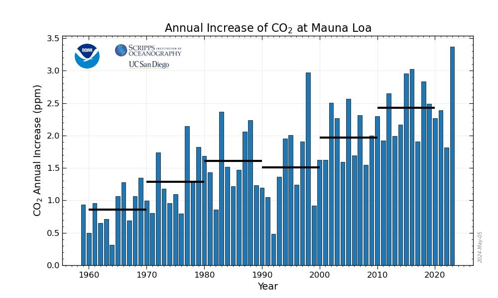
dCO2/dt has a very important physical meaning – it is the (annual for example) change in atmospheric CO2. It represents the sum of all CO2 added to, and removed from the atmosphere over a time period by human activities and by natural (non-human) processes. It’s the net CO2 emission.
This net emission looks very similar to the global temperature anomaly (to the human emission not nearly as much) and that is very remarkable. You only need the temperature anomaly to calculate the net emission! Human emissions seem to be irrelevant. Again, very remarkable! The sum of human and natural emissions depends on only one variable – the temperature anomaly.
According to the consensus, without human emissions, the natural emission would be basically zero. With human emissions, the natural emissions are obviously not zero anymore, but negative and in average about half of the human emissions. So, natural emissions depend on the human emissions.
I think the assumption that without human emissions, natural emissions are zero, is wrong. The seasonal CO2 cycle does not balance out (why would it?) and there is an annual residual. The residual is not random but depends on the temperature anomaly. It’s not the temperature anomaly as such causing the residual, but something related to it. Annual temperature cycle, sea ice cycle…
Gotta go..
Actually, there is firm physical ground, if PERSISTENTLY warmer than average temperatures produce increasingly higher CO2 concentrations, which they do. The devil lurks not in that basic concept of natural relationship, but in the tacit exclusion of all other sources of CO2. From all indications, they can overwhelm the natural temperature-driven CO2 variations, while being incoherent with temperature.
edimbukvarevic,
The problem is in the attribution of what part of dCO2/dt is emissions caused and what is temperature dependent.
You have two variables influencing CO2 and thus dCO2/dt: one is temperature with a small trend and a lot of variability, the other are human emissions with a huge trend and very little variability.
If you take the derivative of CO2, then you remove almost all of the trend and what remains is a small trend with a lot of noise. Everybody in this world, skeptics and warmistas alike, agrees that the CO2 rate of change variability is caused by the temperature variability (BTW the variability in dT/dt is exactly the same). Where the discussion is, is if the trend over time in dCO2/dt is mainly caused by temperature (Bart, Dr. Salby), or mainly by human emissions (many others: all warmistas but also many skeptics).
If you integrate T over time, you implicitely assume that all CO2 increase is temperature induced. If you integrate dT/dt over time, you have a few ppmv extra CO2 (16 ppmv/K as per Henry’s law), the rest is from the twice as high emissions.
Opposite, if you compare the observed dCO2/dt with the temperature variability at one side and the combination of temperature variability (4 ppmv/K) and human emissions effect (emissions – net sink rate per Henry’s law) on the other side, you see exactly the same result, down
to the deepest detail:
http://www.ferdinand-engelbeen.be/klimaat/klim_img/rss_co2_emiss_2000-2015.jpg
Where:
dCO2/dt(obs) is the observed dCO2/dt
RSS_CO2 is the CO2 rate of change based on the RSS temperature * factor + offset
emiss-deriv is the derivative of human emissions
emiss-CO2-deriv is the calculated derivative of the emissions minus the calculated net sink rate
emiss-nat-CO2-deriv is the previous plus the variability caused by the temperature variability
The three trends match exactly: the RSS trend due to the factor and offset, the emiss-nat-CO2-deriv trend with no further factor or offset.
Problem: which one is right?
Human emissions as cause is consistent with all observations:
http://www.ferdinand-engelbeen.be/klimaat/co2_origin.html
Temperature as main/sole cause with none…
1sky1,
See my previous reaction to edimbukvarevic.
In general:
If you have a process which is fed with a constant flow of some material and which is temperature dependent (like a cement oven), you will have a constant outflow of CO2 as there is no feedback. More (or faster) with higher temperatures.
Take the ocean upwelling: a constant input of cold, CO2 laden waters upwelling from the deep, warmed to ~30°C, which increases the internal CO2 pressure (pCO2) to ~750 μatm. As the atmosphere is at ~400 μatm, the ~350 μatm pCO2 difference pushes some 40 GtC/year as CO2 into the atmosphere.
As long as the same in reverse order happens near the poles, everything is in steady state.
Now the oceans at the upwelling area is heating up with 1°C. That increases the pCO2 of the upwelling waters with ~16 μatm. Thus pCO2(aq) increased from ~750 μatm to ~766 μatm. As the exchange flux is directly proportional to the the pCO2 difference with the atmosphere now pushes 41.8 GtC/year into the atmosphere. As the temperature at the sinks didn’t change, there is a disequilibrium: 1.8 GtC/year (~0.9 ppmv/year) CO2 increase in the atmosphere.
According to Dr. Salby and Bart, that extra inflow remains the same, as long as the temperature offset remains the same.
In the real world there is a negative feedback: the extra CO2 entering the atmosphere increases the pCO2 of the atmosphere, thus reduces the pCO2 difference between waters and atmosphere and increases the pCO2 difference at the sink areas. When the increase in the atmosphere is ~8 ppmv, the pCO2 difference at the upwelling then gets ~758 μatm, reducing the CO2 influx to ~40.9 GtC/year, while at the sink side the extra 8 μatm pushes ~40.9 GtC/year back into the deep oceans.
The negative feedback by the increased CO2 pressure makes that the initial extra CO2 input is reduced to a value where inputs and outputs are again the same as before the temperature increase. In this case ~8 ppmv extra in the atmosphere for an average ocean surface temperature increase of ~0.5°C
Bart’s formula then gets:
dCO2/dt = k(T-T0) – k2*[pCO2(t) – pCO2(0)]
At the moment that the new steady state is reached, dCO2/dt = 0 and
pCO2(t) – pCO2(0) = k/k2*(T-T0)
where k/k2 ~ 16 ppmv/°C
The same 16 ppmv/°C for the full dynamics of the world wide oceans as for a single static lab sample per Henry’s law…
Bart doesn’t (want to?) understand that this is a fully dynamic process, including inputs, outputs and feedbacks, where the processes act differently to temperature than to pressure changes…
A pressure change feedback which is completely absent, both in Bart’s and Dr. Salby’s temperature-only formulas…
Ferdinand,
Most of it seem to be temperature dependent since we started measuring:
dCO2/dt = k*Ta
Your reply does not make much sense. Small trend, huge trend?
edimbukvarevic,
The trend of temperature since 1958 until now is 0.8°C with a variability of +/- 0.4°C or about 50% of the trend.
The CO2 trend is 90 ppmv with a year to year variability of +/- 1.5 ppmv around the trend or max. 2% of the trend.
The CO2 emissions trend over the same time span were ~155 ppmv with a year to year variability of only +/- 0.2 ppmv or about 0.1% of the trend.
If we may assume that Henry’s law still is at work, then an increase of 0.8°C is good for maximum ~13 ppmv increase in the atmosphere, no matter if you shake a small sample of seawater or the whole oceans. The short term variability then is good for maximum +/- 3.5 ppmv. As the variability fades out within 1-3 years, the extremes (Pinatubo, El Niño) only reach +/- 1.5 ppmv before the temperature goes back in the other direction. That is visible in the lagged response of CO2 to the extremes in temperature around the trend:
http://www.ferdinand-engelbeen.be/klimaat/klim_img/wft_trends_rss_1985-2000.jpg
A variability of half the temperature trend has 1.5 ppmv effect, the full temperature trend would give 90 ppmv? Not only is that very unlikely as the CO2 response to temperature is very fast (less than a year) but it violates Henry’s law for the solubility of CO2 in seawater…
Moreover, most of the variability is the result of temperature variability on (tropical) vegetation, but vegetation is a net, growing sink for CO2, thus not the cause of the increase of CO2 in the atmosphere…
That vegetation is the cause of the variability can be seen in the opposite changes in CO2 and δ13C. If the oceans were the main reactant, then CO2 and δ13C changes would parallel each other.
Here for the derivatives:
http://www.ferdinand-engelbeen.be/klimaat/klim_img/temp_dco2_d13C_mlo.jpg
If you look at the temperature derivative, you can see that it has the same variability as in T and dCO2/dt, but zero trend, only a small offset from zero. If you integrate dT/dt, then you will find back the small CO2 increase as per Henry’s law.
Integrating T gives you a non-physical answer as that is partly based on a real correlation (the variability), but a spurious trend, which in dCO2/dt is not caused by temperature…
What Ferdinand does not understand is that every layer of the ocean is just like the atmospheric/oceanic interface. Once you equilibrate the pCO2 between the atmosphere and the surface layer of the ocean, you now have to equilibrate the pCO2 between the surface layer of the ocean and the next one down. And, then the next one, and the next one, and so on down in an ocean that runs deeper in some places than the tallest mountains are high.
That equilibrium does not happen overnight. It takes a long time. And, that is what gives rise to an apparent proportionality of the rate of change of CO2 to temperature anomaly. Ferdinand is treating the vast oceans as though they were a shallow pond. It is ridiculous.
Ferdinand has nothing to prove me wrong, just a misplaced faith in a particular interpretation of unverifiable and poorly resolved ice core proxies that he insists must be better than the far more accurate, direct measurements taken since 1958. Without that, he has no case at all. It is an edifice whose foundation rests on quicksand, as will become apparent with the next extended cooling (or at least non-warming) cycle.
“dCO2/dt = k(T-T0) – k2*[pCO2(t) – pCO2(0)]”
Were this true, the same process would apply to anthropogenic inputs, and they also would have no significant impact. Ferdinand only gets a vague resemblance between the data and his model by A) illegitimately decoupling the anthropogenic dynamics from the natural ones, B) assuming that the phenomenal match between the long term trend in dCO2/dt and T is just a staggering coincidence, which he can arbitrarily filter away.
“A pressure change feedback which is completely absent, both in Bart’s and Dr. Salby’s temperature-only formulas…”
It isn’t. It is readily apparent in my formula before simplifying it. It has negligible impact – we actually both agree on that – and that is why it does not appear in the final approximation. Ferdinand is ignoring the long term equilibrium dynamics that do have a significant impact.
Ferdinand,
While I concur that anthropogenic CO2 emissions are not incorporated into Salby’s model, the matter of “feedback” of CO2 upon ocean temperatures, in particular, is quite dubious. It’s recognized by the most sophisticated analysts that the dependence of global temperatures upon CO2 is very difficult to quantify empirically in terms of a power transfer function (see, e.g., http://www.pnas.org/content/94/16/8370.full.pdf), because of the high uncertainty in spectral estimation from short records. (Unfortunately, despite his analytic sophistication, Thompson fails to recognize the high bias of the global temperature record he employs.)Nonetheless, your implicit belief that predominantly anthropogenic CO2 variations exert a STRONG feedback effect upon T is simply inconsistent with the results of cross-spectrum analysis of vetted modern records.
P.S. This is not a acceptable venue for displaying the research underlying my cautionary remarks.
Bart:
every layer of the ocean is just like the atmospheric/oceanic interface.
Bart, you are completely mistaken on this. The uper ocean layer, the “mixed layer” is very responsive to changes in the atmosphere and reverse, as the exchange between them is very intensive by wind and waves, which mixing rates bypassing the extremely slow diffusion rate of CO2 in seawater.
Except for the intensive biological pump, there is hardly any migration of CO2 between the surface layer and the next layer(s), as good as there is hardly any temperature exchange between the top layer and the next layer(s).
The main direct exchanges of water, temperature, CO2 and other elements from surface to deep oceans are via the sink and upwelling zones (each about 5% of the ocean surface area). That water cycle needs ~800 years to return to the surface.
That means that short term variability (seasons to centuries) are hardly influenced by the deep ocean exchanges and if they change (temperature, CO2 concentration,…) then these changes are rapidly met by the fast response in the atmosphere.
E.g. if there would be a sudden extreme increase of 10% CO2 (and derivatives) in the upwelling waters, that will give a sudden increase of 20% in the CO2 influx at the upwelling for the same temperature. That gives an increase of CO2 in the atmosphere, which reduces the input and enhances the output. The initial increase in input of 20% ultimately gets 12.5% while the output is enhanced with 12.5%, thus back to steady state. The CO2 increase in the atmosphere thereby gets ~30 ppmv higher:
http://www.ferdinand-engelbeen.be/klimaat/klim_img/upwelling_incr.jpg
A 10% increase in concentration is a practical impossibility, as the enormous reservoir dampens such variability…
Thus indeed the main exchanges are mainly between the “shallow” ocean surface and the atmosphere, which doesn’t imply that the exchanges are static, they still are very dynamic (seasonal) and with the deep oceans for CO2 still (slower) dynamic…
Were this true, the same process would apply to anthropogenic inputs, and they also would have no significant impact.
The same process applies to anthro inputs as to volcanic inputs. In the formula:
dCO2/dt = k(T-T0) – k2*[pCO2(t) – pCO2(0)]
k2 = ~0.02, thus for T = T0 and pCO2(t) = 400 ppmv and pCO2(0) the steady state at ~290 ppmv, dCO2/dt = 2.2 ppmv/year, the current average net sink rate.
For all pre-industrial volcanic inputs at 0.1 ppmv/year, the equilibrium would be at 0.1 / 0.02 = 5 ppmv extra in the atmosphere…
At steady state the natural inputs at one side with a local ΔpCO2 of 350 μatm are fully compensated with the outputs at a local ΔpCO2 of 250 μatm at the sink side.
Before responding: k2 is the observed overall global coefficient for the influence of pressure changes in the atmosphere above steady state, highly linear over the past near 60 years. That is not the same constant that governs the flux as result of the local ΔpCO2 between atmosphere and oceans at the source and sink areas. The latter are governed by temperature and Henry’s law. k2 is for the influence of a change of CO2 in the atmosphere on the local ΔpCO2 at sources and sinks.
Thus:
A) illegitimately decoupling the anthropogenic dynamics from the natural ones
Is completely legimate for the decoupling of upwelling and sinks with direct injections into the atmosphere, as the former are driven by temperature differences and hardly influenced by pressure changes, while the removal of any extra CO2 in the atmosphere is only possible by the influence of pressure changes on sources and sinks… Different responses of the same processes to temperature and pressure changes.
B) assuming that the phenomenal match between the long term trend in dCO2/dt and T is just a staggering coincidence
Pure nonsense: the match in trend is not fenomenal and in 35 of the 57 years even negative. You can match the amplitudes or the slopes, not both.
Moreover, as variability and trend are (proven!) caused by different processes, there is no reason at all that the same factor applies to both neither that temperature has any influence on the trend.
Further, while near all of the variability is caused by temperature variability, almost all of the trend is caused by the twice as high trend in human emissions. The integral is not between T and dCO2/dt, the integral is between dT/dt and dCO2/dt, where dT/dt has no trend and all variability.
You have zero evidence that the trend in dCO2/dt is caused by temperature.
It is readily apparent in my formula before simplifying it. It has negligible impact – we actually both agree on that –
What? I never “agreed” on a lack of impact of an increased CO2 pressure in the atmosphere. We agreed on a lack of short time impact of the deep oceans, as far as I remember, but that has nothing to do with the impact of the increased CO2 levels in the atmosphere on the CO2 in/out exchanges with the deep oceans.
And please, don’t put words in my mouth that I never spoke or implied: CO2 levels in ice cores are quite accurate, but show a long (10 to 600) years average of the historical levels. Since 1958 we have very accurate and even hourly data…
1sky1,
I think that you misunderstand my position:
While I am a firm defender of the human cause of increased CO2 levels in the atmosphere, I am an equal firm defender of the lack of (catastrophic) impact of the extra CO2 on climate…
In my opinion, more CO2 has a modest impact on temperature (1-1.5 K for 2xCO2), which is beneficial in many ways, including the impact of more CO2 itself on plant growth, with very few negative impacts.
And I don’t think that current climate models have any value beyond scaring people with results that have nothing to do with what happens or will happen in the real world…
Ferdinand:
Alas, even the “modest” impact of increased CO2 upon GAST that you cite is based upon little more than simplistic, back-of-the-envelope calculations of “climate sensitivity,” incorporating misguided notions of what constitutes feedback in physically realizable systems. Requisite understanding of ADAPTIVE nonlinear system behavior is virtually nonexistent in “climate science.”
You’re just spinning a yarn, Ferdinand.
“Is completely legimate for the decoupling of upwelling and sinks with direct injections into the atmosphere.”
It is not. When a balance is struck between competing forces, you cannot change that balance by proportionately more than your proportionate influence. You quite simply cannot. It is not up for negotiation.
“Pure nonsense: the match in trend is not fenomenal and in 35 of the 57 years even negative.”
Nonsense. Cherry picking short intervals is just looking at noise. You must know this is misdirection, and you should be ashamed of it.
“Further, while near all of the variability is caused by temperature variability, almost all of the trend is caused by the twice as high trend in human emissions.”
Mere assertion.
“The integral is not between T and dCO2/dt, the integral is between dT/dt and dCO2/dt, where dT/dt has no trend and all variability.”
You would have made a great monk, conjuring up epicycles to prove Galileo wrong.
“I never “agreed” on a lack of impact of an increased CO2 pressure in the atmosphere. “
You have repeatedly claimed that the short term effect via temperature related changes in Henry’s Law coefficient produces negligible increase. I agree. But, this is not the only temperature related change in the transport of CO2 within the ocean currents.
I think we’ve said all that can be said for now. Watch and see what happens.
“dCO2/dt = k(T-T0) – k2*[pCO2(t) – pCO2(0)]
k2 = ~0.02, thus for T = T0 and pCO2(t) = 400 ppmv and pCO2(0) the steady state at ~290 ppmv, dCO2/dt = 2.2 ppmv/year, the current average net sink rate.”
One last thing. What this says is that the current rate of natural emissions is k2*pCO2(0) = 5.8 ppmv/year equivalent. But, we know that human emissions are, at most, 5% of natural emissions, so that requires H be less than 0.29 ppmv/year equivalent. Yet, for 1/2 of all emissions to be the cause of the observed rise, they would have to be more than an order of magnitude greater than that.
This is why your model is illegitimate. The numbers do not line up because you have stacked the deck against the natural emissions.
@ Bartemis
May 15, 2017 at 1:32 pm; Thank you Bart. This ‘refutation’ has a strangeness to it, which is not new to me. Just saddening. But we are bigger than this….
Bartemis May 17, 2017 at 6:19 pm
“dCO2/dt = k(T-T0) – k2*[pCO2(t) – pCO2(0)]
k2 = ~0.02, thus for T = T0 and pCO2(t) = 400 ppmv and pCO2(0) the steady state at ~290 ppmv, dCO2/dt = 2.2 ppmv/year, the current average net sink rate.”
One last thing. What this says is that the current rate of natural emissions is k2*pCO2(0) = 5.8 ppmv/year equivalent. But, we know that human emissions are, at most, 5% of natural emissions, so that requires H be less than 0.29 ppmv/year equivalent. Yet, for 1/2 of all emissions to be the cause of the observed rise, they would have to be more than an order of magnitude greater than that.
Which of course they are! Current CO2 emissions from fossil fuel use are ~36 Gtonne CO2/yr which is ~4.7ppmv/yr.
Which shows Ferdinand’s model is wrong. Thank you.
Bartemis May 18, 2017 at 7:11 am
Which shows Ferdinand’s model is wrong. Thank you.
No it just shows that you don’t understand the difference between the net rate between sources and sinks and the source rate! Ferdinand shows that at today’s pCO2 the natural flux is a net -2.2ppmv/yr, which is consistent with the ff flux being 4.7ppmv/yr, therefore a net increase of ~2.5ppmv/yr.
No, it shows you don’t understand the model. If the FF flux is 4.7 ppmv/yr, then the natural flux has to be at least 20X that.
I.e., You must have k2*pCO2(0) greater than 4.7*20 = 94. If pCO2(0) = 280, then you must have k2 greater than 94/280 = 0.34, which indicates a time constant of less than 3 years. There is no way one can make the budget close with a time constant of 3 years.
Bartemis May 18, 2017 at 8:10 am
No, it shows you don’t understand the model. If the FF flux is 4.7 ppmv/yr, then the natural flux has to be at least 20X that.
Which the flux from natural sources is, but it’s slightly less than the flux into the sinks giving the -2.2ppmv/yr referred to above.
It isn’t in Ferdinand’s model. It is only 5.8 ppmv/year equivalent, a factor of 1.2X, not something north of 20X, as it should be if the model were even to be a contender.
Bartemis May 18, 2017 at 9:00 am
It isn’t in Ferdinand’s model. It is only 5.8 ppmv/year equivalent, a factor of 1.2X, not something north of 20X, as it should be if the model were even to be a contender.
As I told you before that is the net flux (source-sink).
This diagram of the fast carbon cycle shows the movement of carbon between land, atmosphere, and oceans. Yellow numbers are natural fluxes, and red are human contributions in gigatons of carbon per year. White numbers indicate stored carbon. (Diagram adapted from U.S. DOE, Biological and Environmental Research Information System.)
Sorry, no. That is an illegitimate decoupling of the natural and anthropogenic flows. The natural flows must add at least 20X (more likely 30X or more) of the anthropogenic flows in order for it to be a physically viable model.
You can make any assertions you like until you are blue in the face. I am under no obligation to accept them, especially when they are physically untenable.
Bartemis May 18, 2017 at 12:44 pm
Sorry, no. That is an illegitimate decoupling of the natural and anthropogenic flows. The natural flows must add at least 20X (more likely 30X or more) of the anthropogenic flows in order for it to be a physically viable model.
Only if you ignore the sinks!
You can make any assertions you like until you are blue in the face. I am under no obligation to accept them, especially when they are physically untenable.
No, but by taking that point of view you reveal your total lack of understanding of the system.
Phil. you’d have more luck arguing with a brick wall. At least a brick wall understands what a sledgehammer is.
Sorry, no. The lack of understanding is totally on your part.
In the model equation, the term k2*pCO2(0) represents the natural sources, the k2*pCO2(t) term the sinks. Combined together, they represent the net. But, each term must individually fulfill its role.
The term k2*pCO2(0) must be at least 20X, more likely 30X or more, of the human contribution, to be physically tenable. There is no way around that. Anthropogenic sources are a small percentage of natural sources.
If Ferdinand adjusts his k2 to fulfill this requirement, he will blow his model to smithereens. It will no longer even superficially reproduce what is seen in the observations.
Bartemis May 18, 2017 at 1:50 pm
Sorry, no. The lack of understanding is totally on your part.
In the model equation, the term k2*pCO2(0) represents the natural sources, the k2*pCO2(t) term the sinks. Combined together, they represent the net. But, each term must individually fulfill its role.
You’re mistaken, as Ferdinand clearly states k2*pCO2(t) is the net flux in state t (in this case at T=T0 and [CO2]=400ppmv) and k2*pCO2(0) is the net flux in the reference state ( T=T0 and [CO2]=290ppmv)
The term k2*pCO2(0) must be at least 20X, more likely 30X or more, of the human contribution, to be physically tenable. There is no way around that. Anthropogenic sources are a small percentage of natural sources.
This is not true, due to your misunderstanding of what the terms mean.
If Ferdinand adjusts his k2 to fulfill this requirement, he will blow his model to smithereens. It will no longer even superficially reproduce what is seen in the observations.
No such adjustment is necessary as indicated above.
You are confused. It is as I have explained it to you. These terms represent natural additions and subtractions from the rate of change.
Bart:
The term k2*pCO2(0) must be at least 20X, more likely 30X or more, of the human contribution, to be physically tenable.
Which only shows that you have no idea how the natural cycles work.
You treat all CO2 cycles as one (temperature controlled) process. That is where it gets wrong even before you start:
1. Sinks don’t depend of the sources of one year, they mainly depend on local temperature and somewhat on global CO2 pressure in the atmosphere.
2. Temperature changes/differences are the main drivers of almost all natural in/out fluxes:
A) ~50 GtC out/in per season oceans.
B) ~60 GtC in/out per season biosphere.
C) ~40 GtC/year continuous out and continuous in between warm upwelling and cold sinks
Total fluxes ~150 GtC/year flowing between different reservoirs.
Current balance of all these fluxes in the atmosphere: ~800 GtC reservoir + 4.5 GtC/year +/- 3 GtC natural variability.
Global seasonal variability over a year: +/- 10 GtC
Global residual variability over a year: +/- 3 GtC
Total natural variability over a year: +/- 13 GtC
Observed residual increase/year: +4.5 GtC
At no moment in time there is 150 GtC extra in the atmosphere, the net effect of A) and B) is not more than +/- 10 GtC amplitude as these are countercurrent, which near zeroes out after a full cycle.
The net effect of C is zero, as long as ins and outs are equal.
Thus of all natural fluxes, the net effect in the atmosphere at any moment is maximum +13 GtC (in winter) and minimum -13 GtC (in summer), incuding the natural year by year variability of all these fluxes together.
Human emissions are +9 GtC/year. That is of the same order as what the natural fluxes have at their peak moment in the atmosphere, but a lot higher than the natural fluxes at their lowest values. In average the natural fluxes are -4.5 +/- 3 GtC/year.
Your problem is that you compare human emissions with the sum of all inputs together, which is never present in the atmosphere and thus can’t influence the sinks, while you should compare human emissions with the net balance of all cycles at every moment.
Human emissions disturb the balance between inputs and outputs of the natural cycles into more sink that source and the net result is an increase in the atmosphere.
Ferdinand – I have given you a hard mathematical requirement. You have given me your usual plate of assertions.
I’m sorry. Your model is physically invalid. You have illegitimately elevated anthropogenic emissions over natural ones.
There is no defense, and you are just waving your hands and blustering.
Bartemis May 18, 2017 at 2:26 pm
You are confused. It is as I have explained it to you. These terms represent natural additions and subtractions from the rate of change.
The confusion is all yours, read it again.
No, Phil. You are digging in your heels, but you haven’t got a leg to stand on. You are absolutely wrong on a very elementary level.
You do not know either of us, and you have no idea what you are talking about. Run along.
Your viewpoint is that of a child. You have no means of discerning scientific truth.
This is not a close call. Phil has made an elementary mistake. Almost as bad as the pseudo-mass balance argument.
No, I take that back. It’s a pretty basic mistake. They are on a par.
“You are digging in your heels, but you haven’t got a leg to stand on.”
???
[The mods note that use of the pejorative “digging in heels” implies, even demands, the presence of both legs and both heels; but it also indicates that both the “diggee” and “digger” have opposing ideas that must be equal and balanced, or the heel-digger would immediately fall backwards onto his or her own fleshy invectives. .mod]
You guys are a riot. I’d love to stay and chat some more, but there are things to do…
“since since” should just read “since”…
Fonzie – further response here.
The pseudo-mass balance argument only tells us what the flux is in the presence of anthropogenic inputs. It does not tell us what nature is doing on its own. It fails because outputs are a function of inputs, and change if anthropogenic inputs are removed.
EG – hate to be the one to inform you, as your parents really should have told you at some point. But, Santa Claus and the Easter Bunny are not real, and have no substance. Ergo, the comparison with the pseudo-mass balance argument is apt. Anyone who believes in any of the above should voluntarily commit themselves to a home where they take care of people like that.
” The logical result is that the yearly rise in CO2 is not from natural sources, because the natural sinks cannot keep up with human emissions.”
That is an intuitive result, not a logical one. Intuition told us the Sun revolved around the Earth. Intuition told us that drought meant the gods were angry. Intuition told us time was absolutely uniform throughout the universe.
Intuition is a poor substitute for science.
This is all about sink rates, EG. If the sinks are powerful enough, then all but a small fraction of CO2 additions are removed, from natural or anthropogenic sources. But, the natural sources are much more powerful than anthropogenic sources, on the order of 30X or more. Hence, the residual that remains is at least 97% natural, and 3% anthropogenic.
It all works out in the math, EG, though you do not understand the math. You are in way over your head, and you should just bow out.
Sure… By using the word “could”, i wasn’t trying to be definitive. Ferdinand got into trouble with the very same word (“could”) in the comment section of his 2010 piece on the mass balance argument. (in an almost identical situation, he used ice core data as opposed to your use of isotope data here) Much jocularity among the commentors that english was not his native tongue. So after reading that fiasco, i always deliberately use the non definitive “could” as opposed to the definitive “would”. Other arguments may well prove that the rise is anthropogenic (though the mass balance argument does not)…
Not even close, young one. 14C has been all out of whack since the atomic era began. As a result, it is completely useless for attribution studies to the present time. That’s why your link is talking about the future.
Some advice: read your links before passing them around.
“which is in the table at the bottom of the link I provided”
Look again. Those are tables of results of computer simulations.
That’s three strikes in a row, kid. Do you ever get tired of being wrong?
And a lot of other local things like rainfall, wind etc.. That’s why the correlation is damning.
Nope. It is local in time.
So in reflection we have had a lot of defenses of the undefendable…
Humans emit ~9 GtC/year as CO2, only from fossile fuel burning + land use changes, not included.
The increase in the atmosphere is ~4.5 GtC/year, the rest is absorbed mainly by oceans and vegetation.
That humans are responsible for the increase in the atmosphere is consistent with all known observations.
Logic and observations says that we are fully responsible for most of the recent increase of CO2 in the atmosphere.
Then all hell breaks loose and a lot of people calling themselves “skeptics” refute logic and come with 1001 “alternatives” or simply believe unskeptical anyone or any article that shows that maybe there are non-human alternative explanations for the CO2 increase in the atmosphere. As that is one of the main fundaments of the AGW hypothese, it MUST be wrong…
Problem with all these alternatives is that they all, from the first to the last, fail one or more observations.
Bart’s hypothesis has the record: it fails every observation (except some arbitrary curve “fitting” of two straight lines)). Congratulations!
New defence line: the observations must be wrong.
Sorry boys (and girls) a little more critical thinking about your own pet theory and/or what fellow “skeptics” say would be good for the skeptics case. That humans are NOT responsible for most of the CO2 increase in the atmosphere is just shooting in your own foot and divert the attention from where the real battle is: the real effect of more CO2 on temperature and climate with a lot of benefits and few drawbacks…
“Logic and observations says that we are fully responsible for most of the recent increase of CO2 in the atmosphere.”
You are not using logic. You are using intuition. And, intuition is a notoriously poor means of discerning scientific truth.
My hypothesis fits every observation, just not necessarily your interpretation of a given observation. Yours fails fundamental physical constraints.
There really is no doubt about it. You will see.
Bart:
My hypothesis fits every observation
Name one (curve fitting with an arbitrary offset and factor is not an observation)…
Ferdinand:
The offset and scaling factor merely compensate for the arbitrary temperature anomaly baseline, and the units conversion between the quantities. They do not impact the fundamental fingerprint that establishes the temperature dependence of the rate of change of CO2. That fingerprint consists of: A) the match between the variability of each time series, B) the match between the long term trend in each time series.
The data irrefutably show that the only physically viable dynamic is approximately
dCO2/dt = k*(T – T0)
The only way you can claim otherwise is to dismiss the extraordinary match between the long term trends, and arbitrarily filter it out, producing a model which treats natural inputs and anthropogenic inputs on separate playing fields, which is physically verboten.
Your interpretations of other observations are not unique explanations. There is room for alternative explanations. You need to seek out those alternatives. Because there is no alternative to the above.
Bart,
Do you have any single observation in the real world, besides the match of two slopes, that supports your theory?
That’s all that’s needed, Ferdinand. It is a unique explanation. There is no physically viable alternative.
All your other “evidences” are just a mishmash of biased inference with alternative interpretations. Meaningless. This one cannot be gainsaid.
“…curve fitting with an arbitrary offset and factor…”
Ferdinand, it’s not as though we’re fitting the keeling curve to gisstemp here. The MLO data only goes back to 1958, so a proper offset is not available to us. And scaling the two curves to one another (unlike keeling and giss) provides a near perfect fit; the two curves actually look alike… What more can be expected of the “derivative plot”?
Bart and Fonzie,
There is simply no connection between most of the variability and most of the trend.
Most of the variability is caused by the reaction of (tropical) vegetation on temperature variability.
The trend is NOT caused vegetation.
Although I know that you don’t accept any observation that rejects your theory, that the variability is mostly caused by vegetation is based on the opposite CO2 and δ13C changes. On the other side, vegetation is a proven sink for CO2, thus not the cause of the trend.
As proof of the disconnection between the variability and trend, that is as solid as adding an acid to a solution and expecting that the pH gets lower.
Thus all the “fit” you have is between variabilities. You have zero evidence that the trend in CO2 rate of change has anything to do with the trend in temperature…
You have zero evidence that it does not. And, a tortured alternative explanation worthy of the epicycles of the monks of the 16th century.
Bart,
You have zero evidence that it does not.
Bart, the opposite CO2 and δ13C changes are full proof that the CO2 changes are mainly in vegetation
The oxygen balance and observations of growing biomass are full proof that vegetation is not the cause of the trend.
That doesn’t exclude temperature as cause of the trend, as oceans may be the source (they aren’t), but it proves that variability and trend are caused by different processes. Thus your “one temperature process fits all” is on shaky grounds (epicycles where?)…
” Thus all the “fit” you have is between variabilities. ”
Ah! But the “fit” is also between the trends, as both the variabilty features AND the trend features fit. (one can just as easily lay claim to the fit between trends as the fit between variabilities)…
“… the opposite CO2 and δ13C changes are full proof that the CO2 changes are mainly in vegetation”
No, they aren’t. There is much we do not know about isotopic compositions from the various sources. Furthermore, there is a dilution effect. If you have our usual kitchen sink with the faucet on, and you supplement the flow with a small percentage of blue dye, the water is going to take on a blue tinge, even though the dye input is barely budging the level.
“The oxygen balance and observations of growing biomass are full proof that vegetation is not the cause of the trend.”
This, again, is an expression of certainty regarding flows that is just not valid.
These are rationalizations, not evidences.
Bart,
There is much we do not know about isotopic compositions from the various sources.
What we do know about isotopic compositions of the different sources is more than sufficient to know that (tropical) vegetation is the main reactant on temperature changes.
And there is a double check that vegetation is not the cause of the CO2 trend, it is a growing sink for CO2.
It is not because you don’t like the result, that it isn’t rock solid proven…
“What we do know about isotopic compositions of the different sources is more than sufficient to know that (tropical) vegetation is the main reactant on temperature changes.”
Nope. The data fit
dCO2/dt = k*(T – T0)
and you do not have a physically viable alternative.
Fonzie,
The effect of the variabilities in dCO2/dt gets +/- 1.5 ppmv around the 90 ppmv trend.
The variabilities in T are up to half the total trend in T over the past near 60 years:
http://www.ferdinand-engelbeen.be/klimaat/klim_img/temp_co2_1960_cur.jpg
The transient response of CO2 to T changes is less than a year and 4-5 ppmv/K
The equilibrium response of CO2 to a sustained T change would take some 4-5 years and maximum 16 ppmv/K (there we have the good old Henry again…).
Today I read a very interesting paper unknown to me till now:
http://www.pnas.org/content/94/16/8370.full.pdf
Dependence of global temperatures on atmospheric CO2 and solar irradiance
David J. Thomson (Bell Labs), 1997
(presented at a colloquium entitled ‘‘Carbon Dioxide and Climate Change,’’ organized by Charles D.
Keeling, held Nov. 13–15, 1995, at the National Academy of Sciences, Irvine, CA.)
Apart from his amazing accuracy in getting rid of numerous biases in trend computations still ignored by many today’s scientists, one impressive result in the paper was that he discovered (in 1994!)
« Analysis of the low-frequency and annual parts of the temperature records yield at least three largely independent indicators of climate change
– the change in distribution of individual station phase trends about the mean, the change in average phase
– and the increase in average temperature. »
This is exactly what we actually experience in the polar regions, where sea ice extent anomaly plots for the recent years look as if the annual cycles hadn’t been removed out of their originating time series.
What an interesting lecture for a layman!
The same discussion between Ferdinand and Bartemis took place years ago here:
http://notrickszone.com/2013/10/08/carbon-dioxide-and-the-ocean-temperature-is-driving-co2-and-not-vice-versa/
A never ending process, as it seems…
Yes, it has been going on even longer than that. I’m not sure I could put a precise date on it, but I think it is over a decade.
And, throughout that time, the relationship between the rate of change of atmospheric CO2 and temperature has remained true. The rate settled out with the “pause” in temperature anomaly while emissions kept accelerating onward and upward.
http://i1136.photobucket.com/albums/n488/Bartemis/scale%200.22_zpsq4jxp1xy.png
http://cdiac.ornl.gov/images/global_fossil_carbon_emissions_google_chart.jpg
It tracked the El Nino blip we just went through. And, it is now falling rapidly in sync with the current plunge in temperature anomaly.
With luck (of a sort), we will soon reconverge to the ~30 year downcycle, of the ~60 year periodic component evident in the temperature records, that was delayed in appearance by the monster El Nino. When the curve decelerates in sync, we will hopefully have proof positive that nobody can deny any longer.
Bindidon,
Yes, the same discussion bursts out every few months since several years… Until some sudden cooling event would show up that shows one of us is right…
“Until some sudden cooling event would show up that shows one of us is right…”
And on that day, ferdinand, we’re gonna serve you up a great big plate of crow! (with a nice big slice of humble pie for dessert!)…
All kidding aside, it would really be a shame to wait five years or so for that to happen. Such a discussion should begin now. (or at least every effort should be made to get there sooner) It would be a shame to see great talents wasted on an argument that’s going nowhere. It’s not unheard of to assume something that you think wrong is right, just to advance knowledge and understanding. And if that doesn’t happen, i hope one of y’all can break the stalemate so that you don’t have to wait five more years. (that’s how long it will take to wade through ferdinand’s interannual variability) Life is short…
Mod – my reply here seems to have disappeared into the ether. Can you please see if you can rescue it? Thx…
Trophobiosis
Hydrocarbons upwell from deep underground until they reach a strata
of soil we call topsoil. Aerobic microbes extend into the soil to the
depth oxygen can penetrate. These microbes use the oxygen and
hydrocarbons to oxidize the hydrocarbons, excrete CO2 and fertilize
the soil in their life cycle. The fertile soil and the CO2 allow the
plant, in the presence of sunlight, to perform photosynthesis. As the
plant grows, this process produces oxygen, which feeds the microbes.
The above described process means that local CO2, at ground level,
can be a very much higher in areas which have very rich soil, such
as Kansas or the Ukraine. This extra CO2 means that lower growing
plants in these areas are not dependent on limited CO2 levels elsewhere.
As long as topsoil anywhere has access to oxygen, plants growing in
that soil will not starve for CO2.
On my property, in a separation of 1500 feet, the amount of upwelling
hydrocarbons vary by a factor of 2.
The exact amount of CO2 emitted by the microbes is unknown and would
require an amount of effort to survey which I cannot comprehend.
The fact that I have seen no indication of an attempt quantify this
source of CO2 means most, if not all carbon balance models, are at
best, SWAGS and probably WAGS.
The foregoing is the result of my research, not theories.
Nope. Fossil [hydrocarbons] never emerge from the surface; (Green River); they emerge from kerogen strata buried deep enough to be in the temp/pressure ‘oil window’ of catiagenesis. . Hydrocarbons upwell [until] stratigraphically capped by some impervious cap rock like a salt dome or Kern River caliche. Else no conventional oil reservoir forms from an underlying source rock shale. Like the giant ‘oil spill’ known as Athabascan tar sands.
JH, you need to study a lot more petroleum geophysics before commenting again.
Rud, my challenge stands. Lets do a real test, No bluster or theories.
A real test.
As a parting post, please everyone note that atmospheric concentration has been at a steady rate of about 2 ppmv/year ever since the “pause” began:
http://i1136.photobucket.com/albums/n488/Bartemis/scale%200.22_zpsq4jxp1xy.png
Total FF emissions just keep right on accelerating:
http://cdiac.ornl.gov/images/global_fossil_carbon_emissions_google_chart.jpg
Indeed, there is a marked acceleration in emissions about 2000, just at the time concentration suddenly decelerated.
Ask yourself, why? Is this consistent with emissions being the driving force behind atmospheric concentration?
No, it is not. After the latest El Nino, temperatures are plunging fast. The “pause” has been reinstated, and may continue indefinitely, or even transition into a cooling era. As emissions keep on accelerating, and concentration at most remains at essentially constant rate, it should not be too much longer before the discrepancy is too great even for the diehards to defend.
Please note that, in the above plot of the rate of change of concentration, the units are ppmv/month. A rate of 2 ppmv/year is 0.17 ppmv/month.
Bart you are ridiculous. If the “pause” persists for 1000 years, and CO2 continues to rise at 2 ppm/yr, then 1000 years from now, global temperature will remain the same but CO2 will be at 2400 ppm. Your “theory” doesn’t work.
You are one dumb kid.
Darby, by the time 1000 years would go by, a new equibrium state temp would have been reached and the carbon growth rate would be zero. (bart has explained this over and over and over again) Please pull your head out of your backside before you comment, it’s painful watching you embarrass yourself…
Michael is right, as there is zero feedback in Bart’s formula. Thus no matter how much CO2 enters the atmosphere, there is no feedback from the increased CO2 pressure in the atmosphere on the influxes and outfluxes from the oceans and vegetation.
Despite that vegetation is an observed, growing sink for CO2, thanks to the increased CO2 pressure in the atmosphere.
Despite that the oceans are an observed, growing sink for CO2, thanks to the increased CO2 pressure in the atmosphere.
Zero influence of these growing sinks on the increase of CO2 in the atmosphere: in Bart’s (and Dr. Salby’s) formula, the net influx remains exactly the same for a fixed temperature offset, despite a 30% (90 ppmv) increase of CO2 pressure in the atmosphere in less than 60 years (what will that be after 1000 years?)…
There is absolutely feedback in my model. You have now crossed the line into a lie.
Bart,
In you final formula, there is zero feedback from any increase of CO2 in the atmosphere. Even of that doubles or triples…
That is incorrect. The final formula has the “r” factor subsumed into the “k” factor, as I described here. That is the impact of the feedback you are talking about. It is all there. Just do the math.
Bart,
In your “toy model” you say:
Since r is small, the bulk of both the source H and the temperature constricted outflow k*T goes into the oceans. Suppose, e.g., that r = 0.01.
In the real world:
r := 10 for any change in the ocean surface as result of a change in the atmosphere (the “Revelle” factor).
r := 1 for the current distribution of CO2 from human emissions between atmosphere and deep oceans.
r := 0.01 for the ultimate distribution of all human emissions between atmosphere and deep oceans, but that has a response time of ~51 years for any CO2 pressure above steady state.
r depends of temperature, but that is mainly for the steady state between ocean surface layer and atmosphere. The exchanges with the deep oceans are hardly influenced by temperature changes.
Again what completely lacks in your formula is the response of r to pressure changes: that is where the real negative feedback is…
Ferdinand – after all these years, you have finally convinced me that you have absolutely no math skill whatsoever. I am tired of arguing about things you clearly do not understand. We’ll no doubt pick it all up at the same point next time. Until then, I’m done with this thread.
Bart,
My math skills are completely rusty, but that doesn’t mean that I don’t know what happens in the atmosphere-ocean exchanges, of which you haven’t the slightest idea.
In your formula, you use the ultimate distribution of human CO2 between atmosphere and deep oceans, which indeed is about 1:100.
What you did is applying the ultimate 1:100 distribution to the momentary distribution of human CO2, which doesn’t take into account the relaxation time needed to redistribute that extra CO2 in the atmosphere into the deep oceans…
The momentary distribution is about 1:10 ocean surface – atmosphere.
The momentary distribution is about 1:1 deep oceans – atmosphere.
The relaxation time is ~51 years.
Again, where is the response to an increased CO2 pressure in the atmosphere anywhere in your toy story?
Your math skills are nonexistent.
The response is in my model, from the beginning to the end. I did the math. I showed the math. You do not understand math. It’s hopeless.
Bart:
Your “math” is here:
Since r is small, the bulk of both the source H and the temperature constricted outflow k*T goes into the oceans. Suppose, e.g., that r = 0.01.
Translated into human language:
“Since r is small” means: I have no idea, but my model needs a small r.
“constricted outflow k*T” means: and then a miracle happens, but my model needs such miracle.
“Suppose, e.g., that r = 0.01” means: in the real world r = 1 to 10 (deep oceans – surface), but my model needs a much smaller r.
Bartemis May 17, 2017 at 5:45 pm
As a parting post, please everyone note that atmospheric concentration has been at a steady rate of about 2 ppmv/year ever since the “pause” began:
Better plot above. Here, excluding El Nino and La Nina years with a trend line:
http://i1136.photobucket.com/albums/n488/Bartemis/trend_zpsynmigzzn.png
All,
No problem with that graph, as the alternative is simply the sum of the effect of human emissions and natural variability caused by temperature variability. The first gives near all the trend, the second near all the variability.
To give a clear picture of the trend, which is caused by human emissions minus the linear sink rate (in ratio to the CO2 pressure above equilibrium), that is here plotted alone, not in combination with natural variability:
http://www.ferdinand-engelbeen.be/klimaat/klim_img/dco2_em6.jpg
The effect of human emissions is in the middle of natural variability thus no need to declare that all increase is from temperature. Temperature variability gives only +/- 1.5 ppmv around the trend of 90 ppmv, the temperature increase maximum 13 ppmv (per Henry’s law). Thus the trend is mainly from human emissions at 155 ppmv over the same time span.
Note the drop in effect of human emissions in the last years: even with constant emissions, the CO2 in the atmosphere increases further and more CO2 is pushed in the oceans and vegetation. Thus the residual amount of human emissions (the “airborne fraction”) gets lower. For constant emissions, ultimately the sinks will equal the emissions and CO2 will not rise further, at a higher CO2 level in the atmosphere.
Further, human emissions fit all observations:
http://www.ferdinand-engelbeen.be/klimaat/co2_origin.html
Dr. Salby’s and Bart’s temperature-only theory violates Henry’s law and about every observation…
They don’t violate Henry’s Law, they enforce it. We’ve been over and over this. You are being dishonest.
Your emissions curve is not total emissions. Total emissions are continuing to accelerate even now, while concentration remains at a steady rate.
Bart,
According to Henry’s law, the maximum increase of CO2 in the atmosphere for the 0.8°C increase since 1958 is maximum 13 ppmv. No matter if you take a single sample or equilize with the whole oceans, via the deep ocean inputs and outputs (if the deep oceans ever reach 15°C).
Most natural inputs and outputs (seasonal, equator to poles) are temperature driven. That is what gives the observed residence time of ~5 years.
The human input is an increase in pressure of the atmosphere, which only can be removed by a pressure influence on the difference between inputs and outputs. That has an observed e-fold decay rate of ~51 years.
Two practical unrelated decay times, one mainly temperature related, the other pressure related.
As long as you don’t accept that the influence of temperature and pressure on the same processes is different, we can repeat this discussion until eternity…
Global CO2 emissions from:
https://www.iea.org/newsroom/news/2016/march/decoupling-of-global-emissions-and-economic-growth-confirmed.html
Sorry,
Something wrong with the closing tag after difference…
[Well, other than being in the wrong place, it looked OK to the mods. 8<) .mod]
No, Ferdinand. That is not what Henry’s Law dictates. Henry’s Law dictates only that there is a temperature dependent ratio between the atmosphere and the surface oceans.
It does not in any way constrain a build-up of the absolute level within the oceans. This is your shallow pond hypothesis, which is not credible under any rational consideration.
“Global CO2 emissions from:…”
Read it again. This is just “energy related” emissions.
I want to point out something about your plot above. You have the flat portion of your incomplete emissions in blue becoming a downward slope in the red one. I assume that is because you are applying a 50 year relaxation filter to the data, per your comment above.
As I explained here, that represents a physically illegitimate decoupling of the natural and anthropogenic flows, because you now have natural inputs being only 1.2X the size of the anthropogenic ones, when they should be more like 30X, at the very least 20X.
Bart:
It does not in any way constrain a build-up of the absolute level within the oceans.
What build-up? Only in your fanatasy? If the waters get warmer, they release more CO2 to the atmosphere, thus from sources to sinks the waters are depleted of CO2 if they get warmer.
It is just the opposite: an increase from 15 in temperature gives a decrease in solubility of ~5%.
The 30% increase of CO2 in the atmosphere (1958-current) gives a 30% increase of CO2 in solution.
http://www.engineeringtoolbox.com/gases-solubility-water-d_1148.html
The net flux thus is from atmosphere into the oceans, not reverse…
This is just “energy related” emissions
Usually the same coal, gas, oil,… as in your plot. Not including highly uncertain land use changes.
I assume that is because you are applying a 50 year relaxation filter to the data
Nothing filtered, the drop in the red line is because emissions are flat, but the increase in the atmosphere still is going up and thus the difference between total CO2 in the atmosphere and steady state for the current ocean surface temperature. The relaxation time of which is ~51 years. That effect is subtracted from human emissions of that year.
because you now have natural inputs being only 1.2X the size of the anthropogenic ones
Comparing anthro inputs to natural inputs is completely irrelevant: at no moment in time there is 150 GtC natural input in the atmosphere, only +/-10 GtC seasonal variation, in average half the increase of human emissions.
“…thus from sources to sinks the waters are depleted of CO2 if they get warmer.”
No, they are not. There are new parcels upwelling every second, and downwelling transport is inhibited by the temperature rise.
“Comparing anthro inputs to natural inputs is completely irrelevant:”
Sorry, no. It fundamentally constrains you. Your 51 year relaxation time violates the requirement that anthro inputs are not more than 3-5% of natural inputs.
Herewith, a math lesson. I strongly advise you to study it, because you are making a very basic mistake.
Let’s suppose I have some variable x representing some quantity that is fed by some input u, and it has a feedback with time constant tau:
dx/dt = -x/tau + u
Let’s suppose that the input u is constant. Then, x eventually settles out to
x_ss = tau*u
At any given time, the amount flowing in is u, and the amount flowing out is x_ss/tau = u.
Now, suppose we want to propate an anomaly, A = x – x_ss. Since x_ss is constant, we have
dA/dt = -(A+x_ss)/tau + u = -A/tau
Suppose we add a perturbing input p. We then have
dA/dt = -A/tau + p
We can have p be whatever we want. But, if we must have p less than 5% of u, then we must have x_ss/tau greater than 20X p. That is simple math, because x_ss/tau is equal to u.
If we back-substitute for A, we can write the equation as
dx/dt = -(x-x_ss)/tau + p
The term x_ss/tau represents the full input u because it is the full input u that established the equilibrium in the first place.
This is all very simple algebra, really. It’s just substituting variables.
Bart:
No, they are not. There are new parcels upwelling every second, and downwelling transport is inhibited by the temperature rise.
If you mean that water is piling up near the poles, how many seconds will that last? Let it be 60 years?
If you mean that water is downwelling normally, but CO2 is not downwelling with that water, with a 12 orders of magnitude slower CO2 diffusion speed than water sink speed, how can CO2 not sink with the waters?
Pure fantasy of yours…
Your 51 year relaxation time violates the requirement that anthro inputs are not more than 3-5% of natural inputs.
The 51 year relaxation time is for any extra CO2 input above steady state, completely independent of any natural inputs or outputs.
It is the difference between the turnover within a bussiness (=throughput or residence time) and the gain (or loss) the same bussiness has at the end of the fiscal year.
Will respond further tomorrow, need some sleep now…
I’ve been wondering how long it would take you to rationalize something to explain away this failure. But, I’m sorry, you cannot. Not and remain credible in any way.
It is not independent. I’ve been telling you it is impossible to affect a balance proportionately more than the proportion of your addition to the input that established that balance. I finally realized where you had gone wrong, and violated that precept. As I knew you had to have done somewhere along the line.
Your model is nonphysical. It is nonphysical for the reasons I have been telling you. The automobile example I gave below may help you understand why. You cannot legitimately decouple the equilibrium dynamics from the processing of anthropogenic inputs as you have.
As it gets a mess here, I have repeated Bart’s math further on with my response just below it…
Ferdinand wins Bart loses.
We all win. We can reap the benefits of affordable energy without worry that we are significantly impacting either CO2 concentration, or global temperatures.
Ferdinand is a good man. He has defended his viewpoint with vigor, and helped elucidate issues that otherwise would not have come to light. That is what science is all about. Science requires open discussion, and the give and take of ideas.
But, I think it is safe to say that the evidence unequivocally indicates he is mistaken. There is no physically viable alternative to the near term model of
dCO2/dt = k*(T – T0)
that fits the data. Temperatures determine CO2 concentration, with an integral relationship in the near term that forbids significant climate forcing in the present climate state. It would pose an unstabilizable positive feedback otherwise – the gain at some low frequency would always be greater than unity. The system would have been unstable, driving itself to a saturation condition eons ago.
AGW is a damp squib. It is wrong on every count:
1) We are not significantly influencing global CO2 levels
2) Surface temperatures are not significantly influenced by CO2 levels in the present climate state
3) Warmer temperatures are better than cold
4) Weather would become less extreme in a world with more evenly distributed temperatures, not more
The world is much bigger than us. It is said that only 3% of the Earth’s surface is covered by urban areas. Despite all the long lines of cars and factories many of us see everyday, it is really only a tiny proportion of the entire world, and the rest of the world has a far greater impact than we do.
Perhaps, one day, we will be so numerous and expansive that our everyday activities will have global implications. But, that day has not yet arrived, and probably never will if current population trends continue on their current trajectory.
Except on point 1) we do agree…
Bart, when will you with or without Salby be publishing? You need to see if your wacky theory can pass peer review. You can argue until the cows come home with Ferdinand, and spew your nonsense in blogs, but we really need to see a research paper published.
I posted my comments above on May 14, 2017 at 7:28 am.
Thank you all for your comments – minus the name-calling – we can do better than that.
As a non-combatant (“agnostic”) in this argument, I am often hit by fire from both sides – this was a pleasant exception.
My best wishes to all of you.
Regards, Allan
Excerpt of my post:
https://wattsupwiththat.com/2017/05/13/is-murry-salby-right/comment-page-1/#comment-2502282
For the record, I disapprove of the rancor that is so often displayed in this discussion – Murry Salby is a decent guy who has been severely wronged – the “piling on” against him is bullying.
At the risk of offending both sides of this SCIENTIFIC argument, I am agnostic about it. As I stated below:
“While this question is scientifically interesting, it is not critical to the assessment of the risks of catastrophic humanmade global warming (“CAGW”). One can make conclusions regarding the risks of CAGW with a high degree of confidence, without fully resolving the primary source of increasing atmospheric CO2.”
Consider the following hypothesis:
“Something” is causing an increase in atmospheric CO2 – this CO2 increase could be mostly natural or mostly humanmade. On top of this CO2 increase is a clear signal, that CO2 lags temperature by ~9 months in the modern data record. The causative relationship dCO2/dt vs. temperature T is incontrovertible.
http://www.woodfortrees.org/plot/esrl-co2/from:1979/mean:12/derivative/plot/uah5/from:1979/scale:0.22/offset:0.14
CO2 also lags temperature by ~~800 years in the ice core record. CO2 lags temperature at all measured time scales.
I suggest that the following conclusions are valid:
TEMPERATURE, AT ALL MEASURED TIME SCALES, DRIVES CO2 MUCH MORE THAN CO2 DRIVES TEMPERATURE.
What we see in the modern data record is the Net Effect = (ECO2S minus ECS). I suspect that we have enough information to make a rational estimate to bound these numbers, and ECS must be very low, so small as to be practically insignificant, far too small for there to be a significant risk of dangerous humanmade global warming.
Regards to all, Allan
Allan M.R. MacRae on May 18, 2017 at 2:50 am
I posted my comments above on May 14, 2017 at 7:28 am.
Thank you all for your comments – minus the name-calling – we can do better than that.
With the noteworthy fact that nobody answered to your comment (all answers in its region were dedicated to Janice Moore).
I guess your goal rather was to repeat your (thoroughly redundant) comment.
Bindi, Allan was an early proponent of the theory that temps drive carbon growth. So, when he says “thank you all” he literally means ALL. (all 700+ comments that is) He isn’t referring to replies to his own. Redundance? That’s o.k., too. A lot of people need to hear it over and over, because they’re just not getting it the first time round. The more people know about the basics of this argument the better. Not because it’s necessarily correct, but because it’s an intriguing argument…
Allan’s comments are always appreciated.
This was not the point.
Allan,
The causative relationship dCO2/dt vs. temperature T is incontrovertible.
Have a better look at that plot: there is zero lag between dCO2/dt and T. Thus there is no (proven) causative relationship between t and dCO2/dt
The lag is between the variability in CO2 around the trend vs temperature variability and between dCO2/dt variability and dT/dt variability. As dT/dt has no trend, only a small offset, it is not responsible for the slope of dCO2/dt, neither is T responsible for the bulk of the trend in CO2: CO2 leads T since ~1850…
Hello Ferdinand,
I do enjoy MOST of your comments, because you are intelligent and honest and you are a gentleman.
However Ferdinand, I must take exception to your post of May 18 at 4:43pm.
You state: “CO2 leads T since ~1850…”. This is false, imo, because:
1. Let us agree that atmospheric CO2 has probably been increasing on average by ~1-2ppm/year since about 1850 (yearly average CO2, that is, eliminating the annual ~6-8ppm average seasonal oscillation called the Keeling curve). However, global average temperature T warmed from ~1850-1940, cooled from ~1940-1975, warmed from ~1975-~1997 and has been flat since then (“the Pause”). So the correlation of T vs CO2 has been positive, negative, positive again and then zero (flat) – so there is NO consistent lead or lag in the macro data.
2. However, since 1958 when we obtained good quality atmospheric CO2 data from Mauna Loa, we can see a close and consistent relationship of dCO2/dt with T, and a ~9-month lag of (the integral of dCO2/dt = ) atmospheric CO2 after T. The close relationship of dCO2/dt vs T and the resulting ~9-month lag of CO2 after T is incontrovertible – it exists in both the surface temperature data record since 1958 and the satellite temperature data record since 1979.
3. The Keeling curve involves a consistent seasonal oscillation in atmospheric CO2 that ranges from ~16 ppm in the far North (Barrow Alaska) to ~2 ppm at the South Pole, and averages about 6-8 ppm globally. This seasonal CO2 oscillation is clearly temperature-driven, and that conclusion is also incontrovertible. There is no question that atmospheric CO2 lags temperature and is seasonally driven by temperature as reflected in the Keeling curve data.
So clearly we disagree regarding your statement that “CO2 leads T since ~1850…”.
However, I prefer to point out the important areas where we do agree. Bart wrote on this page:
“1) We are not significantly influencing global CO2 levels
2) Surface temperatures are not significantly influenced by CO2 levels in the present climate state
3) Warmer temperatures are better than cold
4) Weather would become less extreme in a world with more evenly distributed temperatures, not more.”
You replied:
“Except on point 1) we do agree…”
Count me in gentlemen: Agnostic on point 1, but in strong agreement on points 2, 3 and 4. And those are the points that really matter to humanity and the environment.
And I will add one more, point 5: “More atmospheric CO2 is good and a lot more CO2 is better, up to limits that will never be exceeded by currently hypothesized causes.”
Earth is now in a mode of near-CO2 starvation, and will approach CO2 starvation in one of the next major Ice Ages. As a devoted fan of carbon-based life on Earth, I suggest that we should advocate on behalf of our common life form.
I must add that I am not prejudiced against non-carbon-based life forms – they could be very nice – I just do not know any of them well enough to develop an informed opinion. 🙂
Best regards to all, Allan
Allan,
We agree that the lag – and thus the relationship – is between CO2 and T and also between dCO2/dt and dT/dt
But there is NO lag between dCO2/dt and T, thus no integral relationship. That is where Dr. Salby and Bart go wrong.
Still there is a huge correlation between dCO2/dt and T, but that is the same correlation (if corrected for the lags) as between T and CO2 (not more that +/- 1.5 ppmv around the 90 ppmv trend) and between dT/dt and dCO2/dt.
Why? if you take the derivative of CO2, not only you remove most of the trend, but you shift the variability pi/2 back in time, removing all of the lag, thus now you have a perfect synchronization between the variabilities of T and dCO2/dt.
Integrating T in this matter has no physical meaning as one should integrate dT/dt to obtain the real increase of CO2 due to the increased temperature, which is not more than 16 ppmv/K per Henry’s law or maximum 13 ppmv over the full time span of Mauna Loa measurements. The rest of the 90 ppmv is caused by human emissions, which surpass the extra CO2 from the temperature increase.
Hello again Ferdinand,
As I said, I am agnostic on point 1 above that you and Bart are discussing (the causes of increasing atmospheric CO2 – mostly humanmade or natural?) .
I do strongly agree with this statement of yours, as will Bart:
“Still there is a huge correlation between dCO2/dt and T”
And that is the key to this mystery – how does this tiny “signal” survive, loud and clear in this huge global-scale seasonal CO2 flux? Whether you or Bart are more correct in your debate about point 1 is of great scientific interest, but I just do not feel the need to resolve it right now.
Why? Because it is obvious to me that since this close correlation of dCO2/dt vs. temperature T exists, and thus CO2 lags T by ~9 months in the modern data record, then it is clear that temperature drives CO2 much more than CO2 drives temperature, and the sensitivity of climate to increasing atmospheric CO2 must be very small, so small as to be insignificant. Therefore, the alleged global warming crisis is fictitious.
Furthermore, increasing atmospheric CO2, whatever the primary cause, is strongly beneficial to the environment and to humankind. When you and Bart finally resolve your differences, the only decision we will have to make is whether to thank Mother Nature, or Exxon, BP and Shell. 🙂
Best wishes to all, Allan
Guys – let’s get real.
This is the plot of total emissions vs. yearly average concentration at MLO:
http://i1136.photobucket.com/albums/n488/Bartemis/CO2_Emissions_zpsifwpbxp8.jpg
This is the plot of the integrated temperature model:
http://i1136.photobucket.com/albums/n488/Bartemis/tempco2_zps55644e9e.jpg
It’s really no contest.
My apologies. I jumped to a conclusion. For a fair comparison, it should have been against total accumulated emissions:
http://i1136.photobucket.com/albums/n488/Bartemis/CO2_Emissions_zpssarxe2dg.jpg
So, this test does not deliver the knock-out blow I thought it did.
Well If you convert CO2 (ppmv) to Gt by multiplying by 2.1 the slope becomes ~0.54, so ~54% of the accumulated emissions remain in the atmosphere.
Nope. Almost all of the emissions are removed in short order.
The fit with the temperature model is better because it also matches in the derivative.
Bartemis May 18, 2017 at 12:34 pm
Nope. Almost all of the emissions are removed in short order.
Really, so why doesn’t the pCO2 decrease?
Because temperature anomaly is above the equilibrium level for the rate of change of CO2.
Bartemis May 18, 2017 at 1:42 pm
Because temperature anomaly is above the equilibrium level for the rate of change of CO2.
In which case the emissions will not be “removed in short order”.
Almost all of everything is removed in short order. But, the natural emissions are so much larger than anthropogenic ones that the residual is almost all natural.
“First, if Salby is right, the rise in atmospheric CO2 concentrations should have slowed or stopped because of the ‘pause’. They haven’t. ”
The pause is only for the surface temperature, not the global mean temperature that includes the deep ocean.
When you include the increase in temperature in the deep ocean, the secular temperature; and therefore, the atmospheric CO2 is increasing.
Here is a paper that shows during the hiatus period at the surface, the ocean heat content in the deep ocean is increasing:
“For the past decade, more than 30% of the heat has apparently penetrated below 700 m depth that is traceable to changes in surface winds mainly over the Pacific in association with a switch to a negative phase of the Pacific Decadal Oscillation (PDO) in 1999.”
http://onlinelibrary.wiley.com/doi/10.1002/2013EF000165/full
Girma,
If I remember well, the “heat content” increase of the deeper oceans translated to temperature is somewhat like 0.02°C /decade, Willis Eschenbach has calculated the real figures some time ago. If that warming is added to the surface plus a constant warming by the sun in the tropics, that gives an extra increase of CO2 of 0.32 ppmv/decade… Not the 15 ppmv/decade as observed…
Fonzie – I described the issue in more detail here. This all gets back to the fundamental principal that one cannot displace a natural balance to a greater degree proportionately than one’s proportionate addition to the inputs which established the balance.
Done properly, Ferdinand’s equation would have been commensurate with that principle. Instead, he just substituted his own dynamics which gave him the response he wanted. This caused a glaring contradiction, in that the numbers no longer added up to reflect the small ratio of anthropogenic forcing to natural forcing.
These guys – Ferdinand, Phil, et al. – believe that, just because something is at an equilibrium level, they can then dismiss the equilibrium dynamics as having no further impact. Were that so, I could go out to my car, which is at an equilibrium level between the springs on the undercarriage pushing it up and gravity pulling it down, and lift it up with my pinky. The fact is, I can lift it no further proportionately than my proportional contribution to the spring force that is holding it up. My pinky would fracture well before I could produce any significant lift at all.
They’ve studied the narrative, and they know it very well. But, they lack the mathematical skill to understand the contradictions inherent in it. Their models are not physically and mathematically consistent. They are in a land of make-believe.
Bartemis May 19, 2017 at 10:04 am
These guys – Ferdinand, Phil, et al. – believe that, just because something is at an equilibrium level, they can then dismiss the equilibrium dynamics as having no further impact.
Not at all, we just understand how equilibrium systems work.
For example in the case of the partition of CO2 between the ocean and the atmosphere. The ratio of CO2 in each phase at equilibrium is determined by temperature, if the situation is in equilibrium and CO2 is added to one phase then the excess is transferred into the other phase until equilibrium is restored. In chemical equilibrium this is known as Le Chatelier’s principle.
The rate of change of CO2 in both phases when not in equilibrium will depend on both T and pCO2.
Bart manages to get an equation independent of pCO2 by arbitrarily choosing an equilibrium coefficient for his ‘toy’ model that is at least ten times smaller than reality (from which he derives a rate of exchange which is way off too.
“…we just understand how equilibrium systems work.”
You really don’t. You are gibbering.
Go out and try to lift your car with your pinky, and get back to me.
Bart,
Will you please lookup what Le Chatelier’s principle means?
There is (for once) a good definition of that principle at Wiki:
When any system at equilibrium is subjected to change in concentration, temperature, volume, or pressure, then the system readjusts itself to counteract (partially) the effect of the applied change and a new equilibrium is established.
And about temperature and pressure influence:
Le Chatelier’s principle applied to changes in concentration or pressure can be understood by having K have a constant value. The effect of temperature on equilibria, however, involves a change in the equilibrium constant. The dependence of K on temperature is determined by the sign of ΔH. The theoretical basis of this dependence is given by the Van ‘t Hoff equation.
Thus a change in temperature changes the “setpoint” of the steady state, while a change in concentration gives a deviation of that setpoint, thus for an increasing pressure change in the atmosphere, the result is an increasing sink rate only dependent of the deviation from the setpoint, not dependent of the size of inputs or outputs.
Their example for pressure changes doesn’t apply, as that is for reactions between gases, not the solubility of gases into liquids.
BTW, I have no problems to lift my car from the ground, as I use a jack, which increases my poor force to a huge force that overcomes gravity… No matter the weight of the car or the opposite force from the suspension.
The speed of lifting the car is completely independent of the forces which give the equilibrium at “steady state” of the car…
Once again, you attempt to extrapolate simple concepts to a complex system, and fall flat on your back. You do not understand what is written here.
But, it is moot. It has no bearing on the correctness of your model. Your model is fundamentally discontinuous. It assumes an arbitrary dispensation of anthropogenic CO2 inputs that is inconsistent with the dispensation of natural CO2 inputs.
“…as I use a jack…”
A jack puts in proportionately as much additional force as it proportionally raises the car. You are proposing that equilibrium dynamics do not matter. Well then, if they do not matter, then you can lift that car with your pinky.
You can, using just a little force from your little finger, raise that vehicle far more than your proportionate forcing.
That is what you are saying you can do with anthropogenic CO2 relative to the natural flow. It’s magic.
So, go ahead. Extend that pinky out, and effortlessly lift your car.
Bart,
I know, the car lift was a stupid example…
More appropriate would be that I have no trouble to move the car forward or backward, when the suspension and the weight of the car are in equilibrium.
That is the whole point in this discussion: the huge natural in/out fluxes are all temperature induced with the resulting pressure differences and resulting CO2 fluxes.
The small human contribution only affects the pressure differences, independent of the temperature changes/differences, which level off to a small increase over a full year, about half human emissions.
Different reactions on temperature changes and pressure changes of the same (or different) processes.
Absolute nonsense. You are not positing a different degree of freedom for atmospheric CO2. You are claiming you can move it higher with less forcing than that which establishes the equilibrium. You are proposing perpetual motion again.
Ferdinand,
The correlation is between the deep ocean warming given by the 64-year (768-month) moving average of the global mean temperature (GMT) and the annual atmospheric CO2 as shown in the following data
http://www.woodfortrees.org/plot/hadcrut4gl/mean:768/from:1959/normalise/plot/esrl-co2/mean:12/to:1985/normalise
The 64-year moving average of the GMT, like the atmospheric CO2, has been monotonically increasing, so as the solubility of CO2 decreases with temperature, the ocean releases more CO2 to the atmosphere as a result of the deep ocean warming
It would seem a stretch to think that the oceans could keep on warming for centuries and yet hold the same amount of CO2…
Girma,
No matter if the ocean surface warming comes from the deeper ocean layers or from the sun (or from CO2…), the solubility of CO2 in seawater only slightly changes with temperature.
CO2 in seawater and CO2 in the atmosphere are tightly coupled, for a fixed temperature in the surface, there is a fixed CO2 level in the atmosphere, even if lots of CO2 are emitted near the equator and lots of CO2 sink near the poles.
For the current (weighted) average ocean surface temperature, the fixed CO2 level is at ~290 ppmv in the atmosphere. It was ~280 ppmv around 1850, before humans started the industrial revolution. Thus ~10 ppmv increase is caused by warming oceans.
We are at 400 ppmv now, ~110 ppmv above that dynamic equilibrium (“steady state”). Humans emitted ~200 ppmv CO2 since 1850. Seems rather obvious that humans are te cause…
“…there is a fixed CO2 level in the atmosphere…”
Eventually, but only after a long period of equilibration, during which time the CO2 rate of change is approximately proportional to the appropriately baselined temperature anomaly.
Bart,
See my response further down…
Bart,
The equilibration between ocean surface temperature and atmospheric CO2 is a matter of a few years, as the response of the atmosphere follows temperature changes in the ocean surface (El Niño) with less than a year.
Any change of the deep ocean temperature or CO2 concentration is so slow, that it hardly plays a role on time scales of decades to centuries…
Worthless assertion.
“Any change of the deep ocean temperature or CO2 concentration is so slow, that it hardly plays a role on time scales of decades to centuries…”
It is slow. That is what begets the rate of change relationship. Just like
dx/dt = -x/tau + u
becomes
dx/dt := u
when tau is long.
Claiming it has no role is a mere assertion, and is obviously false.
All,
As we get at the source of the dispute, I do repeat Bart’s fundamental point here and respond in a next message.
Bart said:
Herewith, a math lesson. I strongly advise you to study it, because you are making a very basic mistake.
Let’s suppose I have some variable x representing some quantity that is fed by some input u, and it has a feedback with time constant tau:
dx/dt = -x/tau + u
Let’s suppose that the input u is constant. Then, x eventually settles out to
x_ss = tau*u
At any given time, the amount flowing in is u, and the amount flowing out is x_ss/tau = u.
Now, suppose we want to propate an anomaly, A = x – x_ss. Since x_ss is constant, we have
dA/dt = -(A+x_ss)/tau + u = -A/tau
Suppose we add a perturbing input p. We then have
dA/dt = -A/tau + p
We can have p be whatever we want. But, if we must have p less than 5% of u, then we must have x_ss/tau greater than 20X p. That is simple math, because x_ss/tau is equal to u.
If we back-substitute for A, we can write the equation as
dx/dt = -(x-x_ss)/tau + p
The term x_ss/tau represents the full input u because it is the full input u that established the equilibrium in the first place.
This is all very simple algebra, really. It’s just substituting variables.
Bart,
You are completely wrong in your idea of how the sinks work. That is the main point in our discussion.
The net sinks (sources – sinks) in the ocean surface – atmosphere system are not proportional to the CO2 inputs of one year, neither of the size of the inputs or outputs, they are proportional to the extra CO2 pressure in the atmosphere above steady state. No matter what the origin is of the extra pressure in the atmosphere. No matter the size of the inputs or outputs.
1. Ocean sources and sinks react on pressure differences with the atmosphere, independent of each other.
2. Ocean CO2 pressure, pCO2(aq) is a matter of temperature at the ocean surface and concentration. For a fixed temperature and concentration, pCO2(aq) is fixed.
At the sources, temperature is high, thus pCO2(aqH) is a lot higher than in the atmosphere. At the sinks, pCO2(aqL) is a lot lower than in the atmosphere.
3. Ocean CO2 influx is directly proportional to the difference between pCO2(aq) and pCO2(atm):
CO2influx = k1*[pCO2(aqH)-pCO2(atm)]
4. Atmospheric CO2 outflux is directly proportional to the difference between pCO2(atm) and pCO2(aq):
CO2outflux = k1*[pCO2(atm)-pCO2(aqL)]
(There is a difference between the k1’s in [3] and [4], which is caused by the difference in transfer speed -by wind and waves- and surface area involved. That is not important here).
5. At steady state CO2influx = CO2outflux = ~40 GtC/year:
k1*[pCO2(aqH)-pCO2(atm)] = k1*[pCO2(atm)-pCO2(aqL)]
pCO2(atm) = [pCO2(aqH) + pCO2(aqL)]/2
Statement A:
At steady state, the CO2 level/pressure in the atmosphere is equal to the average CO2 level/pressure in the ocean surface, as Henry’s law dictates.
Statement B:
The steady state level in the atmosphere is completely independent of the size of the natural inputs and outputs. The level only depends of the average temperature / pCO2 pressure in the ocean surface
6. For the current average ocean surface temperature of ~15°C, the steady state CO2 level in the atmosphere is ~290 ppmv.
7. As the CO2 pressure in the ocean surface depends of temperature, at about 16 μatm/°C, any change in average temperature of the ocean surface will give a change of steady state in the atmosphere of ~16 ppmv/°C.
8. If for any external reason pCO2 in the atmosphere increases above the steady state level, then:
– The CO2influx = k1*[pCO2(aqH)-pCO2(atm)] decreases as pCO2(atm) increases.
– The CO2outflux = k1*[pCO2(atm)-pCO2(aqL)] increase as pCO2(atm) increases.
9. The disequilibrium of CO2outflux – CO2influx is proportional to the extra pressure in the atmosphere above steady state.
Statement C:
The net sink rate for any extra CO2 in the atmosphere depends of the pressure difference with the steady state, completely independent of the size of the natural inputs and outputs
10. That gives for the current increase in the atmosphere:
dCO2/dt = -[CO2plus]/tau2 + H
Where [CO2plus] is the extra CO2 pressure in the atmosphere above steady state.
H is yearly human emissions and
tau2 about 51 years.
Currently H is about 4.5 ppmv/year while -[CO2plus]/tau2 is about 2.15 ppmv/year, the difference builds up in the atmosphere.
In no way there is any direct influence of the size of inputs or outputs on the decay rate of any extra CO2 pressure above steady state, whatever the origin of that extra pressure.
In conclusion:
Bart’s math is right for a process where outputs are directly depending of the (sum of) inputs.
In the case of CO2 in the atmosphere, the removal of any extra CO2 input is independent of the size of the inputs and only depends of the extra CO2 pressure above steady state.
This is hand waving nonsense. If you cannot admit when you have been trivially wrong, then I do not have anymore time to waste.
I will leave you with one last insight into your ridiculously shallow argument.
There is no special time at which you can say “the equilibrium occurs here”. At times in the past, you could say the equilibrium occurred at 7000 ppmv, or 4000, or 1000, or whatever. If you can switch out the dynamics whenever you want to declare an equilibrium has been reached, then it’s totally arbitrary.
This is not science. It is voodoo. It is just another dumb argument like the pseudo-mass balance. Dumb, dumb, dumb, dumb, dumb.
Bart,
Again only content-free comment from yours. If I made a mistake somewhere, just show where and what the mistake is.
If you don’t understand that the sinks respond different to temperature changes and pressure changes, then you have simply no idea of what happens in the real world.
A temperature change at the ocean surface of 1°C pushes 5% more CO2 in the atmosphere at a new steady state or ~16 ppmv extra.
A pressure change of 30% in the atmosphere pushes 30% more CO2 into the ocean surface in deviation of the steady state for a given temperature, The process dynamics need time to get rid of the extra CO2 above the temperature controlled steady state.
That are the very elementary process dynamics between ocean surface and atmosphere today. If you don’t (want to) understand that, then so be it, you are just wasting everybodies time with your temperature-explains-all theory, only based on a real fit of small variabilities and an imaginary fit of a small trend in temperature with a huge trend of CO2.
Further, as you don’t seem to know, Henry’s law is a matter of temperature and CO2 concentration in seawater. The concentration in seawater millions of years ago was a lot higher than today, but most of that CO2 is now in thick layers of chalk like the white cliffs of Dover, not in seawater anymore.
CO2 levels of 60 millions and more years ago have nothing to do with CO2 levels today. That is a non-argument.
Over the past few million years (foramins) and 800,000 years in ice cores, CO2 levels in the atmosphere follow ocean surface temperature changes in thight ratio, thus there was not much change in seawater CO2 concentration in recent periods.
I’ve shown you the mistake. I’ve shown it over and over and over and over again.
You have one set of dynamics for natural CO2, and another for anthropogenic CO2. Somehow, in your world, nature distinguishes the two, and discriminates against the latter.
This is not a negotiation. You are wrong.
Bart,
I repeat again where you are completely out of your knowledge of natural processes:
CO2 sinks and sources react differently to temperature changes in the ocean surface than to CO2 pressure changes in the atmosphere.
In both cases, no matter the composition or the origin of the CO2 in the atmosphere or the oceans: the sinks react in equal way to natural and human CO2.
The problem in all your math is that you didn’t include any influence of a change in CO2 pressure in the atmosphere (whatever the origin of that change), while it is the main negative feedback for any temperature change.
That is your essential mistake, not ours…
Just to be precise, Ferdinand, here is where you go wrong. This should have been obvious from previous discussions, but maybe it will help to collect it all in one place.
You say:
dCO2/dt = -[CO2plus]/tau2 + H
Your nomenclature is very confusing, as you jump between “CO2” and “pCO2”, and they appear to refer to the same thing. But, the above equation could be written as
dCO2/dt = -[CO2 – CO2eq]/tau2 + H
You have previously written CO2 – CO2eq as pCO2(t) – pCO2(0).
In this equation, CO2eq/tau necessarily reflects the natural input, which you claim to be at steady state. We know the natural inputs are at least (at least!) 20X the anthro inputs, so we must have
CO2eq/tau > 20H
which implies
tau < CO2eq/(20H)
You have CO2eq = 290 ppmv, and H = 4.7 ppmv/year. As a result, you must have
tau < 3.1 years.
You have posited tau = 51 years. That choice is outside the bounds required for proper accounting of the natural vs. anthropogenic forcing, and fundamentally reflects the fact that you are giving far more weight to anthropogenic inputs than natural inputs.
“The problem in all your math is that you didn’t include any influence of a change in CO2 pressure in the atmosphere …”
That is completely untrue. You just cannot follow the math.
You are going by what you feel must be true. I have done the math. You are wrong.
“Over the past few million years (foramins) and 800,000 years in ice cores, CO2 levels…”
On this, thanks to Fonzie’s citation of David Middleton’s article, we know that the ice cores do not capture the full range of CO2.
Thus, this argument is very weak.
Bart,
Indeed I used CO2 and pCO2 intermixed, as CO2 is the concentration expressed in ppmv while pCO2 is in μatm as that is the real partial pressure in the atmosphere, which must be in equilibrium with the real partial pressure in the ocean surface. With a small difference: ppmv is in dry air, μatm in wet air, which makes a few % difference near the sea surface. Anyway, in all cases pCO2 is the real thing.
In this equation, CO2eq/tau necessarily reflects the natural input, which you claim to be at steady state. We know the natural inputs are at least (at least!) 20X the anthro inputs, so we must have
That is where you go wrong. CO2eq/tau2 doesn’t reflect the natural input, as the tau to build up CO2eq (or the CO2 variability over the seasons) is not the same as tau2 that removes any CO2 above CO2eq.
CO2eq is the direct effect of temperature (changes), which gives a complete different tau to build up the steady state from natural CO2 inputs and outputs. The tau in that case indeed is less than a year and that gives the residence time of ~5 years for any CO2 molecule in the atmosphere.
tau2 is the direct effect of CO2 pressure (changes) around CO2eq, completely independent of the size of CO2 fluxes in or out, only dependent of the influence of a pressure change in the atmosphere on the size of these fluxes, thus the difference between in and out fluxes…
Further, where in any detail is the influence of any increase in pCO2 in the atmosphere in your “toy” model?
“CO2eq/tau2 doesn’t reflect the natural input, as the tau to build up CO2eq (or the CO2 variability over the seasons) is not the same as tau2 that removes any CO2 above CO2eq.”
Nope. They must be the same. You cannot remove natural input with one tau, and anthro input with another. That is fundamentally treating them differently, and nature has no means to distinguish between them.
“Further, where in any detail is the influence of any increase in pCO2 in the atmosphere in your “toy” model?”
r*O-A
You can posit two different time constants, if you like. Or, more. But, they must apply equally to both inputs.
In all cases, treatment of natural and anthro inputs must be the same, or you will be giving preferential weight to one or the other.
It does not matter what hand waving process you claim produces the input. Once it is there, it is removed in the same way, in the same characteristic time.
Bart:
we know that the ice cores do not capture the full range of CO2.
I have missed that discussion, but as far as I know, the 560 years resolution of the 800,000 years Dome C ice cores act as a 560 years running average of the real CO2 changes in the atmosphere.
The current 90 ppmv increase over the past 56 years would show up as a peak of ~9 ppmv in the 560 year running average. With a repeatability of ~1.2 ppmv (1 sigma) in the same ice core, still measurable as a 10% peak above the 8 ppmv/K glacial-interglacial ratio in the ice core…
There are no such deviations from the CO2/T ratio in the Dome C record.
Better resolution ice core records for more recent periods (are e.g. Taylor Dome, 130,000 years) should show even higher deviations.
Bart:
Nope. They must be the same. You cannot remove natural input with one tau, and anthro input with another.
Bart you are simply deaf for any argument.
CO2eq is established by the temperature of the oceans where the speed of that estabishment is tau. No matter how much natural or human CO2 is in the ocean surface or the atmosphere. These are treated excactly the same.
The net sink speed for any extra CO2 above CO2eq is tau2, no matter what caused the extra CO2 in the atmosphere. No matter the natural/human composition of the CO2 in the atmosphere at any moment. Human and natural CO2 are treated exactly the same.
tau2 is about a factor 10 slower than tau.
Different taus for different reactions of the same processes to temperature and pressure changes, for anthro and natural CO2 alike.
There is no different treatment of natural and natural CO2. There is a different treatment for temperature changes than for pressure changes.
r*O-A
Bart all what you alluded to in your explanation of your toy model is temperature, as having little influence on the ratio between oceans and atmosphere, which isn’t true, but so what. The point is no mentioning of the influence of the CO2 concentration in the atmosphere on the momentary partitioning (not the final partitioning, as that indeed is 1:100, but then you have the time factor):
The ratio r is, in fact temperature dependent. However, temperature dependence of r does not lead to a buildup of CO2, merely a small change in proportionality.
Thus you simply ignored the effect of any pressure increase in the atmosphere already in the buildup of your formula, which leads to your complete ignorance of the effect of pressure changes in your final formula.
Ferdinand – you are simply deaf to rational argument. It absolutely does not matter, this silly diversional argument of yours about temperature and pressure. It does not matter how the CO2 got there. It is still going to be removed the same way. You are engaging in special pleading.
You are fundamentally treating natural and anthro CO2 differently. Your model is invalid.
“The point is no mentioning of the influence of the CO2 concentration in the atmosphere on the momentary partitioning…”
Yes, there is. The feedback dynamic of r*O-A is to equilibrate r*O to A, in accordance with the pressure differential.
This is such an idiotic exchange. You keep insisting on physically nonviable separation of the dynamics of natural and anthro input flows, and on alleged deficiencies in my model which do not exist.
I don’t see any point in continuing at this juncture. You are going to continue to believe what you are going to believe, with no physical basis whatsoever, and we are just going to keep going back and forth saying the same things, over and over. We might as well save the volley of accusations until the next time the topic comes up.
When temperatures start their inevitable downturn, you will see what happens. CO2 rate is going to continue to track the temperatures, and emissions are going to keep going in the opposite direction. You will see.
Of course:
There is no different treatment of natural and natural CO2. There is a different treatment for temperature changes than for pressure changes.
Must be:
There is no different treatment of natural and human CO2. There is a different treatment for temperature differences/changes than for pressure differences/changes.
to be complete…
“There is no different treatment of natural and human CO2. There is a different treatment for temperature [induced] differences/changes than for pressure [induced] differences/changes.”
FIFY. There is no distinction of any physical significance. You are treating the flows differently, period. That is physically nonviable.
PV = n*R*T
It is the same. Over and out.
Bart:
his silly diversional argument of yours about temperature and pressure. It does not matter how the CO2 got there. It is still going to be removed the same way.
Repeating again the physics of CO2 solubility in water:
A change in water temperature of 1 K gives a new “setpoint” in the steady state with the atmosphere at a 5% higher level.
A 30% change in CO2 level in the atmosphere gives a 30% change in water.
The first establishes the ratio between water and atmosphere with a short response on temperature changes giving a residence time of 5 years. The second establishes the mass transfer needed to fulfill the ratio of the first by changing the balance between inputs and outputs, That has a decay rate of ~51 years.
Yes, there is. The feedback dynamic of r*O-A is to equilibrate r*O to A, in accordance with the pressure differential.
The problem is: which O?
For the ocean surface, r := 10:1 between A and O, with a tau of less than a year, due to ocean buffer chemistry.
For the deep oceans, currently r := 1:1 between A and O, with a tau of ~51 years towards 1:100, due to the limited exchanges between deep oceans and atmopshere.
I suppose that this is the difference of the main reactions on temperature and pressure changes:
All fast water temperature changes are in the ocean surface layer (seasonal, year by year), together with the temperature influence on vegetation , that is the fast CO2 cycle. The removal of any extra CO2 in the atmosphere is only for 10% in the ocean surface, the rest is in the deep oceans and more permanent vegetation, which is a much slower process…
Ferdinand
There is no correlation between observed change in atmospheric CO2 and human emission of CO2. For example, every year, from May to September, atmospheric CO2 falls, but human emission always rises. During every El Nino, the atmospheric CO2 growth rate increases. During every volcanic eruption, the atmospheric CO2 growth rate falls. The cause of the increase atmospheric CO2 is the increase in the global warming rate. When the global warming rate falls during period like the maunder minimum, the atmospheric CO starts to fall. Human emission is only about 3 % of the 45 ppm transfer between the atmosphere and the ocean. This transfer is not in equilibrium. During the warm period the direction is from the ocean to the atmosphere, during cool period the direction is from the atmosphere to the ocean.
Here is a paper that describes the coherence between temperature and atmospheric CO2:
http://search.proquest.com/openview/78601ccc8c74d138fab9d987ba9253b2/1?pq-origsite=gscholar&cbl=40569
Girma,
The natural fluxes are in and out about the same. Thus at the end of a full seasonal cycle there is only a small residual increase in the atmosphere.
Human emissions are one-way additional. They add CO2 above the natural cycles. It doesn’t make any difference if the natural cycles are 15 or 150 or 1500 GtC in and out, all what counts is the difference at the end of the year.
In the past near 60 years, in every single year the increase in the atmosphere was less than human emissions. Thus at the end of each year, the natural cycles were more sink than source (oceans as well as vegetation, except in El Niño years for the latter). With a lot of variability, caused mainly by temperature variability. That variability is a variability in the sink capacity of the oceans and vegetation, not a variability of the main source: human emissions:
http://www.ferdinand-engelbeen.be/klimaat/klim_img/dco2_em2.jpg
Thus while there is coherence between temperature variability and CO2 rate of change variability, that says next to nothing about the cause of the trend.
BTW your reference also says that there is a correlation between the trends, but their graph shows a drop in temperature 1945-1975, while CO2 increases (1945-1957 in high resolution ice cores, after 1958 Mauna Loa)
“Thus at the end of each year, the natural cycles were more sink than source (oceans as well as vegetation, except in El Niño years for the latter).”
Pseudo-mass balance argument again. Dumb, dumb, dumb, dumb, dumb.
Bart,
If that is all argument you can offer?
From your reference:
Nature reacts to the sum total of inputs. That means that U is composed of a sum of two terms, Un which is induced by En, and Ua which is induced by Ea, U = Ua + Un.
Which is completely bogus.
The sinks react on the difference between their local pCO2(aq) and pCO2(atm), the CO2 pressure in the atmosphere. Not to the sum of all inputs of any given year.
Local pCO2(aq) changes with local temperatures: seasonal and over longer periods.
pCO2(atm) is build up or reduced over time if there is any discrepancy between total CO2 input fluxes and total CO2 output fluxes over time. If there is no discrepancy, steady state is reached, where pCO2(atm) is the same as the average pCO2(aq) for a given ocean surface temperature.
Humans add CO2, which increases pCO2(atm) above steady state. That reduces the CO2 influx and increases the CO2 outflux, which makes that the oceans are a net sink for CO2…
This is too stupid to comment on any further. I’ve reached my quota for the day. I can’t take anymore.
All right. Just one more…
“The sinks react on the difference between their local pCO2(aq) and pCO2(atm), the CO2 pressure in the atmosphere. Not to the sum of all inputs of any given year.”
The CO2 pressure in the atmosphere is the sum total of all inputs and outputs over all time. It is thereby linearly dependent on the “sum of all inputs of any given year”, and the result holds generally.
The pseudo-mass balance argument is too stupid for words.
Bart:
The CO2 pressure in the atmosphere is the sum total of all inputs and outputs over all time. It is thereby linearly dependent on the “sum of all inputs of any given year”, and the result holds generally.
No, the CO2 pressure in the atmosphere is NOT linearly dependent of the sum of all inputs, it depends of the sum of all yearly (inputs + outputs).
As the difference between natural inputs and natural outputs is negative in every year, the sum of these inputs and outputs is negative over all years, while the sum of all human inputs over all years is twice what we see as increase in the atmosphere…
You see, if you integrate over more years, the ratio between human and natural inputs is of zero importance, as only the balance between natural inputs and outputs is important and then the one-way human emissions easily win the contest…
Not that stupid that mass balance argument.
Just wow.
You are profoundly depressing, Ferdinand. Your thought processes are bizarre.
Ferdinand, i’m probably going to have a difficult time articulating my point here (but here goes anyhow)… It would seem that if the sink rate for co2 above the equilibrium state (290 ppm) were dependant on partial pressure then the sink rate shouldn’t change much from year to year on average. Human emissions were about 3 ppmv/ year circa 2000 and let’s say the rise was about 1.5 ppmv/ year at that time. Now we’re up to 4.7 ppmv/ year with a 2 ppmv/ year rise on average. In the former we would be sinking 1.5 ppmv (3 – 1.5) and the latter 2.7 ppmv (4.7 – 2). That’s starting to get close to double the sink rate. And yet the increase in co2 above the steady state has only increased by about say 33%. Should we expect such a large increase in the sink rate with a relatively modest increase in co2 concentrations (and partial pressure)? And if co2 concentrations continue to rise indefinitely at just 2 ppmv/ year while emmissions continue to sky rocket (along with the sink rate), would that or would that not be in line with expectations?
Seems my comment disappeared (again…), if and when it shows up, the following is an addendum:
i guess what i’m trying to say is that at a time with sky rocketing emissions growth, one would think that the airborne fraction should be growing not shrinking.
(i sure hope my comment shows up, because without it my little add on won’t make a lick of sense… ☺)
Yeah, Bart, something seems terribly wrong with what ferdinand is saying here. If the sink rate is tied to the partial pressure of co2 above the (290 ppm) equilibrium state, then it should be slowly and steadily rising. One would think that any shifts in the amount of natural emissions would then overwhelm the sink rate and readily show up in the atmosphere…
(p.s. this is not my original comment that didn’t show up… ☺)
Fonzie,
Good reasoning, but you need to take into account that the sinks don’t react on the human input of one year, they react on the total extra pressure in the atmosphere above steady state for the momentary ocean surface temperature.
Have a good look at the graph just above this part of comments. If you make a trendline through each of the variables, you will see that human emissions increased about a fourfold. So did the increase in the atmosphere (from ~315 ppmv in 1958 to ~390 ppmv in 2010) or about 25 and 100 ppmv above steady state.
As result of the latter, the net sink rate also increased a fourfold and the difference, the net increase in the atmosphere also did increase a fourfold.
Thus the sinks follow the increase in the atmosphere, regardless of the natural or human inputs or natural outputs of any given year. As human inputs in all years since 1958 were always larger than the net sink rate, the difference accumulates in the atmosphere and increases the sink rate, but not fast enough to get rid of all human emissions in the same year as emitted.
If humans emissions would stay the same over the years, the increase in the atmosphere would reduce to zero at the moment that emissions and sinks are equal at a higher CO2 pressure in the atmosphere.
If humans would reduce their emissions to about half the current, then there wouldn’t be any further increase of CO2 in the atmosphere.
If humans would stop their emissions today, the next years the sink rate would slowly drop to zero when steady state for the current ocean surface temperature is reached.
The observed sink rate for any CO2 pressure above steady state is ~51 years, quite constant over the past near 60 years.
Note: If Dr. Salby’s and Bart’s temperature-only theory were right, to reach the same increase in the atmosphere, the natural cycles also should have increased a fourfold in the past near 60 years, or you violate the equality of the sinks for any CO2, no matter the origin.
There is no indication for such a fourfold increase of any natural CO2 cycle…
Bart,
There is a fundamental problem with your “Nature reacts to the sum total of inputs” as at no moment in time the sum total of inputs is present in the atmosphere. Thus the sinks can’t (and don’t) react on any individual input or sum of inputs in the atmosphere, they react on local temperature and as result the local CO2 pressure difference with the atmosphere.
That is the case within a day, seasons, a year and years. Any summation of inputs alone within short time spans or accumulated over years doesn’t make sense, as the sinks don’t react on inputs…
A further problem with Salby’s and your theory is that for the largest part of the CO2 cycles, the seasons, the correlation between temperature is negative: warmer temperatures give the lowest values. That is for 110 GtC/year (~55 ppmv/year) CO2 in and out the oceans and vegetation. The countercurrent fluxes make a global about 10 GtC (~5 ppmv) drop of CO2 in the NH summer.
Thus 2/3 of your “sum of inputs” in reality is a net sink for CO2, of the same order as human emissions (at ~9 GtC). Thus counting all natural inputs as total inputs, “dwarfing” human emissions, has zero bearing in the real world.
The other 1/3, the continuous CO2 flow between upwelling and sinks has zero effect on CO2 levels at steady state and is currently more sink than source…
So, to sum it all up once again:
1) The current article does not address Salby’s model, and is thereby irrelevant to the conversation
2) The data show a remarkably precise fit between the rate of change of atmospheric CO2 and temperature anomaly, to the tune of the differential equation
dCO2/dt = k*(T – T0)
There is no physically viable alternative to this model. Ferdinand has offered a model, but it is seen to treat natural and anthropogenic inputs differently, and is therefore not physically viable.
Temperatures determine CO2 concentration, with an integral relationship in the near term that forbids significant climate forcing in the present climate state.
Bart:
1) While not addressing Salby’s model as was original meant, there are more than enough problems with that model to reject it.
2) As proven beyond scientific doubt, most of the smalle variability (+/- 1.5 ppmv) around the 90 ppmv trend is caused by the reaction of (tropical) vegetation on temperature variability, while the trend is NOT caused by vegetation: vegetation is a net sink for CO2.
Thus variability and trend are completely decoupled and any arbitrary match between variability and trend is entirely spurious.
The formula dCO2/dt = k*(T – T0) violates Henry’s law, as there is zero reaction of the increased CO2 pressure in the atmosphere which reduces dCO2/dt to zero at 16 ppmv/K temperature change.
The real formula as established by over 3 million seawater samples (and 800,000 years of ice cores) is:
dCO2/dt = k*(T-T0) – k2*(pCO2(t) – pCO2(0))
At the new steady state dCO2/dt = 0 and
k*(T-T0) = k2*(pCO2(t) – pCO2(0))
pCO2(t) – pCO2(0) = k/k2*(T-T0)
where k/k2 = ~16 ppmv/°C
Ferdinand has offered a model, but it is seen to treat natural and anthropogenic inputs differently
Only in your imagination that there can’t be an alternative model for your “unique” temperature-fits-all model.
My model fits exactly the same variability and the same trend, by two clear assumptions:
– Near all variability is caused by temperature variability.
– Near all trend is caused by the difference between human emissions in a given year and the net sink rate in the same year.
The latter is the direct effect of the increased CO2 pressure in the atmosphere (whatever its cause) above steady state for the momentary ocean surface temperature per Henry’s law.
As the extra sink is directly proportional to the increased CO2 pressure in the atmosphere, it doesn’t matter if that is caused by human emissions, natural emissions (in disequilibrium), volcanoes,…
Any extra injection in the atmosphere above steady state is treated the same, no matter its origin.
My model fits all observations.
Your model violates all observations.
But of course, if the observations don’t fit your model, the observations must be wrong (or the “interpretation” of the observations must be wrong)…
“As proven beyond scientific doubt…”
You offer no proof. Just assertions and feelings.
“The formula dCO2/dt = k*(T – T0) violates Henry’s law…”
It doesn’t. The derivation for my model explicitly relies upon Henry’s law.
“The real formula as established…”
Your formula captures only the near term effect of temperature on the surface layer of the oceans. It does not capture the long term equilibration process.
“My model fits exactly the same…”
Your model violates the requirement that anthropogenic and natural inputs must be treated the same.
Bart,
It gets ridiculous, whatever argument I use, based on real world observations, you react childish with as only argument “I am right”, “my model is the only one”, without any real counterargument.
You don’t have any observation in the real world that variability and trend of the CO2 rate of change are caused by the same process, a necessary point for causality in your formula. Thus any real world proof that shows the opposite can’t be right, as your model is the only one…
And a constant influx of CO2 from a fixed temperature offset without any reaction from the increased CO2 pressure in the atmosphere violates Henry’s law, as you increase the CO2 ratio between atmosphere and ocean surface beyond Henry’s ratio coefficient.
And indeed your are deaf to any argument that shows that human and natural CO2 is treated exactly the same in my model…
“And a constant influx of CO2 from a fixed temperature offset without any reaction from the increased CO2 pressure in the atmosphere violates Henry’s law, as you increase the CO2 ratio between atmosphere and ocean surface beyond Henry’s ratio coefficient.”
I’m going to post one more response to this silly statement.
I never said the ratio between atmosphere and ocean surface was changing at all. I said both reservoirs were increasing in content as downwelling transport is constricted. That says nothing about the ratio.
There is no contradiction here, and you are attacking a straw man.
And, maybe one more…
“And indeed your are deaf to any argument that shows that human and natural CO2 is treated exactly the same in my model…”
They aren’t. Your model is not physically viable.
Hasta la vista…
Bart,
I have reacted many times on your:
I said both reservoirs were increasing in content as downwelling transport is constricted.
There is zero restriction of downwelling CO2 transport due to temperature in the liquid. That is pure fantasy of yours. All CO2 exchanges are between water and atmosphere and back hardly between water parcels. No CO2 piles up in the waters just before sinking, as the migration speed of CO2 in water is extremely slow and may orders of magnitude slower than the transport/sink speed of the waters themselves or the transfer speed between water and atmosphere thanks to wind and waves.
It is just the opposite: any increase in the atmosphere, whatever its cause, will reduce the outgassing of CO2 at the upwelling and increase the uptake at the sinks. At the current pressure in the atmosphere, that gives much more sink than the extra source due to increased ocean temperatures…
“That is pure fantasy of yours.”
Quite the contrary, it is something that is known:
Bart,
See the contradiction in one sentence:
Without an infusion of fresh carbonate-rich water from below, the surface water saturates with carbon dioxide.
Less carbonate-rich water is upwelling, thus the surface saturates with CO2???
Carbonate-rich = more CO2 for the same temperature and pH. As the deep ocean waters are colder and richer in total DIC (CO2 + -bi- + carbonates), they release more CO2 into the atmosphere when they warm up at the surface. Thus more stratification in first instance is less upwelling and thus less CO2 release…
Stratification reduces CO2 release at the upwelling places as well as CO2 uptake at the sink areas. Thus one need to know where the stratification over the past decades was to know which prevailed.
They don’t give any indication that there is more overall stratification in the oceans over the past decades, besides the large natural oscillations. To the contrary for the Southern Ocean (a few pages further):
Since 1981, winds in the Southern Ocean increased, and Le Quéré believes that the ozone hole and global warming are to blame.
Thus less stratification… Still no rescue for your “temperature fits all” hypothese…
Last but not least, the same research that you now cite has shown that the oceans in balance still are a sink for CO2, not a source:
https://www.pmel.noaa.gov/pubs/outstand/feel2331/exchange.shtml
and following chapters…
“Henry’s Law and Le Chatellier’s Principle. The first says partial pressures of ocean dissolved CO2 and atmospheric CO2 will equilibrate. The second partly says colder water stores more dissolved CO2.”
This is the wrong way around.
“Le Chatellier’s Principle and Henry’s Law. The first says partial pressures of ocean dissolved CO2 and atmospheric CO2 will equilibrate. The second partly says colder water stores more dissolved CO2.”
One final remark…
Bart’s thesis (May 18, 2017 at 12:44 pm) stands on:
The natural flows must add at least 20X (more likely 30X or more) of the anthropogenic flows in order for it to be a physically viable model.
That is a requirement for Bart’s interpretation only, not for the alternatives.
The current percentage of human emissions vs. the sum of all natural inputs is ~9 GtC/year vs. ~150 GtC/year or 6%, starting from near zero around 1850.
As human emissions were average about 4% in the past ~60 years and never were higher than 6%, how then is het possible that the human “fingerprint”, the 13C/12C ratio of all CO2 in the atmosphere, currently shows about 7.5% “human” CO2 in the atmosphere, despite the redistribution of all CO2 (whatever the origin) over all reservoirs (exchanging ~20% of all atmospheric CO2/year) and despite the increase in 13C/12C ratio due to the greening of the earth…
Which shows – again – that Bart’s model violates all observations.
Nope. All sides agree on the magnitude of natural vs. anthropogenic flows:
Which is to say, all sides agree the former are much larger than the latter.
Bart,
According to your calculation, human emissions in the atmosphere never can be higher than 4%, as these are not more than 4% of all natural inputs (average over the past 60 years).
So, how is it possible that human CO2 (based on δ13C measurements) are now at 7.5% in the atmosphere, despite that the only other main source of low 13C, decaying vegetation, in balance with photosynthesis is an increasing sink for CO2, thus increasing the δ13C level…
The main problem in your theory is that you see the CO2 changes as one temperature driven process, while there are a lot of independent processes at work, even countercurrent, each with their own exchange rates.
Take the seasonal fluxes, where the ocean surface reacts positive on temperature changes, but NH extratropical vegetation reacts strongly negative:
Oceans:
dCO2/dt = k1*(T-T0) in your formula
Vegetation:
dCO2/dt = -k2*(T-T0)
overall:
dCO2/dt = (k1-k2)*(T-T0)
Where T varies +/- 1 K around T0 globally.
and dCO2/dt, integrated over a full seasonal cycle, is +/- 10 GtC (5 ppmv) around the global trend, negative for T.
That makes that at no moment in time there is a 60 GtC input from vegetation in the atmosphere or 50 GtC from the oceans in the atmosphere (as mass; the other 40 GtC from the oceans is not seasonal, that is the continuous flux between upwelling and sinks).
Thus temperature changes already eliminate 110 GtC of your 150 GtC inputs as a residual (negative!) seasonal variation around the trend… That makes that human emissions at any moment of time are 25 +/- 5% of all natural inputs…