From NASA Goddard via the OCO-2 Satellite
Carbon dioxide is the most important greenhouse gas released to the atmosphere through human activities. It is also influenced by natural exchange with the land and ocean. This visualization provides a high-resolution, three-dimensional view of global atmospheric carbon dioxide concentrations from September 1, 2014 to August 31, 2015. The visualization was created using output from the GEOS modeling system, developed and maintained by scientists at NASA. The height of Earth’s atmosphere and topography have been vertically exaggerated and appear approximately 400 times higher than normal to show the complexity of the atmospheric flow. Measurements of carbon dioxide from NASA’s second Orbiting Carbon Observatory (OCO-2) spacecraft are incorporated into the model every 6 hours to update, or “correct,” the model results, called data assimilation.
As the visualization shows, carbon dioxide in the atmosphere can be mixed and transported by winds in the blink of an eye. For several decades, scientists have measured carbon dioxide at remote surface locations and occasionally from aircraft. The OCO-2 mission represents an important advance in the ability to observe atmospheric carbon dioxide. OCO-2 collects high-precision, total column measurements of carbon dioxide (from the sensor to Earth’s surface) during daylight conditions. While surface, aircraft, and satellite observations all provide valuable information about carbon dioxide, these measurements do not tell us the amount of carbon dioxide at specific heights throughout the atmosphere or how it is moving across countries and continents. Numerical modeling and data assimilation capabilities allow scientists to combine different types of measurements (e.g., carbon dioxide and wind measurements) from various sources (e.g., satellites, aircraft, and ground-based observation sites) to study how carbon dioxide behaves in the atmosphere and how mountains and weather patterns influence the flow of atmospheric carbon dioxide. Scientists can also use model results to understand and predict where carbon dioxide is being emitted and removed from the atmosphere and how much is from natural processes and human activities.
Carbon dioxide variations are largely controlled by fossil fuel emissions and seasonal fluxes of carbon between the atmosphere and land biosphere.
For example, dark red and orange shades represent regions where carbon dioxide concentrations are enhanced by carbon sources. During Northern Hemisphere fall and winter, when trees and plants begin to lose their leaves and decay, carbon dioxide is released in the atmosphere, mixing with emissions from human sources. This, combined with fewer trees and plants removing carbon dioxide from the atmosphere, allows concentrations to climb all winter, reaching a peak by early spring. During Northern Hemisphere spring and summer months, plants absorb a substantial amount of carbon dioxide through photosynthesis, thus removing it from the atmosphere and change the color to blue (low carbon dioxide concentrations). This three-dimensional view also shows the impact of fires in South America and Africa, which occur with a regular seasonal cycle. Carbon dioxide from fires can be transported over large distances, but the path is strongly influenced by large mountain ranges like the Andes. Near the top of the atmosphere, the blue color indicates air that last touched the Earth more than a year before. In this part of the atmosphere, called the stratosphere, carbon dioxide concentrations are lower because they haven’t been influenced by recent increases in emissions.
Joseph Fournier writes on Facebook of the surprising thing he’s found:
I have quantified the average ‘lag’ between the seasonally detrended monthly rate of CO2 concentration change at both the South Pole and at Mauna Loa and there is virtually ZERO LAG as indicated by the symmetric function around the y-axis. The second curve is the ‘lag’ in the number of months between when the Pacific Trade Winds decelerate and when the seasonally detrended monthly rate of change in the tropospheric CO2 concentration as measured at the South Pole station reaches its maximum growth rate. This model ignores empirical data as it shows that all the CO2 emissions are in the North Hemisphere and yet monitoring stations in both hemispheres suggest a common area source in the tropics.

NASA: Hey let’s get someone with a Welsh accent to read this. That always lends an air of intelligence and trustworthiness.
Brummagen. That’s the accent most people equate with ‘stupid’..
This is totally unacceptable, we don’t want to see accentism in this blog.
Except Australians maybe, they speak funny
That’s funnily !
g
Never mind the accent mate, did you see how voracious those bloody plants are!! If we humans didn’t pump CO2 into the atmosphere those greedy flora would eat the bloody lot and we would all FREEZE! And as for breeding, they make rabbits seem sterile. Cut the bastaerds down and burn em I say.
🙂
At the very least the planet’s flora do seem to be a very, very powerful energy sink, stashing away energy in thir own biomass at around 30-40MJ / kG as I understand it and at the same time creating a powerful energy transfer to the upper atmosphere at a rate of 2230 kJ/kG via water transiration as part of their own chemistry.
Interesting and quietly comforting.
All the more reason not to cut down forests and burn them to keep coal in the ground.
and again the sth hemisphere gets zero mention
lending credence to the fact majority co2 is nth centric;-)
“the world’s drylands host 40% more forests than thought, the team writes today in Science. That’s more than a 9% bump in total global forest coverage, or two-thirds the size of the Amazon.”
Earth’s forests grew 9% in a new satellite survey
http://www.sciencemag.org/news/2017/05/earths-forests-grew-9-new-satellite-survey
A Welsh accent? If that’s a Welsh accent then I am a Chinaman.
Edinburgh is the most trustworthy accent.
To me the Rhodesian accent is the most trustworthy. Unfortunately it is dying out.
That is one of my pet peeves as well. So they sound British does that mean we should automaticaly bow to their superior understanding?
But CO2 is well known to be well mixed in the atmosphere, so where do they get these multi-colored picture maps from ??
Just asking.
G
so, another natural cycle, no matter who reads it.
The most important greenhouse gas is water by at least one order of magnitude.
Anthropogenic water emissions dwarf anthropogenic CO2 emissions. link
People always ignore water emissions when they’re talking about CAGW. Why?
Harder to tax.
“Carbon” sounds menacing; water doesn’t.
I dunno, Ball… I’ve never heard of CO2 floods or drowning in CO2. And if Japan had their preference, they’d probably like a CO2 tsunami instead of the seawater kind.
Dihydrogen monoxide sounds scary enough…in fact, it can kill you! At least you can breathe CO2.
RockyRoad May 12, 2017 at 1:22 pm
There was an episode of CO² drowning some years ago. I cannot remember where. A caldero full of co² collapsed, drowning the village below with asphyxiating co²
Stephen Richards “There was an episode of CO² drowning some years ago. I cannot remember where. A caldero full of co² collapsed, drowning the village below with asphyxiating co²”
You’re probably thinking of Lake Nyos in Cameroon. http://www.smithsonianmag.com/science-nature/defusing-africas-killer-lakes-88765263/
Pipes have been installed at Lake Nyos to discourage buildup of very high levels of CO2 in the bottom layers of the lake.
Carbon tax? Is it not also a Oxygen tax, as I recall there is more oxygen in CO 2 than Carbon, or is my memory of chemistry so weak? Same for sequestration, Why would we want to sequester Oxygen?
They did at least qualify their exaggeration of CO2’s importance…
Human activities release a lot of water vapor into the atmosphere.
Just think of all those cooling towers the activists like to take pictures of.
no sweat!
I wouldn’t even give them that. There has been a long term increasing trend in relative humidity in the continental United States per figure 7 in this link
The Colorado River no longer flows to the ocean mostly because of human activity. That water almost all ends up in the atmosphere.
What a rabbit hole!
Tell them to get back to us when they can separate the naturally occuring CO2 from the “human activities” CO2.
As a bonus, they can show us a CGI of planet without any CO2 at all.
(I think the only colors they’d need would be blue and brown.)
Gunga Din:
“Tell them to get back to us when they can separate the naturally occuring CO2 from the “human activities” CO2.”
carbon isotopes.
http://www.realclimate.org/index.php/archives/2004/12/how-do-we-know-that-recent-cosub2sub-increases-are-due-to-human-activities-updated/
crackers345 May 12, 2017 at 4:10 pm
Again, were you a regular reader here instead of commenter, you’d know the limitations of the isotope method.
Commieb, the snow pack is more than 150% this year so the Colorado will be moving’ right along this year. The snow pack in the BC interior is a continuing flood risk in the Okanagan. Aquifers are getting recharged and the scientific-politico set is quiet and unhappy.
Chimp: what scientific papers
disprove the carbon isotope conclusions
about manmade vs natural?
crackers345 May 12, 2017 at 5:13 pm
In science, we don’t prove or disprove. We confirm or falsify. Which you’d also know had you any scientific education.
Nor do “papers” matter. Only confirming or showing false. The vast majority of papers are utter garbage.
The problem with isotopes and CO2 is similar to the problems with radiometric dating. It’s not straightforward and clearcut, as you’d know had you ever taken the relevant classes.
I happen to have concluded, based upon a preponderance of the evidence, that most of the 120 ppm increase in CO2 alleged to have occurred since c. AD 1850 is from human sources. But that is by no means a sure thing. Isotope ratios aren’t as dispositive as you’ve been led to believe.
http://notrickszone.com/2013/03/02/most-of-the-rise-in-co2-likely-comes-from-natural-sources/#sthash.ohV9pJAl.dpbs
This supports why we need more Carbon Dioxide in the environment and not less. It also supports why there is way too much Ice in the environment, Cold air and water retains more Carbon Dioxide than Warm does that retains more than hot does. The higher concentrations of CO2 are during the Colder Months than the Warmer Months and near the Equator it is very neutral to the low scale of their measurements. In a true Interglacial there was NO Ice on Earth and flora and fauna increased globally in a near Tropical Climate at the North Pole and areas that are Deserts now were hotter, yet grew flora and had increased fauna. This was because there was more water in the atmosphere that rained across those areas. With the increasing Ice at the Antarctic and at the Arctic because of the Global Temperature not Warming – and actually Cooling, the CO2 remains higher during the Colder Months when most Flora is dormant and decaying to add to the CO2 in the atmosphere. Remove the Ice and that removes the problem by creating longer flora growing periods of Sinks.
Why is it that people tend to only see Flora as Sinks when addressing Carbon Dioxide? Carbon Dioxide is Food/Fertilizer for Flora and makes up the Majority of their Bio-Mass. Fauna are either Herbivorous, Carnivorous or Omnivorous. A Herbivore eats Flora that is a carbon sink thereby transferring that Carbon from the Flora to the Fauna that is a Sink, that produces more Carbon Dioxide than it inhaled when it exhales, that other Flora uses as a Sink. Just as an Omnivorous or Carnivorous is a Sink by ingesting both Flora and Fauna by direct or/and proxy. When Fauna Sinks are alive or die or respire they return much of their stored Carbon as breathing, excrement and decayed Bio-Mass. This is an exponentially increase of Carbon Cycle in the environment that most of it is as Carbon Dioxide and as Sinks.
Its interesting to look at H2O vs CO2 emissions from fossil fuels combustion and their expected relative impacts. I thought I read somewhere the average water vapour content of the atmosphere is 4%, but that global average is made up of 0% wv in the part of the atmosphere below freezing point and a higher % where water vapour exists as a gas.
DaveR: there’s a great deal of misunderstanding
about water vapor on this blog.
you’re adding to it.
When gasoline or diesel is burned, the number of “new” H2O molecules are produced and added to the atmosphere than is the number of CO2 molecules that are added to the atmosphere.
Not to mention that H2O absorbs a greater range of IR. But then the question is: Why are H2O greenhouse effects ignored while all the blatherskating is about CO2 when H2O concentrations in the atmosphere can be greater than 50,000 ppmv.
This is interesting. I’d thought Venus being 30% nearer to the Sun and getting about double insolation. We get 1.36 kW/m² and Venus gets 2.6 kW/m² according to your guy. You’d think that extra kilowatt/m² affects?
High in the venusian atmosphere, at 55 km, the temperature is quite sane 300K. Incidentally, the pressure at 50 km is about the same as at the Earth.
The reason why Venus is freaking hot, is basically that there is a lot of atmosphere below 1 atm. Also, there is no water/oceans, nor a strong magnetic field, nor moon, nor similar tectonic movents as here. Comparison purporting to say 100 ppm CO2 is dangerous because 90 bar of CO2 (that is about million times more) is unhealthy is somewhat misguided.
But, of course, you are just a child trolling.
“Carbon dioxide is the most important greenhouse gas”
Doesn’t using the term ‘most important’ when describing a ‘greenhouse gas’ expose the glaring absence of any science? Why is there no scale of any sort? Why isn’t anything being measured that can be compared?
It is important our crops love it. I guess they don’t mind a bit of water either.
plants they like some co2. too
much and the temperature
gets too hot for them. that’s why
there are no plants
on venus.
” Why is there no scale of any sort?”
There is a scale, shown throughtout. Here is a close-up:
There’s lots of color, but the range is only 390 to 408 ppm.
Crackers345 …
Are you crackers??? This is a science blog. Please discuss science … not internet myths.
@ crackers345
You echo my house troll David Appell . At least you point out that the reason there’s no life on Venus is because it’s too hot . ( likewise there’s no life on Mars despite a 0.95 CO2 atmosphere because it’s too cold . )
But , most importantly , it’s an undergraduate exercise to prove no spectral , ie : greenhouse , phenomenon can explain why Venus’s surface temperature is 2.25 times the gray body temperature in its orbit much less the much lower radiative equilibrium temperature given by its ~ 0.9 albedo with respect to the Sun’s spectrum .
So Nick, I see a funny shaped multicolored picture. So just again, what IS the scale ; there’s no scale on the Y-axis !!
G
Because that’s the REAL inconvenient truth
Because we dont add water to the atmosphere on a long term basis.
Go ahead. Shoot water into the sky
Now emit gigatons of c02
One will remain for centuries
The other will fall to the ground
Mind where you stand
Stephen – both CO2 and water vapour have been ‘up there’ billions of years, so your comparison isn’t spot on. If we talk about residency of an individual molecule of CO2 then, sure, it is longer than that of a water molecule, but not centuries.
Seems pretty clear that temperature has a lot to with water ‘falling to the ground’ and that’s true whether the temperature is greenhoused by water, CO2 or anything else. Temperature is just temperature. So to produce an enhanced greenhouse effect from CO2 you have to appeal to the different spatial and altitude distributions of water and CO2 in the atmosphere rather than residency time. From what I can see the models do try to reproduce this, but in discussions such as the present one it is rarely examined properly. Not even sure the mainstream can articulate it properly. When I tried to find out about this a couple of years back, the only answer I got (realclimate, I think) was ‘water cannot potentiate itself because of short residence time’. That seemed to me a very inadequate response..
But I’m sure you know better.
Centuries.
Centuries!
centuries
Nope, bogus any way you state it, Mosher.
Not that there are verifiable replicable calculations; only the card shuffling, pea hiding shell caps.
Isn’t odd that the NOAA group runs away from year round OCO-2 data?
The above 3d model is a model allegedly updated with OCO-2 CO2 data infrequently; i.e. every six hours.
Only the OCO-2 satellite has a rather slow data gathering cycle:
OCO-2 uses two measurement points and over two consecutive 16 day orbit paths capture a full product for each observation point process.
That is a full 32 days to collect a full global product for either method.
Six hour updates, 32 days, 128 six hour cycles.
The OCO-2 3d model is just another one of NOAA’s distractions and diversions. After two and half years trying to avoid OCO-2 data, this is the best NOAA can do!?
Every six hours, the OCO-2 satellite data hashing system reports the CO2 concentration for a total column of atmosphere; for some vague amount of OCO data.
Not to worry!
Several folks, including here have used the OCO-2 data over long term to demonstrate hemispheric CO2 changes.
Very little CO2 is uninvolved in Earth’s CO2 processes. Leaving that centuries of residual CO2 story as bogus as NOAA temperature adjustments.
So you r saying that irrigation of otherwise arid places, resulting in millions of gallons of evaporation, thus adding water vapor is not a long term, anthropogenic contribution to GHG?
Centuries? Ferdinand calculates a Euler folding time on the order of half a century.
Really, Steve? Let’s do some back-of-the-envelope calculations. Total mass of the atmosphere is 5,674,691 gigatons (Wiki). At 400ppm, the mass of CO2 is about 2,269 gigatons (for this exercise we ignore the difference between ppmvolume and ppmmass). The keeling curve shows a seasonal swing of about 5 ppm which is about 28 gigtons, year in and year out. Human CO2 releases are about 9.7 gigtons per year. So, how does nature manage a swing of 28 gigtons per year for “natural” CO2 but knows to keep “manmade” CO2 in the atmosphere for “centuries”? I await your reply with bated breath…but little hope, since you never seem to actually engage in debate once someone hulls your CAGW boat.
SM , Just looking at the variations in CO2 over the seasons in the animation belies that absurdity .
One of the first observations which made me very skeptical of the AlGoreWarming meme , to say the least , was seeing the jaggies in the Mauna Loa graphs . Anybody with any sense of diff eqs can see the decay rate for CO2 is on the order of a decade or so , max . I guess the best estimates are closer to half that , and that’s certainly what the rapid variations shown in the animation would indicate , altho its total range is only about 5% .
Steven,
The e-fold decay rate of CO2 in the atmosphere is a matter of decades (~50 years), not centuries. Over the past 60 years a quite constant ~35 years half life time, no slowing at all.
The IPCC uses the Bern model, which includes saturation of all compartments, which is true only for the ocean surface, very questionable for the deep oceans and non-existent for vegetation.
D.J. Hawkins and Bob Armstrong,
Different causes, different reactions at work:
The seasonal swings are completely driven by (for each hemisphere) huge temperature changes. That makes that huge amounts of CO2 are moved in and out over the seasons, countercurrent for oceans and biosphere. Thus while huge CO2 fluxes are at work, the net effect is modest: some +/- 5 ppmv/K globally, mainly in the NH where vegetation wins the battle: CO2 goes down while temperature goes up…
The huge fluxes give us the short residence time of ~5 years (800 GtC mass / 150 GtC/year throughput), but that says next to nothing about how long it takes to remove an extra shot CO2, whatever the source.
Humans add a modest amount of CO2 each year, independent of temperature or any natural cycle. That increases the CO2 pressure in the atmosphere a little bit, just enough to give some extra sink of CO2 in some of the natural cycles. That is a muxh slower process than the natural temperature driven seasonal cycles, as you need some 110 ppmv extra CO2 pressure above the ocean-atmosphere equilibrium for the current average ocean surface temperature to remove only 2.15 ppmv/year.
That gives an e-fold decay rate of 110/2.15 = ~51 years. A factor 10 slower than the residence time…
Steven Mosher May 12, 2017 at 2:35 pm
“DUH”, a portion of the water vapor that humans are responsible for emitting (adding) into the atmosphere ……. remains in the atmosphere …… for just as many years as does a portion of the CO2 that humans are responsible for emitting (adding) into the atmosphere….. and there is no way in ell you can prove differently.
Oh my, my, …. Steven Mosher, …… why don’t you ….. “Go ahead. Shoot a little dab of CO2 into the sky” ….. and then …. “emit 29 gigatons of water vapor into the atmosphere”.
“DUH”, a portion of BOTH of the above said water vapor and CO2 could/might/ maybe/will remain in the atmosphere for centuries ….. and there is no way in ell you can prove differently.
And Mosher, don’t you be forgetting, ….. if the atmospheric water (H2O) vapor falls to ground in the form of “raindrops” ……. then the atmospheric CO2 will also be falling to the ground along with each and every one of those “raindrops”, ….. but in the form of carbonic acid.
Shur nuff, Mosher, ….. because iffen you don’t “mind where you stand” you will likely be struck on you head and body with dozens n’ dozens of those CO2 laden raindrops.
“Now emit gigatons of c02……will remain for centuries”
How many?
Maybe .1 centuries?
Sadly enough but we know what you really meant. Scientists that speculate using a time scale of centuries in their projection, with regards to weather and climate can be wrong for decades before having to reconcile that projection.
“One will remain for centuries”
Drivel.
You can’t tax water vapor.
They can tax anything.
To your point…
“…comment of Dr. Michael Mann at his Senate Testimony in 2005 when asked why we were not more interested in water vapor, he responded “…because it cannot be regulated.”215 215 Legates, supra note 77, at 3 (emphasis added).
http://www.epw.senate.gov/public/index.cfm?FuseAction=Files.View&FileStore_id=3f33b3c9-a28b-4f6c-a663-50c7d02fda24
Thanks for the link CB. Anthropogenic H20 is a rather large nose sticking under the tent flap.
Carbon dioxide is the most important greenhouse gas released to the atmosphere through human activities.
How can that possibly be? It doesn’t take much of a Google search to determine that METHANE is at least 86 times more potent than CO2 as greenhouse gas.
Is there a /sarc there? I have seen figures 12.4 years up. Then of course methane is measured in parts /billion compared to parts/million. So its potency compared to any effect of CO2 is minuscule.
http://cdiac.ornl.gov/pns/current_ghg.html
Then of course lifetime figures for CO2 are rubbery.
Methane potency figures 30 times up. “While carbon dioxide is typically painted as the bad boy of greenhouse gases, methane is roughly 30 times more potent as a heat-trapping gas. ”
https://blogs.princeton.edu/research/2014/03/26/a-more-potent-greenhouse-gas-than-co2-methane-emissions-will-leap-as-earth-warms-nature/
Lee, you need to read up on how GHG work. Methane is more “powerful” only because it is at such low concentration and effect scales linearly with concentration. If it ever became abundant enough to matter (virtually impossible due to its instability) it would “weaken” like CO2 has. Take a look at the absorption spectra and you will see why CH4 will never be a major GHG:
lee May 12, 2017 at 7:41 pm
Methane potency figures 30 times up. “While carbon dioxide is typically painted as the bad boy of greenhouse gases, methane is roughly 30 times more potent as a heat-trapping gas. ”
https://blogs.princeton.edu/research/2014/03/26/a-more-potent-greenhouse-gas-than-co2-methane-emissions-will-leap-as-earth-warms-nature/
There is nothing in that link that says anything about how much methane will run-up the temperature or how long it will take.
Taken at face value whether methane is 30 times or 86 timed more potent, it says nothing about its actual effect. Why doesn’t the Princeton link say anything about actual increase in temperature? Probably because at the rate methane is increasing the run-up in temperature is very small and will take a long time.
At today’s rates, in 100 years methane, will probably cause an increase in global temperature of less than one tenth of a degree Celsius.
So much for CO2 being a well-mixed gas. Kinda makes a one point measurement worthless.
can you point to observations showing that CO2 is not
well mixed?
crackers345,
The term well-mixed turns on the acceptable definition of what “well-mixed” means. Clearly, from the animation and other maps, there is sufficient inhomogeneity that variations can be measured. What would the point be of an animation such as this if CO2 were homogeneous, i.e. well-mixed? Obviously, the variation is at least 2 orders of magnitude greater than the precision with which CO2 can be measured.
Crackers, re “well mixed” CO2 :
https://www.nasa.gov/press/goddard/2014/november/nasa-computer-model-provides-a-new-portrait-of-carbon-dioxide/
“So much for CO2 being a well-mixed gas.”
Here is the scale. The full varation shown is just 390-408 ppm. That is pretty well-mixed.
Nick Stokes May 12, 2017 at 6:57 pm
Iffen you say so, ….. I guess that 390-408 ppm of CO2 could be described as being “pretty well-mixed” ……. but only as long as those BIG ole water (H2O) vapor molecules (humidity, fog, mist, clouds, low pressure air masses) …… stay the ell out of the area or locale being monitored, ….. otherwise your “pretty well-mixed” thingy quickly goes to ell in a handbasket as those BIG ole water (H2O) vapor molecules push n’ shove those CO2 molecules ….. here, there and yonder and your CO2 ppm count goes FUBAR..
Clutching at straws, Stokes?
Nick Stokes May 12, 2017 at 6:57 pm
“So much for CO2 being a well-mixed gas.”
Here is the scale. The full varation shown is just 390-408 ppm. That is pretty well-mixed.
Yes, 95% of the variation within +/- 2sd therefore a sd of ~4ppm I’d certainly call that ‘well mixed’, it’s not ‘perfectly mixed’ but no one ever claimed it was.
water vapor is a feedback for AGW, not a forcing.
Water vapor increasing trend is more than 2.5 times the amount caused by feedback.
Water vapor is quite possibly a negative feedback.
“water vapor is a feedback for AGW, not a forcing.”
Nice assertion. So crackers345 is world recognise authority who can be believed without any proof , ref. or citation.
That may be the one of the assumptions built into climate models and may be one of the major reasons why they do not work.
“water vapor is a feedback for AGW, not a forcing”
Rong…gong. This is one of the most egregious fallacies. Either electrons dance, or they don’t. No matter the molecule.
It is true that water electrons dance closer to the surface, and CO2 electrons are far better mixed in the atmosphere. So what? I could state as foolishly that water is a forcing and CO2 a feedback.
I don’t like the social media style movie preview approach from NASA in this release. There was similar one a while back that showed CO2 flocking to the poles in a very unlikely fashion. Like that one, I suspect this one is tainted with artifacts. The surprising (artifact?) in this one is the depletion anomaly in the stratosphere immediately above the highest tropospheric anomaly in the NH vegetative off-season.
Water vapor is only a feedback not a forcing if it’s due to the ( indetectable ) rise in temperature due to CO2 . commieBob May 12, 2017 at 2:44 pm pointed out that humans have done more forcing of water vapor where humans live by , for instance , evaporating virtually all the water in the Colorado River over the land before it reaches the ocean .
“water vapor is a feedback for AGW, not a forcing.”
Is that you, JimD?
commieBob:
“People always ignore water emissions when they’re talking about CAGW. Why”
because the amount of water vapor in the
atmosphere doesn’t change until the temperature
first changes.
see the Clausius-Claperyon equation, derived from basic thermo.
water vapor is constant if delta(T)=0. But it increases in the atmosphere
by 7% for every 1 deg C of atmo warming.
thus it becomes an important feedback. but, for
climate *change*, it is not a primary forcing.
There are two basic mechanisms.
1 – The air is already saturated. Relative Humidity (RH) is 100%. The air must warm before any more water vapor can be taken up.
2 – RH is less than 100%. More water can be taken up. Evaporation will reduce air temperature.
Over irrigated land, RH is almost always less than 100%.
Hey Cracers345, do you even know what the amount of water vapour in the atmosphere is called? Humidity. And like most other atmospheric characteristics, it varies considerably. And like temperature, humidity has been measured for many years. But your argument is based on theoretical equations, not observations or facts.
Your reference to the Clausius-Claperyon equation is incorrect. The relationship it explains is between the temperature of the water (as a liquid) and its vapour pressure as a gas. So using it to support your argument fails because it simply does not apply.
In any event, for water vapour, that relationship is not linear but logarithmic. Again, another fundamental science mistake. Three out of three.
Can you find any evidence of water vapour feedback to support your last comment? No? Neither can the IPCC or any climate *scientist*. Pretend natural laws are not science without evidence.
here’s the evidence for an increase in atmospheric water vapor:
IPCC 5AR WG1 Ch2 Figs 2.30 & 2.31 documents positive trends in water vapor in multiple datasets.
http://www.ipcc.ch/pdf/assessment-report/ar5/wg1/WG1AR5_Chapter02_FINAL.pdf
“Attribution of observed surface humidity changes to human influence,”
Katharine M. Willett et al, Nature Vol 449| 11 October 2007| doi:10.1038/nature06207.
http://www.nature.com/nature/journal/v449/n7163/abs/nature06207.html
“Identification of human-induced changes in atmospheric moisture content,” B. D. Santer et al, PNAS 2013.
http://www.pnas.org/content/104/39/15248.abstract
“How much more rain will global warming bring?” F.J. Wentz, Science (2007), 317, 233–235.
http://www.sciencemag.org/content/317/5835/233
“Analysis of global water vapour trends from satellite measurements in the visible spectral range,” S. Mieruch et al, Atmos Chem Phys (2008), 8, 491–504.
http://www.atmos-chem-phys.net/8/491/2008/acp-8-491-2008.html
Crackers: that relates to the water vapor CAPACITY of the atmosphere. Actual amount of water vapor in the atmosphere is usually significantly below the maximum capacity. When you irrigate the desert….
crackers345,
You said, “because the amount of water vapor in the atmosphere doesn’t change until the temperature first changes.” Is that why deserts are always so dry?
“amount of water vapor in the atmosphere doesn’t change until the temperature first changes” This is true only when the humidity is 100%.
The Clapeyron equation (also called Clausius-Clapeyron equation) “gives the exact relationship between the change in volume and the latent heat (enthalpy change) when a liquid changes to a vapor.”. ‘Thermodynamics for engineers’, Jesse S. Doolittle.
It applies at saturation (100% humidity). Vapor pressure vs temperature was determined by measurement and is widely available for water. Humidity is usually less than 100%.
Re the Clausius-Clapeyron relationship, does it not give the equilibrium amount, not the actual?
Ian M
cracker,
You assertion is only true at 100% relative humidity. As the atmosphere usually only approaches that at night and due to the energy of condensation, level of humidity is one of the driving factors for elevated night time minimum temperature. Thus increased humidity is the primary driver of “global warming” since the plot of daily maximums is basically FLAT, while the increases that have been observed are night time minimums. Thus a valid argument could be made that it is water, not CO2 that drives temperature.
“because the amount of water vapor in the atmosphere doesn’t change until the temperature
first changes.”
Dead wrong. Only true when RH is at 100%, i e in thelight blue areas of this visualization:
https://earth.nullschool.net/#current/wind/surface/level/overlay=relative_humidity/orthographic=61.75,4.50,267
Switch it around a bit geograpically and at different altitudes and you’ll see that it isn’t that common globally. Perhaps you should try to get beyond basic thermo into atmosphere physics?
Yet global cloud coverage has decreased over the recent warming period. Crackers decimate picked the right name.
The cracker point of view is probably something on the line
– the atmosphere is in a rough balance
– added CO2 increases the average temp
– in increased temp and reduced RH more evaporation happens and water vapour content increases
Well, this is quite a simplification, because evaporation is controlled by how much water is available, which makes deserts places where no evaporation happens. Also it is good to realize increased CO2 means plants need less water, so there is a negative water vapour feedback there.
The biggest reason I do not like this point of view is that it computes with averages, and the product of averages is not necessarily the same as average of products. So it doesn’t tell anything about what happens for real.
crackers345 May 12, 2017 at 3:43 pm
Now, now, ….. crackers345, that was an awful brash statement.
Iffen there is no solid water to sublimate …… or liquid water to evaporate …… then it doesn’t matter how many degrees the near-surface atmosphere warms. …… its water vapor content won’t change.
Example: the US desert southwest, from Sun up to Sun set, you can have an 80+- F temperature variation with little to no change in humidity (water vapor).
And the current 400 ppm of CO2 in that desert air ……. doesn’t per se “trap” any of that 80F to 110F IR “heat” energy because that near-surface air temperature starts “dropping like a rock” when the Sun starts to “set” in the late afternoon.
But now, iffen there was 25,000 to 35,000 ppm or greater water (H20) vapor in that desert air, then those near-surface air temperatures would stay a whole lot “warmer” until late at night and into early morning.
Cogar: there is plenty of
water on the planet to evaporate.
again, Clausius-Claperyon
BobB: where are those data on
global cloud coverage?
Maybe because on average water vapor will precipitate out when it reaches saturation. Likewise, when there is lower levels of saturation, it is more readily absorbed. In other words, maybe because on average the amount of water vapor in the atmosphere doesn’t change much over long periods of time.
CO2 becomes liquid at much lower temperatures and doesn’t precipitate out. So there is no tendency for it to equilibrate in a way similar to water at typical terrestrial temperatures.
Anyway, please note the “maybes.” I’m not a scientist. This is merely why I, as a layperson, could see how it may be important to treat the two gasses significantly differently.
CO2 does not liquify at any temperature on this planet.
I have a tank full of liquid CO2 in my garage.
…at ambient pressure and temperature, that is.
Phil.:
You say
Rubbish! It does at the bottom of deep ocean.
see e.g. http://bora.uib.no/bitstream/handle/1956/390/0872.pdf?sequence=2&isAllowed=y
Richard
“Rubbish! It does at…”
That paper does not claim that liquid CO2 has been observed. It s a model study of the possibility of injecting CO2 at depth as a means of sequestration. It does report some observation of clathrate hydrates, and also some experimental injections.
Nick Stokes May 14, 2017 at 4:14 am
“Rubbish! It does at…”
That paper does not claim that liquid CO2 has been observed. It s a model study of the possibility of injecting CO2 at depth as a means of sequestration. It does report some observation of clathrate hydrates, and also some experimental injections.
Take pure gaseous CO2 to a pressure of ~40bar at 4ºC and it will liquify, however in the ocean it will form CO2-hydrate instead and you’d have to go to 70bar for that to decompose (700m). Of course at that depth liquid CO2 is lighter than sea water so it will rise and dissolve. It has been seen at ~1400m where it was covered by a cap of hydrate. In that case the CO2 emerged from a vent where it was a supercritical fluid which as it cools forms the hydrate casing which holds some liquid in place. It needs to be about 3000m for liq CO2 to be more dense than sea water and form a puddle on the sea floor.
“Take pure gaseous CO2 to a pressure of ~40bar at 4ºC and it will liquify, however in the ocean it will form CO2-hydrate instead”
In fact, liquid CO2 is found in the deep oceans.
Lakes of liquid CO2 in the deep sea
https://www.ncbi.nlm.nih.gov/pmc/articles/PMC1599885/
https://blogs.scientificamerican.com/life-unbounded/life-in-liquid-carbon-dioxide/
For god’s sake, do you not understand that water condenses? How simple do we have to make it? If we put water into the atmosphere it condenses and comes down as rain. CO2 does not do this. Anthrpopgenic water emissisons are totally and utterly not important.
Your statement would only be true if all air were saturated. Most of the atmosphere is not even close to saturation. That is why when you check the weather, the relative humidity is rarely 100%. Therefore you can add more water to the air and increase the humidity and not all of it has to come back out as precipitation. Of couse the water that does come out as precipitation also absorbs CO2 on the way down.
The water cycle is mediated by temperature. If the greenhouse increases the temperature, the water cycle varies in response, whether the greenhouse is a CO2 greenhouse or an H2O greenhouse or a mix of the two. So pointing out the fact that water condenses isn’t saying very much at all. That’s why the debate about whether CO2 is ‘well mixed’ is so important, because its presence in places where water isn’t is the only way we can get a CO2 signal outside of the bigger equilibrium. Do the models account for this adequately? That’s the real question.
Water cycles through the atmosphere each 9 days.
CO2 cycles through the atmosphere each 3.5 years.
And migrating birds cycles through the mid latitude atmosphere each and every 0.5+- years. I mean like the seasonal “cycling” of the equinoxes and/or solstices.
And my statement is a scientific fact ….. and those other two statements are little more that guesstimated assumptions that were determined by “fuzzy math” percentageination calculations.
I shur wish ya’ll would cease and desist with the touting of those “garbage” claims of highly questionable “facts”.
9 days here, … 3.5 years there …… and 69 and 44/100th leagues over yonder.
Wonderful and scientifickly amazing. So much neo-science and so little time to be learnt on it all.
“CO2 does not do this.”
So what?
It dissolves in the condensed water and washes down instead – achieving the identical result.
Coal power plants don’t produce much of it … thats why
Ironically gas powerplants do, 8 pounds of water vapor to each ten pounds of CO2.
CH4 + 2O2 –> CO2 + 2H2O
Not to quibble, tty, but it’s 9 lbs to 11 lbs. 🙂
Excerpted NASA claim in the above article:
OH, my, my, …. I wonder how many really, really, really stupid people there are in the Northern Hemisphere who spend $100s of dollars each year ….. and $1,000s of dollars during their lifetime …. on the purchasing of “leaf” rakes, ….. “leaf” blowers, ……. “leaf” sweepers ….. and walk-behind lawnmowers …… & riding lawnmowers with “leaf” collecting attachments? To wit:
http://i1019.photobucket.com/albums/af315/SamC_40/leaf%20raking%20equipment%20Standard%20e-mail%20view_1.jpg
How’s come no one has bothered to tell all those really, really, really stupid people that iffen they just leave all of those “leaves” n’ “twigs” and “things” on the ground where they fell off of their trees and plants during the fall and early winter ……. that every bit of that dead biomass would be decayed and rotted away to nothing with gigatons of CO2 released in the atmosphere, if not by mid-December …. then surely by the 1st of March when the Springtime temperatures start “warming up”.
Continued excerpted NASA claim in the above article:
Shur nuff, and it is during those extremely warm to “hot” spring and summer months, that mostly everyone living in the Northern Hemisphere has to “dry”, “can” or store all of their “dead biomass” foods in the “cold” storage of their refrigerators and freezers … to prevent them from rotting & decaying and emitting (outgassing) gigatons of CO2 into the atmosphere ……. and thus cancelling out the bi-yearly “sawtooth” pattern of the Keeling Curve Graph, to wit:
http://scrippsco2.ucsd.edu/assets/images/mlo_record.png
commieBob on May 12, 2017 at 1:02 pm
Water vapor needs no human activities to subsist.
Carbon dioxide is not “released to the atmosphere through human activities”. CO2 is heavier than air (specific gravity = 1.41) CO2 above the troposphere is created there by solar reaction.
[?? .mod]
Bob, perhaps you are confusing CO2 with O3 (ozone)?
While both are heavier than air and will tend to collect (temporarily) in low spots if released in quantity, it is O3 that is formed at the top of our atmosphere by solar radiation.
It is anticipated that the next tracking mission will be a satellite that tracks unicorns. It is established science that unicorns cause global something or other.
Perhaps the tracking of the CO2 will give us better understanding of atmospheric dynamics, mixing, etc. but beyond that it is fairly useless imo.
Did you mean “tracking Unicorn farts?” Dangerous stuff don’t cha know !!!
“It is established science that unicorns cause global something or other.”
Could that be because unicorns are such prolific generators of methane?
Could it be that each and every unicorn generates more methane than did the 60,000,000 American bison who once roamed North America? Not to even be concerned by all of the CO2 that a unicorn adds to the atmosphere by breathing.
It can be speculated, but can it be measured?
If Earth’s atmosphere was truly ‘dry’ (no water vapor), would the surface temperature of the planet be low enough that there would be a very thin crust of dry ice (frozen CO2) on the surface? Mull that one over for just a bit.
hmm…. data fusion eh? with models eh? – I’d like to have my cynicism blown away but this needs a close look. The data colour mapping and transparency of the red clouds looks rather contrived but … well – let’s see.
Why didn’t they get earth.nullschool.net to do a nice clicky-zoomy thing with the data ? The SO2 mapping there is excellent ….
Good catch, cBob.
Here’s another “need to go back and read the course material” fail:
— Native Sources of CO2 – 150 (96%) gigatons/yr
— Human CO2 – 5 (4%) gtons/yr
— Note: Native Sinks Approximately* Balance Native Sources – net CO2 (*Approximately = even a small imbalance can overwhelm any human CO2)
150:5
This fact makes the article’s equating (with no qualifier, that is the plain meaning of those words) human with natural CO2 grossly misleading.
Source: Murry Salby (Hamburg 2013 lecture at about 36:34, 37:00), author of:
(pub. 2012)
Janice, a word of caution. I have not read Salby’s textbook, so have no opinion on it. But have studied all three of his videoed lectures. They contain gross (and obvious to anyone who has studied the carbon cycle) errors definitional, mathematical, and observational–so his conclusions are very incorrect in most respects. Perhaps I shall work up and submit a possible guest post to AW.
Not once, Mr. Rud Istvan, have you backed up your claims with proof or detailed evidence. Further, other commenters, such as Allen M. R. MacRae (sp?) and Bartemis, have soundly confirmed Dr. Salby who has FAR more knowledge (see his google scholar record) than you about the subject you so airily pronounce upon.
Also, your stated (on WUWT and elsewhere) monetary interest in “energy storage,” or batteries for cars or the like, makes you a biased witness, here….
Looking forward to your post. It will serve as an EXCELLENT opportunity for many here (if they do not ignore it) to present the strong arguments in support of Dr. Salby.
Janice, it is what it is. Don’t take it personal, research it for yourself. I am a deep CAGW skeptic based on now 6 plus years of research and parts of 3 ebooks, but have been still accused of being a lukewarmer like Dr. Curry by hardcore D*****s because I follow the facts and quality science where ever they lead.
You have provided some additional motivation to write a post definitively debunking Salby VIDEO by VIDEO, as his story morphs. Or, perhaps just the last video, because in response to criticisms he makes ever more egregious errors. I am against junk science of all sorts, on all sides, in all fields.
Janice,
Don’t use personal arguments if you don’t have real ones…
I have followed Dr. Salby’s lectures too and was present in London in the Parliament for his speech several years ago. Dr. Salby made several severe errors in his speeches (like huge migration of CO2 in ice cores…) as ristvan said.
His book about the physics of atmosphere and climate may be superb, but his lectures contain too many assumptions which simply can’t be true. Unfortunately there was little time to have a discussion in London, but we have had several discussions here about his lectures and he never responds to any criticism. Not here, not anywhere.
I have had several discussions with Alan and many with Bart(emis), still repeated every few months, but who is right is in the eye of the beholder…
Janice, good news. I had drafted a general Salby essay that did not make it into ebook Blowing Smoke. Not all the detailed errors, because the book targeted the general public. Just lightly revised as a potential blog post and am now sending to AW. Your wish is my command. Enjoy.
ristvan,
” I have not read Salby’s textbook”
I don’t think Janice has, though she displays the cover. Must be as far as she got. Here is what that 2012 edition says. Seems entirely consistent with the video.,
Sec 1.2.4:
ristvan
I have recently reviewed Harde 2016 which relies heavily on information from Salby and Humlum and concludes that the recent increase in CO2 is mostly natural. Thought you might be interested in it.
@ ristvan
May 12, 2017 at 1:29 pm: Please do, Rud. And we would like to see Murry’s communications with you over your claimed refutation. These sorts of things are the meat of science. Running down a brave and learned Atmospheric physicist does not cut it. Open debate does…..
DMA and Ristvan,
I have sent a rebuttal to Harde, without any reaction until now. Harde makes the common error to blend the residence time (~5 years) with the e-fold decay rate (~51 years) of any extra CO2 in the atmosphere, although he knows the difference. But in his main formula he used the residence time, making all following conclusions worthless. My rebuttal is here:
http://www.ferdinand-engelbeen.be/klimaat/Harde.pdf
Ristvan: ” I am against junk science of all sorts, on all sides, in all fields.”
Like you I regard Salby as being in this category. He starts out with the 90 degree phase lag at short timescales and then goes into all sorts of handwaving about longer timescales to get to the conclusion he wants to make.
e-fold rate is 16 to 18 years by directly measured 14CO2 in the bomb curve. It’s not a calculation, but observed fact.
Janice,
Not the right comparison…
Seasonal native cycles are divided in winter/summer sources/sinks and sinks/sources, opposite of each other:
Oceans: +50 GtC (summer) -50 GtC (winter)
Vegetation: -60 GtC (summer) +60 GtC (winter)
Net effect: -10 GtC (summer) +10 GtC (winter)
Or a global change of app. +/- 5 GtC over the seasons.
Further:
even a small imbalance can overwhelm any human CO2
It “can” overwhelm human emissions, but it didn’t in the past near 60 years. Human emissions are in average about twice the natural variability:
http://www.ferdinand-engelbeen.be/klimaat/klim_img/dco2_em2.jpg
BTW, human emissions are already 9 GtC/year…
“BTW, human emissions are already 9 GtC/year…”
So, the rate of emissions has nearly doubled, yet the rate of change of concentration in the atmosphere has been essentially constant since the onset of the pause in temperatures.
There is a simple solution to that conundrum: concentration simply is not significantly dependent on human emissions.
Bart,
Concentration depends of mainly two factors: human emissions and total CO2 pressure in the atmosphere above the (dynamic) equilibrium between atmosphere and ocean surface per Henry’s law.
If both temperature and emissions increase, then the net sink rate increases at about the same pace and the ratio between increase in the atmosphere and emissions remains about constant.
If temperature stalls and emissions increase, then the net sink rate increases faster and the ratio decreases with about a constant rate of change,
If temperature stalls and emissions stall (as happened in the past few years), the net sink rate goes faster and faster and the CO2 rate of change drops.
Take enough time and at constant emissions and temperature, the CO2 rate of change drops to zero where emissions and sinks are equal, that is at a CO2 level of 9 / 0.02 = 180 ppm above the 290 ppmv steady state for the current average ocean surface temperature. Or 470 ppmv for the observed ~50 years decay rate for any excess CO2 above equilibrium…
Bartemis, if I understand you correctly you are just dead wrong. Based on the Keeling curve starting 1958, CO2 this century has gone up ~35%. Except for the now rapidly cooling 2015-16 El Nino blip, temperature has not gone up at all. (Except by Karlization.) Those facts by themselves falsify BOTH the CO2 control knob theory and Salby.
Ferdinand – nonsense. The net sink rate decreases with temperature, and the emissions cannot contribute more than their share of total inputs.
Ristvan – nonsense. It is an integral relationship. The relationship is very well described by the differential equation
dCO2/dt = k*(T – T0)
where T is the temperature anomaly, T0 is an equilibrium temperature parameter, and k is a coupling parameter in ppmv/degC/unit-of-time.
http://woodfortrees.org/plot/esrl-co2/derivative/mean:12/from:1979/plot/uah6/offset:0.73/scale:0.2
I don’t know why so many people have so much trouble with this. It’s like a mental block. They cannot think of any relationship involving temperature beyond strict proportionality.
It’s not a proportional relationship. It is an integral relationship. I describe how such a relationship can come about here.
Nonsense. You can’t point to anything even remotely as consistent relating to human emissions. Put simply, they don’t correlate at all.
But, the data have errors, and there are other processes going on. It is frankly astounding to have such a high SNR showing such a clearly defined relationship. There is no doubt about it.
Ferdinand, a new elephant is appearing in the room. The greening of the planet, particularly noticeable n arid regions where a growing fringe is in evidence, for example, Saharaward from the Sahel. Also, growth of forest trees, plankton expansion, crop plantation… This as a first approximation is exponential. Could it be that CO2 will level off in the near future even with continued emission growth?
Ristvan,
Bart’s formula:
dCO2/dt = k*(T – T0)
May give a mathematical nice correlation, but is physically impossible, as he doesn’t take into account that any increased CO2 pressure in the atmosphere above the steady state per Henry’s law will push more CO2 into the oceans, no matter the temperature of that moment. All what happens is that the steady state shifts with ~16 ppmv/K as the past 800,000 years in ice cores showed.
I have been working in a cola bottlery (for lack of better work at that moment) and if the temperature of the liquid in summer increased, all we had to do was giving more pressure of CO2 to reach the same carbonatation.
In ocean terms: the current steady state between the ocean surface and the atmosphere is ~290 ppmv for the current (weighted) average ocean surface temperature, not 400 ppmv. The measured average CO2 flux is from the atmosphere into the oceans, not reverse. See Feely e.a.:
https://www.pmel.noaa.gov/pubs/outstand/feel2331/mean.shtml
This map yields an annual oceanic uptake flux for CO2 of 2.2 ± 0.4 PgC/yr.
Gary Pearse,
Indeed the earth is greening, one of the positive points of more CO2. But the net sink rate of CO2 in the biosphere is around 1 GtC/year and growing, still not enough to sink all 9 GtC/year human CO2.
The net sink rate can be deduced from the change in oxygen balance, after subtracting oxygen use for fossil fuel burning:
http://www.bowdoin.edu/~mbattle/papers_posters_and_talks/BenderGBC2005.pdf
Of course that is only the net balance, human emissions from land use changes also play a role, thus the increase in greening of the earth may be 3 GtC/year sink with 2 GtC/year emissions from land clearing or 5 GtC/year sink with 4 GtC/year emissions from land clearing, as the latter is quite uncertain.
For my calculations I never include land use changes, only fossil fuel burning as these are more certain (thanks to taxes on sales…). Land use changes only add to human emissions…
“…as he doesn’t take into account that any increased CO2 pressure in the atmosphere above the steady state per Henry’s law will push more CO2 into the oceans…”
Wrong. You cannot create work merely by splitting flows. This is a perpetual motion scheme.
“The measured average CO2 flux is from the atmosphere into the oceans, not reverse.”
There are no such measurements, only models and estimates. Which makes this circular reasoning: the models assume the outcome they produce.
An useful and alarming graphic. At a sink rate of 2 ppm per annum, when we run out of rocks to burn the whole rise of the industrial era to date will be reversed in 50 years with agricultural productivity falling 20% to 30% along with it.
Your point is correct despite the protestations of ristvans and Englebert Humberdinck. The NOAA and IPCC also acknowledge that annual human CO2 emissions are roughly 4% to nature’s 96%.
https://www.esrl.noaa.gov/research/themes/carbon/
IPCC AR5 (2013) Chapter 6: Carbon and Other Biogeochemical Cycles here:
https://www.ipcc.ch/pdf/assessment-report/ar5/wg1/WG1AR5_Chapter06_FINAL.pdf
There is, however, roughly a balance between natural CO2 emitters and sinks. Human activity, mostly due to the burning of fossil fuels, appears to have tipped the balance somewhat and has caused more CO2 to accumulate in the atmosphere. But no big deal, right? It takes a doubling of atmospheric CO2 concentration, say to 560 ppm from pre-industrial 280 ppm, to increase temperature 1° C and we’re not even halfway there at about 409 ppm. There is little evidence that increased CO2 is detrimental. On the contrary, the evidence suggests that the benefits of the increase in CO2 in the last century outweigh the disadvantages.
https://www.esrl.noaa.gov/gmd/ccgg/trends/
Disrespectful anonymous random poster… whatever point you may have had, is lost in your noise.
Alan, maybe you need a hearing aid ??
“Human activity, mostly due to the burning of fossil fuels, appears to have tipped the balance somewhat and has caused more CO2 to accumulate in the atmosphere.”
It does not continue to accumulate. That is simply not how a balance works in nature. A natural balance occurs when you have a change on one side inducing a greater push back from the other, so that they settle out to an equilibrium.
It’s like water gushing into a sink. The water level rises to a point where the pressure above the drain propels the water out at the same rate it is rushing in. If you have a virtual increase in the level, the pressure rises, and the outflow increases from the drain so that the level subsides. If you have a virtual decrease in the level, the pressure falls, the drain does not take as much out, so the level goes back up to the equilibrium level.
If you increase the input by 4%, it doesn’t just accumulate. It reaches a new balance point, with the pressure above the drain increasing 4%.
Which means, the level will rise… wait for it… 4%.
The net accumulation of atmospheric CO2 from human forcing cannot be greater proportionately than its proportionate contribution to the overall inflow.
stinkerp,
In their latest report, the IPCC includes the nightly respiration of all plants and doubles the daylight photosynthesis. That doubles the carbon cycle of vegetation, but as the diurnal part of it hardly reaches the bulk of the atmosphere, that part is normally not used in calculations for seasonal and longer CO2 changes.
Further, so what? Even if human emissions were only 0.1% of all natural carbon cycles that is one-way extra, not part of any natural cycle, which mostly are temperature controlled, while the removal of any extra CO2 – whatever the source – is a pressure controlled process…
Bart,
Wrong comparison…
Near all natural carbon cycles are temperature controlled. That is the case for the seasonal cycles and the 1-3 years noise. If the temperature doesn’t change much over the seasonal amplitude, the same amount of CO2 will be released and absorbed again, both by the oceans and vegetation,
That gives the short residence time of ~5 years for any single CO2 molecule in the atmosphere, before being swapped for another CO2 molecule out of the oceans or vegetation. But that doesn’t change the total amount of CO2 in the atmosphere at all.
Any extra CO2 – whatever the source – doesn’t make much difference in the seasonal cycles. The net removal for the current 110 ppmv above equilibrium is good for only 2.15 ppmv/year net sink rate. That gives an e-fold decay rate of ~51 years. Fast enough to follow any volcanic emissions or the glacial-interglacial changes, but too slow to remove all human emissions in the same year as emitted…
Hope AW posts my just offered rebuttal. Then get back with facts.
No, Ferdinand. It is the right comparison. And, your reasoning is nonphysical. That is not how dynamic feedback works. That is not how a natural system maintains balance.
Bart,
We can repeat again and again the same arguments, but if you don’t understand the difference between what happens in nature with CO2 for a temperature change and for a pressure change, then further discussion doesn’t make any sense.
Near all huge natural carbon cycles are temperature driven.
Human emissions increase the CO2 pressure in the atmosphere.
Different reactions of the natural processes to temperature vs. pressure with different reaction times. That is the difference in physics within the natural world you fail to understand…
You are grasping at straws, Ferdinand.
The huge gaping problem with the assumptions on natural CO2 fluxes is that the sinks are far far from saturated. It is only the NH seasonal kinetics on a time constant of years to decades that prevent absorption of the anthro-CO2.
But kinetics rule in the pCO2 evolving dynamic equlibrium. But On a time scale of decades to centuries, the growing season length and NH vegetation responses (advancing subArctic treelines, thickening and expanding forests mostly, grasslands on arid prairies too) will enhance summer uptake flux and duration.
Feedback happens. Earth’s biosphere is responding to the life-giving CO2 enhancement man is providing. Every living thing benefits from fossil fuel burning.
Ultimately, though the next major Ice Age and short term “mini Ice Ages” are controlled by Earth orbital and obliquity changes and solar activity, respectively.
+1 joelbryan. The graph posted by Ferdinand illustrates this nicely. Sinks are still growing without evidence of saturation. They must of course always lag somewhat behind emissions simply due to the kinetics of mixing, so an increase in atmospheric concentration is inevitable but not proof that the sinks can’t keep up. Sinks are relatively large, increasing, and also still very poorly “constrained” in terms of both absolute magnitude and growth potential.
Bart,
Again, wrong comparison:
At no moment in time there is 150 GtC natural CO2 input in the atmosphere. That is the main error. Oceans and vegetation work opposite to each other over the seasons. Average global change is ~10 GtC (~5 ppmv), mostly concentrated in the NH where vegetation growth and decay wins the CO2 level battle.
Thus at any moment in time, there is maximum 5 ppmv CO2 extra in the atmosphere, if quantities (thus pressure and not temperature) where the driving force for the (seasonal) uptake of CO2.
Human emissions are ~9 GtC/year (~4.5 ppmv/year). Thus at the peak natural CO2 release (in early spring), human emissions and natural CO2 peak are near equal, in the first year of human emissions. That is around 50% each, quite different from your 4% human.
Then natural sinks start to overwhelm natural sources, thanks to increased photosynthesis (completely opposite to the long term trend: higher temperatures, less CO2!), but human emissions still go on without delay. The next year the same temporarely CO2 increase happens and the same temporarely CO2 decrease happens again. Net result: increase of about half human emissions each year again.
Your main problem is that you still try to explain everything as one process, only temperature driven, while in the real world the main in/out fluxes are seasonal and temperature driven, but the removal of any extra CO2 is pressure driven, only temporarely influenced by temperature changes.
joelobryan and michael hart,
Indeed the net sink rate remains surprisingly linear with the increased CO2 pressure in the atmosphere above the (temperature controlled) steady state between ocean surface and atmosphere per Henry’s law.
That means that there is no saturation of the deep oceans, neither of the biosphere as the IPCC expects with its Bern model. Not (yet) full proof that the Bern model is wrong, as the simple linear model and the Bern model give the same result in the early years until the deep oceans start to saturate, but the lack of saturation doesn’t look good for the Bern model and its long tails of hundreds of years of remaining parts of human CO2 in the atmosphere…
These are all assertions by Ferdinand, ungrounded in physical reality. This is not how natural balance works.
Ristvan and F.E…..Tou keep claiming Salby made numerous errors, yet, you do not name them ??? WUWT ?
…YOU …D’oh !!
Butch,
I did name already one: in one of his earlier lectures (Hamburg?) he claimed that there must be a huge CO2 migration in ice cores and that the ~300 ppmv peaks during interglacial periods were originally 10 times (later he says 3 times) higher.
That simply is impossible, as if that was true, then the CO2 levels during the coldest periods (~180 ppmv) originally must have been much lower, effectively killing all trees and other C3-cycle plants on earth. Moreover, as the CO2 peaks during the warm intervals are all about around 300 ppmv, the most recent peak had the shortest period, so the previous peak had twice the time to diffundate, thus its peak originally needed to be even much higher than 10 times…
Butch,here is a short list you could have defined for yourself. Salby’s most recent lecture claims a kink in CO2 rise about 2000 to accomodate the pause. There isn’t one in the Keeling curve. His supposed lecture data chart is an easily exposed lie. His most recent lecture confounds efold CO2 residence time with individual molecule bombspike time. Eschenbach exposed that years ago here. And then he mathematically bungles the wrong interpretation of the wrong data. Math just is. You want more? There is lots more. Go view the videos, then bring it all on.
“… then the CO2 levels during the coldest periods (~180 ppmv) originally must have been much lower…”
Not necessarily. It depends on durations, and the ultimate disposition of the gases.
But, the ice cores present a fundamental problem for your POV. It is impossible for the CO2 regulating systems of the Earth to be high bandwidth enough to prevent significant variation for thousands of years, then be so low bandwidth as to be supersensitive to our inputs. They cannot be both. It doesn’t add up on a fundamental level.
“There isn’t one in the Keeling curve.”
RV, you really need to understand the argument. The rate of change is where you see the kink. Integration into CO2 smooths it out, so that it just becomes a gradual change in slope. Since the onset of the pause, the CO2 rate of change has settled out to a constant level, and the absolute CO2 curve is no longer a curve – it has lost its curvature, and become essentially linear. This is all consistent with Salby’s model.
“His most recent lecture confounds efold CO2 residence time with individual molecule bombspike time.”
If sinks are active, and they are, there is little difference between the two. The meme that they are widely different is an assertion, not an established fact.
“And then he mathematically bungles the wrong interpretation of the wrong data.”
Sure he does. Well, we will see what you have written up, and where you have gone wrong.
Butch
There are several studies that support Salby on ice core CO2 levels( I believe one is by Svalstad and Jawarski if my memory is ok). The true levels could not have been lower than the ice core record because of the nature of diffusion always going from higher to lower concentrations. Stomata analysis shows periods 10000 years ago at 360 PPM. High quality chemical analysis show concentrations in the high 300s in the 19th and early 20th century
Bart,
It would be quite remarkable that CO2 would diffund over 2 km of ice, but shouldn’t affect the most nearby CO2 levels…
There are measured CO2 peaks of around 300 ppmv lasting ~10,000 years at about every 100,000 years and periods of ~180 ppmv during ~90,000 years inbetween the peaks.
According to Salby, the real CO2 concentration was originally 10 times higher during the peaks, thus 3,000 ppmv. The difference of 2,700 ppmv CO2 then redistributed over the 90% period of measured 180 ppmv. Thus the original CO2 level in the cold period was 180 – 270 ppmv or -90 ppmv. Seems rather problematic to me…
Further, the next peak also redistributed in both directions, thus adding to the previous cold period as good as to the next one over time… Moreover, all peaks should flatten over time for each 100,000 years back, as the migration period gets longer and longer. Still the CO2/temperature (proxy) ratio remained exactly the same over 8 peaks in 800,000 years time.
There is some -theoretical- migration speed in relative warm coastal ice cores of Antarctica, but all that does is widening the resolution of the CO2 levels from 20 to 22 years at middle depth and to 40 years at full depth. For the much colder long term inland ice cores there is no measurable CO2 migration…
DMA,
I suppose you mean Dr. Jaworowski, who exactly made the mistake of assuming that CO2 migration is from low to high levels… See:
http://www.ferdinand-engelbeen.be/klimaat/jaworowski.html
And stomata data have their problems: these are proxies from leaves growing on land, where there is already a local CO2 bias. Therefore the stomata (index) data are calibrated against direct data and… ice core data over the past century. The problem is that one has no idea how the local bias changed over the centuries due to land (use) changes over the centuries in the main wind direction or even changes in the main wind direction itself (MWP to LIA and back).
Thus if the average CO2 levels between ice cores and stomata differ over periods longer than the ice core resolution, it is probably the stomata which need recalibration, not reverse…
I do not care to get into the details of ice core data. They cannot be verified by any independent means, and they provide estimates which are at odds with the idea that the regulatory systems are sensitive to human inputs.
That is enough for me to discount them as having any usefulness. I am certain that, when it is eventually understood that they are inconsistent with reality, analysts will finally start thinking about how they can be deficient, and will reason out why they are. Right now, they aren’t looking, and unsurprisingly, they aren’t finding.
If your entire case is built upon obviously faulty ice cores, then your case is very flimsy.
In the end, this taxpayer funded hissy fit will serve to remind the informed that this is about power and control, not about our atmosphere or well-being.
+1
After their last OCO-2 press release, I do not believe them.
First pictures were showing that the CO2 was main producers were hydrothermal vents, seasonal foliage decay and in some places in China and India.
Then, they “processed” the data and those signals were gone.
You mean the data changed after trump took over?
Well, go get the level 0 data and re calculate. Its easy. How many Petabytes can your phone process?
Mosher, hopefully the data will change back under Trump.
urederra,
I think that what you are attributing to hydrothermal vents was actually outgassing at the surface in the tropics. Any CO2 released in hydrothermal vents in the deep oceans probably gets dissolved in the surrounding cold water before it can reach the surface. There are some shallow water CO2 sources in the South Pacific, but I’m pretty certain that outgassing is responsible because the CO2 bands are located in the tropics and are at right angles to the mid-ocean spreading centers.
Of course we had to choose a nasty looking yellow red goo colour swirling at a visually absurd concentration just to make CO2 look like the nasty poisonous mustard gas that we should all run and hide from. Funny that, whenever I look at the sky it never looks that colour – is it really that bad in the USA? Only time I’ve ever seen CO2 is in dry ice vapour, but why miss the chance of making it look scary and toxic.
opaque too…. like a 1950s London smog… choke, cough…
Any more inventive descriptions of the display parameters (or their “look”) out there?
Oh, this is rich. Data assimilation.
Data assimilation is Nothing more fancy than what we use in engineering
Think Kalmen Filter.
Example
https://www.google.com/url?sa=t&rct=j&q=&esrc=s&source=web&cd=1&cad=rja&uact=8&ved=0ahUKEwjF7tW_puvTAhVC5WMKHY-ACwcQFgguMAA&url=https%3A%2F%2Fearth.esa.int%2Fdocuments%2F973910%2F1002056%2FDA2.pdf%2F9cd3c6c8-7d89-400d-8c9c-df33259f47c2&usg=AFQjCNHPFclhO_hWm5aLsvyjX1Gyz3mCrw
At time Zero you measure the variable.
You predict where it will be 6 hours from now.
At 6 hours from now you read in the real data ( assimilate) and adjust your model and do another
prediction.
Predict. Measure. Improve. Repeat.
Kalman filters and least squares polynomial regression (and indeed, the latter can be formulated under the rubric of the former) are very robust. But, therein lies their weakness. Their ability to track a set of measurements in and of itself is not generally an indicator of the fidelity of the underlying model.
and do you see how they are “normalizing” the term model as data??
All data assumes a model.
When you collect data using a device, the device is built according to physical theory. That physical theory is a model.
” That physical theory is a model.”
As opposed to the silly computer games with their AlGoreithms you dodgy lot use to
screw with“Homogenise” the raw data.That strawman is thoroughly worn out now, Mosher.
I’d like to see a simulation showing only natural CO2 sources juxtaposed with a simulation that shows only the manmade sources of CO2. That would be a lot more informative.
“can be mixed and transported by winds in the blink of an eye.”
Blink of an eye? Really?
For a supposedly well mixed gas, there is an ‘unbelievable’ hemispheric difference in the video. Another thing the models likely have got wrong if OCO-2 got it right. IF, because Amundsen Scott ppm readings aren’t that different from Mauna Loa; the video (if I understand it correctly) implies they should be different. Will go double check that recollection now.
The seasonal variation thanks to NH summer photosynthesis is not new news- been in the Keeling curve from the beginning, and Keeling himself published on it in the later half of the 1960’s.
Rud. AFAIK, CO2 is fairly well mixed. If memory serves me right, the MLO “continuous” readings are backed up by weekly(?) flask measurements at eight stations at widely spaced latitudes. CO2 levels fall off slightly toward the poles., but that’s about it. My belief is that the images we are looking at are quite small anomalies exaggerated by color. That’s great if one is trying to identify CO2 sources and sinks. They’d be awfully hard to see otherwise. But it doesn’t mean that huge CO2 variations are rampant (and we’re all gonna die.)
DK, that could be. But then where are the error bars on the OCO-2 estimates? I will have to delve further into this.
Don K,
The range of concentration in the animation is from about 389 to 406 ppmv, or about 4%, which is consistent with what has been shown previously.
This remind me the ozone hole
It is interesting to observe that the convection does not create a perfect wall but still a wall between south and north hemisphere !
Therefore the CFC in majority in the north hemisphere should be more effective in the north hemisphere !
The official explanation is the lower temperature in the arctic
BUT
Since, because of the non anthropic but real moderate global warming, the antarctic is more surrounded by open sea there is some appearance of ozone hole in northern hemisphere!
We are then, funded to emit the hypothesis that it is the sea itself that produce the chlorocarbons and other ozone killers
Could the anthropogenic ozone destruction be a hoax too?
Where is all the OCO-2 raw data? Is it available to the public?
Seems to be kept under wraps and used only in these “puff pieces”.
NASA did a bang up job with obfuscation there – you need some coding to parse the data into an easily displayable georeferenced format.
Like I said up topic – why no release to folk who do this globe display thing so much better in some ways?
Data is freely available for you. You wont be able to figure out HDF5 formats.
takes brains.
Mosher, would social justice be served if us brainless taxpayers didn’t have to pay for stuff they couldn’t provide in an understandable way. Hollywood profits depend on being intelligible to us Deplorable. Maybe NASA needs to employ Hollywood consultants.
“Mosher, would social justice be served if us brainless taxpayers didn’t have to pay for stuff they couldn’t provide in an understandable way.”
Go look at the data. It Is UNDERSTANDABLE, but still takes brains.
If you have a simpler way of organizing multi layer, multi dimensional data….
Your Big data Prize awaits you.
@Mosher – At the risk of going all ad-hom your @2:27 comment just shows what you’ve got between your ears.
@ SM . Stupid insult .
https://en.wikipedia.org/wiki/Hierarchical_Data_Format :
“In keeping with this goal, the HDF libraries and associated tools are available under a liberal, BSD-like license for general use. HDF is supported by many commercial and non-commercial software platforms, including Java, MATLAB, Scilab, Octave, Mathematica, IDL, Python, R, and Julia. The freely available HDF distribution consists of the library, command-line utilities, test suite source, Java interface, and the Java-based HDF Viewer (HDFView).[1]”
If anybody has a serious enough motivation , we can work together to implement or interface the formats in CoSy .
The raw data has been assimilated.
…”Resistance is futile, you will be assimilated” !!…Sooner or later !!
Something has plugged up the drains that empty into the swamp.
The data has been there since the begining, well until trump took over
https://oco.jpl.nasa.gov/
https://co2.jpl.nasa.gov/
here. where it has been from day 1
https://co2.jpl.nasa.gov/#mission=OCO-2
But that only gives you a total column metric
And its Level 2 data. You know what that means right?
you dont want the raw data, since the raw data is voltage from the sensor
Mosher, have you come down to believing the totally corrupted Democrat Nouveau Monde champagne socialists on the myth of Trump destroying the… ermm… ‘evidence’ of the dangers of CO2 /temp that has descended on us. Do you know what a ‘tell’ is? They are really worried that the raw data is going to get reinterpreted after Hansen, Tom Karl and ‘Best’ bent and exaggerated the trend by pushing down pre 1945 and lifting up the present (admittedly they were constrained withe present except for Karl switching SST to ship intake temperatures). Yeah, I know about TOBS and station change. But if a fiery future with 10meter SLR is in the OFFING, it shouldn’t be necessary to adjust temperatures by several tenths of a degree and be rushing down to the seashore with a micrometer. Put a dozen high tech continuously recording thermometers in pristine Arctic locations and polar enhancement (maybe decadal averages) will give us all we need. Since the alarm over warming according to theory turns out to be ~300% exaggerated compared to observations. We have ~a century we can safely wait to see what develops.
No gary
It strikes me as funny that you guys forget who is charge now
There is no more NASA bashing or NOAA bashing.
Its Trumps ship
He is responsible. So complain to him if you dont like the way a Republican NASA and NOAA is running.
He has the power, if he cant or wont use it to “fix” things to you liking then, I guess he doesnt care what you think
Mosher,
You expect Trump to fix in 4 months what got corrupted over more than 8 years? Get real!
Clyde,
Bush Jr did nothing to stop the Deep State climate fraud started by the Clinton-Gore Admin.
The climate corruption really got going in 1993 and hasn’t stopped until now with Trump and Team. And GISS’s Hansen got it going in 1988. So many Liberals were triggered by Reagan and Bush Sr, they laid the seeds of climate Trojan Horse hiding a socialist agenda with the first IPCC.
Mosher
Are you sure it’s not current from the sensor?
Raw data is available from NASA JPL, but the data look noisy and one would need specialized software to produce your own maps.
Noisy data in the hands of ideologues! Precisely why we should be down loading the data to be able to do it ourselves before its too late. How raw is it now?
Gary. Trump runs nasa and noaa.
Okay, what we need now or should have had long ago was global surveillance of deforestation with metrics tracking it.
“As the visualization shows, carbon dioxide in the atmosphere can be mixed and transported by winds in the blink of an eye.”
OK. Nice work. So can heat, especially as it is delivered upward so effectively by water vapor. Such a visualization makes it clear to me why excess heat cannot be successfully trapped at the surface, as the atmosphere circulates so readily as a heat engine. It’s time to quote again from NASA itself, in its Earth Observatory article “Climate and Earth’s Energy Balance” by Rebecca Lindsey, January 14, 2009: “At an altitude of roughly 5-6 kilometers, the concentration of greenhouse gases in the overlying atmosphere is so small that heat can radiate freely to space.”
Watch the video and look at the altitude scale. I’m looking forward to the day when folks finally “get” that the earth’s effective emission altitude for outgoing longwave radiation is not at the surface, but much higher up.
Bingo on the heat engine! The more heat you put in, the faster it runs. But all the heat that comes in goes back out again.
@ john harmsworth
May 12, 2017 at 3:16 pm: And strangely, none is added to that total flux, in the air. Some is however imagined. Nasa’s games with OCO2 and elsewhere are coming to an end. This is what the evil twins Mosh and Stokes fear. Their treatment of Judith C. is soon to come back on them. Could not happen to nicer fellas.
“The more heat you put in, the faster it runs.” Your comment also prompts this question relevant to CO2: Does the addition of more CO2 make the working fluid of the heat engine more effective, or less so, at absorbing heat down low and rejecting it up high? I would have to say more effective. It seems to me that “climate science” has ignored this most important question. By the way, the “heat engine” description of the atmosphere was expressed by NASA in that same article I cited above. As a mechanical engineer, I “get” the concept and see it as key to ultimately getting over the fear of climate change.
The last words in the video are “Humans determine the long term trends” Holy sh1t!- is that ever flagrant propaganda! Where is that covered?
How about something more scientific, like “Humans have some contribution to the long-term trend.”?
About 90% human, 10% ocean surface temperature since 1958, thus they “may” say that humans determine the long term trend since the South Pole and Mauna Loa measurements started, until now .
“About 90% human, 10% ocean surface temperature since 1958”
There are no other factors?
Pop,
There are many natural factors at work in nature, but the main point is that largest sources/sinks oceans and vegetation act opposite to (seasonal) temperatures, thus reducing the net effect of the main natural CO2 driver.
Human emissions are an external factor and how fast that extra CO2 is removed is a matter of extra CO2 pressure in the atmosphere above the (temperature conrolled) equilibrium between CO2 in the ocean surface and in the atmosphere (Henry’s law).
For the current ocean surface temperature, CO2 in the atmosphere would be around 290 ppmv. 400 ppmv is measured, thus 110 μatm (about = ppmv) extra CO2 pressure in the atmosphere is good for ~2,15 ppmv net sink rate of CO2, or about half human emissions. Not all of them…
It’s more like 96% temperature, 4% human. Ferdinand’s conception is nonphysical.
and what are the
natural forcings?
Bart,
Your concept is non-physical: only temperature dependent without any influence from an increased CO2 pressure in the atmosphere. That is physically impossible.
Everything is in my model, Ferdinand. You are wrong.
Your model is nonphysical because you assume a natural balance exists by magic. You then decouple the natural input flows from anthropogenic inputs, and treat them differently. Yet, nature has no means of differentiating the two.
Bart,
Your model is nonphysical because you assume a natural balance exists by magic. You then decouple the natural input flows from anthropogenic inputs, and treat them differently. Yet, nature has no means of differentiating the two.
That only shows that you have not the slightest insight in natural processes.
Temperature is the driving force for the huge seasonal fluxes.
The seasonal amplitude hardly changed over the years and the increase in CO2 after a full seasonal cycle still is half human emissions, despite 80 ppmv extra in the atmosphere. Thus the extra CO2 pressure in the atmosphere has less influence on the sink capacity than the temperature increase in summer (yes opposite to the long-term trend, as the fluxes in/out vegetation are larger than out/in the oceans and opposite to each other).
If you don’t accept that there IS a natural CO2 balance between the temperature of the ocean surface and the atmosphere, you reject over 3 million of ocean data sampled over two centuries and 800,000 years of ice core data, affirming Henry’s law for the solubility of CO2 in seawater for temperature changes. No matter if that is for a single sample in a laboratory or the full dynamics of the oceans.
And again, again and again, natural processes don’t make a distinction between natural and human CO2 (except a small one in isotopes), they do react different on temperature changes than on CO2 pressure changes. As long as you don’t understand and accept that, any further discussion is just a waste of time for everybody.
“Humans determine the long term trends”
That’s the ‘Money Shot’ that guarantees further funding.
Interesting their nice range of colours – I looked at the key and the whole range is 15 ppm (390-405 give or take) All of the yellow-red side is 5 ppm – just over 1% of the amount. Are they really that accurate? Any error in this, particularly with measurements taken at angles compared to straight down?
It’s Red, RED and it’s all our fault!
Roiling turbulent clouds of dense, viscous, toxic fume inexorably returning the planet to its Hadean genesis. Really needs a few Late Heavy Bombardment bolides streaking across the dreadful crimson sky to properly complete the imagery.
yes – viewing angle is compensated.
The issue here is with the processing and presentation – which sucks
“This model ignores empirical data as it shows that all the CO2 emissions are in the North Hemisphere and yet monitoring stations in both hemispheres suggest a common area source in the tropics.:
Err wrong.
The model USES empirical data ( its called data assimilation– same as used in weather models ) to determine sources and flows.
Joseph Fournier writes on Facebook of the surprising thing he’s found:
I have quantified the average ‘lag’ between the seasonally detrended monthly rate of CO2 concentration change at both the South Pole and at Mauna Loa and there is virtually ZERO LAG
If I understand this well, Joseph looks at the seasonal detrended increases and foudn that the maximum increase is in the same month.
From that point he concludes that some common CO2 source is in the tropics.
That is indeed right: the largest deep ocean upwelling sites are near the equator and are influenced by trade winds (El Niño is its extreme form). That CO2 is absorbed near both poles, thus giving a common change if the source changes. Total quantity about 40 GtC/year, based on the δ13C “thinning” of human emissions and the fast decay rate of the extra 14C from nuclear bomb testing.
But that – again – is a cycle and not what causes the CO2 increase in the atmosphere. The increase is caused by extra emissions in the NH as the measured increase shows some 18 months lag between South Pole and Mauna Loa:
http://www.ferdinand-engelbeen.be/klimaat/klim_img/co2_trends_1995_2004.jpg
Need some update, but I don’t think that has changed much (only with a longer lag for the South Pole).
That’s not a lag, Ferdinand. Just an offset.
Ole Humlum’s site Climate4you has monthly updates of much of this data. His 2013 paper “The phase relation between atmospheric carbon dioxide and global temperature” goes into this study in depth. He concludes “There exist a clear phase relationship between changes of atmospheric
CO2 and the different global temperature records, whether
representing sea surface temperature, surface air temperature, or lower
troposphere temperature, with changes in the amount of atmospheric
CO2 always lagging behind corresponding changes in temperature.
(1) The overall global temperature change sequence of events appears
to be from 1) the ocean surface to 2) the land surface to
3) the lower troposphere.
(2) Changes in global atmospheric CO2 are lagging about 11–
12 months behind changes in global sea surface temperature.
(3) Changes in global atmospheric CO2 are lagging 9.5–10 months
behind changes in global air surface temperature.
(4) Changes in global atmospheric CO2 are lagging about 9 months
behind changes in global lower troposphere temperature.
(5) Changes in ocean temperatures appear to explain a substantial
part of the observed changes in atmospheric CO2 since January
1980.
(6) CO2 released from anthropogene sources apparently has little influence
on the observed changes in atmospheric CO2, and
changes in atmospheric CO2 are not tracking changes in human
emissions.
(7) On the time scale investigated, the overriding effect of large volcanic
eruptions appears to be a reduction of atmospheric CO2,
presumably due to the dominance of associated cooling effects
from clouds associated with volcanic gases/aerosols and volcanic
debris.
(8) Since at least 1980 changes in global temperature, and presumably
especially southern ocean temperature, appear to represent
a major control on changes in atmospheric CO2.”
DMA,
No problem with points (1)-(5), as far as “global CO2” is meant as the variability in the CO2 rate of change, not the absolute increase of CO2, where that variability is only +/- 1.5 ppmv around a trend of 80 ppmv…
Point (6) doesn’t follow from (1)-(5), as the first points are all about the noise. That says next to nothing about the cause of the increase. The increase in the atmosphere is tracking total human emissions with a very strong correlation since at least 1958 and from ice cores already since about 1900.
Point (7) agreed.
Point (8) only for the noise.
In general, Humlum is speaking about “changes in atmospheric CO2”, while he looked at changes in the rate of change of atmospheric CO2…
FE
In my understanding of the Humlum paper the analysis supports the clear meaning of the words in point 6. From pg. 58
“Fig. 14 shows the calculated correlation coefficients between
changes in anthropogene CO2 and changes in atmospheric CO2 for the
four stations shown in Fig. 13. In all four cases there is a negative correlation
from the time of release and 17–24 months later between DIFF12
changes in anthropogene CO2 and DIFF12 changes in atmospheric CO2,showing that changes in the emission of anthropogene CO2 are not causing changes in atmospheric CO2”
DMA,
There is some analysis of Humlum’s paper by <a href="https://pielkeclimatesci.wordpress.com/2012/09/20/review-of-humlum-et-al-2012-the-phase-relation-between-atmospheric-carbon-dioxide-and-global-temperature-by-donald-rapp/")Donald Rapp at the web blog of Roger Pielke Sr.
In his words:
They compared the rate of change of CO2 concentration with measures of the rate of change of global temperature.
That is the main problem:
At one side you have human emissions with a huge trend and hardly any variability around the trend
At the other side you have temperature with a small trend and a lot of variability.
If you take the derivatives, you remove most of the trend caused by the emissions and what remains is a small trend (caused by the sleightly quadratic increase of total emissions) and a lot of noise. The correlation then is between the temperature rate of change noise and the CO2 rate of change noise, but that says next to nothing about the cause of the trend in CO2…
See further:
http://www.ferdinand-engelbeen.be/klimaat/co2_variability.html
DMA,
Humlum didn’t exactly use the derivatives of temperature and CO2, but Diff12, the difference in temperature/CO2 increase between the last 12 months and the previous 12 months, One can see that as a rough equivalent of 24-month filtered derivatives.
Bart,
It would be an offset only if there was no trend, but in this case, the source of the increase in in the NH, the more that the δ13C trends also show the SH lagging the NH.
The two longest series Mauna Loa and South Pole show an increasing lag of the SP:
http://www.ferdinand-engelbeen.be/klimaat/klim_img/acc_co2_1960_cur.jpg
Circulus in probando.
Bart,
1. Why would there be an offset between NH and SH at all, as CO2 is readily mixed between the hemispheres, with a mixing rate of about 10%/year both ways.
2. With readily mixing between the hemispheres, how can you maintain an offset?
3. With readily mixing between the hemispheres, how can it be that the lag between the South Pole and Mauna Loa increases?
Sadly the Founier link is broken, or it has been deleted (author realised it was BS ?).
If you remove the mean annual cycle from both ends, how do you expect to find residual phase lag relationship?
You answer your own question. With a mixing rate of only 10% it will take a long time to equilibrate any difference. In the presence of a steady input mainly in NH there will be a persistent lag: sources and sinks.
Ferdinand,
I don’t have a lot of faith in your interpretation. From previous OCO-2 maps, there are massive CO2 sources in the tropics from outgassing. There are significant sources from upwelling at higher latitudes, and there are small anthropogenic sources mostly in the NH. More importantly, the seasonal variations from NH vegetation spreads the sources AND sinks across most of the NH.
Clyde Spencer,
Indeed there is a huge permanent CO2 flux from upwelling zones, mainly in equatorial waters to the poles. Estimated around 40 GtC/year. That is what you see in the OCO-2 measurements. That doesn’t say anything about the residual CO2 after a year – or years.
What is measured is that the oceans as a whole are a net sink for CO2, based on over 2 million measurements of the pCO2 difference between ocean surface and atmosphere. See Feely e.a.:
https://www.pmel.noaa.gov/pubs/outstand/feel2331/exchange.shtml
and following pages…
Ferdinand, the greening of the planet currently a baby elephant in the room. The greening on the southern fringe of the Sahara and around and in all arid regions (plus rapid growth in forest trees, crops, plankton ) is a exponential factor. Surely CO2 will start to flatten in the not too distant future. This plus the endothermic nature of such growth, and the log flattening of green house effect, plus orher negative feedbacks will make achieving 2C improbable this century. Before we even get half way to 2100, we will be unable to have business as usual CO2 emissions even if we thought it desirable. I think it’s time to set up some bets.
So the CO2 and heat head for the Arctic Circle. Gee, I wonder when climate science grows up to explain something in place of fanciful models for the paper mill promotion system.
Lets make some noise against climatic communist party
“Carbon dioxide is the most important greenhouse gas released to the atmosphere through human activities.”
Is this really true???
Why has there never ever been a study showing what H2O water vapour that humans create over and above what nature creates? While I realize that water vapour only has a residency time of 10-11 days in the atmosphere, we are creating it non stop 24/7 in dozens of ways that is not even talked about. And water vapour is the most potent major GHG that we have overall, and we don’t even even take that into consideration other than showing wacko’s taking pictures of cooling towers hoping to convince the ignorant and gullible that the water cooling towers ejecting water vapour is CO2. (an invisible odorless trace gas of .04% of earths atmosphere)
An ICE engine is only 25%-30% efficient, and the rest is mostly water vapour or friction heat. Same for coal and NG electricity generators, as well as nuclear. We create tens of thousands of sq miles of water storage reservoirs that evaporate huge amounts of water vapour annually. We don’t even talk about thermal heat pollution, other than maybe mentioning the urban heat island effect for weather station siting.
With the majority of industrial activity in the northern hemisphere as well as population and dry earth, is man made water vapour and thermal heat pollution from changed albedo and the like, circulating into the polar regions of the NH which mostly at sel level other than Greenland, responsible for the increasing heat to the polar regions? Is it creating increased rainfall causing flooding? All that water comes back to earth sooner or later, within 10-11 days as rain or snow.
I say this, because if any of this true, then all the blame cannot be laid at the feet of CO2. This is not my area of professional expertise, so would be very keen to hear the thoughts of others. An honest innocent question, so please don’t beat me up too badly.
+++++ with regards to changes in water use…crop irrigation systrms, mining evaporation and storage, cattle dams, catchments for drinking…the list goes on. Lots of reports where ground water tables have fallen ie not getting to the ocean, which Btw affects land elevation and sealevels. Ignore water at your peril.
Careful what you wish for. Given that those economical with climatic truth have already pulled a large positive feedback to co2 sensitivity out of their fundaments, an ever upwardly spiralling human emitted co2/h2o vapour catastrophic planetary heating catastrophe is child’s play.
Irrigation puts about 100 times as much water vapor into the air as everything else combined.
“Why has there never ever been a study showing what H2O water vapour that humans create over and above what nature creates? While I realize that water vapour only has a residency time of 10-11 days in the atmosphere, we are creating it non stop 24/7 in dozens of ways that is not even talked about.”
You’ve covered it there. The residence time it 10 days, and it doesn’t matter how non-stop you generate it. You never can have more than 10 days product. Whereas CO2 produced lasts for decades.
The basic difference is that water vapor is constantly exposed to an instant and effectively infinite source/sink (oceans). The amount in the atmosphere is in equilibrium with this, on a time scale of days. The only way you can change that is to shift the equilibrium point – by warming. That’s why wv is a feedback, not a driver.
It is a fundamental mistake to include residence time in assessment of its effect on planet warming. Residence time ‘cancels out’ as explained at http://globalclimatedrivers2.blogspot.com
Water vapor increasing trend is more than 2.5 times the amount caused by feedback.
“Residence time ‘cancels out’ “
It cancels out the water. Oceans, on average, evaporate something like a ton of water per sq m per year (1 m). That’s about 10% of the mass of the atmosphere, so would raise it to about 150,000 ppmv. But that doesn’t happen. Why? It rains. About 900mm/year on average. The same happens to the much tinier quantities we create.
The difference is that CO2 doesn’t rain (or even snow).
Stokes,
You miss the point! While a pulse might rain out in the time that it takes an air mass to transit North America, anthropogenic water vapor is being replenished over land continuously!
It sounds to me like you are describing a positive feedback, which means it is also acting as a contributor to warming.
“It sounds to me like you are describing a positive feedback”
Yes. I said so. But it is a feedback via evaporation.
Nic – Pay attention! “Water vapor increasing trend is more than 2.5 times the amount caused by feedback.”
The oceans have always been there and water vapor from them has made the planet warm enough to be habitable. It is the increasing water vapor that is responsible for the existing slight warming trend. The slight warming trend is welcome but humanity would be wise to upgrade water retention things like dams and dikes to account for the increasing risk of flooding.
Dan
‘Nic – Pay attention! “Water vapor increasing trend is more than 2.5 times the amount caused by feedback.”’
You need to give your evidence. Here is WUWT telling us the wv is on the decline.
WV is a feedback, yes. A strong negative feedback via convective transport of heat the the energy balance of models get completely wrong.
Models far underestimate, via contrived parameterization, the cloud generation and energy transport to TOA by convection and rainfall.
nic – That WUWT article was quoting a NOAA article which is no longer available.
I show graphs of WV level and give links to the NASA/RSS source data on WV (TPW) in my analysis.
Global temperature increase in a decade from HadCRUT4, discounting el Nino, about 0.08 K. % increase in WV due to T increase = 0.08 * 0.0625 = 0.005 = 0.5%. Measured % increase from TPW in 28 yr = (29.5-28.5)/28.25 = 0.044 = 4.4%. In 10 yr = 10/28*4.4 = 1.57%. Thus measured increase in WV is about 1.57/.5 = 3+ times that for temperature increase alone. The ‘more than 2.5 times’ assertion appears credible.
“I say this, because if any of this true, then all the blame cannot be laid at the feet of CO2. ”
The science says there are multiple factors
1. Solar
2. Volcano
3. Land use
4 Aerosols
5 GHGs
C02 a large factor but not the only one
Dr Lindzen recently said, “Believing that CO2 is the climate control is not too far from believing in magic.”
CO2 is a minor, bit player in climate. A role yes, significant? No.
It is only in the climate modeller’s fanatasy world, where GroupThink and confirmation bias parameter tuning dominate, does CO2 have a major role in future global temps. Like Superman flying with the power of thought, the climate cg simulations are garbage confirmation bias. Any serious engineer or data savvy non-climate scientist who examines the models and methods of the climate modellers consistently walk away in horror to how bad the climate modellers have perverted their craft under the umbrella of science.
too funny. nobody believes c02 is a climate control.
It is ONE of many knobs.
It happens to have a gain on the knob. Thre is a good debate on the size of that gain.
Lindzen LOST every SCIENCE argument he made.. now he resorts to BS.
IF you want to debate the gain on the knob, do science. show your work. data and code.
[Wow. “he resorts to BS” Why do you have to be such a jerk, Mosher? You aren’t winning any converts with your attitude. -Anthony]
The simulation shows a remarkable concentration of CO2 in the Northern Hemisphere, as well as significant summer-to-winter cyclical variability. Lower concentrations in the Southern hemisphere. We have been told CO2 is a ‘well mixed gas’ in the earths atmosphere – WUWT?
CO2 concentrations in the Northern Hemisphere are shown at maximum during the winter months, the same time snow/ice annual layers are deposited on Greenland. Does this bias/trend apply to the CO2 concentrations extracted from Greenland ice cores? If so, the Greenland ice cores provide CO2 concentrations biased to the high side on temporal scales.
The big sinks are the cold polar waters. The Arctic is mostly covered with ice in the winter effectively stoppering the sink so the CO2 being delivered from the tropics via the upper atmosphere builds up. In the summer the stopper is unplugged and the cold water and blooming phytoplankton suck up all the CO2 that is delivered to the surface. In contrast, the cold waters of the Antarctic are only partially covered with ice in the southern winter months but are moved toward the north so CO2 being delivered to the South pole via the upper atmosphere has further to go to reach the cold open water when it is further north This explains the behavior of the above visualization.
Very interesting, Fred. But then, you have always been particularly insightful about this issue.
Thank you.
“The big sinks are the cold polar waters. The Arctic is mostly covered with ice in the winter effectively stoppering the sink so the CO2 being delivered from the tropics via the upper atmosphere builds up. In the summer the stopper is unplugged and the cold water and blooming phytoplankton suck up all the CO2 that is delivered to the surface.”
Sea ice is lost medium term. So then the oceans absorb more CO2. And the oceans emit more joules to the atmosphere into a slightly CO2 reduced atmosphere. Joules are emitted where they can easily escape to the TOA.
Sea ice is gained medium term. The oceans absorb less CO2. And the oceans emit less joules to the atmosphere into a slightly CO2 increased atmosphere. Less joules are emitted where they can easily escape to the TOA.
Seems like sea ice has a negative feedback attribute in this case.
The open water will be radiating at around 0 C while the surface of the ice will always be radiating at a much lower temperature. The sea ice conducts heat much slower than radiation and essentially acts as an insulator. I’ve found that the skin-surface-temperature closely follows the dew point/frost point of the atmosphere which is a function of the amount of moisture in the atmosphere.
Fred,
As far as I could find, most references give the highest deep water formation in the North Atlantic in winter, as the deep water formation there is a matter of temperature and the expelling of sea salts when ice is formed, thus increasing the densitiy of the remaining waters. NADW formation seems to move with the edge of the ice and isn’t influenced by the closed ice surface area.
You are talking about a long-term cycle where the CO2 is converted to carbonates and sinks to be distributed by deep water currents. I’m talking about the annual change in the rate of uptake in the surface waters. There is a very strong correlation between Arctic sea ice concentration (fraction) and the rate of change in concentration of CO2 in the Arctic.
Fred,
Aren’t you looking at a spurious correlation due to:
A causes B
A causes C
Thus B correlates with C
Which is because both have a common cause. Lower temperatures increase the density of water at the edge of the ice formation + expelled salts increase the density further. Thus more CO2 sinks into the deep oceans.
Or your alternative theory that more ice surface reduces the CO2 uptake in winter.
Lower temperatures stop a lot of photosynthesis, but doesn’t stop all bacterial decay, as there still are plenty of surfaces where no freezing occurs (and temperatures are higher within a heap of fallen leaves and under a snow deck). Thus more net CO2 release from the biosphere.
Which of the several explanations wins can be seen in the opposite or parallel changes of δ13C: if the main CO2 changes are by vegetation, then δ13C moves in opposite direction. If the main CO2 changes are by the oceans, then δ13C moves parallel with CO2.
Vegetation clearly wins:
http://www.ferdinand-engelbeen.be/klimaat/klim_img/seasonal_CO2_d13C_MLO_BRW.jpg
It isn’t a spurious correlation. It is simply that more (never saturated) open surface water absorbs more CO2. An explanation of the isotope behavior is as follows: MLO is in the tropics where most of the CO2 is released from the Pacific Ocean, while Barrow is in the Arctic where most of that CO2 is taken up by the Arctic ocean. The Ratio of the lighter CO2 to the heavier isotope increases as you go from the source to the sink (similar to the ratios for oxygen and hydrogen). However, instead of cycles of evaporation/condensation of water for the oxygen and hydrogen ratios, for CO2 it is based on the cycles of rain absorbing/releasing (slight difference in partial pressure of the isotopes.
Fred,
The Ratio of the lighter CO2 to the heavier isotope increases as you go from the source to the sink
The main shift in isotopic ratio is at the ocean surface – atmosphere border and reverse, not in the atmosphere. Solubility of CO2 in fresh water/rain is extremely low at 0.0004 bar CO2 pressure, a few mg/l where one liter of rain needs 400 m3 water vapor saturated air, thus its loss of CO2 is not even measurable, the same where rain drops down and evaporates…
The same for the δ13C changes in the atmosphere: there is no change in offset between Barrow and Mauna Loa after a full seasonal cycle, both drop in parallel, where Barrow (and other near ground stations in the NH) are constantly lower in δ13C than Mauna Loa, thus the main source of low δ13C is near ground in the NH.
The oceans can’t be the cause, as any extra CO2 from the oceans will increase the δ13C level in the atmosphere.
Vegetation can’t be the cause, as that is a proven sink for CO2, and preferentially 12CO2, thus leaving relative more 13CO2 in the atmosphere…
Those small amounts add up over many cycles, like they do for the hydrogen and oxygen isotopes as a result of many evaporation/condensation cycles.
JMac,
Ice cores are of course from snow laid down in a season and then in situ air bubbles are steadily compressed and closed-off from the atmosphere to lock in a record of CO2 and other trace gasses. Thus the colse off encompasses some indeterminate but finite period of a few years, this an ice core integrates the CO2 (LP filters in Signal Engineering speak) over a few years. Thus your thoughts of a seasonal spike and a summer nadir in CO2 of integrating Greenland ice cores is a non-issue.
Resolution though is the key issue that arises then in ice core CO2 measures.
dobre próbowanie ,lubię kiszone ogórki, co to zmieni ,nie czytajcie danych z NOAA I NASA . Jestem Copernikus Mazowia i nie znoszę ruskie buty.
We have 500 days to a void climatic chaos. 2 years ego .. 😉
A “greenhouse effect” as in laboratory observations extrapolated to global proportions through inference and models (i.e. hypotheses) that have demonstrated low skill to represent let alone prophecy past and future states.
The problem is that the CO2 GHG effect on Temp lapse rate cannot be replicated in a lab setting.
The atmosphere T lapse rate is a gravitometric emergent property of compression of a air, and the reverse lowering of pressure (and thus mass) as one measures T vertically in a column of air parcel from the surface to the stratosphere. The T lapse rate is adiabatic in that no additional energy (heat) is added, yet T decreases because pressure (and thus mass) decrease. Most fundamentally, this is both a manifestation of Energy Conservation (1st Law) and net heat flow is always hotter to colder (2nd Law). No lab set up can simulate/replicate 20 km of vertical column air.
Earth’s Forest Area 9 Percent Greater Than Thought
Satellite survey finds hidden forests all over the world.
http://reason.com/blog/2017/05/12/earths-forest-area-9-percent-greater-tha
The extent of forest in dryland biomes
Abstract
Dryland biomes cover two-fifths of Earth’s land surface, but their forest area is poorly known. Here, we report an estimate of global forest extent in dryland biomes, based on analyzing more than 210,000 0.5-hectare sample plots through a photo-interpretation approach using large databases of satellite imagery at (i) very high spatial resolution and (ii) very high temporal resolution, which are available through the Google Earth platform. We show that in 2015, 1327 million hectares of drylands had more than 10% tree-cover, and 1079 million hectares comprised forest. Our estimate is 40 to 47% higher than previous estimates, corresponding to 467 million hectares of forest that have never been reported before. This increases current estimates of global forest cover by at least 9%.
http://science.sciencemag.org/content/356/6338/635
So should we believe the NASA CO2 models, given that they are entirely based on satellite data? Or should we consider the level of uncertainty that is fundamentally inherent in satellite based sensors, and the potential range of error that these could have on the physical characteristic that they are measuring?
But how would the NASA video display error bars on their pretty graphic? Perhaps they could overlay the graphic with an orbital chart showing the path of the satellite, and only display those parts of the earth that they actually have collected data from?
And I do wonder how a satellite can determine the changing concentration of CO2 with height? Does that mean slant measurements are also collected, and integrated over multiple passes? So then they would be effectively calculating average concentrations over time, which would also make for a boring 3D representation.
I’m guessing that, if NASA blocked out all the model-based data and only showed the satellite based data, there might not be much left to show on their graphic.
You are clueless
Here is the level one ATBD
http://disc.sci.gsfc.nasa.gov/OCO-2/documentation/oco-2-v7/OCO2_L1B%20ATBD.V7.pdf
This is level 2
https://co2.jpl.nasa.gov/static/docs/OCO-2%20ATBD_140530%20with%20ASD.pdf
Pauly,
One of the problems with the OCO-2 data is that it is spotty. Low level clouds interfere with getting readings. Thus, when you look at one of their raw data maps, you frequently see individual spots in the oceans. They have to do a lot of interpolating or averaging over time to get complete coverage.
For once, I agree with Mosh.
The press release said that the animation was for the period of September 1, 2014 to August 31, 2015. However, what was shown is only for March to July 2015. The animation looks different from others I have seen in that previously they showed low CO2 in the NH in the Winter, with a sudden release in the early Spring as things start to warm up and bacteria become active decomposing the leaf litter. Then, with trees leafing out in May, there is a dramatic drop in CO2 through the Summer. I also don’t see the strong oceanic sources in the Tropics, nor the Amazon Basin that were previously shown. I hope that this is a result of the color scheme chosen rather than NASA corrupting the data for a storybook.
Seems awfully convenient, dudn’t it? Kind of nags at you… What’s that phrase? Something by omission.
Ooo, ooo – I know what the “something” by omission is! I will just say, it is quite dishonest whether in court or in science, when one does not tell the truth, the whole truth, and nothing but the truth.
Great assist, Not Chicken Little! 🙂
Wouldn’t younexpect zero lag in seasonally adjusted data?
Am I missing something here?
daleko między nami pomiędzy rosyjskim szczęściem jest miejsce dla nieba
[Far between us is a place for heaven between Russian happiness…
The mods would point out that few Poles are happy being between Russia. And anywhere else. .mod]
Strange that those noxious clouds of CO2 can’t make it south of the equator even tho’ their half life in the atmosphere is thousands of years.
There’s plenty of CO2 below the equator… and CO2 isn’t toxic to humans at 400 ppm. So it’s not strange at all……
P.S.: The fact that the NH concentration of CO2
is greater than the SH concentration of CO2 is very good
evidence that the additional CO2 in the atmosphere is due to man.
And it’s also good evidence that the CO2 is absorbed / consumed, mostly by plant life, just about as fast as it is created, partly by humans.
Greater land mass in the NH than in the SH. Evidence it’s Land and not Man?
Plus the video’s “seasonal” only covers the months when it is cool to warmer for the NH and cool to colder for the SH.
Evidence of Man’s influence on the message? Perhaps.
crackers345,
It isn’t a full year of data!
You are Crackers.
crackers345, you claim that the shift in the isotopic ratio implicates anthropogenic fossil fuel burning. You left a URL that leads to “realclimate” – with this nugget:
Fossil fuel is more negative in δ13C than the atmosphere. Keeling 2011: “Atmospheric δ13C has decreased by ∼2 ‰, from -6.4 ‰ in 1850 (Suess, 1955; Friedli et al., 1986) to -8.4 ‰ in 2012 (Keeling et al., 2005 …”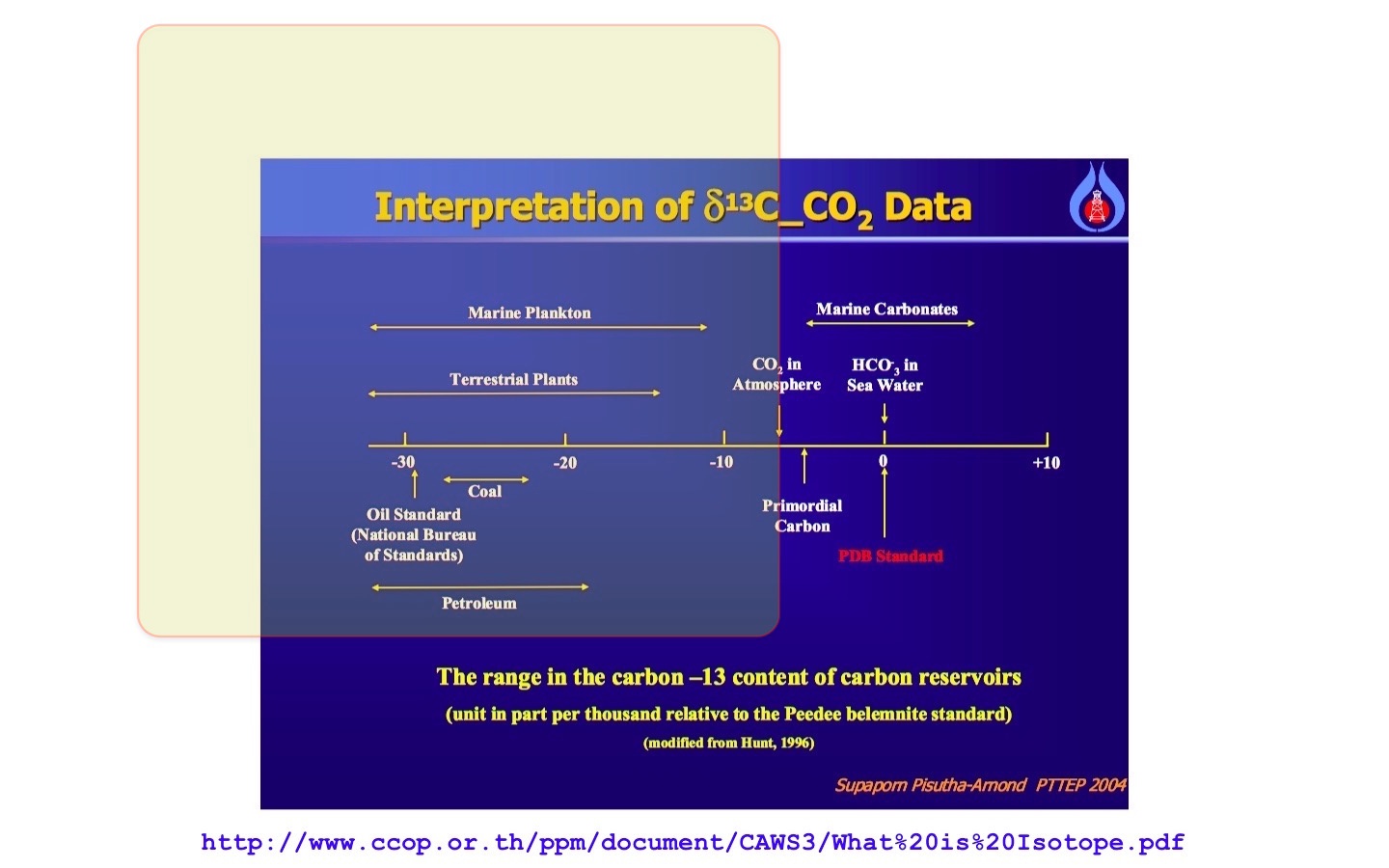 Terrestrial plants, and marine plankton are prime examples.
So, in the modern atmosphere, CO2 has a δ13C of about -8‰. Coal has a δ13C of about -23‰ to -28‰ Oil tends to be even further negative, -25‰ to maybe -33‰ …
But, there are many other sources that are even further in the negative region of δ13C. The isotopic shift mentioned by Keeling 2011 (above) simply means that a carbon source, with a more negative value of δ13C than the present CO2, is finding its way into the atmosphere.
So, any carbon source that vents to the atmosphere with a more negative value than about -9‰ would slew the present atmospheric δ13C to a more negative value … certainly, fossil fuel burning, will do that … but
Lee 2016 tells us: ”… biogenic δ13C values from soil CO2 studies along transform plate boundaries elsewhere, such as the San Andreas fault (−21.6 to −23.7 ; ref. 14).” The dilution of atmospheric CO2 with soil CO2 (as noted) will mimic Mannkind’s burning of fossil fuels.
Pisutha-Amond 2004 has a nice chart:
Jones & Grey 2011: ”An important characteristic of biogenic methane produced in sediments …, it is remarkably 13C-depleted (δ13C typically around -60 to -80‰; Whiticar, Faber & Schoell, 1986; Jedrysek, 2005; Conrad et al., 2007) compared with either allochthonous terrestrial plant detritus (δ13C value from C3 plants around -27‰; Peterson & Fry, 1987) or phytoplankton (δ13C typically around -25 to -35‰; Vuorio, Meili & Sarvala, 2006). Isotopic fractionation during utilisation of methane by MOB can lead to further 13C-depletion (by up to 20‰; Summons, Jahnke & Roksandic, 1994; Templeton et al., 2006).… strikingly low δ13C …”
Whiticar, Faber, & Schoell 1986: “Methane in marine sediments can be defined isotopically by δ13C −110 to −600‰, … In contrast, methane from freshwater sediments ranges from δ13C −65 to −500‰. …”
The dilution of atmospheric CO2 with oxidized biogenic methane, as noted, will mimic Mannkind’s burning of fossil fuels.
Brian, how about stating your argument and conclusion before
providing a bunch of quotes and links? I have no
idea what you’re trying
to say.
Clyde: the data
go way back.
Earth is not a greenhouse, CO2 is not the problem. Let’s look at who started and propagates this myth…
The UN & opportunistic, sympathetic governments like the USA who hope to cash in with taxes, fees and fascist policies to punish their population. The degree of covalent government involvement with globalist driven climate change in the USA makes me fighting mad!!!!
“The degree of covalent government involvement with globalist driven climate change in the USA makes me fighting mad!!!!”
Good! A *lot* of us feel the same way. We are in the process of straightening our government out on this issue. It’s taken a long time, but the tide seems to be turning.
And the temperatures are not climbing even with the extra CO2 in the atmosphere. Dishonest people may be able to manipulate the temperature charts to show warming, but they can’t manipulate a person’s personal thermometer. Reality will eventually set in.
This whole project by NASA using satellites and complex display graphics to identify sources, sinks and variations in CO2 was and is a colossal waste of tax payers money. Dig deeper into the science and discover that CO2 does not now, has never had and will never have a significant effect on climate.
Here is why:
1) Essentially all absorbed outgoing longwave radiation (OLR) energy is thermalized.
2) Thermalized energy carries no identity of the molecule that absorbed it.
3) Emission from a gas is quantized and depends on the energy of individual molecules.
4) This energy is determined probabilistically according to the Maxwell-Boltzmann distribution.
5) The Maxwell-Boltzmann distribution favors lower energy (longer wavelength) photons.
6) Water vapor exhibits many (170+) of these longer wavelength bands.
7) The Maxwell-Boltzmann energy distribution in atmospheric gas molecules effectively shifts the OLR energy absorbed by CO2 molecules to the lower energy absorb/emit bands of water vapor. The ‘notches’ in top-of-atmosphere measurements over temperate zones demonstrate the validity of this assessment.
8) As altitude increases (to about 10 km) the temperature declines, magnifying the effect.
@ Dan Pangburn
May 12, 2017 at 7:30 pm: Yes Dan, that is what real physics/icists know, along with the real role of water vapour, latent heat transport, the instantaneous expansion and buoyancy uplift from thermalisation. This will not go away, no matter what. Thanks.
That visualization clearly showed CO2 changes were seasonal, and then the narrator only asserted something assumed but not seen in the data, that is, mankind’s contributions to CO2 flux.
The CO2 flux in that data viz is completely swamped by natural fluxes.
The text of that presser stated, “It [CO2] is also influenced by natural exchange with the land and ocean.”
They can’t admit the global CO2 flux is vastly dominated by natural exchange.
OCO-2 was designed to detect and measure anthropogenic CO2 sources, based on what is stated in the technical design statements on their own site. In fact the data analysis show that those anthropogenic sources are NOT visible above the natural CO2 background, no matter how the data are massaged or visualized. The OCO-2 analysis confirms what biogeochemical carbon cycle biologists have always known, that humans do not have a detectable influence in the global carbon cycle. CO2 never accumulates in the atmosphere, it is constantly being scrubbed out into the vast subsurface pools at the rate shown in the 1964 atomic bomb 14CO2 curve. Even if human CO2 flux is now 4 percent of natural CO2, then the amount of CO2 in the atmosphere today is 4 percent of 400 ppm or 16 ppm.
Human CO2 is rapidly mixed in the atmosphere, and rapidly mixed into the natural CO2 sinks. Most of the increase in CO2 since 1850 is due to the natural flux increases that began with the exit from the little ice age, from biotic and abiotic (ocean) factors.
No.
OCO (the original which failed to achieve orbit) and OCO-2 were never inteneded to to just measure A-CO2.
OCO-2 is 3 spectrophotometers. 2 measure CO2-adsorption of wavelengths of the reflected sunlight, and 1 spectrophotometer is measuring an O2 relevant adsorption wavelength for relative comparison of CO2 adsorption bands.
Thus the OCO-2 sensors only measure CO2. There is no ability to discriminate natural CO2 adsorption from anthropogenic CO2 adsorption. To believe differently from that is to think that the measured O-C-O molecule “padsorption reading is that the column molecules “know” how to differentially adsorb IR radiation depending on whether they were predominately from a coal molecule reacting with O2 or a decayed leaf carbon reacting with O2.
joelobryan,
You said, “OCO (the original which failed to achieve orbit) and OCO-2 were never inteneded to to just measure A-CO2.”
While it isn’t possible to separate Anthro-CO2 from natural in the maps , I believe the original hope was to be able to identify anomalously high CO2 levels in the vicinity of major coal burning power plants and urban areas with high per capita consumption of fossil fuels. Thus, they could say, “See, we told you that Man was responsible for the increase in CO2.” Unfortunately (for the alarmists), it isn’t evident that Anthropogenic sources dominate, even in the NH. Anthro-CO2 isn’t even obvious in the US during the Winter, when plants and bacteria are dormant but humans are using even more fossil fuels to heat their homes. In examining past-published OCO-2 maps, I could see an area in China that appeared to be anomalous. The Amazon Basin looked unusual, and was perhaps a result of land clearing and burning. There were some unusual ‘hot spots’ in Indonesia that were more difficult to attribute to a particular source, but it again was probably forest clearing. The bottom line, from my inspection, is that natural sources dominate the production and sequestration of CO2 with very few exceptions. Thus, one cannot unequivocally state that the excess CO2 is anthropogenic because the other processes would continue in the absence of Man, and if some other process besides ‘greenhouse gases” was responsible for increasing temperatures then there would be increased oceanic outgassing, and that would lead to increased vegetation which in turn would create more CO2 when it dies and decays.
The OCO was designed with the intention to have the ability to resolve “regional” surface sources of CO2 from any source.
The underlying intention was to resolve anthropogenic sources from “natural” regional areal sources over a couple years with ground based calibration of the satellite spectrometers since the methodology of the satellites only worked from the boundry layer to about 10k altitude where the aircraft measured CO2.
I did not say, or intend to claim, that the OCO was designed to “only” measure anthropogenic CO2.
I’ve read some of the science mission statements and one of the underlying papers for the design of the OCO. My interpretation of the intent of the people who created the OCO was that they wanted to map the anthropogenic CO2 sources with the intention of confirming their pro-global warming political bias. It’s sad to see the obvious global warmist bias in NASA and JPL web pages for a “science” mission.
The current “analysis” and presentation of data also clearly show a warmist bias, they are trying to show something that is not in the data. It is obvious to anyone that looks at the graphics that anthropogenic sources of CO2 can NOT be resolved from natural sources. They underestimated the amount of smearing of 4 percent in the boundry layer. The OCO-2 could never look into the boundry layer in the first place.
BTW, I agree with Clyde’s response. The OCO-2 worked fine, it found exactly what most any biologist or biogeochemical cycle ecologist would expect for a global view of CO2 sources and sinks. If someone wants to fly the same spectrometers 1000 meters over a coal power plant, they could see the CO2 coming out of the smokestacks, but that’s not a global picture.
I’ve watched the clip a few times now including at YouTube’s 0.25 speed . I can’t see any indication that high concentrations are coming from the industrialized urban areas one AlGoreWarming blames . Indeed much seems to be billowing from biologically lush areas like equatorial Africa .
I will be getting to https://www.esrl.noaa.gov/gmd/annualconference/ in Boulder the 23rd & 24th . Their website is partially down for some maintenance this weekend , but I see from my notes from 2015 , I met David Crisp , one of the main guys in the OCO-2 project . I see he’s got a YouTube : href=” https://www.youtube.com/watch?v=JYyhMQzcVlY” > David Crisp: Measuring atmospheric CO2 from space – 24 April 2015 .
Struck me as a bright guy , one of the few who knows APL . I do hope he will be there again this year . Look forward to a much more extensive conversation .
Somehow I got that anchor syntax wrong . Worth highlighting the vid anyway .
Odd that it doesn’t have the world’s constant CO2 hot spot: Hawaii. Vulcanism. Every day.
I just watched the video. Maybe somebody already brought this up but, the title of the video says “seasonal changes” yet it only covers March 1, 2015 to July 31, 2015.
That’s about early spring to mid-summer. Hardly “seasonal” for either hemisphere.
So what happened when human emissions leveled off, as reported recently over, what is it, 2 years? No change in the Hawai’i measurements? No, it cannot be that they got it wrong. Perhaps they are still celebrating the lifting of guilt. Please share with us, beloved warmistas. Not that any of their gas budgets are worth a Tinkers Curse, bur all the same, we would like to know…..
OCO2 was a riposte to JAXA, which made Nasa-GISS look silly. Did not work out too well, so currently all is smoke and mirrors (with credit to Rud).
Brett,
With constant CO2 emissions, CO2 still would go up in the atmosphere, but as the CO2 pressure goes up, the sinks (oceans and vegetation) will absorb more CO2, thus the increase rate will go down. That will end when emissions and sinks are equal, that is at around 500 ppmv for the current emissions.
Why is the angle in the video chosen so that one cannot see the Northern hemisphere, or the location of CO2 on the map, instead of choosing a vertical look?
“During Northern Hemisphere fall and winter, when trees and plants begin to lose their leaves and decay, carbon dioxide is released in the atmosphere, mixing with emissions from human sources. This, combined with fewer trees and plants removing carbon dioxide from the atmosphere, allows concentrations to climb all winter, reaching a peak by early spring. During Northern Hemisphere spring and summer months, plants absorb a substantial amount of carbon dioxide through photosynthesis, thus removing it from the atmosphere and change the color to blue (low carbon dioxide concentrations).” == From this it is clear that during high CO2 regime in the atmosphere the energy availability to convert in to temperature through greenhouse effect is practically very low; and during low CO2 regime in the atmosphere though the energy availability to convert in to temperature through greenhouse effect is high the temperature rise will be low with low CO2. This clearly demonstrate that the global warming is insignificant with CO2 raise from fossil fuel burning.
Dr. S. Jeevananda Reddy
Previous animated maps from OCO-2 have shown that bacterial oxidation essentially shuts down during the cold Winter, except maybe in the southern US and in similar latitudes in Europe and Asia. When I have previously examined the OCO-2 maps I looked carefully to try to find elevated CO2 from places like the Four Corners power plants and urban areas heating buildings. I didn’t see it. It makes me wonder why it is now being claimed to be there.
They use the time honored technique of “Hand-wavium” to find anthropogenic CO2 source signals in OCO-2 data.
Same here, the basic data is being “massaged” to show only what they want to see. Read some of the statements of the mission scientists that created the OCO missions, clearly biased. The null hypothesis prevails, there is no significant anthropogenic source of CO2 in the global biogeochemical carbon cycle.
It looks to me that the “natural” sources and sinks were grossly underestimated. Certainly in the tropics.
bw,
Yes, I suspect that the researchers were surprised at the amount of outgassing from the tropical oceans and the rapid pull-down of biogenic CO2 by trees leafing out in mid-latitudes. But, that was the whole point of the OCO missions — to learn more about the carbon cycle. Now, if they would only learn from their experience and not try to put a spin on the data!
Dr. Reddy,
Average CO2 release by humans is 0.01 ppmv/day. Even if concentrated in about 10% of the earth’s surface and the ability of the satellite to focus on specific spots during a longer period, it will be a hell of a job to find the extra CO2 from human emissions.
Still there are other problems with the data, as in previous published monthly data, high levels of CO2 where found over the N.E. Atlantic, where on of the largest CO2 sinks is situated…
Actually, it’s about 16 ppm per day, or year, or at any time since the continuous flux rate reached 4 percent of the total CO2 flux. In the early 20th century anthropogenic CO2 flux was about 1 percent of the total. After several decades, the atmosphere reached approximate equilibrium at about 1 percent total CO2.
As the anthropogenic flux gradually increased to 2 percent of the total flux, the total CO2 mass in the atmosphere approached .02 times say 300 ppm, or 6 ppm of the total. By 1958 the flux was maybe 3 percent of the total, or was .03 times 315 which is nearly 10 ppm. Now that the third world is cranking out coal fired power plants, the amount in the atmosphere will approach 16 ppm, at the atmosphere equilibrates. Just as a river will equilibrate at a new level when you add 4 percent to the flow rate.
bw,
You are mixing a lot of things together which don’t make any sense…
Human emissions reach about 9 GtC/year nowadays or ~4.5 ppmv/year or 0.0123 ppmv/day worldwide.
Even if concentrated in 10% of the world’s total area, that still is only some 0.1 ppmv/day. Or about the resolution of the OCO-2 satellite.
The satellite only measures midst of the day, thus depending of (lack of) wind speed the 0.1 ppmv/day still may hang around or blown away into the bulk of the atmosphere. Even if they use the possibility to focus on specific spots to enhance the resolution, it will not be easy to trace the human contribution.
For the rest, the satellite can’t make a distiction between the origins of the CO2 it measures, it only measures concentrations. Thus no matter if the residual human CO2 in the atmosphere is 1% or 50%, the satellite can’t tell you what the real percentage is.
The measured drop in δ13C can tell you that: currently about 9% of the CO2 in the atmosphere is from the burning of fossil fuels, that is about 1/3 of all what was burned since 1850, the other 2/3 is distributed into other reservoirs, mainly the (deep) oceans.
CO2 (400ppm) is not “the most important” greenhouse gas, water vapor is (30,000ppm).
Since the end of the Little Ice Age in 1850, CO2 has contributed around 0.3C of global warming recovery out of a total of 0.83C, and because CO2 forcing is logarithmic, we’ll enjoy another 0.3C of warming recovery over the next 83 years…
The absurd CAGW hypothesis assumes around 0.4C of warming to date (close to actual), but goes off the rails by projecting 2.6C~4.1C of catastrophic CO2 warming over the next 83 years (0.3C~0.5C/decade trend), starting from….tomorrow—meh, not so much…
We should be ecstatic CO2 levels are returning to healthier levels, as we”ve enjoyed a 38% increase in global greening just since 1980 from manmade CO2 emissions (Zhu et al 2016).
Far from being scary, this NASA video shows how incredibly essential CO2 is to all life in earth…
P.S. Did the Russians hack Climate Change, too?
Water vapor is so variable that there is no point in expressing any average water vapor concentration.
It can be 40000 ppm over the tropical ocean surface, and drop to 400 ppm at the same place at higher altitude. One value that can be calculated from the global mass of water vapor in the atmosphere is around 2500 ppm. That number is sometimes used in some model calculations as an estimated starting point. I read a paper recently that found that water vapor never drops below 8 ppm in the high stratosphere.
Note that Astronomers are pretty good at putting their telescopes at high altitudes to get above the atmosphere not because of Nitrogen, Oxygen, and smog but because water vapor declines rapidly with altitude.
You’re correct that water vapor concentrations vary greatly over ocean latitudes and land mass areas. The 30,000ppm number is a rough global estimated average.
The salient point is that based on NASA’s NVAP (water vapor project) satellite data, there hasn’t been an increasing global trend of water vapor since 1990, which invaldiates CAGW’s crucial assumption of a rapid runaway water vapor feedback loop that’ll cause the 3.0~4.5C of catastrophic CO2 induced warming by 2100…
CAGW is dead.
@ SAMURAI
May 12, 2017 at 9:15 pm: The Russians are not stupid; they do not believe in CAGW (having perhaps seen marxist lies before).
They do however have the best model, which uses solar and oceanic factors, IIRC.
Brett-San
I was being sarcastic about Leftists blaming everything on the Russians these days…
“The Russians are not stupid”
A competitor is not going to interrupt their adversary when he’s doing something stupid, though.
Its true C02 is a trace gas. It cannot warm the planet or make it greener
Water and sun explains everything
Mosher-san:
CO2 levels below 150ppm is an earth-wide extinction event as photosynthesis shuts down.
Just since 1980, manmade CO2 emissions have increased global greening by 38% from the benefits of the CO2 fertilization process…
http://www.nature.com/nclimate/journal/v6/n8/full/nclimate3004.html
I’d like to know how the model generates a high altitude CO2 ‘sink’ when all the lower and surrounding regions are apparently higher in CO2 (the blue region above the North polar regions in the video). It isn’t being lost to space so how is it being reduced? Rained out? That would seem unlikely at an altitude of more than 15km. Something seems amiss.
Brewer-Dobson circulation? High-altitude air originates in upwelling at the equator perhaps providing an end-run for low CO2 air.
I posted the algorithm.
Go improve it.
you know … do science.
“I posted the algorithm.”
The AlGoreithm that you use to Mannipulate the data to match the
computer gamesclimate models, you mean?The final statement in the video is not supported by a few months of OCO-2 data. The overwhelming bulk of scientific data shows that changes in atmospheric CO2 are NOT caused by human factors. The OCO-2 video does show one fact clearly, that human sources of CO2 were not detected by a satellite that was specifically designed to detect anthropogenic CO2 sources.
CO2 never accumulates in Earth’s atmosphere from any source, any more than water accumulates in a river.
bw,
80 ppmv increase since 1958 is not an accumulation?
Of course not. Atmospheric CO2 that existed in the atmosphere in 1958 has entered deep sinks and will never return to the atmosphere. Some mixes into ocean deep water, some by biological pump raining onto the ocean floor and remaining as sediment. On a geological time scale the sediment eventually mixes with the deep geological carbon pool and will never return. A small amount of the deep ocean portion will start to return to the upper layer on a time scale of thousands of years.
One half of all atmospheric CO2 is removed in 10 years into those sinks that realistically never return to the atmosphere.
In 2007 the atmosphere CO2 mass was about 3000 gigatonnes. Only 1500 of those gigatonnes remain in the atmosphere 10 years later.
In 1958 there were about 2440 gigatonnes of CO2 in Earth’s atmosphere, only about 1/64 of that remains today, about 38 gigatonnes.
In one year, about 5 percent of all atmospheric CO2 is lost into the deep sinks. 50 percent in 10 years.
The 14CO2 bomb curve is obvious fact.
Of the 100 ppm increase from 300 to 400 ppm by volume, 20 ppm is anthropogenic, 80 ppm is due to a slight unbalance in long term ocean mixing and ocean surface heating since the little ice age. Atmospheric CO2 due to humans can never exceed the approx 4 percent annual flux rate, so about 16 ppm due to fossil fuel burning, and 4 ppm due to land use changes, tropical forest burning, etc.
At some point in the early 20th century when human addition was 1 percent of total CO2 flux, the percentage of CO2 in the atmosphere was about 1 percent of the total CO2 mass. 300 ppm by volume is 44/29 by mass, so about 0.00045 times the 2317 gigatonnes of total mass, which is 1 gigatonne.
When you add 1 percent to the flow of a river, the amount of water in the river can never increase by more than 1 percent. There is no accumulation at the point of entry, it all flows away into the far away ocean.
There is always water in the river, but it never accumulates.
bw,
Sorry, but you are mixing residence time (~5 years), which only moves CO2 between the different reservoirs, with the time needed to remove any extra CO2 injection in the atmosphere which has an e-fold decay rate of ~51 years. The latter is what removes CO2 as mass, the first doesn’t remove any CO2 mass after a full cycle, it only exchanges CO2 from one reservoir with CO2 from another one. That changes the isotopic ratios, not the total mass…
The 14C bomb spike is a mix of both, as what goes into the deep is the current level (which peaked in 1960), but what returns is the level of ~1000 years ago. That makes that the decay rate of the 14C bomb spike is at least 3 times faster than for a bulk CO2 spike, of which ~99% is 12CO2.
In 1960, some 97% of all 12CO2 sinks returned from the deep oceans, but only some 40% of 14CO2…
You can’t understand the obvious fact that 14CO2 represents natural CO2 exactly. They are chemically identical. There is no significant isotope effect. Your claim of tau at 51 years is rejected by the observed fact that tau is 18 years.
The entire branch of science called radiocarbon dating is based on the same observed facts. You will never find anyone to corroborate your claims. Bart is right in that your analysis is a circular confirmation of your assumption that all natural sources and sinks are balanced. Which is derived from the original assumptions for early biogeochemical carbon cycle balances.
The oceans (and biosphere and cryosphere) are equilibrating at a century scale response to the post little ice age recovery of global climate. Anthropogenic CO2 sources are not significant, and there are no net positive feedbacks on a global scale. Recent arctic melting is due to surface soot from asian coal plants.
It’s not a personal matter for me, you are just clinging to a convoluted interpretation that is not supported by the observations. CO2 can NOT accumulate in the atmosphere any more than water can accumulate in a river.
Try a fresh analysis of the global carbon cycle from the perspective of atmospheric evolution over geological time scales when the global mass of CO2 shifted into various geological pools, then when biology took over. The atmosphere is (currently) of biological origin, and has been for several hundred million years, that is why most physics types can’t understand what is going on. Global biological activity controls the amount of CO2 (and methane, etc) in the atmosphere. With some parallel obfuscation by the abiotic ocean that buffers the total biogeochemical carbon cycle.
bw,
You can’t understand the obvious fact that 14CO2 represents natural CO2 exactly. They are chemically identical. There is no significant isotope effect. Your claim of tau at 51 years is rejected by the observed fact that tau is 18 years.
Not only do I understand that fact, but I know that the decay of any excess 14CO2 above “background” is biased faster than for 12CO2, because less 14CO2 returns from the deep oceans than 12CO2, while at the sink side there is little isotopic change:
http://www.ferdinand-engelbeen.be/klimaat/klim_img/14co2_distri_1960.jpg
That means that in 1960 some 97.5% in mass of the bulk CO2 returned from the deep oceans in the same year as the sinks, but only 43% of 14CO2. That makes that the decay rate of any excess 14CO2 is much faster than for any excess 12CO2. Thus both a tau of 18 years for 14CO2 and 51 years for the bulk (12)CO2 are right.
data and simulations so as simulations can’t be perfect ( an data without uncertainties as well ) you know that you are looking to something somehow wrong…
Yes You see the same thing is the satellite “data” that shows a greener world.
All THAT satellite data is ALSO the result of models
Mosher,
You said, “Yes You see the same thing is the satellite “data” that shows a greener world.
All THAT satellite data is ALSO the result of models.”
I hope that they aren’t using unvalidated models to determine vegetation cover. It was my impression that the ‘greening’ event was determined using multispectral classification, or at least determining the Normalized-Difference Vegetation Index. No “modeling” necessary other than a conceptual one.
I saw the recent study showing ~ 9% greater forest than previously estimated was based on 1 meter resolution vs previously ~ 10m so it would seem their “modeling” is on the level of actual tree counting .
“All THAT satellite data is ALSO the result of models”
There are all sorts of models, Mosher, plastic models of aeroplanes, the equations I and others developed around half a century ago to optimise distillation column bubble caps, the models we developed in the 1970s to utilise noise cancellation effects to quieten cars without using heavy sound deadening material, the models that Boeing use when designing aeroplanes.
Then there are the “models” you dodgy “climate science” lot use, totally unverifiable, to model non-linear dynamic feedback driven systems subject to inter alia extreme sensitivity to initial conditions, bifurcation and heaven knows what other chaotic effects, when you don’t even come close to knowing the feedbacks and don’t even know the signs of some of the ones you DO know.
So take your model schtick and stuff it where the sun don’t shine, you’re not the only one to have programmed models – although I doubt you actually did at all, otherwise you would understand their limitations and wouldn’t have your quasi-religious faith in them.
“I hope that they aren’t using unvalidated models to determine vegetation cover. It was my impression that the ‘greening’ event was determined using multispectral classification, or at least determining the Normalized-Difference Vegetation Index. No “modeling” necessary other than a conceptual one.”
Wrong. You didnt read the ATBD
see the accuracy figures… R^2 .61
https://www.ncdc.noaa.gov/sites/default/files/cdr-documentation/CDRP_ATBD_056401B-20c.pdf
Primary Sensor Data are Bidirectional reflectance distribution function (BRDF)
adjusted surface reflectance data derived from AVH09C1 products. Sun zenith angle is also
used from the same products to retrieve the surface reflectance non-adjusted from the sun
geometry.
The map was produced by Hansen et al. (1998) for the period 1981-
1994. To avoid none consistent land cover changing, the same classification is used for the
entire data set. Moreover, to reduce the number of Artificial Neuron Network (ANN) and
spatial discontinuity, the number of classes were reduced from 9 to 6 (see Table 3)
The VJB model (Vermote et al. 2009) is used to retrieve nadir-adjusted surface reflectance
from BRDF- adjusted surface reflectance. The surface reflectance of the AVH09C1 product
are adjusted for the sun-view geometry to a constant view zenith angle (ϴv=0°) and a
constant sun zenith angle (ϴs=45°). However, the FAPAR is a variable that varies according
to the zenith angle. It is consequently more appropriate to derive FAPAR from nadiradjusted
surface reflectance keeping the original sun zenith angle through the
implementation of the VJB, for which the theoretical basis is described below.
The analysis of Parasol multidirectional data has shown that, among analytical BRDF
models, the Ross–Li–Maignan model provides the best fit to the measurements (Breon et al.
2012).
MODIS main algorithm is based on Look Up Tables (LUT) simulated from a threedimensional
radiative transfer model (Knyazikhin et al., 1998). Red and NIR
atmospherically corrected MODIS reflectance (Vermote et al., 1997) and the corresponding
illumination-view geometry are used as inputs of the LUT. The output is the mean LAI and
FAPAR values computed over the set of acceptable LUT elements for which simulated and
MODIS surface reflectances agree within specified level of (model and measurement)
uncertainties. When the main algorithm fails, a backup algorithm based on NDVI
(Normalized Difference Vegetation Index) relationships, calibrated over the same radiative
transfer model simulations is used (Yang et al., 2006). We retained pixel flag as derived
from the main algorithm and back-up algorithm.
FAPAR product corresponds to the instantaneous value at the time of the satellite overpass.
LAI and FAPAR are first produced daily. Then, the 8 days composite corresponds to the
values of the product when the maximum FAPAR value within the eight days period is
observed. Note that no LAI and FAPAR values are retrieved over bare or very sparsely
vegetated area, permanent ice or snow area, permanent wetland, urban area, or water
bodies.
but doesn’t that mean that Hansen’s “model” for vegetation has NOT been changed since 1994, when CO2 levels were significantly less that today, thus creating an error in interpreting how dark the planet is?
(More CO2 => more vegetation in ALL regions and ALL climates at ALL times of the year => a darker albedo => greater warmth because more solar energy is absorbed, more CO2 is turned into dark leaves and grasses in more areas and not reflected.
“So take your model schtick and stuff it where the sun don’t shine, you’re not the only one to have programmed models – although I doubt you actually did at all, otherwise you would understand their limitations and wouldn’t have your quasi-religious faith in them.”
faith in Models?
Never.
All models are wrong. some are useful.
Climate models are useful even if they are biased high
You talk about verifying models.
err NO
You test the skill of the model.
So when I built models of ESA radars I had to start with the physics. Of course we couldnt model all the physics because we had to work in real time.. basically 60 hz, although some models were so complex we could only update at 1 second.
The radar was pretty easy, There were 3 plates or attenae. Each installed at a different angle on the aircraft.
Each with a different number of modules In an ESA you electrically scan ( as opposed to a mechanical or gimbled radar). That scanning reduces your power at off normal angles ( its roughly a cosign falloff in power/ gain) Once you have that ( its basically a 3D operation) you have a volume that represents the power for the radar. Then you have to account for transmission losses, basic radar theory, and then you to account for the target RCS. You might be running different modes in your radar and each of those will have different parameters. The target might be doing ECM ( electronic counter measures ) so you have to account for those, Typicaly by raising the noise floor, unless you are doing a more exotic simulaton. Then you have to simulate whether the radar gets a return that it can detect .. and you have threshhold to work with. If you have sensor fusion you ight have data ( Line of Site ) from a passive reciever. At some point you declare a track and establish a target filter.
The target filters are typically kalmen filters where the physics of the filter correspond to typical figures for a jet aircraft. Once youve established track, then you start a process of deciding whether the track is good enoough to launch. This depends on the missile you are using and its sensor and sensor field of view. The missile will launch and fly a proportional navigation flight path using updates from ownship. However, at some point it turns on and you want to make sure it can see the target when it turns on and goes active.
Missile guidance and end game is also fun. It all gets even more complicated in the IR world where the sensor is vulnerable to countermeasures like, UV lights, Flares and end game maneuvers.
This was my bible, first edition was 1985
https://www.amazon.com/Fundamentals-Aircraft-Survivability-Analysis-Education/dp/1563475820
the basics are here ( mine is 1983 version), but that was just the start.
http://www.barnesandnoble.com/w/stimsons-introduction-to-airborne-radar-hugh-d-griffiths/1124315742?ean=9781613530221&pcta=n&st=PLA&sid=BNB_DRS_Core+Shopping+Textbooks_00000000&2sid=Google_&sourceId=PLGoP120&k_clickid=3×120
“You test the skill of the model.”
Which – in the case of your
computer gamesclimate models is approximately equal to zero, of course.Thing is Mosher, we are dealing with two very different types of model here. In the case of your radar and my bubble caps, after we’d constructed the models, we were able to test them for real, determine the limitations, omissions and errors in the models, adjust them to match the real world results, and continue in the loop until the models were so well optimised that they were of real value to design the equipment, what I would refer to as closed-loop modelling.
In the case of climate models, this is clearly impossible, we know far too little of the physics involved, and in any case non-linear systems are effectively computationally intractable, sensitivity to initial conditions alone ensures that – especially when claiming that the results can have value for making policy decisions affecting our policies tens – hundreds even – years into the future, so they are of no more than academic value, the fact that anyone is prepared to stake even the price of a can of beer – never mind $billions – $trillions even – on their prognostications is, as will become apparent in the not too distant future, perhaps the greatest and costliest policy mistake in human history, certainly comparable to the human and financial cost of the two World Wars.
Mosher,
What you are calling a “model” is referred to as a retrieval algorithm in the document you provided the link for. They acknowledge that the approach used has problems with the forest classes, especially trees with needles. One of the reasons is probably related to the coarse spatial resolution and limited spectral resolution of the sensors they are relying on. They went to a lot of work for problematic results, considering that Landsat data has been available for a longer period of time and has higher spatial and spectral resolution. The fact that a lot more trees have recently been found speaks to the deficiency of the approach of what you call are calling a “model.”
Am I reading this correctly that red is where taxpayer-funded “climate science” is the highest?
How can a sawtooth annual pattern created in the northern hemisphere survive its well-mixed encounters then show up at the South Pole? Geoff.
What’s with that colour range I don’t get it.
So … according to the animation, CO2 plummets to its lowest levels during the period of maximum ice melt in arctic. What does that say about the influence of CO2 on arctic ice melt?
Their logic is all of the extra CO2 induced heat ends up in the Arctic and Antarctic and deep oceans, pretty much anywhere there are no temperature measuring stations 😀
The comment regarding the stratosphere is not at all clear. What should a one year residence time have to do with being immune to CO2 emissions?
Looking at the CO2 in the video, the average globally would not be 400ppm but lower.
The video narrator uses false logic. Because we know the earth is greening, the amount of CO2 released through decay will increase along with the extra greening. Thrown in differences in how different plants adapt to rising and all other influences on plant life in the NH, like land management, in total huge tracts of land change year on year, mainly in the direction of clearing greenery.. draining wetlands ect.. and add our emissions on top of that.. how much do we really effect the long term trend?
A warming greening world is going to see CO2 increase year on year. CO2 producing lifeforms explode exponentially in warming climates, things like Termites. Sadly, this abstract method of deducing natural CO2 emissions are utterly flawed due to the fact that not only plants advance and retreat in summer n winter but so do a vast number of CO2 producing organisms which increase in population in warming climates.
Half baked science makes half baked claims, the CO2 origin question has one eyed biased assumptions, it’s hardly scientific to claim to know what amounts of Co2 come from where, given we don’t even measure human emissions let alone natural!!!!!!!!!!!!!!!!!
How much CO2 per year does all animals and humans combined exhale in total? 😀
Average human metabolism is about 1 kilogram of CO2 per day or .001 tonnes. For every 12 grams of carbon you eat, about 44 grams of CO2 is released. So you are eating about 270 grams of carbon per day.
So, 7E9 people release 7E6 tonnes of CO2 per day, which is .007 gigatonnes. 365 times .007 is 2.55 gigatonnes annual CO2 added to the atmosphere, which has a mass of about 3090 gigatonnes of CO2.
http://globecarboncycle.unh.edu/CarbonPoolsFluxes.shtml
The page uses atmospheric carbon value of 750 gigatonnes, which is an old number. Current atmospheric CO2 is 3090 gigatonnes, or 12/44 times 3090 tonnes for “carbon”, about 842.
Mark and bw,
What bacteria, fungi, insects and animals destroy or digest is converted into CO2, but that is CO2 which was captured by plants some months to decades before out of the same atmosphere. That is part of the biological carbon cycle, which is currently more sink (~1 GtC/year) than source. The latter is based on the oxygen balance, which shows that the biosphere as a whole produces more oxygen than it uses, thus more CO2 is absorbed than released by the biosphere… See:
http://www.bowdoin.edu/~mbattle/papers_posters_and_talks/BenderGBC2005.pdf
While interesting to know, it is not important in the total biological cycle, as not more recent carbon derivatives can be converted back to CO2 than were captured first by plants. At least not over long periods…
The main exception being fossil fuels, the result of millions of years of accumulation that we are bringing back into the atmosphere to the joy of most plants on earth…
Cheers bw, I had no idea.
According to a good piece written on here, the oil comes from algae that does not have a chance to fossilize. So fossil fuel it’s not 😀
Ferdinand, you have cited Bender 2005 before and I’ve read it before. Note the last sentence in the abstract. “…these fluxes are not understood.”
As a methods paper it deserves respect but they extrapolate a few measurements into a global assumption that happens to support the canonical Keeling hypothesis.
I can also cite a more recent peer reviewed paper that finds that the global oceans are a net source of atmospheric CO2.
http://reef01.marine.usf.edu/sites/default/files/project/cariaco/publications/Astor_et_al_2013.pdf
You can let me know why it is wrong after your read it. I can also cite papers that explain why the biological CO2 gradients in the uppermost ocean layer are underestimated. That means the biological component of biogeochemical fluxes of the oceans are actually underestimated. That means the actual guesses about the biological pump is underestimated and the upwelling CO2 is underestimated. Geological ocean bottom sources are underestimated, and CHANGES in global natural CO2 fluxes over century time scales are completely unknown. This is confirmed by the direct view of global CO2 fluxes by the OCO-2.
Since the anthropogenic CO2 estimates are known to be about 4 percent of global CO2 fluxes, at most, it is obvious that the remaining unknown addition of CO2 to the atmosphere is plausibly explained by the global ocean due to the recovery from the little ice age. It can’t be proved, but the simplest explanation is that the change in atmospheric CO2 is about 4/5 natural and about 1/5 anthropogenic.
bw,
If you cite someone’s work. please quote it literally with the relevant background.
“…these fluxes are not understood.” where the authors have measured these fluxes, which give the year by year variability, not the trend and they don’t know the origin of that variability…
The work of Bender looks at global changes in the oxygen balance, which shows that the earth is greening, the work of Feely e.a. looks at global ocean-atmosphere CO2 changes, which shows that the oceans are net sinks.
What you refer to is the measurements of one bassin just above the equator, which of course shows CO2 emissions. That is not global and can’t be extrapolated to global.
The biological pump is in fact included in the oxygen balance, as all plants, including sea plants, produce oxygen when performing photosynthesis. Once the oceans are saturated, any excess O2 production will reach the atmosphere and counted for…
CHANGES in global natural CO2 fluxes over century time scales are completely unknown.
Indeed, but so what? The net result is known: 800,000 years of a nice correlation between temperature (proxy) and CO2 levels mid the range of Henry’s law are more than enough proof that natural CO2 levels simply follow the temperature of the ocean surface. 290 ppmv for the current average ocean surface temperature. Not 400 ppmv.
Since the anthropogenic CO2 estimates are known to be about 4 percent of global CO2 fluxes
False reasoning from Bart, repeated by you: human emissions are up to 50% of maximum natural increase in the atmosphere over the seasons, not 4%. That is because ocean and vegetation fluxes are opposite to each other, largely cancelling each other out. Only human emissions are extra, each year again.
As only ~50% of all human emissions as mass is removed, the other half remains in the atmosphere and accumulates with the next half in the next year,…
“Carbon dioxide is the most important greenhouse gas released to the atmosphere through human activities.”
“Saliva via expectoration by baseball players is the most important fluid deposited on the playing field. We did not consider perspiration because it is not significant.”*
* We also did not consider precipitation. You know, like rain falling from the sky.
http://s1.postimg.org/ldp9fb6r3/climate_change_spitting.png
“Saliva via expectoration by baseball players is the most important fluid deposited on the playing field. … ”
One hopes .
Thank you Janice Moore for your kind words above.
For clarity, I do not necessarily suggest all or even most the observed increase in atmospheric CO2 is natural – like my friend Richard Courtney I am more of an agnostic on this subject. While this question is scientifically interesting, it is not critical to the assessment of the risks of catastrophic humanmade global warming (“CAGW”). One can make conclusions regarding the risks of CAGW with a high degree of confidence, without fully resolving the primary source of increasing atmospheric CO2.
It is incontrovertible that annual atmospheric CO2 flux (the Keeling curve) is dominated by natural seasonal temperatures – the cause of this seasonal flux is overwhelmingly natural and temperature-driven. It is also incontrovertible that atmospheric CO2 lags (in time) atmospheric temperature at all measured time scales (MacRae 2008, Humlum et al 2013 and others).
Since I wrote that conclusion in 2008, few climate scientists have wanted to even acknowledge this incontrovertible fact. To this day, the mainstream debate between climate skeptics and global warming activists continues to concern the sensitivity of climate to temperature (“ECS”) – or by how much the future can cause the past. 🙂
The following post attempted to focus the debate on what really matters – that based on the evidence, ECS is so small as to be insignificant, and the risks of CAGW are also similarly so.
Regards, Allan
https://wattsupwiththat.com/2017/04/12/perspective-needed-time-to-identify-variations-in-natural-climate-data-that-exceed-the-claimed-human-co2-warming-effect/comment-page-1/#comment-2477211
Excerpts from the following post:
All that really matters [in this analysis] is that CO2 lags temperature at ALL measured times scales and does not lead it, which is what I understand the modern data records indicate on the multi-decadal time scale and the ice core records indicate on a much longer time scale.
…
It also does not mean that increasing atmospheric CO2 has no impact on global temperature; rather it means that this impact is quite small.
…
What we see in the modern data record is the Net Effect = (ECO2S minus ECS). I suspect that we have enough information to make a rational estimate to bound these numbers, and ECS will be very low. My guess is that ECS is so small as to be practically insignificant.
Regards, Allan
Please excuse the pedantic nature of the following treatise – I am so often misquoted on this subject that I tried to make it very clear where I stand.
https://wattsupwiththat.com/2017/01/24/apocalypse-cancelled-sorry-no-ticket-refunds/comment-page-1/#comment-2406538
[excerpts]
I have stated since January 2008 that:
“Atmospheric CO2 lags temperature by ~9 months in the modern data record and also by ~~800 years in the ice core record, on a longer time scale.”
{In my shorthand, ~ means approximately and ~~ means very approximately, or ~squared).
It is possible that the causative mechanisms for this “TemperatureLead-CO2Lag” relationship are largely similar or largely different, although I suspect that both physical processes (ocean solution/exsolution) and biological processes (photosynthesis/decay and other biological processes) play a greater or lesser role at different time scales.
All that really matters is that CO2 lags temperature at ALL measured times scales and does not lead it, which is what I understand the modern data records indicate on the multi-decadal time scale and the ice core records indicate on a much longer time scale.
This does NOT mean that temperature is the only (or even the primary) driver of increasing atmospheric CO2. Other drivers of CO2 could include deforestation, fossil fuel combustion, etc. but that does not matter for this analysis, because the ONLY signal that is apparent in the data is the LAG of CO2 after temperature.
It also does not mean that increasing atmospheric CO2 has no impact on global temperature; rather it means that this impact is quite small.
I conclude that temperature, at ALL measured time scales, drives CO2 much more than CO2 drives temperature.
Precedence studies are commonly employed in other fields, including science, technology and economics.
Does climate sensitivity to increasing atmospheric CO2 (“ECS” and similar parameters) actually exist in reality, and if so, how can we estimate it? The problem as I see it is that precedence analyses prove that CO2 LAGS temperature at all measured time scales*. Therefore, the impact of CO2 changes on Earth temperature (ECS) is LESS THAN the impact of temperature change on CO2 (ECO2S).
What we see in the modern data record is the Net Effect = (ECO2S minus ECS). I suspect that we have enough information to make a rational estimate to bound these numbers, and ECS will be very low. My guess is that ECS is so small as to be practically insignificant.
Regards, Allan
*References:
1. MacRae, 2008
http://icecap.us/images/uploads/CO2vsTMacRae.pdf
Fig. 1
https://www.facebook.com/photo.php?fbid=1200189820058578&set=a.1012901982120697.1073741826.100002027142240&type=3&theater
Fig. 3
https://www.facebook.com/photo.php?fbid=1200190153391878&set=a.1012901982120697.1073741826.100002027142240&type=3&theater
2. http://www.woodfortrees.org/plot/esrl-co2/from:1979/mean:12/derivative/plot/uah5/from:1979/scale:0.22/offset:0.14
3. Humlum et al, January 2013
http://www.sciencedirect.com/science/article/pii/S0921818112001658
Allan,
CO2 lags temperature on all time scales (including current seasonal to 1-3 years) except for the period (1850-) 1958-current where CO2 leads temperature by 110 ppmv for the current average ocean surface temperature.
There is no ocean temperature on earth that can increase CO2 levels in the atmosphere beyond Henry’s law as seen in ice cores for over 800,000 years and over 3 million seawater samples in recent decades…
You are misapplying Henry’s Law. It only establishes the equilibrium point between oceans and atmosphere. It does not dictate the absolute level, only the ratio.
If the oceanic concentration increases, then the atmospheric concentration will increase in lock step, in accordance with the Law. And, a temperature rise throttles the transport of CO2 within the THC, which increases concentration within the surface layer of the ocean.
Ferdinand – you keep repeating this mantra and it is simply false.
CO2 lags temperature at all measured time scales – there are no proven exceptions.
Bart,
There is zero indication of any initial increase in the ocean’s CO2. The oceans follow the CO2 concentrations in the atmosphere, not reverse.
And a temperature rise at the sink area’s is good for 16 ppmv/K extra, while we are at 110 ppmv above steady state and locally 250 μatm more CO2 pressure in the atmosphere than in the ocean surface at the sink area’s.
And no temperature in this world can change the transport of CO2 within the THC or any other water (the “throttling” is only in your imagination), temperature only influences the exchanges between the ocean surface and the atmosphere in both directions, according to Henry’s law as above.
Allan,
From Etheridge e.a. CO2 at Law Dome ice core (~20 years resolution):
http://www.ferdinand-engelbeen.be/klimaat/klim_img/law_dome_1000yr.jpg
Temperature drop 1200-1600 ~0.8 K (Moberg, Esper,…); CO2 drop ~6 ppmv
Temperature increase 1600-2000 maximum as much as the drop 1200-1600; CO2 increase ~100 ppmv
Which is leading and lagging here?
You too Ferdinand – please read what I wrote!
Allan,
I have carefully read your texts since 2008 and commented several times…
Where my objections are is in the following sentence:
Atmospheric CO2 lags temperature by ~9 months in the modern data record
That statement is not right, what you see is: variability in the atmospheric rate of change of CO2 lags the variability in rate of change of temperature by ~9 months in the modern data record. Thus the noise around the CO2 increase lags the noise in temperature with ~9 months. That noise is not more than +/- 1.5 ppmv around a trend of +80 ppmv in recent decades and zeroes out in 1-3 years.
Looking at the noise in the derivatives can tell you that the noise in the CO2 rate of change is caused by temperature variability, but doesn’t tell you anything about the cause of the trend itself, as by taking the derivatives you have largely detrended the CO2 increase…
In this case, the CO2 trend leads the temperature trend beyond anything seen in the past 800,000 years and far beyond what Henry’s law says about the solubility of CO2 in seawater.
The Japanese, with GOSAT, deciphered the data in such a way that you could see the basic, large scale, CO2 sources and sinks. Inconveniently, they did not conform to the CO2 temperature control knob meme.
Later the initial OCO2 product did the very same. However, NASA has entirely obscured the basic, large scale, CO2 sources and sinks in their recent very elegant 3D visual.
How about it NASA…can we return to a much simpler, less elegant presentation of the data; one that reveals the basic, large scale, CO2 sources and sinks?
Sorry, bad for funding.
Why does NASA depict CO2 in orange and deep reds? Why not greens and deep blues? It is plant food after all. On the other hand, the roiling hot colors do lend excitement to the video. Reminds me of the “HELL IS REAL!!!” videos on YouTube; all the NASA mock-up needs to add is the wails of the damned.
go get the data. do your own color scheme.
Typically folks just pull a pre built color ramp or color theme from the package they are using
No.
I don’t think that video supports the notion of a thousand year residence time for CO2 in the atmosphere.
There’s another David Crisp video that’s well worth watching :
Note that Crisp spends only a sentence mentioning the issue of “climate” , but then gets quantitative .
This article by Erik Swenson back in 2015 gives the picture in detail.
https://wattsupwiththat.com/2015/10/04/finally-visualized-oco2-satellite-data-showing-global-carbon-dioxide-concentrations/
Compare the graphic for Apr 1 – May 15, 2015 with that for Jul 1 – Aug 15, 2015. Note that as soon as plant life in the northern hemisphere becomes active, the entire winter’s accumulation of CO2 is gone in 3 months. After reading this I am under no illusions about how long anthropogenic CO2 remains in the atmosphere.
Let’s be clear about OCO-2 it was launched to considerable fanfare and claims (largely borne out by some published results) that it had unprecedented accuracy and spatial resolution.
It would identify individual sources of CO2 as well as provide global coverage.
What have we seen ?
– in a single word obfuscation – driven in no small part by the instrument’s observations colliding with the prevailing hypothesis about how it all works.
So what would the earth be like without an atmosphere?
The average solar constant is 1,368 W/m^2 with an S-B BB temperature of 390 K or 17 C higher than the boiling point of water under sea level atmospheric pressure, which would no longer exist. The oceans would boil away removing the tons of pressure that keep the molten core in place. The molten core would rupture flooding the surface with dark magma changing both emissivity and albedo. With no atmosphere a steady rain of meteorites would pulverize the surface to dust same as the moon. The earth would be much like the moon with a similar albedo (0.12) and large swings in surface temperature from lit to dark sides. No clouds, no vegetation, no snow, no ice a completely different albedo, certainly not the current 30%. No molecules means no convection, conduction, latent energy and surface absorption/radiation would be anybody’s guess.
Whatever the conditions of the earth would be without an atmosphere, it is most certainly NOT 240 W/m^2 and 255K.
Model:
https://youtu.be/EGQsBmzFM_g
Reality:
If just falling leaves in SH autumn can overwhelm all the world’s cars, factories and power stations in CO2 emissions, even for only one month of the year, it puts anthro CO2 in perspective as of minor significance.
I find it amazing the NASA can turn the spot results from a satellite that orbits the earth completely every 16 days, into a data set that shows eddies etc of CO2 in 3D across the globe.
These eddies shown in the data to be fluctuating at a sub 24 hour timescale!!
Doesn’t the earth rotate as the satellite orbits, causing a 16 day lag before you get back to the same position above the earths surface?
Who knew they are this good!! /s
The Orbiting CO2 Observatory attempts to use a passive measurement of O2 opacity, and combines it with the active measurement of the tops of CO2 (ordinary air) columns, to arrive at a concentration ppv: http://www.atmos-meas-tech.net/10/59/2017/amt-10-59-2017.pdf
In other words, they are painting a picture by comparing apples with oranges