
Guest essay by Eric Worrall
h/t Janice – This video dates back to July, so it might not be news for some viewers. But the video elucidates in clear and simple terms why climate model error is actually far worse than those pretty spreads provided by the IPCC. I thoroughly recommend watching the video to anyone keen to understand why climate models are so bad at prediction.
YAY!!!!!!
Oh, Eric, THANK YOU, so much, for posting this — Christmas started early (well, ho, ho, ho, with Trump’s win, it started very late November 8!).
Excellent lecture, Dr. Frank!
Best wishes getting it unstuck from that monster of a peer review situation!
Janice
#(:))
Janice – you need to write for this web space – I have your 10 year compendium so I know you can …
I have two or three pieces already and have vowed (I have outlines but little time) for several more this winter. The Green Blob will NOT go quietly; we must be loud and constant.
Best,
Jim
Thank you, Jim. That was so kind and GENEROUS of you to say that. If I have anything I think worthy of the attention of this truly distinguished group (the WUWTers), I will do that. Thank you for your encouragement!
And you, with your 2 or 3, GO FOR IT! 🙂
Green Mob
I’d like to second Bubba Cow’s sentiments. I always smile when I see your name in the Comments, and I know I will appreciate what you have submitted. Janice, you are one of the regulars here that I can count on to help me connect this or that group of dots. I can honestly say this is one of the more interesting campaign seasons I’ve seen in my decades, and the issue of politicized science–and Mr. Trump’s recognition of its importance–has just made the headlines, for once in my memory for the better. Fastening my seat belt for a bumpy ride; I can’t wait to see the next budget discussions unfold.
Anyway, cheers, and have a very Happy Thanksgiving!
Oh, Mr. Newkirk. Thank you, so much. That really boosted my spirits today. HAPPY THANKSGIVING to you, too. Janice 🙂
Gang-Green guys! Gangrene!
And BRILLIANT, Janice. AGAIN. You are on a roll! 😀
Janice Moore,
What about the Cubbies? When the cubs won, I thought anything was possible.
Very happy about the Chicago Cubs’ win, too! (but, TRUMP trumped all, this year 🙂 )
Janice ==> Congrats, you have bullied Eric, at least, into posting the YouTube — which you had already included in yesterday’s comments.
I hope the moderator allows this here in reply, but — Thank-you Anthony for permitting my work here at WUWT. It does me honor.
Thank-you Eric for posting it, and Janice, thank-you Janice. Your support has been unflagging, good-hearted, and positive right from the start. Thank-you so much! 🙂
Thanks to everyone for your interest and comments. I’ll try to get to them all, but that’ll be mostly after work-hours. 🙂
Dr. Frank ==> It would be of great service to the readers here if your could supply a transcript of your lecture, with slides (which can be stills from the lecture video).
If a full transcript is not possible (I know I would not want to be asked to transcribe 42 minutes of lecture, even my own), maybe you can write out the main points as an essay with illustrations, or maybe you have a Powerpoint that accompanied your lecture, and you could combine that with commentary.
Most of the readers here are just that: readers rather than listeners or viewers.
I understand that you have had trouble getting papers published on this topic. If you have a paper you are willing to put into the public domain, it is quite possible that Dr. Judith Curry would post it — as a technical post – at Climate Etc. — which, frankly, is a more appropriate venue than WUWT for an in-depth technical discussion of the shortcoming of numeric climate models. Email me at my first name at the domain i4 decimal net and I’d be glad to send you Judith’s email address.
Moreover, if you are not a writer….not everyone is….I would be glad to whip whatever you can put down on [electronic] paper into a passable essay [which I have done for others in the past]. Same email address.
I will point out that you could have done this at any time in the past…Anthony has issued an open invitation to all for well crafted essays not only the topic of climate science, but “News and commentary on puzzling things in life, nature, science, weather, climate change, technology, and recent news “. (here)
You are so very welcome, Dr. Frank. Glad to do it. And I think Mr. Hansen is mistaken. Your lecture is exceptionally thorough, high-calibre, analysis. I doubt that anyone at WUWT needed to be “bullied” into publishing it. Reminded, yes. Forced, no. (as if I have the power…. wry smile) No, no forcings, lol, to post it just came naturally, I feel quite certain. 🙂
Hi Kip — thanks, you’ll find a presentation of the main findings of the model error analysis on WUWT here.
I also posted a discussion on WUWT of the truly incredible review comments I’ve received here.
The review comments post also discusses the problem that unique solutions are required for model expectation values to qualify as predictions. Climate models do not attain that standard.
Pat,
One thing that stuck out in the video was the remarkable improbability of the models aligning in the way they do, given the different inputs. I wonder though whether some viewers will appreciate the significance of this. It’s a bit like a dozen people leaving New York in different directions and randomly all turning up in Los Angeles exactly three days later. Either they had determined their destination in and arrival time in advance or there was some incredible subliminal force drawing them to that conclusion.
Nick, do you mean how the model cloud errors so strongly correlate? If I understand you, then you’re right. The correlated error clearly shows a problem common to them all.
“Nick, do you mean how the model cloud errors so strongly correlate? If I understand you, then you’re right”
But the whole basis of your cloud error calculation is the differences between the models.
That isn’t correlated.
Nick writes
You can clearly see each model does its own thing with clouds. There is is systemic error that they all share and that stems from the fact that clouds cant be modeled because we dont sufficiently understand them. I think it very likely that they all implement similar ad-hoc strategies to deal with them. Some have been tuned to be closer to “cloud reality” as far as overall coverage has been concerned, some so less so. The error, however, is shared.
I’m in agreement with your New York example, Nick. Though, my first mental image was of people from various New York City Environs, e.g. Bronx, Manhattan, Newark, Connecticut, Catskills, etc., leaving for their destination at the same time.
The chart of RMS errors appears to be misdirection.
In a 25 year retrodiction global average cloudiness calculation:
Is the RMS solely for the final calculated average or is it the sum of hourly, daily, weekly, monthly, annual averages of cloudiness?
Such a small standard error of deviation for global cloudiness averages over 25 years of calculations or measurements, appears rather disingenuous; for surely there must be days/weeks where the error is much higher, if not 100%.
A GCM 25 year run, that bases an error rate solely upon the final determination, implies we should all ignore 24.9 years of the GCM run.
As the actual GCM model runs demonstrate so well, errors summarize; even when calculated in quadrature, the result is a sum. Every module, every formula run has it’s possibility of error and error summation that should be carried forward to the end. An end is not after 25 years, but every determination point reached by the program during processing; rainfall, temperature points, humidity, cloudiness, winds, fronts, SST, etc.
Nick Stokes, “But the whole basis of your cloud error calculation is the differences between the models.”
No. The basis of the cloud error calculation is the difference between the simulated cloud cover and the observed cloud cover.
“The basis of the cloud error calculation is the difference between the simulated cloud cover and the observed cloud cover.”
The models are on both sides of the observed, so the errors clearly aren’t correlated. But in fact, it’s the model differences that you actually know. The uncertainty in observed is much greater.
Lauer and Hamilton Table 4:
That is 10% in CA (cover), which means the uncertainty on observed is as large as the total range of the CMIP5 numbers. And the SCF/LCF, which is the actual TOA flux, has an uncertainty on observation of 5-10 W/m2. That’s more than the discrepancy of 4 W/m2 you are quoting for GCM “error”. The errors you are attributing to GCM’s are less than the uncertainty of the observations you are comparing with.
Nick Stokes, “The models are on both sides of the observed, so the errors clearly aren’t correlated.”
Not correct. Model cloud errors are correlated. The 20th slide shows the error correlation matrix. Of 66 inter-model pairs, 58 show correlation R≥0.5.
You’re right about the uncertainties in the observations, Nick. I didn’t include them because I wanted a focus on model error alone.
Including observational uncertainty doesn’t help your case at all, though. We’re interested in the uncertainty in a projection. The total uncertainty entering into any given projection would be the simulation uncertainty relative to observations added in quadrature to the observational uncertainty against which the model calibration simulations are measured.
So, taking the average of your 5-10 W/m^2 uncertainty in observations as representative, the total uncertainty in the tropospheric thermal energy flux in every simulation would be sqrt(4^2 + 7.5^2) = ±8.5 W/m^2. That value should then be propagated through a projection.
The uncertainty bars expand accordingly. You’ve made the situation worse for yourself.
These are only cloud uncertainties, of course. Total energy flux errors of GCMs are easily an order of magnitude greater. A full accounting of uncertainty propagated through a projection would produce sky-high uncertainty bars.
Pat,
“The total uncertainty entering into any given projection would be the simulation uncertainty relative to observations added in quadrature to the observational uncertainty against which the model calibration simulations are measured.”
No, that is completely backward. The fact that a result is hard to observe does not detract from a model; it’s often the reason the model was used in the first place, eg in astrophysics or seismic modelling to locate oil. Models quantify what you can’t observe well. If you could, you would have less need of a model.
That is what is wrong with the logic you have here. The fact that cloud cover differs from observed means nothing, because the difference is less than the uncertainty of the observation. The fact that models differ among themselves is more significant, but just says that it’s one of the things models don’t do that very well. There is no reason why a model might not predict temperature well, as Hansen’s did, even with uncertainty about cloud cover. The thing is, you have created a toy model which makes it an input, which it isn’t in GCMs. And then you claim that the error propagates as in your toy model.
Nick, “No, that is completely backward.”
No, that’s exactly the way uncertainty is calculated. In the physical sciences, anyway. Physical magnitude uncertainty and modeled magnitude uncertainty combine in quadrature to give the total uncertainty in the model expectation value.
You wrote, “Models quantify what you can’t observe well. If you could, you would have less need of a model.”
First, in the physical sciences, physical models make explicit falsifiable predictions, regardless of whether the observable is obvious or not. Observables test the model. That well-verified models are used to make useful predictions is beside that point.
Second, strongly verified falsifiable physical models provide the meaning of observables; the why of why is oil found here and not there; of why stars of certain masses have certain temperatures; of why why n-butyl lithium is instantly pyrophoric in air. None of it is due to angels or demons. Physical theory provides the causal meaning.
You wrote, “The fact that cloud cover differs from observed means nothing, because the difference is less than the uncertainty of the observation.”
But the observation is what the models are trying to simulate, Nick. Their systematic difference from the observation puts an uncertainty in the model expectation value. The uncertainty in the observation puts an uncertainty in the model target.
The total uncertainty in the model expectation value is the combination of the two.
The simulation uncertainty is a property of the physically incomplete and uncertainly parameterized models. It would almost not matter what the target cloud cover was. The models would produce a similar simulation uncertainty.
This is demonstrated, for example, in the similar systematic model uncertainty produced in cloud cover when the target was the previously accepted value of 58% global average cloudiness. See the SI (892 kb pdf) of my Skeptic article for this example.
You wrote, “There is no reason why a model might not predict temperature well, as Hansen’s did, even with uncertainty about cloud cover.”
So you’re saying that despite not knowing the annual tropospheric thermal energy flux to within 2 orders of magnitude of the CO2 perturbation, the consequent air temperature change can be accurately modeled. Earth to Nick, over . . . . 🙂
Hansen’s model did not predict air temperature in any physically meaningful way.
You wrote, “The thing is, you have created a toy model which makes it an input, which it isn’t in GCMs.
It’s not a “toy model.” It’s a GCM air temperature emulator. And it’s demonstrated to do a great job. GCMs do indeed include cloud uncertainty as an input, Nick, whenever uncertain cloud parameters are inserted. What isn’t given is the output uncertainty following directly from the input uncertainty. Seriously negligent oversight, anyone? How competent is that?
You wrote, “And then you claim that the error propagates as in your toy model.”
No. I claim uncertainty propagates as the models simulate. And GCMs are demonstrated to simulate air temperature as a linear extrapolation of forcing. Linear propagation of error follows rigorously from that.
I’m an uneducated simpleton from the heartland.
I visit this site everyday
I am personally responsible for about 25 tons of steel and 100 gallons of high solids baking enamel paint, everyday. I pass out paychecks every Friday to the people that make that happen.
Our paint line runs at 60fpm, proud of what we do.
We get inspected twice a year, not by the lo.al guys, they come from Atlanta
thanks for your work – and vote
You caught the essence, Nashville. It’s all about professional competence and integrity.
Way to go Nashville. You are the real american engine!
If I recall correctly, his graphs had error bars +/- 15 C. That’s unreasonable because the planet has never seen temperature changes that big in the last five million years. link I think we are looking at a statistical exercise which is at least as far removed from physical reality as the models themselves.
I agree that the models are crap. I’m not sure this exercise actually proves that point.
Pat Frank is careful to distinguish the model error from what is physical possible – the +/- 15C is evidence the models are rubbish, not evidence that global warming could be +15C.
Bob, this is just saying that, given the methods used in the models, results of +15, -15 degrees and everything in between are equally as likely of being true, that is all we can infer from them. The nice colored lines in the middle are not the only results.
I thought the error bars usually indicate the 2 sigma spread.
Hi, Bob (c.),
Watch the video around 16:50 and you will see that Dr. Frank shows that average cloud error (of models) is + or – 140%.
Then, at around 26:40 on and you will see that Dr. Frank is discussing the GCM annual thermal cloudcover uncertainty (error) propagation.
Try watching the whole video — it really is worth the time!
Janice
That just about describes the whole fiasco. The feedback or in reality the damping is far higher than they need to make the the C in CAGW stick.
It proves mathematically that the models are useless. Period.
Not exactly, but .the models used by ipcc to predict temperature evolution,If you want to understand how climate works on a physical point of view, models are needed.
Models are not useless but you have to be very careful dealing with them, and at least test them the way this gentleman do. You shoudl even torture them a bit.
No, as process models (tools to study weather/climate) they could very well be quite useful. That’s what they were originally designed for. But for the purpose of telling us what the climate could be in the future, they are indeed rubbish.
commieBob
If I can help, the errors that are being discussed are not those that might actually occur in nature. They are just telling us if you used this model to describe the world how far you could end up away from where the world was really at. It tells you how good your model is as a predictor.
I should add that it relies on the assumption that the simple linear model would still fit the GCMs with different theoretical assumptions about cloud behaviour, and that the error paths are each equally likely. These both seem unlikely given what we know about actual climate behaviour, as you point out.
HAS, the emulation model error does not say all paths are equally likely. It takes the average CMIP5 error and calculates an average uncertainty. Average error is not the same as “equally likely paths,” and does not constitute an assumption. It is representative, as are the uncertainty bars.
The uncertainty bars don’t tell us how far the GCM simulations could end up from reality. Instead, they show that CMIP5 simulations have no predictive content.
Finally, the model emulates how GCMs treat forcing. How GCMS treat net forcing would not depend on how models calculate clouds. Different theoretical assumptions about cloud behavior would just change the cloud error modulus of the GCMs. The structure and magnitude of their cloud error might change. This could impact the magnitude of the long wave cloud forcing error.
That, in turn, would affect the size of the uncertainty bars as the error is propagated step-wise through a simulation. One doubts, however, that the uncertainty would be much smaller or that there’d be any significant improvement in the predictive content.
CommieBob, you comment illustrates one of the very points Dr. Frank was making, which is that there is a very poor understanding of the difference between precision and accuracy. After many thousands of runs of a climate model you will probably get a nice distribution of variances from the mean forecast, but all you have is a pile of rubbish shaped like a normal distribution. He was very clear that the climate will not produce actual temperatures in the +/- 15 C range.
commieBob, the ±13 C in the head slide is an uncertainty statistic, not a physical temperature. It marks a kind of ignorance width.
The large uncertainty just says that after 100 years of model simulation error the accumulated ignorance is so large that the future simulated climate has no knowable correspondence with the true future physical climate.
Eric Worrall’s reply captures this idea. So does oeman50’s, although I wouldn’t want to defend that all temperatures between ±13 C are equally likely. 🙂 Better to say that the models give us no idea what the future temperature will be.
Mark W, believe it or not, those ±13 C uncertainty bars are 1 sigma. 🙂 They are the result of systematic error, of course, which means they’re not strictly statistically valid. But they do give a good indication of the reliability of the projection.
Listen carefully to the last part again. He specifically says that those error bars do not represent physically realizable temperatures, they represent a range that the truth must be within – somewhere. The whole point is that the error bars are so huge that the projected temperatures are nonsense.
Right on, Paul Blase. 🙂
I would assert that the error bars are so huge (and so far from reality) that the modeling approach is useless and hence nonsense. They should toss the current “model” because it fails the definition of “model”.
Agreed, Rocky. 🙂 Doesn’t mean they shouldn’t try to improve them. But that would require getting back to the hard gritty work of experimentally-driven, detail-oriented, reductionist science. No more video gaming.
I don’t really know what to make of this.
Parts of it I understood:
The reduction of these immense piles of moldy Fortran to close approximation by a simple linear function of GHG levels was lovely.
Also, he convinced me that the various Global Climate Models (GCMs) share major systematic errors w/r/t the modeling of clouds (which is completely unsurprising).
He was also persuasive in pointing out the critical difference between model precision and predictive accuracy.
However, it looked to me like he added the imprecisions of ten GCMs in quadrature to reach the conclusion that the ensemble projection was far less precise than any of the individual GCMs. It appeared that he neglected to divide by ten!
Surely not? What am I missing?
Ask Pat. I missed that, I’ll have to rewatch.
I understand what you are saying, if all the models share the same systemic error it’s difficult to see why the ensemble would be worse than individual models.
Be fascinating to see Pat’s explanation.
Well, if their errors were entirely independent, combining ten of them would yield an large improvement in precision, because you’d be adding 1/10 of each of their error margins in quadrature. (E.g., if each of the ten had an error margin of ±1 the ensemble error margin would be ±sqrt(10×(1/10)) = ±0.316.)
But if the errors were entirely systematic then combining them would yield no improvement in precision at all. just the simple average of their error margins of all ten.
Reality is certainly somewhere between those two extremes. My guess is that they’re more systematic than independent, but that’s just a guess.
Pat stated quite clearly (at least I thought it was clear) that the model errors were systemic. That was the point of the intra- and cross-model correlations and the probabilities of 10^-17 and 10^-5.
If the climate is modelled as the chaotic system that it is, then that doesn’t have to be true whether we are talking about accuracy or precision. The best we can do is look for attractors.
Taking the average works for linear time-invariant (LTI) systems. Time-invariant means the system behaves the same today as it did yesterday. Here’s an example of where that doesn’t work:
If I average the tests I do on Wednesday, the result might look accurate and precise. If I repeat the tests on Saturday and include those results in the data set, my supposed accuracy and precision have gone out the window.
commieBob, a central point is that I’m investigating climate model behavior, not the climate itself.
The emulation model shows that climate models merely linearly extrapolate forcing, to get air temperature. There’s no evident chaos in their temperature output. Therefore, direct linear propagation of error directly follows.
daveburton,
It is my understanding that when the same observer takes multiple readings with the same instrument, on the same measured parameter, the increase in precision is proportional to the square root of the number of readings. Violate any of those assumptions, and the relationship fails. That is, taking the average of a large quantity of random numbers does not justify reporting a mean with more precision than the number with the least number of significant figures. Furthermore, in an ensemble, logically there can only be one “best” result. Taking an average of it along with all the poor results should result in a less accurate representation of reality. The precision of an inaccurate value is of little value.
Just a nit, but GCM is an initialism for general circulation model, not global climate model.
Thanks, Mark. Sometimes I amaze myself with my own flubs. I managed that one despite having GCM in my own web site’s climate glossary. Impressive, eh?
Hehe.
Mark T,
Even Judith Curry makes that mistake.
Thank you, Clyde. You’ve just made me feel a lot better! 🙂
But I just noticed another flub. I had a typo in my 2nd comment.
±sqrt(10×(1/10))
should be
±sqrt(10×(1/10)²)
Sorry about that.
He used the simple model and insert the error into it to give himself a measure of how the GCMs would have performed across the theoretical error range. It saves on re running the models adjusted for the theoretical error. It does however make some critical assumptions that I’ve noted above.
HAS, if by “theoretical error range” you mean a ‘perturbed physics’ study, or a ‘parameter sensitivity study, with variances relative to an ensemble mean, that’s not what the model shows. Those two sorts of studies only reveal model precision.
The uncertainty bars derived from cloud forcing error reflect the lack of predictive accuracy.
Dave ==> You see now one of the reasons that this “important” lecture, which was delivered to a conference of Doctors for Disaster Preparedness in July this year, did not make headlines in the climate skeptic blogosphere.
The blog meteoLCD did their homework and presented a essay with slides on it, and posted a corrected/revised version recently here.
The topic of the unreliability and uncertainty of climate models has been a major topic of discussion in the climate skeptic world, and recently covered several times, once by myself, at Judith Curry’s Climate Etc.
The “Climate Models Are NOT Simulating Earth’s Climate” series by Bob Tisdale and the Chaos and Climate series by myself, as well as more technical discussion of the details of climate models have taken place at Dr. Curry’s blog and here at WUWT.
In case you’ve missed it, it is common knowledge in the mathematics world that climate models, as well as fully acknowledged by the IPCC, that climate models cannot provided long-term prediction/projection of future climate states. They simply can not.
One more lecture on the subject (or even one more blog essay, for that matter, even mine) is hardly earthshaking.
Kip, my study is the first ever to propagate error through an air temperature simulation, and to provide physically valid uncertainty limits. Bob’s presentation is acute, but he presents no error bars. Neither did you, in your essay.
There are a number of reasons why the seminar might “not make headlines in the climate skeptic blogosphere,,” the simplest being that none of the principals knew of it. Other reasons might be less complimentary.
If it really is true that, “it is common knowledge in the mathematics world [and] fully acknowledged by the IPCC, that climate models cannot provided long-term prediction/projection of future climate states,” as you have it, then it must be that the IPCC is consciously lying about there being 95-100% probability that human GHG emissions are affecting the climate.
And that the IPCC has been playing that lying game ever since 1995, when Ben Santer injected his “discernible human influence” into the 1995 SAR. Is that what you’re implying?
We all know that the claim of a CO2 impact on climate relies 100% on the reliability of climate models. Mine is the first study to put a quantitative face on their unreliability.
It also puts the IPCC and its alarmist claims to bed as incompetent, and shows that every single air temperature modeling study since at least 1987 has been physically meaningless.
Is that “hardly earthshaking“?
Dr. Frank ==> Having read your two previous WUWT posts, and your comments here, I can see why you are having trouble getting your papers published and gaining an accepting audience with climate modelers.
Your approach seems to be that used by Sir Richard Francis Burton, English explorer of the 19th century — attack the living *bleep* out of anyone showing the slightest sign of opposition or disagreement. You don’t seem to be able even to get along with people who agree with you and offer their help. Note: This didn’t sit so well with his colleagues either.
You do seem to grasp the essence of the Climate Wars — both sides vehemently attacking the other, both blind to viewpoints of those who ought to be their colleagues — and when (unsurprisingly) these attacks don’t change the minds of their opponents, descend to name calling and denigration. You have already pointed out how well this has worked for you.
Good luck with your research and career.
Thanks, Kip. I’ll leave you to your opinion.
daveburton, the thermal cloud error is systematic, not random. Your second post picked up on that. The cloud error is heavily correlated across models, so it appears they’re making a common theory-bias error. That is, an error stemming from a mistake in the deployed theory common to all the tested models.
In the systematic error case, the step-wise errors across a given simulation combine into a root-sum-squared uncertainty.
The average of simulations then is subject to the root-mean-square of the uncertainties in the individual runs.
Randy Stubbings, you got it exactly right. 🙂
“In the systematic error case, the step-wise errors across a given simulation combine into a root-sum-squared uncertainty.”
There is so much bizarre wrong stuff here. Systematic errors just add, with sign. It is random errors, with cancellation, that accumulate with summed squares (variance).
We’re talking about the accumulated uncertainty, Nick, not accumulated error. Uncertainty accumulates as the rsse of each step in a simulation.
“We’re talking about the accumulated uncertainty, Nick, not accumulated error. “
Really bizarre. The statement says, again:
“In the systematic error case, the step-wise errors across a given simulation combine into a root-sum-squared uncertainty.”
So what measure of “uncertainty” makes it different? And what is the basis for sum-square accumulation?
Nick, the rss uncertainty follows from the fact that the projected temperatures are a linear sum.
The uncertainty is propagated using the CMIP5 average long wave cloud error statistic, ±4 W/m^2; entering it into the linear emulator as an uncertainty in the simulated tropospheric energy flux, of which CO2 forcing is a part.
” the rss uncertainty follows from the fact that the projected temperatures are a linear sum”
No. RSS would follow if the changes are random. Or possibly fluctuating in some other way with cancellation. But you say here:
“the thermal cloud error is systematic, not random.”
And that seems to be the theme of your talk.
The confusion is in your slide at 13:14. You do show the errors ε₂₀₀₁, ε₂₀₀₂ etc adding. But you say the year to year “uncertainty” adds via RSS. That makes no sense. If you have a systematic error in forcing, then yes, with your linear formula you can say that has maybe a 0.01°C effect in each year, additive. There is no associated “uncertainty” that adds differently. Even if you are uncertain about the 0.01, and maybe it should be 0.011, that doesn’t fluctuate year to year in a way that would justify RSS.
Nick writes
It does make sense. Ask yourself what it means in how the model works that there are demonstrable errors in clouds when compared to reality. And yet the model appears to behave…
Nick Stokes, “No. RSS would follow if the changes are random. Or possibly fluctuating in some other way with cancellation.”
RSS is how the uncertainty propagates through any sum, Nick. For z = a+b+c+…, then ±u_z = sqrt[(u_a)^2+(u_b)^2+ …], where “u” is ‘uncertainty in.’ GCM projected air temperatures are mere linear sums.
Nick, “The confusion is in your slide at 13:14. You do show the errors ε₂₀₀₁, ε₂₀₀₂ etc adding. But you say the year to year “uncertainty” adds via RSS. That makes no sense.”
It makes complete sense. Uncertainty is not error. Error adds with sign. Uncertainty adds as RSS. Uncertainty reflects the mistakes in the underlying physical model. Those mistakes in physics remain regardless of off-setting errors.
An answer of correct magnitude obtained because of off-setting errors tells you nothing about the physical system, and does not indicate that the physical model has predictive powers. Large uncertainty bars correctly informs that the result from off-setting errors has no physically meaningful content.
He looked at one (!) source of error not accounted for by the models and demonstrated that the error produced by this one source alone (the failure to properly model cloud cover) is far greater than any predicted “greenhouse effect”, to the point where the models are useless. He also pointed out that for all of their complexity, the models boil down to one simply linear function, meaning that they do not and cannot actually be modeling the complex non-linear behavior of the real world.
” He also pointed out that for all of their complexity, the models boil down to one simply linear function, meaning that they do not and cannot actually be modeling the complex non-linear behavior of the real world.”
Well, that’s completely wrong. What he might have reasonably claimed is that the ensemble average surface temperature of a group of models progresses linearly. It’s clear from the graphs shown that that is not true for individual model runs.
But the notion that that is all they do is just absurd. They deal with the whole atmosphere. Winds, water vapor, radiation, heat transport. It isn’t just surface air temperature. And the fact that one derived ensemble average means “they do not and cannot actually be modeling the complex non-linear behavior of the real world” is just silly. I’ll show again, just one example of a GCM modelling lots of complex non-linear stuff and getting it right:
Nick writes
No. That video shows weather, not climate. Climate change is due to the gradual accumulation of energy by the earth. That’s what the GCMs must resolve. The video you keep presenting as evidence of them getting complexity right simply shows a whole lot of weather and has nothing to do with climate.
GCM energy-flux errors show that the models do not partition the energy correctly through the climate sub-systems, Nick. The video you posted shows impressively complex numerical modeling, but does not indicate any of the uncertainty in the result.
One of the hazards of modern science is that computer graphics make intuitively compelling displays. Your video is a case in point. How can something so pretty be wrong? And yet, the known large-scale flux errors of GCMs tell us that it must be so.
I recall Carl Wunsch pointing out that the ocean models do not converge. I doubt this problem has been resolved since then, and recall asking you on Steve McIntyre’s CA what the meaning was of the results from a non-converged model. I don’t believe you ever answered. The question applies equally well to your video.
Excellent presentation, well organized and easy to follow.
It saddens me that the climate community is so corrupt and are unwilling to consider other scientific concepts such as this.
Thanks, keep trying, there may be a new Sheriff in town to straighten things out, it will be a challenge though.
Thanks, Catcracking. We’ll see what happens.
video at 17:30 f “The average error in all of these climate models is 12.1 percent error in cloudiness…. The total excess greenhouse gas forcing since 1900 is 2.8 watts per square meter which means that the error in the thermal content of the atmosphere is larger than the total forcing of all of the greenhouse gases since 1900.”
Amazing, isn’t it. Mike. Strange, too, how the IPCC and the climate modelers somehow neglected to pass along this bit of information, isn’t it. 🙂
Pat
I remember your post about the temperature uncertainty and the real systematic uncertainty being in the order of degrees. Something that should be blindingly obvious to any technical person that if you don’t design your measurement equipment to measure to a certain resolution with uncertainty don’t expect it to suddenly read at a better resolution than that. And that if you aren’t maintaining what resolution and accuracy you do have with regular characterisation and calibration, don’t expect even that to be met.
I’ve had discussions on Bishop Hill about the SST adjustments and it’s the same story. Uncertainties are treated theoretically rather than realistically. My take on this is the same: I don’t mind science papers about this but I do mind if this is used to drive policy. Because once it is in the realm of policy then it needs to conform to safe use as do all other performance data sets. Or it comes with a massive disclaimer which makes its use moot.
mickyhcorbett75, I completely agree with your take on the matter of instrumental resolution, and the need for professional integrity in its application to policy. A lower limit of accuracy in the land-surface air temperature record is about ±0.5 C; all due to systematic measurement error.
Like you, I’ve looked at SST as well, and have found a couple of calibration studies that show even Argo floats show temperature errors also of about ±0.5 C. Sometimes more. The lab-calibrated accuracy of Argo sensors is at least an order of magnitude better than that, indicating a source of systematic error in the field (ocean surface) measurements.
I’ve also contacted researchers about this problem. They’re resistant to it, and they’ve expressed confidence that the Central Limit Theorem plus the Law of Large Numbers reduce all that error to zero. As with you, to me, that confidence is completely unwarranted.
The models (the GCMs) are junk.
They predict a tropospheric hot spot. Not found.
The cloud forcing errors prove the CO2 hypothesis is JUNK science.
All models are wrong. Some models are useful. The hotspot hypothesis is pure rubbish as it ignores reality of thermal mechanics.
Odd that a few of the loudest CAGW acolytes hold John Tyndall’s work on high yet have never read his full conclusion of water vapor being the dominant polyatomic gas species responsible for atmospheric insulation.
Climate (weather) 10,000,000- Climate modellers ( weather witchdoctors) No score!
Would really appreciate if Anthony (or Pat Frank or somebody) could please link to some of the more serious critiques of this work. I realize that Dr. Frank thinks the criticisms are rubbish, but would like to see them and a dialog about them if at all possible. Thanks for posting the very interesting video.
Hard to get serious criticism until he puts it in writing. There is no written account linked here – not even the slides.
Is a picture not worth a thousand words?
Facepalm. He has put it in writing. That is quite clear from the submissions to Journals that he stated he has made. As he currently has submissions in place, he probably does not want to self-publish. My understanding is journals would not accept his work if it was already splattered over the internet.
“Facepalm. He has put it in writing.”
Where? What use is that if we can’t read it? I’ll say it again – you can’t expect serious criticism unless it’s in writing. That means, unless people can read it.
Nick
There are 5 points in the final slide. You have not addressed any of them. They are written loud and clear. Answer those questions and global warming scam will be back on track.
Nick
Strawmen ! Respond to his critique. You make yourself look utterly stupid with remarks such as “put it writing”
Pat makes several very concise statements no longer than the average english sentence which you could sensibly critique.
Cloud libido 4w/m error bars are systemic not real etc
“Cloud libido …”
See! You need it in writing.
Cloud libido?? Interesting concept. So rain is what happens when clouds make out?
I think you possibly mean Albedo.
A good place to publish this work regardless of pending peer review would be http://arxiv.org – many scientists post their pre-prints there ahead of or during submission for regular publication, and this practice is accepted by journal publishers.
Nick Stokes ==> You are right, of course, we quite simply don’t really know what he has to say. I [almost] never watch long videos, they go too slow for me.
If and when Dr. Franks puts his work out where we can see it, word for word, we can take a look.
I was deeply offended by Janice Moore’s actions yesterday in her [successful] attempt to bully WUWT into posting the video. Lazy lazy lazy….if she was that impressed, she could/should have done the work.
The blog meteoLCD did [at ;least some of] their homework and presented a essay with slides on it, and posted a corrected/revised version recently here, but it is so short that it is not helpful.
His promoters should help him (Frank) get something published/posted somewhere — even if just at Curry’s — if they are sure he is on to something that others have overlooked.
Stokes,
“Hard to get serious criticism until he puts it in writing.”
I think that is a cop-out, You are essentially saying that there is no point in having science conferences with slides because no one can critique it unless the presenter also hands out a transcript. If you watched the video, and nothing jumped out at you that appeared to be an egregious error, then I think that we can at least tentatively conclude that it is a thesis that deserves serious consideration. If someone has speech-to-text conversion software it is relatively easy to provide a “written account.” However, as someone remarked, the graphs carry more information than any English sentences could, and they deserve to be responded to by someone such as yourself. You could try your classic ad hominen that “There is so much wrong here that I don’t know where to start!”
Nick, it’s a pretty clear description. Intermodel correlated cloud error. Expectation values linear with forcing. Linear propagation of error. What’s so mysterious?
” Linear propagation of error. What’s so mysterious?”
Well, for a start, why you take sum of squares if it is supposed to be systematic error. And secondly, why you feed it in as a proportional change to your toy “model of models”. That toy is at best empirical, and doesn’t predict response to such a change outside what it was based on. And it’s not at all clear that the variation in cloud cover translates into a proportional forcing change. The paper of Lauer and Hamilton that you cite as authority says:
“The problem of compensating biases in simulated cloud properties is not new and has been reported in previous studies. For example, Zhang et al. (2005) find that many CMIP3 models underestimate cloud amount while overestimating optically thick clouds, explaining why models simulate the ToA cloud forcing reasonably well while showing large biases in simulated LWP (Weare 2004).”,/i>
IOW, the disagreement can be in the description of the clouds rather than the forcing.
Nick, rss follows from the linear sum of projection delta-T. The CMIP5 long wave cloud forcing error enters the model as an uncertainty in tropospheric thermal energy content.
Call the emulator a “toy model” all you like, but it has reproduced the air temperature projection of every single climate model I’ve tested.
Lauer and Hamilton calculated and reported the average cloud error I used. As noted prior, I’m not averaging error. I’m propagating the annual average error statistic through the air temperature projection.
Kip, I don’t have any “promoters.” Janice has taken an interest in my work of her own accord. She recommended it to Anthony. That all seems very standard.
I don’t see how anyone could be “deeply offended” just because she drew attention to the work, and Eric decided to publish it. I very much doubt that Janice pressured Eric unwillingly into it. Or would want to. Your description as bullying seems to unfairly dishonor both Janice and Eric.
My DDP presentation pretty much included all the analysis, except for details of the statistical approach to error propagation and a mean free path argument concerning CO2 forcing. Enough is there for anyone to mount a critique.
As noted before, I’ve published elements of this analysis here at WUWT already, here, here, and an earlier analysis here. Not to mention the Skeptic article, which also appeared on WUWT.
I don’t recall many comments from the skeptical blogosphere community at any of them. Just now searching, I didn’t find your name among any of the comments, either.
“Lauer and Hamilton calculated and reported the average cloud error I used.”
They reported differences in cloud cover. You used that as differences in forcing. But as they pointed out, that’s not the same thing at all, and models with different cover still get forcing right.
There is a reason for that. The fluid flow solution process of GCM’s can’t model individual clouds, and they have to have separate models for that, which aren’t always consistent. But what they can do is calculate the mass of water in the region, and the temperature. So they get the right amount of condensed water. Some will describe that as diffuse clouds with high cover. Some will have less cover, but higher optical density. What Lauer and Hamilton are saying, in the part I quoted, is that both can give about the same effect on forcing. It doesn’t amount to a proportional difference in forcing, as you assume.
Nick writes
There is extreme irony in this statement when you understand that the “complex” models do the same.
Besides, thats not the point of the simple model which is to evaluate the errors, not predict climate.
Nick Stokes, “They reported differences in cloud cover. You used that as differences in forcing.”
They reported the CMIP5 annual average long-wave cloud forcing error of ±4 W/m^2. I used that.
A good running discussion can be found at realclimate where Dr’s Frank and Browning discuss this with Dr Schmidt. The discussion is about how errors propagate in the mathematical sense as Frank discusses above and how modellers use such items as constant adiabatic or hyperviscosity to contain the exponential increase in error. The best take away is that despite the claims, these models are engineering models not physics models. Unless one reads the actual works one would think modellers consider the models as physics models. They don’t. However, as engineering models, there are requirements of V&V that it appears have been avoided. To get an idea of what these models can and can’t do, and tests that should be performed but at last reading had not been done I would suggest reading Tebaldi and Knutti (T&K). In essence, it may well take up to 120 years or more to tell if a 100 year prediction is correct (T&K). This poses real problems for the verification. The claim by modellers is that their assumptions should be accepted; Dr. Frank is about why one should take that with a big grain of salt. The bottom line is that mapping X:Y is not the same as Y:X. There is only one independent run of temperature. Additional since the constraints used are often physics, temperature is not what can be solved rather mass and enthalpy, there are additional assumptions necessary to convert to a global temperature that also would need V&V, an added chance for error and its propagation if the assumptions are not well defined or initialized.
Boy, John, you put your finger right on the central issue. Quoting you, “despite the claims, these models are engineering models not physics models.” And you’re right, climate modelers, the IPCC, and all the consensus AGW people treat them as physics models when they assign physical meaning to their projections.
You’re right there’s been no V&V, and as I recall modelers themselves have derided the idea they should submit to it. Engineering models are valid within their empirical bounds. Climate projections extrapolate far, far beyond them. There’s zero reason to think they’re reliable.
S. Geiger, I posted about reviewer criticisms on WUWT here. There’s plenty of commentary below.
Anthony also let me post about the analysis itself on WUWT here, some time before the DDP presentation.
I also published a thoroughly peer-reviewed earlier version of the analysis in Skeptic magazine here. Caution, though, the air temperature uncertainties are plotted as variances in this article, rather than as the SDs. To compare with the ones here, the square roots must be taken.
http://www.realclimate.org/index.php/archives/2008/05/what-the-ipcc-models-really-say/#comment-88393
This post is orthogonal to the matter in hand. It doesn’t address systemic bias in the models.
At 13′ in my reading is that plus and minus error cancellation took plus in the models instead of taking the square root of the sum of the errors squared to produce the uncertainty. This method avoided that cancellation.
It seems obvious that plus and minus deviations are a journey either side of a mean, should be summed and definitely should not be subject to cancellation.
I believe Dr. Frank DID take the square root of the sum of the errors (around 13:35). He said that random errors will cancel out. Theory error will not. Thus, the error here is with the theory.
That’s my understanding too, square rooting the errors removes the negative sign and shows a correct uncertainty range.
I like the end comment …..This should have been sorted out 25 years ago, where were the physicists then ?
Exactly; The propagation of errors was in the first undergrad curriculum as well. Its massive and I’m surprised it amounted to no more than 14° or 114%
Keith, I’ve been wondering that, too. Where are the physicists? That question remains a huge conundrum to me.
Dr. Frank for Keith’s comment, if you would remember, G. Browning with H O Kriess published “Problems with different time scales for non linear partial differential equations”, and with a modeller, can’t remember the citation, peer reviewed work that show the exponential increase in errors in climate models. At realclimate this is where you, Dr. Browning, and others took the models for task for for using constant adiabatics or for using hyperviscosity in order to keep small non linear changes from propagating and causing the models to crash or come up with ridiculous output. Gavin defending himself well, but proved the models were really engineering models, and no one can justify X:Y, rather than Y:X, since it is an assumption that fails when trying to justify its use by comparing it with the work done on airplanes and other boundary value and initial condition non linear partial differential equations. Browning’s work was basically ignored through modellers maintaining the assumptions were justified without providing verification, as I stated above.
John, your point about Browning and Kreiss being ignored is well-taken. Even though modelers ignored the problem, I continue to wonder why physicists have let them get away with it.
‘It seems obvious that plus and minus deviations are a journey either side of a mean, should be summed and definitely should not be subject to cancellation’
In other words, once presumed systematic error has been minimised, by careful measurement of original, untampered data, one adds the errors for each run of a model.
Some notes by a non-technically trained person (for what it’s worth)
Notes on Dr. Pat Frank’s “No Certain Doom…” video
7:35 — No published study shows uncertainties or errors propagated through a GCM projection.
10:23 — “Ensemble Average” – add all ten together and divide by ten.
10:48 – A straight line equation (Frank’s “model-model”) mimics ensemble average closely,
10:58 — i.e., GCM’s merely linearly extrapolate GHG forcing,
12:45 — i.e., you could duplicate the GCMs, run on supercomputers, with a hand calculator.
13:00 — Discusses total error propagation of GCMs over time.
13:35 — Calculating uncertainty (formula) – yields a measure of predictive reliability.
13:47 — Q: Do climate models make a relevant thermal error? Answer: Yes.
14:10 — Cloud modeling is highly uncertain (discussion).
14:27 — 25 years of global cloudiness data (satellite).
16:25 — Average cloud error + – 140% (discussion of cloud error estimation — “lag-1 error autocorrelations are all at least 95% or more).
18:35 — Essentially, with that large an error, you can’t know anything about cloud effect on climate using the models.
19:00 — The cloud error is not random; it is structural (i.e., there is systematic data that models are not explaining).
19:35 — Worse, not only is there error, ALL the models are making the same kind of error.
20:00 — The errors are not random errors. Structural coherence of cloud error shows models share a common faulty theory.
21:00 — How + – 4 w/m*2 average theory error propagates in step-wise model projection of future climate (conventional time-marching method) – stepping out into 100 years in future; error is propagated out, step by step –THEORY error does not cancel out (random error does).
24:30 — Having calculated average thermal error of models, enter that error factor into the linear “model-model” (from the start of lecture, the one which accurately mimics all the GCMs) and use it to make a temperature projection.
25:02 — Result: BIG GREEN MESS (the error bars for future projections go right off the page).
25:42 — Error after 100 years: = + – 14 degrees; Error is 114 times larger than the variable. This does NOT mean (as many modelers mistakenly think) that the temperature could GET 14 deg. higher or lower – it means that the errors are beyond any physical possibility. That is, these are uncertainties, not temperatures.
26:46 — The error bars are larger than the temperature projection even from the FIRST year. The error is 114 times larger than the variable from the GET GO. Climate models cannot project reliably even ONE year out.
28:20 — James Hansen example: 1) as presented in 1988; 2) with error propagation (off the chart)
(Note: 29:00 The modelers never present their projections with a physically valid uncertainty shown – never.)
30:00 — That is, Hansen’s projections were meaningless.
32:19 Conclusions: What do climate models reveal about future average global temperature? Nothing
… about a human GHG fingerprint on the terrestrial climate? Nothing.
… “Have the courage to do nothing.”
************************************************************
{For those who want to see a corroborating opinion on the reliability of the GCMs}
Dr. Judith Curry:
(Source: https://judithcurry.com/2016/11/12/climate-models-for-lawyers/#more-22472 — emphases mine )
This is a well known issue in non-climate related technical models. You have to know and understand the fundamental underlying phenomena, how they work and how they variously interact, in order to have any confidence that the intergrated code is producing useful results. If you don’t understand a phenomon very well, you might be able to substitute a “conservative” model, that makes sure that your widget won’t fail because you could not predict all the stresses or material properties.
You cannot do this when you are trying to do a “best estimate” calculation and the results have to be correct, not conservative. Only engineers who are building something can use conservative assumptions.
The biological response of the planet to the increase in [CO2] is another phenomenon that is not well known, much less well understood, characterized, and modeled. The climate modelers use very crude approximations with lots of dials and switches. And, it is my understanding that the model runs are not made continuously throughout an epoch, but instead are stopped and restarted with new initial conditions based on data to accomodate for model drift. And what is this “hyperviscosity” thing that they are using? Have they discovered a new type of fluid?
This is absolute madness.
rxc, I can only laugh in appreciation of your eloquent description of being so entirely nonplussed by the whole business. 🙂
“The biological response of the planet to the increase in [CO2] is another phenomenon that is not well known, much less well understood, characterized, and modeled.”
Pardon Me? The biological response to increases in atmospheric CO2 are very well known and demonstrated by numerous real world experiments (not models) and agricultural practices: atmospheric enrichment of CO2 produces enhanced growth of the biosphere… always. CO2 availability is the rate limiting step at the bottom of the food chain. CO2 is the chemical feed stock for life. No model required.
Richard G.: the systemic response is not well modeled. This is one of the feedback loops that in reality makes the whole environment “non-linear and chaotic”.
https://wattsupwiththat.com/2016/10/22/chaos-climate-part-4-an-attractive-idea/
Good job Janice! You’ve provoked ( or invited) a brisk debate; and I think you’re winning! Nothing but sour grapes grumbling from Nick and his munchkins. Keep up the good work. We’ll bring you water and work your corner if that’s all we can do!
Aw, John, (smile), thank you. You are very kind and too generous — I’m just the ticket selling lady out front who kept walking back to the manager’s office and insistently knocking on the door. I got yelled at, but — it was worth it! Yay! 🙂 Glad the WUWT science giants are on the job, here!
Wow, Janice! Your summary is perfect! 🙂 You hit every major high note.
I’m really impressed with your effort. Shoot, I really owe you one. What would you like for Christmas? 🙂
Oh, Pat, you already gave me the wealth of that free lecture/education (and a generous compliment, too!). That is gift enough. THANK YOU, so much. (and, though I saw someone else offer to help you with any writing projects, I also offer to you my proofreading/editing/writing, gratis — it would be an honor — my e mail address is…… ask a mod, heh)
Also, I would like to be able to post my “Virtual Advent Calendar” again on WUWT, but, things like Veteran’s Day, Thanksgiving Day, etc., are no longer mentioned officially here. 🙁 Too many hens with ruffled feathers if I did, though, so, I understand. It was amazing, as you can see from the summary of WUWT I did, how many were angry even at Anthony rejoicing over the Fourth of July! No wonder he stopped. I wish, though, that he would start up again (and just BE HIMSELF, his wonderful, patriotic, faith-filled, self).
And
HAPPY THANKSGIVING! #(:))
While you’re there, Janice.. if indeed you ARE there… I would like to wish YOU a very Happy Thanksgiving – and to all our American cousins across the pond, too.
I came back, Luc. 🙂 Thank you! Hope the trips to the dentist are done for awhile, now. Hope it went well there last week. Have a lovely evening over there. Janice
Thanks, Janice. Your good heart is a light in the world. Happy Thanksgiving to you, too. 🙂
Trump needs to see this before he flips.
Actually it doesn’t matter. As we all know, the world is on track for 1.5C this century but on Monday in Melbourne it was 20C hotter than the day before and every living thing died…including me…er…
“30:00 — That is, Hansen’s projections were meaningless.”
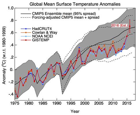
And that just isn’t true. I’ve updated the viewer here to show with latest data how Hansen’s predictions have stood up. I have superimposed in blue the index (Ts – met stations only) which is the one he was predicting. It is the index from Hansen and Lebedeff (1987). The scenarios A, B and C are showing. What has unfolded in GHG forcing is somewhere between B and C, closer to B. And GISS Ts has followed that closely. It lagged a bit around 2010, but has now overshot slightly, even exceeding Scenario A. I have shown the average of 2016 to end Oct; it will be a little lower by end year.
I have also shown the modern GISS version Ts+SST, IOW land/ocean, with SST, in brown. This has risen a little more slowly, and is now almost exactly on scen B. You can argue about whether it is tracking as closely as it should. But you certainly can’t say it is meaningless.
The ridiculously large errors claimed here are also refuted simply by the agreement of the various model projections. It isn’t perfect, but it isn’t the spread you would expect if the errors were 114 times the variable.
Nick writes
Then you dont understand what the video is about.
OK, Tim, please do tell. I’m reading Janice:
“26:46 — The error bars are larger than the temperature projection even from the FIRST year. The error is 114 times larger than the variable from the GET GO. Climate models cannot project reliably even ONE year out.”
I didn’t measure it myself, but it did seem to be what was said (very hard to be sure if people won’t put stuff in writing).
Nick wonders
The analysis shows not that the models haven’t “projected” vaguely correctly, it can be argued that they have when you just look at the graphs…but it shows that they cant have projected based on anything meaningful because the errors on clouds alone, when accumulated, wipe out any signal there may be.
So what’s left is a result of tuning. Which really means fitting against elements of climate that aren’t properly modeled. Clouds are an obvious one…
Nothing I can say will convince you of it, of course. But hey…one day Nick…
“but it shows that they cant have projected based on anything meaningful”
No, the projection worked. It is meaningful. You’re sayin g that follows from tuning. If so, it’s still meaningful.
But it doesn’t follow from tuning. Frank’s error analysis is just wrong.
Nick writes
In what way? Where is his error?
(reposted – as I’d somehow put it below)
Oh and
You know better than that.
“You know better than that.”
Nonsense. It’s a simple proposition, and anyone can see. Hansen made a projection nearly 30 years ago, and it has stood up well. That is meaningful. It doesn’t matter if PF claims it’s impossible. It happened. And for my part, I think Hansen got it right for the right reasons.
I’ve responded to your other (duplicate) below.
Nick is making the undergrad error that Pat explains at the end. The difference between systemic errors and physical errors. Go back and listen to the questions Nick.
Nick writes below (but lets bring it back up here
But he showed the errors were systemic. There is no cancelling.
And
No. A fitted projection will vaguely work if we continue to warm but it has no actual meaning. An analogy might be that the stock market tends to overall increase in the long term perhaps due to more new and improving businesses but you can never project what it’ll be at any given point because whatever method of projection you use, it has no basis in reality.
Nick writes
Re-watch it. He said he takes the average error of the variances and uses that to calculate his +-4W.
You said: No, the projection worked. It is meaningful. [Tim is] saying that follows from tuning. If so, it’s still meaningful.
What I heard from that: “The numbers are close, so the GCMs must be meaningful; even if it takes tuning to do it, being close enough that tuning helps still makes them meaningful.”
I could say the same thing about “projections” of my local surface air temperature based on throwing at a dart board or rolling a 20-sided die, with “tuning” to account for seasonal variation, lat/long., etc. The fact that a large percentage of my “projections” & actual observed temperatures will be within a narrow distance of one another doesn’t mean I’ve found something meaningful about the relationship between dart-throwing and weather forecasts. It just means the two number sets happen to overlap — and that’s it.
Just so we’re clear, I’m NOT trying to compare the average GCM to a random d20 roll or throw of darts, per se, even facetiously; I AM trying to say that, based on Frank’s presentation, the current GCMs may be little more relevant than such ‘random’ number generators to the actual prediction/projection of future climate, despite their complexity. Judging from the presentation, one might even be persuaded to think it a strong probability at this point.
Put more simply, & in another way: creating a computer model which predicts that Alabama will beat Florida 61 – 48 (or vice versa; FL can win 70 to -2 for all I care) is all very well, and looks pretty impressive if the actual result ends up AL-59 to 46- FL… but what does it really mean if the two teams were actually playing basketball when the model programmers THOUGHT the two teams were playing football?
Stokes,
You said, “And for my part, I think Hansen got it right for the right reasons.” Your belief may be misguided. One of the greatest intellectual ‘sins’ is to be right for the wrong reason. It isn’t sufficient to just believe that Hansen got it for the right reason. One might easily complain that Hansen’s prediction is no more than a spurious correlation. TTTM has suggested that Hansen’s predictions are the result of tuning, and not that the underlying physics are correct. I think that you have to demonstrate that TTTM is wrong and PF is wrong. So far, you haven’t presented what I would accept as a compelling argument for either.
Oh come on. Were the GCMs run in 1960? So amazingly they handcart accurately when tuned to handcart accurately. Pointless to show that part if the graph, and deliberately misleading. And a sharp spike probably due to a big El Nino now makes the GCMs accurate? If you can’t be honest about this, we have to assume the GCMs are not working. Otherwise why fudge and mislead?
“Were the GCMs run in 1960?”
No, Hansen’s GCM was run (for the 1998 paper) during years 1983 to 1987. But as usual, they ran for a long time on historic forcings to set the state for recent and present (1988).
There was a much criticised period from about 2000-2014 when the predictions seemed a bit warmer than observed. Now they are quite a bit cooler. That difference will reduce again. But the claim here is not that there are discrepancies, but that the Hansen projection is meaningless because of claimed huge errors. And that is clearly not so.
Exactly Nick:
Just the usual from the usual here.
“Post-truth” indeed and if it wasn’t for you and Leif, and maybe me and a few others, then, we’d just have the fan-boys cheering on the the “post-truthers” (vis “non-technically trained person” ) in the echo-chamber.
“(for what it’s worth)” . Worse than zero actually, when combined with ideological bias.
Toneb writes
And you didn’t understand the video either.
I do not know about the rest but HadCRUT4 is only four years old. (Morice et al. J. Geophys. Res. 2012) So it couldn´t have been used for hindcasting. And if HadCRUT4 has not used in hindcasting it cannot be used to validate the model.
Funny how the hi cast predicts golcanic activity, yet it isn’t tuned to match the past.
Omg auto spell check
Hind not hi
Volcanic not golcanic
Should probably use the actual base periods rather than recenter on 1990.
Nick writes
In what way? Where is his error?
As someone noted above, he adds variances but doesn’t divide by N. Actually I think the error there is more subtle. But he did a similar analysis here. That at least was in writing. It concerned surface indices, and again claimed that they were subject to huge errors. Basically he refused to acknowledge the effect of cancelling. But again, that flies in the face of common knowledge. SATs are not meaningless. People here are discussing them all the time. Different folks, including me, calculate them, and they agree. People here make all sorts of arguments about their meaning. Not always to good effect, but very few seem to think they have the kind of error overlay that Pat Frank asserts.
I’m certainly not going to give any credit to this very similar analysis until I see it in writing.
Nick, “As someone noted above, he adds variances but doesn’t divide by N.”
The propagated uncertainties are not averages, Nick. There’s no reason to divide by N.
Nick, “But he did a similar analysis here.” No, I did not. That was a different approach entirely, which in fact did involve taking averages. The problem for you there, is that the systematic error averages as rms, and does not diminish as 1/sqrtN.
“Basically he refused to acknowledge the effect of cancelling.” Wrong again, Nick. You completely failed to understand that limited instrumental resolution introduces errors into measurements. Those errors result in incorrect rounding. The measurement errors are then transmitted right into the average, proper rounding notwithstanding. It seems you never got that point.
You wrote, “Different folks, including me, calculate [SATs], and they agree.” Sure. They are the same data and all have the same systematic errors.
The “error overlay” I used has been reported in the literature from sensor calibration experiments, Nick. The systematic errors are known and known to be large. I’ve merely applied them to the global record, which no one else has seen fit to do.
You wrote, “I’m certainly not going to give any credit to this very similar analysis until I see it in writing.”
It’s not a similar analysis. It’s a different analysis.
Uncertainty in the SAT is rmse. Propagated uncertainty in air temperature projections is rsse. The analysis varies with the sort of data being assessed. They both deal with the large systematic errors contaminating the data. But that is beside the point you intend.
Nick, Hansen’s ‘prediction’ ignores the facts that disproves CAGW, that disproves AGW. If observations disprove a theory, the theory in question predictions are pointless.
Whether the planet will or will not warm or cool in the future has nothing to do with anthropogenic CO2 emission.
There is observational evidence that greenhouse gases cause no warming which is a paradox. A paradox is an observation that is not possible if a theory is correct.
There is a reason the cult of CAGW talks on and on and on the warmest year in ‘recorded’ history. ‘Recorded’ history is the temperature in the last 150 years. There is a reason every CAGW ‘presentation’ is a monologue with restricted scope.
1) Latitudinal warming paradox (the corollary of the latitudinal warming paradox is the no tropical tropospheric hot spot paradox) i.e. Global warming is not global.
2) The earth has warmed and cooled in the past paradox
It is a fact that the earth cyclically warms and cools, with the majority of the warming occurring at high latitudes. It is also a fact that solar cycle changes correlate with past cyclic warming and cooling of the planet.
The warming that has occurred in the last 150 years is primarily high latitude warming.
As CO2 is evenly distributed in the atmosphere and as the most amount of long wave radiation emitted to space is at the equator, the most amount of ‘greenhouse’ gas warming should have occurred at the equator.
There is cyclic warming in the paleo record both poles.
3) The lack of correlation in the paleo record
For example, there are periods of millions of years when atmospheric CO2 has been high and the planet is cold and vice versa. There is not even correlation in the paleo record.
http://wattsupwiththat.files.wordpress.com/2012/09/davis-and-taylor-wuwt-submission.pdf
I wonder what caused cyclic warming and cooling on the Greenland Ice sheet in the past? Curious that the same periodicity (time between events, 1500 years with a beat of +/- 400 years) between all warming and cooling events/cycles (including the massive ‘Heinrich’ Event is the same (same periodicity, same forcing function). It is also really weird that the warming and cooling periodicity is observed in both hemisphere.
Greenland ice temperature, last 11,000 years determined from ice core analysis, Richard Alley’s paper. William: As this graph indicates the Greenland Ice data shows that have been 9 warming and cooling periods in the last 11,000 years.
http://www.climate4you.com/images/GISP2%20TemperatureSince10700%20BP%20with%20CO2%20from%20EPICA%20DomeC.gif
oh my god, CO2 has an negative correlation wit air temperature!!1!
I theorize that we will all freeze to death. in 2100.
The entire scientific basis in the IPCC reports is incorrect. The IPCC reports are propaganda (see climategate emails). The IPCC reports for example did not include the long term paleo record (temperature last 11,000 years which shows the planet has warmed and cooled cyclic, same high latitude warming, and the planet was roughly 1C to 1.5C warmer during this current interglacial.)
1) Latitudinal temperature paradox (Strike 1)
The latitudinal temperature anomaly paradox is the fact that the latitudinal pattern of warming in the last 150 years does match the pattern of warming that would occur if the recent increase in planetary temperature was caused by the CO2 mechanism.
The amount of CO2 gas forcing is theoretically logarithmically proportional to the increase in atmospheric CO2 times the amount of long wave radiation that is emitted to space prior to the increase. As gases are evenly distributed in the atmosphere the potential for warming due to the increase in atmospheric CO2 should be the same at all latitudes.
http://arxiv.org/ftp/arxiv/papers/0809/0809.0581.pdf
As the amount of warming is also proportional to amount of long wave radiation that is emitted to space prior to the increase in atmospheric CO2, the greatest amount of warming should have occurred at the equator.
There is in fact almost no warming in the tropical region of the planet. This observational fact supports the assertion that majority of the warming in the last 50 years was not caused by the increase in atmospheric CO2.
http://www.eoearth.org/files/115701_115800/115741/620px-Radiation_balance.jpg
2) The planet cyclically warms and cools with the majority of the temperature change occurring at high latitudes. (See Greenland ice sheet temperature above last 11,000 years).
“2) The planet cyclically warms and cools with the majority of the temperature change occurring at high latitudes. (See Greenland ice sheet temperature above last 11,000 years).”
Err, it’s obviously escaped your notice, but Greenland is not “the planet”.
Neither is high latitude plateau with average temps ~ -30C in any way a proxy for it.
And BTW: this is what it would look like updated with modern temps.
(The Alley graph ends in 1855 – before any modern warming began)
http://2.bp.blogspot.com/-hksiecM4u3Q/VLYC3ecYOKI/AAAAAAAAAP4/ZsJFpmrxgZo/s1600/GISP2%2BHADCRUT4CW%2BHolocene.png
“And BTW: this is what it would look like updated with modern temps …” (Toneb).
================================================
That is a ridiculous comment, the red trend line is at a much higher resolution than the Alley graph.
Besides the peak around 1940 could not possibly be due to human CO2 emissions which according to the US Carbon Dioxide Information Analysis Center (CDIAC) were relatively negligible prior to ~1950.
And besides a highly smoothed time series graph should never be extended beyond its formal limits.
“That is a ridiculous comment, the red trend line is at a much higher resolution than the Alley graph.”
No, sorry the Alley graph does NOT show modern warming.
Anthony knows that, as it is in the “Disputed graphs” section here.
Now why didn’t you?
https://wattsupwiththat.com/2013/04/13/crowdsourcing-the-wuwt-paleoclimate-reference-page-disputed-graphs-alley-2000/
NB: That page is from April 2013, so add on the last 4 years of warming from GISS.
(~0.3C).
Christopher:
Could you please give me a solitary (as at a single geographic location) proxy that you would accept in the “hockey-stick”…… for the Globe.
Exactly.
This is a link to a graph that shows the amount of short wave radiation (sun light) that strikes the earth by latitude and the amount of long wave radiation that is emitted by the earth also by latitude.
The link I provided above to the same graph did not work.
http://www.physicalgeography.net/fundamentals/images/rad_balance_ERBE_1987.jpg
The correspondence doesn’t mean a physical thing, Nick. The underlying uncertainty is hidden from view. See the discussion of that point around Figure 1, here. None of those projections represent unique solutions (or tightly-bounded solution sets) to the problem of the climate energy-state.
You could also find the same correspondence using a family of polynomials. Would the one with the best correlation to the observations have physical meaning? That’s your analysis, isn’t it. Correlation = causation.
And in light of your certainty, what do you make of this statement of Hansen’s “Close agreement of observed temperature change with simulations for the most realistic climate forcing (scenario B) is accidental, given the large unforced variability in both model and real world.” in Hansen, et al., 2006 PNAS 103(39), 14288–14293; doi: 10.1073/pnas.0606291103
He seems to disagree with you.
“You could also find the same correspondence using a family of polynomials.”
You could, after the fact. But Hansen was predicting, not fitting polynomials. And he got it right.
And his quote is certainly not agreeing with you that the prediction is meaningless. He’s just saying the very good agreement (in 2006) needs to be viewed with the (unforced, or natural) time variability of both curves. He isn’t saying that there is a large systematic error. In fact he’s refuting Crichton’s (14) claim of a 300% error:
“Close agreement of observed temperature change with simulations for the most realistic climate forcing (scenario B) is accidental,given the large unforced variability in both model and real world.Indeed, moderate overestimate of global warming is likely because the sensitivity of the model used (12), 4.2°C for doubled CO2, is larger than our current estimate for actual climate sensitivity, which is 3 ± 1°C for doubled CO2, based mainly on paleoclimate data (17). More complete analyses should include other climate forcings and cover longer periods. Nevertheless, it is apparent that the first transient climate simulations (12) proved to be quite accurate, certainly not ‘‘wrong by 300%’’ (14).”
And another decade of agreement reinforces that.
Nick writes
In what sense did he get it right? By presenting the different rates of warming and having reality be close to one of them? The fact its just not – by looking at the slopes, not the fact a single recent point appears to be near his prediction today.
TimTheToolMan: so if I understand it properly: the models are tuned to “predict” (retrodict?) past behavior, but since they do not accurately model the underlying physical processes cannot actual predict future behavior. Right?
Correct. GCMs dont get the most fundamental quantity right without tuning. The top of the atmosphere radiation imbalance doesn’t emerge from the models, its tuned to be what is believed to be the current imbalance. Nothing after that can have any meaning in terms of projection.
The propogated errors is equally damning. There are multiple reasons why models cant project accurately but people like Nick cant or wont see them for what they are. But then again Nick thinks a fit is meaningful so…what can you say?
Those projections are from a parametrized model, Nick. The parameters have been adjusted by hand. All the parameters have significant uncertainties. Those uncertainties were not propagated through the projections, and do not appear as uncertainty bars in the plotted projections. Presenting those projections without their uncertainty bars gives a false certainty, and is misleading and naïve at best.
Tuned parametrized models do not make predictions, because their expectation values are not unique solutions. Your entire argument turns on a statistically good correspondence. Statistics isn’t physics, Nick. Pretty much all of your arguments are grounded in the opposite misperception.
Nick, “It isn’t perfect, but it isn’t the spread you would expect if the errors were 114 times the variable.”
You can get that spread by adjusting parameters to offset their errors. Projections made using models with off-setting errors are not correct, even if they correspond with observations, because the underlying physics is wrong. I discussed that point extensively here.
Hansen’s Scenario A, B, and C projections fall under that criticism. They’re not unique solutions, they have huge but hidden uncertainties, and are therefore physically meaningless.
You wrote, “(very hard to be sure if people won’t put stuff in writing).” It’s in writing right on that slide. It presents the average annual change in CO2 forcing since 1979 as about 0.035 W/m^2. The annual average CMIP5 long-wave thermal cloud forcing error is ±4 W/m^2. The error is ±114 times larger than the perturbation. The projection uncertainty due to this error is hidden by offsetting parameter errors. to repeat: projections made using models with off-setting errors are not correct, even if they correspond with observations, because the underlying physics is wrong.
And that ±4 W/m^2 is only a lower limit of error.
“Tuned parametrized models do not make predictions, because their expectation values are not unique solutions.”
Actually Hansen did very little tuning. He couldn’t. There was almost no history of other GCMs to refer to, and he couldn’t do multiple runs himself. They took months.
“They’re not unique solutions, they have huge but hidden uncertainties”
You keep falling back on this notion that there are huge uncertainties, that somehow don’t appear in the results. I come back to this simple refutation. Hansen made a prediction. It was a unique prediction. Just one (OK, 3 for prescribed scenarios). And he got it right. Despite the allegation of noise that was 114 times the signal that he was seeking.
When you throw a die, you can predict the outcome in two ways:
1) You can guess it. Use probability theory to compute the odds of a correct prediction = one in six
2) Determine exactly the initial conditions and solve the equations of Newtonian mechanics to predict the outcome
I think climate models try to do 2 but end up getting 1 because the Navier-Stokes equations are analytically unsolvable so they run the models many times and the outcomes are analyzed statistically. It’s inverse probability or Bayesian inference. Some statisticians have serious doubt about this method but I guess it’s a little better than a random guess, even if the guess is correct by chance
In other branches of science we use empirical data to parametrize models, then we run the model and we compare the results to new empirical data measured in the same way as the data used to parametrize the model.
Apparently, that is not the case with climate models. Now you are telling us that Hansen did very little tuning. You cannot assure that real empirical data (temperatures) was used to parametrize the model, and, as we can see, global temperatures are getting adjusted all the time. (In 2012, the year 1998 was the warmest in recorded history according to HadCRUT3 but the third warmest according to HadCRUT4)
Nobody can tell now if the model works or not because they keep changing the way global temperatures are calculated.
It is worse than that. By adjusting global temperatures they are “helping” the die fall on the desired face.
Nick writes
And you’ve never quite grasped what that means. They’re a fit. They cant project with meaning. There is no climate signal present because its swamped with propagated error. Hansen’s projection has no meaning, he gave himself a huge range of possibilities so its little wonder reality fits somewhere in there given we’re warming.
“You cannot assure that real empirical data (temperatures) was used to parametrize the model, and, as we can see, global temperatures are getting adjusted all the time.”
People just can’t seem to drop the notion that GCMs are somehow programs for curve fitting to past temperatures. Where tuning is done, it’s usually in response to some measurand that directly relates to what is unknown – eg TOA flux balance and cloud albedo.
But in any case, there would have been little adjustment performed in 1988. Just getting the data was a major task.
And you say “You cannot assure” – well, I can. Like anyone, I can calculate the global average using unadjusted GHCN, and I do. It makes very little difference.
TTTM,
“And you’ve never quite grasped what that means. They’re a fit.”
Despite years of blog commentary, you still seem to have no idea of how GCMs work.
“Hansen’s projection has no meaning, he gave himself a huge range of possibilities so its little wonder reality fits somewhere in there given we’re warming.”
Three scenarios is not a “huge range of possibilities”. It isn’t a range at all. When you check later, there is only one. The scenario that is relevant is the one that happened. There is a little fuzz because what happened won’t exactly match any one of them. But that fuzz is nowhere the ridiculous claim of 114x noise.
Nick writes
I know how they work Nick, I’ve even examined some of the code.
The thing is that when you approximate a process in the model and tune it to represent what we know, then that’s fitting it. Not much, you might think…but when that process iterates millions of times the you lose the approximately correct right part to the accumulated error.
This problem applies to pretty much every area of the model, not just clouds.
Nick, tuning means adjusting parameters within their uncertainty bounds to get a model calibration run to match observations. One needn’t refer to a history of GCM runs to do this.
You wrote, “ It was a unique prediction. Just one (OK, 3 for prescribed scenarios).”
A single projection is not a unique prediction. A unique prediction results when the physical elements of the model are so well-bounded that only one expectation value, or a tightly bounded set of expectation values, is produced for a single input. Climate models are far from that standard.
Nick, “And he got it right. Despite the allegation of noise that was 114 times the signal that he was seeking.”
Hansen himself said scenario B correspondence was accidental, given model errors.
And it’s not noise that’s 114 times larger than the perturbation. It’s model error — specifically CMIP5 long wave cloud forcing error — that’s 114 times larger than the perturbation. That uncertainty due to that error is hidden by off-setting parameter errors.
That’s 42 minutes just to say that a 1% change in global cloud coverage would have a bigger effect than the CO2 increase since 1900. This has been said repeatedly, even by some climate scientists, to no effect. It shows that the climate change political debate has never been about what the climate of 2100 is going to be. The debate is about the policies, not about the climate. Fear and disinformation are used by every government that tries to impose policies for which there is no popular support, being them invading a foreign country or changing the energy landscape. It is all being done supposedly for our own good without explaining us the ultimate reasons because they are not acceptable.
Actually this is such old news that it was published in 2009 in the Skeptic magazine (vol 14, n. 1) inspiring the famous cover and creating a huge controversy in the Skeptic Society because apparently you can be skeptic of anything except climate change. If you want a written version of the talk in html or pdf format or want to take a look at his analysis, no need to wait for a scientific journal to accept his paper. You have it here:
http://www.skeptic.com/reading_room/a-climate-of-belief/
http://www.skeptic.com/wordpress/wp-content/uploads/v14n01resources/climate_of_belief.pdf
http://www.skeptic.com/wordpress/wp-content/uploads/v14n01resources/climate_belief_supporting_info.pdf
http://www.skeptic.com/magazine/images/magv14n01_cover.jpg
“apparently you can be skeptic of anything except climate change”
Yes, that’s what I told them when they asked me to extend my subscription and refused.
I also refused to renew after a trial subscription when I realized that the professional skeptics were devout members of the Church of AGW.
Thanks, Javier. 🙂 The Skeptic analysis used an earlier version of satellite global cloud data, and earlier climate models. Along with updates of those data, the present analysis rests on a more complete analysis of the treatment of CO2 within climate models.
Richard Betts’ job is Director of Climate impact assessment studies (sic) using a totally useless model on which to base those impacts.
Please will you close down these people and save tax money.
To be fair, the Met Office crew model is one of the better ones in that it fails less badly than most of the others. Richard Betts would be taking his career in his hands if he publicly said that the real scare stories are based on other models which should have been culled years ago. The scare needs the bad models to propagate the error (pun intended).
Thanks, Janice and Eric.
I’ve always found the graph on the left (a screen cap from Pat Frank’s presentation) and its explanation to be entertaining. They’ve taken model failings (the models are unable to simulate the contributions to warming of naturally occurring, naturally fueled coupled ocean-atmosphere processes, like ENSO, like the AMO) and turned those failings into “proof” that greenhouse gases are responsible for the observed warming.
Marketing at its worst, or best, depending on your point of view.
On the chart on the left, the blue line, representing the model results using only natural forcings, shows little or no warming since about 1850. Temperature reconstructions, such as those from Greenland Ice cores, show that the mid 1800’s were the coldest years in the last several thousand years. Considering the variability in the climate shown in those reconstructions, it is simply not plausible that we would get no natural warming from the cold of the little ice age.
The blue line in the chart on the left shows little or no natural warming since about 1850, which was around the end of the Little Ice Age and the coldest period in the last several thousand years. Considering the variability in the climate, it does not seem plausible that the earth would not recover from this cold period.
The graph on the left is also the result of circular reasoning because it is based on assumptions which it purports to discover.
An excellent post which needs publicising more and hence a small contribution here:
https://wolsten.wordpress.com/2016/11/23/a-climate-of-belief-by-patrick-frank/
I concluded:
“A secondary take out from his analysis is that his own simplified Model of Models simulates to a close approximation the results of all the existing publicly funded climate models at a tiny fraction of the cost. At the very least it would be better to throw every one of those expensive models away along with their supercomputer infrastructure and save tax payers a huge expense moving forwards. The results would still be meaningless but at least we could afford to fund some real research with the money saved.”
I was surprised by the slide showing that the climate models use a linear relationship between carbon dioxide in the atmosphere and warming. I had always seen a logarithmic relationship, with the effect of increased carbon dioxide decreasing with concentration. What am I missing?
It’s that CO2 forcing is linear with temperature, but forcing is proportional to the log of the CO2 concentration.
Nice analysis, but it still assumes that the software is basically error free. But as a software engineer, I have no faith in that assumption. In my experience, software written by non (software) professionals without a documented rigorous process (including design documents, code peer review, testing, v&v, etc.) is always buggy. Any many times in tricky, non-obvious ways. I wouldn’t trust such software any more than a non calibrated instrument. This is something that Nick Stokes and his friends can’t, and won’t address, but it is critical.
“This is something that Nick Stokes and his friends can’t, and won’t address, but it is critical.”
Spoken by someoe who understands software, but not what the software is calculating.
The software cannot be “buggy” (in the sense that it alters the calculation).
It is doing an integrated calculation.
And like the “butterfly”, the calculation would rapidly diverge with algorithm “bugs” present.
That trends show variability (ie wiggliness) is evidence that they aren’t.
Same with NWP.
Weather models to cannot be “buggy”.
They may have parameterizations that are imperfect.
But the physics is modeled without any bugs.
From: http://www.easterbrook.ca/steve/2010/04/climate-models-are-good-quality-software/
“The idea for the project came from an initial back-of-the-envelope calculation we did of the Met Office Hadley’s Centre’s Unified Model, in which we estimated the number of defects per thousand lines of code (a common measure of defect density in software engineering) to be extremely low – of the order of 0.03 defects/KLoC. By comparison, the shuttle flight software, reputedly the most expensive software per line of code ever built, clocked in at 0.1 defects/KLoC; most of the software industry does worse than this.”
Just like the Shuttle had errors, but crucially, didn’t have them where it mattered.
Sorry toneb, but a simple typing error can cause a “Bug” in any computer program or model..Period..
Toneb,
You obviously don’t understand software engineering. It does not matter what they are calculating. There are many types of errors which can cause small errors that would not necessarily make even a highly iterative process go off the rails, but would still invalidate the results. Some examples are: loss of floating point precision during calculations/conversions, unexpected truncation, violation of array boundaries, logic errors which don’t occur on every iteration, etc. This is why we have these processes (requirements, written design, code peer review, unit testing, full coverage testing w/MCDC, verification testing, full tracing from requirements to test, etc.). Over the last 30 years I have worked on many safety critical systems, including pacemakers (look up my patent if you doubt me) and air traffic control software. I have seen so many different ways to screw up software, both subtle and obvious, that I don’t trust anything that has not been developed under a rigorous, documented process.
So they “estimated” the number of defects in their code. Not good enough when you are using the models as a large plank in your argument to change government policy and change our entire energy infrastructure. These proposed changes will cost trillions of $ and affect the lives of billions of people. We must do better than just taking some process models and estimating the number of defects/KLoC and call it good because the results “look good”. Everything must be done properly, using current best practice, and transparently from start to finish for something of this magnitude. Nothing less should be accepted.
I don’t know what area of science or technology you work in (if any), but would you accept the results of an experiment or study that used hand-built, unverified and uncalibrated equipment?
So, we checked our own software and figured out it was better than the best money could buy?
“Sorry toneb, but a simple typing error can cause a “Bug” in any computer program or model..Period..”
Indeed it can – but in the case of the Shuttle software it wasn’t critical was it?
despite having 3x as many bugs/KLoC.
(Remember: “reputedly the most expensive software per line of code ever built”)
“I don’t know what area of science or technology you work in (if any), but would you accept the results of an experiment or study that used hand-built, unverified and uncalibrated equipment?”
Meteorologist with the UKMO 32 years.
And yes.
Just as the Shuttle Astronauts did.
(3x less “buggy”).
Toneb,
So, you would trust an unverified and uncalibrated measurement device, eh? Either you are a liar or an idiot, but in any case, it makes your opinions worthless. And you are not helping yourself by holding up the Shuttle program as some sort of standard. That’s just intentionally setting the bar too low. People died as a result of process failures there. And one of them was a school teacher that definitely did not understand the risks. We don’t need to repeat that on a massive scale.
Another point is that, if I understand what’s going on properly, they don’t actually model the underlying physics. See the discussion above about “engineering” vs “physical” models.
Even if the software is valid, the results are still irrelevant because they started with the bogus assumption that CO2 has a significant effect on climate.
“Even if the software is valid, the results are still irrelevant because they started with the bogus assumption that CO2 has a significant effect on climate.”
Nah, my friend – the hand-waving denial of the GHE of the only significant non-condensing gas in the atmosphere wont do with me, or science in general. You’d need to re-write 150 years of observation, experiment and discovery to do that.
Without it the Earth would approach -18C as a GMT pretty quickly.
http://www.giss.nasa.gov/research/briefs/lacis_01/fig2.gif
Sorry it just does despite the post-truth on display here.
Have a lookie here if you think that 0.04% is insignificant….
Addendum to graph above:
“Figure 2. Time evolution of global surface temperature, top-of-atmosphere (TOA) net flux, column water vapor, planetary albedo, sea ice cover, and cloud cover, after zeroing out all the non-condensing greenhouse gases. The model used in the experiment is the GISS 2°×2.5° AR5 version of ModelE with the climatological (Q-flux) ocean energy transport and the 250 m mixed layer depth. The model initial conditions are for a pre-industrial atmosphere. Surface temperature and TOA net flux utilize the left-hand scale.”
From: http://www.giss.nasa.gov/research/briefs/lacis_01/
Toneb writes
You really dont get it, do you.
Readers who are not familiar with this stuff,
“Have a lookie here if you think that 0.04% is insignificant….”
That’s ink in a small jar, and the man giving the demonstration is a con artist. He knows damn well it’s not like two blankets rather than one, if translated into the relative “greenhouse effect” those levels of CO2 in our atmosphere would result in. More like adding a sheet on top of a thick comforter. Toneb knows it too, I’m quite sure, but hey, gravy is good ; )
toneb – “Without it the Earth would approach -18C as a GMT pretty quickly.” That would require that the vapor pressure of water be zero or WV not being a ghg. Which of these are you not aware of?
“That would require that the VP of water be zero or water not to be a GHG”
Give me strength…..
No it would ONLY require that water be a condensing gas.
You do know how it is that water precipitates out of the atmosphere?
For the benefit of the ideologically challenged then…
By being cooled to it’s dew point.
When the temperature of air containing WV falls it condenses out its WV content.
You are aware of how fog forms or Cu/Cb cloud FI?
Now what is it that stops Cu/cb cloud from precipitating out all of its WV?
Answers on a post-card to Dan please.
Look -I know of your Sky-dragon slaying *physics* from Spencer’s place.
And you don’t get to make the world work the way you want it to.
Without NON-condensing GHG’s, the GMT of the Earth’s temp WILL fall away to -18C. It’s grey-body temp.
Why?
Because you cannot take out the 0.04% CO2 by COOLING the atmosphere.
Look it’s really not hard – and I will not stay in your rabbit-hole arguing empirical science with you.
Just use common sense will you.
“That’s ink in a small jar, and the man giving the demonstration is a con artist. He knows damn well it’s not like two blankets rather than one, if translated into the relative “greenhouse effect” those levels of CO2 in our atmosphere would result in. More like adding a sheet on top of a thick comforter. Toneb knows it too, I’m quite sure, but hey, gravy is good ; )”
Apart from knowing meteorology my friend, I also know that certain denizens are Sky-dragon slayers and refuse to accept empirically science.
Hint: look up “empirical’.
Do the experiment yourself.
Oh, while you’re at it, go look up the Beer-Lambert Law.
Go, on be a devil and learn some science.
The BL law involves path-length, so it’s worse than you think, as the jar was, what? 6ins thick, whereas the atmosphere is ~ 100,000x thicker than that.
If we could see only in terrestrial IR wavelengths, we would exist in a thick fog my friend.
Oh, and you may care (sarc) to look up “Ozone layer”, which is at a concentration of just 10 ppm.
And yet it has the insignificant effect of stopping the biosphere from frying via UV.
https://en.m.wikipedia.org/wiki/Ozone_layer
“…..In fact, without the protective action of the stratospheric ozone layer, it is likely that terrestrial life would not be possible on Earth, and that oceanic life would be restricted to relatively greater depths than those at which it can now comfortably occur.
http://science.jrank.org/pages/4974/Ozone-Layer-Depletion-importance-stratospheric-ozone.html
TaTa
Toneb,
Yes or no, please; Is CO2 doubling, more like going from one blanket to two, or like adding a sheet on top of a thick comforter?
Readers who are not familiar with this stuff (and those who are),
There was a very relevant discussion posted yesterday, that I believe will give you some idea just how much of a con that man giving the ink demonstration really is.
The Global Warming Hoax | Lord Monckton and Stefan Molyneux
JK:
“Yes or no, please; Is CO2 doubling, more like going from one blanket to two, or like adding a sheet on top of a thick comforter?”
The answer lies is the Beer-Lambert law.
(Involves path-length).
CO2 doubling is logarithmic. Each successive doubling causing the same increase in temp.
So the answer to your question is 2 blankets.
(Oh goody ; )
“CO2 doubling is logarithmic. Each successive doubling causing the same increase in temp.”
Correct; Each CO2 doubling causes the same increase (not a doubling of all previous increases.)
Therefore, this MUST be false, I say;
“So the answer to your question is 2 blankets.”
Sir, for your claim to be true, removing half the CO2 would need to remove the the whole of the metaphorical first blanket, and OBVIOUSLY that would not happen, right? Indeed there would still be the bulk of the current “greenhouse effect” warming from CO2 as there is now, right?
Pick a Temp T, say 20 degree C. Let’s say doubling CO2 causes a 1C rise. Start at 100ppm. Go to 200, and T goes up to 21C. Go to 400, T goes to 22C. 800, T goes to 23C. Don’t think of blankets, think of the “sensitivity” to doubling CO2.
“Sir, for your claim to be true, removing half the CO2 would need to remove the the whole of the metaphorical first blanket, and OBVIOUSLY that would not happen, right? Indeed there would still be the bulk of the current “greenhouse effect” warming from CO2 as there is now, right?”
Trying to see through that gibberish is not worth the effort my friend.
Some of us understand climate science on here.
Very few it must be said.
Ask Nick Stokes, of Leif Svalgaad, and Steven Mosher, just the few that can bother to get through the ignorance on here.
And then you’d still not take empirical science for being so.
“Ask Nick Stokes, of Leif Svalgaad, and Steven Mosher, just the few that can bother to get through the ignorance on here.”
If you think you can get some back up from any of those guys on your answer, go for it . . but I warn you, they’re all pretty smart . . ; )
toneb – “No it would ONLY require that water be a condensing gas.” That discloses your complete lack of understanding of vapor pressure. I suggest any engineering textbook on thermodynamics. Without this basic knowledge there is little hope of grasping how this works.
“When the temperature of air containing WV falls it condenses out its WV content.” Do you actually think that ALL of the WV condenses out? Another comment that demonstrates you don’t understand vapor pressure.
Have you never heard of the Clapeyron equation which relates vapor pressure to liquid temperature? Or simply looked at tables of vapor pressure vs liquid temperature (e.g. http://www.wiredchemist.com/chemistry/data/vapor-pressure ). Non condensing gases are not mentioned because they don’t make a difference.
Thanks for the link to Dan Miller’s YouTube video, Toneb. I had not seen it before. I’ve just posted a long comment on it, which I hope he notices. This is what I wrote:
Dan, this is an excellent demonstration of how a very small amount of dye can have a great effect on the absorption spectrum of a material. Anyone who has walked barefoot on a light-colored sidewalk on a hot summer day, and stepped from there onto a black asphalt road, can appreciate the effect that such a color change may have on temperature! But I have a few complaints about your presentation.
First of all, I think you should have used food coloring, instead of black ink, because that’s a better analogy to how CO2 works in the atmosphere. It works as a dye or colorant. CO2 only blocks certain wavelengths in the IR, like food coloring only blocks certain wavelengths in the visible. India ink blocks everything.
Second, at 2:05 in the demo, you mentioned that the second jar “is really only 28 parts per million,” which is correct. The syringe presumably contained 0.56 CC of 10% ink solution, and 0.56 ml in 2L of H2O = 0.56 / 2000 = 0.00028 = 0.028% = 280 ppmv. 10% of that is 28 ppmv, so you should have labeled the jar “28 ppm” instead of “280 ppm.”
Of course, if you’d really used 280 ppmv ink, it would have looked pitch-black, and it would have been indistinguishable from the 560 ppmv beaker.
That’s important to realize! Anthropogenic CO2 emissions have only a small effect on the Earth’s temperature, not because there is so little CO2 in the atmosphere, but because there is already so much!
From your demo, if a viewer believes the “280” and “560” labels, he probably gets the mistaken impression that 560 ppm CO2 will cause about twice the warming effect of 280 ppm. It won’t. CO2 has a logarithmically diminishing effect on temperature, and it’s already way past the point of diminishing returns. 560 ppmv CO2 will cause only about 10% more warming than 280 ppmv CO2 (between between 6% and 13%, depending on whose figures you believe).
Third, you failed to mention how the thickness of the Earth’s atmosphere compares to those beakers!
Although the atmosphere is less dense than liquid water, it is miles thick. The full thickness of the atmosphere is about the same mass as a 30 foot deep layer of water. Your beaker of water is only about eight inches wide. To get an equivalent thickness to the Earth’s atmosphere, you’d have to stack up about 45 of those beakers of water in a 30-foot-long row.
Now, if you were to look through (or shine a light through) the row of 45 beakers of colored water, imagine how deep the color would be, from just 28 ppmv food coloring or ink solution.
That’s why just a few ppmv of a trace gas, or even less, can significantly affect the spectrum of the light which passes through the Earth’s atmosphere, and have a potentially significant “greenhouse” effect.
Except at the fringes of carbon dioxide’s absorption bands, there’s so much carbon dioxide in the air that the atmosphere is already very nearly opaque to the IR wavelengths which carbon dioxide mainly blocks. So adding additional carbon dioxide has only a small effect. (MODTRAN Tropical Atmosphere calculates that just 20 ppmv of carbon dioxide would have fully half the warming effect of the current 400 ppmv.) Additional carbon dioxide still does have an effect, bit it is primarily on those wavelengths corresponding to the far fringes of carbon dioxide’s absorption bands, where carbon dioxide is nearly-but-not-quite transparent.
The best evidence is that the amount of warming in prospect from anthropogenic CO2 & CH4 is modest and benign. If we are fortunate, it may be sufficient to prolong the current Climate Optimum, and prevent a return to Little Ice Age conditions. (Aside: atmospheric physicist Wm Happer has discovered evidence that the warming effect of additional CO2 is probably overestimated by about 40%; see http://www.sealevel.info/Happer_UNC_2014-09-08/ )
Fourth, I wish you had mentioned that the Earth emits about as much radiant energy into space as it receives from the Sun. Most of your viewers are not scientists, and probably don’t realize that. If the Earth did not emit about as much radiation as it absorbs, it’s temperature would not be stable!
However, the incoming and outgoing radiation are at very different wavelengths. The incoming radiation is mostly shortwave: near-IR & shorter (visible, UV, etc.). The spectral peak for radiation from the Sun (i.e., for energy absorbed by the Earth) is around 500 nm. Here’s what the emission spectrum from the Sun looks like:
https://www.google.com/search?q=emission+spectrum+from+the+sun&tbm=isch
The outgoing radiation is almost entirely far-IR & microwave (i.e., longwave). The spectral peak for radiation from the Earth is nearly 20,000 nm. Here’s a good article showing emission spectra from the Earth:
http://wattsupwiththat.com/2011/03/10/visualizing-the-greenhouse-effect-emission-spectra/
So, anything in the atmosphere which has a different effect on different wavelengths has the potential to either warm or cool the Earth. If it blocks shortwave radiation but passes longwave radiation it will have a cooling effect. If it blocks longwave radiation but passes shortwave radiation it will have a warming effect.
For most wavelengths longer than about 4000 nm, the Earth emits more than it absorbs. For wavelengths shorter than that the Earth absorbs more than it emits. Conventionally, 4000 nm is near the boundary between near-infrared and mid-infrared.
If you were to “tint” the atmosphere with a colorant which blocks more incoming short wavelength (4000 nm) radiation, the planet would cool. But if you tint the atmosphere with a colorant which blocks more outgoing than incoming radiation, the planet will warm: that’s the so-called (but poorly named) “greenhouse effect.”
Greenhouse gases (GHGs) are colorants. They tint the atmosphere, but in the far-infrared, rather than the visible, part of the spectrum. Carbon dioxide and other GHGs act as dyes in the atmosphere, which “color” the atmosphere in the far-infrared (in the case of CO2, around 15 µm).
Since nearly all of the energy emissions from the Earth are in the far infrared & longer wavelengths, but over half of the incoming energy (from the Sun) is at shorter wavelengths (near infrared, visible & UV), tinting the atmosphere in the far infrared has a differential effect. Since there’s more outgoing than incoming far infrared, GHGs absorb mostly outgoing radiation, preventing it from escaping into space. That causes warming. (It’s not how actual greenhouses work, but it’s still a real effect.)
Greenhouse warming of the air, in turn, warms the ground, by a couple of mechanisms, including increased “downwelling” infrared back-radiation from the air.
There’s no legitimate dispute about this. We know how it works, and what it does, and we can measure the direct effects (such as downwelling IR). The only legitimate arguments are secondary: e.g., whether greenhouse warming is amplified or attenuated by feedbacks (and by how much), whether it is benign or dangerous, and what, if anything, can or should be done about it.
Here’s a good article:
http://barrettbellamyclimate.com/page8.htm
Isn’t the definition of non-trivial software that which contains bugs? 🙂
Yes. Unless it’s 1/2 million lines of mostly-sloppy, poorly-commented, mostly-antique, Fortran code. Then you’re a Science Denier if you don’t trust it as the basis for justifying “a roll-back of the industrial age.”
Good point, Paul. But one has to start somewhere. I’d be overjoyed if someone would subject the models to a full engineering analysis. Maybe some of the money Trump might save by stopping alt-Eng subsidies could be used to fully assess the models.
Background information (methods and such) of what is being discussed in the video can be found in the book Data Reduction and Error Analysis in the Physical Sciences by Phillip R. Bevington. https://www.amazon.com/reduction-error-analysis-physical-sciences/dp/B007EJ9DPI/ref=sr_1_3?s=books&ie=UTF8&qid=1479905490&sr=1-3&keywords=data+reduction+and+error+analysis+for+the+physical+sciences. This is a classic text for us physical scientists. Newer editions are available.
You’re right, Charles. That’s the reference I used; 3rd edition, Bevington and Robinson. 🙂
I once knew a mathematician who showed the government how their models were worthless because all results, no matter where they plotted, were equally valid/invalid. That person was never allowed to attend another meeting, as the bureaucrats and contractors continued with their work.
http://www.glasbergen.com/wp-content/gallery/math-cartoons/math_cartoons45.gif
Not Needle in a Haystack, more like Faeries on a Pin and it all started with the brief intro to Greenhouse Warming Theory and the magical 33 degrees.
as afr as radiation is concerned, we do not live on the surface of the Earth. we live under an atmosphere that is to all intents opaque to the infra-red radiation emitted by objects at (on average) 14 degC.
The atmosphere puts about 15psi of pressure onto us, or about 1kg per square centimetre or the equivalent of being under 1 metre depth of water or roughly one foot of dirt.
If you were a mole or earthworm or other critter at 12 inches underground, would you use a radiation analysis to work out the energy flows in your ‘environment’? Why?
Would a conduction & convection analysis not only be easier but more likely to yield the correct answer?
Is it not obvious that earth uses exactly that (we call it weather) in the troposphere until radiation takes over in the stratosphere, where weather effectively stops?
Sheesh! How many model “predictions” have to go wrong before their reliability is questioned by the “97%”?
Throw in how “reliable” the base data is (ie http://www.surfacestations.org/ , https://wattsupwiththat.com/2012/07/29/press-release-2/ ) and the only conclusion that can be reached is:
We don’t really know what the past temperature of the globe was but we can be certain that a computer model can’t can’t tell us what it will be.
The cause of any anthropomorphic warming? “The Cause”.
I’m sympathetic to this sort of analysis, but I think the error bar chart could be misleading. If the error due to cloud cover in any year is random within plus or minus 4 watts, then the probability of an error of + 4 watts every year is extremely small. Smaller net errors over the years will be more likely than large ones, as negative errors in some years cancel out (to some extent) positive errors in others. It would be helpful to see a chart with the probability of a cumulative error (in degrees centigrade) as a function of the size of the error.
David, the ±4 W/m^2 statistic represents a systematic error not a random error. It’s the annual average of error for the tested CMIP5 models. The propagated uncertainties are representative. An uncertainty statistic is not error, which is a physical magnitude.
Physical errors combine as their sign. However, physical errors are not known in a futures projection, so all one has to gauge predictive reliability is the uncertainty from propagated known errors.
“David, the ±4 W/m^2 statistic represents a systematic error not a random error. It’s the annual average of error for the tested CMIP5 models.”
That is the basic confusion here. If it’s systematic, then why is it ± ?
In fact, I can’t see such an error quoted by Lauer and Hamilton, and I don’t think they could, since the uncertainty of the observations is ±5-10 W m⁻². What they say is:
“For CMIP5, the correlation of the multimodel mean LCF is 0.93 (rmse ± 4 W m⁻²) and ranges between 0.70 and 0.92 (rmse ± 4–11 W m⁻²) for the individual models. “
It seems to be the rmse (root mean square error) of a correlation, not a systematic error.
Nick, “That is the basic confusion here. If it’s systematic, then why is it ± ?”
Because it’s the root-mean-square statistic of the annual average of individual model systematic error.
“It seems to be the rmse (root mean square error) of a correlation, not a systematic error.”
See their equation (1), page 3831, where they describe the error calculation: “A measure of the performance of the CMIP model ensemble in reproducing observed mean cloud properties is obtained by calculating the differences in modeled (x_mod) and observed (x_obs) 20-yr means. These differences are then averaged over all N models in the CMIP3 or CMIP5 ensemble to calculate the multimodel ensemble mean bias Δmm, which is defined at each grid point as Δmm = (1/N)[sum over N of (x_mod minus x_obs)] (1).”
With regard to the Taylor diagrams of error, they write that, “the linear distance between the observations and each model is proportional to the root-mean-square error (rmse)…”
Lauer and Hamilton also note that long- and shortwave cloud forcing errors are much smaller than the errors in total cloud amount or in liquid water path (unit area mass of liquid water droplets in the atmosphere). They ascribe the lower error to modelers focusing their model tuning to minimize the cloud forcing errors, so as to attain top of the atmosphere energy balance.
That rather makes the ±4 Wm^-2 a lower limit of a lower limit of model tropospheric thermal flux error.
“See their equation (1), page 3831”
That is an equation for bias. And it is simply added. No RMS.
“With regard to the Taylor diagrams of error, they write that, “the linear distance between the observations and each model is proportional to the root-mean-square error (rmse)…””
That quote refers to ‘the standard deviation and linear correlation with satellite observations of the total spatial variability calculated from 20-yr annual means. ‘
They are talking about the (spatial) sd of each model wrt its own mean, and correlation (not difference) with satellite. There is no “systematic error” there, and no time sequence as you have it. And that is what the 4 W m⁻² comes from. It is a measure of spatial variability.
Nick, calling your attention to eqn. (1) was just meant to show that Lauer and Hamilton calculated the difference between observed and modeled cloud properties. Not between model and model. The multi-model annual error statistic is calculated as the rms error of all the individual model errors relative to observations.
It is the inter-model cloud error correlation matrix I showed that demonstrated that the cloud error is systematic. Systematic error propagates through a serial calculation as the root-sum-square of the errors in each step.
I wrote, ““With regard to the Taylor diagrams of error, they write that, “the linear distance between the observations and each model is proportional to the root-mean-square error (rmse)…”
To which you replied, “That quote refers to ‘the standard deviation and linear correlation with satellite observations of the total spatial variability calculated from 20-yr annual means.”
No, it does not. Here’s what L&H say about the diagrams (p. 3833): “The overall comparisons of the annual mean cloud properties with observations are summarized for individual models and for the ensemble means by the Taylor diagrams for CA, LWP, SCF, and LCF shown in Fig. 3. (bold added)”
That makes it pretty clear that the Taylor diagrams represent model error.
They go on to write, “ These give the standard deviation and linear correlation with satellite observations of the total spatial variability calculated from 20-yr annual means.” indicating that the correlations are between model simulation and satellite observations; not correlations between models, nor individual models vs. model mean.
You wrote, “They are talking about the (spatial) sd of each model wrt its own mean, and correlation (not difference) with satellite.”
Given the quote from L&H above, they are doing no such thing.
You wrote, “There is no “systematic error” there, and no time sequence as you have it. And that is what the 4 W m⁻² comes from. It is a measure of spatial variability.”
Here’s what Lauer and Hamilton say on page 3831 about how they calculate cloud forcing (CF), “The CF is defined as the difference between ToA all-sky and clear-sky outgoing radiation in the solar spectral range (SCF) [shortwave cloud forcing] and in the thermal spectral range (LCF) [longwave cloud forcing]. A negative CF corresponds to an energy loss and a cooling effect, and a positive CF corresponds to an energy gain and a warming effect.”
From that, it is very clear that the ±4 Wm^-2 is not a measure of spatial variability.
The LCF is a thermal energy flux, and the ±4 Wm^-2 rmse of the simulated LCF is the mean model simulation error statistic in that thermal energy flux. It represents the mean annual simulation uncertainty in the tropospheric thermal energy flux, of which energy flux CO2 forcing is a part. That was how I used it in my error propagation.
Dr. Frank does an excellent job of presenting the statistical situation, without losing the audience with the fine detail that only the well-versed statistician would understand. In other words, the perfect level for the “informed” layman. I would really like to see more analyses at this sort of level, of all the impressive sounding stats that are bandied about by the climate elite. The 97% consensus has been well covered, but how about all these claims of 95% certain etc. that spew forth from the IPCC and get reported ad nauseum by our ignorant activist politicians and MSM as carrying some sort of great weight, simply because they sound near enough to 100%.
A major problem is that across the board (almost) government research money has gone exclusively to “scientists” dedicated to the mission of proving that AGW exists and is a major threat to mankind. Any deviation from that conclusion results in a cut off of funds and blackballing by the “peer review” process.
An apt analogy would be the Joyce Foundations history of funding gun safety “studies” with over 50 million $ provided exclusively to researchers committed in advance to anti-gun conclusions.
Another would be the cosmology community with everyone arguing that 99.4 % of the universe consists of “dark matter” which cannot be seen, measured or even proven to exist – now or literally ever. The “proof” is a hundred layer deep accumulation of mathematical scab patches to an originally empirically false theory.
If the theory doesn’t fit reality the proper next step is to adjust the theory, not adjust reality. Just a layman’s view, but the official government agencies “correction” of past temperature records is proof that at least the upper management of the agencies are nothing more than political hacks.
Dr. Frank – your cloud error analysis is based on an annual cloud error. Since the climate models are attempting to predict global temperatures out dozens of years would it make sense to do a cloud error budget based on a 5 or 10 year moving average of the cloud errors? If so how would that impact your conclusions?
Mike, the annual cloud error is the average from 20 years of calibration runs of 26 CMIP5 models. So, it really is the annual mean of a multi-year, multi-model set of results. Is that pretty much what you had in mind?
Yes thanks for clarifying
Pat Frank provided a very educational blog post and supported the discussion of it throughout the comment period so far. I am very appreciative of those commentators that do that give the amount of their time it requires. During the comment period on WUWT is where I learn the most about topics and usually make up my mind about the blog post. Although I have some background in statistics, error and reliability engineering, I have not used the background very much since college. This discussion brought back memories of long forgotten classes. I also took the time to look at references and read more on the topic of error propagation. My opinion after doing that is Dr. Frank won the argument with Nick Stokes. For what it is worth, I believe Dr. Frank is correct. The IPCC climate models are not useful in predicting future climate.
“Ensemble Average” : if I have two models, one totally wrong and the other fairly good, but I don’t know which is which. It does not seem to make any sense to calculate an Ensemble Average of this set of models. An it makes even less sense to use this average as a “consensus predictor”.
Hansen predictions of 1988 were fairly well within the ±14 °C error margin; this doesn’t validate his model.
Willie Soon alerted a number of people about the November 9 Carbon Brief (Clear on Climate) website post, presenting a series of interview videos and comment of climate scientists, bemoaning the election of Donald Trump: “US election: Climate scientists react to Donald Trump’s victory. There’s a lot of upset, anger, and anguish.
I posted a short comment and a link to the head-post presentation. Christopher Monckton quickly became embroiled in debate there, and, well, so did I.
But I discovered the comments were closed before the debate was resolved. So, if the moderator allows, I’d like to post a couple of replies here. Perhaps the pingback will bring the debaters here.
BBD you wrote, “You have jumped from the topic (global warming trend) to a non-topic (regional climate effects) invalidating your (but not my) argument. I never made any claims about the regional predictive skill of the models as that was not the focus of discussion. Don’t play crude rhetorical games, please.”
Apparently you don’t realize that localized precipitation is the mechanism for global heat transfer across the top of the atmosphere; a critical control element of the tropospheric thermal content driving air temperature. “crude rhetorical games” indeed. Merely central to your knowledge claim concerning AGW.
But let’s cut to the chase, shall we?
You claim your “greenhouse effect theory” explains the effect of CO2 emissions on climate.
For example, “As I keep telling you, this is about greenhouse effect theory not some ‘theory of climate’.” Except that the CO2 greenhouse effect on climate requires knowing whether there are any negative feedbacks. I.e., requires a theory of climate.
You do seem to have a problem distinguishing scientific knowledge from thus spake BBD.
You say your theory consists of radiation physics. Perhaps you consciously include the assumption of constant relative humidity. But that’s just the explicit part.
You apparently don’t realize there’s an implicit part of your vaunted “greenhouse effect theory,” that you’ve left unstated.
You assume no compensatory changes (negative feedbacks) in cloud cover or precipitation or IR radiative egress.
So, let’s itemize. Your “greenhouse effect theory” consists of radiation physics plus three assumptions left unstated.
That’s your “greenhouse effect theory.” It is a cryptic theory of climate, with hidden claims about the behavior of clouds, of precipitation, and about the rate of thermal energy flux through the top of the atmosphere.
The fact of your cryptic theory proves that a theory of climate is necessary to the full meaning of CO2 emissions on the climate; something you’ve repeatedly denied all the while implicitly hewing to it.
That you deploy a theory of climate, but do not yourself realize it, tells us all we need to know about your grasp of science.
Maybe seeing your implicit claims itemized will finally convince you of the scientific fatuity of your idea that radiation physics alone is a valid theory of the greenhouse effect; as though all other other parts of the climate were stationary.
Your position is an obvious crock, BBD. I suggest you follow up your own determination to “not be [it] saying again.” Such an ignorant display is embarrassing, even in a debate adversary.
You wrote, “Since sensitivity is an emergent property of model physics and not parameterised…” in the face of F.A.-M. Bender (2008) A note on the effect of GCM tuning on climate sensitivity Environmental Research Letters 3(1), 014001, from the abstract: “[This] study illustrates that the climate sensitivity is a product of choices of parameter values that are not well restricted by observations…” and R. Knutti, et al., (2008) Why are climate models reproducing the observed global surface warming so well? Geophys. Res. Lett. 35, L18704, p. 3 “Changes in model parameters (e.g., cloud microphysics) may result in compensating effects in climate sensitivity…”
After which you wrote, “You are a way outside your field of expertise…” One hopes your inadvertent irony is apparent even to you, BBD.
You’ve never grasped, or perhaps avoided, that my argument is about physical error analysis not climate physics.
You wrote, “Your entire argument collapses on the logical fallacy of appeal to your own (non-existent) authority and that is where it stops.” Wrong again, BBD. I’ve rested my argument on the scientific merits. Merits, let’s note, that you have conspicuously failed to address. You have yet to mount one single analytical point of objection. You’ve offered nothing but vacuous dismissals, denials, and derogations.
You wrote, “There’s no evidence that there was anything even approximating to a formal review process [to my Skeptic article]. Are you prepared to post all reviewers’ comments here?”
You’re welcome to contact Michael Shermer and ask about his process. You’ll find a direct debate about the article with Gavin Schmidt of NASA GISS here. Search my name. If you read to the end, you’ll find that I carried the debate. Gavin was reduced to accusing me falsely of a log(0) error that does not exist in my work.
I have posted on the quality of my reviewers’ comments here. Help yourself. None of them have indicated any understanding of the meaning of uncertainty derived from physical error. One of the Skeptic article reviewers distinguished himself by accusing me of scientific misconduct. You can read all about that false charge in the article SI (892 kb pdf).
You wrote, “Your (false) claim was that models alone were the source of our knowledge of the effects of CO2 forcing on climate.” And so they are, deploying as they do the relevant climate physical theory.
The above analysis shows that you, too, ‘claim that models alone [are] the source of our knowledge of the effects of CO2 forcing on climate,’ because you yourself deployed an implicit climate model. Except that you didn’t know it. By now you should have figured that out, though I doubt you’ll ever permit that understanding.
You wrote, “To be specific (because you have since tried to obfuscate the point) [the effects of CO2 forcing on climate] meant the effect of CO2 on GAT on centennial timescales. I pointed out that this was evident from palaeoclimate behaviour and that you were wrong.”
On the contrary, BBD. You never met the challenge that the resolution of the PETM data cannot support your claim. You merely assert it. Bald assertion is all you’ve done. Bald assertion is no proof. It’s just more thus spake BBD.
You also wrote, “You still are and now you are lying about it.”
I’ve lied about nothing. Once again you assert baldly and without evidence. And let everyone see your resort to character assassination when you cannot argue the evidence.
You wrote, “You can’t tell that WUWT is bullshit and most of CA is wrong? You are beyond help then.”
Yet another claim for which you’ve provided zero evidence. Just yet more of your thus spake BBD positivity.
Lionel Smith, your dismissal has no substantive content. You’ve merely accepted the mistaken claims of contradiction at Tamino’s “Frankly Not” at face value, with no evidence that you understand the argument. Or that there was no contradiction, as I showed.
You have every right to accept an infallible AGW priesthood, but don’t expect to get very far with it in a debate about science.
No one at Tamino’s “Open Mind” (irony alert), ever figured out that the cosine analysis of the global air temperature record was supported by an observed cosine residual in (T_land-surface minus T_sea-surface). Neither have you.
You “suggested reading Bradley wherein is described the varied methods of dendrochronology data collection and research [which] should answer your issue with my, supposedly, not providing the ‘physical theory Bradley uses to get temperature’”
No supposedly about it. You provided no physical theory linking tree rings and temperature. Neither has Raymond Bradley.
I fully understand that Bradley’s paleo-temperature reconstructions strictly employ statistics alone. They are based on no physical theory. The “temperature” numbers he elicits therefore have no physical meaning.
You reject that obvious conclusion. Faith in your priesthood again.
You wrote, “The comment thread at Real Climate ‘What the IPCC models really say’ is replete with similar criticisms of lack of coherence in your arguments.”
Criticisms I showed were incorrect. But you apparently passed over my demonstrations.
Gavin finally supposed I made log(0) error. That was his only remaining criticism. However, the regression stopped at log(1) = 0, something Gavin apparently never figured out. You merely quoting a series of replies supporting Gavin’s incorrect claim is no rejoinder.
The rest of your post supposes that AGW is causal to the current turmoil in the middle east. There’s as much evidence for that as there is of human-caused global warming itself.
Almost forgot — thanks, very much Mod, for allowing those responses. 🙂 I truly do appreciate it and am grateful.
Pat
Thank you Pat Frank.
Thanks right back, Roy. Your positive interest is appreciated.