Guest Post by Willis Eschenbach
I’ve been investigating the use of the “complete ensemble empirical mode decomposition” (CEEMD) analysis method, which I discussed in a previous post entitled Noise-Assisted Data Analysis.
One of the big insights leading to modern signal analysis was the brilliant idea of Joseph Fourier. He realized that any given waveform can be expressed as a combination of sine and cosine waves. However, there are other ways besides Fourier’s method to decompose a signal, including periodicity analysis, principal component analysis, and CEEMD.
Let me give you an example of a CEEMD analysis. Here are the intrinsic modes for the annual average number of sunspots from 1700 to 2014. The top row is the sunspot data itself. For intercomparison with other signals, it is standardized to a mean of zero and a standard deviation of one.
 Figure 1. CEEMD analysis of the mean annual sunspot numbers. Top panel shows the sunspot data, standardized to a mean of zero and a standard deviation of one. Panels marked C1 – C7 show the intrinsic modes of the signal. The bottom line shows the residual, meaning what remains after the removal of modes C1 – C7 from the signal. Note that all intrinsic modes are displayed at their true size, with all scales being the same.
This is a “complete decomposition” of the raw data signal, meaning that if we add the intrinsic modes C1-C7 together plus the residual, it will faithfully and exactly reconstruct the original signal.
One thing I like a lot about the CEEMD analysis is that I can actually see how the underlying intrinsic modes vary over time. I’ve said before that ascribing an inherent cyclical mechanism to natural observations is fraught with problems. Figure 1 is a good example of these problems. Look at intrinsic mode C4. It has a small signal at about 22 years … but not all of the time. For most of the first century of the record there is little signal at all. Then there’s an intermittent small ~ 22-year signal from about 1780 to 1850 ,,, which fades out and after a few year hiatus is replaced by a single ~ 25-year cycle, and that in turn is replaced with a ~ 22-year cycle out to the end of the data.
Or we can consider intrinsic mode C6, which varies in a similar irregular fashion. Mode C6 has a couple of strong cycles with a period of around 90 years at about 1800, and it then kind of tails off to nothingness. This makes it obvious why it has been so hard to discuss the existence or non-existence of the so-called “Gleissberg Cycle”, which Gleissberg claimed was ~ 80 – 100 years. When cycles come and go like that, it is hard to draw any firm conclusions. I mean, the ~ 80 – 100 year cycle is definitely there … but it’s only there when it is there, and the rest of the time, well, it’s simply not there.
Unfortunately, these kinds of appearing and disappearing cycles are far too common in natural datasets. There is a great temptation to think that they can be used for forecasting purposes … and they could if we ignore Murphy’s Law, which says that as soon as you start prophesying, the cycle will die out. For example, if we looked at the sunspot data in the year 1900, we’d think that there was a strong, statistically significant hundred-year cycle in the data … but after 1900 the cycle simply fades out to nothing.
Having seen the actual waveforms of the intrinsic modes in Figure 2, we can look at the periodograms of the various intrinsic modes to see what kind of signals exist in each of the intrinsic modes C1 to C7.
 Figure 2. Periodograms of each of the intrinsic modes C1 through C7 of the annual mean sunspot number, 1700-2014. These show the strength of waves of the various periods in each on the intrinsic modes.
Figure 2 shows that most of the energy is in the ~11 year cycle, which is in intrinsic mode C3. Because the sunspot cycle varies between ten and thirteen years, the energy is not a sharp spike, but has energy across that range.
As discussed above, intrinsic mode C4 can be seen to have a very small bit of energy in the 22 year range, but as we saw in Figure 1, there’s nothing regular enough in the data to give a strong signal.
Again as discussed above, intrinsic mode C6 seems to have some energy in the 90-100 year range … but as Figure 1 shows, the ~100 year signal in C6, while strong, is mostly visible in the first half of the data. This greatly increases the odds that it is a spurious signal that could disappear in a longer record.
So that is an example of a CEEMD analysis of a signal. It gives us a picture of the intrinsic modes (Figure 1) and the periodograms of those same intrinsic modes (Figure 2). It shows the strength and the ebb and flow of the underlying cycles in the data.
Now, how else can this kind of analysis be useful? Well, it can show whether and how two distinct observational datasets might be related. As an example, here is the CEEMD analysis of both the Nino3.4 Index and the Southern Ocean Index (SOI). The Nino3.4 Index is a detrended sea surface temperature dataset for an area in the tropical central Pacific covering 5° North to 5° South and 120° West to 170° West. The SOI, on the other hand, is an index of the atmospheric pressure difference between Tahiti and Darwin, Australia. The two indexes seem to be measures of the El Nino/La Nina pumping action. The SOI and the Nino3.4 move in opposite directions, so the SOI is usually displayed inverted so that peaks in the SOI correspond with peaks in temperature. The next two figures show the CEEMD analysis of the two datasets:

 Figures 3 and 4. Upper figure shows the intrinsic modes resulting from the CEEMD analysis of the Southern Ocean Index (SOI, red) and the Nino3.4 Index (black). These two datasets cover the same period as the sunspot data shown in Figure 1, 1870 – 2011.
Again, we see that there are various cycles which are strong in part of the record, but disappear or are greatly diminished in other parts of the record.
Note the close correspondence of the decomposition of the two signals, both in terms of the strength and shape of the intrinsic modes, and in their periodograms. It is clear that regardless of the fact that the Nino3.4 Index and the Southern Ocean Index are measuring different variables, they are both a measure of the same phenomenon.
And it is equally clear that there is no significant sunspot signal in either the SOI or the Nino3.4 data—the CEEMD analysis shows little commonality. Unlike the sunspot data, in the SOI and Nino3.4 data there is little strength at 11 years, and little strength at around 90 years. And again unlike the sunspots data, the majority of the energy is in the short-cycle (2-6 year) part of the spectrum.
Anyhow, that’s why I’ve grown fond of the CEEMD analysis … it shows when datasets have related cycles, and when they are unrelated.
Pushing towards full moon tonight, with Jupiter and Arcturus vying for the moon’s attention … what a world …
My best to everyone,
w.
My Usual Request: Misunderstandings bring communication to a halt, so if you disagree with me or anyone, please quote the exact words you disagree with so we can all understand your objections. I can defend my own words. I cannot defend someone else’s interpretation of some unidentified words of mine.
My Other Request: If you believe that e.g. I’m using the wrong method or the wrong dataset, please educate me and others by demonstrating the proper use of the right method or the right dataset. Simply claiming I’m doing something wrong doesn’t advance the discussion unless you can tell us how to do it right.
Yearly Sunspot Data: SILSO
SOI Data: Here
Nino3.4 Data: NOAA
Code: I’m using the “CEEMD” function in the R package “hht” for the analysis.
Very nice, Willis.
The 11-year ‘peak’ has two smaller peaks, one on each side of the main peak. These could be interpreted as modulation by a longer period [the ~100-year coming-and-going cycle].
Thanks, Leif. I don’t think that the 11-year cycle is being modulated by the 100-year cycle, although anything is possible. I say this because the CEEMD analysis method functions as a bank of empirically selected bandpass filters. As a result, the empirical mode that contains the ~ 11-year cycles (intrinsic mode C3) will not show the effects of the ~ 90-year cycles shown in intrinsic mode C6.
Or that’s my naive view, so now, I need to go and test it … hang on … … well, I made some synthetic data and ran a CEEMD analysis on it. I couldn’t make the intermittent 90-year cycle interfere with the ~ 11-year cycle, but that may reflect my own inability.
w.
Back when we were discussing the influence of planets, I showed that an amplitude modulation of the sunspot cycle by a ~100 yr cycle could generate the side peaks:
http://www.leif.org/research/AGU%20Fall%202011%20SH34B-08.pdf
Willis, what Dr. S is saying makes sense to me. If you have an 11 year “carrier” period, that is amplitude modulated by a longer period modulation, you should get upper and lower sideband frequencies on each side of the carrier as he suggests (well what he said suggests that to me.)
The presence of ‘noise’ in the signals (lucky us), well fluctuations could make it not nice and symmetrical as a spectrum, but his idea is a plausible explanation.
In any case, what you are doing, seems to be an interesting tool. I’m sure the mathematicians would likely want to know something about the boundaries of validity of such machinations; but if they have misgivings, then let them tell us about it.
G
Upper and lower sideband information is a standard part of amplitude modulation of a fixed frequency carrier.
Transmission of the accurate signal requires a transmission path bandwidth that incudes the upper and lower sidebands. It’s been a long time , but I believe each sideband is phase shifted from the carrier, and I think the two sidebands are either 90 degrees apart or 180.
in principle ALL of the modulation information content is contained in the sidebands; the carrier contains NO information (other than the frequency).
So it is common to suppress the carrier, to save transmitter power, and just transmit the sidebands (still need the same spectral width). In fact the two sidebands are supposed to be identical, at Fc + FM and Fc – FM, so you only need one of the sidebands, which immediately halves the spectrum width. That of course gives you suppressed carrier single sideband transmission, which is a very efficient AM modulation system.
Well, in reception, you need to know the carrier, both in frequency and phase, so the carrier power is just depressed, rather than eliminated, so the receiver can find a signal to lock onto to replace the carrier.
So what Dr. S suggests makes all the sense in the world. The fluctuations (noise) in the information, may make your spectrum look not perfectly symmetrical about the carrier (11 year) period, but it probably really is .
Single sideband radio on your short wave receiver sounds like somebody running a buzzsaw over the top of your message, which sounds like garbage. But restoration of the carrier to get a phase reference, shuts down the buzz saw.
So what you might be thinking is a … frequency … modulation about the 11 year nominal period, is actually just an AM modulation of a fixed carrier frequency, of 11 year period.
G
Hoo put dat +/- FM instead of Fm. Maybe the editor did some assuming and made an ASS out of itself.
g
what does CEEEMD look like with an amplitude modulated signal?
it should look somewhat like this in the frequency domain, meaning the frequency should be shifted by w1-w2.
https://en.wikipedia.org/wiki/File:AM_spectrum.svg
So did I. CEEMD won’t show a 100 year modulation, it only shows the basic waveform. That’s because multiplication in the time domain is convolution in the frequency domain. ?dl=0
?dl=0
Here’s an example of CEEMD on a modulated waveform. As you can see, it only decomposes it to the basic cycle, the modulation cycle doesn’t show up anywhere.
100 year cycle may be simply due to change in the predominance of one or the other hemisphere.
http://www.vukcevic.co.uk/MaunderN-S-excess.gif
As we get energy etc from both hemispheres at the same time, any asymmetry doesn’t matter.
I take a view that 11 year sunspot cycles are human numerical construct and are not the true representation of the physical reality of the solar activity.
Sunspots are associated with rise and fall of the solar toroidal magnetic field, and normally appear in pairs. Direction of the magnetic field vector B in the northern hemisphere coincides with the direction of solar rotation (positive orientation, B>0) during even-numbered cycles, it is the opposite for the southern hemisphere.
Relationship between direction of rotation and the magnetic field vector orientation is reversed during the odd-numbered cycles (for the northern hemisphere B<0).
Thus, both hemispheres individually display approximately 22 (and not 11) years quasi-periodic cycles and may need to be analysed individually with sign of the magnetic field vector orientation taken into account.
In addition poloidal (polar) magnetic field also has approximately 22 years quasi-periodic cycles, but out of the phase with the toroidal magnetic field cycles.
I take a view that 11 year sunspot cycles are human numerical construct and are not the true representation of the physical reality of the solar activity
Unfortunately, Mother Nature does not share your view.
Quite opposite, mother nature doesn’t take your view, it responds to the reality as it is. Numerous analysis at this blog have repeatedly shown there is no significant 11 year cycles presence in the climate events, but the 22 year quasi-periodic (Hale) cycles are in abundance
http://www.vukcevic.talktalk.net/5Spectra.gif
Except there is no 22-year cycle in solar activity.
“Except there is no 22-year cycle in solar activity.”
Not in one you and your colleagues been selling, but I don’t buy anyone’s product without taking a look at it.
“Except there is no 22-year cycle in solar activity.”
Could not be more wrong.
Undeniable facts are:
– sun has approximately 22 year polar magnetic field quasi-periodic oscillations
– solar North and South hemisphere’s have individual (often slightly out of phase and different in the magnitude) have approximately 22 year toroidal magnetic field quasi-periodic oscillations.
How are you going to get out of that one ?
(digging a hole?)
None of these are measures of solar activity.
Your ‘Hale Cycle’ is artificially created by inverting the sign of every other cycle and is not indicative of solar activity [there is no negative activity]. You have been told this so often that it should not be necessary to beat that dead horse anymore.
Dr. Svalgaard
“Except there is no 22-year cycle in solar activity.”
from Dr. Svalgaard’s website
http://www.leif.org/research/Solar-Polar-Fields-1966-now.png
The sign of the polar fields are not solar activity.
You are again trying to pollute WUWT.
Thanks for taking the time to do the replies, many would not have the patience or interest. Informative *and* entertaining…
The shape of the peak of the solar cosmic rays is a 22 year cycle.
================
But is not solar activity and the modulation does not take place in the sun, but 100 AU away.
Defining “activity” as an unsigned quantity and then denying that there is a 22y periodicity is like failing to recognise that velocity is a vector quantity and only analysing speed as the “activity” of an object.
But as always those who have spent their lives in an educational context regard anyone else’s statements as “pollution” and are incapable of addressing difficult questions from the back of the class.
Solar activity is not a vector.
I love this action at a distance. We knew this wasn’t going to be easy.
==============
lsvalgaard April 21, 2016 at 1:00 am
“The sign of the polar fields are not solar activity.”
but you take great deal of pride in using the polar fields to correctly predict intensity of the next sunspot (solar activity) ‘cycle’ and rightly so.
So?
That still does not mean that there is a 22-year cycle in solar activity.
Defining “activity” as an unsigned quantity and then refusing to accept that there is a 22y periodicity is like failing to recognise that velocity is a vector quantity and only analysing speed as the “activity” of an object.
But as always those who have spent their lives in an educational context regard anyone else’s statements as “pollution” and are incapable of addressing difficult questions from the back of the class.
Then it would seem that the chosen definition of “activity” is probably not one that is particularly useful. Clearly there are effects of physical changes in the sun that has far reaching impacts that are not properly characterised by simply counting spots on the surface, which are simply one manifestation of the underlying causes.
A useful definition of solar activity is one that involves the energy the sun puts out, and the effect of that on the Earth. Examples are Total Solar Irradiance, Ultraviolet Radiation, Magnetic Storms, and Cosmic Ray Modulation. There are tiny second order effects in some of these, not caused by Sun, but they are not significant for this discussion.
I’m still promoting the idea of two of one type of solar cosmic ray peak shapes and one of the other in each phase of the approximately 66 year oceanic cycle. It’s a wonderfully mechanistic clock, and Leif admits at least a lower order effect.
================
And not caused by a difference in solar activity [and in the energy the sun puts out].
The tiny cosmic ray 2nd-order effect [of the order of 1%] is related to how cosmic rays diffuse in the outer heliosphere, which in turn depends on the sign of the polar fields. But is a very small effect.
Cycles in second order effects can add, perhaps even multiply.
==============
If they are tiny, they don’t matter, even if added.
You don’t know all the lower order mechanisms, you can’t be sure of their magnitudes, and you can only speculate about how they interact.
======================
We can only talk about what we know. I do not ascribe unknown effects to unknown causes.
I would have thought that primary aim is understand the physical processes in the sun and extending out into the solar system.
Defining “activity” as TSI is one useful measure, it does not refute the existence of others that may affect the earth or give insight into functioning of the sun. There clearly are c. 22y periods in the sun , whether you chose to call that “activity” does refute their existence.
If you wish to ASSUME that the only way the sun can affect the earth is via TSI that is your affair but not a valid reason to call Vuk’s observations as “pollution”.
I don’t take his suggestions at face value any more than I do yours, but I do find them interesting, not pollution. That is just another attempt to shut down discussion and open investigation.
You are not paying attention [perhaps willfully]. We are interested in the energy that we receive. It comes in various forms: TSI, Ultraviolet, Solar Wind, etc Energy is positive and additive, and none of these sources have a 22-year cycle. And none of these things involve filtering in any form. The energy we receive over a rotation [or a year] is simply the sum of what we receive on each day of the time interval. If the intervals have equal length, the mean is equivalent to the sum, just easier to deal with conceptually.
Yes, he is limiting. If the sun acts on the climate to cause some of the variations, it does not do it through simple TSI.
========================
Both the UV variability and the cosmic ray mechanisms have end points through the clouds which have huge dynamic range. They may both be working, and it is difficult to imagine that they either or both together might not have greater effect than simple TSI.
Thermostatic, multiplicative, and self-limited. Who could ask for anything more?
===============
Both UV and cosmic rays are synced to the solar cycle as is TSI. And none show a significant 22-year cycle. The magnetic field in a given hemisphere has a 22-year cycle, but the field in the other hemisphere has the opposite 22-year cycle, so as we get stuff from both hemispheres, the two cycles cancel out, and the overall effect is just the unsigned solar activity 11-year cycle. So, for people that still don’t get it: there is no 22-year cycle in solar activity.
Earth’s albedo doesn’t necessarily cancel, and probably doesn’t.
=================
So what? There is no demonstrated 22-year cycle in the albedo. If you know of one, show me, if not…
Heh, I suspect that the record for albedo is not even as long as Willis’s ocean metrical record, and certainly shorter than the sunspot record.
Hey, I’m not even arguing for the 22 year cycle. I’m just speculating how, despite your steady TSI, the sun may effect climate.
======================
Speculation is a poor substitute for observations. Even if you fervently believe that the Sun MUST influence the climate big time, the evidence simply is not there.
It’ll be awhile before we find a 66 year cycle in albedo, if there is one. In the meantime, we could look at what’s hiding under all that marvelous haze, lots of salty water.
====================
Leif, I do very much appreciate your insistence on evidence. It is very grounding.
==========
Leif, I do very much appreciate your insistence on evidence. It is very grounding.
==========
Yep, something that is glaringly absent in most threads on here.
Ignoring magnetic polarity of incoming energy and at the same time ignoring the Earth’s magnetic field effect it is a wrong way to go about it.
NASA: Solar coronal mass ejections CMEs in the even-numbered solar cycles tend to hit Earth with a leading edge that is magnetized north. Such CMEs open a breach and load the magnetosphere with plasma starting a geomagnetic storm (there is the source of the 22 year cycle in the climate indices ).
It is this ‘conflict’ of the solar and the Earth’s magnetic field polarities that is totally left out of the any climate effect considerations. Until such time this is recognized it may not be possible to quantify solar effect on the climate change.
Introducing various ‘fudge’ factors in the temperature models is not substitute to going back to the basics.
NASA: Solar coronal mass ejections CMEs in the even-numbered solar cycles tend to hit Earth with a leading edge that is magnetized north. Such CMEs open a breach and load the magnetosphere with plasma starting a geomagnetic storm
No, this is not correct. NASA or no NASA. You have been told this several times before, but you don’t learn.
Vuk, same clock can work with that mechanism, two of one kind and one of the other in each phase of an approximately 66 year cycle. And why shouldn’t it be manifested in albedo?
=============
“And why shouldn’t it be manifested in albedo?”
Hi kim
I’m not the ‘albedo man’, may be someone else referred to it.
a “cycle” means the object returns to its initial state at the beginning of the cycle.
some of the sun’s parameters return to the initial state after 11 years, but the magnetic field orientation returns after 22 years.
thus while solar intensity might be said to have an 11 year cycle, the solar magnetic field maybe said to have a 22 year cycle.
what I’m seeing in the discussion is a lot of hair splitting to avoid addressing a really very obvious point.
You are right: the very obvious real point is that the energy [in its various forms] that the sun puts out and that we receive has an 11-year cycle, not a 22-year cycle. The energy [called solar activity] scales with the square of the magnetic field and hence does not depend on sign of the field, and in any event, the two hemispheres have opposite polarities and that is tru in every cycle, thus, again, does not give rise to any 22-year cycle.
“A useful definition of solar activity is one that involves the energy the sun puts out, and the effect of that on the Earth.”
Useful, yes, but that is also one that doubles the frequency of any underlying signal, i.e., the frequency of the magnitude (typically squared, which is either power or energy) is twice the fundamental frequency of the signal itself. Signal processing engineers exploit this regularly: cyclostationarity of phase-shift keyed communication signals provides frequency, phase, and rate information.
No, it does not. We get the maximum energy every ~11 years.
Since earth detected charged particles whether of solar origin or ‘cosmic’ origin are going to be deflected by magnetic fields in the vicinity of the solar system, mostly the solar polar field, then the arrival of such charged particles on earth is likely to be bipolar since the deflection direction of charged particles, depends on the polarity of the solar magnetic field.
So yes cosmic rays should show a 22 year periodicity.
I interpret Leif’s position as being that ” solar activity ” relates to other measures of solar physical processes, such as may manifest as TSI variations; and isn’t including just switching of solar magnetic field polarity.
Evidently Vuk, chooses to consider polar reversal of solar magnetism to constitute “solar activity “.
Lucky for me, I’m too ignorant of solar Physics, to have my own independent view.
That’s why I come here to learn from WUWT.
G
So yes cosmic rays should show a 22 year periodicity
They show a strong 11-year period with a tiny 2nd order modulation with a 22-year period on top of the basic fundamental 11-year cycle..
It is obvious from the above that there is one school of thought that only TSI matters with respect to earthly climate which I view as a gross over-simplification. There is another that observes the polarity of the sun N-S aligns, or not, with the magnetic field of the Earth and I think there is general agreement about that.
As an observer of ‘events’ (data) I see there is some common sense in the idea that magnetic fields and their interplay affect the Earth’s climate. Leif says there isn’t, or more correctly, asks for evidence, and rejects a priori anything originating from Vuk. Yeah, well, no, fine. Lack of evidence, or acceptable evidence, is not evidence of ‘lack’. I still see the magnetic field of the sun as an important influence on things magnetic in the solar system. Svensmark’s hypothesis depends on solar magnetosphere variation, right?
So I accept that there is some periodic magnetic influence and magnets ‘in agreement’ or ‘disagreement’ definitely affect the magnetosphere around the Earth.
The Earth’s north pole is bifurcating. I observe that the polar vortexes (weather) are tending to form repeatedly centered over the north pole that is inside Canada (=data) and avoiding the one over the edge of Siberia. Is it true that polar vortexes form and sit over a magnetic north pole? Isn’t that where the incoming particles concentrate to form a ring of aurora activity?
If the aurora are indeed caused by energetic particles directed by the magnetic field (which seems to be agreed)
and the position of the pole moves around, and the solar magnetic field is sometimes with or against the pole of the Earth, then it is very reasonable to look for modulation of the effect exerted by our weak North pole. There is one school of thought that says the Earth’s magnetic field is enhanced by solar phenomena. I am saying ‘phenomena’ so as to avoid the easy slap-downs and dismissal one finds on a subject replete with so many appeals to authority. One of the great freedoms we have is to be allowed to think.
Too much about this topic is ossified. To pretend that electrical and magnetic influences are not dominant at certain scales is pointless. There remain many possibilities for additional understanding, including the Dark Matter that surrounds us, and the even Darker Matter that surrounds that.
Leif, I find the claim that there is no 22 year solar cycle indefensible. We have been measuring it for 90 years. I find the claim that the polarity of solar magnetic field has no detectable or meaningful influence on the Earth’s climate equally indefensible. First, it contradicts common sense and second, there is no proof of no influence.
Pinch effect, purely electrical in origin, at scale http://www.bibliotecapleyades.net/imagenes_universo/electricuniverse24_03.jpg
and the position of the pole moves around
Except that it doesn’t.
Crispin;
Why would Leif, who doesn’t believe the is an affect caused by the 22 yr cycle, admit that there is one with out evidence? Right or wrong he is on the side of the Null Hypothesis he doesn’t have to prove anything to make his argument. The burden is on Vukevic or anyone else to prove otherwise, they have made arguments which have all been refuted at least to a certain extant by Wilis and Leif over time. This doesn’t make them wrong but it certainly establishes that they don’t know that they are right nor can they prove it to anyone else.
Get your Sixty-Six Year Cycle here; big black headlines: PDO!
===========================
Kim, that sounds waayyy to much like a carnival barker selling snake oil. Honestly. Think before you post.
You don’t like my clock? Think how long it’s been ticking.
=================
Drive-by one-liners don’t cut it. If you have some intelligent to say, say it.
See George E. Smith below with his 66 year period modulating signal giving the 9 and 13 year sideband frequencies. Think how long the Pacific Ocean has had to equilibrate with the tiny forceings of my clock.
==========
When I looked at that some years ago, I found a modulating period of 122 years:
http://www.leif.org/research/AGU%20Fall%202011%20SH34B-08.pdf
so my clock runs slower than yours. Perhaps the actual period is 104 years, which matches what you can simply see by eye
http://www.sidc.be/images/wolfaml.png
No sign here of 66 year cycle.
What’s remarkable to me is that the underlying differential equations producing a change in frequency of rather random events are so stable that the 11 year cycle is so stable . It’s coherence length is more cycles than have yet been observed . One area of analysis I know next to nothing about is “quasi-periodic” phenomena where the underlying dqs have a stochastic component so the period drifts and a Fourier type analysis doesn’t really capture the reality . In all cases it’s the reality that’s real ; our decompositions are just attempts to reduce the dimensionality down to something which fits in our heads .
I am not a fan of cycles and such, but we have learned something about the cycle that may be important:
The generation of new flux from the polar flux is an orderly process than can be nicely understood in terms of the differential equations [we can integrate them forwards in time], so the rise to the next cycle is orderly [that is why we can predict the new cycle from the polar fields], but the subsequent reversal and rebuild of the the new polar fields is a random process: of the 3000 active regions generated during a solar cycle, the flux from only about 5 makes it to the poles, so we have ‘small number statistics’. The 5 could by chance be 4 or 6 or maybe 3 and 7. This is good, because it prevents a run-away: there is always a good chance that the next cycle would be small if by chance fewer regions reached the poles.
And you’ve fallen silent over the albedo record. You should know we haven’t the observations to say anything definitive. When we do it may well be revelatory, given the power of clouds to change the effect of a steady TSI.
=================
I only talk about what we have data for. No need to talk about suppositions. That I ‘fall silent’ does not mean that I agree, but rather that I don’t think it worthwhile to talk about it.
Meh, the 66 year cycle is the PDO. You are focussed on the sun and TSI. I’m simply proposing a mechanism by which the ocean may integrate other manifestations of the sun’s output.
========
But there are no other ‘manifestations’ of the solar output. All follow the sunspot number.
So you may simply have shown that PDO is not related to solar output, since the periods don’t match.
You ‘fell silent’ after challenging me to find a cycle in the albedo record, and after I responded that we haven’t the record to do so. No further curiosity about what might be the implications if albedo didn’t cancel as the sun’s forces do.
It’s a clue. You are entitled to ignore it.
=====================
As I said: silence means it is not worth discussing.
Heh, these ‘other manifestations’ vary a great deal more than TSI, as you have well taught me, and they vary enough to explain climate variation. Albedo, possibly manifesting these variations, is likely capable of not canceling in its effect, as the sun’s TSI cancels.
=========================
No, they don’t [their energy is way down compared to TSI]. And in any event, they vary just like the sunspot number. Time to ‘fall silent’ on meaningless discussion, don’t you think?
I think there may be another clue. What is the ‘energy’ of a cloud? The earth’s response with albedo doesn’t require great inputs of energy to vary magnificently.
=================
But it takes a lot of energy to vary the cloudiness [to evaporate all that water].
I’ll repeat my earlier point; what if albedo doesn’t cancel? Frankly, why expect it to cancel?
===================
Simply, though the sun does the same thing all the time, the earth does not.
======================
It would, if the sun were the major driver, so you have just conceded that it is not. That seems to be a good way to wrap this particular digression.
There’s your problem, Leif; it is not just the energy input that varies cloudiness.
=============
Yes, it is, as the water has to evaporate. The cosmic ray thing is already observationally dead and would never be efficient anyway, and in any event varies just like the sunspot number. So again, I have no problem. People who believe fervently that the PDO is solar driven have a problem with the differing periods.
Well I’m simply not going to believe you if you try to tell me that cloudiness varies only with energy input.
Look, the two major theories of how the sun may effect climate are the UV/ozone/barometric one and the cosmic ray one. They both mediate through albedo, and may both be working.
I’ve proposed a mechanism, in which I have little faith, but you’ve not lessened my faith with your insufficient meteorology.
==================
They both mediate through albedo, and may both be working.
If they do, they should still vary with the sunspot number which has no strong 66-yr cycle, so you have a problem with your faith. Of course, real faith is the ability to believe in miracles contrary to all evidence.
Ah, a logic trap from oversimplification. Of course the sun does not do the same thing all of the time; that was simply a concession to your sun’s forcings cancelling. But there is no need for the earth’s response to cancel, in fact, it is more likely that it will not cancel.
=============
But the sun does do the same thing all the time, except varying the amplitude of the activity. AFAWK, if the solar dynamo ever stopped, it could not start again as there would be no seed field for the next cycle.
In response to your 2:57, I’ll simply ask for the albedo record to support your speculation that albedo ‘should still vary with the sunspot number’. There is no necessity for your ‘should’.
I’ve shown you a mechanism for a 66 year cycle. I’ve little faith in it, but you’ve just handwaved it away with simplistic meteorology. Heh, and with speculation about albedo.
====================
support your speculation that albedo ‘should still vary with the sunspot number
No, that would only be the case if the clouds varied with the sunspot number, which they don’t. Who brought up the albedo? Not I.
The perfect transmitter varies the amplitude and the imperfect receiver garbles the signal in myriad ways. It is absurd to expect the earth’s fidelity.
=======================
Thus absurd to claim that climate variations vary as solar activity. Or that there is a solar signal in climate. and if there is not, all is just faith-based, which is not science as I do it. But, to each his own. You faith may be strong enough to give you a warm feeling, like peeing in your pants does. Does not work for me.
You presume a great deal more understanding of clouds and albedo than we presently have. Have I tempted you into speculation in order to refute my speculation?
============
No, I don’t speculate without explicitly saying so, and I didn’t bring up the clouds, precisely because they are poorly modeled. But having lived a long time in a hot, humid climate, I have a good personal approach to clouds, how they form and develop. Not science, but good enough for my purpose.
If someone claims that clouds are driven by solar activity, he should bring forth good evidence, and I don’t see any that are convincing [to me]. Your bar for credulity may be a lot lower than mine, at your peril.
Your missing the point; the tune may still be understandable, though not all the notes have perfect fidelity.
My suggestion does not require albedo to follow the sunspot record with the fidelity you require for your faith.
=====================
So, you are backpedaling on this. Fair enough, as I thought your point was a stretch to begin with.
Leif, you are bluffing about our record of albedo and clouds, and you are simply wrong about cloudiness so precisely correlated to energy input.
======================
Go to the tropics and watch the sky every afternoon and see the clouds build as the result of the intense heating during the day. That tells you the real story. Here is an albedo record:
http://www.leif.org/research/albedo.png
No solar cycle here.
As I said before, there is no necessity for your ‘should’ above. You are speculating what ‘should’ be.
===============
necessity is not necessary, sufficiency is sufficient.
Here is from a well-known paper about clouds:
http://www.leif.org/research/clouds.png
As if thermostatic tropical cumulonimbus tell the whole story of albedo.
Your graph is unconvincing. It supports my thesis that albedo need not follow energy input reliably.
=================
it excludes GCRs as being important. Now TSI has been decreasing, so no wonder the albedo also has. So much for ‘support’ of your claim.
And your excerpt supports my speculation that more than one mechanism acts to effect the solar action upon albedo.
=======================
Well, so you concede that we have cut your two mechanisms down to one: UV. This is real progress on your part. congratulations. Insight is always good, especially if hard won.
Now, UV also follows the sunspot cycle very reliably, so you are back at your problem with the disparity between periods. My point is that your evidence [if there were any] is crumbling and you are back to faith [which often can sustain people in difficulty].
No, your excerpt does not cut the mechanism to one.
And you’ve not shown that albedo must follow the energy input.
=======================
it disposes of the GCR effect. You only mentioned one other possibility, hence from two down to one.
Perhaps you should have mention the several other ones you have in mind and their supporting evidence, before make absolute statements.
From my excerpt: “the most promising mechanism [for increase in clouds] seems to be a rise in evaporation rates following the rise in sea-surface temperature”.
I’ll go with that obvious explanation.
You should reread your excerpt before declaiming so definitively about what it eliminates and does not eliminate. Hint, the clue is toward the end of it.
And you are bluffing about albedo and energy input.
=============
I don’t take hints. Say what you have to say or shut up.
I am telling what others say about clouds and energy input. How can that be bluffing?
And relative humidity appears to be dropping with increasing SSTs. So much for the ‘obvious’ explanation.
==========
That would only be in extreme cases if the temperature increase would be very high, and is only a cop out phrase. All scientists have one like that.
And humidity has actually been increasing:
so much for your objection based on desparate conjecture
It seems you don’t really know much about these things.
Read the last sentence of your excerpt. I may shut up but your excerpt can’t.
=================
Are you confusing specific humidity and relative humidity? I hope not.
===========================
In the humid air above the tropical oceans the difference hardly matters.
Hint: For cloudiness the relevant metric is relative humidity.
===============
We are talking about the albedo of the whole earth, not just where the difference doesn’t matter. Your graph of rising specific humidity does not refute my suggestion of dropping relative humidity.
Regardless, you are trying to force albedo into a Procrustean Bed, and clouds are wild and wooly beasts.
===================
“The specific humidity is an extremely useful quantity in meteorology. For example, the rate of evaporation of water from any surface is directly proportional to the specific humidity difference between the surface and the adjoining air.”
The specific humidity is the important quantity as it determines how much water there is in the air. When that air rises to the point where it becomes saturated clouds form.
And I don’t need to refute ‘suggestions’. If you think you have something, show the evidence. The fact is that cloudiness has increased over the last 50-100 years in sync with the increasing sea-temperature.
Hail Brittanica(that’s a private joke for you).
You have a lot of faith in the cloud record.
Can you find a graph of relative humidity to support your point?
==========================
Can you? you are the one making the dubious claim.
Perhaps it is time for a little tutorial:
http://www.leif.org/research/How-Clouds-Form.png
Your own excerpt speaks of relative humidity as if it is the important metric, not specific humidity. You are handwaving.
==============
When the cloud forms, relative humidity is 100%, so in that sense it is important, but whether a cloud can form at all depends on the specific humidity: the has to be water to begin width. All this is Met101.
I was surprised a few years ago to learn that clear air can have a relative humidity greater than 100%. You need nucleating agents, too, like cosmic rays, or the plentiful output of microscopic sea critters.
So why does your excerpt talk in terms of relative humidity when you consider specific humidity more important in cloud formation?
=========================
In general over the tropical oceans where most of the clouds form, air with high specific humidity rises [and already containing salt aerosols] and thus cools. When the air has risen to such a height that it has cooled to the point where the relative humidity reaches 100% a cloud forms. Over a desert, on the other hand, the specific humidity is so low that the rising air never reaches a point where the relative humidity becomes 100% and no cloud forms. So, in that sense, the relative humidity is important, but only secondarily: the water has to be there to begin with.
At the point of cloud formation, relative humidity is the most important. You are telling me that yourself.
==============
Yes, the relative humidity at height where the clouds form is always 100%. If this is not reached, no cloud. The determining factor in reaching 100% is the water content [the specific humidity] to begin with, and that has increased over the past many decades due to rising sea-water temperature. So, clouds have also increased. A good proxy for cloudiness is the number of hours of sunshine in, say, a year. This is easy to measure and has been measured since at least the 1880s. Here are some typical stations:
http://www.leif.org/research/Sunshine-Factor.pgn
In years with large volcanic eruptions the sunshine is decreased without that being due to clouds. You can see that in the record, e.g. for Krakatoa in 1882 and Pinatubo in 1991. But apart from those rare events, sunshine hours have generally been falling, so cloudiness has generally increased, in sync with rising temperatures, as expected.
typo. http://www.leif.org/research/Sunshine-Factor.png
fighting with WP.
http://www.leif.org/research/Sunshine-Factor.png
Hmmm, your graph above does not show a steady rise of albedo with rising SSTs.
I think your problem is that you expect albedo to be in lockstep with the solar signal in order to show a solar effect. I don’t think it is that simple.
======================
It shows cloudiness [inverse sunshine] increasing with increasing temperatures, as is natural and expected. How that translates into albedo is perhaps complicated, but also irrelevant as the cloud record does not match the solar cycles, and I don’t think the albedo-producing process also can produce a solar signal, if the clouds don’t have it. But, I guess if you are desperate enough, you might posit such a ridiculous idea.
I was speaking of your 3:44 AM graph of albedo.
Yes, albedo is complicated. That a signal is not apparent there does not mean absence of signal. Perhaps I should end with that speculation.
As usual, I’ve learned from you.
=====================
It show generally decreasing albedo as deduced by measuring earthshine [sunlight reflected off the Earth to light up the Moon] and so has an additional link of inference [and uncertainty].
That a signal is not apparent there does not mean absence of signal.
If there were a signal, it would not be absent.
Jeesh. I hope Dr S’s students aren’t this obtuse.
There are people of all sorts…
Some can help it, and some cannot.
It’s all useful. He gets to mount majestic heights of purple prose to declaim against groundless speculation, and I get to groundlessly speculate with a master.
====================
lsvalgaard April 21, 2016 at 1:20 am
“A useful definition of solar activity is one that involves the energy the sun puts out, and the effect of that on the Earth. Examples are Total Solar Irradiance, Ultraviolet Radiation, Magnetic Storms, and Cosmic Ray Modulation.”
You’re contradicting yourself Leif. You already said that Cosmic Ray Modulation takes place at a distance of 100 AU. (lsvalgaard April 21, 2016 at 1:01 am)
But controlled by the Sun, and intercepted by the Earth.
Tick-Tock-Tick/Tock-Tick-Tock,
It’s been going on forever, that grandfather’s clock;
Tiny forcing, that the oceans can’t mock,
We can’t see it yet, and that’s a lock.
====================
Interesting! Do we have sun spot proxies that could be analyzed to see if the ~90 year cycle persists in a much longer perspective?
“””””….. lsvalgaard
April 21, 2016 at 9:14 am
So yes cosmic rays should show a 22 year periodicity
They show a strong 11-year period with a tiny 2nd order modulation with a 22-year period on top of the basic fundamental 11-year cycle.. …..”””””
Yes I certainly didn’t mean the fundamental frequency of the CR variation was 22 years, just that a small 22 year affect should be there.
I think of cosmic rays as being from ” way out there” rather than charged particles from the sun. And those ‘real’ CRs would be much higher energies than solar charged particles, so their deflection by magnetic fields in the region of the solar system, would be small.
And if as Leif says, mere solar polarity reversals, do not constitute “activity” in the sense of energy output manifestations, then they would put a 22 year signature on solar ‘activity’ as Leif defines it.
That works for me.
G
That’s they would NOT put a 22 year signature.
g
mere solar polarity reversals, do not constitute “activity” in the sense of energy output manifestations
In a given cycle we receive output from negative fields in the north and from positive fields in the south. In the next cycle we receive output from the positive fields in the north and from negative fields in the south. In all cycles we receive output from both positive and from negative fields, thus no 22-year cycle.
brilliant as usual
thank you
i took a look at monthly mean sunspot counts 1818-2015 and found that i could describe the irregular cycles as the sum of two independent processes – one cyclical and the other a random Hurst process.
http://papers.ssrn.com/sol3/papers.cfm?abstract_id=2767274
Still only one and a load of hands in the air then. I guess that’s progress of sorts 🙂
It would be fun to see the ocean analysis extended to the length of the sunspot one. Sure, not possible.
A technique with possibilities, thanks.
====================
“Anyhow, that’s why I’ve grown fond of the CEEMD analysis … it shows when datasets have related cycles, and when they are unrelated.”
Good article Willis but I don’t like that “unrelated” word; far too black and white for my taste. If you said “might not be related” or “not obviously related” I’d be happy. Nothing wrong with Fourier’s idea that any waveform can be expressed as a combination of sine and cosine waves, except that it neglects to mention how many. Or rather, it fails to express the level of complexity we might be (and probably are) wading into. We have no idea of the number, amplitude or time base of any of them except for dominant ones in any one dataset which may be modulated to oblivion in another. Fading in and out is the least of it. All these methods are fine for simple, straightforward signal analysis but nature and the universe at large is a lot more complex than that. Call it the n-body where n tends to infinity problem, or the numerologists’ low hanging fruit has already been picked and we’ve wondered into statistical la la land conundrum 🙂
Well Fourier analysis deals with continuous signals, and our data gathering almost always is only gathering sampled data, and for that sampled data to have any meaningful information content, then the sampling regimen has to conform to the Nyquist sampling theorem, otherwise you do not have valid data to even analyze.
And implicit in the concept of sampled data systems, is that the ” signal ” MUST be band limited, otherwise you cannot sample it with any finite number of samples.
So the fact that the sampled data is inherently band limited, then any Fourier decomposition of such a signal is not going to produce any frequency components outside the band limit.
Ergo only a certain number of modes will have other than zero content, in Willis’s analysis.
G
PS Fourier analysis, in the form of decomposition into sin and cosine terms, will have only harmonically related frequencies if the signal is strictly cyclical; as in:
F(t) = F(t-tau) where tau is the period of the cyclic repetition. For non (strictly) cyclic signals then a continuous spectrum of frequencies can occur. It will still have to be band limited, to be sampled.
But the same sort of decomposition can be done with other functions besides sin and cos.
You can do similar decompositions in terms of things like Bessel Functions, Legendre Polynomials, Tchebychev Polynomials, and so on.
Any orthogonal set of functions, can be used to do Fourier like decompositions. The choice is often dictated by co-ordinate systems, or other conditions.
Orthogonality means that the integral of the product of two of such functions over the full range of the independent variable, is either zero or non zero depending on the two functions. i.e. Integral (Fn(x)).(Fm(x) is zero if n and m are not equal, and is non zero if n=m.
So if you have a sum of such terms sigma Fi(x) over all values of I, you can multiply the real function by Fn(x), and also all of the Fi(x) terms and integrate over the full range, you get zero for all the n not = m terms, and only a non zero value for the I=n term, which you used to multiply the whole signal by. This simple process (time consuming) enables you to determine what every one of the individual components is.
Gaussian functions are quite common in laser propagation mode analyses. Bessel functions show up in optics when diffraction by circular boundaries (lens edges) occur, but rectangular apertures revert to simpler sin and cosine functions, instead of Bessel functions.
This old horse used to run a pretty good race, when push came to shove.
G
Yes, in the spirit of skepticism, one ought to avoid absolutes (okay, ought is an absolute!), but only when appropriate. Why not avoid weasel words altogether, and say something like “show now relation to the nth intrinsic mode”?
I thought I had put a “” close tag in there after “ought”. I bet my fingers did not agree.
Funny how you can’t explain an html error on an html edit box…. 🙂
Interesting stuff.
In fact the 9 and 13 year peaks in the ENSO C3 and C4 bands are found in both Pacific and Atlantic oceans. The 9y is very likely lunar, I have not found a cause for the circa 13y periodicity
https://climategrog.wordpress.com/2013/03/01/61/
Thanks, Greg. I also noted the 9-year cycles and like you I assigned it mentally to the moon, but I’ve not run the analysis.
w.
That is the same periodicity that is found in Atlantic cyclone energy.

I think these bumps are what is commonly assumed to be solar signal by those who close one eye when it goes into anti-phase.
The ACE thing was discussed on C.Etc.
https://judithcurry.com/2016/01/11/ace-in-the-hole/
There is clear evidence from around the globe that look at lot like lunar driven variations. Probably variations is ocean currents in and out of the stable tropical regions.
Two of those peaks in SST and ACE lie very close to El Chicon and Mt Pinatubo and at that point are roughly in sync with the solar cycle. There is huge scope here for false attribution by the many naive attempts at multivariate regression that have been published.
More importantly I don’t think I have seen a single such regression which includes a lunar variable.
Here are the regions where there is a clear 9y cycle. The previous plot only showed those where there was also the 13y periodicity.
There is also a 9.3y period in the Indian ocean. I can’t recall why is was not included in the above.
If you convert the 9, 11, and 13 year periods to frequency, you get: 0.111111, 0.090909, 0.07692308, which gives frequency differences of 0.0202 and 0.014, or roughly 0.018 each or five times slower than the 11 year carrier period , suggesting a 66 year amplitude modulation of the 11 year carrier period, producing the 9 and 13 year thereabouts upper and lower sidebands (frequency).
An 11 year period carrier frequency, amplitude modulated by a 66 year period modulating signal should give you about 9 and 13 year sideband periods.
G
Hello, PDO.
========
I could not help but notice that in your chart the spectrum is filled with numerous short period cycles. I have found the same in a cyclic analysis of the NINO 3.4 region.
In this case as you will see in the charts I use the monthly data until 2014; thereafter, I use the daily data. I did this because I wanted more definition to the more recent data.
My first step is to perform an Optimal Fourier Transform (Dr. Evans). I thin use this output is input in a Marquardt process. Initially I arbitrarily selected to fit the data with 90 cycles. That means when going through the Marquardt process I have 270 initial guesses plus one added guess for an offset value.
In most cases when I do this the Marquardt process improves the quality of the fit.
The results of this analysis is given in the link. The overall fit to the NINO region 3.4 data is over 0.94, I think the figures included in the link speak for themselves as to their fidelity to the measured data. In the link you will find a data table that furnishes the details on the 90 cycles that fit the data. In the table you will also see that the Marquardt process improved the quality and you will also see the Sum of the Squares (SSE) errors for the original OFT and also for the process the data went though. I also include a separate correlation coefficient for the data overall and also for data after the date indicated. I did this because I thought some of the older data had more noise.
https://onedrive.live.com/redir?resid=A14244340288E543!13127&authkey=!AFikPGdFAeg_vxY&ithint=folder%2c
To substantiate the cycles used I swept single frequencies through the data to see where humps or peaks show up with higher correlation coefficients that may indicate that those items are in play. For the longer period cycles these appear as humps and not peaks. Here is what I found.
https://onedrive.live.com/redir?resid=A14244340288E543!13128&authkey=!ALO7UHHbAWDJVLM&ithint=folder%2c
I hope you take the time to look at this. I think it will be worth your time.
When we record sunspots we only see half of the sun at any one time. Would we not need to record the data from the entire sun in order to get more meaningful data? Not so easy for historical data I know…
Luckily, the sun rotates so we do get to see the backside.
This rotation will of the disc of observation will introduce a periodicity of c. 27d ( equatorial region ) which means that “monthly” averaging is not the best way to decimate the data. Averaging will only correctly remove gaussian distribute ‘noise’ not periodic cycles, those will produce aliasing.
Equally annual averages are not good practice.
Where daily data are available they should be low-pass filtered at twice the resampling period BEFORE being resampled.
This DP101 but so many still seem to think that taking the mean is some kind of magic wand solution that fits all situations. Apparently Nyquist’s theorems only apply to electroncs.
That is why we often analyze the data in terms of 27-day rotational means. In practice, there is very little difference with the monthly means. And the annual average is a good measure of what we have received from the visible disk in the course of the year, regardless of the rotation. This is Solar-physics 101.
It is true that is you want an earth centric measure the observed disc is a useful measurement.
Taking 27 day means does not address the need for anti-alias filtering. A mean is NOT a filter. It will only address random noise.
But we do not want to apply any filters. We want to know the accumulated effects. That is what is meant by ‘activity’.
Thanks. I think that is problem. What is meant by “activity”. Are we defining activity as “that which affects the earth’s climate”? Or is it supposed to be some objective property of the solar processes for which we can search for an earthly trace.
In the former case a mean would be suitable way to calculate the integral over a certain period. But this also has the implicit ASSUMPTION that it is TSI which is the determining factor on climate. This is the most obvious one to look at but is not definitive.
Does “activity” simply mean earth facing TSI?
I’d always understood the meaning of solar activity to be measurements of what is happening on and in the sun, as a means to model and understand the sun itself.
Are we defining activity as “that which affects the earth’s climate”
Still not paying attention.
Not climate [actually I think it does not], but all the other aspects of solar activity: geomagnetic activity, aurorae, spacecraft drag, creation of radionuclides [e.g. C14],, These things tell us a lot about the sun and its activity. And calculating averages [‘integrating’] works for those things as well.
lsvalgaard: Like many here, I appreciate your insistence on evidence, and your knowledge. However, you lack etiquette skills in dealing with people whom you feel are beneath you, intellectually. It is not polite, nor civil to treat people in this way, and it somewhat negates your points. Calling someone’s post ‘pollution’ is not nice, nor is saying ‘still not paying attention’ – especially when Greg was trying to establish a definition. Both Vuc and Greg’s points are interesting and worthwhile reading. I always appreciate Vuc’s ‘out there’ view.
I’ve no wish to get personal myself, but for all your immense solar knowledge, and your intellect, you have grown up lacking certain social skills, and you seem to delight in parading that fact. That is not something to exhibit, if you have the choice. At least try to be more understanding of others, and reign in your ability to be curt. We can all act in a brusque manner, but many of us choose not to do so, as we have been schooled that it is impolite.
Well, science is a blood sport, and politeness often gets in the way of progress. There comes a point where the unwillingness to learn anything [e.g. in Vuk’s case] becomes intolerable and I simply express that. As for Greg, he continued on about TSI [and climate] even after I several times had stressed that there were many other drivers in play. I consider such attitudes to be impolite. The truth should not be sugarcoated.
Many of you evidently didn’t know the Sheldon character in “The Big Bang Theory” is based on lsvalgaard.
Vuk and greg are hilarious to watch.
Neither learn.
Hi Steven
It goes something like this:
“One thing that interferes with my learning is my education. Education should not be learning of the facts, but training of the mind to think.” A.E.
bazzer1959 April 21, 2016 at 4:48 am
Celebrate the reign of the Svalgaard, and may he reign in curtness forever!
w.
I, for one, admire Dr Svalgaard’s quality of telling it straight, like it is – so much better than slinking away and whispering behind someone’s back. I get utterly fed up with the current ‘Progressive’ politically correct stupidity of “Oh, you can’t say that… someone might be offended”. Poppycock!
Steve
“Vuk and greg are hilarious to watch.
Neither learn.”
That coming from the model of flexibility and open mindedness himself.
It’s certainly interesting. A couple of thoughts:
1. You understand CEEMD a lot better than I do. But it makes me nervous that C1 and C2 are “weaker” than C3. How do you know there isn’t a meaningful component that has been pushed off to C11? what’s your critereon for “complete”?
2. The CEEMD components certainly present interesting visualizations. But how do you know that you’re not looking at artifacts of processing similar to Mann’s infamous Hockey Stick?
3. Is it even possible to find cyclic components that don’t show up clearly in in Fourier analysis? I think that’s asking if Fourier decompositions are unique. I’ve always assumed they are. But maybe there are multiple different sets of Fourier components that yield the same result? I’d sort of think there would have to be if CEEMD is going to tell you anything new. But that’s way beyond my pay grade.
4. Not all cyclic phenomena are well behaved. An example — earthquakes. Presumably the stresses that cause quakes accumulate at a steady pace. But the release of the stored energy looks to be a complex process that happens when it’s damn well ready to happen. Consequence — if you have a big earthquake in 1763 and another in the “same” spot in 1963, you should not say with any confidence that the next big quake there will be in 2163. I think that’s an aperiodic oscillator. I know next to nothing about those. I should think that Fourier or EEMD or any other periodic analysis is going to end up with spurious terms when applied to an aperiodic oscillator.
5. In addition to aperiodicity (Is that a word?) there can also be ringing. You whack a system. It responds in a cyclic fashion. But the cycles are damped over time. Is it possible that some of the things we are trying to analyze as cyclic are actually aperiodic events followed by a ringing (damped oscillation) response? I suspect that Fourier/EEMD aren’t going to handle those all that well.
IIRC , CEEMD is just a series of band-pass filters. If you added all the separate frequency plots you’d end up with something close to the full FT. I suspect there is danger of some intermediate frequencies getting attenuated quite strongly if they happen to lie mid way between two of the frequency bands used.
The decomposition is a useful visualisation tool. It helps see what is going on and relative magnitudes etc.
“I suspect there is danger of some intermediate frequencies getting attenuated quite strongly if they happen to lie mid way between two of the frequency bands used.”
I’m no great expert on Empirical Mode Decomposition, but I do know it is not a series of bandpass filters. One does not choose pass bands to examine. Rather the EMD (and its many variations) “chooses” the decomposed modes empirically — thus the name. If there are intermediate frequencies with strong amplitude then they will form part of the decomposition. And although the modes often resemble bandpassed versions of the data, it is not a true bandpass filter.
I’m speaking from a wealth of ignorance here, but I’m of the opinion that, although I see what you mean by bandpass, it may be more helpful to consider the technique as akin to applying high-pass filters in succession.
My understanding is that each component into which empirical-mode decomposition teases a signal can be thought of as the difference between the residue the previous components left and that residue’s local-in-time “DC component,” defined as the average of a spline though the residue’s local maxima and one through its local minima. For each component, therefore, it’s like a respective high-pass filter having a time-location-dependent cutoff.
To make the time locality of the residue, i.e., the “DC component,” fairly uniform throughout the signal record, red noise is added to the residue. To attenuate the resultant noise error, the process is repeated a number of times for the same residue with different red-noise signals, and the average is taken as the component.
So I’d say that the CEEMD approach can (only very crudely) be compared to the results of a sequence of decreasing-cutoff high-pass filters operating on the residues of the previous components. Consequently, I’m not so sure how great the danger is of which you speak.
Well hold on there pardner !
This donnybrook started with Willis doing an analysis of sunspot 11 year cycle information.
So we have a signal that shows a significant 11 year periodicity; as in it’s a PERIODIC signal.
And what we all know about Fourier analysis, is that for a STRICTLY PERIODIC cyclic signal, Fourier decomposition yields ONLY harmonically related DISCRETE frequencies.
So there ARE no intermediate things lurking in the shadows between Willis’s modes.
Only when the signal is aperiodic, does Fourier analysis lead to a continuous spectrum of frequency components.
So in no way are Willis’s modes the outputs of any kind of band pass filters. Now any sort of wow or rumble in the nice 11 year period, will result in spectral broadening of Willis’s lines, and his computed plots show such things quite clearly.
DFT’s are just special case methods, but they are just substitutes for what is really an integral calculus problem, and for general signals, it requires the full Fourier Integral form of the mathematics to get a valid answer.
The basically 11 year periodicity of sunspot cycles and the related solar activity variations, is well established and makes the simpler case of harmonic modes valid, as Willis’s nifty plots demonstrate.
When I do optical diffraction patterns, I seldom use the FFT solutions, which my software can give me, because my systems contain aberrations (which I am trying to reduce), so I always end up doing the full Fourier integral approach in the end, before I put my signature on it. Takes a heck of a lot more time to do, than FFTs, but it is considerably more accurate.
G
I don’t understand why that should be . It’s been 30 years since I looked at Cooley Tukey and considered implementing it as reductions across the data expressed as an array in the prime factors of the number of data points , optimally a power of 2 , and thought I saw additional redundancies it didn’t capture . But all the algorithm does IIRC is compute points where multiple harmonics have the same value just once instead of once for each harmonic . It should produce exactly the same results for highly factorable numbers of points . I don’t know what it does if you give it , say , a prime number of data points .
The ability to write definitional ( not FFT ) Fourier transform in one line of APL contributed to my exit from grad school w/o a PhD .
Oops! The block indent should have ended after the first line.
I don’t comprehend CEEMD, either. But here’s a possible answer to your first question.
If I remember the procedure correctly, each component’s generation starts with a residue that results from subtracting the previous component from the previous residue. So eventually you run out of any significant residue.
Also, here’s a thought about your third question:
I’m no scientist, so take this for what it’s worth, but it seems as a matter of logic that a given time sequence’s discrete Fourier transform (“DFT”) is unique and contains all of that sequence’s information. That is, an n-point time sequence is a location, expressed in one set of coordinates, in an n-space, while the DFT is that location expressed in a different set of coordinates. Therefore, if a CEEMD component is a function of the time sequence, it must be a function of the DFT, too.
There’s a latent ambiguity in the question, though. When people are talking about a given quantity, such as temperature readings at a given site, they are not always talking about the same subset of those readings. This crops up in expressions like “spurious” in Mr. Eschenbach’s “This greatly increases the odds that it is a spurious signal.” (Actually, either it’s a signal or it isn’t; it all depends on which part of the record you’re looking at.) In this sense the DFT isn’t unique–because the original time sequence isn’t, either.
Thanks Joe. I reckon you folks are right about the first question. Still, though, as george smith points out below, Fourier decompositions can have no amplitude at some frequencies, so for FT, you can’t just stop when you see the first zero coefficient. I think CEEMD is different in that respect, but I’ve been wrong about things like that so often in the past eight decades that I’d be happier with a solid proof.
Wrt the third question, I would think that if transforms between frequency and time domains were not unique, it would be impossible to tune a radio to isolate one frequency band from the multitude of signals present at the output of a broadband antenna. But that’s an opinion, not a fact.
And wrt “spurious” signals, I was under the impression that FT, for example, introduces imaginary (spurious) high frequency signals in order to accommodate what it sees as transitions between no signal and signal states at the start and end of the sample. I’m not remotely competent with FT. so maybe that’s only if you do it wrong. But still … I think we should know from the hockey stick fiasco and the disastrous results of applying Li’s Cupola to security analysis a decade ago that not fully understanding tools can lead to quite dreadful results.
The reason you do the analysis is for the purpose of finding out just which components ARE significant. There is no expectation that the amplitude of higher order components should monotonically diminish with higher order.
Square wave decompositions for example contain no even order harmonics for a cyclic signal. only odd order components are present..
Willis’s finding of a prominent third order component, is just the sort of useful information that such analysis is used for.
G
” When cycles come and go like that, it is hard to draw any firm conclusions. I mean, the ~ 80 – 100 year cycle is definitely there … but it’s only there when it is there, and the rest of the time, well, it’s simply not there.” The human brain apparently is wired to construct patterns from observations, with or without a physical base. This mechanism seems comforting to probing minds.
Thanks Willis.
The point is to look for possible cycles and if there is anything interesting seek a physical cause. It is not proof of something just to find a wiggle.
We are always trying seek underlying order in the chaos of the world to anticipate what will happen next and to be better prepared to handle it. The key is to know when our model is working and when to drop or modify it.
The temperature rise from 1975 to 1997 looked like it could be a problem. Sounding the alarm was reasonable at the end of the last century. Continuing to harp on about a broken model and refuse to modify it is totally irresponsible.
‘I love humans. Always seeing patterns in things that aren’t there.’ ~ Doctor Who
(I disagree with that observation though, as I believe it was political nonsense inserted by the writers)
Perhaps the pattern he was referring to was the steady rise arbitrarily attributed to AGW, a pattern which lasted for about 20 years in a very selective part of the last century 😉
It’s actually a pretty fair comment. We do have a tendency to see patterns , especially faces or animals in almost anything. Clouds, inkspots, shadows on Mars…
If we could communicate better with animals we’d probably find they do the same. It’s a fairly obvious survival trait.
It is also why it was the innocent child in the Emperor’s New Clothes that forced the townsfolk to openly admit the lie they all knew inside.
Which of course is widely regarded as the reason it was an obscure 26 yr old Swiss patent clerk who changed the course of physics.
lsvalgaard ~ Question if I may. Would that recent theory of ‘two dynamos’ inside the sun possibly play any role in those ‘twin peaks’ or the idea of a 22-year-cycle?
I am just going off of what little I know, in regards to the above conversation.
The ‘two-dynamo- scenario has been thoroughly debunked: http://arxiv.org/pdf/1512.05516.pdf
“A two-wave dynamo model was recently proposed by Zharkova et al. (2015, Zh15 henceforth), which aims at long-term predictions of solar activity for millennia ahead and backwards. Here we confront the backward predictions for the last 800 years with known variability of solar activity, using both direct sunspot observations since 1610 and reconstructions based on cosmogenic nuclide data. We show that the Zh15 model fails to reproduce the well-established features of the solar activity evolution during the last millennium. This means that the predictive part for the future is not reliable either.”
Leif;
interesting evaluation of the merits of this model, could you please pass on your insight about modeling to others in the scientific community.
The scientific community is already well-versed in modelling. But any model is no better than the assumptions that go into the model. If those are wrong or inaccurate the model will not perform well. A model based on numerology usually fails.
My comment was mostly sarcasm not directed at you, but this comment “We show that the Zh15 model fails to reproduce the well-established features of the solar activity evolution during the last millennium. This means that the predictive part for the future is not reliable either” does apply equally well to climate models which have zero backwards predictability.
An actual paper in addition: http://www.nature.com/articles/srep23961 (open). A sentence in the abstracts is some kind of strange: “This has led to some climate sceptics misrepresenting this literature to argue strongly that solar variability drove the rapid global temperature increase of the twentieth century.”
A paper for/versus “climate sceptics”? Are there some guys who are sceptic about the climate?? 😉
The ~100 year cycle is likely to be half of the de Vries 208 year cycle. We know that it comes and goes but it does so as part of a larger cycle, the ~2500 year cycle. The 208 year periodicity is very visible within ±500 years of the ~2500 years cycle lows. In between it appears to be attenuated by higher solar activity. You can see it in this figure from Steinhilber et al., 2012
http://www.pnas.org/content/109/16/5967/F4.large.jpg
http://www.pnas.org/content/109/16/5967/
If you run that 9400 years of solar activity data reconstructed from 14C and 10Be records through your CEEMD analysis you should see it more clearly. The data is at:
ftp://ftp.ncdc.noaa.gov/pub/data/paleo/climate_forcing/solar_variability/steinhilber2012.txt
ftp://ftp.ncdc.noaa.gov/pub/data/paleo/climate_forcing/solar_variability/steinhilber2012.xls
The methodology used reduces high frequency noise, and thus you will not find cycles much shorter that 100 years in that data.
Javier, first, I love how you see a very occasional (once every few thousand years) and very irregular cycle that ranges from about one hundred years to about four hundred years as being something significant. For starters, the claim that it is a “208 year cycle” is completely contradicted by your graphic.
Second, I doubt greatly that the claims of statistical significance (black lines in your figure) have been calculated correctly, with appropriate allowance for autocorrelation. The results are obviously highly autocorrelated, but I could find no discussion of autocorrelation in your cited document.
Finally, the analysis uses the 10Be records, which as both Leif and I have pointed out to you have serious problems as a solar proxy …
w.
Willis,
I am not the only one to see it. The de Vries cycle is one of the cycles that appears more often in climate records, and one of the least disputed cycles. It appears regularly in the literature since the mid-70’s. Its climate link is quite strong.
In this graph you can see the last two instances of the de Vries cycle that coincide with the two coldest periods of the last 350 years:
http://i1039.photobucket.com/albums/a475/Knownuthing/Scafetta2c_zpsit66xrpm.png
The cycle shows up for about 5-6 periods and then disappears for about a millennia and a half. The graph posted here shows why. The level of activity becomes too high to significantly alter cosmic ray generation or climate. The graphic posted in the previous post does not contradict anything that I have said, nor the existence of the irregular de Vries cycle.
The analysis correlates 14C and 10Be records and as they have different climate contamination the correlation, if properly done, should theoretically be better than any of the isotopes independently. That it uses 10Be should be no excuse.
Willis, You are hard to catch in flight.
Funny how stumbling over a rock can reveal hidden defects that maybe were not intended. I see you caught a live one.
e.g. “The Reign in Speign falls mainly in the Pleign. ”
G
These solar water-gun battles are always amusing. No matter who starts the fight, the Isvalgaard child rushes onto the field carrying the largest gun, loaded with acid. I notice little Willis started this one and then stepped aside to watch all the other children get smoked. Good job, Willis!
Don’t forget ‘Big bang’ threads, they are lot of fun too
Spring 2016: Johns Hopkins University astrophysicists seek to find out what happened after the Big Bang
I thought they knew, science was settled, or was it not ?
Science made simple from J H U
http://hub.jhu.edu/magazine/2016/spring/class-telescope-chile
Big cheese there is the ‘dark energy’ man Adam Riess professor of physics and astronomy a Nobel laureate.
Claude Harvey April 21, 2016 at 4:45
“Little Willis”? The “svalgaard child”? Oh, that’s so imaginative, Claude! I see you’ve discovered the secret of success, that oh-so-clever names and puerile taunts like those make you look like such a thoughtful person, and they just buff up the fantastic luster of your world-renowned reputation for putting forth solid scientific arguments …
w.
I should have known you couldn’t take a joke, even when it included a left-handed compliment. O.K. You’re “BIG Willis”. Kinda’ screws up the imagery I was going for, but “BIG Willis” it is.
Claude Harvey April 21, 2016 at 5:01 pm
“Take a joke”??? If you truly think that calling me “little Willis” and calling Leif the “Svalgaard child” is a joke, then you need much more help than I can give you, my dear little Claude. If you were grown up you might understand it was not a joke of any kind, but then you’re still the Harvey child, so I guess it might take years for you to grasp what a joke is …
Does it seem all hilarious now?
w.
The only thing I would suggest, and who am I anyway, is that you ‘plough on’.
You will probably make at least one babbling enemy every time you look at something a little too closely. Sun worshipers, sixth extinction believers and, hell, those that believe CO2 governs Planetary climate.
Please continue.
As matter of interest, how does Dr Svalgaard’s recently reconstructed/corrected sunspot record fit with the consensus position which argues that an increase in solar activity explains (partly/largely?) the rise in temps from the LIA upto the early/mid 20th C?
Presumably, climate models were (still are?) partly based on the old SSN version.
This may partly answer your question. On the other hand, some people are clinging to the old version because of its perceived role in Global Warming in the pre-SUV period.
https://www.iau.org/news/pressreleases/detail/iau1508/
forgot the link
What about harmonics?
Isn’t that a weakness of CEEMD. It doesn’t show the underlying frequencies of the physical process. It shows one of an infinite number of possible decomposition.
So for example, a physical 11 year and 22 year cycle both of constant amplitude will be reduced via CEEMD to a mathematical 11 year cycle of varying amplitude.
The physics of the situation dictates that there is no 22-year cycle. In every 11-year cycle we get activity from both negative and positive solar magnetic fields, so no 22-year activity cycle.
there is clearly a 22 year cycle for the magnetic field orientation, when the world “cycle” means returning to starting point.
“activity cycle” depends of the activity of interest. sunspots are not caused by TSI, so it would seem meaningless to look for an explanation of sunspot cycles within TSI.
No, there is only a 22-year cycle in each hemisphere and because we get energy from both hemispheres the two opposite cycle cancel out. And variations of TSI and sunspots are formed from the same phenomenon: the sun’s magnetic field, to TSI and sunspots are intimately connected.
For a given signal and a Fourier decomposition, there is only one solution that fits a given signal.
So there is not an infinite number of possible decompositions.
There are many ortho-normal mathematical functions that are suitable for doing decompositions, but each one yields a specific result for a specific signal.
G
I am “simply” a lay physicist/engineer following this discussion as best I can. I appreciate Dr Svalgaard’s frankness and knowledge. Nevertheless, who is to say we have all the evidence? This sounds suspiciously like saying the science is settled. It is never settled right? Or am I reading the wrong blog…. We may discover new evidence with new techniques and science, which may necessitate changes in our models and perceptions. We are always stuck with models of “what we think corresponds to the evidence.” It is all magic I fear-we can only approximate the truth. I would feel better if everybody said “AFAIK” at least.
Nevertheless, who is to say we have all the evidence
We have to base our conclusions on the evidence we have, and EVERYTHING a scientist says is ALWAYS AFAIK, so that is always understood. It would be too cumbersome to qualify every single statement by an AFAIK.
Thanks. Feel better. I am overwhelmed by people claiming to know the truth in this day and age and need (occasional) reminding that we are all very fallible human beings. I fear those who don’t know this. Must be a gene for this……..
who is to say we have all the evidence?
Ya it might be unicorns or aliens
or CO2
“This sounds suspiciously like saying the science is settled. It is never settled right? ”
is it settled science that science is never settled?
Steven Mosher April 21, 2016 at 12:32 pm Edit
It would would be settled, but I make it an absolute rule to avoid absolute statements.
w.
I dislike this “science is never settled” meme .
It’s Junk science that’s never settled .
Maxwell is settled . Planck is settled . It’s integral , Stefan-Boltzmann , is settled .
Einstein is settled . Schrodinger is settled .
Our world runs on settled science .
Only extreme edge conditions are in doubt .
I agree.
But even settled science can be [and has been] improved. In the meantime, as you say “the world runs on settled science”.
Thank you Dr Svalgaard – very kind of you.
http://www.leif.org/research/Solar-Polar-Fields-1966-now.png
this waveform clearly shows a 22 year period. Look for example at 1975. The “darker” pole is strongly positive, while the lighter poles is strongly negative. roughly 10 years later in 1985, the situation is reversed, with the darker pole strongly negative and the lighter pole strongly positive.
However, after roughly 20 years, in 1995 we have returned to the starting point of our cycle, with the darker pole again positive and the lighter pole again negative.
The difference is one of semantics. You are considering the average energy of the system, while disregarding the orientation. This is the problem with averaging.
If you have 1 foot in the freezer and 1 foot in the oven you are on average comfortable.
No, what we actually get from the sun is the sum of both polarities, and the magnetic energy is given by the square of the field so we the energy we get does not depend on the sign of the field. Hence no 22-year cycle in the amount of activity.
the energy we get does not depend on the sign of the field
=====================================
that is dependent on the form of energy. atom smashers and cathode ray tubes both depend on the sign of the magnetic field to deliver energy to a target.
No, the energy is the same. The direction depends on the sign, not the energy. Try to look at http://hyperphysics.phy-astr.gsu.edu/hbase/electric/engfie.html
Ferd;
However to Leif’s point it doesn’t matter whether you have your left foot in the freezer or your right foot the result for your body is the same. Switch feet back and fourth would make no difference.
What’s much more interesting is the weakening and lengthening towards the end of your graph, may be just my eyes but sure looks like a change of some sort is happening. Leif?
small sunspot cycles [such as the current one] usually last a bit longer than strong cycles, hence the lengthening.
Leif
“small sunspot cycles [such as the current one] usually last a bit longer than strong cycles, hence the lengthening”
Why?
This is difficult question. A rough answer may be: the polar fields determine the size of the next cycle after they reverse at sunspot maximum. They reverse because magnetic flux from decaying sunspots migrate towards the poles [much as heat does in the Earth’s atmosphere]. In a weak cycle there are fewer spots and less flux migrates to the poles which then takes longer to reverse; then the polar field continues to build up to act as a seed of the next cycle, but the ‘damage’ is already done: the whole process now takes longer.
Leif
Thank you, I have to chew on that one for a while so it sinks in correctly. I appreciate you taking time to answer questions as always.
What Dr. S. doesn’t want us to know is that the Earth has a magnetic shield, which is a kind of a ‘semi-conductor’ of magnetic field, it lets one polarity with less resistance than the other.
start in 1975 with your left foot in the freezer and your right foot in the over. this is the situation in the graph above. then slowly pull them out, so that in 1980 both feet are free, then turn over and start inserting them so that by 1985 they are fully inserted, but reverse such that your right foot is now in the freezer and your left foot in the over.
you have only completed 1/2 a cycle. now slowly pull your feet out so that by 1990 both feet are free and then flip over once more and start inserting them so that by 1995 both feet are fully inserted and you have returned to the situation of 1975, with your left foot in the freezer and your right foot in the oven.
This is a full cycle, because you have returned to your starting position. Over the entire roughly 20 year time frame there was no 11 year cycle because your average energy between your two feet remained roughly equal on average the whole time with only minor variance. However, the variance between your individual feet over that time was much more significant.
You seem especially dim today. The energy in a magnetic field is given by the square of the field and does thus depend on the sign.
As to being ‘polite’ as one commenter was whining about, here is a good example of somebody who simple will not learn.
And, sadly, it is usually the same small number of people who display their defect on every topic.
a CRT delivers energy to a phosphorus screen, dependent upon the strength and sign of the yoke coils. the energy delivered is not the magnetic field itself, it is the electron stream.
you are assuming that average magnetic energy is the important measure. But it we consider that the phosphorus screen on a CRT is space, and earth a single dot of phosphorus on the screen, then at earth we would see almost zero change in average magnetic energy. Yet depending upon that magnetic field, we would either be dark of light.
So for a CRT, the important measure for a dot of phosphorus is not the average magnetic field, which varies very little. It is the effect of this variation, which cannot be measured by considering averages alone.
You seem especially dim today.
=====================
the argument of a child.
but very apt.
The sun is not a CRT.
for climate effects see graph further up the thread at
https://wattsupwiththat.com/2016/04/20/ceemd-and-sunspots/comment-page-1/#comment-2195198
Which has nothing to do with the sun. Your ‘Hale Cycle’ is an artifact.
Once more time: the solar ‘freezer’ and the solar ‘oven’ have the same temperature as the energy powering them depends on the square of the field and not on the sign.
Not so.
the Earth has a magnetic shield, which is a kind of a ‘semi-conductor’ of magnetic field, it lets one polarity with less resistance than the other.
Not so. The interaction between the solar wind and the Earth’s magnetic field depends on the balance between the ram pressure of the solar wind and the square of the magnetic field of the Earth:
https://en.wikipedia.org/wiki/Magnetopause#Estimating_the_standoff_distance_to_the_magnetopause
Magnetic reconnection feeds energy into the magnetospheric tail [and does depend on the direction of the field], but the solar wind doesn’t ‘pour in’ in a ‘breach’. This happens because magnetic fields of opposite directions meet.
Vuk;
if you can show a clear 22 year affect on the earth in any way than you have made your point. The back and fourth between you and “Dr S.” is amusing but most of Willis’s investigations have shown that at least until this point Leif arguments are holding up. Demonstrate a irrefutable affect or the Null theory holds the field, and Leif with it.
Yes, it is clearly contained in the LOD (length of day) which has 25-30% strong component with 22 year cycle and synchronous with changes in the solar magnetic polarity.
I wrote a paper on it published here:
EVIDENCE OF LENGTH OF DAY (LOD) BIDECADAL VARIABILITY CONCURRENT WITH THE SOLAR MAGNETIC CYCLES
https://hal.archives-ouvertes.fr/hal-01071375v2/document
addressed to Bob Boder
for climate effects see graph further up the thread at
https://wattsupwiththat.com/2016/04/20/ceemd-and-sunspots/comment-page-1/#comment-2195198
Vuk
I read through your abstract and IMHO it is unconvincing at best.
Vuk
The upstream plot is compelling except that I know Willis has pulled this apart before so it is not irrefutable. I am not trying to say you are wrong just unconvincing.
Thanks for the comment, at least you bothered to take a look. You asked for any evidence, I’ve shown what I found in the data, whether you are convinced or not it is your free choice. Data sources are there, procedure is simple and clearly described, if someone is willing to go beyond abstract. I am not in the business of changing anyone’s view or opinion, there are plenty of other people left right and centre, attempting to do that.
I’ve shown what I found in the data
Not so. Your ‘Hale Cycle’ is nowhere in the data. You made it up by making every other solar cycle have negative solar activity. And it doesn’t even have to be the sunspot number. Here I generate a series of random numbers [red curve] and another series [blue curve] where I have reversed the sign of the red data every other period of [a bit less than] 12 ‘years’:
http://www.leif.org/research/Vuk-Failing-37.png
The blue curve has this FFT spectrum:
http://www.leif.org/research/Vuk-Failing-38.png
As you can see, a beautiful spike at a bit less that 25 ‘years’, generated from random data. So ANY series [random or real data] subjected to your procedure will produce your Hale Cycle peak.
So, your ‘finding’ is completely spurious.
Vuk;
Your welcome, keep plugging away and I will keep reading.
You can’t be serious man, you created 22 year cycle, and than confirmed it has 22 year component, science has been advanced by leaps and bounds.
And you created your artificial Hale Cycle. Show us a graph of that cycle.
no need for me to do it, a far better scientist, Ken Schatten done it
“Solar Polar Fields and the 22-Year Activity Cycle: Observations and Models”
http://link.springer.com/chapter/10.1007%2F978-1-4939-2584-1_11#page-2
published on line 1 July 2014
Ken is referring to the 22-year magnetic cycle. Either you don’t understand the issue or you are trying todig yourself out of your hole.
Good discussion!
Yes, I hope you all learn something, regardless of the usual whiners who will never learn.
Just my un-enlightened opinion, but if u want to tease out a cycle effect on the earths surface, u cannot use TSI!!! ….. The more appropriate metric would be short wave proxies at the earths surface.
The problem I see with this entire discussion is that it seems to be omitting that climate, at least from any perspective involving the sun, is a result of interaction between the earth and solar metrics. Thus again, TSI at the top of the atmosphere in isolation, i.e. Sunspot numbers, 10.7, etc. are meaningless.
Willis, try running your analysis on the proxies that would coincide with the amount of short wave rad reaching the surface. Wonder what u would see then??
The amount of UV varies just like TSI, the sunspot number, F10.7 and all the rest.
If we look at only short wavelength at the earth surface, we might miss effects on the earths atmosphere at higher altitudes that could affect the climate.
What you would see is the feedback effect caused by the earth having oceans, and thereby a modulating cloud layer that attenuates the TSI resulting in a surface variation.
Supposedly we once had a dim sun eons ago, and apparently not much real difference on earth surface climate. With the negative feedback due to clouds (affecting how much solar energy reaches the deep oceans for storage (deep)) the dim sun did not give much overall difference.
Expected earth mean Temperature, deduced from black body considerations, and known (from satellites) TSI measurements of about 0.1% amplitude over the sunspot cycle, should only produce about 70 milli deg. C Temperature change, which we don’t see, because the cloud feedback wipes that out.
Solar activity does affect TSI and other solar energy measures; but our atmosphere and oceans, end up erasing most of the evidence of such changes.
Our Goldilocks location is not quite so special as we think. The presence of liquid water oceans on earth greatly widens our Goldilocks happy place.
G
Of course, we are watching the lowering Solar Flux proxy of SW closely for oceanic and delayed Air T effects, are we not?
Taking the findings that solar cycles of all types have negligible effect on global climate as given, there remains the question of regional and hemispheric effects on climate. Are there different results from this version of the question? Unless you assume global climate is perfectly uniform like the energy signature of the big bang, it requires a look.
There is no expectation of uniform global climate.
Southern winters are more severe than northern winters, because the earth is closer to the sun at Northern winters, so solar insolation is lower for SH winters, and then as Kepler’s Laws show, the earth spends more time in the southern winter zone, than in the northern winter zone so SH winters are longer and colder. Couldn’t possible be globally uniform.
G
The reader can look up Kepler’s “equal areas in equal times” orbital law for himself.
Then, dang it all, the excess of northern dirt area has to go and muddy the waters….
The sun is not a CRT.
======================
The sun is in point of fact very similar to a CRT.
Like the sun, the CRT has a hot filament with a similar surface temperature, which emits energetic particles into a vacuum. These particles are modulated by the yoke coils of the CRT in a similar fashion to the solar magnetic field. And like the solar magnetic field, the yoke coils oscillate positive and negative. And like a spot of phosphorus, the particles from the sun strike targets like the earth and in this fashion deliver energy and matter than is not dependent upon the average magnetic field.
No, that is not how it works. The solar wind expands to hit the Earth because the solar atmosphere is very hot. It is hot because electric currents caused by magnetic fields of different polarities annihilate. The strength of the solar wind does not depend on the sign of the overall magnetic field. So, no 22-year cycle.
Well you need to revisit the laws of electro-magnetism. A magnetic field does not alter the energy of a charged particle moving through it. It can neither add, nor subtract KE to the charged particle. It only deflects the path of the charged particle, and I would NOT refer to that as “modulation”.
So both solar and earth magnetic fields can and do alter the path of charged particles arriving on earth, and to the extent that the earth has a somewhat bar magnet like field with prominent magnetic poles, those incoming charged particles can spiral around earth field lines, so a lot of them reach the surface bunched near those poles. To the extent that these fields change from time to time, the resulting distribution of where CRs arrive on earth and more importantly get detected (where detectors are) will fluctuate.
So cyclic variations in detected CRs where detectors are, does not exactly reflect the total number of CRs reaching earth; just their distributions.
G
The vector force on a charged particle, by a magnetic field, is perpendicular to the magnetic field vector, and also perpendicular to the charged particle velocity vector, to there is ZERO resultant force on the particle in the direction of its motion which would result in an acceleration or deceleration of the particle, and hence change its KE.
Charged particle accelerators, like synchrotrons et al, use ELECTRIC fields to change particle energy, and MAGNETIC fields to steer them.
Gee !! I think CRTs are sort of like charged particle accelerators (electrons). They don’t accelerate phosphor dots, those are fixed on the CRT screen surface.
Don’t they teach electro-magnetism any more in schools ? is it all just computer science and how to write a tweetle ??
but very apt.
==========
the pot calling himself black.
us two pots then play well together
Signals could behave this way if they were harmonics of an elliptic fundamental.
Low frequency and high amplitude at aphelion, high frequency and low amplitude at perihelion.
The apparent ignorance of even undergraduate orthogonal function decomposition and the overall amateurish understanding of math and physics pervasive in the “climate science” global warming debates was a strong factor in getting me involved . Specifically it was the trivial case of getting people to understand the importance of the orthogonality of flat spectrum gray body temperature to which are added any non-flat spectral , ie : greenhouse effects . This continues to be the case when people mislabel a 255K value as some sort of fundamental “black body” temperature in our orbit when it is the result of a hypothetical step function spectrum . This causes them to fail to understand that the actual value of any computational significance is the flat spectrum value of , from Anthony’s recent post on TSI , about 278.3 . And it causes people to fail to understand the 180 year old observation this is the temperature of any gray , no matter how dark or light , body in our orbit , not just black .
If at some level in the upper atmosphere the absorption=emission spectra of the gases causes the temperature to decline from the gray body temperature to the 250s neighborhood , then that must be explained . But the “neutral” temperature which must be converged to as one leaves the atmosphere is the ~ 278 value .
NASA is complicit in promoting this ignorance by listing their step function calculated temperatures in their tables of planetary properties ( some absurdly irrelevant number in the 200s for Venus ) but not the computationally use gray body temperatures calculated simply by summing the total energy impinging on a point .
As I say , this is really trivial stuff . But until these fundamentals are settled understandings , you’re not talking physics .
I’d like to understand the history around Fourier’s insight . I have the impression that he was the first to realize that any pattern could be decomposed into , expressed in , other arbitrary orthogonal bases . I think it perhaps the next great leap after Descartes . But clearly the notion of decomposition into many other function sets rapidly evolved around the same time .
The earth is nothing like a grey body. It is a non-grey body that constantly changes reflectance in a semi-random fashion. Clouds make the whole situation even more complex.
You MUST understand the basics before you can understand the nuances . ALL real branches of applied physics follow this analytical approach . And it is the only way to start constructing a computational model providing an audit trail from the Sun’s output to our observed temperature .
And the gray body calculation explains 97% of our estimated surface temperature . So , in fact , we are very much like a gray body .
Furthermore , you give me a spectral map of the planet as seen from space , and I’ll give you back the additional couple of APL expressions to compute the equilibrium temperature for that map . But they will build on the computations for a gray sphere .
The basics are that if you observe earth ‘temperature’ over the equatorial pacific and do the same over the poles, you will find a difference. Earth does not have a uniform temperature. An average or mean temperature is a fictitious number. Neither the incoming energy from the sun is uniform on the surface and neither is the ‘blackbody’ radiation coming from the earth.
I feel you would have a problem looking at the spectral images centred on the two locations I mentioned.
Wein’s Law of Black Body Radiation.
Studied this 30 years ago as a CCNY Meteorology major undergraduate.
The “neutral” temperature was defined as 277K.
Not sure why NASA would use anything else. Odd.
Switching the wires on a speaker doesn’t seem to effect the sound volume.
Well Wien’s law is well known to give the wrong answer. Only the Planck Law gives the correct answer.
But in fairness Wien’s Displacement Law IS perfectly valid. lambdamax T is constant.
Black body radiation is a function of the single variable T x lambda (wavelength)
In my opinion, this analysis on sunspots is not relevant to any discussion on sun-climate relations. TSI is equally useless, as if there is any sun-climate relationship, it will be due to an interaction. Thus, you could hold TSI constant, and still see fluctuations related to some cycle etc.
It would seem to me the more relevant metric would be short-wave rad received at the surface. Only then can you begin to compare any cycles in the sun’s energy output, magnetic output, etc with what is happening at the surface of the earth.
So there ya go Willis …. just gave you another fun project. Run your CEEMD on surface short wave data, or some proxy of short wave received at the surface, and get back to us with what you find! 🙂
just a foot note, Solarham is used by ham radio operators on a regular bases for many obvious reasons. And of course the short waves movement should have a variable heat effect. if my brain functions correctly here.
Short wave radiation as in under 1 micron wavelength or short wave radio?
The term “shortwave” as used in climate references, almost invariably means SOLAR SPECTRUM radiation, which contains 98% of its energy between 250 nm and 4.0 microns wavelength which is between 0.5 and 8 times the peak spectrum wavelength of 500 nm (for a roughly 6,000 K black body spectrum.
I wish people would say solar spectrum instead of short wave. LWIR of course usually refers to the BB like radiant emission from an earthlike body at about 288 K (for earth surface mean)
Earth’s surface Temperature can be found anywhere between about -94 deg. C in the midnight Antarctic highlands, to +60 deg. C in the hottest tropical northern deserts (all at the very same time, so maybe 150 deg. C range
And TSI cycling might be able to change that by about 0.07 deg. C. based on a simple BB based calculation, and neglecting cloud modulation which will wipe most of that out completely.
G
Well sunspot data is known to be periodic with an 11 year period. That’s why Willis’s analysis works. If you want to add all of the as yet not accurately modeled earth climate variations to that, you should take on that task yourself.
Given that the biggest terrafloputers are incapable of modeling that, you should hardly expect Willis’s X-box to do it for you.
G
It seems that the majority of the discussion on this post has devolved into various arguments about the what and how of the sun’s contributions to our planet’s _______ (fill in the blank with weather, climate, earthquakes, clouds, cycles and their attributions, etc.)
I, on the other hand, am a lot more interested in the mathematical analytical technique (that I had never heard of before) rather than the solar and ocean temp. applications that Willis has chosen to apply it too. That has got me wondering whether this analytical technique could be applied to some more practical things in life like:
Rapidly Identifying someones speaking, singing, or phone voice based on the timbre created by how their vocal chords propagate sound through various oral and nasal physical cavities.
Rapidly identifying spoken phonemes based on the changes in sound frequency spectra.
Rapidly identifying someone by using this analytical technique on the pattern of changes in intensity and color of one’s iris when scanned circumferentially around the pupil.
And more . . . .
Wish I had the time to learn the mathematical technique and then try some of these ideas out.
10 years ago I bought a DVD with on it a “multimedia” database containing text, graphics, photos and acoustic records about over 500 birds. You can select a bird name and get all of it. That’s top-down search.
What I nevertheless miss since beginning is the inverse path! A cheap but good directional microphone together with a software working like you seem to describe would so prettily help in finding bottom-up the corresponding bird’s description 🙂
Are you living under a haystack ?? such analytical methods have been in use for eons, for all kinds of practical and impractical uses.
g
And you can actually buy text books that show you how to do it yourself.
george e. smith –
Although EMD and EEMD were available earlier, CEEMD was only published as a novel enhancement to the technique in 2011.
Torres, M. E., Colominas, M. A., Schlotthauer, G., Flandrin, P. (2011). A complete ensemble empirical
mode decomposition with adaptive noise. 2011 IEEE International Conference on Acoustics,
Speech, and Signal Processing, pp.4144-4147, doi: 10.1109/ICASSP.2011.5947265.
An eon is a billion years. 5 years ago is not an eon.
No, I do not live under a haystack although I have mucked cow and sheep barns in my youth. Was that meant as some kind of an insult? I did not wish for a textbook. I wished for the free time to explore this.
Well, that settles it. The Sun has absolutely nothing to do with the earth’s climate except in the fevered imagination of true believers.
‘Absolutely nothing’ is not correct either. There is a 0.1 degree solar cycle variation of global temperature, but this effect is so small that it drowns in the noise and is very difficult to dig out.
I think about 70 mDeg. C, from a dumb BB calculation assuming 0.1% TSI cycle amplitude.
G
Leif,
I have read in the past that temperature is not the main effect of the ~11 year cycle, but that the effect is mostly on regional cloud/rain patterns.
The main effect in the cycle is in the UV range – ozone production in the lower stratosphere – increased temperature (~1°C) in the tropical stratosphere at high solar activity – jet stream position pushed towards the poles, including the accompanying rain patterns.
The link to the scientific report about the effect of the sun cycle on the lower stratosphere is gone now, but another alludes to that research, without mentioning the jet streams:
https://www.sciencedaily.com/releases/1999/04/990412075538.htm
http://onlinelibrary.wiley.com/doi/10.1029/2005GL024393/abstract stratosphere – troposphere interaction
And a few reports on clouds/rain/wind patterns still do exist:
http://onlinelibrary.wiley.com/doi/10.1029/2005GL023787/abstract rainfall Portugal
http://ks.water.usgs.gov/pubs/reports/paclim99.html stream flow Mississippi delta
http://venus.unive.it/rubino/paper/JGR08.pdf river Po discharge (Italy)
https://ams.confex.com/ams/96Annual/webprogram/Manuscript/Paper282153/Gachari_Research%20Article.pdf
rainfall in Kenya
And some more here:
https://wattsupwiththat.com/2010/07/22/solar-to-river-flow-and-lake-level-correlations/
Still the global effect of the ~11 year cycle may be small (even less on longer term), but the regional effect may be quite important.
may is a weasel word.
As Tweedledee said:
“if it was so, it might be; and if it were so, it would be; but as it isn’t, it ain’t”
Leif,
OK let’s reformulate:
Still the global effect of the ~11 year cycle probably is small (even less on longer term), but the regional effect is confirmed as quite important. including implied “AFAIK” as always in science…
That goes for you too…
So whatever you claim is only as far as YOU know.
Hi Ferdinand,
It is appalling that a serious response as yours based on a lot of published research is brushed aside with the excuse of your words choice.
I respect your efforts to educate others on atmospheric CO2 changes and the carbon budget. I want you to know that the effort you put on writing a serious response to Leif Svaalgard has not been a complete waste of time.
The link to that publication that you were looking for could be this one:
Crooks, S. A., & Gray, L. J. (2005). Characterization of the 11-year solar signal using a multiple regression analysis of the ERA-40 dataset. Journal of Climate, 18(7), 996-1015.
http://www.homogenisation.org/files/private/WG1/Bibliography/Applications/Applications%20%28C-E%29/coroks_and_gray_2005.pdf
That was later updated here:
Frame, T. H., & Gray, L. J. (2010). The 11-yr solar cycle in ERA-40 data: An update to 2008. Journal of Climate, 23(8), 2213-2222.
http://journals.ametsoc.org/doi/pdf/10.1175/2009JCLI3150.1
You are corrected that the solar variability influence on climate appears linked to atmospheric changes that drive changes in cloud cover and precipitations, and only secondarily on temperatures. The link of cosmogenic isotope variation to speleothem records in the monsoon area has been highlighted multiple times, and can be seen clearly in the figure in my previous post:
https://wattsupwiththat.com/2016/04/20/ceemd-and-sunspots/comment-page-1/#comment-2195306 (green curve in A)
We find the fingerprints of the solar effect on climate all over the Holocene. For example the 2.8 Kyr BP event, that coincides with Bond event 2, shows very clear correspondence between solar activity, precipitations and temperatures. This was probably one of the worst periods for mankind of which we have evidence, that plunged the Mediterranean world into the Greek Dark Ages.
http://i1039.photobucket.com/albums/a475/Knownuthing/Figure%2049b_zpsh0zjyeut.png
Bibliography for this figure:
Kaniewski, D. et al. 2013. Environmental Roots of the Late Bronze Age Crisis. PLoS ONE 8(8): e71004.
Bond, G. et al. 2001. Persistent Solar Influence on North Atlantic Climate During the Holocene. Science Vol. 294, pp. 2130-2136
Geirsdóttir, Á. et al. 2013. Abrupt Holocene climate transitions in the northern North Atlantic region recorded by synchronized lacustrine records in Iceland. Quat. Sci. Rev. 70, 48-62.
Shapiro, A.I. et al. 2011. A new approach to the long-term reconstruction of the solar irradiance leads to large historical solar forcing. Astronomy & Astrophysics 529, A67.
I think researchers are finally starting to look at the right place to find the solar-climate effect, and reanalysis looks like a powerful tool for the task.
Shapiro, A.I. et al. 2011
The general feeling is that Shapiro et al. are not correct and that their reconstruction is seriously off. So relying on them is hazardous. We can enter into a discussion of that if we must.
Ferdinand,
Also you were referring to this article in your first link:
Shindell, D., et al. “Solar cycle variability, ozone, and climate.” Science 284.5412 (1999): 305-308.
http://citeseerx.ist.psu.edu/viewdoc/download?doi=10.1.1.175.4146&rep=rep1&type=pdf
Leif,
“The general feeling is that Shapiro et al. are not correct and that their reconstruction is seriously off. So relying on them is hazardous. We can enter into a discussion of that if we must.”
It is not necessary, Leif. The main point for the figure is the existence of the two grand solar minima at 2950 and 2750 years BP. Those lows in solar acrivity at 1000 and 800 BC are also present in Steinhilber reconstruction so it is not easy to dismiss them:
http://www.landscheidt.info/images/steinhilber.png
pochas94
Some people are heliocentric and some are geocentric. ‘ It’s the CO2,stupid’. ‘It’s the sun,stupid’. Others just like to argue.
Sure, that the Sun has little to do with Earth’s climate is settled. As settled as the overbearing influence of CO2 on climate.
Meanwhile research on solar influence on climate continues:
Mitchell, D. M., et al. “Signatures of naturally induced variability in the atmosphere using multiple reanalysis datasets.” Quarterly Journal of the Royal Meteorological Society 141.691 (2015): 2011-2031.
http://onlinelibrary.wiley.com/doi/10.1002/qj.2492/pdf
“A multiple linear regression analysis of nine different reanalysis datasets has been performed to test the robustness of variability associated with volcanic eruptions, the El Niño Southern Oscillation, the Quasi-Biennial Oscillation and with a specific focus on the 11-year solar cycle. The analysis covers both the stratosphere and troposphere and extends over the period 1979 – 2009. The characteristic signals of all four sources of variability are remarkably consistent between the datasets and confirm the responses seen in previous analyses. In general, the solar signatures reported are primarily due to the assimilation of observations, rather than the underlying forecast model used in the reanalysis system. Analysis of the 11-year solar response in the lower stratosphere confirms the existence of the equatorial temperature maximum, although there is less consistency in the upper stratosphere, probably reflecting the reduced level of assimilated data there. The solar modulation of the polar jet oscillation is also evident, but only significant during February. In the troposphere, vertically banded anomalies in zonal mean zonal winds are seen in all the reanalyses, with easterly anomalies at 30◦N and 30◦S suggesting a weaker and possibly broader Hadley circulation under solar maximum conditions. This structure is present in the annual signal and is particularly evident in NH wintertime. As well as the ‘top-down’ solar contribution to Northern Annular Mode variability, we show the potential contribution from the surface conditions allowing for a ‘bottom-up’ pathway. Finally, the reanalyses are compared with both observed global-mean temperatures from the Stratospheric Sounding Unit (SSU) and from the latest general circulation models from CMIP-5. The SSU samples the stratosphere over three different altitudes, and the 11-year solar cycle fingerprint is identified in these observations using detection and attribution techniques.”
As someone said, observation trumps theory.
Since the ‘finding’ is the result of “A multiple linear regression analysis of nine different reanalysis datasets” it is statistics and not observation.
It’s the World Wrestling Federation of solar science. I love it! Thank you, Leif, for all of your insights. You live up to your aka ” the Donald Trump of solar science”, but with more factual information.
So oceans and heat storage don’t count. Oh.
On the sun?
Not only storage but circulation and redistribution into the atmosphere.
Yes, a multistage problem with cycles
Hi Willis,
I think a CEEMD of the Hadley temperature history might be very interesting.
be careful of any signal analysis of a variable that is, strictly speaking, non physical and an index only.
we call it the land ocean INDEX .
That said, if you go hunting for signals you will find them.
Pushing data through meat grinders is a poor excuse for science.
Start with a physical theory.
Explain why you think that theory should result in a signal in the temperature record.
Then you might be on solid ground looking for it
Mosh,
My point is that there are known and suspected causes for short term temperature variation (like ENSO), of varying time influence, where this kind of decomposition might help to isolate and define short and longer term variation. The ‘secular change’ in temperature versus shorter term changes is important if you want to understand the influence of GHG forcing.
Thanks to Willis Eschenbach for this very interesting guest post and of course also to Leif Svalgaard for his accurate (and very, very patient) reactions.
I read about the amazing fight of LS and his colleagues worldwide to reestablish a correct SSN evaluation after Waldmeiers lone hand play.
A little question alongside this post: does the correction have an effect even on WE’s CEEMD plot, or is its influence restricted to evaluations of the sun’s activity during the XXeth cy?
There are corrections throughout the series, but the largest one from 1947 on.
lsvalgaard,
Is this accurate too?
There may be a 0.1 degree influence on the variation of global temperature from adding 100 PPM in CO2, but this effect is so small that it drowns in the noise and is very difficult to dig out.
Most climate scientists would put the increase to something like 0.5 degrees for a 100 ppm increase in CO2. Whether that is accurate, I don’t know, but that is what the data show.
lsvalgaard,
Has there really been a verified cause/effect experiment done to confirm that 100 ppm change in CO2 concentration will cause a half a degree change in world-wide air temperature? or when you say “that is what the data show” do you really mean “that is what various theoretical computer models show”?
If you know this to be true, I would like to read the paper that has actually VALIDATED the cause/effect relationship between CO2 and world-wide air temp with “data” not modeling. IMHO the “data” shows nothing of the kind. The “data” shows no substantial change in temp for the last 18 years even though the concentration of CO2 has gone up 44 ppm. I will continure to believe the actual “data” until the models are validated.
I would also like to see your ‘data’ that you believe.
I don’t think there is any way to VALIDATE the result. How would you do that?
Don V,
On laboratory scale, the absorption effect was measured at different air pressures and CO2-water-CH4 levels. That was combined in an overall model based on the average 1976 atmosphere with the cloud/rain patterns of that year. The line by line calculations were done by the US military in the HITRAN model, later simplified in the MODTRAN model, which can be found in interactive form here:
http://climatemodels.uchicago.edu/modtran/
You can change the CO2 levels for the “1976 US standard atmosphere” with fixed relative humidity and look at the “Upward IR Heat Flux” for 280 and 380 ppmv, keeping the other variables constant. Then for 380 ppmv, give the ground offset a stepwise increase until the outgoing IR equals that at 280 ppmv. That is what the warming of the surface would need to cancel the 100 ppmv CO2 extra, based on its absorption characteristics.
Of course that is the physical base only, without any positive or negative feedbacks to the increased temperature.
Climate models add a lot of positive feedbacks like water vapor and clouds, while reality shows no water vapor feedback and clouds are a negative feedback…
In looking at input signal (solar) vs potential output signal (ENSO, PDO, temps etc), everyone seems to assume that the earth-atmosphere-ocean system doesn’t act as a filter or that the filter is essentially white.
I would say that is a very large & untested assumption. In geophysics, we never see natural earth filters with a white spectrum. Understanding how the earth-atmosphere-ocean system acts as a filter on input is essential before you can do any interpretation on output signal.
This may (or may not ) be a fruitful line of investigation.
lsvalgaard April 21, 2016 at 9:08 am says
“Your ‘Hale Cycle’ is nowhere in the data. You made it up by making every other solar cycle have negative solar activity”
If this is not Hale cycle, it must be Mosher’s unicorns.
http://www.vukcevic.talktalk.net/LODvsHALE.gif
Show a graph of the Hale Cycle ‘data’ that you computed the spectrum from.
you can do it, here is the data,
http://sbc.oma.be/data1.html
instructions : Extracting higher frequencies (shorter periods) can be achieved by using any of the known high pass filters. However, for the convenience and benefit of the easy reproducibility, the 21 year (cantered) average can be subtracted from the ‘raw ’ geomagnetic data. The obtained difference represents higher frequencies. Since the geomagnetic data is only available for the 1840-1990 period, the obtained result is truncated by 10 years at each end.
From your colleague Ken Schatten
Solar Polar Fields and the 22-Year Activity Cycle: Observations and Models
http://link.springer.com/chapter/10.1007%2F978-1-4939-2584-1_11#page-2
published on line 1 July 2014
tell Ken he got it wrong ! there is no such a thing as “the 22-Year Activity Cycle”
They mean [and say in the paper] ‘the 22-year magnetic cycle’. This not the same as a 22-year cycle in solar activity. The clearest example is perhaps the butterfly diagram:
http://solarscience.msfc.nasa.gov/images/bfly.gif
But you are evading the issue. Show us the Hale Cycle you used to calculate your spectrum.
No, that is not the solar Hale Cycle. Show the solar Hale Cycle, if you have one
“Except there is no 22-year cycle in solar activity.”
Solar Polar Fields and the 22-Year Activity Cycle: Observations and Models
“They mean [and say in the paper] ‘the 22-year magnetic cycle’.”
PRICELESS !
I think Mosher got it, sunspots are not magnetic activity, they could be unicorns.
I’m done, bye for now.
Running away and shirking to show the Hale cycle graph. This is your typical and standard reaction when cornered. Be a man and do what you need to do.
Leif says:
“but that is what the data show”
A spurious correlation. For years the US stock market correlated well with the height of ladies’ hemlines. And yes, one can come up with a mechanism for that, too, but I won’t get into that here. Spurious relationship.
Check out http://www.leif.org/EOS/Nagoya-Lean-2012.pdf and take up your opinion with Judith Lean.
Tried to download it several times. It gets to 41.09mb and stops. In any event, too many exogenous variables involved for anyone to buy the certainty of any such .5 degree quantification. A better statement might be that ” there is some data that indicates such a relationship”.
Well, it is 42 Mb, but is is based on Figure 2 of the following paper:
http://www.leif.org/EOS/2010GL045777.pdf and the more technical:
http://www.leif.org/EOS/LeanRindCauses.pdf and
http://www.leif.org/EOS/123222295-Lean-Trends.pdf
“And it is equally clear that there is no significant sunspot signal in either the SOI or the Nino3.4 data—the CEEMD analysis shows little commonality.” – Willis
As a suggestion, if you use TSI from the PMOD composite ftp://ftp.pmodwrc.ch/pub/data/irradiance/composite/DataPlots/composite_42_65_1602.dat instead of SSNs you might get a different result.
Most people naturally use SSNs first instead of TSI as the sun’s energy proxy. They do track together annually over solar cycles, with an R2 of .87 (as does F10.7), but it’s the timing, duration, magnitude, and direction up or down of TSI that ultimately matters to the Earth’s response, not particularly exactly when SSNs are high, most of the time.
Using annual averages, PMOD TSI peaked in 2002, v2 SSN peaked in 1979, and F10.7cm peaked in 1989.
Secondly, SOI/MEI/ONI/OHCI ENSO parameters follow TSI in time, as it takes time for the build-up of TSI to do it’s work raising temps, OHC, and creating pressure differentials – meaning there’s a TSI response lag to consider.
2015 was the highest SORCE TSI year, and the highest since 2002, but the SSNs weren’t.
Year 1au TSI F10.7 v2 SSN
2015 1361.4321 117.5 69.8
2014 1361.3966 145.8 113.3
2013 1361.3587 122.8 94.0
2012 1361.2413 119.9 84.5
2016 1361.1986 99.1 56.2
2011 1361.0752 113.4 80.8
2003 1361.0292 127.4 99.3
2004 1360.9192 106.5 65.3
2010 1360.8027 80.1 24.9
2005 1360.7518 91.7 45.8
2006 1360.6735 80.0 24.7
2007 1360.5710 73.1 12.6
2009 1360.5565 70.6 4.8
2008 1360.5382 69.0 4.2
http://lasp.colorado.edu/data/sorce/tsi_data/daily/sorce_tsi_L3_c24h_latest.txt
I’m not so sure FFT and CEEMD are exclusively the best ways to understand what we’re looking at – and you didn’t say they were, although CEEMD is interesting. Thanks.
lsvalgaard
“Speculation is a poor substitute for observations. Even if you fervently believe that the Sun MUST influence the climate big time, the evidence simply is not there.”
Obviously, speculation is a poor substitute for observations. The problem is that observations are missing that would show what caused the large climate cycles over the last few thousand years such as the Medieval Warm period and Little Ice age.
Due to the absence of observations, and the fact that the Sun has the most influence on climate, I speculate that changes in the sun are most likely the cause. If it is not the sun, then I would speculate that the next most likely possibility seems to be volcanic followed by speculation that the type of “variations” in the climate can combine in ways that reinforce trends that lead to periods of cold or warm as have been seen in the past.
In the absence of observations, I think speculation is healthy so long as those speculating understand that is what they are doing. Unlike the speculation on “catastrophic global warming” and “catastrophic climate change” which somehow became “holly writ” even as observations began to accumulate that made the “catastrophic” part very unlikely.
In the absence of observations, I think speculation is healthy so long as those speculating understand that is what they are doing.
And that they label it as SPECULATION, instead of pretending it is not.
There are other possibilities like natural warming and cooling trends in the oceans regulated by their circulation and their ability to move warmer water to the north where it radiates to space more easily. Two different oceans with different warming and cooling cycles sometimes in sync sometimes not in sync, sometimes in sync for a little while some times totally in sync and so on, creating natural variability. Add to this warming tropical trends that alter cloud cover and its affect on albedo and varying ice cover and its affect on albedo in the south and the in the north lower ice cover equals higher thermal radiation to space and you have a pretty unpredictable chaotic system. Throw in volcanic activity, maybe large solar variability or not but at least small variability and the system gets more unpredictable. you can add in any other natural cycle you want and to complicate the system more and you don’t need any magic control knob to understand why with climatic change. over larger times scales the movement of the continents greatly alters the circulation of the oceans and the tilt of the earth on its axis affects how the system absorbs energy from the sun.
“””””….. like natural warming and cooling trends in the oceans regulated by their circulation and their ability to move warmer water to the north where it radiates to space more easily. …..”””””
Nothing could be further from the truth.
“Thermal” (BB like) electromagnetic radiation radiance varies as the 4th power of Temperature, so the very last thing that is going to happen to energy in warmer waters that move north, will be increased radiation to space.
The VERY HOTTEST tropical (high) deserts in the middle of the hottest summer days, is where you should look for efficient cooling of the earth; at rates almost twice that for the global nominal 288 K Temperature, but the very coldest places like the Antarctic highlands or the northern polar regions, can only radiate at rates as low as one sixth of the global mean rate.
The polar regions DO NOT COOL THE EARTH.
G
George;
Bad choice of words on my part, was trying to make the point that as the waters in the arctic warm and the ice melts this allows for a transfer of heat from the oceans to the atmosphere and then to space. When the arctic is frozen it acts as a valve limiting this path, creating a control valve the helps regulate the system. was not trying to imply that the arctic was the main source of heat transfer in the system.
off topic but this one surprised me.
“The average temperature on Venus makes it the hottest world in the Solar System, with its thick atmosphere trapping heat and giving rise to scorching temperatures of 460°C (860°F) on the surface.But measurements taken by Venus Express at an altitude of 130 to 140 kilometers (81 to 87 miles) above the surface have revealed the atmosphere near the poles has temperatures far below that on Earth. In fact, the polar atmosphere on Venus drops to -157°C (-251°F), which is 70 degrees colder than expected.”
Where is this quote from?
A quick search finds this …5th para. From there it’s a short hop to doi:10.1038/nphys3733, available here: http://phys.org/pdf380286576.pdf
Arrgh! Not the actual paper unfortunately but a lot more detail. Sorry about that.
Breaking:
http://dailybail.com/home/sune-sets-sunedison-files-for-bankruptcy.html
The sun definitely is in complete control of the weather & climate.
High TSI in 2015 directly caused high temps in 2015, and all the extreme weather events in 2015.
Observe in the TSI data I posted before that TSI in 2015 was the highest since 2002. The 2015 ENSO started in Feb/March just as TSI for SC24 peaked, driving 2015 temps up to record levels.
Since the final ENSO temp peak in Feb/Mar this year, SSTs and OHC have dropped. People are now calling for a strong La Nina this year – but the La Nina will just be the response to present and future lower TSI this year. 2016 will not be a record temperature year because falling TSI won’t support it.
OHC started dropping right after last year’s second SORCE TSI peak in November, accelerating its drop as TSI has dropped off more recently:
Month SORCE TSI
2015.042 1361.5359
2015.123 1361.8859
2015.204 1361.6749
2015.288 1361.6690
2015.371 1361.4732
2015.455 1361.3152
2015.538 1361.4622
2015.623 1361.1664
2015.707 1361.1063
2015.79 1361.3139
2015.874 1361.3646
2015.958 1361.2527
2016.042 1361.2892
2016.124 1361.3051
2016.206 1361.1865
2016.292 1360.8044
http://lasp.colorado.edu/data/sorce/total_solar_irradiance_plots/images/tim_level3_tsi_24hour_3month_640x480.png
http://www.cpc.ncep.noaa.gov/products/analysis_monitoring/enso_update/heat-last-year.gif
In spite of the fact of the lagged TSI response to SSN, we can use SSNs going back in time to get a fairly good general idea of the sun’s influence on temps post-1865.
The modern maximum in solar activity occurred during the 70 years from 1935 to 2004, when the annual average v2 sunspot number was 108.5, versus the previous 70 years since 1865, when the SSN annual average was 65.8 (lower than this year’s 69.8), a 65% sustained higher sunspot level for 70 years.
That means TSI was on the whole higher for those 70 years than the previous 70 years, making the sun’s TSI the only realistic viable candidate for the cause of ‘global warming’ since 1850. Remember the Dalton minimum cold years? It was low SSNs and low TSI.
http://www.leif.org/research/Kopp-et-al-New-TSI.png
I try not to call what the sun does a trend or a cycle, such as the Gleissberg, but clearly, there was an overall major energetic step change upward in solar output in the 20th century that has already peaked.
You are just playing your usual cherry-picking games. A better comparison would be the years 1712-1798 SN=83.2, 1823-1901 SN=81.6, 1933-2015 SN=98.5, a meager 20% higher than the two other periods.
You have to consider the temperature variation from 1700 to now. Part if the Dalton minimum low temps were due to volcanic activity [e.g. ‘the year without a summer’]
You’ve already played these cards on me, including your ‘cherry’ picking argument, many times.
The modern period was more active. Using annual v2 SSNs for three consecutive 9 solar cycle periods
1712-1809 ave = 78.7, 18.4% less than the most recent 9 cycles
1810-1913 ave = 71.7, 22.4% less than the most recent 9 cycles
1914-2009 ave = 95.1
‘Cherry’ picking:
You have always attempted to cover the actual variation in SSN and TSI with the broadest hand-wave ever seen, with your repeated assertion to only use variation from 1700 onward, as though the actual real solar variation within that time frame didn’t matter. Very unscientific of you.
Clearly, Dr. Leif Svalgaard, you are not being scientific at all if you’re going to make this statement in contradiction to the facts:
“Part if the Dalton minimum low temps were due to volcanic activity [e.g. ‘the year without a summer’]”
From http://berkeleyearth.lbl.gov/auto/Global/Complete_TAVG_summary.txt
The year without summer occurred in 1816; Tambora erupted in 1815.
Temperatures fell for years as solar activity dropped long before Tambora erupted. 1816 saw a minor temperature decrease given the amount the hype Tambora generates wrt it’s supposed cooling effect. The cooling effect from zero sunspots in 1810 was as deeper and longer than the Tambora cooling effect.
Year BEST v2 SSN
1800 0.027 24.2
1801 0.116 56.7
1802 0.127 75
1803 -0.027 71.8
1804 0.308 79.2
1805 0.008 70.3
1806 -0.152 46.8
1807 -0.268 16.8
1808 -0.992 13.5
1809 -1.509 4.2
1810 -1.619 0
1811 -1.687 2.3
1812 -1.519 8.3
1813 -0.845 20.3
1814 -1.006 23.2
1815 -1.356 59
1816 -1.624 76.3
1817 -1.593 68.3
1818 -0.729 52.9
Dr. Svalgaard, you really ought to check your facts first before giving wrong unsupported unscientific opinions. Any discussions with me from now on should reflect this new knowledge. Your education is costing me a lot of time.
ditto.
And your new cherry-picks [~20%] are a far cry from your previous 65%.
There were large volcanic eruptions in 1809 and 1812 [e.g. Maion].
I’ll show this again, so you can familiarize yourself with it:
http://www.leif.org/research/SN-1700-2015.png
Not much variation over the centuries.
Check out https://en.wikipedia.org/wiki/List_of_large_volcanic_eruptions_of_the_19th_century
“1808/1809 mystery eruption 1808 Greenland and Antarctic ice samples suggest an undocumented eruption roughly half the magnitude of Mount Tambora occurred, contributing to the 1810s being the coldest decade in at least 500 years.[1] Recent searches of documents suggest that it may have taken place in South Western Pacific Ocean around Dec 4, 1808 and observed in Colombia from December 11, 1808.[2]”
And Mayon was 1814, not 1812 [my bad]
You’re not learning anything Leif. All the comparison I made are valid, they just cover different time periods. What you want to do with your childish accusations of cherry-picking is prevent anyone from delving into the nuances of solar activity over time at all, so your viewpoint on the climate can prevail – an argument you have clearly lost.
You obviously have an incapacity to learn:
“There were large volcanic eruptions in 1809 and 1812 [e.g. Maion].”
So what? Temps started dropping in 1804. The deepest cold occurred after the year without sunspots, not after the volcanic eruption years 1809 or 1812. I just told you all that a few minutes ago and yet you come back with the same old same old. You didn’t learn a thing!
I think there is not much to learn from you. You how a graph with temperatures rising and solar activity [and thus TSI] falling. As I said: what more is there to say.
And you are certainly free to indulge in any flights of fancy you wish. As for me: you are not convincing.
You have to ignore the fact that PMOD was highest in the early 2000s in order to maintain your point of view. You are bordering on stupid here.
You said “temperatures rising and solar activity [and thus TSI] falling”
Get a clue – TSI rose until 2002, it did not fall, OK?! Those are the facts. Are you disputing them?
I showed you the PMOD rankings. Once again your hand-waving explanation comes up short.
You will continue to be shown by me how wrong you are about your opinion about the sun-earth climate connection, why you are wrong, and why your activist-like statement in your sunspot number paper about the trend in solar activity not causing global warming is not only wrong, but so easily proven wrong as to make me wonder how that ever made it through peer-review! It will be challenged.
You are clearly NOT AN EXPERT on the sun-earth climate connection, despite your claims.
Here is Claus Froehlich’s [maintainer of PMOD] latest composite of TSI:
http://www.leif.org/research/TSI-Composite-Froehlich.png
Study it carefully.
Bob Weber April 21, 2016 at 11:04 am Edit
Thanks, Bob, but consider the size of the variation in TSI. The TOA solar varies by 0.3 W/m2 (24/7 global average) from peak to trough of the sunspot cycle. The average difference over longer periods, of course, is much smaller than that, on the order of a maximum of 0.1 W/m2.
If you think that a 0.1 W/m2 change in TOA insolation is “the only realistic viable candidate” for global temperature variations, well … I’d say several things.
First, you are committing the “Error of the Excluded Middle”, meaning you have left out all kinds of possibilities. IF a change of 0.1 W/m2 can indeed change the global temperature, that is less than the change in forcing from the CO2 change over that time period, so that could be the cause of the warming. It is also equivalent to a change from a global average albedo of ~30% to ~ 30.03%, a trivially small change, so that could be the cause of the warming. Or an equally tiny change in the global average wind speed would reduce evaporation by that same small amount, 0.1 W/m2.
Next, given the size of the system, you are looking at a meaninglessly small change in forcing, far too small to make a difference. The average downwelling energy at the earth’s surface is on the order of a half a kilowatt per square metre. The TSI change that you think is the “only realistic viable candidate” is a tenth of a watt per square metre. That is a total change of 0.002%, a whacking great TWO TEN-THOUSANDTHS OF A SINGLE PERCENT variation in the forcing … sorry, but that is far too small to cause anything measurable.
Finally, IF the smaller long term TSI variations like your seventy year period above made a difference, then the larger 11-year variations would make a larger difference … but we do not see that in the record.
Regards,
w.
Willis: “Thanks, Bob, but consider the size of the variation in TSI. The TOA solar varies by 0.3 W/m2 (24/7 global average) from peak to trough of the sunspot cycle. The average difference over longer periods, of course, is much smaller than that, on the order of a maximum of 0.1 W/m2.”
That is the variation for the data available. The sun has been observed for too short of a time to know what variations are possible or what variations occur over several thousand years. The variations that happened for example between 1640 to 1700 are not measured variations. The graphs of TSI for that period of time usually are a relatively flat line. But that is a speculative estimate. I know, some may say it is based on theory and the theory they think is robust. I think it is not robust at all given it is not based on observations of TSI for the time in question.
“Next, given the size of the system, you are looking at a meaninglessly small change in forcing, far too small to make a difference. ”
I agree that the known forcing you are talking about is obviously too small to have a large impact on temperature. But is that the only forcing that happens over time periods of thousands of years? I don’t know if it is or isn’t. Nor am I sure how changes in ultra-violet impact temperature over longer periods or even how much ultra-violet emissions will vary over a longer period of thousands of years.
I know those number crunches sound convincing… To me, the idea that TSI doesn’t vary enough to make a difference is as much a myth as CO2 driving temperatures.
The eleven year variations are clear in this graphic that I first pointed out to you two years ago:
http://climate4you.com/images/SunspotsMonthlySIDC%20and%20HadSST3%20GlobalMonthlyTempSince1960%20WithSunspotPeriodNumber.gif
My opinion is that people wrote equations and thought they understood TSI with those equations, before studying the whole system first. Secondly, many of those determinations occurred before the higher solar activity from 1980-2003, before the system as a whole could be adequately studied, w/o enough data.
In other words people jumped to conclusions about TSI and CO2, and the inertia of those ideas is still with us.
On a practical level today, I’ll give you one tip: compute, plot, and overlay the rate of annual PMOD change over top of the SST/SIDC graphic, and learn what happens when TSI ramps up at the onset of a solar cycle. If there’s still some fight in you after you do that, I’ve give you some more to think about. 😉
If you want to wait and see, I’ll be showing you those graphics in my solar paper.
Your graph clearly shows that temperatures are rising while solar activity [and TSI] is falling. Enough said.
Leif says, “Your graph clearly shows that temperatures are rising while solar activity [and TSI] is falling. Enough said.”
This will be the second time I suggested to you today to check your facts first. The SIDC numbers in the image are not the same as TSI, as you know. The PMOD composite TSI during the 1978-now period ranks the highest TSI years annually and 2002 is the top year, with three 2000-2002 of the top five years 2000-2002, which completely obliterates your point:
Rank Year PMOD F10.7 v2 SSN
1 2002 1361.7132 179.5 163.6
2 2000 1361.7102 179.4 173.9
3 1980 1361.6522 198.6 218.9
4 1981 1361.6424 202.6 198.9
5 2001 1361.6349 181.3 170.4
6 1989 1361.6224 213.5 211.1
7 1979 1361.5670 191.9 220.1
8 1990 1361.5669 189.8 191.8
9 1991 1361.4917 208.1 203.3
10 1999 1361.4889 154.1 136.3
11 1992 1361.3106 150.5 133.0
12 1983 1361.3050 119.6 91.0
13 1982 1361.2916 175.1 162.4
14 2015 1361.2647 117.6 70.4
15 2003 1361.2381 128.7 99.3
16 1998 1361.2250 118.1 88.3
17 2013 1361.2142 122.8 94.0
18 2012 1361.1778 119.9 84.5
19 2014 1361.1654 146.1 113.3
20 1988 1361.1209 141.0 123.0
21 2016 1361.0771 106.4 62.5
22 2011 1361.0529 113.4 80.8
23 1978 1361.0445 164.3 158.9
24 2004 1361.0075 106.4 65.3
25 1993 1361.0014 109.7 76.1
26 1984 1360.8737 100.9 60.5
27 1997 1360.8582 81.0 28.9
28 1994 1360.8361 85.8 44.9
29 2005 1360.8343 91.7 45.8
30 1987 1360.8100 85.3 33.9
31 2010 1360.8086 80.0 24.9
32 1995 1360.7475 77.2 25.1
33 1986 1360.7273 74.0 14.8
34 2006 1360.7247 80.0 24.7
35 1985 1360.7176 74.7 20.6
36 1996 1360.6935 72.0 11.6
37 2007 1360.5934 73.1 12.6
38 2008 1360.5711 69.0 4.2
39 2009 1360.5569 70.6 4.8
the SIDC numbers in the image are not the same as TSI
It is well-known and generally accepted that sunspot numbers and TSI vary in sync, so a plot of sunspot numbers is also to good approximation a plot of TSI. E.g.
http://cdn.phys.org/newman/gfx/news/hires/2009/1-320851main_tsi2_full.jpg
In fact the sunspot number is the basis for reconstruction TSI in the past: TSI = TSIo + a * SN^0.7, where
TSIo is the base TSI when no spots are present, and ‘a’ a suitable coefficient to be applied to the sunspot number SN.
This shows how to calculate TSI from the SSN:
http://www.leif.org/research/TSI-and-SSN-Froehlich.png
Willis, you’ll be surprised to learn that TSI varies by more than 0.1% on shorter than annual scales.
From SORCE and PMOD TSI, you can compute the real range of TSI variability in terms of daily, monthly, or yearly data. I find that daily data are the most useful for real world analysis of regular weather and extreme events, etc.:
Annual data TSI variation range
SORCE, 0.07%
PMOD, 0.09%
Monthly data TSI variation range
SORCE, 0.12%
PMOD, 0.14%
Daily data TSI variation range
SORCE, 0.39%
PMOD, 0.46%
That is nearly a 4-5X variation on the daily scale compared to the oft-cited canonical 0.1% variation.
Everything in climate comes down to daily data. Models based on 0.1% on all time scales are missing the boat on that one count alone. There’s just more to it than that number alone, as we are always compelled to believe. The variation range is different for each solar cycle too, and each should be treated separately, not broad-brushed with the same 0.1%.
These comparisons don’t include the definitely higher TSI from SC19, or the possibly lower TSI from the Maunder Minimum, since we don’t have instrumental data for it, but if they were included, the actual possible range in TSI over time could be higher yet, maybe 0.6% to 0.75%, why not 1%? We don’t know.
And you try to advance your view using obsolete TSI reconstructions [blue, red, and green].
A more honest graph of solar activity would be
http://www.leif.org/research/SN-1700-2015.png
Note the equal height plateaus in every century.
Dr. Svalgaard, the graphic I posted came from your research page. If you don’t like it, take it off your page.
Why should I do that? It nicely shows how the TSI models based on the old sunspot number are wrong.
Here is much better one [from 2007]:
http://www.leif.org/research/TSI-LEIF.png
You are welcome to use that in your paper.
ferdberple April 21, 2016 at 6:08 am
Oh, please, DO THE EXPERIMENT FIRST! No, Ferd, an 11 year and a 22 year cycle will NOT “be reduced via CEEMD to a mathematical 11 year cycle of varying amplitude”, you just made that up without trying it first.
In fact, and completely contrary to your fantasies, CEEMD splits a combination of an 11-year and a 22-year signal very neatly back into the 11-year and the 22-year components, just like you would expect.
Please, please, folks, do your homework before making your claims. It saves me work falsifying your nonsense, and it saves you embarrassment …
w.
From your Figure 1 you make a subsequent statement:
“Unfortunately, these kinds of appearing and disappearing cycles are far too common in natural datasets. There is a great temptation to think that they can be used for forecasting purposes…”
The raw data for sunspots in Figure 1 suggested to me: Polymorphic Ventricular Tachycardia (torades de pointes) whereby the heart ventricle responds to a signal that recirculates through the electrical conducting system. There is a cycle, and it is dangerous, as it can lead to ventricular fibrillation, complete ventricular chaos.
However, my point is, there is a recirculation signal that can be mapped. The importance from the viewpoint of capturing this signal is in the automatic defibrillators found in many public places. With torades de pointes, there is no algorithm for the signal sensing device to capture a requisite spike in electrical activity so as to “shock” the heart, first into standstill and then allowing the normal conduction system to resume its rhythm.
The cycle exists, its just hard to find the necessary mathematics to develop a sensor for the signal; i.e. to forecast and use the next electrical spike. I would surmise that there are other natural signals that have cycles that are hard to capture and quantitate, let alone forecast.
‘Torsades’, but nice pointe.
========
kim
Of course you are correct. I had to re-type it as my “auto-correct” kept denying me my spelling. Eventually, I lost the “s”. Thanks.
A ‘Bubble’ for Hubble: Iconic Telescope Snaps Spectacular Birthday Photo
http://www.space.com/images/i/000/054/957/i02/bubble-nebula-hubble-26th-anniversary.jpg?1461250794?interpolation=lanczos-none&downsize=640:*
My new desktop background !
I haven’t read all comments, so I may have missed something. But –
Willis – I am very interested in your analysis, because of the conclusions of some of your earlier analyses. As you say “When cycles come and go like that, it is hard to draw any firm conclusions“. When a cycle comes and goes, is it an illusion, or is it a real phenomenon influenced by some other factor so that at times it is suppressed and at times it is visible? Absent further information, it could be either. I feel that in the past, when you have been examining possible climate/solar/etc factors, you have been too quick to dismiss their existence/influence on the basis that they aren’t always visible. I have often felt that a “don’t know” finding would have been better than an “doesn’t exis’t” finding. I would be really interested if you could revisit some of the past analyses in light of this one. [OK, OK, I should do the work myself. Sorry, but I don’t have your statistical skill.].
Leif – You have made a logical error. When others refer to a cycle of activity, you have incorrectly dismissed that by referring only to energy.
When others refer to a cycle of activity, you have incorrectly dismissed that by referring only to energy
‘Activity’ requires energy to have any effect. Hence energy is a measure of activity and activity is an index for energy. The dictionary defines activity as “Measurable amount of work performed to convert inputs into outputs”. Work performed over time is energy. Work refers to an activity involving a force and movement. Energy is the capacity for doing work.
Wrong. You have stated that activity requires input energy, but then you have tried to portray hemispherical activity as something that can be measured by the whole sphere’s output energy : “A useful definition of solar activity is one that involves the energy the sun puts out, and the effect of that on the Earth“. It may well be useful to look at those things, but it is not a definition of solar activity. You say, “The magnetic field in a given hemisphere has a 22-year cycle, but the field in the other hemisphere has the opposite 22-year cycle, so as we get stuff from both hemispheres, the two cycles cancel out, and the overall effect is just the unsigned solar activity 11-year cycle.“. ie, you are dismissing the magnetic field 22-year cycle because it doesn’t deliver a net energy change at Earth. But change of magnetic field direction is clearly an activity and, as you say, the magnetic field in a given hemisphere does have a 22-year cycle. [Thinks: There is a two-step cycle – left right – in walking, even if two people are walking together in opposite step.].
And as for effect of that on the Earth, no-one knows what that is.
vukcevic April 21, 2016 at 7:40 am
vuk, I just took a look at the astronomical LOD data you referred to, and I find no evidence of any significant 22-year cycle. I ran a CEEMD analysis on your data. As you said, it does show a small cycle at 22 years in the intrinsic mode C4. But as you can see, as with the solar data, the cycle fades in and out. As a result, the strength is trivially small.

Sorry, not convinced.
w.
Thanks for looking. ‘Not convinced’ it is fine with me.
For benefit of anyone else who would like to have a go, data is here:
http://sbc.oma.be/data1.html
Result of a simplest of analysis shows that LOD is made of two major components
100 year period (peaks about 1870 and 1970) with +3 to -3 ms p/p, and a smaller component of +0.6 to -0.6 ms p/p, with basic periodicity of 21.5 years + two very minor of 16 and 32 years
http://www.vukcevic.talktalk.net/GMF-LOD1.gif
Waveform shown above in red is now compared to the solar magnetic cycle
http://www.vukcevic.talktalk.net/LODvsHALE.gif
Reproducibility is a basic tenent of science.
p.s. the same Jackson et al data is used by NASA-JPL in their CAM calculations
No, that is not solar data and therefore cannot with reason be called the ‘Hale Cycle’. You are still evading the issue: show us a graph of the solar data you used for the spectrum.
If you didn’t use any solar data, all you have to say is “I did not use any solar data” and be done with it.
Dr. Svalgaard
If you like to calculate solar magnetic periodicity it is as simple as it can be.
Here we go:
This illustration shows solar magnetic field evolution from 1880 to 1990 making it 110 years of solar history.
http://www.vukcevic.talktalk.net/LODvsHALE.gif
Now we count the blobs created by sunspot magnetic field, in either solar hemisphere, lets take red ones in the N. H, there are 5 in whole of 110 years, that makes it 110/5 = 22. There is your sunspot 22 year periodicity, often referred to as the ‘Hale Cycle’.
We can do same with blue blobs again it is 110/5 =22, or we can do it with either with the red or the blue blobs in the south Hemisphere, the answer is always 22 years.
There is no getting away from it:
Sunspots activity creates the 22 year magnetic cycle in the N. Hemisphere, and equally the sunspot activity creates the 22 year magnetic cycle in the S. Hemisphere.
I see nowhere in there 11 year magnetic cycle.
Therefore logic obliges me to say : Sunspot activity has 22 year periodicity, but if you wish to refute what is physically happening up there, and stick to outdated early 1600s numerical construct of counting, without what that count may represent, you are free to do so.
There you have it.
No, as your Figure shows solar activity has a clear 11-year cycle. Magnetic energy does not depend on the sign. And at any time the Earth is facing magnetic fields from both hemisphere, one with one polarity and one with the other, so again only an 11-year cycle. But you are again evading the issue. Show a graph of the solar Hale Cycle that you used to calculate the power spectrum. If you don’t have any, say so.
Now doc, what you are trying to say (but for some reason unwilling to do so) is that none of the solar magnetic energy can penetrate deep enough to alter the core’s angular momentum (CAM), and I agree with that entirely.
Now, since the changes in the LOD are synchronous in periodicity and phase with the positive orientated magnetic field (B>0, red) switching from the N to the S hemisphere and vice versa (see graph above), that leaves you with two rather uncomfortable alternatives:
a) Solar activity has an effect on ocean & atmospheric temperatures and circulation which in turn via angular momentum exchange affects the Earth’s rate of rotation (LOD). The last 2 stages are well known facts, but you wouldn’t have any of it because of the ‘solar activity has an effect on ocean & atmospheric temperatures and circulation’.
b) There is a common (not recommended for myself to name it, but you have freedom to do so) driver for both, the 22 year solar magnetic cycles and the synchronised 22 year LOD quasi-periodic oscillation, but that could be even more embarrassing for the settled science.
p.s. yesterday at the supermarket this kid was screaming and kicking would not move from the sweet counter until his mother bought him packet of sweets.
Now doc, what you are trying to say (but for some reason unwilling to do so) is that none of the solar magnetic energy can penetrate deep enough to alter the core’s angular momentum (CAM),
This I have told you many times. The core is effectively a superconductor and magnetic fields cannot penetrate into the core, and in addition, the core field is many orders of magnitude larger than the solar wind’s.
The rest of your speculation is not valid either, so no need to comment further on that. But you are still evading the issue: show us the solar Hale Cycle you used to compute your power spectrum. If you didn’t use any solar data for that, say it here now. Be a man.
You need to calculate Hale Cycle spectrum?
Simple, use data from Mt. Wilson Obs & Wilcox Solar Obs
http://www.vukcevic.talktalk.net/HCS.gif
data is given in 10 days blocks, need to convert into years.
Of course I use solar data, Steven Mosher failed to provide the unicorns’ data.
I do not calculate ‘power’, I calculate relative amplitudes spectrum, so if you want a power spectrum you do your own calculations, sir.
Let’s see what you get. Good luck with it.
vukcevic
“that leaves you with two rather uncomfortable alternatives:
a) Solar activity has an effect on ocean & atmospheric temperatures and circulation which in turn via angular momentum exchange affects the Earth’s rate of rotation (LOD). The last 2 stages are well known facts, but you wouldn’t have any of it because of the ‘solar activity has an effect on ocean & atmospheric temperatures and circulation’.
b) There is a common (not recommended for myself to name it, but you have freedom to do so) driver for both, the 22 year solar magnetic cycles and the synchronised 22 year LOD quasi-periodic oscillation, but that could be even more embarrassing for the settled science.”
Dr. Svalgaard
“ your speculation is not valid, so no need to comment further on that.”
Ahaa.
Not valid ?
Why not?
To quote your own wards: “say it here now. Be a man.”
On its face. We have gone over this too many times to waste bandwidth on.
But you are evading the issue: show the solar Hale data that you used to compute your spectrum.
If you don’t or can’t that is, of course, an admission that you didn’t have any. So we shall see.
Can’t you read?
Data from 1976 is from Stanford University
http://wso.stanford.edu/Polar.html#latest
data before 1976 is from the data file you emailed to me some years ago.
The graph representation is couple of comments above.
“We have gone over this too many times to waste bandwidth on.”
No you never gave an answer, you are just prevaricating.
Now your turn to come ‘clean’ and answer the above two points
a) Solar activity has an effect on ocean & atmospheric temperatures and circulation …..or
b) There is a common driver for both ….
or both.
Over to you.
Before you said the data was from Jackson et al. [field at core boundary]. Now you say something else. In neither case, the ‘data’ is not solar activity.
a) Solar activity has an effect on ocean & atmospheric temperatures and circulation …..or
b) There is a common driver for both ….
No to both. Any resemblance [if there is one] is just coincidence or worse [e.g. man-made].
So, you did not use any solar activity data as your “Hale Cycle’ data. This is now established.
and again
see https://wattsupwiththat.com/2016/04/20/ceemd-and-sunspots/comment-page-1/#comment-2196659
else I give up.
Instead of running away as usual, take some time to try to understand what I just said in my replies.
If not, giving up [permanently] does seems to be a good strategy. Hope you mean it and follow through.
vukcevic April 21, 2016 at 3:52 pm
Thanks for the data, Vuk. First, there are three datasets at your cited location, labeled “Rough”, “Intermediate”, and “Smooth”. The datasheet says:
Despite that, you have used the “Rough” data … what is the reason for that choice?

…
Ah … never mind, I just did the analysis and found out the reason. The “Rough” data contains a strong ~ 22-year cycle … but the preferred “Smooth” data doesn’t contain any significant 22-year cycle at all.
And that alone, dear vuk, should tell you something about the data itself … when you have to cherry-pick the data by choosing the non-preferred version, simply because the preferred version doesn’t show what you claim is true, then I have to conclude that your claim is very weak.
There is a further problem, however. I showed elsewhere in this thread the LOD analysis using your astronomically determined LOD link, which also showed no 22-year cycles … but that astronomically derived data is very different than your more recent link to the core angular momentum LOD data.
As you can see, we get very different LOD values from the two methods … and that doesn’t even count that you are not using the preferred angular momentum data …
Short answer? Our data about the LOD is far too internally inconsistent to say much of anything about LOD and sunspots.
w.
vukcevic April 21, 2016 at 3:58 pm
No, it is not the same data at all. You have used the “Rough” data, where NASA is using an entirely different dataset, the “Smooth” data. See e.g. here.
w.
Honesty has never been a strong suit with Vuk.
vukcevic April 22, 2016 at 4:45 am
It would be simple to use that putative data, but only if you GIVE US THE VERDAMMT LINK!! I’m not going on a snipe hunt only to have you be using some different dataset, like you did with the “Rough” and “Smooth” LOD dataset. Link to your data or stop handwaving about it, thanks.
w.
You need to calculate Hale Cycle spectrum?
Simple, use data from Mt. Wilson Obs & Wilcox Solar Obs
In addition, those data show the solar polar fields which have nothing to do with any ‘Hale Cycle’.
They show the difference between the north and south pole magnetic flux density. A technical detail: the polar fields go from maximum [when they are zero] to the next maximum. The Hale sunspot polarities go from minimum to minimum.
Mr Eschenbach
re your remarks and questions
– I like using wherever possible the least processed or corrected (rough) data, not intermediate or smooth whatever that was meant to be.
– LOD is affected by many factors
http://op.gfz-potsdam.de/champ/media_CHAMP/luehr_2_geodyn.gif
and since Jackson and Bloxham are world recognised experts on the subject, presumably they calculated the LOD portion as inferred from the changes in the magnetic field, I am happy to go by their results, but it is up to you if you trust their work or not.
– polar field data, from 1976 see here http://wso.stanford.edu/Polar.html#latest data 1965-1976 are from a file emailed to me by Dr. Svalgaard number of years ago, I’m happy to email it, or you may prefer to get a copy from dr. S himself (info was given here https://wattsupwiththat.com/2016/04/20/ceemd-and-sunspots/comment-page-1/#comment-2196585)
Finally I have no objection to your finding using your own method concluding ‘not convinced’, or as Dr. S. might have said ‘junk’.
vukcevic April 22, 2016 at 1:49 pm
Not responsive. You said you were using the same data NASA used, viz:
That was NOT TRUE. You are not using the same data NASA used, and your excuse for not using the same data doesn’t address your false claim.
Hey, it was you who said you were using both the astronomical LOD data and the Jackson/Bloxham LOD data … I’m just pointing out that they disagree. It’s none of my business who you go by … but since you said you go by both and they disagree with each other, it is certainly valid to ask why you claim to go by both.
w.
reply is here
https://wattsupwiththat.com/2016/04/20/ceemd-and-sunspots/comment-page-1/#comment-2197602
In C5, there’s a 30-year cycle, in C6 a 60-year cycle, even in the residual there’s a possible 150-year cycle. All approx, of course. The 22-year cycle can be seen to be fading in and out, the longer cycles may well be fading in and out but the period is too short to tell. What causes the cycles? It would be easy to suppose that the 60-year cycle relates to the PDO, but the PDO itself is thought to have faded in and out. http://tinyurl.com/hj6elhv (“[..] a ∼50 to 70 year periodicity in the PDO is typical for the past 200 years but, was only intermittently a strong mode of variability prior to that. Between AD 1600 and 1800 there is a general absence of significant variability within the 50 to 100 year frequency range. Significant variability within in the frequency range of 50 to 100 years reemerges between AD 1500 and 1300 and AD 1200 to 1000. [..]”. So, is the PDO real or an illusion? If real, then cycles fading in and out does not mean that the cycles are not real. In which case, perhaps we have a real 22-year cycle, it’s just that it fades in and out?
[PS. I used “relates to” above, rather than “caused by”, because I wouldn’t want to make any assumption about cause and effect.].
Sir, you are confused or avoiding to answer the question, I will assume it is the first, but suspect strongly the second..
I shall enlighten you, by going over it in the very simple terms.
There are two variables
1. solar magnetic field ‘oscillation’
2. LOD as inferred from geomagnetic data by Jackson et al.
Clear so far? Good.
I compare two graphically as in here
http://www.vukcevic.talktalk.net/LODvsHALE.gif
so far so good
then I calculate spectral composition of both data sets
– data and graph for Hale Cycle is my comments above at April 22, 2016 at 4:45 am and 2016 at 8:01 am
– data for LOD is from Jackson http://sbc.oma.be/data1.html
OK?
Let’s compare two spectral compositions
http://www.vukcevic.talktalk.net/H-Lspec.gif
Well that is as close as it can get, and anyone should be able to understand.
First of all, there is no 22-year solar activity oscillation. The polar fields only cover 4 cycles which is normally too short to show 22-yr periods, but more importantly, your physics is all wrong. What is shown on the polar field graph is the difference between the north pole and the south pole. At all times when there is a high field in the north, there is also a high field in the south, so no 22-year period in field magnitude. The energy of the field does no depend on the sign. Second, what we see at Earth is not the polar fields but comes from the near equatorial regions where the field [even with sign] does not show any 22-year cycle, so assuming that something that does not have a 22-year cycle causes something in the core [where it could even not penetrate to] with a 22-year cycle is not reasonable. Actually, it is worse: junk.
I think we have over this so many times that it is hardly worth flogging that dead horse over.
And third: what you show in blue and red colors here:
are not the magnetic field of the butterfly wings. The wings consist of bipolar active regions [each with spots of opposite polarities], so their net magnetic flux is close to zero. And, in any event, such small-scale features do not make it out into the solar wind; they are generally closed field lines. So, there is no 22-year cycle there either. The coloring is a made-up feature that has no existence on the sun.
Many will take your word for it, they are welcome to it, but you don’t fool me that easily, next time try a bit harder.
Let’s remember: “You can fool some of the people all of the time, and all of the people some of the time, but you can not fool all of the people all of the time.”
Funny, you play the ‘fool me’ game. Some time ago somebody was trying to convince me that the layers in Greenland’s inland ice was caused by the water of Noah’s flood sloshing back and forth several hundred thousand times during the 40 days and freezing instantly. When I tried to make him see the errors of his ways, he used that same, tired ‘fool me’ argument. The situation here is quite similar.
Despite all the obfuscations the most likely scenario is:
Solar activity has an effect on ocean & atmospheric temperatures and circulation which in turn via the angular momentum exchange affects the Earth’s rate of rotation (LOD).
Of course I can’t decisively prove it, but it is close to it, and all your efforts to sidetrack and rebuff and the ridiculous new ‘science’ (there is no 22 year cycle in the sun’s polar field) have failed. See you soon, with more data more uncomfortable ‘coincidences’.
This is a new obfuscation of yours. You used to claim that the changes were due to the solar magnetic field penetrating to the Earth’s core and changing the circulation of the molten material and hence causing a 22-year cycle in LOD. Now you sing a different tune. And it is true that changes in the atmosphere does influence the LOD, but since those changes don’t show any 22-year variation [perhaps because the sun doesn’t either], you have a problem. To be frank: your ideas are junk or worse.
You just invented that.
Find a quote, or admit you told a ‘porky’
I suspect you won’t do either, it made me laugh, in desperation people do odd things
You know well what you used to claim but seem to have forgotten about it. You find it and spare me the trouble.
already done it, see here
https://wattsupwiththat.com/2016/04/20/ceemd-and-sunspots/comment-page-1/#comment-2196833
vukcevic April 22, 2016 at 9:59 am
Actually, what we should remember is that when a man like vuk simply claims his opponent is wrong without either quoting what his opponent says, or indicating where his opponent is wrong, or supporting his own claims with citations, he’s just blowing wind. If he had real objections, he’d raise them—when a man starts throwing mud, it’s a sure sign he’s out of real ammunition.
In any case, vuk, you can’t fool us any of the time … in that comment, you’re just handwaving.
w.
see https://wattsupwiththat.com/2016/04/20/ceemd-and-sunspots/comment-page-1/#comment-2196659
“Ah … never mind, I just did the analysis and found out the reason. The “Rough” data contains a strong ~ 22-year cycle … but the preferred “Smooth” data doesn’t contain any significant 22-year cycle at all.
And that alone, dear vuk, should tell you something about the data itself … when you have to cherry-pick the data by choosing the non-preferred version, simply because the preferred version doesn’t show what you claim is true, then I have to conclude that your claim is very weak.”
Perhaps they realised that 22 year cycle is in there, and that might cause lot of problems (as you can see in the exchanges with Dr. S), deciding that after smoothing, the problem has disappeared and they recommend the use.
I emailed one of the authors about finding in there as you put it ‘contains a strong ~ 22-year cycle’ but never got a reply.
If authors publish two set of data, one with ‘controversial’ information embedded, and another mediocre one, sure I will cherry pick the one with ‘controversial’ information and do not apologise for that.
I am looking for the unknown even if I can’t always or ever give an acceptable interpretation.
Not much more I can add to the matter.
this is reply to Mr. Eschenbach @ April 22, 2016 at 12:11 pm
Mr. Eschenbach,
– thank you for pointing what appears to have been an omission in my original comment regarding JPL, I had no idea about version they used, but I made it clear that I use ‘rough’ version. Which version is used in the paper you quoted is their choice, an early ‘monochrome’ version paper referred to the same data file link I quoted.
– as far as I understand it, they are ‘rough’ and ‘smooth’ versions of the same data.
I choose to use ‘rough’ version which has as yet unexplainable solar 22 cycle.
If you prefer to use ‘smooth’ version which has eliminated the ‘as yet unexplainable solar 22 cycle’ that of course is your personal choice.
– in my view, if the authors of the data have any reservation about accuracy of the ‘rough’ version it would have been withdrawn. Recommendation to use ‘smooth’ version is most likely in order to avoid controversy, but they keep the ‘rough’ version as the most prominent and the first in the data list, possibly to protect their scientific integrity in view of the future science evolution.
– why the astronomical observations of the LOD differ to the one inferred from the geomagnetic data is clear to me, but I have no intention of going into it. If you suspect that the geomagnetic version of the LOD is worthless than all this concern about the ‘rough’ or ‘smooth’ versions, and what and why I use, or what and why JPL uses, is absolute waste of time.
You personally may see all this in a different light, I have no complaint about any of that. We may be at the opposite side of scientific argument, but I did like your stories very much.
Mr. Eschenbach,
I have no intention to turn in any prolong discussion on something which I think has no particular significance. I wish you all the luck and success in your research, and look forward to occasional excursion to the land of creative writing.
p.s. I hope this ends up in right place.
vukcevic April 23, 2016 at 1:19 am
No, it is not my “personal choice”, it is the recommendation of the authors.
And no, they are not “three different versions of the same data”. They are the results of three different model runs with different settings.
Vuk, the original authors say that the “smooth” version is the preferred version. If you want to use a non-preferred version, you’ll have to tell us why, and “because it has the 22-year cycle I’m looking for” is not one of the choices.
w.
From the outside looking in, I am about as convinced that the sun drives the climate as I am CO2 drives the climate – i.e. – they both probably have some influence but neither seem to be the definitive driver.
WUWT tends to focus on these 2 drivers but for all the discussion , the one thing I come away with is that there must be other, more important factors out there, but that there isn’t much discussion / posting on it.
We have a significant amount of discussion on short period effects of sea temps (ENSO, PDO, NAO cycles etc) but how about the possibility of longer period effects ? The heat uptake and release processes seem to be an area that could be a significant driver of longer term climate variation, but there seems to be little analysis of it for longer cycles. I would love to see those engaged in analysis , such as Willis & Bob Tisdale dig into that area & see if there is anything to it … or not.
This blog has done a pretty good job of saying what isn’t significant in driving climate…. I would like to see more on what is significant in driving climate.
As the coronal hole rotates rigidly. I repeat rotates rigidly, observations indicate that what cause/creates the coronal hole must come from the solar interior, not the solar convection zone
I discovered that back in the early 1970s, so this is old news. And already back then it was clear that the origin of rigid rotation was to be sought at depth. As Gough points out in http://www.leif.org/EOS/1505-04881-Gough-Helioseismology.pdf ”
“it is interesting that the sector structure of the solar wind, which might mirror the magnetic asymmetry within the Sun, has maintained its phase for at least four sunspot cycles prior to the mid seventies (Svalgaard and Wilcox 1975). Further, similar, analysis of solar-wind data up to the present day would therefore be very welcome, and could add (or subtract) credence to the hypothesis [of an internal relic magnetic field].
The cumulative/magnification issue reminds me of the tides. So let’s apply that proposed mechanism to tides. If one were to only add the strength of high tides above some kind of anomaly baseline mean, and then say the tides beyond that accumulate energy, pretty soon the East Coast tide coming in will meet the West Coast tide going out. Which is absurd.
However, keep this under your hat. It could very well be picked up by some AGWarming scientist who then writes a grant to determine if this could happen, do the study, and then publish the damnable thing!
Willis, thank you as always for a very informative article. I note in your closing comments that you’re using the Hilbert-Huang Transform (hht) tools and methods in R.
I’ve done time series modeling and biostatistics using a C# wrapper to the R engine when I have unique and complex analyses to perform. I haven’t delved into CEEMD but would like to investigate it for other uses in my field. Thanks for showing its possibilities.
“George E Smith commented: ””””….. like natural warming and cooling trends in the oceans regulated by their circulation and their ability to move warmer water to the north where it radiates to space more easily. …..”””””
Nothing could be further from the truth.
“Thermal” (BB like) electromagnetic radiation radiance varies as the 4th power of Temperature, so the very last thing that is going to happen to energy in warmer waters that move north, will be increased radiation to space.
The VERY HOTTEST tropical (high) deserts in the middle of the hottest summer days, is where you should look for efficient cooling of the earth; at rates almost twice that for the global nominal 288 K Temperature, but the very coldest places like the Antarctic highlands or the northern polar regions, can only radiate at rates as low as one sixth of the global mean rate.
The polar regions DO NOT COOL THE EARTH.
We need here to consider heat flow and reservoirs – the hot deserts cool down at night very quickly as there is no transfer of heat from below – whereas as the oceans lose heat at the surface they are subject to a heat-exchange effect from currents – for example, the zones of maximum heat transfer from ocean to atmosphere and hence to space occur along the western boundary currents in the Northern Hemisphere. The heat flow from oceans to space is modulated by cloud cover, and there are cloud bands that insulate in both the southern and northern hemisphere – any movement north or south of these bands, or variability in percentage cover will affect the heat transfer. Apart from the incursion of warm water into the Norwegian and Barents Seas, where there is no great transfer compared to the western boundary of the Atlantic and Pacific, most of the heat loss is occurring below 60N and 60S. I suspect that cyclones extract significant heat – creating cloud banks, and the pattern of cyclonic activity varies over time – with either the variable jetstream (modulated by solar UV) being causal (or consequent, if the variability is internally driven).
“Mode C6 has a couple of strong cycles with a period of around 90 years at about 1800, and it then kind of tails off to nothingness. This makes it obvious why it has been so hard to discuss the existence or non-existence of the so-called “Gleissberg Cycle”, which Gleissberg claimed was ~ 80 – 100 years. When cycles come and go like that, it is hard to draw any firm conclusions. I mean, the ~ 80 – 100 year cycle is definitely there … but it’s only there when it is there, and the rest of the time, well, it’s simply not there.”
Events wander from the mean intervals, we already know that from solar minima, the Dalton Minimum was from SC5, the Gleissberg Minimum from SC12, and the current minimum from SC24, so there’s no point in expecting a fixed periodicity.
“And it is equally clear that there is no significant sunspot signal in either the SOI or the Nino3.4 data—the CEEMD analysis shows little commonality.”
The majority of solar cycles have an El Nino episode or conditions around a year after sunspot minimum. The weakest solar magnetic phase of the Dalton Minimum 1807-1817 saw roughly a doubling of El Nino episode frequency:
https://sites.google.com/site/medievalwarmperiod/Home/historic-el-nino-events
“The majority of solar cycles have an El Nino episode or conditions around a year after sunspot minimum. – Ulric” Yes sir!
If you compute, plot, and overlay the rate of annual PMOD change over top of HadSST3, you can see as the rate of TSI change ramps up at the onset of a solar cycle, SSTs ramp up, creating an El Nino. It’s evidence for ‘solar supersensitivity’.
The SUN causes El Ninos from either the rapid onset of higher TSI at the start of a solar cycle, or at and after the solar maximum TSI peak(s). The duration of solar max El Ninos is exclusively dependent on the strength and duration of the preceding TSI, and the solar min El Ninos are dependent on the timing and duration of a rising rate of increase of TSI, producing a La Nina when the rate becomes negative.
http://www.esrl.noaa.gov/psd/enso/mei/ts.gif
1955 was a solar minimum La Nina year, followed by the SC19 peak pre-1960, then the low and choppy SC20 with many La Ninas, then more frequent/longer duration El Ninos during the higher TSI cycles SC21-23, then a return to more frequent La Ninas during the long low solar minimum pre-SC24, and then the most recent upswing from the most recent solar cycle, with both the new cycle fast-rising-TSI ENSO in 09/10, and the post-TSI maximum ENSO in 2015.
Gavin Schmidt predicted another record year for 2016. Since January I have consistently predicted lower temps for this year from lower TSI this year.
With 21 El Ninos since 1950 and less than four solar cycles it is not hard to find El Ninos wherever you want them, so your associations are not different from throwing dart at the chart.
Bob Weber April 22, 2016 at 9:42 am Edit
Thanks, Bob. Do you truly believe this? And why? It appears you haven’t done even the most simple of statistical analyses. Take the MEI and check the correlation with sunspots, and report back to us … be sure to include autocorrelation in your statistical analysis.

I would venture to say, without even doing the exercise, that your results will NOT be statistically significant … but I’m happy to be proven wrong.
…
…
OK, I just ran the numbers to save you the work. Here’s the scatterplot:
The p-value is a ludicrous 0.38, and with optimum lag (six months) it reduces to a still ludicrous 0.32 … sorry, amigo, but your theory just ran into a reef of facts.
w.
Use PMOD, not sunspots. Sunspot numbers are not energy.
You don’t know what you’re looking at until you look. Did you make an annual rate of TSI change plot as I suggested to Willis and Ulric and overlay it over HadSST3? If you can’t bring yourself to do that then your complaints are moot.
Willis you are very famous for asking people to stick to what people say. In this blog post I have repeatedly implored to not use sunspot numbers in lieu of TSI, but you went ahead and used sunspot numbers anyway, making your statistical example misleading as it doesn’t represent the actual real solar energy in time or magnitude. Are you going to dispute that?
Do you not realize from my earlier comments that TSI lags sunspot numbers and solar flux? So your choice to use sunspot numbers instead of TSI was a deliberate choice to ignore that fact and of course will by default produce statistical crap.
If you have not created the rate of annual TSI change plot like I suggested to you earlier, then you have no idea what you are talking about, because you wouldn’t know what I was talking about. You keep carrying on like you know something real about TSI from your scatterplot – you’re going to look very foolish after I produce my own plot. You’re way out there on a limb on this and you don’t realize it.
The step change in SST some say came from the 1998 ENSO did not come from that ENSO, as the La Nina had already discharged that heat prior to 1999.
The step change came from the high TSI at the end of the modern maximum in solar activity, where 7 of the top 11 PMOD TSI years occurred after 1990, with 4 of the top ten 1999-2002, providing the energy for the decent step change in SSTs into the early 2000’s, only to be eclipsed by the recent TSI-driven ENSO.
Another confirmation of my TSI predictions is already underway. I’ve told you before that when TSI goes up, tropical evaporation goes up, heavy vapor plumes enter the US, we get floods, wind, hail, and tornadoes. It’s happening again. Tornadoes dropped by 70% in April, according to Dr. Greg Forbes of The Weather Channel, and that’s no surprise to me since TSI dropped through most of the month.
The tail end of that periods’ precipitation just cleared out this morning – only 2 hail reports and no tornadoes yesterday, just in time for all new evaporation and weather events. TWC is predicting higher torcon numbers next week, right on cue, as TSI just turned the corner and is going upwards again as of last weeks data (today’s TSI is from one week ago), and the water vapor is streaming in now after dropping off considerably for weeks.
Willis, I do know what is going on, what did go on, and I can predict what will go on based on what the sun’s TSI is doing, partly because I have over 100 data sets in 270 MB spread out over six workbooks with regularly updating data. One of those is an extreme events sheet with all the SPC storm reports complied together and up to date since 1950, including wind, hail, and tornadoes, which I’ve plotted out against TSI over the past 13 years, and along with hurricanes and typhoons. In most cases extreme events occur on or after the rising phase of TSI during a solar rotation, and preferentially when TSI is high. It’s all in the data and at this time I’m cataloging everything one year at a time – it’s a lot of work. It’s just been great to see it happen repeatedly since I first discovered the phenomenon in January this year.
This should become your new best friend if you really want to know what you’re talking about:
http://lasp.colorado.edu/data/sorce/total_solar_irradiance_plots/images/tim_level3_tsi_24hour_3month_640x480.png
Looking forward to your usually sarcastic dismissive but sometimes funny reply.
I don’t know why but the SORCE image shown isn’t from today’s plot. The plot posted is dated through March 29. The one in my browser tab from today that I thought I was posting is dated April 15, so the big drop in TSI since then isn’t shown, strangely. TSI dipped to between 1360.0 and 1360.5 in the one I’m seeing – solar min levels!
ulriclyons April 22, 2016 at 4:43 am
Ulric, I fear you haven’t done your sums. In your cited data, you list a total of 23 El Nino events in the 20th century, each of which covers two years. So from the start, you list 46 El Nino years, or almost half of the years of the 20th as having an El Nino episode.
During the same 20th century there were 10 sunspot minima.
This means that yes, you will have an El Nino “El Nino episode or conditions” a year after sunspot minima, and a year before the minima, and during the minima … in fact, for every sunspot cycle you have almost five El Nino events, so yes, you’ll definitely find them scattered around.
However, of the ten sunspot minima listed:
7 of them happened DURING an El Nino event (according to your data)
2 of them happened BETWEEN an El Nino event ending the previous year and an El Nino event starting the following year.
Only 1 of the sunspot minima happened BEFORE an El Nino event, as you have claimed
In addition, the other 13 El Ninos had no relationship to the sunspots … well, in fact none of any of the El Nino events appear to have a relation to the sunspots, but the other 13 didn’t happen anywhere near the minimum.
In other words … as Leif said, you’re just throwing darts at the chart.
w.
“Ulric, I fear you haven’t done your sums. In your cited data, you list a total of 23 El Nino events in the 20th century, each of which covers two years. So from the start, you list 46 El Nino years, or almost half of the years of the 20th as having an El Nino episode.”
The 19th century El Nino are listed too, I didn’t list anything. Now you may like to claim that each El Nino covers two years, but in reality they can be as short as five months.
“..in fact, for every sunspot cycle you have almost five El Nino events, so yes, you’ll definitely find them scattered around.”
You haven’t done your sums, 10 solar cycles and 23 El Nino events is 2.3 El Nino events per solar cycle on average.
“However, of the ten sunspot minima listed:
7 of them happened DURING an El Nino event (according to your data)”
Possibly at the sunspot minimum at 1913.6, and also 1986.8, with both minima being very early in the El Nino which strengthened strongly through the following year or more. That’s all I can see, your 7 must be a spurious result of your two year long El Nino.
“2 of them happened BETWEEN an El Nino event ending the previous year and an El Nino event starting the following year.”
Immaterial.
“Only 1 of the sunspot minima happened BEFORE an El Nino event, as you have claimed.”
Nonsense, only one wasn’t followed by El Nino conditions or episode, after sunspot minimum 1954.3: http://www.cpc.noaa.gov/products/analysis_monitoring/ensostuff/ensoyears.shtml
“In addition, the other 13 El Ninos had no relationship to the sunspots”
It’s not the sunspots, it’s weak solar wind periods, and where that happens at sunspot maximum as it does in some solar cycles, there will typically be El Nino episodes or conditions there also.
“..in fact, for every sunspot cycle you have almost five El Nino events..”
No just in much weaker solar magnetic phases like 1807-1817:
https://sites.google.com/site/medievalwarmperiod/Home/historic-el-nino-events
1914 SOI:
https://www.longpaddock.qld.gov.au/products/australiasvariableclimate/ensoyearclassification.html
Let’s try this TCTE plot and see if it’ll be from today – it is offset higher than SORCE, and appears to be slightly more sensitive when compared directly with SORCE:
http://lasp.colorado.edu/data/tcte/total_solar_irradiance_plots/tim_level3_tsi_24hour_3month_640x480.png
Bob, El Nino behaves as a negative feedback to major slower solar wind periods, that’s why El Nino episodes increase in frequency during the weakest phases of solar minima, e.g. 1807-1817, page 11: http://www.leif.org/EOS/92RG01571-Aurorae.pdf
Thanks for the post, Willis.
And thanks, Leif, for your comments.
Cheers.
Well after all this entertaining discussion I thought it would be helpful to y’all to point out that it is straightforwad to forecast the future climate trends with likely reasonably useful accuracy.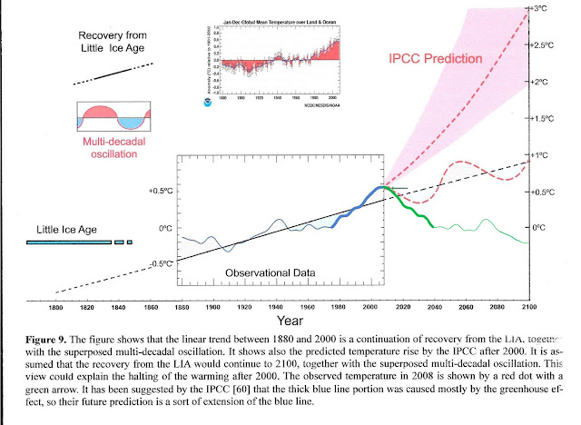
See Fig 1 at
http://climatesense-norpag.blogspot.com/2016/03/the-imminent-collapse-of-cagw-delusion.html
Fig1 (Amended ( Green Line Added) from Syun-Ichi Akasofu) http://www.scirp.org/journal/PaperInformation.aspx?paperID=3217
Figure 1 above compares the IPCC forecast with the Akasofu paper forecast and with the simple but most economic working hypothesis of this post (green line) that the peak at about 2003 is the most recent peak in the millennial cycle so obvious in the temperature data.The data also shows that the well documented 60 year temperature cycle coincidentally peaks at about the same time.
The temperature projections of the IPCC – UK Met office models and all the impact studies which derive from them have no solid foundation in empirical science being derived from inherently useless and specifically structurally flawed models. They provide no basis for the discussion of future climate trends and represent an enormous waste of time and money. As a foundation for Governmental climate and energy policy their forecasts are already seen to be grossly in error and are therefore worse than useless.
A new forecasting paradigm needs to be adopted.
Here are the latest forecasts and conclusions
“3.Forecasts
3.1 Long Term .
I am a firm believer in the value of Ockham’s razor thus the simplest working hypothesis based on the weight of all the data is that the millennial temperature cycle peaked at about 2003 and that the general trends from 990 – 2003 seen in Fig 4 will repeat from 2003-3016 with the depths of the next LIA at about 2640.
3.2 Medium Term.
Looking at the shorter 60+/- year wavelengths the simplest hypothesis is that the cooling trend from 2003 forward will simply be a mirror image of the rising trend. This is illustrated by the green curve in Fig,1.which shows cooling until 2038 ,slight warming to 2073, then cooling to the end of the century.
3.3 Current Trends
The cooling trend from the millennial peak at 2003 is illustrated in blue in Fig 5. From 2015 on,the decadal cooling trend is obscured by the current El Nino. The El Nino peaked in March 2016. Thereafter during 2017 – 2019 we might reasonably expect a cooling at least as great as that seen during the 1998 El Nino decline in Fig 5 – about 0.9 C
It is worth noting that the increase in the neutron count in 2007 seen in Fig 8 indicated a possible solar regime change which might produce an unexpectedly sharp decline in RSS temperatures 12 years later – 2019 +/- to levels significantly below the blue trend line in Fig 5.
4.Conclusions.
To the detriment of the reputation of science in general, establishment climate scientists made two egregious errors of judgment in their method of approach to climate forecasting and thus in their advice to policy makers in successive SPMs. First, they based their analyses on inherently untestable and specifically structurally flawed models which included many questionable assumptions. Second they totally ignored the natural, solar driven , millennial and multi-decadal quasi-cycles. Unless we know where we are with regard to and then incorporate the phase of the millennial cycle in particular, useful forecasting is simply impossible.
It is fashionable in establishment climate circles to present climate forecasting as a “wicked” problem.I would by contrast contend that by adopting the appropriate time scale and method for analysis it becomes entirely tractable so that commonsense working hypotheses with sufficient likely accuracy and chances of success to guide policy can be formulated.
If the real outcomes follow the near term forecasts in para 3.3 above I suggest that the establishment position is untenable past 2020.This is imminent in climate terms. The essential point of this post is that the 2003 peak in Fig 1 marks a millennial peak which is totally ignored in all the IPCC projections.”
PS For Leif – I’m sure that you regard all the above as idle speculation. From my viewpoint your approach is that of someone looking at a large pointilist painting from about 6 inches away.
Better than to look at from a mile away.
I was waiting for the last of the usual suspects to show up and peddle their pseudo-science. You did not disappoint.
about your ‘idle speculation’ as you call it, I’ll say with Tweedledee:
‘if it was so, it might be; and if it were so, it would be; but as it isn’t, it ain’t’
In fact, the pink IPCC projection looks like a much better fit to the blue curve than Akasofu’s green curve.
Dr Norman Page April 22, 2016 at 9:30 am Edit
Oh, sure, forecasting the future evolution of one of the more complex systems on the planet is “straightforward” and can be done with “reasonably useful accuracy” … riiiiiight … the mere fact that nobody has EVER been able to forecast the future climate it doesn’t stop the good Doctor.
Like the man said, if you’re so smart, why ain’t you rich? Anyone who could actually “forecast the future climate trends with likely reasonably useful accuracy” like you claim you can do would be able to make millions off it, farmers and city planners and hedge fund managers would be sitting at your feet waiting for the words of wisdom …
w.
Somehow it strikes me that goes for all the other ones who who peddle their wisdom…
Willis .
A review of candidate proxy data reconstructions and the historical record of climate during the last 2000 years suggests that, at this time, the most useful reconstruction for identifying N H temperature trends in the latest important millennial cycle may be that of Christiansen and Ljungqvist 2012 (Fig 5) Fig 9 here: http://www.clim-past.net/8/765/2012/cp-8-765-2012.pdf
The principal components of climate change of interest on human time scales are embraced in the millennial and 60 year cycles . The amplitude of the former is about 1.8 and the latter about 0.3.See Figs 9 and 15 at http://climatesense-norpag.blogspot.com/2014/07/climate-forecasting-methods-and-cooling.html
http://2.bp.blogspot.com/-4nY2wr6L-WY/U81v9OzFkfI/AAAAAAAAATM/NA6lV86_Mx4/s1600/fig5.jpg
The amplitude of the millennial cycle is taken from the 50 year moving average. The cycle is asymmetric with a downslope of about 650 years or on average 0.0028/year. Also note the amplitude of the variability about the moving average.
Here is what I say re our ability to “prove” future trends. See
http://climatesense-norpag.blogspot.com/2015/08/the-epistemology-of-climate-forecasting.html
“Ava asks – the blue line is almost flat. – When will we know for sure that we are on the down slope of the thousand year cycle and heading towards another Little Ice Age.
Grandpa says- I’m glad to see that you have developed an early interest in Epistemology. Remember ,I mentioned the 60 year cycle, well, the data shows that the temperature peak in 2003 was close to a peak in both that cycle and the 1000 year cycle. If we are now entering the downslope of the 1000 year cycle then the next peak in the 60 year cycle at about 2063 should be lower than the 2003 peak and the next 60 year peak after that at about 2123 should be lower again, so, by that time ,if the peak is lower, we will be pretty sure that we are on our way to the next little ice age.
That is a long time to wait, but we will get some useful clues a long time before that. Look again at the red curve in Fig 3 – you can see that from the beginning of 2007 to the end of 2009 solar activity dropped to the lowest it has been for a long time. Remember the 12 year delay between the 1991 solar activity peak and the 2003 temperature trend break. , if there is a similar delay in the response to lower solar activity , earth should see a cold spell from 2019 to 2021 when you will be in Middle School.
It should also be noticeably cooler at the coolest part of the 60 year cycle – halfway through the present 60 year cycle at about 2033.
We can watch for these things to happen but meanwhile keep in mind that the overall cyclic trends can be disturbed for a time in some years by the El Nino weather patterns in the Pacific and the associated high temperatures that we see in for example 1998 ,2010 and especially from 2015 on.
Fig 4”
Willis this is the nature of the beast and about as good as we can do. The main take away is the if my 2020 forecast is in the ball park the establishment forecast must of necessity surely be seen as in need of serious re-assessment.
Here is the reason I’m not rich.
“In the Novum Organum (the new instrumentality for the acquisition of knowledge) Francis Bacon classified the intellectual fallacies of his time under four headings which he called idols. The fourth of these were described as :
Idols of the Theater are those which are due to sophistry and false learning. These idols are built up in the field of theology, philosophy, and science, and because they are defended by learned groups are accepted without question by the masses. When false philosophies have been cultivated and have attained a wide sphere of dominion in the world of the intellect they are no longer questioned. False superstructures are raised on false foundations, and in the end systems barren of merit parade their grandeur on the stage of the world.”
Climate science has fallen victim to this fourth type of idol.
http://www.sirbacon.org/links/4idols.
Dr Norman Page April 22, 2016 at 12:44 pm
Dr. Page, since Christiansen and Ljunqvist never archived either their code or their data, I fear that their “study” is nothing but useless anecdote—pretty-appearing anecdote, perhaps even impressive anecdote, but anecdote nonetheless.
Anyone using it is either clueless about the study, or is knowingly using anecdotal unverifiable claims … which category are you in?
w.
Willis. Reading the details of the Christiansen paper methods persuades me that it gives a usable representation of reality’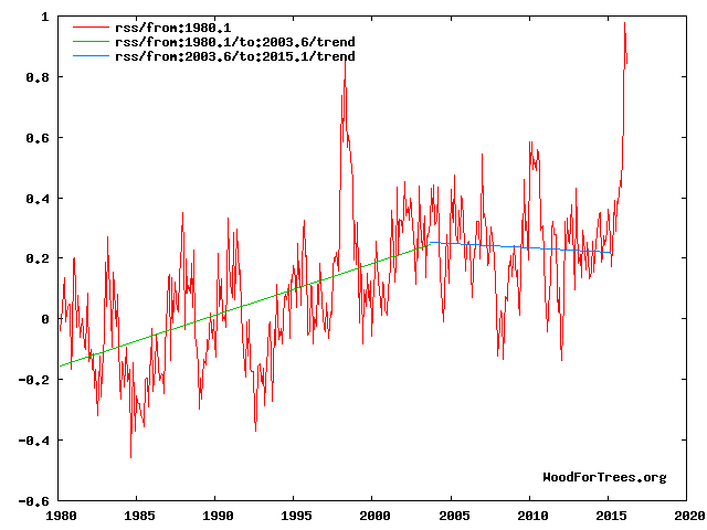
The essential point of the post is that the 2003 peak in Fig 1 marks a millennial peak which is totally ignored in all the IPCC projections.”
Here is a close up look
The El Nino peaks are temporary aberrations which can be ignored when analyzing trends.
No doubt the coincidence of the millennial peak at 2003+/- with the peaks in Evaporative Cooling and Temperature in Figs 5 and 6 at
htps://wattsupwiththat.com/2015/11/11/tropical-evaporative-cooling/
are entirely accidental unless some genius could think up a mechanism.
Link should be https://wattsupwiththat.com/2015/11/11/tropical-evaporative-cooling/
lsvalgaard April 22, 2016 at 10:25 am
Hmmm, not much unlike this event:
I quoted to someone the CAGW theory that one molecule of CO2 warms up by whole 1C each of the neighbouring 2,500 molecules of air and still stays at the same temperature,, in response he threw the same ‘fool me’ quote back at me.
How apt.
I suspect that your assertion that the every 100 extra CO2 ppm would account for 0.5C of warming would fall into same category.
every 100 extra CO2 ppm would account for 0.5C of warming would fall into same category
As you always say: I just follow the data, and that is what they show. Right or wrong? You decide for yourself based on your own bias.
But you are silent about the change of explanation for your idea about LOD. Prudent of you.
As I said you invented that, and asked you to find a quote, or admit you told a ‘porky’, you dismally failed.
What I wrote in 2014 is here
https://hal.archives-ouvertes.fr/hal-01071375v2/document
see page 3
Discussion
…….
“At the current state of knowledge, the most realistic alternative is the indirect solar effect, whereby a possible mechanism could be postulated along line:
Solar activity – ocean & atmospheric temperatures – oceanic and atmospheric circulation – angular momentum exchange – Earth’s rate of rotation (LOD) – secular change in perceived geomagnetic field.”
This is what I wrote few minutes ago:
Despite all the obfuscations the most likely scenario is:
”Solar activity has an effect on ocean & atmospheric temperatures and circulation which in turn via the angular momentum exchange affects the Earth’s rate of rotation (LOD).”
https://wattsupwiththat.com/2016/04/20/ceemd-and-sunspots/comment-page-1/#comment-2196753
you told a ‘porky’ you can’t find a quote to support it.
Considering your age and your past achievements in advancing solar science, I am happy to let you get away with it.
Over to you, let’s have another laugh.
Already in 2014 you had changed your explanation. Look back through earlier posts on WUWT [or elsewhere if applicable] and you’ll surely find where you where pushing the penetration of the solar field to the core and my debunking of it. Where would you otherwise find “that none of the solar magnetic energy can penetrate deep enough to alter the core’s angular momentum (CAM)”. So, go look, don’t be shy, and try to be honest.
No doc you got it wrong, I never claimed what you say.
You confusing two totally different things. I wrote or claimed number of times existence of a possible link between earthquakes and geomagnetic storms, due to telluric currents induction in the lithosphere affecting weak tectonic junctures
http://www.vukcevic.talktalk.net/TF.jpg
I am happy to let you off on this one, even you can make a mistake.
But I’ll not let you off. Honesty has never been a strong side of your nature. My objection that you referred to was specifically directed at your claim in the past that the solar field penetrated into the core. I don’t think you could have come up with that objection on your own. It is OK for you to change your mind [especially away from your ludicrous first idea], but it is not OK to be dishonest about it and hoping I would not notice.
Dr. Svalgaard
Insults I do not do.
Find a quote and come back.
Fair enough in anyone’s book.
Telling you how it is should not be construed as an insult. If you are interested find the quote yourself. You are better positioned to do that, and I have other things to do.
vukcevic: “I suspect that your assertion that the every 100 extra CO2 ppm would account for 0.5C of warming would fall into same category.”
Dr. Svalgaard: “As you always say: I just follow the data, and that is what they show. Right or wrong? You decide for yourself based on your own bias.”
I am truly flattered that on this most contention of the issues you Dr. Svalgaard of the Stanford University (the most famous solar scientist in the world, since slip-up of the NASA’s Dr Hathaway) decided to take Vuk’s scientific approach.
It is worth a terrific laugh on any day, at any time and at any price !
Now lets take look at this new scientific ‘I just follow the data, and that is what they show’ tenet:
In this graph
http://www.vukcevic.talktalk.net/GT-GMF1.gif
it can be clearly seen that temperature rose by 0.5C (Svalgaard theory: caused by rise of 100ppm in CO2) is equivalent to fall of the global magnetic field of about 3.5 microTesla.
I leave to readers if by following the Dr. Svalgaard’s CO2 theory, they would agree that rise of 100ppm in the CO2 concentration has caused the fall of 3.5 microTesla in the Earth’s magnetic field. No doubt that most od Dr.S’s ‘groupies’ would instantly agree.
Now, if that is case, I can only say:
‘things are far worse than expected’.
caused by rise of 100ppm in CO2) is equivalent to fall of the global magnetic field of about 3.5 microTesla.
Only on the goofy and wrong notion that the geomagnetic field has anything to do with the global temeporature. The 0.5 degree is what Lean et al. found here Figure 2 of http://www.leif.org/EOS/123222295-Lean-Trends.pdf
If you don’t like it, take it up with her. That is what the data shows. Like it or not.
Hey, hey, let’s get this right.
It was rise in the mighty CO2 molecule from 280 to 400ppm, that caused fall in the Earth’s magnetic field, not the tiny temperature rise from 287.5 to 288 degree K.
‘things are far, far worse than expected’
It was rise in the mighty CO2 molecule from 280 to 400ppm, that caused fall in the Earth’s magnetic field
In true style you continue to spout nonsense.
“The 0.5 degree is what Lean et al. If you don’t like it, take it up with her. That is what the data shows. Like it or not.”
No chance, I am not in a habit of having a laugh on account of any woman (call it sexist if you wish) and especially not at a particularly nice lady as Ms Judith Lean is.
No chance, I am not in a habit of having a laugh on account of any woman
Try science instead of acting as a laughing clown. Judith would know the difference.
I happened quite randomly upon this very recent and interesting paper today that adds support to my solar thesis:
Relationships between solar activity and variations in SST and atmospheric circulation in the stratosphere and troposphere
“Correlation coefficients between annual sunspot numbers and monthly SST from 1901 to 2011 were calculated, and the areas where the r-values were equal or greater than the 95% significance level (<0.05) were plotted ( Fig. 1). To determine the influence of solar variability on weather conditions during the solar maximum phase, we selected three periods (9 years in total) when solar activity was at a maximum during the period from 1979 to 2011: 1979–1981, 1989–1991 and 2000–2002."
http://ars.els-cdn.com/content/image/1-s2.0-S104061821501143X-gr1.jpg
that adds support to my solar thesis
What a terrible paper. Here are their data:
http://www.leif.org/research/Terrible-Paper-Fig-2.png
The R^2 is 0.04.
The authors mention several peaks occurring in the second year after the sunspot number maximum, which is completely understandable given that in almost all cases the TSI peaked after the SSN peaked by about a year, which is one point I’ve been hammering home on this post:
SC21, the SSN peak was in 1979, then 1980; the TSI peak was in 1980, followed by 1981
SC22, the SSN peak was in 1991, 1990 was second; the TSI rank was 1990,1991,1992
SC23, the SSN rank was in 2000, 2001, 2002; the TSI rank was 2002, 2000, 2001
SC24, the SSN peak was in 2014; the TSI peak was in 2015
“Furthermore, the analysis period included the strong El Niño event in 1982 and the eruption of Mt. Pinatubo in 1991. The results obtained did not show any significant differences when these events were excluded from the analysis.”
Remember the solar max NE Pacific “Blob” that is no longer there?
Fig 8
http://www.sciencedirect.com/science?_ob=MiamiCaptionURL&_method=retrieve&_eid=1-s2.0-S104061821501143X&_image=1-s2.0-S104061821501143X-gr8.jpg&_cid=271860&_explode=defaultEXP_LIST&_idxType=defaultREF_WORK_INDEX_TYPE&_alpha=defaultALPHA&_ba=&_rdoc=1&_fmt=FULL&_issn=10406182&_pii=S104061821501143X&md5=422ce977a0bc2c18537ef37bce1d5c6c
Remember the heavy rains wind hail and tornadoes in the US right in the darkest purple area on this image, in the mid-south, last November/December, the second year after the SSN solar max?
Fig 10
http://www.sciencedirect.com/science?_ob=MiamiCaptionURL&_method=retrieve&_eid=1-s2.0-S104061821501143X&_image=1-s2.0-S104061821501143X-gr10.jpg&_cid=271860&_explode=defaultEXP_LIST&_idxType=defaultREF_WORK_INDEX_TYPE&_alpha=defaultALPHA&_ba=&_rdoc=1&_fmt=FULL&_issn=10406182&_pii=S104061821501143X&md5=6d1f6937231b7bf05b0e1910c6b58970
SC24, the SSN peak was in 2014; the TSI peak was in 2015
The paper stops in 2011….
The TSI normally follows SSN. 2014-2015 are anomalous:
http://www.leif.org/research/Non-Conforming-SC24.pdf
It doesn’t matter if their paper stops at 2011, as my point stands anyway, as I just used the most recent cycle data too to demonstrate exactly what you said here “The TSI normally follows SSN.”
However, this part is a puzzle: “2014-2015 are anomalous” in the sense of TSI and SSN?
How can that be if The TSI normally follows SSN?
After all v2 SSN was 113.3 in 2014, 69.8 in 2015, and SORCE TSI was higher in 2015 than 2014!
How does it follow then that they are anomalous in that sense that you have defined? In that sense it seems like a normal cycle. The TSI peak followed the SSN peak, just as I have been saying.
I’ll look at your paper in the morning. Thanks.
Bob, I think Leif meant “follows” in the sense of “is in step with”, and not in the sense of “comes after”. It’s the only way his statement makes sense.
w.
yes, ‘in step with’, not ‘with delay’.
Bob Weber April 22, 2016 at 8:56 pm
Thanks, Bob, but that paper is a joke. For example, they say:
It appears they never heard of the Bonferroni correction. Have you heard of it? If not, you definitely should look it up … and they absolutely should look it up. Basically, if you look at tiny subsections of any data, like say “at 38°N 126°W in December” you’ll find so-call “significant” results all the time which are not significant at all.
They also have made no attempt to correct for autocorrelation, which is a huge issue in natural datasets. Finally, for strongly cyclical type signals like sunspots, you need to buttress your statistical calculations with Monte Carlo analysis or you’ll get fooled by spurious correlations.
As they have done none of these required steps, they have converted what could have been an interesting study into garbage. You cannot trust a single one of their claims of significance, they are meaningless.
Regards,
w.
I fully agree, the paper is junk.
Thanks for your input. Maybe you’re right but I’d really have look a lot closer to make that kind of call.
The authors made a few good points that resonated with my observations, as I pointed out. Dr. Jeff Johnstone had a paper last year about the SLP/SSTs in the NE Pacific that matched the characteristics of the description in this paper about that area, and timing of such, and my observations of the timing of last year’s NE pacific blob. So while you pan the paper, I do think there’s a some nuggets of gold in there. I’m sure the subject will be returned to repeatedly by others with other methods.
Now, back to the time rate of TSI change thing…. that’s what I think you really need to see. Energy. Focus on the time rate of energy into the system too, not just statistics! The absolute TSI at solar minimums going into the cycle looks too small etc, right? If you’ll just take the time and run those annual PMOD rate of annual TSI change numbers, it’s only 39 years – and plot them against SST, then you’ll finally really learn something unforgettably great about how sensitive SSTs are to changing TSI.
Bob Weber April 22, 2016 at 5:32 pm
Bob, I have never seen any evidence that “TSI lags sunspot numbers”. So I just went and looked at the monthly TSI (ARIM) and sunspot data. I didn’t find any lag. Next, I looked at the monthly TSI (PMOD) and sunspot data … same result, no lag.
Next, I looked at the R^2 and the p-values. For annual data, they are 0.89 (p-value less than 2E-16) for the PMOD values, and 0.67 for the ACRIM values.
So no, the use of sunspots in place of TSI data is not misleading in any sense. Particularly for the PMOD data it is very close to the sunspot data.
Regards,
w.
Willis check in my comment just above for the timing of each cycle TSI peak vs SSN peak – TSI peaks about one year after SSN peak, most of the time, using annual data. It matters. I just scattered PMOD monthly with v2 SSN monthly and got an R^2 of 0.5872. The plot is wide in all directions and I’d be very concerned about basing all my conclusions on monthly data, as most of the data is far off the line.
Double checking now on daily data: R^2 of 0.2732 – it’s worse. Daily TSI is better than daily SSN.
Using annual data: R^2 of 0.8582, close to yours.
In case you missed it, here’s a prior comment I left you about why daily TSI data is more meaningful to understanding the ongoing and ever-changing solar influence, and how it can vary 4-5X more than “0.1%”.
So your conclusion here is wrong, in a qualified sense: “So no, the use of sunspots in place of TSI data is not misleading in any sense. Particularly for the PMOD data it is very close to the sunspot data.”
It is misleading in the sense that after 1978 there is no purpose in using sunspot numbers as there is PMOD and SORCE TSI, because the timing of changes and magnitudes of TSI is vitally important to each part of the SST/OHC continuium, as I’ve tried to explain.
If you use only sunspot numbers you’ll be off in your timing and magnitude in evaluating what the solar activity is doing to the earth, unless you take into account the approximently one year lag, which could easily throw off an ENSO-solar evaluation if not understood.
There’s a couple other very important rules of the road you need to know about but it’s late. It’s been fun.
It is misleading in the sense that after 1978 there is no purpose in using sunspot numbers as there is PMOD
The errors in TSI PMod are larger than in the SSN.
Except for SC24, TSI can be calculated from the SSN with no lag:
http://www.leif.org/research/TSI-from-SSN-Froehlich,png
see: http://www.leif.org/EOS/TSI-Uncertainties-Froehlich.pdf
http://www.leif.org/research/TSI-from-SSN-Froehlich.png
WP plays tricks again.
http://www.leif.org/research/TSI-From-SSN-Froehlich2.png
That’s really nice but with so many choices for a TSI-SSN curve to use, it’s more like choosing which warmist climate model you think represents reality. How would you know if any does?
Here’s PMOD 2013 monthly data compared to v2 SSN, can you tell me what’s wrong with this picture Leif?
1361.0946 96.1
1361.2148 60.9
1361.2595 78.3
1361.1320 107.3
1361.3467 120.2
1361.3474 76.7
1361.3554 86.2
1361.3771 91.8
1361.4095 54.5
1361.0501 114.4
1361.0169 113.9
1361.2839 124.2
TSI CANNOT be directly computed from SSN! Forget about it. The relationship is all over the place.
Claus Froehlich [who makes PMOD] disagrees with you:
TSI = base + 0.27202E-1 SSN^0.5 + 0.61564E-2 SSN – 0.12968E-3 SSN^1.5
OK, it’s 3am where I am, but I’ll stay up a while longer for this one ’cause it’s worth it. I’ll show that I’m right – and I don’t even know that yet for sure!!
I will enter your friend’s formula into a sheet, enter the monthly SSNs I used above just for 2013 as an example, then I will compute the result of the formula, compute a difference from actual and a % error for each month, and total annual error. If that error is greater than 5% in any month, the model is junk.
The differences between actual and modeled months are shown below with the formula base set to 1360.359 so the difference is zero in the first month. The % error is the difference divided by the total variation, ie, the range of the 12 months, the max-min range, 0.393.
diff % error
0.331 84%
0.268 68%
-0.025 -6%
0.121 31%
0.366 93%
0.317 81%
0.307 78%
0.567 144%
-0.145 -37%
-0.176 -45%
0.037 9%
1361.410
1361.017
0.393
I don’t know about you Dr. Svalgaard, but I wouldn’t call the demonstrated actual model error range of -45 to 144% “good” or acceptable. An error of 0.567 in one month is completely unacceptable for TSI. The maximum three month swing in error is 0.567-(-0.176)=0.743 just for this one year’s monthly data!
Maybe annual data might work better, but if the error is so great at monthly time scales you’ll lose too much resolution on TSI, making this model useless for understanding how TSI really changes throughout a year if you’re using monthly sunspot numbers as your base. Sorry. It’s too bad too. It all looked so promising.
You did not heed my warning that SC24 is anomalous
http://www.leif.org/research/Non-Conforming-SC24.pdf
read it.
Bob Weber April 22, 2016 at 10:49 pm Edit
Bob, you don’t understand. I just checked both the PMOD and the ACRIM data. Neither one shows a one-year lag. And Leif says the same, just above.
Since you have not given us the sources of your PMOD data, I fear I’ll believe my own figures that there is no “one-year lag” until you give us the links.
w.
Willis,
SC24 is anomalous:
http://www.leif.org/research/Non-Conforming-SC24.pdf
At this point we don’t know why, except that it is not instrumental error.
“Since you have not given us the sources of your PMOD data, I fear I’ll believe my own figures that there is no “one-year lag” until you give us the links.” That is just a lie, easily disproven!!!
I don’t have to check that again Willis, and I never hid any data from you either, as I posted this link at 9:45am for PMOD, over 13 hours ago – if you paid any real attention to what I say you’d know that – here it is again – nothing up my sleeve – ftp://ftp.pmodwrc.ch/pub/data/irradiance/composite/DataPlots/composite_42_65_1602.dat.
I also showed each instance of the TSI peak lag(s) here after the cycle SSN peaks:
SC21, the SSN peak was in 1979, then 1980; the TSI peak was in 1980, followed by 1981
SC22, the SSN peak was in 1991, 1990 was second; the TSI rank was 1990,1991,1992
SC23, the SSN rank was in 2000, 2001, 2002; the TSI rank was 2002, 2000, 2001
SC24, the SSN peak was in 2014; the TSI peak was in 2015
A one year lag occurs about 75-80% of the time.
Year PMOD TSI F10.7 v2SSN
2002 1361.7132 179.5 163.6
2000 1361.7102 179.4 173.9
1980 1361.6522 198.6 218.9
1981 1361.6424 202.6 198.9
2001 1361.6349 181.3 170.4
1989 1361.6224 213.5 211.1
1979 1361.5670 191.9 220.1
1990 1361.5669 189.8 191.8
1991 1361.4917 208.1 203.3
1999 1361.4889 154.1 136.3
1992 1361.3106 150.5 133.0
1983 1361.3050 119.6 91.0
1982 1361.2916 175.1 162.4
2015 1361.2647 117.6 69.8
2003 1361.2381 128.7 99.3
1998 1361.2250 118.1 88.3
2013 1361.2142 122.8 94.0
2012 1361.1778 119.9 84.5
2014 1361.1654 146.1 113.3
1988 1361.1209 141.0 123.0
2016 1361.0771 106.4
2011 1361.0529 113.4 80.8
1978 1361.0445 164.3 131.0
2004 1361.0075 106.4 65.3
1993 1361.0014 109.7 76.1
1984 1360.8737 100.9 60.5
1997 1360.8582 81.0 28.9
1994 1360.8361 85.8 44.9
2005 1360.8343 91.7 45.8
1987 1360.8100 85.3 33.9
2010 1360.8086 80.0 24.9
1995 1360.7475 77.2 25.1
1986 1360.7273 74.0 14.8
2006 1360.7247 80.0 24.7
1985 1360.7176 74.7 20.6
1996 1360.6935 72.0 11.6
2007 1360.5934 73.1 12.6
2008 1360.5711 69.0 4.2
2009 1360.5569 70.6 4.8
Nothing was hidden from you Willis. Back again to accusing people of withholding data eh?
Here we have Leif again “Except for SC24, TSI can be calculated from the SSN with no lag: BS!!
What is the matter with you guys? The annual TSI lags are right in the table above in plain sight. Take your blinders off.
Secondly I didn’t say SC24 wasn’t anomalous, I just said Leif’s criteria for that as first stated here today wasn’t met. The SC24 TSI peak did lag the SSN peak by one year, using annual data, so what was so anomalous about that, given his stated criteria?
http://www.sidc.be/silso/DATA/SN_d_tot_V2.0.txt
http://www.sidc.be/silso/DATA/SN_m_tot_V2.0.txt
http://www.sidc.be/silso/DATA/SN_y_tot_V2.0.txt
ftp://ftp.geolab.nrcan.gc.ca/data/solar_flux/monthly_averages/solflux_monthly_average.txt
SC24 is anomalous, and the relationship between TSI and SSN has changed.
Plotting your data list gets us:
http://www.leif.org/research/TSI-Dont-Lag.png
Each curve has its own small variations as shown in the top panel.
If TSI would be lagged 1 year, then shifting it 1 year earlier should improve the agreement between the curves, and it clearly does not. It makes it worse. Thus: no 1 year lag.
But also note the anomalous SC24.
Dr. Svalggard
You make false accusation without able to provide a proof. If you did that in your home state you would end up in a courthouse.
Now you make even more ridiculous request, that I should find evidence that I written what I didn’t write to prove your false accusation.
lsvalgaard April 22, 2016 at 3:11 pm
“If you are interested find the quote yourself. You are better positioned to do that, and I have other things to do.”
In view of the latest exchanges:
I was inclined to accept your work on the new ‘sunspot data’ as probably OK, despite huge alterations ranging from -20% to +30%, in order to eliminate all but the most severe solar variability (even questioning the existence of the Maunder Minimum).
Now you come up with: 100ppm rise in the CO2 is responsible for 0.5C rise in the global temperatures, that is what the data shows. Like it or not.
No, you don’t fool me any longer, sir.
The nice lady Judith Lean came up that figure based on the data available. Complain to her.
And keep looking for your solar penetration idea. It is there.
There is another nice lady called Judith (Curry), this time a professional climate scientist.
Your quote would have far more credibility if you quote on the climate matters a renown climate than a solar scientist.
Anyone can rattle false accusations, people loose their respect for those who do it but can’t prove it.
a professional climate scientist.
All the sudden climate scientists are doing valid science? that is a new one. Curry may be a special case, why don’t you ask her what she thinks the 100 ppm would do. Now, Lean is a recognized climate expert:
http://www.nrl.navy.mil/media/news-releases/2014/dr-judith-lean-receives-double-honors-in-geophysical-research-letters-top-40
Nobody is fishing for respect, perhaps with the exception of you.
“Nobody is fishing for respect, perhaps with the exception of you.”
Respect is not attained by a hobby of poking fun at the ‘settle science’, none asked for, none gained.
However your respect is a great danger by continuously rattling a false accusation that you can prove, it borders on bizarre, next time I see it, I’ll probably burst into laughter.
On matter of two Judiths :
I don’t entirely agree with Dr. Curry on number of matters, but respect her views.
Your favourite Judith, the one you like to quote, in the paper you are quoting with your newly acquired admiration for the CAGW (or was it always there, but kept under the blanket) she is promoting ‘Modern Solar Maximum’
http://www.leif.org/EOS/123222295-Lean-Trends.pdf
see fig 5.
Am I to take it that you abandon your most recent insistence that there is no such thing as ‘ Modern Maximum’ ? or are you just taking her view on the CO2 – AGW stand, but reject her view on the solar stuff?
Lean’s paper was written six years ago, before it was shown that there is no Grand Modern Maximum. Your attempt to drag this in as relevant is pathetic.
Lean’s figure for the 100 ppm effect is based on her analysis of the data. Not my number. When people ask me what the effect would be, I check the literature in order to give a number backed up by valid analysis without my bias. To call that CAGW is also pathetic and ad-hom. Especially the ‘C’ in CAGW. Let me tell you that global warming [whatever the reason] is GOOD. Warm is much better than cold. In a hundred years we will have adapted to whatever happens, as we have always done, so no ‘C’.
Lastly, if my recollection is good, your argument used to be that the Earth’s main field which originates in the Earth’s molten core varied long-term in sync with solar activity and you quoted Dickey [presumably agreeing with her] for suggesting that some solar process [solar activity caused by its magnetic field] could affect the core. It seems that you have gotten cold feet on that idea, which is good, because it is wrong.
typo correction https://wattsupwiththat.com/2016/04/20/ceemd-and-sunspots/comment-page-1/#comment-2197626
Come on now, getting all touchy, not the self promoting Donald Trump’s trait you are modelling yourself on.
‘Ad home’ is not your numerous dispersions on my character you freely throw about so freely, but most of time I ignore since they are not true.
An now this super-sensitive California desert cactus blossom
is complaining that calling 100ppm CO2 as cause of 0.5C rise in CO2, AGW is a terrible insult.
That means that at least half or more of the global temperature rise is due to the CO2; no one outside AGW thinks or believes that.
What Dickey from NASA-JPL writes it’s her views not mine, but if you read it you will see you misquoted her.
Yes, the warming is and was good, it was caused most likely by the Solar Modern Grand Maximum, you think you may have obliterated out of existence for ever. Don’t be too sure, when the likely cooling sets in, it may take 20-30 years, people and science will reject all these fancy so called theories.
CO2 could rise to 500ppm but the temperatures may stay still or even fall.
As far as I can see it both the ‘Svalggard SSN’ and 0.xx C/100CO2ppm will be rejected as follies of the early years of XXI century.
What Dickey from NASA-JPL writes it’s her views not mine
Ha, you used to quite her extensively and take her words as support for your ideas, but it is progress that you have stopped doing that. But at least you now know when you were promoting her solar influence on the Earth’s core.
Global warming is the result probably of several causes. different people have different opinions on how to apportion the total changes to which causes. Lean’s assessment does a pretty good job, actually better than most. Is she correct? only time will tell. My [balanced] opinion you can find here http://www.leif.org/research/Climate-Change-My-View.pdf
As IPCC [AR5] says: “No best estimate for equilibrium climate sensitivity can now be given because of a lack of agreement on values across assessed lines of evidence and studies”.
What does seem rather definite is that your ideas are wanting and are not a fruitful road to take [junk science never is].
Dr Svalgaard:
isn’t the relationship between temperature and changes in CO2 levels logarithmic?
Thus, the increase in CO2 levels from 280ppm to 380 ppm will not have the same effect as the increase from 380 to 480 ppm.
The question:
“what is the effect on temperature of a 100ppm increase in CO2 levels?” really cant be answered, unless one specifies the level of CO2 in the atmosphere before (or after) the increase.
Yeah, but Lean’s number is based on current conditions because it is based on data up to the present.
“Ha, you used to quite her extensively and take her words as support for your ideas, but it is progress that you have stopped doing that.”
Are you now accusing Dickey the NASA-JPL’s top expert on the geo-dynamics saying that the sun ‘runs’ processes in the Earth core, as I said your comments are getting more bizarre by the minute, certainly worth a good laugh.
As for my writing, quote my words, not your wavering imagination and fading memory.
So J.Lean is in your view correct about AGW, but absolutely wrong about the Modern Solar Maximum, in the same paper on the same page.
Bizarre Plurimus ! ! .
Are you now accusing Dickey the NASA-JPL’s top expert on the geo-dynamics saying that the sun ‘runs’ processes in the Earth core
Actually I only have your words for that: Vuk quoting Dickey: “an external (e.g. solar) process affects the core”. Perhaps you just made that up and she never said it, but at least you claim that she did.
So J.Lean is in your view correct about AGW, but absolutely wrong about the Modern Solar Maximum, in the same paper on the same page.
Correct. The paper was written in 2010 long before we knew that the Modern maximum was not Grand. Lean cannot be faulted for not being clairvoyant.
Your attempts of deflecting attention from your failures fall flat. Time for you to call it quits.
You do write lot of nonsense. The quote is:
“One possibility is the movements of Earth’s core (where Earth’s magnetic field originates) might disturb Earth’s magnetic shielding of charged-particle (i.e., cosmic ray) fluxes that have been hypothesized to affect the formation of clouds. This could affect how much of the sun’s energy is reflected back to space and how much is absorbed by our planet. Other possibilities are that some other core process could be having a more indirect effect on climate, or that an external (e.g. solar) process affects the core and climate simultaneously.”, her words not mine.
NASA Study Goes to Earth’s Core for Climate Insights
http://www.nasa.gov/topics/earth/features/earth20110309.html
Only a dummy would interpret that as the solar magnetic field is penetrating the core, it is most likely that she thinks it is solar movement around its bary centre, and that is probably is a no-no at JPL.
If that is the best you can come up with justifying your ‘porky’ that I wrote that solar magnetic field penetrates earth core it is THE MOST PATHETIC STATEMENT that could come from scientist of your stature. No apologies required.
ps. prompted by your newly acquired AGW conversion, here is the only page in my new science book just published on line
http://www.vukcevic.talktalk.net/CAGW.gif
I’m sure you might wish to comment
As I said “an external (e.g. solar) process affects the core”.
But you go on further flights of fancy, e.g. in this one:
http://www.leif.org/research/Vuk-Failure-39.png
where you compare Lean’s TSI with changes in the Earth’s main field [stemming from the core] and suggest that 0.45 W/m2 causes (?) a decrease of the main field of 0.75 microTesla [or is it the other way around? it is hard to say with you].
I think that readers [and WUWT] are ill-served with such nonsense.
Thanks for bringing that to the attention of the readers, if there are any left, that is.
It is a great discovery, another confirmation that on the large scale in the long term, both the sun’s and Earth’s magnetic field changes are governed by solar system planetary dynamics.
But your interpretation is a lot nonsense, and then you claim that you have better things to do.
So now you are saying that Global Warming is controlled by the planets perturbing the sun [or is it only the Earth?]. Perhaps you could also make my horoscope to predict my future.
I think this particular topic has reached its well-deserved dead end.
I agree, let’s not discuss it further. It is so dead ended in fact that it’s part of the blog policy to not discuss it anymore as it invariably ends up in food [fights].
huh!, bad typo there:
it should be :However your respect is a great danger by continuously rattling a false accusation that you can’t prove, it borders on bizarre, next time I see it, I’ll probably burst into laughter.”
Who would care?
Willis,
I love how you do your data analysis before checking the literature. However afterwards it is necessary to check what other scientists with quite a lot more effort have found analyzing a lot more than 300 years of data.
I highly recommend the following paper:
McCracken, K. G., et al. “A phenomenological study of the cosmic ray variations over the past 9400 years, and their implications regarding solar activity and the solar dynamo.” Solar Physics 286.2 (2013): 609-627.
The periodicities found in solar modulation of galactic cosmic rays are different whether you analyze the whole data or just the periods without Solar Grand Minima. Specifically the de Vries cycle disappears and reappears following the Halstatt cycle.
http://i1039.photobucket.com/albums/a475/Knownuthing/McCracken%20Fourier_zpspm7dlavb.png
http://i1039.photobucket.com/albums/a475/Knownuthing/McCracken%20Table2_zps29vtxkzn.png
You find traces of the 60, 91 and 113 periodicities as they do when they analyze annual 10Be deposits in the Dye 3 ice core that has a yearly resolution (annual data column) between 1420 and 1992.
The rest of the periodicities you miss because you constrain yourself to such a short period of data. You cannot say much about periodicities longer than about 100 years.
Javier April 23, 2016 at 3:10 pm
Thanks, Javier. If you truly believe that we know the twists and turns that the sun took over the past 9,400 years, then you have not checked “what other scientists with quite a lot more effort have found”. Both the 10Be and the 14C records are fraught with all kinds of problems which we’ve discussed on this site.
Next, as the wavelet analysis above showed, there are dozens of various cycles that pop out of the woodwork, last a hundred years or five hundred years, and then disappear again … and the type of analysis shown above from the paper is totally inadequate for understanding that situation.
http://www.pnas.org/content/109/16/5967/F4.large.jpg
They are ASSUMING that every one of those is a real repeating signal … but we know for a fact that that is not the case. Look at the claimed “De Vries” cycle above. It only exists in a few short periods, and when it does, it’s not a “208 year cycle”, that’s a mockery. Instead, it is a whole host of cycles varying from about 100 years to three hundred years. Sorry, Javier, but your analysis shown above doesn’t even BEGIN to deal with that.
In any case, I’m more than happy to analyze your paper if you will send me a link to the paper and another link to the dataset as used in the study.
Finally, both you and the authors seem entranced with the idea that when you take out part of the data you get different periodicities … for heaven’s sake, what did you expect???
w.
PS—My rule of thumb is that if a claim is only established by a look at proxies from thousands of years ago, it is a very weak claim and should be treated with great suspicion … and your cited paper is no exception. Yes, as you say, you can make all kinds of claims for longer term periodicities … but if you look at the various authors addressing the same question with different proxies, they rarely find the same periodicities.
Willis,
There is no perfect proxy record. Luckily we have two different proxies for the solar modulation of galactic cosmic rays that undergo different climate pathway modification. The knowledge of those pathways has also improved, so our reconstruction of past solar activity combining all this knowledge and both proxies is improving.
You can find the paper:
McCracken, K. G., et al. “A phenomenological study of the cosmic ray variations over the past 9400 years, and their implications regarding solar activity and the solar dynamo.” Solar Physics 286.2 (2013): 609-627.
here:
http://sci-hub.io/10.1007/s11207-013-0265-0
This paper uses different sets of data and some of them are modified by mathematical functions. The data that is available is the main one, that is used to establish the solar modulation function Φ:
“Recent studies (Steinhilber et al., 2012) have combined all available data for the past 9400 years, thereby extracting the solar signal from extraneous atmospheric and climate-related effects. This article examines this new record in both the time and frequency domains, which yields detailed information regarding the time-dependent modulation of the galactic cosmic-rays by the Sun, and by inference, the long-term variability of solar activity and the solar magnetic dynamo.”
This data is available here:
ftp://ftp.ncdc.noaa.gov/pub/data/paleo/climate_forcing/solar_variability/steinhilber2012.txt
ftp://ftp.ncdc.noaa.gov/pub/data/paleo/climate_forcing/solar_variability/steinhilber2012.xls
We can discuss the importance of these periodic oscillations and whether they constitute a true cycle or not, but many of them are found study after study, both in climate proxies and in these solar proxies, so their existence is pretty solid and not due to climate contamination.
@ Willis Eschenbach
April 21, 2016 at 11:14 am : So, a matter of raining on Lief reining in? Sorry, couldn’t resist either.