Guest Post by Bob Tisdale
UPDATE: See the update below Figure 1.24-8 for the IPCC’s correction of their Figure 9.17 from the 5th Assessment Report. Thanks, Nic.
# # #
This post presents model-data comparisons of ocean heat content. It is a correction and update (with 2015 values) of the modeled and observed trends in ocean heat accumulation that were presented in Chapter 1.24 – A Rough Calculation of the Amount of Missing Heat…A Critical Issue of my free ebook On Global Warming and the Illusion of Control – Part 1 (25MB). In that chapter of the book, many of the model trends listed on the graphs were in error, with the trend values too low, bringing them closer to the observations. In other words, my errors favored the models. My apologies for the mistakes. Those errors have been corrected in this post and will be corrected in the ebook in its final release later this year.
# # #
Chapter 1.24 – A Rough Calculation of the Amount of Missing Heat…A Critical Issue
If you’re new to the topic of global warming, you may think discussions of The Missing Heat have to do with the slowdown in global surface warming since the late 1990s, which wasn’t anticipated by climate modeling groups. The term Missing Heat, however, is not related to the slowdown in global surface warming. Missing Heat is used in discussions of the heat being stored in the depths of the oceans.
OVERVIEW

In Chapter 1.10 – Introduction to Radiative Imbalance, I presented the modeled energy imbalance at the top of the atmosphere (TOA). As you’ll recall, there was a very wide spread in the individual model simulations of the top-of-the-atmosphere energy imbalance. (See Figure 1.10-3.) I’ve shortened the timeframe to 1955-2015 in Figure 1.24-1, which is the period for which ocean heat content data are available from the NODC.
NOTE: Following an introduction to the concept of Earth’s energy imbalance, much of Chapter 1.10 – Introduction to Radiative Imbalance is based on the August 2015 post No Consensus: Earth’s Top of Atmosphere Energy Imbalance in CMIP5-Archived (IPCC AR5) Climate Models. [End note.]
Ponder that graph for a moment. The average top-of-the-atmosphere energy imbalance (red curve) in recent years is in the expected range…the range we’ve been told by the climate science community. Example: According to Trenberth et al. (2014) Earth’s Energy Imbalance:
All estimates (OHC and TOA) show that over the past decade the energy imbalance ranges between about 0.5 and 1 Wm-2.
Trenberth et al. (2014) must not have been referring to the individual climate models, because they show a much larger range. In fact, some of the models show relatively high positive TOA energy imbalances, in the neighborhood of +2.5 watts/m^2, while others show negative energy imbalances, roughly -2.5 watts/m^2.
The simulated oceans in the models with the high positive top-of-the-atmosphere energy imbalances have to be accumulating heat at relatively fast rates. On the other hand, the simulated oceans in the models with the negative top-of-the-atmosphere energy imbalances have to be losing heat very quickly. Yes, losing heat.
In this chapter, we’re going to calculate and illustrate the ocean heat accumulation from 1955 to 2015 based on the climate-model-simulated top-of-the-atmosphere energy imbalances for all of the models included in the earlier energy imbalance chapter (Chapter 1.10). We’ll start with the full oceans compared to data for the top 2000 meters, and we’ll then compare models and data for the top 700 meters.
INTRODUCTION
Because the oceans to depth have a tremendous capacity to store heat, they are supposed to be storing about 93% of the excess heat created by the emissions of man-made greenhouse gases. See Figure 1.24-2.

The pie chart in Figure 1.24-2 is based on the Earth’s total energy change inventory from Box 3.1 of Chapter 3 – Observations: Oceans of the IPCC’s 5th Assessment Report. There they write:
Ocean warming dominates the total energy change inventory, accounting for roughly 93% on average from 1971 to 2010 (high confidence). The upper ocean (0-700 m) accounts for about 64% of the total energy change inventory. Melting ice (including Arctic sea ice, ice sheets and glaciers) accounts for 3% of the total, and warming of the continents 3%. Warming of the atmosphere makes up the remaining 1%.
Later in the chapter we’ll address the depths of 0-700 meters.
WE CAN USE THE MODELED ENERGY IMBALANCE AT THE TOP OF THE ATMOSPHERE TO DETERMINE HOW MUCH HEAT THE OCEANS SHOULD BE ACCUMULATING, ACCORDING TO THE MODELS
The ocean heat content outputs of the climate models stored in the Climate Model Intercomparison Project Phase 5 (CMIP5) archive are not available in easy-to-use form at the KNMI Climate Explorer. In fact, I know of no place where ocean heat content outputs are easy to access for any of the CMIP5-based models.
Fortunately, the components of the modeled Energy Imbalance at the Top of the Atmosphere (TOA) are available. So we can determine the energy imbalance, and, in turn, how much heat the oceans should be storing, according to the models. It’s commonly done, as you’ll see.
As you’ll recall from Chapter 1.10 – Introduction to Radiative Imbalance, the energy imbalance at the top of the atmosphere is made up of 3 components (nomenclature and acronym used at the KNMI Climate Explorer are shown in parentheses):
- the amount of sunlight reaching the top of the atmosphere (TOA Incident Shortwave Radiation, rsdt),
- the sunlight being reflected back to space primarily by clouds and volcanic aerosols (TOA Outgoing Shortwave Radiation, rsut), and
- the infrared radiation being emitted by Earth relative to the top of the atmosphere (TOA Outgoing Longwave Radiation, rlut).
The top of the atmosphere energy imbalance is calculated by subtracting the Outgoing Shortwave and Longwave Radiation from Incident Shortwave Radiation.
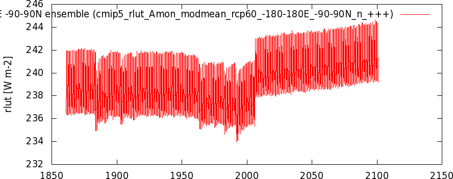
Figure 1.24-3 presents the average top-of-the-atmosphere energy imbalance of the climate models stored in the CMIP5 archive, specifically the multi-model mean of the models using historic and RCP6.0 forcings. We’re discussing the multi-model mean now for simplicity sake…for those new to the topic. The 1955 to 2015 timeframe relates to the NODC’s ocean heat content data for the depths 0-2000 meters (about 6600 feet or about 1.25 miles).

The large dips and rebounds in those model simulations are caused by the aerosols emitted into the stratosphere by explosive volcanic eruptions.
Each year that the top-of-the-atmosphere energy imbalance is positive, the oceans gain heat, and each year the top-of-the-atmosphere energy imbalance is negative, the oceans lose heat. The energy imbalance is positive most of the time, so the modeled oceans should be warming to depth, according to the model mean.
Note: You’ll notice in the title block of Figure 1.24-3 that I excluded three models: one CESM-CAM5 model and two IPSL models. There were shifts at 2006 in the TOA Outgoing Longwave Radiation outputs of all three runs of the CESM-CAM5 model (one with a monstrous shift), which skewed the multi-model mean of that metric for that scenario. (I notified KNMI of that problem, and NCAR has since corrected them. I’ve continued to exclude them so that the models in this chapter are the same in the top-of-the-atmosphere energy imbalance chapter.) I also excluded the two IPSL models because their top-of-the-atmosphere Incident Shortwave Radiation contains a volcanic aerosol component, while all other models do not. (The other models address volcanic aerosols with the Outgoing Shortwave Radiation.)
That leaves 21 models, including BCC-CSM1-1, BCC-CSM1-1-M, CCSM4 (6 runs), CSIRO-MK3-6-0 (10 runs), FIO-ESM (3 runs), GFDL-CM3, GFDL-ESM2G, GISS-E2-H p1, GISS-E2-H p2, GISS-E2-H p3, GISS-E2-R p1, GISS-E2-R p2, GISS-E2-R p3, HadGEM2-AO, HadGEM2-ES (3 runs), MIROC5 (3 runs), MIROC-ESM, MIROC-ESM-CHEM, MRI-CGCM3, NorESM1-M, and NorESM1-ME.
For those models with multiple runs, the ensemble members are averaged before being included in the multi-model mean.
[End note.]
CONVERTING FROM WATTS/M^2 TO JOULES*10^22/YEAR
We’ll need to convert the units of the modeled top-of-the-atmosphere energy imbalance (watts/m^2) to those used for ocean heat content to the depths of 2000 meters (Joules * 10^22).
Apparently, the climate science community also uses TOA energy imbalance to determine ocean heat uptake. Gavin Schmidt presented two conversion factors (the one he originally used in his model-data comparisons at RealClimate and the corrected one) in his post OHC Model/Obs Comparison Errata. Dr. Schmidt writes:
My error was in assuming that the model output (which were in units W yr/m2) were scaled for the ocean area only, when in fact they were scaled for the entire global surface area (see fig. 2 in Hansen et al, 2005). Therefore, in converting to units of 1022 Joules for the absolute ocean heat content change, I had used a factor of 1.1 (0.7 x 5.1 x 365 x 3600 x 24 x 10-8), instead of the correct value of 1.61 (5.1 x 365 x 3600 x 24 x 10-8).
The paper Dr. Schmidt referenced is Hansen et al. (2005) Earth’s energy imbalance: Confirmation and implications. That papers notes:
Ocean heat storage. Confirmation of the planetary energy imbalance can be obtained by measuring the heat content of the ocean, which must be the principal reservoir for excess energy (3, 15). Levitus et al. (15) compiled ocean temperature data that yielded increased ocean heat content of about 10 W year/m2, averaged over the Earth’s surface, during 1955 to 1998 [1 W year/m2 over the full Earth ~ 1.61 x 10²² J…].
Referring back to Dr. Schmidt’s post at RealClimate, unfortunately, Gavin didn’t present the units for those factors. So let’s add the units:
1.61*10^22 Joules/year per watt/m^2 = (Earth’s surface area 5.1*10^14 m^2)*(365 days/year)*(3600 seconds/hour)*(24 hours/day)
We’ll make one more adjustment to the conversion factor. We’ll assume the oceans are accumulating 93% of the top-of-the-atmosphere energy imbalance, which lowers the conversion factor to 1.50*10^22 Joules/year per watt/m^2.
MODELED ANNUAL OCEAN HEAT UPTAKE AND ACCUMULATION BASED ON THE MODEL MEAN (FULL OCEAN)
Based on that conversion factor, the annual modeled ocean heat uptake (absolute) for the full oceans that was derived from the simulated top-of-the-atmosphere energy imbalance are shown in Figure 1.24-4…again using the model mean to simplify these early discussions. Basically, Figure 1.24-4 illustrates the average of the modeled top-of-the-atmosphere energy imbalance but in terms used for ocean heat content. Every year the value is positive, the oceans gain heat, and each year the value is negative, the oceans lose heat. The difference between an annual value and zero indicates how much heat the oceans gain or lose in a given year. In other words, the graph shows the annual ocean warming and cooling rates for the global oceans.

But that still doesn’t allow us to directly compare the models to the data. The (much-adjusted) global ocean heat content data from the NODC for the depths of 0-2000 meters are presenting how much heat the oceans are accumulating in the top 2000 meters. To determine the modeled ocean heat accumulation, we simply take a running total (cumulative sum) of the annual heat uptake…like the balance in a bank account. See Figure 1.24-5.

I’ve included the NODC ocean heat content reconstruction for the top 2000 meters (zeroed at 1957) in pentadal form as a reference for the (much-adjusted) observations. (Data here.) The data have been shifted so that the 1957 value is zero. That was done solely to ease the visual comparisons. Keep in mind, before the early 2000s when the ARGO floats were deployed, the NODC ocean heat content data for the top 2000 meters are based on very few temperature and salinity measurements. Phrased differently, before the ARGO era, the NODC ocean heat content data to depths of 2000 meters are basically make-believe data. We’ll discuss and illustrate this in more detail in the future Part 2 of this book.
For the sake of discussion, we’ll assume there is no heat gain below 2000 meters. It’s commonly done. That is, we’ll assume all of the excess heat is being absorbed only in the top 2000 meters. That’s consistent with the findings of Liang et al. (2015) Vertical Redistribution of Oceanic Heat Content. (See the preprint copy here.) In fact, Liang et al. found (1) the oceans below 2000 meters had cooled from 1992 to 2012 and (2) part of the heat above 2000 meters was from the redistribution of heat upwards from the depths below 2000 meters. By assuming all of the observed heat gain is in the top 2000 meters, we can then compare the data to the model outputs, the latter of which are for the full ocean, from surface to floor.
With those things considered, it might be misleadingly said that the models, as represented by the model mean, do a reasonable job of simulating the observed warming rate of the oceans. Why misleadingly? As we’ve already shown (Figure 1.24-1), there is no agreement among the models on the energy imbalance at the top of the atmosphere, and that means there is no agreement among the models on how much heat the oceans are accumulating…if they are in fact accumulating and not losing heat in their modeled oceans.
MODELED ANNUAL OCEAN HEAT UPTAKE AND ACCUMULATION FOR ALL MODELS (FULL OCEAN)
Using the conversion factor presented earlier (1.50*10^22 Joules/year per watt/m^2), the annual heat uptake and losses (absolute) in modeled ocean heat content, for the full oceans, based on the simulated top-of-the-atmosphere energy imbalance from 1955 to 2015, are shown in Figure 1.24-6…this time for the model mean (in red) and the individual models stored in the CMIP5 archive using the historic and RCP6.0 forcings. Again, in other words, Figure 1.24-6 illustrates the modeled energy imbalance of the individual models but in the terms used for ocean heat content, which is why it looks so similar to Figure 1.24-1.

The simulated oceans in the models with higher absolute positive values are gaining heat faster than those whose energy imbalances are closer to zero. And the oceans in the models with the negative imbalances from 1955 to 2015 are not accumulating heat; they’re losing it.
The models with the high positive imbalances and with the negative imbalances are obvious outliers. They create remarkable ocean heat content curves that should probably be considered implausible. See Figure 1.24-7. Yet they are among the models used by the IPCC for their 5th Assessment Report. Then again, if we were to eliminate models because they didn’t simulate some metric properly, there would be no climate models left in the CMIP archives.

Obviously, based on the climate models used by the IPCC for their 5th Assessment Report, there is no agreement on how much heat the oceans should be accumulating, or even if the oceans are accumulating heat, based on their energy imbalances. And the differences in the simulated ocean heat accumulation are so great that using the model mean to represent the models is very misleading.
THE IPCC’S PRESENTATION IS TOTALLY DIFFERENT
Figure 1.24-8 is Figure 9.17 from Chapter 9 – Evaluation of Climate Models from the IPCC’s 5th Assessment Report. The middle graph, Cell b, corresponds to my Figure 1.24-7 above. Surprisingly, there are few similarities between the two presentations. The primary difference between the IPCC’s and my comparison graphs of ocean heat accumulation is that the IPCC has adjusted the climate model outputs in its graph. I’ve underlined in red the sentence where the IPCC states that in the caption. It reads:
Simulation drift has been removed from all CMIP5 runs with a contemporaneous portion of a quadratic fit to each corresponding pre-industrial control run (Gleckler et al., 2012).

UPDATE: Nic Lewis advises on the thread of the cross post at WUWT that Figure 9.17 from the IPCC’s 5th Assessment Report had been in error and that they issued a correction for it in the IPCC’s errata for that report. My Figure 1.24-8 above includes the original illustration that was in error. (Link to all corrected illustrations are here, and the corrected Figure 9.17 is here.) The corrected graphs from their Figure 9.17 are included in my Figure 1.24-8 Supplement.
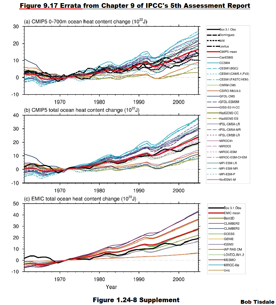
Figure 1.24-8 Supplement
The corrections appear to have changed only the red “CMIP5 mean” curves, raising them so that they are now greater than the observations. Thanks, Nic.
That does not alter the fact that the IPCC’s illustration bears no resemblance to my Figure 1.24-7.
[End Update.]
Note: Climate model “drift” is, basically, a phenomenon where the climate model outputs can change with time even if the inputs were to be kept constant. The problem is discussed in Sen Gupta et al. (2013) Climate Drift in CMIP5 Models (paywalled). The abstract reads (my boldface):
Climate models often exhibit spurious long-term changes independent of either internal variability or changes to external forcing. Such changes, referred to as model “drift,” may distort the estimate of forced change in transient climate simulations. The importance of drift is examined in comparison to historical trends over recent decades in the Coupled Model Intercomparison Project (CMIP). Comparison based on a selection of metrics suggests a significant overall reduction in the magnitude of drift from phase 3 of CMIP (CMIP3) to phase 5 of CMIP (CMIP5). The direction of both ocean and atmospheric drift is systematically biased in some models introducing statistically significant drift in globally averaged metrics. Nevertheless, for most models globally averaged drift remains weak compared to the associated forced trends and is often smaller than the difference between trends derived from different ensemble members or the error introduced by the aliasing of natural variability. An exception to this is metrics that include the deep ocean (e.g., steric sea level) where drift can dominate in forced simulations. In such circumstances drift must be corrected for using information from concurrent control experiments. Many CMIP5 models now include ocean biogeochemistry. Like physical models, biogeochemical models generally undergo long spinup integrations to minimize drift. Nevertheless, based on a limited subset of models, it is found that drift is an important consideration and must be accounted for. For properties or regions where drift is important, the drift correction method must be carefully considered. The use of a drift estimate based on the full control time series is recommended to minimize the contamination of the drift estimate by internal variability.
In other words, because of model flaws, climate model outputs are adjusted by climate scientists when simulating the deep oceans. Let’s rephrase that: Because of inherent flaws in climate models, when examining model performance, climate scientists will adjust the outputs of climate models before comparing them to data. How bizarre is that?
LET’S RETURN TO OUR TOA ENERGY IMBALANCE-BASED OCEAN HEAT CONTENT AND ELIMINATE THE OUTLIERS (FULL OCEAN)
Three of the 21 models in Figure 3.24-7 are showing way too much heat accumulation, and 5 of the models show the oceans losing heat because of their negative TOP-OF-THE-ATMOSPHERE energy imbalances. They are so far from the much-adjusted observations I’ve excluded them in Figure 1.24-9.

But eliminating the outliers creates other problems for the models. With the obvious outliers removed, not one of the remaining 13 models has an ocean heat content trend that’s lower than the observed trend. In other words, all of the models are showing too much warming. And that means, for most the remaining models, the climate sensitivities to CO2 are too high.
With the outliers removed, according to the model mean, the models are showing a heat accumulation that’s more than 2 times higher than observed.
WHAT ABOUT THE GISS MODEL E2 SIMULATIONS FROM THE CMIP5 ARCHIVE (FULL OCEAN)?
For a number of years, Gavin Schmidt (the director of the Goddard Institute of Space Studies, GISS) presented model-data comparisons at RealClimate that included simulated and observed ocean heat content for different depths. Gavin compared models and data for the depths of 0-700 meters in the posts that appeared in December 2009, May 2010, January 2011 and February 2012. It was only in the last post that Dr. Schmidt presented the comparison for the modeled full ocean and data for 0-2000 meters. We’ll illustrate the model-data comparison for the top 700 meters in a moment, but let’s first stick with the data for the top 2000 meters and the modeled ocean heat accumulation for the full oceans.
You’ll note that the ocean heat content graphs in those RealClimate posts have been corrected per Gavin’s May 2012 post OHC Model/Obs Comparison Errata. The ocean heat content comparisons in them used the GISS models from the earlier CMIP3 archive. Gavin Schmidt closed his errata post with:
Analyses of the CMIP5 models will provide some insight here since the historical simulations have been extended to 2012 (including the last solar minimum), and have updated aerosol emissions. Watch this space.
I suspect some of you, like me, have been patiently waiting for those CMIP5-archived GISS Model E2-based model-data comparisons for ocean heat content. Yet, for more than four years, none have been posted at RealClimate.
For those interested, Figure 1.24-10 compares the data with the top-of-the-atmosphere energy imbalance-based ocean heat content for the three GISS Model E2-R simulations…along with the mean of those 3 runs. The “R” suffix letter stands for the Russell Ocean model that’s coupled to the GISS Model E.

This batch of GISS climate models is showing that they are too sensitive to CO2 by a wide amount. The modeled heat accumulation shown by the model mean of this GISS model more than doubles that shown by the data.
Looking at the legends in Figures 1.24-6, -7 and -9, you’ll note that GISS also has another group of model experiments with an “H” suffix. The “H” stands for HYCOM ocean. Figure 1.24-11 includes the model-data comparison of the GISS models with the HYCOM oceans.

Once again, the GISS models show they are way too sensitive to CO2. The model mean of this GISS model shows a heat accumulation that’s more than twice the observations.
I’ll let you speculate about why there have been no model-data comparisons of ocean heat content at RealClimate for 4 years.
MODEL-DATA FOR 0-700 METERS
We’ll be using the annual NODC ocean heat content data (0-700m) here in the following comparisons. For the comparisons I’ve simply shifted the data so that the 1955 value is zero.
There is better sampling at the depths of 0-700 meters than at 700-2000 meters before the ARGO era, so the NODC ocean heat content data for the depths of 0-700 meters is a better dataset. While sampling at these upper depths may be better globally, they were still very poor in the southern hemisphere before the deployment of the ARGO floats. With that in mind…
For these comparisons we’ll rely on the IPCC’s statement that “The upper ocean (0-700 m) accounts for about 64% of the total energy change inventory…” from the earlier quote. That is, we’re taking the scaling factor (1.61*10^22 Joules/year per watt/m^2) and multiplying it by 0.64 to determine the annual ocean heat content uptake for the top 700 meters of the oceans from the top-of-the-atmosphere energy imbalance. The following are the pertinent graphs without commentary, because the comments would basically be the same as those for the full oceans.

# # #

# # #

# # #

# # #

# # #

CLOSING
The energy imbalance at the top of the atmosphere and ocean heat accumulation are crucial elements in the hypothesis of human-induced global warming. Because there is no agreement among the climate models about the energy imbalance at the top of the atmosphere (Figure 1.24-1), there can be no agreement among the climate models about the heat accumulating in the oceans (Figures 1.24-7 and 1.24-14).
With the unlikely outliers removed, or referring to the GISS Model E2-R and GISS Model E2-H simulations, the differences between the observed and modeled ocean heat accumulation indicate the models are much too sensitive to the hypothetical impacts of CO2.
With the outliers removed, according to the model mean, the models are showing a heat accumulation that’s more than twice the observed heat accumulation for the depths of 0-700 meters and for the full oceans. And depending on the GISS climate model and depth, the modeled heat accumulation can be two to almost three times higher than what has been observed.
In the models used by the IPCC for their 5th Assessment Report, many of the modeled oceans are not storing heat close to the (much-adjusted) observed rates, so those models are not simulating global warming as it exists on Earth. But there’s really nothing new about that. We can simply add ocean heat accumulation and top-of-the-atmosphere energy imbalance to the list of things that climate models do not simulate properly: like surface temperatures, like precipitation, like polar sea ice, like polar amplification, like El Niño and La Niña processes, like the Atlantic Multidecadal Oscillation, like the Pacific Decadal Oscillation, and so on.
Once again, climate models have shown they are good for one thing and one thing only: to display how poorly they simulate Earth’s climate.
Important Note: As discussed, because of inherent flaws in climate models like model drift, when examining model performance, climate scientists will adjust the outputs of climate models before comparing them to data.
THANKS
This chapter is based on my blog post Climate Models Fail: Global Ocean Heat Content (Based on TOA Energy Imbalance). As you’ll note in that post, I purposely used the wrong scaling factor for converting the top-of-the-atmosphere energy imbalance to ocean heat uptake. I did that because I found it odd that the trends of the observations aligned almost perfectly with the trends of the model mean for the full oceans and for the top 700 meters. While it’s likely only a coincidence, it appeared as though the models were tuned to the wrong scaling factor.
Many thanks to Willis Eschenbach and Roger Pielke, Sr. for their comments on the initial (but much different) drafts of that blog post and to researcher Nic Lewis for his comments on the thread of the cross post at WattsUpWithThat.
ABOUT THE ERRONEOUS TRENDS LISTED ON THE BOOK ILLUSTRATIONS
I noted above that this chapter was based on the blog post Climate Models Fail: Global Ocean Heat Content (Based on TOA Energy Imbalance), where I had purposely used the wrong scaling factor for converting the top-of-the-atmosphere energy imbalance to ocean heat uptake. If you were to compare the trends shown in that original blog post to the trends listed in Chapter 1.24 of my ebook On Global Warming and the Illusion of Control – Part 1, you’d note that I updated some of the trends in the book, but not all. My apologies.
The trends listed on the illustrations in this post fall into line with what we would expect when compared to the trends listed in the original post. That is, they are approximately 1.41 times higher.
NEXT IN THE SERIES
We’re going to take a look at the 8 outlying climate models presented in this post and discuss an important aspect of their outputs.
Bob – when you say “when examining model performance, climate scientists will adjust the outputs of climate models before comparing them to data” do you mean that they ‘unofficially’ compare the models to data in order to find the difference, then they adjust the models to remove the difference, then they ‘officially’ compare the models to data.
Mike, I don’t know how climate scientists determine which models have problems with “drift”, and, in turn, which model outputs need to be adjusted.
Correcting model drift before comparing to observations? OMG! How, pray tell, is one to test the bleeping model? Sounds rather like the old Texas Marksman insult of designating the target after the hit.
Tom, on at least one occasion, climate scientists have also adjusted surface temperature data before comparing them to models. See Roger Pielke, Sr’s post “Comments On The Paper “Skillful Predictions Of Decadal Trends In Global Mean Surface Temperature” By Fyfe Et Al 2012”:
https://pielkeclimatesci.wordpress.com/2012/04/24/comments-on-the-paper-skillful-predictions-of-decadal-trends-in-global-mean-surface-temperature-by-fyfe-et-al-2012/
There Roger, Sr. writes:
“This is quite an amazing admission. They write that the ‘model does not reproduce long-term trends’ than ‘a linear trend correction may be required’ and ‘we correct for systematic long-term trend biases.’ The model results are tuned. They are not ‘freecasts’.”
…Ummmm, doesn’t that defeat the purpose of the model ????
Depends on what the “purpose” of the model is.
Given that we have satellite data for TOA incoming and outgoing radiation, I am curious about why we need models. Judith Curry quotes JoNova:
Exactly so. In any event, Judith Curry’s blog post is well worth reading.
Computers and electronic sensors are going to be the death of us all.
In the old days someone read a number from a thermometer and recorded it on a sheet of paper.
Now an electronic sensor takes a voltage reading, converts it to a binary number, runs it through an algorithm and writes it to electronic memory. Then later someone comes along and runs more algorithms against the numbers in storage, changes them, then replaces them. Then this process gets repeated multiple times.
Then another program takes all these numbers, estimates missing numbers and calculates an average global temperature to a hundredth of a degree.
And with all the new supercomputers, we can draw all kinds of pretty pictures showing, to the hundredth of a degree, just how hot and cold it is on the globe at any given time.
Ain’t technology wonderful?
No matter what kind of thermometer you are using it should still be subject to calibration. The whole process should have a defined audit trail.
Notwithstanding the above, the one advantage paper records have is that it is more obvious if they have been doctored.
…If you torture the data long enough, it will confess to anything !
Reblogged this on gottadobetterthanthis and commented:
–
If simulation models for engineers worked so poorly, there would be a lot of lawsuits and a lot of engineers in jail.
I’m always curious about this, too. What is the class that you ever took where averaging all the wrong answers and submitting that value was accepted? Must have been different colleges than the ones I attended. Why, Bob, are they allowed to pitch that approach with climate model outputs?
Differences between diffuse and condensed wave radiation could also have greater impact on overall models?
So what is the difference between diffuse and condensed wave radiation ??
What is condensed wave radiation ? Condensed in what sense ?
g
Bob T. excellent post, well researched and logically presented, as always. One question however; Should this…
===================
“In the models used by the IPCC for their 5th Assessment Report, many of the modeled oceans are not storing heat close to the (much-adjusted) observed rates, so those models are not simulating global warming as it exists on Earth.”
===================
possibly read better as…
“In the models used by the IPCC for their 5th Assessment Report, many of the modeled oceans are storing FAR GREATER HEAT then the (much-adjusted) observed rates, so those models are not simulating global warming as it exists on Earth.”
The rest of this excellent paragraph clarifies which direction the models are wrong in, but I do not like to leave the CAGW advocates room to misinterpret.
Thanks again for your work.
David A, I’ve left the text the same in the post, but I’ve revised it in the final for the book…to be reissued later this year. Thanks.
First off a discussion of units.
A watt is a metric unit of power, energy over time, not energy per se. The metric energy unit is the joule, English energy unit is the Btu. A watt is 3.412 Btu per English hour or 3.600 kilojoule per metric hour.
In 24 hours ToA power of 340 W/m^2 will deliver 1.43 E19 Btu to a spherical surface with a radius of 6,386 km. The CO2 RF of 2 W/m^2 will deliver 8.39 E16 Btu, 0.59% of the ToA.
At 950 Btu/lb of energy, evaporating 0.74 inches of the ocean’s surface would absorb the entire ToA, evaporating 0.0044 inches of the ocean’s surface would absorb the evil unbalancing CO2 RF.
More clouds. Big deal.
ToA spherical surface area, m^2……………5.125.E+14
W = 3.412 Btu/h……………………………………3.412.E+00
ToA, 340 W/m^2, Btu/24 h……………………1.43E+19
CO2 RF, 2 W/m^2, Btu/24 h…………………..8.39E+16
Ocean surface , m^2………………………………3.619E+14
m^2 = 10.764 ft^2………………………………….1.076E+01
Ocean surface, ft^2………………………………..3.895E+15
Water density, lb/ft^3………………………….62.4
Lb of water in 1 foot of ocean………………..2.431E+17
Evaporation, Btu/lb……………………………950.0
Amount of ocean evaporation
Feet needed to absorb ToA…………………..0.062
Inches needed to absorb ToA………………..0.74
Feet needed to absorb CO2 RF………………0.0004
Inches needed to absorb CO2 RF…………..0.0044
OK then. How about we stick to SI units and avoid imperial yesteryear cross-dressing, Hiroshima bombs and whatever other whacko PR claptrap is out there? Then we can discuss dimensional consistency issues with a little more clarity.
Christ yes, never do a calculation in beer bottles or Manhattans.
“How about we stick to SI units and avoid imperial yesteryear cross-dressing”
Well, because we here in the US don’t use the worthless metric system. We tried it once and it just didn’t work out. So give me the inches, feet, acres, Fahrenheit, watts and it will all work out for the best. Why should we have to convert everything?? Time for everyone outside the US to do their fair share.. for a change.
BTW watts is SI. I warn my engineering students to make certain they use English hours w/ Btu and SI hours w/ kJ.
1) Anthro CO2 is trivial.
2) CO2 RF is trivial.
3) GCMs don’t work.
All the rest is academic, besides the point, sound & fury signifying nothing.
I guess I am forced to use the /sarc tag from this point on. Everytime (I think anyway) that a posting is really so outrageous everyone will take it as a joke, it is taken literally. Oh well, that is why we are all different. /sarc
Yeah but once upon a time you lot tried imperial too. Some skin-flint liquor salesman managed to screw around with fluid ounces per pint so that didn’t work out so well either. Now you want to adopt watts in lieu of Btu/hr. Anyone would think you have sovereignty issues or think Joules sounds too much like some wrinkly old butler. Meanwhile climate doomsters regularly hop from energy to flux to temp faster than the speed of green light in furlongs per metric hour. So let’s all standardise on spades of baloney per hair clump as the internationally accepted scientific unit of hypothetical cause adherence. Gotta run, delivery of a baker’s dozen 8′ x 4′ sheets of 19mm ply just arrived.
Agree – life is too short to vast on non-SI units – besides, non-SI units are potentially fatal.
(SI = International System of Units)
“The peer review preliminary findings indicate that one team used English units (e.g., inches, feet and pounds) while the other used metric units for a key spacecraft operation.”
MARS CLIMATE ORBITER – UNIT MISMATCH
Three nations have not officially adopted the International System of Units as their primary or sole system of measurement: Burma, Liberia, and the United States. The metric system has been officially sanctioned for use in the United States since 1866, but the US remains the only industrialised country that has not adopted the metric system as its official system of measurement.
Well I think that BTU is only a unit of ” heat ” energy. In fact I think the T in BTU stands for Thermal; meaning heat.
G
And joule (J) is an SI unit, not a metric unit.
The Pyramid Inch is only used for foretelling history from the passage in the Great Pyramid. (marks on the walls)
Would I be correct in believing the converting the temperature to joules is to end up with big scary numbers of zeros, 10^22 is clearly far more scary then 10^-2, right?
So why don’t they go the whole hog and use ergs? That way they could get a really scary 10^29!
…Is it just my computer or does the rating system no longer function ?
mine as well…
…OMG, we’ve been derated ! LOL
berated, derated, now deflated.
Yeah, it looks like it’s been turned off.
Hi Bob
Thanks for this helpful post. I have three initial comments.
1. You show the ocean heat content Figure 9.17 from the AR5 report. I discovered a few months ago that this figure was wrong in the original report, which I believe is the version you show. I don’t think this is generally realised.It was corrected in the 17 April 2015 WG1 errata file, page 10. The change to the CMIP5 mean for total OHC is large it ends up 50% higher than in the AR5 report. I think this was a simple error, and nothing to do with adjusting for drift in the control run.
2. You show the values for GISS-E2-R p1, p2 and p3. These are different versions of the model: NINT, TCAD and TCADI respectively, with different treatment of atmospheric chemistry and aerosols. They have different TCR and ECS values, so one would not expect them to have the same ocean heat content changes. Six historical runs were carried out for each model version; the inter-run variation in cumulative OHC change is quite small for both the NINT and TCADI versions, and I assume also for TCAD. I presume your values are means for each six run ensemble. Historical simulation OHC changes in GISS-E2-R p1 (NINT) are given on the GISS website (see Marvel et al 2015 page). They are only ~86% of the change in TOA radiative imbalance, not ~93%, on my calculations. It is possible that the OHC values Marvel et al derived are incorrectly calculated, or (I think less likely) that my TOA values are. Note that, even without deducting the control run mean TOA radiative imbalance, I get somewhat different values from yours.
3. In AR5 Fig. 9.17, simulation drift was supposedly removed from all CMIP5 runs by deducting a contemporaneous portion of a quadratic fit to each corresponding pre-industrial control run. I agree that removal of simulation drift in terms of heat uptake, a flow variable, is very questionable. There seems to be little or no coherence in annual to centennial variability between periods in a control run after another simulation has been branched off it and variability in the corresponding part of the branched-off simulation, in cases I have looked at.
However, I think there is considerable persistence of the offset from zero in heat uptake, which corresponds to a drift in heat content. So, whilst I disagree with the IPCC treatmetn, I think ignoring the drift in heat content gives a biased view. It is not clear that modest radiative imbalance in the piControl run (e.g., arising from energy leakage) has serious implications for simulations by a model of climate change, although it might have an effect if the imbalance is in fact temperature dependent.
Thanks, Nic. I’ve provided an update with the corrected IPCC Figure 9.17.
Drift is a major problem in the models, Nic. They need to address it, not fiddle with the outputs.
Bob, I agree that drift is a big problem is some models. But a model can have a TOA radiative imbalance in its preindustrial control run that arises from energy leakage and does not cause any drift in GMST or in its ocean heat content. Such energy leakage, due for instance to imperfect treatment of the boundary between the atmospheric and ocean grids, may be difficult to eliminate entirely. If it is small and not very sensitive to temperature, it is not obvious that it will affect a model’s performance.
I wonder if it is possible to model the cyclic temperature pattern seen in reconstructions of our current interglacial period using ENSO processes that are made to run on a millennial time scale. Obviously ocean storage and release of solar heat is the source of that pattern. From that model we can develop an estimate of how much heat the oceans store while the Earth cools and how much heat the oceans give up as Earth warms. I would use water vapor from evaporation as the source of greenhouse gasses at work during oceanic solar energy loss to the atmosphere, and loss of water vapor greenhouse affect during oceanic solar energy storage. Theo would add that the fine scale of the earlier piece of these reconstructions will be quite different compared to the later pieces of these reconstructions.
Again, I have to go with what is a known process to induce a temperature spike. El Nino. So the simple millennial model would use a preponderance of stable windless El Nino’s disgorging an ocean full of heat. For that to happen there had to have been a long previous condition whereby clear skies allowed solar energy to penetrate and windy Easterly conditions to keep that energy mixed in, which by the way is the normal state (La Nada normal, and La Nina super normal). At some point in time, the oceans would be at their peak in terms of absorbing solar energy. At that point in time, oceanic/atmospheric teleconnections would work in concert to stall the Easterlies, allowing the ocean to layer up and begin to disgorge that heat. And as long as there is heat, it will continue, nearly unabated to disgorge that heat till depleted, leaving land flora and fauna basking in a warm moist world till the atmosphere is also depleted of that blanketed warmth. Unfortunately, that warmth heralds a coming fall into a necessary but killing frigid Earth that allows the oceans to regain their store of heat.
Looking for exotic reasons for climate change reminds me of the oft repeated and very wrong statement that weather and climate are two different things. To dismiss ENSO on a large scale makes the same error. It seems reasonable to me to look at fine scale ENSO processes that we know change our short term measured temperatures on yearly and even decadal scales, as the same process at work on an interglacial scale.
Nice post. A different way to show that models run hot. Unfortunately only the ARGO era has sufficient data reliability for this to be convincing, a shorter period than satellite atmosphere estimates. But for that era, still a confirmation.
That is odd, I thought that they were using the models to adjust the Data to fit the Models, not the other way around.
Thanks Bob!
Is the actual data even saying anything here with short date ranges in the presence of long period cycles? Many of these ocean cycles are relatively recent discoveries in climate science and the focus should be on better understanding of them.
Thank you Bob,
Have you looked at the model-hindcasting/fabricated-aerosol issue, as described below? I would be interested in your comments.
Hypothesis:
The climate models cited by the IPCC typically use values of climate sensitivity to atmospheric CO2 (ECS) values that are significantly greater than 1C, which must assume strong positive feedbacks for which there is NO evidence. If anything, feedbacks are negative and ECS is less than 1C. This is one key reason why the climate models cited by the IPCC greatly over-predict global warming.
I reject as false the climate modellers’ claims that manmade aerosols caused the global cooling that occurred from ~1940 to ~1975. This aerosol data was apparently fabricated to force the climate models to hindcast the global cooling that occurred from ~1940 to ~1975, and is used to allow a greatly inflated model input value for ECS.
Some history on this fabricated aerosol data follows:
http://wattsupwiththat.com/2009/06/27/new-paper-global-dimming-and-brightening-a-review/#comment-151040
More from Douglas Hoyt in 2006:
http://wattsupwiththat.com/2009/03/02/cooler-heads-at-noaa-coming-around-to-natural-variability/#comments
Regards, Allan
Ocean heat uptake is wrong in most models because they neglect a temperature dependence of a latent heat of water vaporization. This results in a 2.5% overestimation of an ocean energy loss by evaporation from tropical seas.
If I’m not misteaken (often so) you can correct the latent heat of vaporization for Temperature very simply by just adding the Temperature difference from the boiling point.
So if it is 590 Calories per gram at 100 deg. C, then it should be about 690 cal per gram at zero deg, C, which is just how much energy it takes to raise the ice water to the boiling point and then evaporate it.
I believe that gets you close to the table numbers.
G
Yes, but the problem runs deeper, according to Gavin: ” If the specific heats of condensate and vapour is assumed to be zero (which is a pretty good assumption given the small ratio of water to air, and one often made in atmospheric models) then the appropriate L is constant (=L0).”
https://judithcurry.com/2012/08/30/activate-your-science/#comment-234131
It is that “pretty good assumption” that forces a 2.5% error. Unfortunately, Gavin did not supply an estimate of consequences of that assumption. In my estimate it limits the reliability of “most atmospheric models” to 100 hours of simulated time.
Way back in the day when Jimmy Hansen was “promoted” Chief of GISS he had spent about 10-years failing to “model” the “climate” i.e. meteorology of Venus (Carl Sagan beat him badly on that). So when Jimmy quickly turned to “climate change earth” my guess is most of the Venus code became the “physics” of the “Climate Change” models that are here with us today. Failure is as failure does.
Ha ha
The current set of models are fundamentally incorrect. The cult of CAGW have hand waved away 18 years without warming at time in which anthropogenic CO2 is increasing year by year. Significant unequivocal cooling will be a game changer and a top media item.
It appears the cooling has started. If solar cycle changes were the cause of the warming in the last 150 years, global warming is reversible and we could see global cooling of 0.8C with the most amount of cooling occurring in the 40 to 60 degree latitude region. Reverse of the warming, return to conditions in the Little Ice age.
Regions of the ocean, 40 to 60 degree latitude, were roughly 10C colder during the Little ice age which explains why the Thames River froze and why there was record snowfall and expanding glaciers. A hint that the warming in the last 150 years had nothing to do with anthropogenic CO2 emissions is CO2 warming if the CO2 mechanism was not saturated would be global as CO2 is more or less evenly distributed in the atmosphere so there is no reason for super warming 40 to 60 degree latitude.
The cult of CAGW did not understand that the delay in the onset of solar cycle cooling (there was no cooling when the solar cycle initially slowed down) is due to a large scale change in the sun and due to solar wind bursts. The delay in cooling is observational proof that there is a large scale change occurring to the sun.
GCR is now the highest ever recorded for this period in a solar cycle. Wind speed is starting to increase over the ocean in the 40 to 60 degree latitude region which causes increased evaporation cooling. The solar coronal holes are starting to dissipate which is interesting.
Comments:
GCR is an abbreviation for galactic cosmic rays which is the silly name physicist gave for high speed cosmic protons. (The initial discovers thought the phenomena was a new type of ‘ray’, rather than a particle and physicists did bother to correct the idiotic name. The high speed cosmic particles are also called galactic cosmic flux GCF.)
The GCR strike the earth’s atmosphere and create cloud forming ions. The modulating effect on planetary clouds is greatest in the 40 to 60 degree latitude region. The geomagnetic field deflects the GCR at lower latitudes. At higher latitudes due to the orientation of the geomagnetic field GCR is not blocked and hence is sufficiently high than more or less GCR does not affect cloud formation.
The number and speed of GCR (galactic high speed protons) are modulated by the ‘strength’ and extent of the solar heliosphere. The solar heliosphere is name given for a tenuous plasma of gas and pieces of magnetic flux that ejected from the sun. The solar heliosphere blocks, deflects, and slows down the galactic high speed protons, so when the solar cycle is active there are less high speed protons striking the earth and vice versa.
Complicating the solar modulation of planetary temperature are three additional mechanisms.
Solar wind bursts create a space charge differential in the earth’s ionosphere which in turn cause there to be a current flow from high latitude regions of the planet (also the 40 to 60 degree latitude region) to the equator. This current flow changes cloud properties in both regions (40 to 60 degree latitude region) and the equatorial region which cause warming at both locations when there are large number of regular solar wind bursts.
The solar wind bursts are primarily caused by coronal holes, not sunspots. The coronal holes are persistent and can last for months. The coronal holes are not taken into account with the sunspot count so the appears of coronal holes and solar wind bursts. The solar wind bursts will cause warming even when GCR therefore making appear that a high GCR will not cause cooling. A high GCR will cause cooling if there are no solar wind bursts.
The third mechanism is changes to total solar irradiation (TSI). It will be interesting to see if there is an anomalous drop in TSI, due to the interruption in the solar cycle. I suspect there will be an anomalous drop in TSI.
The fourth mechanism is interesting as it takes roughly a decade to change and carries over from solar cycle to solar cycle. This a net charge mechanism that affects wind speed and precipitation. The fact that jet wind speed is starting to increase is observational proof that the delay in the change of that mechanism is almost over.
http://www.ospo.noaa.gov/data/sst/anomaly/2016/anomnight.2.29.2016.gif
Typo?
10C? Don’t you mean around 1C? If it was 10 c colder we would be talking a major ice age. The Thames would unlikely freeze today like in the past because building around it has increased it’s flow.
http://www.seafriends.org.nz/issues/global/cet-1659.gif
The CET has warmed around 1.5 c since the LIA and mainly during winter.
Major problems with the claimed ocean warming and no wonder the models are hopelessly wrong.
Firstly, how can the warming of oceans be greater than all energy in the atmosphere?
Energy in the atmosphere 5×10^21 J/K.
http://i772.photobucket.com/albums/yy8/SciMattG/atmosphere-vs-ocean-heat-capacity2_zpsjjwuhpbk.jpg
The oceans energy content is 5.6×10^24 J/K.
The 4% greenhouse effect of CO2 in all the atmosphere leads to 2×10^18 J/K.
BUT, the human content of CO2 is only around 3.4% of this at 6.8×10^16 J/K.
Secondly, how does 6.8×10^16 J/K magically become 10^22 J/K?
The ocean energy is 82,352,941 times larger than this 6.8×10^16 J/K.
The ocean warms down to below 100M thanks to the overwhelming shortwave radiation directly from the sun. Long-wave radiation only penetrates less than a mm of the oceans surface.
Therefore even 82 million times more energy in the ocean is far too small because the gigantic majority is warmed by solar energy.
Even if we take this as a mm, it is still 100,000 times smaller than the depth solar energy warms.
Hence,
Thirdly, proportionally the oceans energy is 8,235,294,100,000 times greater than 6.8×10^16 K/J has on 1mm of the ocean depth.
This shows without doubt that it is impossible for CO2 to warm the ocean and be noticeable, even over the next 10,000 years.
…But Matt, models can do anything !!
I posted a comment on the Milton Freidman thread which has some bearing on the point you make and the suggestion that
My comment read:
A lot of interesting information.
You state:
Even the figure of 100 microns is too large.
As you will note from the plot set out below, only about 17% of LWIR can penetrate vertically as deep as 100 microns, and 60% is absorbed within 3 microns. But of course, DWLWIR is not a vertical source, but rather it is omnidirectional, and this has a significant impact upon its penetration in a vertical column.
Much of the DWLWIR is interacting with the ocean not vertically, but at a grazing angle of say 10deg and less, or 20deg or less, or 30 deg or less. This means that about 80% of all DWLWIR is absorbed within a vertical depth of just a few microns.
Ocean overturning, is a diurnal phenomena, and does not operate 24/7, the action of the wind, waves, swell are slow mechanical processes especially in light wind conditions (say BF3 or less) and it is difficult to see how these slow mechanical processes can mix and sequester to depth, the DWLWIR absorbed within the 3 micron layer, and hence to dilute that energy by volume, at a rate which would prevent the rapid evaporation of the surface layer brought about the energy that is being absorbed within the 3 micron layer. It is difficult to see how increased DWLWIR can effectively warm the oceans given that it would appear that it drives evaporation at the surface, and therefore if anything it goes to cool the surface layer.
That is I how I see the the skin temperature, but there is a argument that all it does is increase the evaporation at the surface and latent heat becoming a negative feedback.
One of the issues is that radiation is from the surface, but absorption of energy is at depth such that it is not surprising that there may from time to time be some imbalance.
Ignoring the variable heat content of the top layer of the ocean which can vary significantly on decadal or multidecadal periods, and therefore have an impact upon radiative imbalance at any given time, but rather consider the implications of the claim that energy absorbed in the very surface layer of the ocean is effectively mixed into the ocean and thereby finds its way in to the mid to deep ocean.
IF CO2 did anything of real significance, why is the mid to deep ocean so cold after some 4 billion years (or so) of solar plus DWLWIR?
I would like to know why the mid to deep ocean is so cold after it has received all this energy (solar + DWLWIR) for such a lengthy period.
An ice age involves freezing of only a relatively small depth of the ocean, and once the surface has frozen, the ice acts like a lid so that energy/heat in the mid to deep ocean is contained there ready for the receipt of further input once the ice age passes.
This conclusion is taking into account the warming of 6.8×10^16 K/J at the surface from CO2, so I’ve not ignored the variable heat content at the top of the ocean. It is just that it so small compared to the energy heat content of the ocean, it is like adding an elephant to the planet every so often and then trying to weight the planets mass to see if there is any difference. It is thousands of billions times smaller than the ocean heat content so mixing makes it disappear as though it never occurred.
The ocean top 100 feet can be mixed greatly at times especially with strong storms, but depths between 100 and 400 feet mainly require ocean surface currents. Below this depth only very select spots related to ocean thermohaline circulation sink to deeper depths. Therefore the huge ocean remains cold at 4 c because there is limited interaction between the surface and the depths other than the currents mentioned. With the ocean being so huge compared to the limited currents, upwelling and sinks, it absorbs any energy thrown at it as though it was not even there.
The ice age mechanism is very complicated and still unknown, but when the cold ocean at 4 c mainly becomes near or at the surface away from the Tropics, then we have our Ice age. The biggest concerns humans face regarding changes, are the significant cooling in the oceans recently between 40-60N and 40-60S. The source in the North Atlantic is remaining strong, yet the cooling has increasingly spread outwards and reached the UK recently for the first time too. The coldest anomalies are now becoming part of the main NAD current and are moving towards Norway.
The only way to see a difference over hundreds of years from 6.8×10^16 K/J is if it remained near the surface and didn’t mix with the rest of the ocean.
I have often pointed out that the reason we have ice ages is because the ocean below the upper layer is so cold. This coldness comes back to haunt.
I have often suggested that it is incorrect to assess the average temperature of the Earth by using the surface temperature of the ocean, This gives a false perspective as to how warm the planet is.
This may be fine for the land surface, after all the ground gets warmer with depth (it being heated from below), but it is inapplicable with the oceans. It is only just by chance that we are today seeing ocean average surface temperature around say 20degC. In a different era this could easily be far less and not due to any change in incoming radiative budget but simply because the cooler lower layers have impacted and come back to bite.
It would be more appropriate to consider the average temperature of the Earth by taking some account of the average temperature of the ocean, which as you note is more in the region of 4degC.
In that first mm of water being diffuse by wind chop or directly condensed into a glass surface sea.
Not to mention variable cloudiness, I mean if you’re modeling ratios between top of the sky and surface of the ocean, do you just paste over those things as ineffectual or hard variables, or is that considered as something in the middle of the model sandwich?