Guest essay by Ferdinand Engelbeen
Both Bart Bartemis and Dr. Murray Salby are confident that temperature is the only/main cause of the CO2 increase in the atmosphere. I am pretty sure that human emissions are to blame. With this contribution I hope to give a definitive answer…
1. Introduction.
Some of you may remember the lively discussions of already 5 years ago about the reasons why I am pretty sure that the CO2 increase in the atmosphere over the past 57 years (direct atmospheric measurements) and 165 years (ice cores and proxies) is manmade. That did provoke hundreds of reactions from a lot of people pro and anti.
Since then I have made a comprehensive overview of all the points made in that series of discussions at:
http://www.ferdinand-engelbeen.be/klimaat/co2_origin.html
There still is one unresolved recurring discussion between mainly Bart/Bartemis and me about one – and only one – alternative natural explanation: if the natural carbon cycle is extremely huge and the sinks are extremely fast, it is -theoretically- possible that the natural cycle dwarfs the human input. That is only possible if the natural cycle increased a fourfold in the same time frame as human emissions (for which is not the slightest indication) and it violates about all known observations. Nevertheless, Bart’s (and Dr. Salby’s) reasoning is based on a remarkable correlation between temperature variability and the CO2 rate of change variability with similar slopes:

Capture: Fig.1: Bart’s combination of T and dCO2/dt from WoodForTrees.org
Source: http://i1136.photobucket.com/albums/n488/Bartemis/temp-CO2-long.jpg_zpsszsfkb5h.png
Bart (and Dr. Salby) thinks that the match between variability and slopes (thanks to an arbitrary factor and offset) proves beyond doubt that temperature causes both the variability and slope of the CO2 rate of change. The following will show that variability and slope have nothing in common and temperature is not the cause of the slope in the CO2 rate of change.
2. The theory.
2.1 Transient response of CO2 to a step change in temperature.
To make it clear we need to show what happens with CO2 if one varies temperature in different ways. CO2 fluxes react immediately on a temperature change, but the reaction on CO2 levels needs time, no matter if that is by rotting vegetation or the ocean surfaces. Moreover, increasing CO2 levels in the atmosphere reduce the CO2 pressure difference between ocean surface and the atmosphere, thereby reducing the average in/out flux, until a certain CO2 level in the atmosphere is reached where in and out fluxes again are equal.
In algebraic form:
dCO2/dt = k2*(k*(T-T0) – ΔpCO2)
Where T0 is the temperature at the start of the change and ΔpCO2 the change in CO2 partial pressure in the atmosphere since the start of the temperature change, where pCO2(atm) was in equilibrium with pCO2(aq) at T0. The transient response in rate of change is directly proportional to the CO2 pressure difference between the pCO2 change in water (caused by a change in temperature) and the CO2 pressure in the atmosphere.
When the new equilibrium is reached, dCO2/dt = 0 and:
k*(T-T0) = ΔpCO2
Where k = ~16 ppmv/°C which is the value that Henry’s law gives for the equilibrium between seawater and the atmosphere.
In the next plot we assume the response is from vegetation, mainly in the tropics, as that is a short living response as will be clear from measurements in the real world in chapter 3:

Caption: Fig. 2: Response of bio-CO2 on a step change of temperature
Source: http://www.ferdinand-engelbeen.be/klimaat/klim_img/trans_step.jpg
As one can see, a step response in temperature gives an initial peak in dCO2/dt rate of change which goes back to zero when CO2 is again in equilibrium with temperature. That equilibrium can be static (for an open bottle of Coke) or dynamic (for the oceans). In the latter case one speaks of a “steady state” equilibrium or a “dynamic equilibrium”: still huge exchanges are going on, but the net result is that no CO2 changes are measurable in the atmosphere, as the incoming CO2 fluxes equal the outgoing CO2 fluxes.
Taking into account Henry’s law for the solubility of CO2 in seawater, any in/decrease of 1°C has the same effect if you take a closed sample of seawater and let it equilibrate with the above air (static) or have the same in/decrease in (weighted) average global ocean temperature with global air at steady state (dynamic): about 16 ppmv/°C.
2.2 Transient response of CO2 to an increasing temperature trend.
If the temperature has a slope, CO2 will follow the slope with some delay.

Caption: Fig. 3: Response of bio-CO2 on a continuous increase of temperature
Source: http://www.ferdinand-engelbeen.be/klimaat/klim_img/trans_slope.jpg
A continuous increase of temperature will induce a continuous increase of CO2 with an increasing dCO2/dt until both increases parallel each other and dCO2/dt remains constant. This ends when the “fuel” (like vegetation debris) gets exhausted or the temperature slope ends. In fact, this type of reaction is more applicable to the oceans than on vegetation, but this all is more about the form of the reaction than what causes it…
A typical example is the warming from the depth of a glacial period to an interglacial: it takes about 5,000 years to reach the new maximum temperature and CO2 lags the temperature increase with some 800 +/- 600 years.
2.3 Transient response of CO2 to a sinusoid.
Many changes in nature are random up and down, besides step changes and slopes. Let’s first see what happens if the temperature changes with a nice sinus change (a sinusoid):

Caption: Fig. 4: Response of bio-CO2 on a continuous sinusoidal change in temperature
Source: http://www.ferdinand-engelbeen.be/klimaat/klim_img/trans_sin.jpg
It can be mathematically explained that the lag of the CO2 response is maximum pi/2 or 90° after a sinusoidal temperature change [1]. Another mathematical law is that by taking the derivatives, one shifts the sinusoid forms 90° back in time. The remarkable result in that case is that changes in T synchronize with changes in dCO2/dt, that will be clear if we plot T and dCO2/dt together in next item.
2.4 Transient response of CO2 to a double sinusoid.
To make the temperature changes and their result on CO2 changes a little more realistic, we show here the result of a double sinusoid for sinusoids with different periods. After all natural changes are not that smooth…:

Caption: Fig. 5: Response of bio-CO2 on a continuous double sinusoidal change in temperature
Source: http://www.ferdinand-engelbeen.be/klimaat/klim_img/trans_2sin.jpg
As one can see, the change in CO2 still follows the same form of the double sinusoid in temperature with a lag. Plotting temperature and dCO2/dt together shows a near 100% fit without lag, which implies that T changes directly cause immediate dCO2/dt changes, but that still says nothing about any influence on a trend. In fact still T changes lead CO2 changes and dT/dt changes lead dCO2/dt changes, but that will be clear in next plot…
2.4 Transient response of CO2 to a double sinusoid plus a slope.
Now we are getting even more realistic, not only we introduced a lot of variability, we also have added a slight linear increase in temperature. The influence of the latter is not on CO2 from the biosphere (that is an increasing sink with temperature over longer term), but from the oceans with its own amplitude:

Caption: Fig. 6: Response of Natural CO2 on a continuous double sinusoidal plus slope change in temperature
Source: http://www.ferdinand-engelbeen.be/klimaat/klim_img/trans_2sin_slope.jpg
As one can see, again CO2 follows temperature as well for the sinusoids as for the slope. So does dCO2/dt with a lag after dT/dt, but with a zero slope, as the derivative of a linear trend is a flat line with only some offset from zero.
This proves that the trend in T is not the cause of any trend in dCO2/dt, as the latter is a flat line without a slope. No arbitrary factor can match these two lines, except (near) zero for the temperature trend to match the dCO2/dt trend, but then you erase the amplitudes of the variability…
Thus while the variability in temperature matches the variability in CO2 rate of change, there is no influence at all from the slope in temperature on the slope in CO2 rate of change.
Conclusion: A linear increase in temperature doesn’t introduce a slope in the CO2 rate of change at any level.
2.4 Transient response of CO2 to a double sinusoid, a slope and emissions.
All previous plots were about the effect of temperature on the CO2 levels in the atmosphere. Volcanoes and human emissions are additions which are independent of temperature and introduce an extra amount of CO2 in the atmosphere above the temperature dictated dynamic equilibrium. That has its own decay rate. If that is slow enough, CO2 builds up above the equilibrium and if the increase is slightly quadratic, as the human emissions are, that introduces a linear slope in the derivatives.

Caption: Fig. 7: Response of CO2 on a continuous double sinusoidal + slope change in temperature + emissions
Source: http://www.ferdinand-engelbeen.be/klimaat/klim_img/trans_2sin_slope_em.jpg
Several important points to be noticed:
– The variability of CO2 in the atmosphere still lags the temperature changes, no matter if taken alone or together with the result of the emissions. No distortion of amplitudes or lag times. Only simple addition of independent results of temperature and emissions.
– The slope of the natural CO2 rate of change still is zero.
– The relative amplitude of the variability is a small factor compared to the huge effect of the emissions.
– The slope and variability of temperature and CO2 rate of change is a near perfect match, despite the fact that the slope is entirely from the slightly quadratic increase of the emissions and the effect of temperature on the slope of the CO2 rate of change is zero…
Conclusion: The “match” between the slopes in temperature and CO2 rate of change is entirely spurious.
3. The real world.
3.1 The variability.
Most of the variability in CO2 rate of change is a response of (tropical) vegetation on (ocean) temperatures, mainly the Amazon. That it is from vegetation is easily distinguished from the ocean influences, as a change in CO2 releases from the oceans gives a small increase in 13C/12C ratio (δ13C) in atmospheric CO2, while a similar change of CO2 release from vegetation gives a huge, opposite change in δ13C. Here for the period 1991-2012 (regular δ13C measurements at Mauna Loa and other stations started later than CO2 measurements):

Caption: Fig. 8: 12 month averaged derivatives from temperature and CO2/ δ13C measurements at Mauna Loa [9].
Source: http://www.ferdinand-engelbeen.be/klimaat/klim_img/temp_dco2_d13C_mlo.jpg
Almost all the year by year variability in CO2 rate of change is a response of (tropical) vegetation on the variability of temperature (and rain patterns). That levels off in 1-3 years either by lack of fuel (organic debris) or by an opposite temperature/moisture change [2]. Over periods longer than 3 years, it is proven from the oxygen balance that the overall biosphere is a net, increasing sink of CO2, the earth is greening [3], [4].
Not only is the net effect of the biological CO2 rate of change completely flat as result of a linear increasing temperature, it is even slightly negative in offset…
The oceans show a CO2 increase in ratio to the temperature increase: per Henry’s law about 16 ppmv/°C. That means that the ~0.6°C increase over the past 57 years is good for ~10 ppmv CO2 increase in the atmosphere that is a flat line with an offset of 0.18 ppmv/year or 0.015 ppmv/month in the above graph.
There is a non-linear component in the ocean surface equilibrium with the atmosphere for a temperature increase, but that gives not more than a 3% error on a change of 1°C at the end of the flat trend or a maximum “trend” of 0.00045 ppmv/month after 57 years. That is the only “slope” you get from the influence of temperature on CO2 levels. Almost all of the slope in CO2 rate of change is from the emissions…
3.2 The slopes.
Human emissions show a slightly quadratic increase over the past 115 years. In the early days more guessed than calculated, in recent decades more and more accurate, based on standardized inventories of fossil fuel sales and burning efficiency. Maybe more underestimated than overestimated, because of the human nature to avoid paying taxes, but rather accurate +/- 0.5 GtC/year or +/- 0.25 ppmv/year.
The increase in the atmosphere was measured in ice cores with an accuracy of 0.12 ppmv (1 sigma) and a resolution (smoothing) of less than a decade over the period 1850-1980 (Law Dome DE-08 cores). CO2 measurements in the atmosphere are better than 0.1 ppmv since 1958 and there is a ~20 year overlap (1960 – 1980) between the ice cores and the atmospheric measurements at Mauna Loa. That gives the following graph for the temperature – emissions – increase in the atmosphere:

Caption: Fig. 9: Temperature, CO2 emissions and increase in the atmosphere [9].
Source: http://www.ferdinand-engelbeen.be/klimaat/klim_img/temp_emiss_increase.jpg
While the variability in temperature is high, that is hardly visible in the CO2 variability around the trend, as the amplitudes are not more than 4-5 ppmv/°C (maximum +/- 1 ppmv) around the trend of more than 90 ppmv. To give a better impression, here a plot of the effect of temperature on the CO2 variability in the period 1990-2002, where two large temperature and CO2 changes can be noticed: the 1991/2 Pinatubo eruption and the 1998 super El Niño:

Caption: Fig. 10: Influence of temperature variability on CO2 variability around the CO2 trend [9].
It is easy to recognize the 90° lag after temperature changes, but the influence of temperature on the variability is small, here calculated with 4 ppmv/°C. For the trend, the CO2 increase caused by the 0.2°C ocean surface temperature increase in that period is around 3 ppmv of the 17 ppmv measured…
3.3 The response to temperature variability and human emissions:
With the theoretical transient response of CO2 to temperature in mind, we can calculate the response of vegetation and oceans to the increased temperature and its variability:

Caption: Fig. 11: Transient response of bio and ocean CO2 to temperature [9][11].
Source: http://www.ferdinand-engelbeen.be/klimaat/klim_img/rss_co2_nat.jpg
The bio-response to temperature changes is very fast and zeroes out after a few years [6], the response to the temperature amplitude is about 4-5 ppmv/°C, based on the response to the 1991 Pinatubo eruption and the 1998 El Niño.
The response of the ocean surface is slower, but stronger in effect. The 16 ppmv /°C is based on the long-term response in ice cores and Henry’s law for the solubility of CO2 in ocean waters (4-17 ppmv /°C in the literature).
In reality, both oceans and the biosphere are net sinks for CO2, due to the increased CO2 pressure in the atmosphere and the biosphere also a net sink due to increased temperature on periods of more than 3 years. That is not taken into account here, but is used in the calculation of the net increase of CO2 in the atmosphere with the introduction of human emissions.
If we introduce human emissions , that gives a quite different picture of the relative dimensions involved:

Caption: Fig. 12: Human emissions + calculated and measured CO2 increase + transient response of bio and ocean CO2 to temperature [9][11].
Source: http://www.ferdinand-engelbeen.be/klimaat/klim_img/rss_co2_emiss.jpg
The influence of temperature both in variability and increase rate is minimal, compared to the effect of human emissions, based on the transient response of oceans and biosphere and the calculated decay rate of human emissions.
The long tau (e-fold decay rate) of human emissions is based on the calculated sink rate (human emissions – increase in the atmosphere) and the increased CO2 pressure in the atmosphere above dynamic equilibrium (“steady state”), which is ~290 ppmv for the current weighted average ocean surface temperature. That is thus ~110 ppmv above steady state and that gives ~2.15 ppmv net sink rate per year. For a linear response, the e-fold decay rate can be calculated:
disturbance / response = decay rate
or for 2012:
110 ppmv / 2.15 ppmv/year = 51.2 years or 614 months.
That the sink process is quite linear can be seen in the similar calculation by Peter Dietze with the figures of 27 years ago [12]:
1988: 60 ppmv, 1.13 ppmv/year, 53 years
Or from earliest accurate CO2 measurements:
1959: 25 ppmv, 0.5 ppmv/year, 50 years
Conclusion: Within the accuracy of the CO2 emission inventories and the natural variability, the decay rate of any extra CO2 above the dynamic equilibrium (whatever the cause) behaves like a linear process…
3.4 The derivatives.
What does that show in the derivatives? First the transient response of the biosphere and oceans to temperature variability:

Caption: Fig. 13: RSS temperature compared to CO2 increase and transient response of natural CO2 (biosphere+oceans) rate of change [9][11].
Source: http://www.ferdinand-engelbeen.be/klimaat/klim_img/rss_co2_nat_deriv.jpg
It seems that the amplitude of the natural variability is overblown, but for the rest both the temperature and the transient response of CO2 are equally synchronized with the observed CO2 rate of change with hardly any slope in the transient response. Thus while all the variability is from the transient response, there is hardly any contribution of oceans or biosphere to the slope in CO2 rate of change.
The overdone amplitude of the natural variability may be a matter of CO2/temperature ratio or a too short transient response time, but that is not that important. The form and timing are the important parts.
Now we can add human emissions into the rate of change:

Fig. 14: RSS temperature compared to CO2 increase and transient response of natural CO2 + emissions rate of change [9][11].
Source: http://www.ferdinand-engelbeen.be/klimaat/klim_img/rss_co2_emiss_deriv.jpg
For an exact match of the slopes of RSS temperature and CO2 rate of change one need to multiply the temperature curve with a factor and add an offset. The match of the slopes of the observed CO2 rate of change and the calculated rate of change from the emissions plus the small slope of the natural transient response needed no offset at all: it was a perfect match. Only the amplitude of the variability was reduced, but that has no effect on the small natural CO2 rate of change slope.
As can be seen in that graph, both temperature rate of change and CO2 rate of change from humans + natural transient response show the same variability in timing and form. That is clear if we enlarge the graph for the period 1987-2002, encompassing the largest temperature changes of the whole period:

Fig. 15: RSS temperature compared to CO2 increase and transient response of natural CO2 + emissions rate of change in the period 1987-2002 [9][11].
Source: http://www.ferdinand-engelbeen.be/klimaat/klim_img/rss_co2_emiss_deriv_1987-2002.jpg
As is very clear in this graph, there is an exact match in timing and form between temperature and the transient response of the CO2 rate of change, as was the case in the theoretical calculations. Where there is a discrepancy between the observed and calculated rates of change of CO2 , temperature shows the same discrepancy, like the 1991 Pinatubo eruption which increased photosynthesis by scattering incoming sunlight.
Conclusion: it is entirely possible to match the slopes and variability by temperature only or by the effect of human emissions + natural variability.
4. Conclusion.
Which of the two possible solutions is right is quite easy to know, by looking which of the two matches the observations.
The straight forward result:
– The temperature-only match violates all known observations, not at least Henry’s law for the solubility of CO2 in seawater, the oxygen balance – the greening of the earth, the 13C/12C ratio, the 14C decline,… Together with the lack of a slope in the derivatives for a transient response from oceans and vegetation to a linear increase in temperature.
– The emissions + natural variability matches all observations. See: http://www.ferdinand-engelbeen.be/klimaat/co2_origin.html
Most of the variability in the rate of change of CO2 is caused by the influence of temperature on vegetation. While the influence on the rate of change seems huge, the net effect is not more than about +/- 1.5 ppmv around the trend and zeroes out after 1-3 years.
Most of the slope in the rate of change of CO2 is caused by human emissions. That is about 110 ppmv from the 120 ppmv over the full 165 years (about 70 from the 80 ppmv over the past 57 years). The remainder is from warming oceans which changes CO2 in the atmosphere with about 16 ppmv/°C, per Henry’s law, no matter if the exchanges are static or dynamic.
Yearly human emissions quadrupled from over 1 ppmv/year in 1958 to 4.5 ppmv/year in 2013. The same quadrupling happened in the increase rate of the atmospheric CO2 (at average around 50% of human emissions) and in the difference, the net sink rate.
There is not the slightest indication in any direct measurements or proxy that the natural carbon cycle or any part thereof increased to give a similar fourfold increase in exactly the same time span, which was capable to dwarf human emissions…
Conclusion: Most of the CO2 increase is caused by human emissions. Most of the variability is natural variability. The match between temperature and CO2 rate of change is entirely spurious.
5. References.
[1] Why the CO2 increase is man made (part 1)
[2] Engelbeen on why he thinks the CO2 increase is man made (part 2)
[3] Engelbeen on why he thinks the CO2 increase is man made (part 3)
[4] Engelbeen on why he thinks the CO2 increase is man made (part 4).
[5] http://bishophill.squarespace.com/blog/2013/10/21/diary-date-murry-salby.html?currentPage=2#comments
Fourth comment by Paul_K, and further on in that discussion, gives a nice overview of the effect of a transient response of CO2 to temperature. Ignore the warning about the “dangerous” website if you open the referenced image.
[6] Lecture of Pieter Tans at the festivities of 50 years of Mauna Loa measurements, from slide 11 on:
http://esrl.noaa.gov/gmd/co2conference/pdfs/tans.pdf
[7] http://www.sciencemag.org/content/287/5462/2467.short full text free after registration.
[8] http://www.bowdoin.edu/~mbattle/papers_posters_and_talks/BenderGBC2005.pdf
[9] temperature trend of HadCRUT4 and CO2 trend and derivatives from Wood for trees.
CO2 and δ13C trends from the carbon tracker of NOAA: http://www.esrl.noaa.gov/gmd/dv/iadv/
CO2 emissions until 2008 from: http://cdiac.ornl.gov/trends/emis/tre_glob.html
CO2 emissions from 2009 on from: http://www.eia.gov/cfapps/ipdbproject/IEDIndex3.cfm?tid=90&pid=44&aid=8
[10] The spreadsheet can be downloaded from: http://www.ferdinand-engelbeen.be/klimaat/CO2_lags.xlsx
[11] The spreadsheet can be downloaded from:
http://www.ferdinand-engelbeen.be/klimaat/RSS_Had_transient_response.xlsx
[12] http://www.john-daly.com/carbon.htm
“a change in CO2 releases from the oceans gives a small increase in 13C/12C ratio (δ13C) in atmospheric CO2, while a similar change of CO2 release from vegetation gives a huge, opposite change in δ13C.
Please explain why this is so.
I would have thought that recently ‘fixed’ organic Carbon would be rather derived from new atmospheric CO2 which is fairly rich in C13,. whereas any old sinks that are now realsesiong it – like fossil or the sea, would be low in C13.
It sees to me you have this exactly the wrong way around.
Leo Smith,
Inorganic carbon has a 13C/12C ratio (δ13C) level around zero per mil. That is the case for the oceans, where the deep oceans are around 0-1 per mil, the oceans surface at 1-5 per mil, due to organics dropping out of the surface into the deep. That is also the case for most carbonate deposits all over the world and most volcanic emissions.
Organic carbon has (much) lower ratios: C4 plants around -10 per mil, C3 plants -24 per mil, coal (mostly from C3 plants) – 24 per mil, oil a whole range around -25 per mil and natural gas at -40 per mil and (far) below…
The atmosphere was at average -6.4 per mil over the whole Holocene, mainly due to the fractionation that happens at the water-air border (-10 per mil) and the opposite fractionation at the air-water border (+2 per mil), average -8 per mil coming from the surface waters which are 1-5 per mil. The -6.4 +/- 0.2 per mil in the atmosphere is largely due to this cycle.
The biosphere is rather δ13C neutral, depending of the balance between uptake and decay/feed/food. Currently it is slightly more sink than source, thus using relative more 12CO2 and thus increasing the δ13C level in the atmosphere, but over periods of longer than 3 years.
Due to human emissions, the atmospheric δ13C level dropped from about -6.4 per mil to below -8 per mil since ~1850, as can be measured in ice cores, firn and direct measurements. The same change can be seen in the ocean surface in coralline sponges, which incorporate bicarbonates of the surrounding waters without changing the δ13C level:
http://www.ferdinand-engelbeen.be/klimaat/klim_img/sponges.jpg
On short term, any release of CO2 from the biosphere would give a firm decrease of atmospheric δ13C (-24 vs. -8 per mil), while the same amount of CO2 from the oceans would give a small increase in δ13C (-6.4 vs. -8 per mil)…
Thus if you see opposite changes of CO2 and δ13C, you can be sure it is from vegetation (or of course humans), if you see a small parallel change, it is mainly form the oceans…
With CO2 being a well mixed gas, a new source of CO2 at a different C13/C12 ratio than the atmosphere will affect the overall ratio of the atmosphere. That is not evidence for that new source affecting the net balance of overall CO2 in the atmosphere but it is certainly not inconsistent with it either. Haven’t had a chance to fully read your post but, I am looking forward to it. Thank you!
Ferdinand
Very interesting. Adding large amounts of emissions means partial pressure dominates and Henry’s law does not contribute. Conversely don’t add a lot and variation in temperature can be caught by variation in CO2.
Even if volcanoes add in some 600 Mt per year (as recent estimates have shown) the residence time of CO2 means that the resulting ppm in the atmosphere saturated a long time ago.
So in saying that your graph of d13 is very interesting. Before large scale emissions it appears to show a variation of 10 ppmv of the centuries (I’m using 0.0035 to 0.00362 as an eyeball estimate). This translates to just over 0.5 degrees C.
From 1850 to now we have 120 ppm more yet temperatures have varied by 0.6 or so.
10 ppmv versus 120ppmv yet with similar magnitude effect. And that’s not even accounting for temperature adjustments.
Very interesting and a great post.
“With CO2 being a well mixed gas, a new source of CO2 at a different C13/C12 ratio than the atmosphere will affect the overall ratio of the atmosphere.”
NASA CO2 Satellite data released last December sure makes the assertion of well mixed gas questionable. It also brings into question a host of other assertions about relative natural contribution and residency based upon the assertion of the calculable anthropogenic contribution as the direct cause of increasing CO2 levels.
Think the operative assertions should be reexamined because of this recent information that estimates of volcanic contributions are hugely underestimated.
I wonder if NOAA will have to fix previous co2 levels. They got big problems with this leg of global warming mantra.
Of which mil do you refer? If that is short for “million” then ppm or ppmv is a better way to express yourself. OTOH if mil refers to “milli” you should use something else.
halftiderock,
Averaged over a year, the differences between Barrow near the North Pole and the South Pole are less than 5 ppmv, despite that some 20% of all CO2 in the atmosphere is exchanged with CO2 from other reservoirs over the seasons. Seems very good mixed to me.
The remaining difference is mostly due to the NH-SH lag and the cause: 90% of the emissions are in the NH…
M Simon,
Per mil is generally used for the 13C/12C ratio compared to a standard ratio, thus not directly 1/1000th of any direct measuring unit. Per mille or per thousand maybe better, but nobody uses that…
Formula for the ratio expressed as δ13C:
(13C/12C)sampled – (13C/12C)standard δ13C = ---------------------------------------- x 1.000 (13C/12C)standardVegetation does not passively use the atmospheric isotope ratio. It actively filters, selectively absorbing 12C and leaving 13C in the atmosphere.
I have read in several articles that the amount of 12C and 13C taken in by plants varies with the type of plant yet I see this assumption over and over again that 13C is not affected by plants.
There are lots of articles. 13C is NOT left in the atmosphere. There may be preferential absorption of 12C but the preference varies considerably. Just search it and you will find hundreds of articles.
http://www.ncbi.nlm.nih.gov/pmc/articles/PMC366516/
There is definitely considerable variation in 12C preference between individual species of plants, and between metabolic classifications of plants, C3, C4, CAM; but they all filter or fractionate to some degree, both during photosynthesis when they are absorbing C and during their respiration when they preferentially exhaust 13C.
Not only plants…
“whereas any old sinks that are now realsesiong it – like fossil or the sea, would be low in C13.”
Are you sure you are not mixing C13 (a stable isotope) with C14 (a radioactive isotope)? C14 decays in material that is no longer exchanging C with the atmosphere.
oops. you are of course correct!
No wonder it sounded back to front.
Leo,
(I’ve seen your correction below…)
Ferdinand does not allow for the sheer power and scale of biology, nor for the ways in which we can alter absorbtion by the biosphere. As for correlation = causation…
Oceanic oil and surfactant pollution (look as an intriguing example at the oil discharge from the Mississippi river just from road run-off) will correlate with oil use which will roughly correlate with fossil fuel use. The Haber process will correlate with industrialisation which will correlate with fossil fuel. So will dissolved silica pollution as farming powered by fossil fuel increases run-off — industrial farming will correlate….
More oil and surfactant pollution: smoother seas, smaller breaking waves, fewer salt CCNs, less cloud, more warming; smooth surface, lower sea albedo,more warming; smaller waves, less mixing, starved phytoplankton, less DMS, fewer CCNs, lower pull-down of CO2, more warming; more dissolved silica, longer domination of spring bloom by diatoms, less pull down, fewer CCNs, more warming; no idea what excess fixed nitrogen run-off is doing.
Starved calcareous phytos can change to C4 metabolism which is less discriminatory against C13, or C4 populations can replace obligate C3 forms, so export to deep water of organic matter will contain relatively more C13. Diatoms use a C4-like system for fixing carbon dioxide. Relatively greater C13 pull-down will leave a light C signal in the atmosphere. Reduced pull down will leave more CO2 in the atmosphere.
My bet is a combination of increased human output and damaged sinks, but emissions should be a minor player — our damage to biology will dwarf our burning efforts.
JF
Julian Flood,
The influence of the biosphere as a whole (land + sea plants, bacteria, molds, insects, animals,…) is fairly accurately known, thanks to the oxygen balance: the uptake of CO2 by plants releases O2, the decay/feed/food needs oxygen.
Since ~1990 the biosphere as a whole is a small, increasing net producer of O2, thus a net sink for CO2 and doesn’t add CO2 to the atmosphere, despite all the damage (slash/burn, oil spills) human do to the environment. The earth is greening, especially in the semi-arid areas, thanks to the extra CO2…
. . It’s the Sun S.T.U.P.I.D. !!
http://www.tyndall.ac.uk/global-carbon-budget-2010
Human emissions are fairly well known and the atmospheric increase is very well known. Nature has been removing CO2 from the atmosphere despite the temperature increase. This is mainly because atmospheric CO2 concentration is out of equilibrium with CO2 concentration in the upper levels of the oceans.
Here is an alternative:
http://www.vukcevic.talktalk.net/GT-GMF1.gif
Note presence of THE PAUSE !
http://sciencespeak.com/climate-basic.html
Short and Sweet
Many scientists believe in the carbon dioxide theory because of “basic physics”, or rather its application to climate, the basic climate model. Other scientists are skeptical, because of the considerable contrary empirical evidence.
Dating back to 1896, the basic climate model contains serious architectural errors. Keeping the physics but fixing the architecture, and using modern climate data, shows that warming due to carbon dioxide is a fifth to a tenth of official estimates. Less than 20% of the global warming since 1973 was due to increasing carbon dioxide
http://sciencespeak.com/climate-nd-solar.html
Notch-Delay Solar Theory Predicts Cooling from 2017
Global temperatures will come off the current plateau into a sustained and significant cooling, beginning 2017 or maybe as late as 2021. The cooling will be about 0.3 °C in the 2020s, taking the planet back to the global temperature that prevailed in the 1980s. This was signaled (though not caused) by a fall in underlying solar radiation starting in 2004, one of the three largest falls since 1610 when records started. There is a delay of one sunspot cycle, currently 13 years (2004+13 = 2017).
So, what does 0.3C mean in relarive terms? It means that we return to the temperatures experienced in the late 70s.
Agree with most of your comments, including temperatures decline to the 1970’s levels. I did this two or three years ago, I hope I got it wrong.
http://www.vukcevic.talktalk.net/CET-NVa.gif
vukcevic, why hasn’t anyone written up a paper on this?
There is no money in it unless someone can show that the Earth’s magnetic field from nine years ago was changed by today’s CO2 concentration, even NOAA’s data adjusters aren’t that smart.
Dr David Evans is the author of Sciencespeak. He is currently updating the “Notch Delay Documentation” which will be posted here http://sciencespeak.com/climate-basic.html. You will find the following documentation on this site now. My earlier comments are taken directly from Dr. Evans posts, I should have used quotes!
“Documents
Example Tweets:
CO2 alarm entirely due to bad modeling assumption from 1896. Overestimated 5 to 10 times. http://sciencespeak.com/climate-basic.html
Climate Fear caused by nineteeth century accounting error — new findings show. http://sciencespeak.com/climate-basic.html
New Climate model says man not to blame! http://sciencespeak.com/climate-basic.html
Media Release (1 page)
Essays. A few introductory essays will be posted here soon.
Summary (13 pages).
Synopsis (22 pages).
Spreadsheet (Excel, 250 KB). Contains the alternative basic climate model, as applied to recent decades. Also contains the OLR (outgoing longwave radiation) model, and a computation of the Planck sensitivity/feedback.”
Both Dr. Evans and Vukcevic agree that there is a delay. The Notch Delay proposed by Dr. Evans is being updated because of comments provided by readers of his blog. He discusses the reason for the change in one of the documents listed above. For a non-math challenged person, I recommend the 22 page synopsis.
“For a non-math challenged person…”
Do you mean a person who is not challenged by maths?
And on BB(s)C the WMO declared 2015 the warmest ever and the period from 2011 -2015 the warmest 5 year period ever.
As before, they are claiming this without pointing out to readers that the new “record” is measured in values that fall well within the generally accepted margin of error – by an order of magnitude. Which of course means that the “record” means nothing other than being warmist propaganda.
I like your graph. Since they started keeping records of the strength of the earth’s magnetic field, sometime in 1840s, it has declined 10%. The effect would be on energies that are below light. The atmosphere has little to no effect on microwave. Magnetic fields do. (You can melt ice in your microwave while not raising the air temperature or very little, try it, ice is water the key component in cooking in a microwave) As a point, satellites use it extensively for measuring. Additionally, due to the cross sectional areas near the poles where the lines of force are concentrated, the effect would be more pronounced.
I think climate is a lot more complex than just one variable, like co2.
The only thing that matters !!
https://stream.org/reducing-co2-emissions-as-a-precaution-against-possible-climate-change-is-all-pain-no-gain/?utm_source=Cornwall+Alliance+Newsletter&utm_campaign=317f1c5e8d-Reducing_CO2_Emission11_25_2015&utm_medium=email&utm_term=0_b80dc8f2de-317f1c5e8d-153380237
I wonder if the author has seen the lecture Dr Salby delivered in Hamburg? I think not.
Frederick Colbourne,
Even have been in London last year (2014) where he lectured in the Parliament buildings. And have seen the recorded lecture in Hamburg and London this year.
Dr. Salby is wrong where he integrates temperature: by doing that, he attributes variability + slope to temperature, while temperature is responsible for almost all the variability, but causes hardly a slope in the transient CO2 response derivative, while human emissions are twice the observed slope…
It looks to my lay eyes like Salby says that CO2 varies with the integral of temps, while you say that temps vary with the derivative of CO2. Is there a difference other than “it’s about the size, where you put your eyes”?
Bob Shapiro,
By integrating temperature, Dr. Salby attributes all the CO2 increase to temperature. My stake is that temperature is responsible for all the variability, while human emissions are the cause of the slope (a fourfold increase in CO2 rate of change per year since 1958)…
Ferdinand Engelbeen says, November 26, 2015 at 8:59 am:
Much more interesting in the end, though: Is the upward slope in atmospheric CO2 responsible for the upward slope in global temps?
Kristian:
Is the upward slope in atmospheric CO2 responsible for the upward slope in global temps?
Hardly, as CO2 is going up unabated and temperature is flat over the past 18.5 years…
Theoretically it should go up with ~1°C for 2xCO2, based on physics. 1.5-4.5°C according to failing climate models, 1-1.5°C according to the empirical data…
Anyway less than the IPCC range…
F.C.- I’ve observed F.E. make comments in these WUWT pages numerous times, during discussions involving your linked video.
There are dozens of observations (paradoxes and anomalies) that support the assertion that the majority of the recent atmospheric CO2 increase is due to changes in deep core release of CH4 and due to the increases in planetary temperature not due to anthropogenic CO2 emissions.
The process used in a court room forces the prosecution to list all of the ‘evidence’ and forces the prosecution to attempt to explain evidence that disproves their hypothesis. You have ignored the paradoxes and anomalies which are created by the Bern model. The pathetic Bern model of CO2 sinks and sources was created to push CAGW.
Solving scientific problems is analogous to solving a physical puzzle. The paradoxes and anomalies go away when the observations are viewed from the correct theory and its mechanisms.
There are dozens of different peer reviewed papers which all support the assertion that the majority of the increase in atmospheric CO2 in the last 75 years is due to warming of the oceans and a mechanism that increases low C13 emission from the deep earth (CH4, ‘natural gas’ has C13 levels three to four times lower than atmospheric CO2 and CO2 in biological sequestered material.
There is no biological mechanism to explain where the super low C13 CH4 comes from based on the late veneer theory of the atmosphere. The explanation for the super low C13 CH4 is that the CH4 is extruded from the core of the earth when it solidifies. The super high pressure liquid CH4 breaks the mantel and is the cause of tectonic plate movement on the earth. The deep CH4 hypothesis explains why there was a sudden increase in life on the earth a billion years ago which is also the time that liquid core of the earth started to solidify. When the liquid core solidifies the CH4 is extruded out of the solid core. The liquid core is saturated with CH4 so the extra CH4 is extruded at very, very, very, high pressure from the core.
Comment: There are two theories to explain why the planet is 70% covered with water and why hydrocarbon deposits on the surface of the planet have gradually increased in time. Late in the formation history of the earth a large Mars size object struck the earth. The impact of this impact created the moon and removed the majority of the light volatile elements and light molecules (including water) from the mantel. The late veneer theory hypotheses that a bombard of comets created a super atmosphere immediately following the big splat. The super atmosphere would require roughly 50 times more pressure than the current atmosphere. The noble gases in the current atmosphere do not match that of comets and there is no evidence in the geological record of the unique chemical bonds that would form in a super high pressure atmosphere. Those pushing the late veneer theory hand wave the noble gas paradox away by assuming an ancient source of comets that has different noble gas concentration than current comets.
The geological record shows a gradual increase in surface hydrocarbons overtime which does not support the late veneer theory.
An observation to support the core extruded CH4 hypothesis is the fact that there is helium associated with oil fields. Oil fields are the source of commercial helium. The earth’s helium is produced by radioactive decay of Uranium and Thorium. Helium gas cannot break the mantel. The super high pressure liquid CH4 dissolves heavy metals which creates concentration of heavy metals higher in the mantel when the liquid CH4 can no longer carry the heavy metals. The; heavy metals are dropped out of solution below the oil and gas fields.
The liquid CH4 breaks the mantel and provides a pathway for the helium to reach the oil fields. The deep core liquid CH4 is also the source of the oil in the oil fields as well as the source for CH4 natural gas fields and black coal. The late Nobel prize winning astrophysicist Thomas Gold provided more than 50 independent observations to support the assertion that fossil fuel is a myth in his peer published peer reviewed papers and his book The Deep Hot Biosphere: The Myth of Fossil Fuel. The helium connection with oil fields is one of the observations.
The movement of CH4 from the deep earth to the crust explains why there are enrichments of 100,000 times of metals in the crust.
The specific pressure at which the metals in question drop out of solution in the liquid CH4 explains why there are high concentrations of pairs of metals such as zinc and copper in the crust.
http://www.amazon.com/The-Deep-Hot-Biosphere-Fossil/dp/0387952535
There is in the paleo record unexplained cyclic changes in C13. There are also massive deposits of ultra low C13 in the geological record. Both of these observations support the assertion that there is an enormous deep earth source of low C13. A large continual input of new CH4 into the biosphere requires there to be large continual sinks of CO2.
Recent C13 Paradox
Changes in atmospheric C13 levels in the southern hemisphere do not support the assertion that the rise recent rise in atmospheric CO2 is due anthropogenic CO2 emission. C13 in the Southern Hemisphere remains the same for long periods (5 or 6 years) and then suddenly increases. As anthropogenic CO2 emission is constant C13 should if anthropogenic CO2 emission was the cause of the increase in atmospheric C2 increases gradually. That is not what is observed.
Sources and sinks of CO2 Tom Quirk
http://icecap.us/images/uploads/EE20-1_Quirk_SS.pdf
How is one going to get liquid methane deep inside the earth when the critical temperature of methane is -82 degrees C?
Pressure means the critical temperature of methane is different.
Not that I am endorsing the idea of abiotic methane. Let’s say I’m sceptical.
But not because of that reason.
I saw MCourtney saying that pressure affects the critical temperature. However, above the critical temperature (-82 C for methane), a gas cannot be liquified at any pressure no matter how high.
The critical temperature at which methane liquefies is -82C at atmospheric pressure.
The pressure is higher in the earth than on the surface of the earth, due to the weight of the above rock, so the pressure at which methane liquefies is lower.
Does that make sense?
Do you understand why it is paradox that Helium is found in oil reservoirs and ‘natural’ gas reservoirs from the perspective of the late veneer theory. The Helium is created when Uranium and Thorium decay.
There are two paradoxes. There needs to be some mechanism that concentrates Uranium and Thorium in the vicinity of oil and gas reservoirs (below the oil and gas reservoirs as gas rises in the crust rather than falls) and there needs to a mechanism to break the mantel to provide a path way for the Helium from the decaying Uranium and Thorium to move.
The liquid CH4 that is extruded from the liquid core of the earth as it solidifies has metal in solution. At a specific pressure that differs for the metal in question that metal drops out.
As the CH4 continues to be pushed out of the core this process concentrates metals in the crust and breaks the mantel to provide a pathway for the helium gas to flow.
The deep CH4 earth hypothesis explains why the is layering of petroleum reservoirs. ‘Natural’ gas at the lowest level, followed by liquid petroleum, and then black coal.
In many locations in the earth the very,very deep liquid CH4 reservoirs is still connected to the surface reservoir which explains why some surface reservoirs natural gas and oil refill.
This phenomena also explains why there is massive amounts of natural gas in some black coal deposits. There is now drilling in the coal reservoirs to remove the natural gas.
Astley probably used the term ‘liquid’ rather than ‘high-density’. At the pressures below the earth mantle, the density would be closer to that normally associated with a liquid state. The liquid and gas phases lose their ability to be distinguished by a density discontinuity above the critical temperature.
Donald, “liquid” and “gas” are terms which don’t apply to single atoms.
Phase diagram for methane:
http://images.tutorvista.com/cms/images/101/phase-diagram-for-methane.png
http://www.lpl.arizona.edu/undergrad/classes/spring2011/Hubbard_206/Lectures4/combo_phase_diag.png
Methane can exist as a liquid above the triple point if the pressure is high, just like most substances.
Aah, I see Donald was referring to critical point, rather than triple point. But the critical point is a pressure and temp at which well defined phases disappear…but such substances are still referred to as “fluids” in that supercritical state:
https://upload.wikimedia.org/wikipedia/commons/3/34/Phase-diag2.svg
Re William Astley’s response that the critical temperature of methane is -82 C at atmospheric pressure: But it is a gas at any higher temperature at any pressure. The critical temperature of a substance is not a function of pressure like boiling point is. The critical temperature is the maximum possible boiling point.
William,
Tom Quirk wrote:
The constancy of seasonal variations in CO2 and the lack of time delays between the hemispheres suggest that fossil fuel derived CO2 is almost totally absorbed locally in the year it is emitted.
In which he was completely wrong: he looked at the seasonal lags, but forgot that you have the same (non) lags for 0, 12, 24, 36 months… We (a companion and me) replied in E&E on his E&E article. Here the real lags:
http://www.ferdinand-engelbeen.be/klimaat/klim_img/d13c_trends.jpg
It is clear that the source of low-13C is at near ground level in the NH, as good as the increase of CO2 is…
Your above graph is not correct. There are periods of five to six years when there is no increase in C13 which invalidates the anthropogenic CO2 hypothesis.
There is no point in ‘discussion’ if you ignore data that disproves your hypothesis.
William,
Please… even if there are periods where there is a natural supply of low-13C, that doesn’t invalidate the anthropogenic CO2 “hypothesis”, as the natural source is followed by a natural sink and the decrease is in exact ratio with human emissions over the past 165 years…
Ferdiand, no the ratios don’t match and neither does the ratio of co2 produced match the amount that finds its way into the atmosphere. . The are no negative numbers in the co2 levels in the last 165 years. Last year the sink of co2 was 19 bmt, exceeding the total co2 produced in 1965, ( I have a good number for that year) by 7 bmt. Your going to tell me that the planet couldn’t sink 12 bmt in 1965, but now all of a sudden can, and more? In the last 5 years 100 bmt have been sunk. Is the sinking even or mismatched on an isotopic level? That 100 bmt is more co2 than was produced in all of the 1960s.
rishrac,
You forgot to take into account the process dynamics: the sink rate is directly proportional to the difference in pressure between atmosphere and ocean dynamic equilibrium per Henry’s law. The increase in the atmosphere thus gives and increase of the sink rate, independent of momentary human emissions or other sources (volcanoes…).
Yearly emissions, increase in the atmosphere and net sink rate 1959-2012:
http://www.ferdinand-engelbeen.be/klimaat/klim_img/dco2_em2.jpg
All items: emissions, increase in the atmosphere and net sink rate increased a fourfold in the past 57 years, which proves that the reaction of the sinks is a rather linear response to the extra CO2 pressure in the atmosphere above dynamic equilibrium (“steady state”).
δ13C increase in the atmosphere at Mauna Loa in function of the “thinning” of the 13C/12C ratio by different deep ocean – atmosphere exchanges:
http://www.ferdinand-engelbeen.be/klimaat/klim_img/deep_ocean_air_zero.jpg
The discrepancies in the years before 1970 are probably from vegetation which changed from a small net source to a small increasing sink at least after 1990, when oxygen measurements were accurate enough.
The ~40 GtC/year deep ocean – atmosphere exchange was confirmed by the 14C bomb spike decay…
I didn’t forget at all. You’re saying that the sink is dependent on pressure co2 weighs more and is absorbed in the ocean. Or in plants. Ridges of high pressure didn’t exist during the 1960s? Has the incidences of high pressure cells reached all time highs? (Low pressure would be storms) . During a storm, the low pressure makes the ocean boil. Wouldn’t that release large amounts of co2 in the process? ( a pilot plant was built to try to produce power in this way) I over weighted the air on purpose to be sure, that would have brought the current levels in line with what’s being observed. Less atmosphere and the same amount of co2 would result in a higher amount per volume of co2. I feel confident that anyone (in good conscience ) will get the same or close to results. I said your number was wrong on ppm being released is not 5 its close to 7.
I think there is a natural process that is occurring. Again, I’m showing a 10 to 23% amount of missing co2. Do you think it is really reasonable to have a year like 2009 or 2011 where the level of co2 increased by 1.88 ppm? 2008 was worse at 1.60ppm. That’s 3 years in the last 6 where ppm didn’t get above 2.
The point of this discussion is whether co2 stays in the atmosphere a thousand years or more. I think there is more than enough evidence to support that ( some say 40 years) it has a fairly quick lifespan. Which opens up a whole new can of worms.
In my view the sink is so large, it is alarming.
You appear in part to base your reasoning on the assumption that CO2 is a well-mixed gas. Recent global satellite observations -covered at WUWT- demonstrate that this is not at all the case, with very significant differences in concentrations in different locations around the globe.
Also, there is the issue of CO2 residence time, where there is some interesting new evidence that suggests it is measured in decades rather than centuries.
Then there is the reality that 1] approximately 30% of all human CO2 emissions since 1750 have occurred over the past 20 years, and 2] that it is during this very period that we have independently sourced satellite and radio sond data that show what amounts to a flat lining of global land surface temperatures.
How do propose to reconcile your argument re: CO2/temperature with those observations?
I thought I would ask because if against the background of the above observations, one of my students were to state as categorically as you do that anthropogenic CO2 is the determinant cause of whatever increases in global temperatures we are told by the climate establishment we are observing, I would insist that he/she take a refresher course in elementary science before being re-admitted to my course [ for what it’s worth, I used to teach at the 400 level in Applied Sciences].
tertris,
Most of the variability in local CO2 levels is seasonal and averaged over a year it is less than 5 ppmv difference from near the North Pole (Barrow) to the South Pole, mostly due to the NH-SH lag.
Also, there is the issue of CO2 residence time, where there is some interesting new evidence that suggests it is measured in decades rather than centuries.
I do agree with that: I used ~51 year e-fold time or ~40 year half life time. But be careful with “residence” time, which is something different and for CO2 only ~5 years. Better use “adjustment time” or e-fold decay rate for any excess CO2 above steady state.
How do propose to reconcile your argument re: CO2/temperature with those observations?
Sorry, I didn’t allude anywhere to the influence of CO2 on temperature. The whole essay is about the influence of temperature (and humans) on CO2 levels, not reverse…
I am very confident that humans are the cause of most of the CO2 increase over the past 150+ years, but I don’t think that will have much influence on temperatures…
Ferdinand,
You don’t have a frigging clue what the human emissions of CO2 were during the past 65 years, let alone the past 165 years.
Anyone that professes to believe that microbial decomposition of dead biomass in the Northern Hemisphere is at it maximum during the dry, cool, cold and/or freezing Fall and Winter months …. and is at its minimum during the damp, wet, warm and/or hot Spring and Summer months ….. is either utterly ignorant of the Biology of the planet, ….. not playing with a “full-deck-of-cards” ….. or is blinded by a “desire” of self-preservation of their current social status.
As the “believer”, ….. refresh your memory by re-reading this post, to wit:
http://wattsupwiththat.com/2015/01/25/an-engineers-ice-core-thought-experiment/#comment-1847864
I do not believe there is very much practical difference between deep ocean and mixed layer atmospheric exchanges, except that deep ocean exchanges are far less common spatially and at lower partial pressure in the cold water.
Average PDB in the mixed layer is maybe 1 and the deep ocean somewhere between zero and .5 so little difference in the reservoir values. The atmospheric effect from both reservoirs is dominated by a poorly understood but pretty well measured fractionation through the surface film. This fractionation is -10 to the atmosphere +10 to the ocean in the ocean to atmosphere direction and +2 to the atmosphere -2 to the ocean in reverse.
http://www.google.com/url?sa=t&rct=j&q=&esrc=s&source=web&cd=1&cad=rja&uact=8&ved=0ahUKEwi1hNCkza_JAhVW8mMKHQOuC44QFggeMAA&url=http%3A%2F%2Fdge.stanford.edu%2FSCOPE%2FSCOPE_16%2FSCOPE_16_1.5.05_Siegenthaler_249-257.pdf&usg=AFQjCNGy3iI6oH5xPVTFqeDjUo_nu-0W5Q
The net effect for some 160GT back and forth between the atmosphere, and the mixed and deep ocean, is -8 to the atmosphere, which happens to be about the current atmospheric reservoir value.
Ocean atmospheric exchange is thus neutral to atmospheric isotopic change.
http://www.ferdinand-engelbeen.be/klimaat/klim_img/deep_ocean_air_zero.jpg
I disagree that at zero ocean/atmospheric exchange the atmosphere would go strongly negative as shown in this graphic. The ocean is a 150 Gt negative influence on atmospheric 13C to the tune of about -8 PDB. What keeps the atmosphere from going crazy negative is vegetation. Vegetation fractionates both ways with maybe 110 Gt photosynthesis leaving about +18 residual in the air and plant respiration blowing off 13CO2 at something like +5.
rishrac,
The uptake of CO2 in the oceans per Henry’s law doesn’t depend of the total air pressure, it depends of the partial pressure of CO2 alone, no matter if that is in 99% air, 1% water or full vacuum (as far as water isn’t boiling then). Thus with a 30% increase in CO2 in the atmosphere, you will have 30% more CO2 pressure in the atmosphere and ~30% more sink flux…
That is not alarming at all, as if we should stop all emissions today, the levels above dynamic equilibrium will drop and so do the net sink fluxes in ratio to the extra pressure in the atmosphere above equilibrium for the temperature of the moment, until equilibrium is reached and then it stops. Half life time of the extra CO2 ~40 years. Dynamic equilibrium for the current average ocean surface temperature: ~290 ppmv.
Samuel C. Cogar,
We do know the amounts of CO2 released by humans over a long period, thanks to the different administrations that did collect taxes on fossil fuel sales… Maybe underestimated, due to the human nature to avoid taxes, but reasonably well.
And my compost heap does shrink all winter to less than halve it was originally, even when it is freezing all winter (seldom here). Measurements in Alaska at -20°C still show a lot of bacterial life under a snow deck and a lot of CO2 emissions…
gymnosperm
May I disagree with your calculations:
Most of the ocean-atmosphere exchange is seasonal between the mixed layer and the atmosphere. The mixed layer is at 1-5 per mil, depending of the drop out of organics out of the mixed layer into the deep oceans. Thus bio-life increases the per mil of the ocean surface. At Bermuda, the coralline sponges were at +4.95 +/- 0.2 per mil during the pre-industrial period for hundreds of years, reflecting the ocean surface per mil over that period.
The land biosphere is at near equilibrium: the back and forth seasonal exchanges have the same, opposite isotopic signature, thus at neutral mass balance, there is a neutral isotopic balance. Any long term storage in more permanent form (humus, peat,…) would increase the per mil, but as that kind of storage is very small without extra CO2 pressure in the atmosphere, rather small in effect.
Over long (non-human) periods, huge changes in ocean and vegetation like over a glacial – interglacial transition only shows a change of a few tenths of a per mil. The same over the whole Holocene: fairly constant at +/- 0.2 per mil. Both show that the change in the ocean releases/uptake was the dominant change, not vegetation.
In my opinion, the -6.4 +/- 0.2 per mil in the pre-industrial atmosphere was mainly maintained by the mixed layer – atmosphere exchanges…
YUP, ….. shur nuff, …… Ferdinand Engelbeen,
Iffen you want to know why your compost heap shrinks during the wintertime …. it would serve you well to read-up on the “effects of gravity”.
And since Amsterdam’s January average temperature is 3°C (37°F) ….. you could “hang meat” outside for days n’ days without fear of it spoiling.
And Ferdinand, am I to assume the ONLY two (2) reasons that you own a refrigerator-freezer is to keep your stash of beer and wine cold ….. and to make “ice-cubes” for your whiskey laden mixed-drinks, … RIGHT.
Apparently you don’t know that pickled herring, smoked fish, sugar-cured hams and corned beef were the staples before refrigeration was invented.
Read my writing, Ferdinand Engelbeen, …. it is a biological impossibility for the “wintertime” (October to March) microbial decomposition of dead biomass in the Northern Hemisphere to outgas (emit) enough CO2 into the atmosphere to cause an average 6 (8) ppm increase.
If the dead biomass in the Arctic tundra is not currently outgassing copious amounts of CO2 ….. then the dead biomass in the US, Canada, Europe and Russia IS NOT outgassing copious amounts of CO2 during the wintertime months of October thru March.
Thus the accepted belief in/of the explanation of the Keeling Curve graph (Mauna Loa data) is therefore FALSE …… which “knocks-the-props” out from under most all the other CAGW claims. Which also pretty much NEGATES all the fuzzy math calculations and pretty colored graphs that are being generated via highly questionable data.
Ferdinand, you may certainly disagree with my calculations. Above all, we need to get them right.
But I am concerned that you treat the PDB of sponges as if it reflects the ambient water. Certainly sponges fractionate…and besides, the average reservoir value of the mixed layer is small (even if the sponges are right) compared with the fractionation of -10 through the surface film according to http://www.google.com/url?sa=t&rct=j&q=&esrc=s&source=web&cd=1&cad=rja&uact=8&ved=0ahUKEwi1hNCkza_JAhVW8mMKHQOuC44QFggeMAA&url=http%3A%2F%2Fdge.stanford.edu%2FSCOPE%2FSCOPE_16%2FSCOPE_16_1.5.05_Siegenthaler_249-257.pdf&usg=AFQjCNGy3iI6oH5xPVTFqeDjUo_nu-0W5Q
We are working with very large uncertainties. My work with integrating isotope ratios into the Carbon cycle shows a very delicate balance to keep the atmosphere from going negative much faster than what is observed. Fractionation with positive residuals to the atmosphere by land plants (and directly from the atmosphere by phytoplankton?) seems the only way to accomplish this balance.
In this regard the positive excursions in the atmosphere during ENSO nino events is very peculiar (one of a large number of peculiarities). Increased pCO2 from large expanses of anomalously warm surface water should push fractionation at -10 to the atmosphere according to Seigenthaler and Munnich above, skewing the atmosphere negative.
Likewise, drought stress in the tropics reducing plant fractionation and its positive residual should also push the atmosphere negative…
Dr. Murry Salby re: Carbon 13 and also Methane
In his Hamburg, 2013, lecture, (video linked by F. Colbourne here: http://wattsupwiththat.com/2015/11/25/about-spurious-correlations-and-causation-of-the-co2-increase-2/#comment-2079594):
[35:41] AGWers claim that human CO2 dilutes atmospheric Carbon 13; for this to be true, native sources of CO2 must NOT dilute C13;
[36:34] Native Source of CO2 – 150 (96%) gigatons/yr — Human CO2 – 5 (4%) gtons/yr
[37:01] Native Sinks Approximately* Balance Native Sources – net CO2
*Approximately = even a small imbalance can overwhelm any human CO2
[native = 2 orders of magnitude greater than human]
[37:34] Since many native sources also involve Carbon 13, leaner than in the atmosphere, “ALL BETS ARE OFF.”
– What controls atmospheric CO2 is net emission from ALL sources and sinks [33:47]
[39:14] CO2 being conserved in the atmosphere, it is homogenized, i.e., evenly distributed, over long time periods (as observed, for land levels only, via satellites).
[39:40] High CO2 values (per SCIAMACHY satellites) are big CO2 sources – Note: they are not in industrialized nor highly populated regions (they are in Amazon basin, tropical Africa, and SE Asia)
[41:20] Observed deviations of global mean (natural) CO2 deviate widely, sometimes more than 100% from year to year, decade to decade – they are INcoherent with human CO2 emission rate, i.e, net global natural emission evolves independently of human emission.
[42:35] Observed global (land or ocean measurements) CO2 emission has strong sensitivity (.93 correlation [43:41]) to surface properties (mostly temperature, c = .8, and also soil moisture), i.e., increase in either increases CO2 native emissions.
[44:28] C13 has strong coherence with temp. and soil moisture, but inversely, temp. up = C13 down.
[45:15] Opposite changes of C13 and CO2 are the same ones seen in the ice proxy.
[45:22] Satellite record shows that the emissions are clearly NOT human, unless human emissions cause volcanic eruptions and El Nino.
[45:37] Re: Methane, CH4, record suffers from the same limitations as that of human CO2, but it’s even shorter. Note: human methane sources are independent of human sources of CO2. — Observed global CH4 emission has strong sensitivity (.94 correlation) to surface properties (mostly temperature, and also soil moisture), i.e., as with CO2, increase in either increases CH4 native emissions (this is what was seen in the proxy record).
[52:25] IPCC Claimed in 2007: “All of the increases [in CO2 concentration since pre-industrial times] are caused by human activity.” Given the observed sensitivity of native emission of CO2 and C13,
the IPCC’s claim is IMPOSSIBLE.
Janice,
What Dr. Salby doesn’t realize that it is easy to know what the main source/sink of low 13 C – the biosphere – does. That is the oxygen balance.
CO2 uptake by plants releases O2. CO2 decay/feed/food uses O2. One can calculate the oxygen use of humans which burning a lot of old carbon. The difference with what is measured in the atmosphere is what the biosphere released or did use.
Currently, the biosphere is a net producer of O2, thus a net sink of CO2. About 1 GtC (~0.5 ppmv) per year. And preferentially of 12CO2. Thus not the cause of the 12CO2 decline.
Approximately = even a small imbalance can overwhelm any human CO2
Yes, but the imbalance over the past 57 years is not more than +/- 1.5 ppmv while human emissions now are about 4.5 ppmv/year, thus less than the human emissions…
C13 has strong coherence with temp. and soil moisture, but inversely, temp. up = C13 down.
Coherence in the 1-3 years variability = vegetation, but vegetation is a net sink at least since 1990.
Coherence in the longer term change = human emissions…
William,
Whereas short hydrocarbons like Methane and Ethane exist naturally (hence the name ‘Natural Gas’), abiotic oil has no real explanation for how long hydrocarbons could be created without lifeforms.
We’re talking about molecules with up to 40 carbon atoms. Occam’s razor says the simplest answer is usually correct. In this case, biogenic origin makes it very simple to imagine. Only life creates these kinds of complex molecules.
Only if you doin’t mind violating the 2nd law of thermodynamics.
http://www.pnas.org/content/99/17/10976.long
Not that fossil enthusiasts care about such things.
===========
Titan, Saturn’s largest moon, is a mysterious place. Its thick atmosphere is rich in organic compounds.
Some of them would be signs of life if they were on our planet.
http://www.esa.int/SPECIALS/Cassini-Huygens/SEM696HHZTD_0.html
===========
Oil shale on tiny Comet Haley alone is equivalent to approximately 500 years of OPEC output.
Is it fit for life in your opinion?
“Oil shale on tiny Comet Haley alone is equivalent to approximately 500 years of OPEC output.”
Can you document that please ? searching internet didn’t help
Can you document that please ?
======
No problem…
===============================================
Some comets contain “massive amounts of an organic material almost identical to high grade oil shale,” the equivalent of cubic kilometers of such mixed with other material;[91] for instance, corresponding hydrocarbons were detected in a probe fly-by through the tail of Comet Halley during 1986.[92]
https://en.wikipedia.org/wiki/Oil_shale#Extraterrestrial_oil_shale
===============================================
See document under reference 91 (Zuppero: “Water Ice Nearly Everywhere”) pages 9 & 10.
► “Its hydrocarbon content may exceed 500 years of OPEC output”
Khwarizmi, these are natural hydrocarbons, and has the energy equivalent of 500 years of opec output. I know it’s confusing because the word “organic” implies life to the layman, but actually refers to any molecule that contains carbon. Also, the words oil and petroleum are considered synonyms, but often oil is loosely used to cover natural compounds as well.
“…these are natural hydrocarbons,…
Just like the hydrocarbons on Earth are entirely “natural”, regardless of how you think they were formed. I’ll pretend you didn’t imply otherwise.
…”and has the energy equivalent of 500 years of opec output.“…
Changing Zuperro’s 500 year Opec output content estimate into an “energy equivalent” doesn’t get rid of that huge volume of “natural” hydrocarbons present in the “organic material almost identical to high grade oil shale.”
…”I know it’s confusing because the word “organic” implies life to the layman, but actually refers to any molecule that contains carbon.“…
The word “organic” is often used even by professional scientists to refer to carbon-based molecules not derived from a biological source. (Ferdinand does so, for example, several times on this page, cntr+F “inorganic” to see.) I know it seems a bit confusing to you, but don’t project that confusion onto me: I well understand that “organic” in reference to the oil shale or kerogen on Comet Halley not only means “carbon-based molecules,” but large hydrocarbons in particular.
My correct understanding should have been evident to you, given that I mentioned the extraterrestrial oil shale to contradict your false notion that only “short hydrocarbons” can be produced by non-biological processes.
Thanks for ignoring (a) thermodynamic constraints imposed on the evolution of heavy hydrocarbons from dead stuff, and (b) the non-biological organics on Titan that would be “signs of life [biomarkers] if they were on our planet.”
Khwarizmi, to claim that there is a 2nd law problem going from high energy lifeforms to relatively low energy long chain hydrocarbons identifies you as an agenda oriented quack. Petroleum in the ground is at a low energy state. It only becomes energetic when we bring it up to the surface and introduce it to an oxygen atmosphere.
One of the most important postings made at J curry site climatologist. It really shows the REAL state of earth temperatures, apparently even the met office people acknowledge.
http://judithcurry.com/2015/11/25/the-rise-and-fall-of-central-england-temperature/
Well, I’d like to think that man is at least partly to “blame” for increasing the level of life-giving CO2, which was getting dangerously low.
Agreed!
Greenhouse owners inject 1000 ppmv and more in their greenhouses to increase plant growth…
Semi-arid areas on earth are greening, thanks to less water loss because they need less stomata…
Etc…
Ferdinand, you agree with that, so why do you disagree that the biosphere (over land and maybe at the oceans’ surface, too) can almost instantly suck up all of the human emitted CO2, either adding it back into annual, decadal, and longer growth/decomposition cycles or sequestering some portion of it’s carbon quasi-permanently? That certainly seems to match the few pictures of CO2 concentrations that we’ve seen from the new satellite. What if your 1.5 ppm calculation is actually much closer to 4.5 ppm, or has some, even higher limit that has not yet been reached? Do you really think you can calculate that number accurately? I’m not convinced it’s possible, yet.
Mickey Reno,
The biosphere has one very fast cycle (months): the seasonal cycle, which cycles ~60 GtC each way within a year. That is quite constant over the past 55 years with a small rise in amplitude in later decades. Human emissions only add to that cycle if the local CO2 level is increased due to human emissions during photosynthesis, in all other cases it replaces the capturing of a natural CO2, which then stays in the atmosphere, thus increasing the total mass.
The longer term sequestering is not more than ~1 GtC/year of the 9 GtC yearly addition by humans (as total mass, not the original human molecules). That has been deduced from the oxygen balance. See:
http://www.sciencemag.org/content/287/5462/2467.short
and
http://www.bowdoin.edu/~mbattle/papers_posters_and_talks/BenderGBC2005.pdf
Not just “dangerously low.” Potentially atmospheric CO2 is at catastrophically low levels. Atmospheric CO2 has not been this low for roughly 250 My when it achieved a similar levels in the Permian. The coal-forming epochs that preceded the Permian created a massive draw-down in available carbon. There was a significant rebound immediately following the Permian Extinction, but the trend reversed in the early mid- Mesozoic and has been steadily declining since that time. Geological and biological processes conspire to withdraw carbon from circulation as “fixed” carbon is buried and ceases to circulate in the carbon “spiral” – it really is not a cycle. Some life forms such as reef-forming invertebrates like coral and invertebrates that create shells (molluscs) fix carbon into very permanent forms that only return to circulation very slowly. The only significant carbon resupply mechanism is volcanism. and now to an extent, human industry.
When we see firey spectacles of nocturnal volcanic eruptions, we might ask ourselves: what is burning to produce such light? What gas is pulverizing such stupendous tonnages of rock before ejecting it high into the atmosphere?
I have no opinion on this controversy as it is irrelevant to the political football of CAGW, however I also like to thing that mankind deserves some credit for the benefit which are real and increasing, which leads me to ask…
How do we assume that even if the atmosphere was magically stable at a given CO2 concentration, that there is not a lag in the planets ability to absorb more, IE, due to a previous increase trees and foliage continue to increase, thus creating a non linear growing sink etc… until that balance is established?
Duster, – The coal forming environments continued well into the Permian and probably form the majority of Paleozoic coal by mass. The majority of Gondwanan coal formed between 295-275 Ma, dominantly in cool-cold climates
CAGW is a non issue, no need for carbon dioxide emission limits or carbon dioxide limit trading if the Bern model assumptions are not correct.
Mixing of the surface ocean with the deep ocean explains why the lifetime for a CO2 molecule in the atmosphere based on the bomb test analysis is 5 to 7 years where the IPCC Bern ‘model’ assumes it is 200 years and a portion forever. I repeat the Bern model assumes a portion of the anthropogenic CO2 remains in the atmosphere forever which is silly, goofy.
Lead/lag analysis of how atmospheric CO2 has change in the last 30 years unequivocally supports the assertion that the majority of the recent CO2 rise is from the increase in planetary temperature which cause more CO2 to be released from the ocean and from an increase in low C13 CH4 emissions from the core of the planet rather than from anthropogenic emissions (see Humlum et al’s linked to paper.)
The Bern model assumes there is almost no mixing of the deep ocean with the surface ocean. This assumption is required to push the CAGW hypothesis. If there is significant mixing of the deep ocean with the surface ocean, the anthropogenic CO2 is lost in the very large deep ocean sink. If there is mixing of the deep ocean with the surface ocean an increase in surface temperature will cause there to be a continual increase in atmospheric CO2 which is what is observed.
Atmospheric CO2 tracks changes in the surface temperature rather than anthropogenic CO2 emission.
If there is significant mixing of deep ocean water with surface water (this what the heat hiding in the deep ocean hypothesis requires) then the majority of the anthropogenic CO2 will be transferred into the deep ocean carbon reservoir which is more than 50 times greater than the atmospheric CO2 reservoir. The key logical point is that anthropogenic CO2 emissions are very, very, small compared to the super enormous, deep ocean carbon reservoir.
Surface storms cause massive, complex, deep waves in the ocean and hence cause complex deep mixing of the surface ocean with the deep ocean. Storms partially explain why there is no discrete ocean conveyor.
http://www.google.ca/url?sa=t&rct=j&q=&esrc=s&source=web&cd=5&cad=rja&uact=8&ved=0ahUKEwjvtbeH-qvJAhWMfogKHc_6ADUQFggzMAQ&url=http%3A%2F%2Fxa.yimg.com%2Fkq%2Fgroups%2F18208928%2F233408642%2Fname%2Fphase%2Brelation%2Bbetween%2Batmospheric%2Bcarbon%2Band%2Bglobal%2Btemperature.pdf&usg=AFQjCNE7aftGf2urfSqBKz3dASOeUko2bg&sig2=-GDohOEhwnYdUisrUEYhFA
William,
Do you have any objection to what I wrote in my contribution above? Or didn’t you even read it?
Ferdinand, I would guess that there is a good chance that he didn’t understand it. He does not seem to understand that the helium in oil and gas reservoirs occurs is found in sedimentary rocks in which uranium and thorium were deposited as part of the sediment. His elaborate scenarios seem very confused to me.
Williams remarks on coal may be a guide to the hyperbolic nature of his diatribe. Does he know there are mighty tree fossils in many coal deposits. Apparently the theory is that of an astrophysicist. The hubris of such a lofty fellow would likely make him disinterested in the masses of data collected by mere geologists. The linear thinking in it is telling.
“With CO2 being a well mixed gas, a new source of CO2 at a different C13/C12 ratio than the atmosphere will affect the overall ratio of the atmosphere.”
NASA CO2 Satellite data released last December sure makes the assertion of well mixed gas questionable. It also brings into question a host of other assertions about relative natural contribution and residency based upon the assertion of the calculable anthropogenic contribution as the direct cause of increasing CO2 levels.
Think the operative assertions should be reexamined because of this recent information that estimates of volcanic contributions are hugely underestimated.
Why would mineral methane be depleted in 13C? Current thinking is that the depletion is biogenic. The Archaea, for whatever reason, are fastidious filterers for 12C. Their efforts at shallow depths in bogs are measured at -60 PDB. Coal gas has been measured at over -100.
Biogenic methane is produced anaerobically, but its conversion to CO2 in the atmosphere with some lag obviously affects the O2 balance.
The real problem is we measure methane in the atmosphere and it essentially isn’t there, ppb…
The bomb test data indicates the atmospheric lifetime of an individual molecule of CO2. But moving CO2 from the atmosphere to the ocean changes the equilibrium between the ocean and the atmosphere, and increases the rate of CO2 molecules gassing out from the ocean to the atmosphere. CO2 is moving in both directions between the oceans and the atmosphere, although the net is from atmosphere to the oceans. This April 19 2015 article in WUWT by Willis Eschenbach shows that the half life of a disturbance of atmospheric concentration is 41 years and the time constant for exponential decay is 59 years, to the extent exponential decay can be used to describe atmospheric lifetime of an out-of-equilibrium concentration of CO2.
Willis’ analysis is incorrect.
The assumption for the Bern model are necessary to justify CAWG.
There are three legs to the CAGW stool.
1) CO2 is rising in the atmosphere due to anthropogenic CO2 emissions. This leg requires that the only new CO2 input into the biosphere is from volcanic eruptions. A very small input of CO2 into the biosphere forces there to be no mixing of the surface ocean water with the deep ocean water and limits the suspension of organic solids.
2) The source of Hydrocarbon deposits on the earth are from fossil conversion of plants and marine animals. This hypothesis is directly connected with late veneer hypothesis where the early earth hydrocarbons are from a late bombardment of comets which created a super atmosphere. Note there are multiple observations that support the assertion that the late veneer hypothesis is incorrect.
If the source of the hydrocarbons on the surface of the earth are from the core as it solidifies The then there is are massive natural gas reservoirs that will for all practical purposes will never be used up by humans. The deep earth hypothesis explains why there is now super deep drilling for natural gas and the discover of massive natural gas reservoirs at 20,000 feet.
Comment:
The super high pressure liquid CH4 that is extruded from the earth’s liquid core as it solidifies is the power that causes the tectonic plate movement, is the reason why the oldest ocean floor is less than 200 million years.
The super high pressure extrude liquid CH4 pushes the ocean floor underneath the continental crust. When the ocean floor moves under the continents a portion of the CH4 remains at the continental edge. This explains why there are bands of mountains on the continental edges and explains why the bands of mountains are hundreds of miles wide. i.e. The competing theory is that hot rising liquid core material moves the crust and that mountains are formed by sticking of the ocean floor as it moves under the continents. There is however no evidence of sticking of the ocean crust and the sticking would only create a small narrow band of mountains not a mountain range that is many hundred of miles wide. (Think of the mountainous region in the Himalayas or the Rocky Mountain range in North America).
The CH4 deep core hypothesis also explains the super high plains that are found in certain locations of the planet such as the Denver region or the Tibetan plain.
3) The cult of CAGW assert that the earth has warmed in the last 50 years due to the increase in atmospheric CO2. The leg for this CAGW pillar is created by comparing the earth’s surface temperature with a vacuum to the earth’s surface temperature with an atmosphere with the assertion that the difference in the surface temperature is due to ‘greenhouse’ gases in the atmosphere.
The reason the surface temperature of a planet is higher with an atmosphere than without an atmosphere is primarily due to the physics of gas temperature changes with altitude. If the earth’s atmosphere has only nitrogen the earth’s temperature would be higher than current.
The long wave radiation emitted at the top of the atmosphere is the same with or without an atmosphere. The atmosphere increases the temperature at the surface of the planet.
The cult of CAGW needs to be forced to explain what would the surface temperature of the earth be with an atmosphere that contains only nitrogen to the current atmosphere.
Back to the pathetic Bern model assumptions.
As noted below as suspended organic solids in the ocean sink to the bottom of the ocean in less than a year we do not wait more than a 1000 years for anthropogenic CO2 to disappear into the deep ocean.
Also it is interesting that fraction of anthropogenic CO2 that remains in the atmosphere has decreased from roughly 50% at the time Segalstad wrote this brief to 40%. i.e. The fraction of anthropogenic CO2 that remains in the atmosphere indicates the Bern model is bogus, not correct.
Does everyone understand that amount of CO2 that ‘sinks’ in the Bern model cannot ‘increase’?
Carbon cycle modeling and the residence time of natural and anthropogenic atmospheric CO2: on the construction of the “Greenhouse Effect Global Warming” dogma. By Tom V. Segalstad
http://folk.uio.no/tomvs/esef/ESEF3VO2.pdf
What is the missing sink of CO2? Why is the missing sink growing in size?
http://www.co2science.org/articles/V12/N31/EDIT.php
Think you need to read up on plate tectonics William
We have no way of determining the changes to the sinks.
For example, increased atmospheric CO2 leads to increased vegetation…
That leads to increased weathering of the rocks…
That leads to increased nutrients in the ocean…
That leads to increased take-up of CO2…
That leads to more science fiction speculation…
We have no way of determining the changes to the sinks. The mass balance argument assumes we know the residence times of all the sinks, what they are and how they change. We do know with confidence that the sinks dwarf man’s emissions in scale.
Even so, I’m happy to admit that the rise in atmospheric CO2 is probably due to man’s actions as we are emitting CO2.
But I’m still not convinced it’s proven – just probable.
And good for all the life on Earth !!!
MCourtney,
In the case of vegetation, there is a way out: the oxygen balance. Ocean releases and sinks don’t move oxygen, except for its solubility with temperature… That makes a balance of about 1 GtC/year more sink than source.
But that is not a problem: human emissions are known from sales inventories and burning efficiency. The increase in the atmosphere is accurately measured. The difference is what nature did take away, wherever that may be.
The net variability in sink rate is +/- 1.5 ppmv around the trend, which is ~4.5 ppmv/year nowadays.
While the total sinks are huge: +/- 50 GtC from the ocean surface, +/- 60 GtC from the biosphere over the seasons, that is all temperature driven. Human caused sinks are pressure dependent and near independent of temperature. That process is quite linear over the past 57 years: around 40 year half life time for the extra CO2 above dynamic equilibrium…
Ferdinand Engelbeen:
You say;
I really, really wish it were that simple but – sadly – it is not.
This is the reality which is far, far too complex for quantitative understanding of the poorly quantified effects.
Mechanisms of the carbon cycle
The IPCC reports provide simplified descriptions of the carbon cycle. In our paper, Rörsch et al. (2005), we considered the most important processes in the carbon cycle to be:
Short-term processes
1. Consumption of CO2 by photosynthesis that takes place in green plants on land. CO2 from the air and water from the soil are coupled to form carbohydrates. Oxygen is liberated. This process takes place mostly in spring and summer. A rough distinction can be made:
1a. The formation of leaves that are short lived (less than a year).
1b. The formation of tree branches and trunks, that are long lived (decades).
2. Production of CO2 by the metabolism of animals, and by the decomposition of vegetable matter by micro-organisms including those in the intestines of animals, whereby oxygen is consumed and water and CO2 (and some carbon monoxide and methane that will eventually be oxidised to CO2) are liberated. Again distinctions can be made:
2a. The decomposition of leaves, that takes place in autumn and continues well into the next winter, spring and summer.
2b. The decomposition of branches, trunks, etc. that typically has a delay of some decades after their formation.
2c. The metabolism of animals that goes on throughout the year.
3. Consumption of CO2 by absorption in cold ocean waters. Part of this is consumed by marine vegetation through photosynthesis.
4. Production of CO2 by desorption from warm ocean waters. Part of this may be the result of decomposition of organic debris.
5. Circulation of ocean waters from warm to cold zones, and vice versa, thus promoting processes 3 and 4.
Longer-term process
6. Formation of peat from dead leaves and branches (eventually leading to lignite and coal).
7. Erosion of silicate rocks, whereby carbonates are formed and silica is liberated.
8. Precipitation of calcium carbonate in the ocean, that sinks to the bottom, together with formation of corals and shells.
Natural processes that add CO2 to the system:
9. Production of CO2 from volcanoes (by eruption and gas leakage).
10. Natural forest fires, coal seam fires and peat fires.
Anthropogenic processes that add CO2 to the system:
11. Production of CO2 by burning of vegetation (“biomass”).
12. Production of CO2 by burning of fossil fuels (and by lime kilns).
Several of these processes are rate dependant and several of them interact.
At higher air temperatures, the rates of processes 1, 2, 4 and 5 will increase and the rate of process 3 will decrease. Process 1 is strongly dependent on temperature, so its rate will vary strongly (maybe by a factor of 10) throughout the changing seasons.
The rates of processes 1, 3 and 4 are dependent on the CO2 concentration in the atmosphere. The rates of processes 1 and 3 will increase with higher CO2 concentration, but the rate of process 4 will decrease.
The rate of process 1 has a complicated dependence on the atmospheric CO2 concentration. At higher concentrations at first there will be an increase that will probably be less than linear (with an “order” <1). But after some time, when more vegetation (more biomass) has been formed, the capacity for photosynthesis will have increased, resulting in a progressive increase of the consumption rate.
Processes 1 to 5 are obviously coupled by mass balances. Our paper assessed the steady-state situation to be an oversimplification because there are two factors that will never be “steady”:
I. The removal of CO2 from the system, or its addition to the system.
II. External factors that are not constant and may influence the process rates, such as varying solar activity.
Modeling this system is a difficult because so little is known concerning the rate equations. However, some things can be stated from the empirical data.
At present the yearly increase of the anthropogenic emissions is approximately 0.1 GtC/year. The natural fluctuation of the excess consumption (i.e. consumption processes 1 and 3 minus production processes 2 and 4) is at least 6 ppmv (which corresponds to 12 GtC) in 4 months. This is more than 100 times the yearly increase of human production, which strongly suggests that the dynamics of the natural processes here listed 1-5 can cope easily with the human production of CO2. A serious disruption of the system may be expected when the rate of increase of the anthropogenic emissions becomes larger than the natural variations of CO2. But the above data indicates this is not possible.
The accumulation rate of CO2 in the atmosphere (1.5 ppmv/year which corresponds to 3 GtC/year) is equal to almost half the human emission (6.5 GtC/year). However, this does not mean that half the human emission accumulates in the atmosphere, as is often stated. There are several other and much larger CO2 flows in and out of the atmosphere. The total CO2 flow into the atmosphere is at least 156.5 GtC/year with 150 GtC/year of this being from natural origin and 6.5 GtC/year from human origin. So, on the average, 3/156.5 = 2% of all emissions accumulate.
The above qualitative considerations suggest the carbon cycle cannot be very sensitive to relatively small disturbances such as the present anthropogenic emissions of CO2. However, the system could be quite sensitive to temperature. So, our paper considered how the carbon cycle would be disturbed if – for some reason – the temperature of the atmosphere were to rise, as it almost certainly did between 1880 and 1940 (there was an estimated average rise of 0.5°C in average surface temperature).
And that 0.5°C can easily explain the increase in atmospheric CO2 concentration (which, of course, does not demonstrate that it is the cause of the increase).
Richard
Richard Courtney,
It doesn’t make much sense to explain the whole C cycle to the readers here, most know that already.
Where you go wrong is in following points:
This is more than 100 times the yearly increase of human production
You are comparing the regular change in a natural cycle, which is repeated every year in both directions by temperature, without much variation with the increase rate of the increase in human production. That doesn’t make any sense at all.
Human production is currently ~4.5 ppmv/year, increase in the atmosphere ~2.35 ppmv/year, net sink rate ~2.15 ppmv/year.
Year by year natural variability over a full seasonal cycle is +/- 3 ppmv/year:
http://www.ferdinand-engelbeen.be/klimaat/klim_img/dco2_em2.jpg
That shows that despite the huge amounts of CO2 cycling in and out the atmosphere, the sinks can’t cope with human emissions.
What you still don’t understand is that the seasonal cycle and the year-by-year variability both are (opposite) temperature dependent, while removing the extra CO2 in the atmosphere above equilibrium is pressure dependent. All different processes, working near independent of each other.
So, on the average, 3/156.5 = 2% of all emissions accumulate.
I find it remarkable that in this kind of discussions, one always forgets the sink side…
In: 150 natural, 9 human (6%)
Out: 154.5 natural, 0 human (0%)
Accumulation: 4.5 human (100%)
Of course overblown, as there is a small increase due to temperature and one can attribute the extra sink to 100% human, but that doesn’t change much in the fact that near all the accumulation (in mass) is human.
And that 0.5°C can easily explain the increase in atmospheric CO2 concentration
Which violates Henry’s law for the solubility of CO2 in seawater… Maximum 10 ppmv of the 120 ppmv increase since 1850…
RichardC: your #12 kiln source, much of the CO2 evolved is recaptured in ageing concrete and lime. This source is improperly accounted for in emissions by atmospheric scientists.
Gary Pearse:
You say to me
Yes, I know. Almost all the carbon cycle is not adequately understood for it to be properly “accounted”. Indeed, my description of the carbon cycle that you comment was written because as I said
Richard
Ferdinand Engelbeen:
You say to me
It makes a lot of sense to explain that the carbon cycle is much, much more complicated than you asserted and, therefore, the simplistic explanation you presented is merely unsubstantiated assertion.
As I said of your simplistic explanation
and then I introduced the reality saying
And your reply obfuscates with silly excuses.
You say to me
It makes much “sense” to everybody who is trying to understand what is happening. It “doesn’t make any sense at all” to you because you are trying to promote your narrative.
The “human production” is one small source of CO2 emitted to the air. At issue is whether the CO2 emission is overloading the sinks of CO2 from the air so that CO2 equivalent to half the human emission is accumulating in the air. The dynamics of the seasonal cycle demonstrate that the sinks are not being overloaded.
The annual rise of atmospheric CO2 is the residual of the seasonal variation each year. You say
NO! That is another unsubstantiated assertion.
It only shows that the rise is less than the human emission.
This has repeatedly been explained to you by me and many others. For example, recently on Jo Nova’s blog Gregory Lawn wrote to you saying
And the possible temperature effect only violates YOUR MISUNDERSTANDING of Henry’s Law.
Richard
Ferdinand,
“While the total sinks are huge: +/- 50 GtC from the ocean surface, +/- 60 GtC from the biosphere over the seasons, that is all temperature driven. Human caused sinks are pressure dependent and near independent of temperature. That process is quite linear over the past 57 years: around 40 year half life time for the extra CO2 above dynamic equilibrium…”
“Human production is currently ~4.5 ppmv/year, increase in the atmosphere ~2.35 ppmv/year, net sink rate ~2.15 ppmv/year.”
WR: “human caused sinks are pressure dependent”. Is the biosphere taking up “extra CO2” because of “extra pressure” in the atmosphere or is the yearly extra uptake (net sink rate ~2.15 ppmv/year”) totally physical (ocean driven). Extra emissions cause extra sink, I understand from your graph.
Could there be a physical mechanism (pressure?) which does stimulate plant uptake of CO2? Could this biological phenomenon of extra uptake by plants be a purely physical process?
And in that case: what will future biological activity look like? An interesting question because of its consequences which could be geographical also. We have already seen a “greening” of the semi-arid regions which is changing the albedo of that regions.
Wim Röst,
Is the biosphere taking up “extra CO2” because of “extra pressure”
I didn’t search that topic in depth, but what I have read is that the extra CO2 pressure in the atmosphere increases the CO2 flux into the stomata and thus the momentary level there. That increases the CO2 level in the water phase and therefore the rest of the reaction chain…
The uptake by the biosphere is calculated from the oxygen balance: besides oxygen use from burning fossil fuels, the biosphere can be an oxygen source or sink or neutral. Since at least 1990 it is a net, increasing O2 source, thus a net CO2 sink of ~1 GtC/year.
I suppose that this will increase together with more CO2 in the atmosphere, but if that is linear or limited, that is a good question…
Richard Courtney,
I have no intention to repeat all the same arguments again and again to no avail.
In short: most natural carbon cycles are temperature dependent, while the removal of any extra CO2 injection in the atmosphere, whatever the cause, is pressure dependent, largely independent of temperature.
If you don’t understand the difference, so be it.
Back to the subject of interest: temperature only or human emissions + temperature variability…
Ferdinand:
You say
NO! That is NOT “the subject of interest”: that is promotion of your mistaken narrative.
The “subject of interest” is identification of the possible cause(s) of the observed recent rise of atmospheric CO2.
And you say to me
I confidently predict that you WILL “repeat all the same arguments again and again” ad nauseum, and it will continue to be “to no avail” because your arguments are wrong.
As example, you provide one of your wrong arguments saying “most natural carbon cycles are temperature dependent, while the removal of any extra CO2 injection in the atmosphere, whatever the cause, is pressure dependent, largely independent of temperature”. So what!? And what is “extra CO2 injection” when in this thread you say it is not CO2 from a volcanic eruption and is not the ‘pulse’ of 9.3Gt of CO2 from oceanic biota in the three years 1989-1991?
That example is more of your meaningless twaddle that has no relevance to anything under discussion. And you use it to try to pretend you know more about this subject than me. But I know that nobody knows everything about this subject while you pretend you do know everything.
Richard
@ Ferdinand Engelbeen – November 26, 2015 at 11:06 am
Ferdinand Engelbeen,
That was the weirdest statement that I have read in a long, long time ….. and I don’t know whether to laugh or cry in response to your posting of it.
The natural carbon (CO2) cycle, in/out of the atmosphere, is 100% temperature (land, water, air) driven.
And that …. “extra CO2 injection” …. you mentioned above is nothing more than “a figment of your imagination” that you were forced to create to justify your “junk science” rhetoric.
Richard Courtney,
The “subject of interest” is identification of the possible cause(s) of the observed recent rise of atmospheric CO2.
hat is not the topic here. The topic is if either temperature is the sole cause of the increase, As Bart and Dr. Salby say, or a mix of human emissions and temperature variability, as I say. Your theories were already refuted many times, as they all violate one or more observations
If you want discussion of any theory that proves a non-human cause of the increase, write a guest blog yourself…
And what is “extra CO2 injection” when in this thread you say it is not CO2 from a volcanic eruption and is not the ‘pulse’ of 9.3Gt of CO2 from oceanic biota in the three years 1989-1991?
The 9.3 Gt is CO2, that is 2.5 GtC in three years or 0.8 GtC/year. In the same years, humans released 6 GtC/year. Thus overloading the sink capacity of the oceans (and vegetation) with about 3 GtC/year.
The sink rate is a function of the pressure difference between atmosphere and mainly oceans. Temperature modulates that a bit, but that is less than 3% of the sink rate.
The main temperature dependent variable is vegetation: +/- 3 GtC up and down in 1-2 years (Pinatubo – El Niño), but that zeroes out after 3 years. Largely independent of any extra CO2 pressure in the atmosphere.
That is temperature induced natural variability and has nothing to do with overloading the sink capacity of the (mainly ocean) sinks.
Ferdinand:
I know you want to close out consideration of all the evidence and all the arguments that refute the narrative you promote, but you go much too far when you dispute my true comment that says
by writing
No, Ferdinand.
Firstly, your narrative is refuted by several observations; e.g. the isotope ratio change is wrong by 300% for the rise in atmospheric CO2 to have been caused by the anthropogenic CO2 emission, and pulses of excess CO2 into the atmosphere are sequestered within three years which demonstrates that the CO2 sinks are NOT overloaded, and etc..
Secondly, the explanation we provided in our 2005 paper has not been refuted by evidence or argument and was later confirmed by Salby who added an analysis of soil behaviour which – he claims – indicates temperature change has caused the alteration to equilibria of the carbon cycle which is causing the observed rise of atmospheric CO2.
And that is why you repeatedly misrepresent the views of others as you have again here and as you did in your above essay’ I refuted your misrepresentation in this thread here.
If you had an argument then you would put it instead of making untrue assertions about others. And that is why in that linked post I wrote but you have not addressed
Not only did you fail to address that complaint, but you have repeated misrepresenting others but with different falsehood: in your above essay you falsely said that Bart and Salby claim “that the natural cycle dwarfs the human input” but you have now say Bart and Salby claim “temperature is the sole cause of the increase”.
Not only have you repeated that unacceptable behaviour, you have added to your misbehaviour by writing this abusive false implication of me which is beyond acceptability
YOU claim to know what is causing the rise: I don’t.
I know there is insufficient data for anybody to know the cause(s).
I don’t need write a blog post to explain that the cause is not known. I only need to provide evidence and/or argument which shows the errors in the assertions of those who demonstrate hubris by claiming they do know. In this thread (and also elsewhere) I and others have provided ample evidence to show that your narrative is plain wrong.
You expend much time and effort promoting your beloved narrative, and I appreciate that it must hurt to have your narrative refuted. But that does NOT excuse your misrepresentations of others.
Richard
@ richardscourtney – November 27, 2015 at 11:43 am
+10,000
IMHO, a truer statement has never been posted on WUWT.
“– The temperature-only match violates all known observations, not at least Henry’s law for the solubility of CO2 in seawater, the oxygen balance – the greening of the earth, the 13C/12C ratio, the 14C decline…”
Nonsense. Henry’s law is for a static system in equilibrium. In a dynamic system, with mismatched influx and outflux, Henry’s law in fact naturally leads to a time dependent sensitivity in ppmv/degC/unit-of-time.
“Most of the variability in the rate of change of CO2 is caused by the influence of temperature on vegetation.”
Annually, yes. Over multi-year spans, no.
I suspect the fatal flaw in Ferdinand’s analysis is he has very fast removal of natural CO2 induced by the ΔpCO2 factor in
dCO2/dt = k2*(k*(T-T0) – ΔpCO2)
yet, he doesn’t apply the same fast removal to anthropogenic CO2.
These two inputs must be treated on an equal footing – nature does not distinguish between them.
It is Thanksgiving – a very inconvenient time for this – and I must go. Will check back in when and if I am able over the next few days.
Bart,
Nonsense. Henry’s law is for a static system in equilibrium.
Bart, we have been there before: Henry’s law gives for 1°C increase a CO2 increase of around 16 ppmv. That is the same for the sink places and for the upwelling places. That increases the influx and reduces the outflux, thus increases the CO2 level in the atmosphere. That is a transient response, as the CO2 increase in the atmosphere has an opposite effect. At 16 ppmv extra in the atmosphere, the original fluxes are restored at a new steady state level. That is as dynamic as can be.
I suspect the fatal flaw in Ferdinand’s analysis is he has very fast removal of natural CO2 induced by the ΔpCO2 factor in dCO2/dt = k2*(k*(T-T0) – ΔpCO2).
k2 is not the removal rate, is the response rate of the transient response of CO2 to the increase or decrease in temperature, which reduces with the increase/decrease of CO2 in the atmosphere until equilibrium by Henry’s law is reached. The response factor k and response rate k2 are different for oceans and vegetation.
The decay rate of any extra CO2 injection (whatever the source) above steady state has nothing to do with that, as that is a pressure dependent process, where the sink rate is hardly temperature dependent.
co2 and o2 rise and fall in step (anti phase) the yearly cycle is mainly plant respiration O2 out in light co2 out in dark. If this is the case then the respiration is from land / sea outside the tropics, It is not from growth and decay since decay is too slow to give the rapid increase in co2 in NH autumn when temperatures fall decay rate is low.
a plot of CO2 and O2 is here:
If CO2 in ocean solution was cause of dips and slopes then O2 would not be inverse.
http://4.bp.blogspot.com/-bCvtAJzSBMY/T9ptnRzSP9I/AAAAAAAAAYc/1NYuolWUs_w/s1600/co2+-+02+all.jpg
sergeiMK,
You are right for the seasonal cycle:
Temperature/light up – CO2 down – O2 up – δ13C up.
Temperature/light down – CO2 up – O2 down – δ13C down.
Full cycle: diurnal 1 day – seasonal 1 year.
Quantities involved: ~60 GtC in/out diurnal, ~60 GtC in/out seasonal.
Opposite ~50 GtC out/in from the ocean surface layer over the seasons.
Variations in the atmosphere globally: ~5 ppmv over the seasons for ~1°C global temperature change.
NH extra-tropical vegetation is dominant in the seasonal cycle.
There are short-term variations which last 1-3 years and then zero out:
Temperature up: CO2 up – O2 down – δ13C down.
Temperature down: CO2 down – O2 up – δ13C up.
Quantities involved: max 3 GtC in and out.
Variations in the atmosphere globally: +/- 1.5 ppmv around the trend
Tropical vegetation is dominant in these short cycles (mainly El Niño – La Niña)
There are long term variations of multi-decades to multi-millennia:
Temperature up: CO2 up – O2 very small up – δ13C very small up.
Temperature down: CO2 down – O2 very small down – δ13C very small down.
Quantities involved: ~33 GtC/°C
Atmosphere globally: ~16 ppmv/°C
The (deep) oceans are dominant in these long-term cases…
Ferdinand, as a complete novice in this, can I check that I understand one point. The net contribution of man is 2.35 ppmv/year after the sinks are taken into account. Does this mean that for man-alone to double the concentration of CO2 in the atmosphere would take something like 400/2.35 = 170 years (approximately, leaving aside growth and other variables)? If so, are these figures generally agreed across ‘both sides’ of the argument?
Pat Smith,
It is a bit more complicated than that. The constant sink rate means a constant increase in CO2 emissions, or the sink rate would decrease over time.
Human emissions even increase slightly quadratic over time. That gives that the increase in the atmosphere also is slightly quadratic and so is the sink rate.
That makes that the doubling under “business as usual” will be reached earlier: around 2100, if nothing happens due to climate conferences…
If that has much effect on climate is another question…
We have been there before, Ferdinand, and you are still wrong. When I finish looking through the comments, I will repeat the toy model I presented last time. It shows how the model dCO2/dt = k*(T – T0) is fully compatible with Henry’s Law.
“The response factor k and response rate k2 are different for oceans and vegetation.”
You seem just not to get it. You are engaging in magical thinking, separating your dynamics for different sources, treating them differently, and then magically combining them together at the end. It is not physically viable. If natural inputs are removed in 40 years, then anthropogenic inputs have to be removed in that time, too.
Bart,
You still don’t get it: the response of vegetation and oceans to a temperature change is a transient response: it goes form one steady state to another steady state with temperature. The change in steady state is 16 ppmv/°C and then it stops. That is what Henry’s law says, as applicable to a static equilibrium as to a dynamic equilibrium.
There is no magically piling up of CO2 until eternity in the oceans due to a small, sustained temperature step, as good as there is no piling up of the ocean waters at the upwelling sites…
The removal of any extra CO2 above the steady state has a half life of ~40 years. That is a pressure (difference) dependent process. That has nothing to do with the transient response of oceans and vegetation to temperature changes. These are all (near) completely independent of each other…
Ridiculous, Ferdinand. Laughable. Magical. Once the CO2 goes into the system, it goes out the same way, no matter the source.
Bart,
The response of oceans and vegetation to temperature changes and pressure changes are near independent of each other and between each other. Vegetation is very sensitive to temperature changes, far less to pressure changes. Oceans are less sensitive to temperature changes and more to pressure changes than vegetation.
That means 3 different rate-of-change constants (uptake of plants under pressure is included in the total pressure related sink rate) for the two sources/sinks. In all cases the (momentary and long-term) sinks take CO2 out of the atmosphere for natural and human CO2 alike.
The difference is in the different process speeds, not in what is processed.
Your one-process-fits-all doesn’t take into account the differences in processes involved…
Ferdinand Engelbeen November 28, 2015 at 3:43 am
No, Ferdinand. This is magical thinking. It exists only in your imagination.
Every parcel of CO2 in the atmosphere gets removed from the atmosphere in the same way. You cannot segregate them into separate responses. You can claim different responses, but they have to react to a given parcel in precisely the same way. The sinks have no means of differentiating between natural and anthropogenic inputs.
Bart:
Every parcel of CO2 in the atmosphere gets removed from the atmosphere in the same way. You cannot segregate them into separate responses.
Of course I can: take the response of vegetation to the seasonal changes: T up: ~30 ppmv out of the atmosphere by vegetation, ~25 GtC into the atmosphere by the ocean surface and reverse with T down… Does that mean that vegetation can gobble a lot of CO2 out of the atmosphere if the CO2 pressure increases? Hardly: ~0.5 ppmv/year at 110 ppmv extra pressure. Oceans do better with ~2 ppmv/year.
Thus every air parcel in the atmosphere is treated the same way as every other parcel, but there are four different responses of the two processes themselves to changes in temperature and pressure.
The sinks have no means of differentiating between natural and anthropogenic inputs.
They don’t. Where did I say or imply or hope that any of the four responses differentiates between natural and anthropogenic inputs?
Bart, it seems that WordPress has some strange behavior these days, my last response is up here, while should have been below your last response…
“Of course I can: take …”
No, Ferdinand, you are not getting it. If you have natural CO2 being removed with a time constant of 40 years, then anthropogenic CO2 also has to be removed with a time constant of 40 years.
Bart:
No, Ferdinand, you are not getting it. If you have natural CO2 being removed with a time constant of 40 years, then anthropogenic CO2 also has to be removed with a time constant of 40 years.
Bart have a look at the time constants that I used: decay rate for any extra pressure over the oceans: 614 months or 51.3 years or a half life time of less than 40 years. That is the response of the oceans to any extra pressure in the atmosphere above steady state, no matter what caused it.
But I agree, the name is misleading: I named it “emiss_tau”, to make a differentiation with the ocean_tau which was already used for the transient response of ocean CO2 to temperature changes. As indeed in my opinion the extra CO2 pressure is mostly caused by human emissions…
I will make an update with “ocean_T_tau” and “ocean-P-tau” to make the difference clear.
In all calculations there was and is not the slightest difference in uptake speed for any extra CO2 in the atmosphere, whatever its source. In reality, as human emissions overload the sink speed, practically all increase is from human emissions – but that is my theory…
I hope that with this clarification the misunderstanding is laid to rest…
As I read it, you have treated the human emissions and the temperature related terms very differently. In figure 13, you filter the temperature related term through what you call a transient response, but what I would call a low pass filter. Then, in Figure 14, you just add the emissions in, without any transient response. Your emissions build, but your temperature related term does not. This is entirely nonphysical.
Perhaps we could make some headway if you wrote out your equations explicitly, leaving no parameter undefined.
Bart:
Perhaps we could make some headway if you wrote out your equations explicitly, leaving no parameter undefined.
1. Bio-response to temperature anomaly:
Bio-CO2(t) = Bio_alpha * (RSS_T(t) * Bio_factor – Bio-CO2(t-1) ) + Bio-CO2(t-1)
Bio-CO2(t) = CO2 response of the biosphere to all temperature changes up to time t.
Bio-CO2(0) = 0 at 1979.0
Bio_alpha = 1 – e^(-1/Bio_tau)
Bio_tau = currently 12 months.
Bio_factor = full CO2 response of the biosphere to a temperature change, currently 4 ppmv/°C.
RSS_T(t) = RSS temperature at time t.
RSS_T(t) * Bio_factor: full CO2 response of the biosphere for temperature RSS_T(t).
Bio_alpha * (RSS_T(t) * Bio_factor – Bio-CO2(t-1) ) : transient response for the difference between the previous CO2 level and the full CO2 response = ΔBio-CO2.
Bio_alpha * (RSS_T(t) * Bio_factor – Bio-CO2(t-1) ) + Bio-CO2(t-1) : value for Bio-CO2(t)
Note that Bio-CO2(t) is NOT the sink capacity of the biosphere due to enhanced temperatures, only the 1-3 years short time response of CO2 from the biosphere to rapid temperature changes.
2. Ocean response to temperature anomaly:
Ocean-CO2(t) = Ocean_alpha * (RSS_T(t) * Ocean_factor – Ocean-CO2(t-1) ) + Ocean-CO2(t-1)
Ocean_tau = currently 48 months
Ocean_factor = currently 16 ppmv/°C.
3. Natural response to temperature anomaly
Nat-CO2(t) = Bio-CO2(t) + Ocean-CO2(t)
Nat-CO2 is the CO2 level which temperature dictates if there were no human emissions and no initial increase in the atmosphere. Dominated by vegetation on short term (seasons, 1-3 years), dominated by the oceans on longer periods.
4. Ocean CO2 response to the pressure difference between observed and dynamic equilibrium pressure
Sink-CO2(t) = Ocean_P_alpha*((Atm-CO2(t-1) + Emiss(t)) – (CO2_base + Nat-CO2(t)))
Where
Ocean_P_alpha = was Emiss_alpha
Ocean_P_tau = was Emiss_tau currently 614 months
Atm-CO2(t-1) = observed CO2 level at time t-1
Emiss(t) = emissions at time t
CO2_base = steady state CO2 level at t(0) for RSS(0)
Nat-CO2(t) = natural CO2 response to temperature changes
Natural emissions caused by temperature here are added to the CO2 base: that reduces the sink rate from human emissions. If other natural emissions are present (volcanoes…) that can be added to the emissions side. Here not added as negligible (~1% of human emissions).
Other temperature related changes like seasonal changes, although huge in quantity, level off to low amounts over a full seasonal cycle. The differences after a full cycle are largely included in Nat-CO2.
Other natural effects on CO2 levels (drought, forest fires, Pinatubo increase of photosynthesis by light scattering,… not included…).
5. Residual CO2 due to human emissions minus sink rate
Emiss-CO2(t) = Emiss-CO2(t-1) + Emiss(t) – Sink-CO2(t)
6. Miscellaneous
RSS_fact = factor needed to align the slopes of RSS_T and dCO2/dt(observed)
RSS_offset = offset needed to align the slopes of RSS_T and dCO2/dt(observed)
Nat_fact = factor needed to reduce the amplitude of Nat_CO2 to the amplitude of dCO2/dt(observed)
Good that you asked, I had to rethink what I had done and write it up, now added to the spreadsheet…
So, you have dissipation factors (for a given alpha, the associated time constant is tau = -log(alpha)/Ts, where Ts is the step interval and log is the natural log) of Bio_alpha and Ocean_alpha applied to the natural, temperature driven inputs, but not to the anthropogenic input.
You cannot do this. These dissipation factors must also apply to the anthropogenic input as well. You cannot dissipate the inputs independently. Once in the atmosphere, all CO2 dissipates in the same way. Your model is nonphysical.
What is Atm-CO2(t-1) composed of, anyway? Are you actually dissipating your Emiss-CO2(t) at all?
Pardon me, I had the inverse, and the way you have the alpha’s defined, the associated time constants are tau = -Ts/log(1-alpha). I needn’t have bothered with that – I originally was going to talk time constants, but changed and went with dissipation factors instead. Same conclusion. Ignore this and the reference to time constants above.
See comment below for a system model which consistently incorporates the effect you are trying to reproduce into a physically realistic configuration, and shows why it is not the temperature sensitivity we are looking for.
Bart,
What is Atm-CO2(t-1) composed of, anyway? Are you actually dissipating your Emiss-CO2(t) at all?
Atm-CO2(t-1) is the observed atmospheric CO2 at time t-1
The pressure difference between observed CO2 + momentary human emissions at one side and the basic CO2 level at temperature T(0) per Henry’s law + the extra CO2 caused by temperature changes is the base for the sink rate calculation, with its own tau of over 50 years.
So, you have dissipation factors … of Bio_alpha and Ocean_alpha applied to the natural, temperature driven inputs
No, these factors are the speed at which a new steady state is reached: they are outputs to the system, not how natural inputs are dissipated. They control the “setpoint” of the system. The difference between CO2 pressure in the atmosphere and that setpoint controls the speed at which any extra CO2 pressure in the atmosphere, natural and human alike, is dissipated.
If there were no human emissions and no initial increase in the atmosphere, the CO2 levels would go up and down exactly the same way as with human inputs, as that are fast, but limited responses of oceans and vegetation to temperature changes.
You are looking at the wrong temperature related process. See linked discussion below for further details.
All,
There is a serious error in the description of what I have done at point 4:
Sink-CO2(t) = Ocean_P_alpha*((Atm-CO2(t-1) + Emiss(t)) – (CO2_base + Nat-CO2(t)))
Where:
Atm-CO2(t-1) = observed CO2 level at time t-1
Which isn’t what was used in the calculations: the calculated CO2 level in the atmosphere at time t-1 was used, not the observed one, as was emerging from further discussions…
The formula then gets:
Sink-CO2(t) = Ocean_P_alpha*((Calc-CO2(t-1) + Emiss(t)) – (CO2_base + Nat-CO2(t)))
Where:
Calc-CO2(t-1) = calculated atmospheric CO2 level at time t-1
The observed atmospheric CO2 levels were only used in the plots for comparison, nowhere used in the calculations…
Sorry for the inconvenience caused by that error…
All,
Also the title needs to be changed…
4. Ocean CO2 response to the pressure difference between observed and dynamic equilibrium pressure
should be:
4. Ocean CO2 response to the pressure difference between calculated and dynamic equilibrium pressure
There are some periods of poor correlation in Bart’s graph (early 60’s, mid-to-late 70’s, early 90’s). How do Bart and Salby explain those? They are inconsistent with a direct influence of temperature on dCO2/dt.
It is a data quality issue. The lousy surface data do not match nearly as well as the better satellite data:
http://i1136.photobucket.com/albums/n488/Bartemis/temp-CO2_zpsnp6z3jnq.jpg
Except for some slight discrepancies during brief intervals associated with major volcanic eruptions, the satellite data matches very well, indeed.
I use the Southern Hemisphere data for the longer term view, since it goes back to the start of the MLO CO2 record, just to show that the relationship has been clear for at least that long – the Northern Hemisphere data have been subject to the most revision, and are questionable, in my view. As can be seen here, the SH data match the satellite record, even to the present day, while the NH data are all out of sorts.
Bartemis,
The discrepancies circa 1985, 1993, 1997, 2000,2004, 2007, and 2010 are not “slight”. And they are not associated with volcanic eruptions which should not have any effect anyway. So you have a theory that is based entirely on a correlation which does not hold up to close inspection. So the theory has no basis.
1993 is assuredly due to Mt. Pinatubo, and of course such massive eruptions have a transient effect on CO2. The other “discrepancies” are very slight. As can be observed quite easily, the discrepancies are much larger with the less accurate land-based temperatures. Better data = better correlation. It is very clear that this is a measurement limitation, and not a model limitation.
This is as good as it gets in the real world. I do not know why you are quibbling. If you cannot see this, then I can only conclude that you have very little experience working with stochastic data, and are demanding a level of perfection which is seldom attainable in the real world.
Ferdinand Engelbeen
Thanks for your careful working through models. On Salby, I think you have dismissed him to quickly. As I recall he attributed changes not just to temperature but also to moisture/water. Secondly he addresses the 13C bomb evidence. Furthermore, he shows natural sinks and sources as being enormous by comparison to anthropogenic. Thus small changes in the rate of those changes can swamp all anthropogenic changes. e.g., half the primary biomass production is from the ocean with corresponding biomass and CO2 sequestration. Thermal changes to the ocean can correspondingly change the primary biomass production. How do you quantitatively address each of Salby’s arguments beyond temperature?
David,
I have listened to Dr. Salby’s different speeches and was present in London 2014, where I had several remarks, which were more or less evaded and there was not enough time to go in depth…
Where he was certainly wrong is that he assumed a lot of diffusion of CO2 in ice cores, which couldn’t be right, as if that was true, the peaks in original CO2 levels during interglacials would be higher and higher the further in the past and impossible: the CO2 levels during glacial periods would have been (much) lower to accept the diffused CO2 from the peaks. That means levels below survival of C3 plants, even negative…
In his 2015 speech in London that point was dropped.
The 14C atomic bomb tests spike is a mix of decay rate of extra mass, which is for 12CO2 and 14CO2 alike, but the problem is the transfer via the deep oceans: what goes into the deep oceans is the 14C level of the momentary bomb spike, what comes out is the 14C level of ~1000 years ago minus the nuclear activity decay. That makes that the decay of the 14CO2 spike is at least 3 times faster than for the 12CO2 increase…
Most of what Dr. Salby said about temperature and moisture is right, but that is mainly for the variability, which is around +/- 1.5 ppmv around the trend (see reference [6]). Most of the trend is not caused by temperature and/or moisture.
Indeed natural fluxes over the seasons are huge, but are all temperature related and don’t differ much from year to year, while the sink rate is pressure related, hardly influenced by temperature…
In the oxygen balance all biological oxygen sources and sinks are included, thus also ocean life. That shows a net, growing sink rate of currently ~1 GtC/year, mainly in land plants, as CO2 is not a limiting factor in the oceans…
Ferdinand
Diffusion can be a function of densification/age.
Others also find more diffusion. e.g.
Water isotope diffusion rates from the NorthGRIP ice core for the last 16,000 years – glaciological and paleoclimatic implications
I don’t follow your argument on land sink rate> ocean sink rate. Half biomass production is in the ocean. Dead biomass sinks. Ocean CO2 is also sequestered as calcium carbonate.
David L. Hagen,
Diffusion in Antarctic ice cores were theoretically estimated from the relative “warm” coastal Siple Dome ice core by measuring the increase of CO2 at the edge of a melt layer.
The theoretical migration did give a broadening of the resolution for middle depth from ~20 to ~22 years at full depth (~70,000 years) to ~40 years. No big deal and far from the theoretical migration (a factor 10 underestimation of peak CO2 levels!) that Dr. Salby did put forward.
In much colder inland ice cores (Vostok, Dome C), there is no change in T-CO2 ratio over 8 interglacial-glacial intervals, each some 100,000 years back in time. If there was the slightest migration, the ratio would fade over time…
CO2 production is not the point, the increase in net sink rate is mainly via land plants, as CO2 over land is a limiting factor, all other influences like water, nutrients, equal. In the oceans, water is no problem,. bicarbonates are abundant present but nutrients (iron) are the limiting factors. Any increase of CO2 has a measurable effect on land vegetation growth, but hardly on ocean plants…
David,
Sorry forgot to include the reference:
http://catalogue.nla.gov.au/Record/3773250
Ferdinand, diffusion in ice cores can happen over a long period of time and then shut down due to increased pressure. That way the ratio of carbon to temperature is maintained from interglacial to interglacial. (thus the numbers could be smoothed/suppressed whilst still maintaining that ratio…)
Fonzie,
That is theoretically possible, but not probable, as overlapping ice cores with different accumulation rates (and temperatures) would show large differences in steepness in the transition from glacial to interglacial periods and back ànd large differences in ratio between the two periods. With high accumulation, the cut-off pressure is reached faster than with low accumulation…
Ferdinand: Fig.1: Bart’s combination of T and dCO2/dt from WoodForTrees.org show that the rate of INCREASE in CO2 is modulated by changes in surface temperature. CO2 has not gone down when the temperature fell. During the 97/98 El Nino (when temperature rose), CO2 increased by 3 ppm/yr rather than the recent average of 2 ppm/yr. During the subsequent La Nina (when temperature fell almost as much as it had risen), CO2 only rose 1 ppm/yr. The mixed layer of the ocean certainly releases a small amount of CO2 when it warms and takes up the same amount when it falls. Based on this cycle of ENSO, one can roughly say that 0.1 degC of warming of the ocean mixed layer releases about 1 ppm of CO2. Extrapolating the 20th-century warming of the ocean would released a somewhat less than 10 ppm of CO2 from the mixed layer from temperature, but about 60 ppm of CO2 has been driven into the ocean by the higher partial pressure of CO2 in the atmosphere
Thanks for the thought provoking article. I would still like clarification though: If the change in temperature causes an immediate change in the rate of change of carbon dioxide “CO2 fluxes react immediately on a temperature change” (2.1) Do you know how quickly equilibrium is reached? If it takes a very long time to reach equilibrium (perhaps several decades) the match in slopes could be significant for a long time. You note in 2.2 that CO2 lags temperature by some 600-800 years. If it took 100 years to reach equilibrium, wouldn’t the graphs of dCO2 and T look similar over several decades? . Thanks for enduring the trolls and I hope you can take the time to answer me 🙂
Trev,
Depends of the nature of the process: Besides the seasonal cycle (months…) for plants, the response is fast (1-3 years), mainly in the tropical forests which suffer drought during El Niño episodes. The ocean surface may take somewhat longer (my estimate was 4 years e-fold transient response rate), but that seems too short, as the amplitude of the variability is too high). For the deep oceans, that takes many centuries and a long lag…
For the short term variability that doesn’t make much difference, but the T increase is physically impossible: for a linear increase in T there is zero slope of the transient response by vegetation or oceans. The only difference of a prolonged response time is that the dCO2/dt offset from zero is smaller.
Take e.g. the T-CO2 changes over a glacial – interglacial transition: 100 ppmv change with an about linear (global) temperature change of ~6°C. That needed an offset of 0.02 ppmv/year in the CO2 rate of change over a period of 5000 years. The same, but opposite change in T and CO2, needs over 10,000 years…
Of course, you can match even such small changes with temperature, but that means that for every period in earth’s life you need another arbitrary factor and offset, while the simple application of Henry’s law gives you the direct end result in all pre-industrial periods over the past few million years…
I have done quite a lot of work on this topic, and while I have used different equations to Ferdinand and approached it a bit differently, the results are very similar. I have looked only at the satellite age, so cannot comment on longer timescales. Like Ferdinand, I find that anthropogenic CO2 is the major cause of the observed atmospheric CO2 increase. I also find that over multi-year periods the oceans are the dominant natural factor, and that the half-life of ocean-air CO2 imbalance is ~13 years.
Ferdinand : Thanks for a well reasoned and supported analysis.
I should add that studying recent years tells us nothing about the 800-year time lag in the temperature/CO2 records. Assuming the lag is genuine, then I would think it has to do with the deep oceans. The deep oceans surely operate on too long a timescale to show up in a few decades. Eric Harpham (http://wattsupwiththat.com/2015/11/25/about-spurious-correlations-and-causation-of-the-co2-increase-2/#comment-2079800) points out that today is about 800-years after the MWP and asks whether today’s CO2 levels come from back then. I think not, for the same basic reason given by Willis Eschenbach (http://wattsupwiththat.com/2015/11/25/about-spurious-correlations-and-causation-of-the-co2-increase-2/#comment-2079798).
In my opinion the CO2 issue stands or falls on the macro level, not micro. Ice cores, sediments, leaf stomata, tree rings, isotopes are like arguing the number of angels on the head of pin, entertaining parlor games, but useless for accurately quantifying reality. Nobody really knows, and the uncertainties and co-confounders are substantial.
According to IPCC AR5 Figure 6.1 and many similar carbon (not CO2) balances about 589 GT of C were in the atmosphere prior to 1750. Anthropogenic sources added about 555 Gt with a split of 57% sunk and 43 % retained.
Prior to 1750 the atmospheric CO2 concentration was supposedly on an even keel, sinks/sources balanced, stable, harmonious. Anthropogenic sources, i.e. fossil fuel, cement production, land use changes (why do we hear only about coal?), disrupted this balance. However the full anthro amount added, 555 Gt, is about twice the total increase between 1750 and 2011. This is a problem. So never before existing natural sinks had to be assumed out of oceans and vegetation with an assumed partition of anthro that coincidentally exactly matched the 1750 to 2011 increase. IMO this is, as we would say in college chemistry, dry labbed, the data was manipulated to prove a known or desired result.
IMO the 45,000 Gt of carbon reservoirs, the hundreds of Gt/y of fluxes, and the uncertainties in the data make any assignation of natural and anthropogenic responsibilities for the 1750 to 2011 increase pretty much impossible. (Gt = Pg)
How much CO2 is in the atmosphere?
Atmospheric mass = 5.1E18 kg
CO2 ppm molar, 44/28.96 = 400
CO2 mass = 3.099 E15 kg, 3.099 Gt, 3.099 Pg
Where does it come from?
IPCC AR5 Chapter 6 Figure 6.1…………..uncertainties table 6.1
………………………………………PgC…….+/-……..…+/-
Anthropogenic sources…………….555…….85……….15.3%
FF & Cement (8)……………..……375…….30……….8.0%
Land Use……………….…………180……..80……..44.4%
Atmos Residual (43%) …………….240…….10……..4.2%
Nicholas,
How is it possible that since human emissions are more less emerging that CO2 levels in the atmosphere started to increase in (and δ13C levels started to decrease) exact ratio to human emissions, not seen in any ice core or other proxy in the past 800,000 years?
Human emissions increased a fourfold in the past 55+ years, increase rate in the atmosphere increased a fourfold in the same period, the net sink rate increased a fourfold. If all CO2 is equal for the sinks, any natural cause must have increased a fourfold in the same time span to dwarf human emissions, for which is not the slightest indication…
Reservoirs are not important, as long as there is no change in in/out fluxes
Flux heights are not important as long as there is no difference between influxes and outfluxes.
Only the difference between influxes and outfluxes is important: 9 Pg human emissions in, 4.5 Pg increase in the atmosphere, 4.5 Pg net sink rate somewhere in nature…
“9 Pg human emissions in, 4.5 Pg increase in the atmosphere, 4.5 Pg net sink rate somewhere in nature…”
This is an assumed partition to make the numbers work. Where did the 4.5 Pg sink suddenly come from? Some kind of spontaneous response to anthro C only? Kind of mysterious.
Nicholas Schroeder,
I agree completely, and any reasonable observer would as well. How is it possible for Mother Nature to have been in “balance” for 800,000 years or more, than out of the blue a new source (us) comes into being, and then at the EXACT SAME TIME a new sink (?) comes into being?
Who would believe such a thing? If I tried something like that at my job, I would be unemployed in seconds…
Nicholas Schroeder,
Something as the mass balance. Before 1850:
change in the atmosphere = natural emissions – natural sinks
change in the atmosphere = X – Y
Over the past 800,000 years the only disturbance was temperature, which changed CO2 levels with ~16 ppmv/°C at a very slow rate (0.02 ppmv/year!) that is all.
Human emissions start around 1750, in 1850 there is some effect visible in the CO2 levels and since ~1900 the increase rate is about halve human emissions.
change in the atmosphere = human emissions + natural emissions – natural sinks
4.5 GtC/year = 9 GtC/year + X – Y
or
X – Y = -4.5 GtC/year no matter what X and Y are.
CO2 is in equilibrium between oceans and atmosphere for the current average ocean surface temperature at ~290 ppmv in the atmosphere, but that is a dynamic equilibrium: what goes in goes out, as well as over the seasons as between the upwelling at the equator and the sinks near the poles.
If you increase the CO2 pressure in the atmosphere, either from volcanoes or from humans, that changes the pressure difference between atmosphere and oceans: the input from the oceans (at the equator) is reduced and the output into the oceans (at the poles) is increased. Thus the initial increase is in part redistributed from the atmosphere into the oceans. How much, that depends of the sink rate.
Anyway, the sink rate is in direct ratio to the pCO2 difference between the atmosphere and the ocean surface. The higher the increase in the atmosphere, the higher the sink rate.
Thus that sink existed already for millions/billions of years, at least removing volcanic emissions and now human emissions…
Stupid pseudo-mass balance argument again, highlighting your blind spot in the analysis of dynamic systems.
Bart,
As often proved before:
The mass balance must be obeyed at all moments of time.
That can be with human emissions alone or with one and only one alternative: a natural carbon cycle which exactly mimics the fourfold increase in the atmosphere (and net sink rate) in the past 55+ years. Not threefold or fivefold.
For which is not the slightest sign in any observation…
Stupid, Ferdinand. Just stupid. You are not qualified to analyze this system. Anyone who falls for this jejune argument should not be opining on the subject.
What you are doing is not a “mass balance”. It is a pseudo-mass balance.
It does not matter that the pseudo-balance is negative. What matters is if the natural/artificial balance would be negative if there were no human input. There are, in fact, artificial sinks. They are artificial because they are induced by human forcing. You have to put them on the proper side of the ledger to do a true mass balance.
Bart,
As proven to you to no avail:
The sink rate of CO2 is directly proportional to the partial pressure difference between CO2 in the atmosphere and in the oceans. That is a quite linear process over the past 57 years, If human emissions were ceased today, the pressure in the atmosphere still would remain the same, inducing the same sink rate as just before the end of human emissions.
That will reduce together with the extra pressure in the atmosphere above steady state.
The steady state for the current area weighted average ocean surface temperature is ~290 ppmv per Henry’s law, not 400 ppmv…
Bart,
The only way that the natural cycle can dwarf human emissions is by increasing in exactly the same ratio as human emissions: a fourfold in the same time frame, or you can’t have a fourfold increase in the atmosphere and in net sink rate.
I have repeatedly provided the calculations. If you don’t understand that, you are the one who isn’t qualified to analyze this system.
And as shown many times: as long as the pressure in the atmosphere is above steady state for the average ocean surface temperature per Henry’s law, the sinks will remain in ratio to the difference in pCO2.
The steady state equilibrium is exactly the same for a static sample as for the dynamic equilibrium of the whole ocean area with the atmosphere…
“The only way that the natural cycle can dwarf human emissions is by increasing in exactly the same ratio as human emissions: a fourfold in the same time frame, or you can’t have a fourfold increase in the atmosphere and in net sink rate.”
A) you are incorrect
B) so what?
“The steady state equilibrium is exactly the same for a static sample as for the dynamic equilibrium of the whole ocean area with the atmosphere…”
Were that true, the same dynamic would limit your anthropogenic inputs. You are off in a realm of magic, arbitrarily extruding and torturing the data into what you want it to say.
If you do not understand why the pseudo-mass balance argument is wrong on an incredibly elementary level, then you have no business opining on this subject. You are in way over your head.
Bart:
A) you are incorrect
B) so what?
A) You can’t show a fourfold increase in the atmosphere with a threefold or fivefold increased natural circulation, without violating the equality of the sinks for any CO2, whatever the origin as human emissions increased a fourfold and so did the sinks.
B) A fourfold increase in natural circulation means a fourfold decrease in residence time, an increase in 13C/12C ratio and an accelerating in the 14C bomb spike decay, for which all is no indication…
Were that true, the same dynamic would limit your anthropogenic inputs.
It works for the anthropogenic inputs: these are removed in exact ratio to the increased pressure in the atmosphere over the steady state level per Henry’s law: 290 ppmv for the current temperature. Temperature modulates the momentary sink rate somewhat, that is a complete separate process at about +/- 4-5 ppmv/°C and is practically limited to +/- 1.5 ppmv around the trend and levels off to (below) zero over periods of 1-3 years.
I show below a model in which the data are perfectly consistent with a model of natural forcing. And, that model is physically consistent, while your model is not.
A new sink is not required. An unsatisfied old one will do. We live in an ice age. During ice ages cold ocean water sequesters CO2 that all manner of photosynthesizing creatures would be happy to use, particularly 12CO2. The biosphere is currently Carbon limited.
Congratulations on this post Ferdinand
Thanks Hans!
Congratulations on this post Ferdinand
add my congrats.. good job
Ferdinand Says “Currently it is slightly more sink than source, thus using relative more 12CO2 and thus increasing the δ13C level in the atmosphere, but over periods of longer than 3 years”
First, thanks for all your contributions in this subject area. Regarding the above quote, what are the measured uncertainties in this assertion regarding the values of the sinks and sources? Aren’t these no better than guesses? Doesn’t the uncertainties in these measurements affect the discussion to a significant degree? Thanks for whatever time you may devote to my curiosity!
Dave in Canmore,
The CO2 measurements at fixed stations are better than 0.1 ppmv, but local disturbances (volcanic vents, wind from land side – vegetation – and other local problems may interfere + relative huge seasonal changes. For yearly averages that hardly makes a difference between the stations, only the NH-SH lag gives that there is a maximum difference of ~5 ppmv.
“Global” CO2 levels are by definition the average of several stations at ground level (thus excluding Mauna Loa!). In fact it doesn’t make much difference if you take any single station as base: the increase over the years is practically the same.
CO2 emissions are based on obliged inventories of fuel sales and calculated with each fuel’s burning efficiency. probably more underestimated than overestimated, because of the human nature to avoid taxes and political influence (China…)… Official estimate +/- 0.5 GtC on yearly inventories
The oxygen measurements need to be extremely accurate (less than 1 ppmv on 210,000 ppmv), but even that small error can give a rather large error in the CO2 sink rate in vegetation:
1.4 ± 0.8 GtC 1991-1997: http://www.sciencemag.org/content/287/5462/2467.short
Confirmed by the δ13C ratio changes over the same period.
1.0 ± 0.6 GtC 1994-2002: http://www.bowdoin.edu/~mbattle/papers_posters_and_talks/BenderGBC2005.pdf
Which includes the 1998 El Niño with reduced uptake…
δ13C changes are measured by mass spectrometer, I suppose that these results are very accurate, with the same caveats for sampling as for CO2.
I notice no answer about measurement of natural sinks and sources which is my question. But thanks anyway! No one seems to know this which to my mind, makes much of this discussion wash out in the error bars! I’m not trying to be snarky, I was just hoping someone well-versed could parse through the topic and tell me what the uncertainties are. So far, I see some huge assumptions and a big hole where some key data ought to be.
Sorry, if I misunderstood your question:
Most natural fluxes are rough estimates, be it based on CO2, O2 and δ13C changes, as well as over the seasons as over longer periods.
Some are known with reasonable accuracy: the seasonal cycle of the biosphere (mainly plants). That is based on O2 and δ13C changes and estimated around 60 GtC out and in within a year. The opposite changes caused by the ocean surface are ~50 GtC in and out within a year, as the residual (measured) change in the atmosphere is ~10 GtC out and in over the seasons.
There is a near continuous flux of ~40 GtC between upwelling water near the equator and the polar sinks, mainly the NE Atlantic. That is based on the dilution of the 14C bomb spike and the dilution of the δ13C drop caused by human emissions.
Thus while not much is known of individual fluxes, the overall movements are more or less known. To what accuracy? I don’t know.
The only items known with reasonable accuracy are human emissions (non-land use changes), the increase in the atmosphere and the resulting net sink rate…
Thanks for an excellent essay. I am not yet completely convinced but the argument is cogent and well-marshaled. However, the extremely poor English grammar is distracting. Couldn’t you get a native English speaking colleague to go through your stuff and fix up the grammar before you publish it?
Ferdinand Engelbeen:
In your above essay you say
You know that is a falsehood!
As your essay again makes clear, you claim the sinks for CO2 cannot sequester all the anthropogenic (i.e. human provided) CO2 emission so about half the anthropogenic emission is accumulating in the air to cause the observed rise of atmospheric CO2.
Bart claims the observed rise of atmospheric CO2 is directly induced by temperature change.
One of our 2005 papers suggests the observed rise of atmospheric CO2 is a result of altered equilibria of the carbon cycle that may be a result of the anthropogenic CO2 emission or some natural cause.
(ref. Ref. Rorsch A, Courtney RS & Thoenes D, ‘The Interaction of Climate Change and the Carbon Dioxide Cycle’ E&E v16no2 (2005))
Salby later reached the same conclusion as our paper but added an analysis of soil behaviour which – he claims – indicates that temperature change has caused the alteration to equilibria of the carbon cycle which is causing the observed rise of atmospheric CO2.
Those are three different explanations of alternative possibilities to the narrative you promote and there is not sufficient data to resolve which – if any – of them is correct.
(a) I fail to understand how you can have forgotten our work (i.e. Rorsch et al.) in light of recent discussions you and I have had on WUWT and Jo Nova’s blog.
and
(b) I fail to understand how you can assert that the theories of Bart and Salby are the same.
and
(c) I fail to understand how you can assert that any of the three alternives (i.e. Rorsch et al., Bart and Salby) is “that the natural cycle dwarfs the human input ”.
You are entitled to advocate your arguments – as you do at every opportunity – but misrepresenting others is unacceptable behaviour.
Richard
Richard Courtney,
If an alternative explanation fails even only one observation, that alternative explanation is wrong.
Take the possibility that the equilibrium changed to explain the increase. That fails:
– Henry’s law which gives 290 ppmv at steady state for the current average ocean temperature.
– The linearity of the sink rate: if the equilibrium changed from 290 to 345 ppmv, the net sink rate wouldn’t be 2.15 ppmv/year as is currently observed but only half that, as the pCO2 difference between observed (400 ppmv) and equilibrium pCO2 halved.
Thus sorry Richard, besides the human cause, there is no explanation I have heard of that doesn’t fail one or more observations.
But don’t feel disappointed, Bart’s temperature-only explanations fails not one but all observations…
Further, while Dr. Salby’s explanation of temperature and moisture is right for the variability in CO2 rate of change, he then makes the same error as Bart by integrating the whole temperature curve, variability + slope, thus attributing the whole CO2 increase to temperature only.
For (c):
Either a natural CO2 increase is additional, but that is not possible, as the increase in the atmosphere would exceed human emissions, while the observed increase is about halve the emissions.
Or the total natural C cycle (or any part of it) increased over time, in such an amount that it dwarfs the human emissions. That means very large sources and extreme fast sinks, that is what Bart says.
If that is right, the natural C cycle must have increased a fourfold in lockstep with human emissions over the past 57 years, for which is not the slightest indication…
The equilibrium level of the oceans did not change from 290 to 345 PPMV while atmospheric CO2 was 400 PPMV. If this change is what the oceans did, then that must have happened gradually over many years while atmospheric CO2 grew to 400 PPMV from something much less, like around 320 PPMV in the first few years of the Mauna Loa CO2 record having annual numbers. And during this time the ocean sink increased from around 1.4 to around 2.5 gigatons of carbon annually, likely to be around 2.7 gigatons in 2017.
“If that is right, the natural C cycle must have increased a fourfold in lockstep with human emissions over the past 57 years, for which is not the slightest indication…”
Unlikely to be sure, but not impossible. One can look at the evolution of our conception of the Carbon cycle over the last 30 years and find easily a tripling of its supposed magnitude/rate.
Gymnosperm,
There are of course lots of unknowns and surprises within the natural carbon cycle. But a fourfold increase would be visible as a fourfold decrease in the residence time. There are lots of estimates around the residence time: if you sort them by date and average the first and second halve, there is a small increase in residence time, consistent with a rather stable carbon cycle in an increasing CO2 mass. Certainly not a fourfold decrease…
Ferdinand:
In attempt to deflect attention from your misrepresentations of other people, you make yet another of your unsubstantiated assertions.
You say of the recent rise in atmospheric CO2 concentration
Clearly, you have not been listening.
Your “human cause” fails several observations.
For example, the 13C/12C isotope ratio change is wrong – indeed, it is wrong by 300% – for the cause to be the human emission.
It is possible that this discrepancy may be an effect of dilution, but that possibility does NOT allow you to use a bad fit of changes in the 13C/12C ratio to reject one hypothesis and not another; ‘What is good for the goose is good for the gander’. However, you claim
Their bad fits to 13C/12C ratio changes indicate that either
(a) vegetation, oceanic degassing and human emission are each possible causes of the rise
OR
(b) vegetation, oceanic degassing and human emission are each not possible causes of the rise.
Ferdinand, your mistaken narrative does NOT give you justification for making misleading and untrue assertions.
Richard
Richard,
If you don’t understand that the 13C/12C ratio decline is solely from human emissions and that the observed decline is diluted by a 40 GtC cycle between the deep oceans and the atmosphere, then further discussion has little sense. The match is perfect since about 1970:
http://www.ferdinand-engelbeen.be/klimaat/klim_img/deep_ocean_air_zero.jpg
vegetation, oceanic degassing and human emission are each possible causes of the rise
Vegetation is a proven sink for CO2 by the oxygen balance.
To dwarf human emissions, the increase in deep ocean – atmosphere cycle must increase from ~40 GtC (1960) to 290 GtC (2000). Such an increase in cycle would INcrease the 13C/12C ratio in the atmosphere:
http://www.ferdinand-engelbeen.be/klimaat/klim_img/deep_ocean_air_increase_290.jpg
And the oceans are a proven sink for CO2:
http://www.pmel.noaa.gov/pubs/outstand/feel2331/mean.shtml
Ferdinand, decay of vegetation in soils is thought to be about 60GT/year compared to the human~10. It has nearly identical isotopic signature of at least -20PDB. Like human combustion, it is essentially a one way input to the atmosphere. It is also to a considerable (but unknown) extent anaerobic, exempting it from Oxygen balance considerations.
A 15% increase in this equals human input and it is highly temperature dependent.
An 8% increase in photosynthesis absorbs all human input (and it luuvs that -22 we are serving).
Increasing human CO2 promotes photosynthesis, not only by reducing water loss (open stomata) but also by increasing the light saturation point. For most crops measured in greenhouses a 50% increase in photosynthesis is observed when CO2 is increased from ambient to 1000 ppm and it is a negative exponential response with much of the increase early.
Thus, it is not unreasonable to suppose an 8% increase in photosynthesis from 280 to 400ppm.
It is true that land vegetation is also a huge source to the atmosphere with strongly bilateral flows, but vegetation also has huge (>100GT) flows back and forth with soils.
And so we come full circle. Vegetation is a net sink ~5% from both atmospheric and soil flows. In other words “we’re greening’.This greening produces more litter…
It still is not clear to me how 2nd derivatives help.
Gymnosperm,
The seasonal C-cycle of the biosphere is ~60 GtC in and out of the atmosphere. That is ~60 GtC photosynthesis and ~60 GtC soil respiration and decay/feed/food…
In theory a relative small change in that cycle can dwarf the human emissions, but the seasonal cycle is remarkably stable: only a small increase over the decades.
Most variability is 1-3 years variability in tropical vegetation due to temperature and drought / rain patterns by El Niño / La NIña. That is about 3 GtC up and down. That is all.
Based on the oxygen balance, the whole biosphere is a small, increasing sink for CO2 since ~1990 of currently 1 GtC/year. The rest of the difference between emissions and increase in the atmosphere sinks in the oceans…
gymnosperm:
You are right, but don’t anticipate that Ferdinand will address your points: he always evades, obfuscates and arm-waves when shown to be mistaken. Indeed, you made your points because I wrote
And Ferdinand replied
That is classic ‘argument by assertion’ which completely ignores that “the 13C/12C isotope ratio change is wrong – indeed, it is wrong by 300% – for the cause to be the human emission”: as I said, “It is possible that this discrepancy may be an effect of dilution” but Ferdinand proclaims that the possible effect of dilution is FACT and NOT POSSIBILITY.
If you don’t understand that Ferdinand ignores everything which refutes his narrative, then discussion with him has little sense.
Richard
Richard Courtney,
The reduction of the human “fingerprint” is a measured fact.
It is helped in part by vegetation, as that is a small sink for CO2 (~10% of human emissions), but the rest must come from the ocean exchanges. All other possible sources are too small or too slow.
It can’t be simple addition from the oceans, as that would increase the CO2 level more than human emissions alone. Thus it must be deep ocean circulation, as the ocean surface C exchange is near neutral in isotope exchange after taking into account the shift at the ocean-atmosphere border.
We can calculate the change in δ13C for different deep ocean – atmosphere exchanges. That shows that ~40 GtC gives the best fit. The ~40 GtC exchange rate was independently confirmed by the 14C bomb spike decay rate.
Thus the dilution is calculated and independently confirmed. Affirmative.
If you have an alternative explanation of how 2/3rd of the effect of human emissions on the δ13C level disappears, I like to hear that…
Ferdinand:
You make yet another of your unsubstantiated assertions when you write
Bollocks! The reality is as I said; i.e.
And as gymnosperm told you, the impossibility of identifying the “human fingerprint” is increased by decay of vegetation. gymnosperm wrote
So gymnosperm told you of decay of vegetation, “It is also to a considerable (but unknown) extent anaerobic, exempting it from Oxygen balance considerations” and you replied
I then said to gymnosperm
Your post I am answering is additional – but not needed – confirmation that you evade, obfuscate and arm-wave when shown to be mistaken.
Richard
Richard,
As usual, you are reaching to any straw which passes by…
Gymnosperm said that the 60 GtC/year soil release + decay is one way, but that is not the case: it is two-way, as ~60 GtC/year is taken away by photosynthesis.
Most of the soil respiration and vegetation decay is aerobic, part may be methane that – as far as not oxidized by bacteria – is rapidly oxidized in the atmosphere with a half life time of ~10 years.
If that CH4 is not oxidized at all, it is not visible in the 13C/12C ratio of CO2. The rest of the biosphere is a net absorber of CO2, preferentially of 12CO2 thus increasing the 13C/12C ratio in the atmosphere.
Thus vegetation is not the cause of the δ13C decline.
The oceans are not the cause of the δ13C decline.
If you have an alternative source than human emissions, I like to hear it…
Ferdinand:
I am NOT clutching at straws. I have no need to when refuting your blather.
The “fingerprint” is NOT “a measured fact”.
The facts are as I said in response to your first assertion of that falsehood in this thread.
That is classic ‘argument by assertion’ which completely ignores that “the 13C/12C isotope ratio change is wrong – indeed, it is wrong by 300% – for the cause to be the human emission”: as I said, “It is possible that this discrepancy may be an effect of dilution” but Ferdinand proclaims that the possible effect of dilution is FACT and NOT POSSIBILITY.
Richard,
It is clear that you have not an alternative source than human emissions for the observed δ13C decline, because it doesn’t exist…
Further you always repeat your “is wrong by 300%”, while the observed decline is about 33% of the decline if all human emissions would stay in the atmosphere. That is a 67% deviation of the human contribution, not 300%.
As about 20% of all CO2, whatever its source, is exchanged with CO2 of other reservoirs, not all human CO2 stays in the atmosphere and is mixed with CO2 of other reservoirs. The human contribution to the δ13C decline thus is diluted in the atmosphere by the exchange with other reservoirs and the distribution of human CO2 over all reservoirs. The latter is measured in the δ13C decline of leaves and wood and the oceans surface layer.
Seems difficult to understand for you…
Ferdinand:
Is it really so difficult for you to apologise for your unacceptable behaviour?
Your bluster to avoid apologising does you no credit.
Your narrative may be right, but the available evidence refutes it.
You say to me
Rubbish!
You follow that falsehood with YOUR CLAIM that the major reason for the “observed δ13C decline” is NOT “human emissions” when you write
Many things seem impossible for you to understand. For example, using your language, “67% deviation of the human contribution” is a statement that only a third of the observed change in the δ13C can be caused by the human emission.
You don’t like “wrong by 300%”? OK, then use “wrong by a factor of 3”.
And your “measurements” of “the δ13C decline of leaves and wood and the oceans surface layer” don’t exist with sufficient accuracy to support your assertion. The changes to leaves, wood and etc. plus the ocean surface layer may not be causing a 67% misfit of the δ13C change: the changes to leaves, wood and etc. plus the ocean surface layer may be causing ALL of the misfit of the δ13C change.
Ferdinand, the lack of adequate quantification enables the possibility that your narrative may be right, but the direct indication is that your narrative is wrong.
‘Being possible’ is NOT the same as ‘known to be true’.
But you assert that any possibility is known to be true when it suites your narrative but – as with your claim of need for an “alternative source” – you say the same possibility is not true when it suites your purpose.
Furthermore, your evasion of an apology ignored the point that your narrative is directly refuted by a pulse of CO2 into the atmosphere. I am not surprised that your deflection from the need need for your apology forgot that point because you were demolished in our recent debate of that matter which starts on Jo Nova’s blog here.
Tom Quirk had analysed a ‘pulse’ of 9.3Gt of CO2 in the atmosphere and said
He used isotope analysis to determine that the ‘pulse’ of 9.3Gt of CO2 into the air derived from increased emission by oceanic plant material (n.b. it was not a result of sink rate variation).
The sinks sequestered the ‘pulse’ (i.e. the ‘pulse was “withdrawn from the atmosphere”) in less than three years.
That observation indicates that the half-life (or e-folding time) of an addition to atmospheric CO2 is less than a year. And if half-life is less than a year then the sinks are NOT overloaded. This observation is a direct refutation of your narrative which is that the sinks are overloaded so human emissions of CO2 are accumulating in the air.
Your response to this is to say that of the four suggested causes of the rising atmospheric CO2 concentration your narrative alone is not refuted by observations. In reality, the narrative you promote is the ONLY suggested cause of the rising atmospheric CO2 concentration which IS refuted by observations.
The human emissions may or may not be a significant contributor to the cause(s) of the rising atmospheric CO2 concentration but if they are then it is NOT because they are overloading the sinks as you assert.
Richard
Richard,
Your answer only shows that you have no answer at all…
There are only two sources of low-13C on earth: recent organics and fossil organics. All other carbon on earth is (much) higher in 13C. Recent organics (the biosphere) is a net sink of CO2 and preferentially 12CO2, thus increasing the 13C/12C ratio. Human emissions thus is the only possible source of the 13C/12C ratio decline.
What part of “if all human emissions would stay in the atmosphere.” don’t you understand? The 33% only means that still humans are 100% responsible for the decline in 13C/12C ratio (and 90% of the increase in mass), but that 67% of the original human emitted CO2 molecules are redistributed over other reservoirs. That is all.
That observation indicates that the half-life (or e-folding time) of an addition to atmospheric CO2 is less than a year.
That is exactly what I used in my calculations and which is visible in Fig. 11 and following figures: an e-folding time of 12 months as “bio-tau” at the bottom of the figures.
What you don’t understand is that such a change is a transient response of the biosphere to temperature: once the temperature drop stops or reverses, the bio reaction to temperature stops or reverses, with a lag, at a maximum of 4-5 ppmv/°C. As good as for the seasons as for the 1-3 years response. That is independent of the bio reaction to any increased CO2 pressure in the atmosphere, which is much smaller, but a lot higher in the oceans.
Again: different processes, different responses to temperature and pressure. In all cases human emissions exceeded the pressure sensitive sinks and even all sinks together every year of the past 57 years…
Ferdinand:
Your latest post is bizarre. My having explained how
(a) everything you wrote is wrong
and
(b) you had ignored that YOUR narrative is the only explanation refuted by observations
you begin your response saying to me
Ferdinand, that only fools yourself.
You then provide another of your unsubstantiated assertions saying
Nonsense!
Salby points out that the “recent organics” include biological activity in soil and he calculates that ALL the change could be from that source. As I said in the “answer” you claim I don’t have and which you have responded
You ask me
I completely understand it, and that is why I said, “the lack of adequate quantification enables the possibility that your narrative may be right”, but you have ignored my also writing, “but the direct indication is that your narrative is wrong”.
Therefore, I ask you
What part of “if NONE OF THE human emissions would stay in the atmosphere.” don’t you understand? The 33% only means that the biological activity is 100% responsible for the decline in 13C/12C ratio (and 90% of the increase in mass), but that 100% of the original human emitted CO2 molecules are sequestered in other reservoirs. That is all.
My question is as valid as yours because both questions include an unjustifiable assumption that relies on lack of the same adequate data.
And your excuse for the removal of the ‘pulse’ is a rejection of all reason!
You say
NO, Ferdinand, NO! NO! NO!
The sinks do NOT know if a molecule of CO2 originated from a human source or elsewhere.
The sequestration processes are THE SAME for CO2 from each and every source.
You admit that your narrative is disproved by the evidence of the ‘pulse’ that I stated so you claim the sinks make a magical distinction between CO2 molecules from human sources and other sources such that processes with long e-folding time sequester human CO2 emissions but processes with short e-folding time sequester natural CO2 emissions.
Ferdinand, your claim is the most ridiculous excuse imaginable: by comparison it makes epicycles seem sensible.
Richard
Richard,
As told to you many times: the biosphere as a whole: that is land and sea vegetation, bacteria, molds, insects, animals and every other creature that uses carbon to survive is a net sink for CO2.
That is based on the oxygen balance:
http://www.sciencemag.org/content/287/5462/2467.short
and
http://www.bowdoin.edu/~mbattle/papers_posters_and_talks/BenderGBC2005.pdf
That proves that the biosphere does not decrease the δ13C level in the atmosphere to the contrary.
Thus all the talk of Dr. Salby on that point is completely outdated by the fact that the sum of all recent organic production and decay, including feed and food, is a net sink for preferentially 12CO2 and thus a relative source of 13CO2, while we see a firm δ13C decline.
Thus Richard, without knowing anything about the decline of δ13C in the oceans or vegetation, we know that the biosphere doesn’t cause any decline of δ13C in the atmosphere.
Thus Richard, the δ13C decline is solely from human emissions which are 100% emitted into the atmosphere. As only 1/3rd or the total human release of low δ13C is measured, 2/3rd is redistributed over other reservoirs. It is that simple. Except if you have another source of low-13C than human emissions and the biosphere…
The sinks do NOT know if a molecule of CO2 originated from a human source or elsewhere.
The sequestration processes are THE SAME for CO2 from each and every source.
Richard, are you willfully ignorant? I made a distinction between oceans and vegetation related processes and a distinction between pressure related and temperature related processes. Both oceans and vegetation pick up any extra CO2, whatever its source, in the case of a temperature drop or a pressure increase. Where did I make a distinction between natural and human CO2?
In all cases human emissions were way higher than all the sinks of all the processes together…
Ferdinand:
In attempt to conceal your deliberate idiocy from your self, you ask me
That falsehood is the most silly obfuscation possible!
You here wrote
And I pointed out that is nonsense.The PROCESSES of the sinks are NOT RELEVANT.
The issue is that the sequestration of the pulse demonstrates the sinks are NOT OVERLOADED.
If the sinks are overloaded because “human emissions exceeded the pressure sensitive sinks and even all sinks together every year of the past 57 years” then ANY addition to the CO2 in the air is sequestered by THE SAME OVERLOADED SINKS that sequester the human emission.
The ‘pulse’ was an additional 9.3Gt of CO2 to the air and you admit it had a half-life of less than a year. Therefore, and contrary to your daft assertion, the human CO2 emissions have a half-life of less than a year because the sinks don’t know what is ‘natural’ and what is ‘human’ emission.
A half-life of less than a year demonstrates the sinks are NOT overloaded and therefore, your narrative is falsified. Quad Erat Demonstrandum.
As I have also explained, your claims about the change to δ13C:δ12C are also wrong. In that case, you pretend (to yourself?) that one of several possibilities is fact because it fits your narrative, but other possibilities are also provided by the same inadequate data.
You choose one possibility and Salby chooses another while I point out that neither of those possibilities can be rejected by existing information.
Richard
Richard Courtney,
For the last time, I will try to show you where you are wrong:
One process is fast but limited and highly temperature dependent: 4-5 ppmv/°C, response speed: less than 12 months half life time (mostly tropical vegetation).
Another process is slow, near unlimited and highly pressure dependent (mostly deep oceans): 2.15 ppmv/year from 110 ppmv extra pressure in the atmosphere above steady state, response speed: ~40 years half life time.
The first process, or any other natural process, suddenly releases 1.2 ppmv CO2 extra in 3 years and removes that again in 2 years.
The second process was already overloaded with ~60 ppmv in 1988 compared to steady state, which did give a sink rate of ~1 ppmv/year.
In the period 1988-1991, the second process had additional:
1.2 ppmv CO2 extra addition from the sudden release of CO2 from some natural cause.
8 ppmv CO2 extra addition from human emissions in the same years.
The sink rate caused from these combined extra CO2 + what was already extra in the atmosphere is:
(60 + 8 + 1.2) * 2.15 / 110 = 1.35 ppmv/year net sink (the sink rate 2.15 / 110 remains the same over the full period for a linear process). Not enough to remove all human emissions: + 5 ppmv in three years.
If there were no human releases:
(60 + 1.2) * 2.15 / 110 = 1.2 ppmv/year or all extra natural emissions over three years already removed in one year…
If there was no prior overloading at all:
1.2 * 2.15 / 110 = 0.023 ppmv/year at a half life of 40 years or ~200 years to remove 99% of the extra CO2.
In the period 1991-1992 the extra sink did give for the second process:
1.2 ppmv extra sink by the first process (helped by the Pinatubo light scattering).
6 ppmv extra addition from human emissions
The sink rate then gets:
(65 + 6 – 1.2) * 2.15 / 110 = 1.35 ppmv/year. Again not enough to remove all human emissions: + 3.3 ppmv in two years.
Thus regardless of the sudden extra sink by the first process, in all years human emissions overloaded the second process more than the sink rate of both processes combined.
QED
You choose one possibility and Salby chooses another while I point out that neither of those possibilities can be rejected by existing information.
Richard, I didn’t choose “one possibility”, I did choose the overall balance, which includes what Salby did choose. Salby’s presentation is what causes most of the year-by-year variability. The overall balance includes everything in the biosphere: all sources and all sinks wherever and how large they may be.
That definitively rejects the whole biosphere as the cause of the δ13C decline.
QED
Richard,
Small calculation error for the second period: the remaining CO2 increase due to human emissions is:
6 – 1.2 – 2*1.35 = 2.1 ppmv residual increase, despite the extra natural sink of 1.2 ppmv over two years…
Ferdinand Engelbeen:
For the last time, I will yet again show you where you are wrong and are spouting nonsense.
You say
The actual processes and their individual rates are NOT relevant because the SAME processes act in the SAME ways on any additional CO2 emission whether its source is ‘natural’ or ‘human’.
The additional pulse of ‘natural’ CO2 into the air in 1989 was sequestered by the sinks within three years. You admit that this demonstrates the ‘pulse’ had a half-life of less than a year and this demonstrates the sinks are NOT OVERLOADED, but you assert that it would have had a half-life of decades if it were a ‘human’ pulse because in that case the sinks would have been overloaded.
No, Ferdinand, your doublethink is ridiculous nonsense.
The sinks do not know whether additional CO2 is ‘natural’ or ‘human’ and they sequester all additional CO2 in the same ways and at the same rates. The sequestration of the 1989-1991 ‘pulse’ demonstrates that THE SINKS ARE NOT OVERLOADED.
And your armwaving does not alter the fact that the uncertainties in the data enable both your and Salby’s interpretations of the isotope ratio changes. Salby is not wrong and you are not right merely because you assert that, and vice versa .
Richard
Richard Courtnay:
The actual processes and their individual rates are NOT relevant because the SAME processes act in the SAME ways on any additional CO2 emission whether its source is ‘natural’ or ‘human’.
As I showed, but you obviously didn’t read it: the combined processes did remove a part of human and all of natural emissions in total mass. Thus human emissions still overloaded the total sink rate in the years of the extra sink…
About the overall balance of the biosphere: that is based on oxygen measurements not δ13C measurements. That is definitive proof (the margins of error don’t include zero) that the biosphere as a whole is a net source of O2, thus a net sink for CO2, thus preferentially for 12CO2 and not the cause of the increase of CO2 in the atmosphere, neither of the δ13C decline. The earth is greening….
The only “uncertainties in the data” are in your head…
Ferdinand;
Your doublethink is astonishing. You quote then completely ignore my explanation of your schoolboy error when you write
Oh, I read that nonsense which “showed” no such thing!
You asserted – and you have again asserted – that the sinks magically know the sources of CO2 molecules and treat them differently depending on whether their sources are ‘natural’ or ‘human’.
You say
(a) the sinks sequester “part of human” emissions
but
(b) the sinks sequester “all of natural emissions”.
Ferdinand, your belief in magic is not science whatever you may think.
I repeat in hope that you will read and understand that
The actual processes and their individual rates are NOT relevant because the SAME processes act in the SAME ways on any additional CO2 emission whether its source is ‘natural’ or ‘human’.
Therefore, the fact that the sinks sequestered ALL the ‘natural’ CO2 pulse of an additional 9.3Gt of CO2 within 3 years demonstrates that atmospheric CO2 residence time has a half-life and, therefore, the sinks are NOT saturated.
Richard
Ooops:
My final paragraph should have been
Therefore, the fact that the sinks sequestered ALL the ‘natural’ CO2 pulse of an additional 9.3Gt of CO2 within 3 years demonstrates that atmospheric CO2 residence time has a half-life of less than a year and, therefore, the sinks are NOT saturated.
Sorry for the misprint. Such mistakes are common when frustrated by the need to repeatedly refute deliberate idiocy.
Richard
Richard Courtney,
You say
(a) the sinks sequester “part of human” emissions
but
(b) the sinks sequester “all of natural emissions”.
You deliberately falsify what I wrote by omitting the words in total mass. The sinks remove any CO2 in their neighborhood, natural and human alike, but as they sink more CO2 in total mass than the natural emissions alone, the sinks still are overloaded by human emissions…
Ferdinand Engelbeen:
I wrote to you
You have replied
Nonsense!
I quoted your words and the phrase “in total mass” is irrelevant.
If the sinks treated all CO2 molecules in the same way then the sinks would have sequestered the same proportion of “human emissions” as their sequestered proportion of “natural emissions”.
The issue is that your claim requires the sinks to magically determine the sources of CO2 molecules and to magically treat molecules from different sources differently such that as you claim
(a) the sinks sequester “part of human” emissions
but
(b) the sinks sequester “all of natural emissions”.
And that difference is why you claim “human emissions” have a half-life in the atmosphere of decades while “natural emissions” have a half-life in the atmosphere of months.
I don’t believe in magic but you proclaim it.
Richard
Without writing a book, in condensed form, years ago the argument put forth was that the co2 in the atmosphere was knowable by the ratio of isotopes. Now I have to wade though all this to arrive at another concussion that tries to explain the current history of co2. So are we at the same point with isotopic ratios of so much anthropogenic co2 and so much natural?
If the IPCC is calculating the production backwards, then they have no idea how much is man made and how much is natural. Whether the oceans are releasing and when makes no difference in the current record. The absolute result is that the current sink is enormous and expanding. That is a fact. Do the MATH! The information on yearly increase in both ppm and the total tonnage each year is available at the NOAA website.
How do they explain this sink when according to the IPCC the oceans are warmer and more acidic, and tropical forests are considerable less today, and oceans cooler in the 1960s? The sink should have been greater in 1960s. And yet there were increases in co2. In fact, in light of this information, the co2 ppm levels should have been negative. Let me state this, in the record there are no negative ppm years. Is all that co2 hiding somewhere along with heat?
What happened in 1999? The ppm was recorded at 0.93ppm co2 increase. Did we suddenly revert back to producing at a 1965 level? Or let’s look at 2004 at 1.56 ppm. Do you have any idea how far off that is? Want to look at more? Keep in mind production of co2 increased steady during this time. 2014? 2.13 ppm.. 2013? 2.05 ppm….. 2012? 2.65ppm .. oh boy! 2011? 1.88 ppm. 2010? 2.42ppm… and 2009.. clocks in at 1.89 ppm, one more 2008, 1.60 ppm.. Oh, oh your saying the downturn was in 2008, ok 2007, 2.22 ppm. 2006 1.76 ppm.. those numbers are impossible. And yet there they are.
The amount of co2 production for the year 1998, providing half was sunk (also according to NOAA), then the 2.93 ppm is correct for that year. Every year after that is not just wrong, it shouldn’t be. We are taking about 17 years of growth in the production of co2 and none in the rate of increase in co2 ppm, even a decline.
rishrac:
I am pleased that you have seen one of the larger ‘elephants in the room’.
The IPCC, Ferdinand Engelbeen, and others claim the anthropogenic(i.e. man-made) CO2 is overloading the ‘sinks’ so about half of the anthropogenic CO2 is accumulating in the atmosphere. But – as you observe – the direct data does not agree with that claim and, therefore, they use ‘5-year smoothing’ to obtain agreement. This is a ‘fiddle factor’ because there is no justification for more than ‘3-year smoothing’ but more smoothing is needed for the required agreement.
Much more such analysis is needed to determine the cause(s) of the rise in atmospheric CO2 concentration. I say this because of findings published in one of our 2005 papers:
Ref. Rorsch A, Courtney RS & Thoenes D, ‘The Interaction of Climate Change and the Carbon Dioxide Cycle’ E&E v16no2 (2005)
Our paper reported attribution studies that used three different models to emulate the causes of the rise of CO2 concentration in the atmosphere in the twentieth century. These numerical exercises are a caution to estimates of future changes to the atmospheric CO2 concentration. The three basic models we used in these exercises each emulate different physical processes and each agrees with the observed recent rise of atmospheric CO2 concentration. They were used to each demonstrate the observed recent rise of atmospheric CO2 concentration may be solely a consequence of the anthropogenic emission or may be solely a result of natural effects, for example, desorption from the oceans induced by the temperature rise that preceded it; i.e. they were a total of six models where three assumed the rise was caused entirely by the anthropogenic emission and three assumed variation in natural effects.
Extrapolation using these models gives very different predictions of future atmospheric CO2 concentration whatever the cause of the recent rise in atmospheric CO2 concentration.
Each of the models in our paper matches the empirical data for annual atmospheric CO2 concentrations at Mauna Loa without use of any ‘fiddle-factor’ such as the ‘5-year smoothing’ the UN Intergovernmental Panel on Climate Change (IPCC) and Ferdinand Engelbeen use to get their models to agree with the empirical data.
So, if one of the six models of our paper is adopted then there is a 5:1 probability that the choice is wrong. And other models are probably also possible. And the six models each give a different indication of future atmospheric CO2 concentration for the same future anthropogenic emission of carbon dioxide.
Data that fits all the possible causes is not evidence for the true cause. Data that only fits the true cause would be evidence of the true cause. But our findings demonstrate that there is no data which only fits either an anthropogenic or a natural cause of the recent rise in atmospheric CO2 concentration. Hence, the only factual statements that can be made on the true cause of the recent rise in atmospheric CO2 concentration are
(a) the recent rise in atmospheric CO2 concentration may have an anthropogenic cause, or a natural cause, or some combination of anthropogenic and natural causes,
but
(b) there is no evidence that the recent rise in atmospheric CO2 concentration has a mostly anthropogenic cause or a mostly natural cause.
Hence, using the available data it cannot be known what if any effect altering the anthropogenic emission of CO2 will have on the future atmospheric CO2 concentration. This finding agrees with the statement in Chapter 2 from Working Group 3 in the IPCC’s Third Assessment Report (2001) that says; “no systematic analysis has published on the relationship between mitigation and baseline scenarios” that has never been retracted.
Richard
I don’t even see how a 5 year smoothed average would not even come close to explaining this. The sink of co2 in the the last 5 years exceeds all of the co2 produced in the decade of the 1960s, possibly all of the 70s. What can they possibly say, 100 bmt has been sunk in the last 5 years? My calculation show that NOAA is under stating the amount being sunk. Take the year 2011, where the rise in co2 was 1.88 ppm. If 17.377 bmt were sunk, which is half of 34.75 bmt produced, there is a missing 7.46 bmt that went somewhere. It didn’t end up in the atmosphere. All years that I calculated show a missing 10 to 23% of all co2 produced on top of 50% that NOAA acknowledges. (26% oceans, 24% land). (Ranging each year between 10 and 23 % is my meaning) it may be more since I tried to overweight the atmosphere to be on the safe side.
If you can get a print out of the co2 ppm for each year going back at least to 1950, there is a relationship, a strong relationship, notably in 1960s, between increases in co2, sunspot activity, and cosmic rays. You can actually see how there was a small blip in solar activity and cosmic rays that made an influence. There is a definite pattern. You can see the pattern before you overlay it with solar activity.
The other thing that shouldn’t be there, is the saw tooth on yearly co2 levels. The atmosphere is finite. Allegedly the co2 gas is well mixed. The difference between the low and high amounts in one year are too large. At the low recently it was 397 ppm, the high will be around 402 ppm or more. That swing on a planet wide basis is almost twice the production in 6 months. The southern oceans uptake is summer, much larger in expanse, and absorbs 2% more makes that saw tooth suspect.
rishrac:
Thankyou for your continued interest in this subject that I think is important.
You say
Yes, the sinks are expanding in response to more CO2 in the air. For example, plants are growing more (the so-called ‘greening’ of the Earth) and, thus, are sequestering more CO2.
And you provide an hypothesis of solar effects altering the carbon cycle. This is a possibility because the Sun provides the energy for biological activity, but I am not aware of any mechanism that would do it.
What can be said is – as I tried to explain in this thread here – is that there is much lack of understanding of the carbon cycle which the IPCC, Ferdinand Engelbeen and others choose to ignore.
Richard
Sinks are increasing, in part because the world is getting greener in part from more CO2 and in part from global warming making droughts less severe in the Sahel region of Africa. As for annual growth of atmospheric CO2: This is unsteady on a year-to-year basis largely because ocean surface temperature variations due mostly to El Nino and La Nina cause unsteadiness of ocean and other sinking of CO2. Warmups of the ocean surface reduce ocean sinking of CO2, and cooldowns of the ocean surface increase ocean sinking of CO2. 1998 was a big atmospheric growth year for CO2 because of a big dip in natural sinking due to the El Nino of 1997-1998, apparently including a major dip in the usual annual net land sinking due to serious weather disruptions caused by that El Nino.
If you overlay the co2 levels with solar activity you will discover an inverse relationship. As the sun during this cycle quiets down, I expect to see the level of atmospheric co2 increase.
As more co2 makes it way into the atmosphere more co2 is directly converted to C and o2. There is research that supports that.
I think that over time it has proved that the sinks are not finite, nor are they linear. If the sinks were not variable, we would have depleted all of the atmospheric co2 a long time ago. Looking back at 1965 the sink was about 6 bmt, now it is 19 bmt plus. The record of atmospheric co2 also has trend that for the last 17 years the growth rate has not increased. And that is through a solar cycle and an el nino. In fact it is declining. How else would you describe increasing production of co2 and a flat or declining co2 ppm/ year? We are currently dumping at least 10 bmt more a year than in 1998. And it’s still sitting at 2.5 ppm? Some years since 1998 would have had to have given a true reading of 7 to 9 ppm, climatic conditions not withstanding.
Ferdinand,
Congratulations on a very thorough presentation. I think there are two very basic graphs which establish the cause of CO2 rise. One is just the mass of carbon (via ppm CO2) in the air vs our cumulative emissions:
http://www.moyhu.org.s3.amazonaws.com/misc/ghg/m.png
They sure look related. In fact, it looks like they are proportional, offsetting the preindustrial CO2 level. And yes, if you graph one against the other, you get:
http://www.moyhu.org.s3.amazonaws.com/misc/ghg/m2.png
Can you derive the 44% since it appears constant?
Kind of. The constancy is actually connected with the near exponential rise in emissions. If you apply any impulse response function to an exponential, you’ll get another exponential, same time constant, with constant multiplier. The constant is just a point on the Laplace transform of the response. However, there is no simple derivation of what that is. I show here how the Bern model, which is an impulse response, gives such a rise.
Thanks, Nick for the link. As the AF is very central to AGW, I wonder how overlooked topic this is.
The fit with integrated temperature is better.
http://i1136.photobucket.com/albums/n488/Bartemis/tempco2_zps55644e9e.jpg
Not just for the long term accumulation, but much, much better when comparing the rate of change.
Bart,
The correlation is as good for human emissions + the transient response of CO2 from oceans and vegetation over all periods in the past 800,000 years. Your “fit” is just curve fitting and fails already if you take the period 1900-1960 (even with a fixed increase rate for human emissions):
http://www.ferdinand-engelbeen.be/klimaat/klim_img/co2_T_dT_em_1900_2005.jpg
Your take of ppmv/°C/unit of time needs a different factor for each period, extremely low during glacial-interglacial transitions and back, while the simple application of Henry’s law (16 ppmv/°C) + sink rate of any extra CO2 in the atmosphere above equilibrium fits all periods in time…
Your fit is just curve fitting, and it does not match in the rate domain. Unless you cheat, and use aphysical relationships. You cannot remove naturally induced CO2 at a faster rate than anthropogenically produced CO2. The sinks do not know the difference.
I show a viable system model below which treats natural and anthropogenic CO2 on the same level. Most of both end up initially in the oceans. But, the natural forcing is so much larger than the anthropogenic that it dominates. This model satisfies Henry’s Law, and a true mass balance. Your model, on the other hand, is internally inconsistent.
Bartemis, when you’re breathing you can tell the difference? You’re going to take in what ever is around you. Now if you’re going to go down the path that anthropogenic co2 is not as well mixed as claimed, then that changes how co2 is measured. The one where natural co2 is heavier via more isotopic being exposed to external envirnoment.
Your curve fitting skews the ratio between natural and fossil fuel co2. How do you determine the proportional amount that gets absorbed and at what temperature/pressure? Essentially, your saying that over the last 50 years and the sink is definitely 3 times what is was, there should be little or no natural isotopic co2.
Remember you were just talking to me about pressure? Can we calculate how more pressure per square centimeter has increased with increase of co2 at standard temperature and pressure? Of course. Since the gasses are well mixed, and the pressure is increased, other gasses will also be diffused in ocean water as well. Now, that’s not the only thing to take into consideration. The composition of the ocean water itself. While several studies have been given on the acidification of the ocean, there are several large fresh water lakes that should have been very easy to measure and/or a bunch of smaller lakes. Upstate NY where the drinking water comes from for NYC, Lake Winnipesaukee in New Hampshire (it’s large enough that it has a light house on it) and many others. I have seen no studies on them. There should be historical data on them. Detailed historical data.
Tell me the changes in those. You would think that the Round Valley reservoir in NJ would show changes, Passaic Valley Water Authority in North Jersey, or the Delaware river where Elizabeth Town Water gets its water from. (ETW may have been sold) . Futhermore, it would be easy to see how much dissolved co2 and the isotope ratio. Or even look at the alge in the Ratian Delaware Canal. We can look at the aerobic bacteria and anaerobic bacteria as well. That canal was built in 1817 I think.
Bart:
You cannot remove naturally induced CO2 at a faster rate than anthropogenically produced CO2. The sinks do not know the difference.
I didn’t either. I used different rate of change constants for different processes, that is all: the uptake/release of CO2 caused by the influence of temperature on vegetation is (nearly) independent of the uptake by the same plants from the increased CO2 pressure in the atmosphere and independent of what the ocean’s response is to temperature changes and pressure changes.
In all cases, human or natural CO2 are treated the same way, only the processes are different.
Your one-(temperature)-process-fits-all ignores the difference in responses…
rishrac November 27, 2015 at 7:52 am
The ratio is subject to diffusion processes with very long tails. The time constant for relative isotopic concentration does not have to match the time constant for the overall concentration. Indeed, the champions of dominant anthropogenic forcing quite explicitly make a distinction between residence time and e-fold time. They just do not realize the process is even more complicated than they apprehend.
Ferdinand Engelbeen November 28, 2015 at 2:55 am
Yes, you do. You have anthropogenic inputs being removed at one rate, and temperature related inputs being removed at another. That is not allowed. Your removal process must act on both inputs the same way.
Bart,
Come on: different rate constants for different processes doesn’t say anything about what is processed. If a temperature related process takes CO2 out of the atmosphere, it grabs any CO2 that is passing by, whatever its origin. The same for a pressure related process. There is not the slightest separation in uptake between natural and human CO2, only a separation in fast and slow processes.
I cannot even begin to parse that.
Bart:
I cannot even begin to parse that.
Yes, I know, that is your problem: you are the man of one process fits all. Difficult to understand that in nature several processes work independent of each other at the same time. Thus parse the short term variability and the long term trend as independent processes and it works fine…
But, it is nonphysical.
Textbook: Physics of the Atmosphere and Climate
http://www.atmosfera.unam.mx/jzavala/OceanoAtmosfera/Physics%20of%20the%20Atmosphere%20and%20Climate%20-%20Murry%20Salby.pdf
“Together, emission from ocean and land sources (∼150 GtC/yr) is two orders of magnitude greater than CO2 emission from combustion of fossil fuel. These natural sources are offset by natural sinks, of comparable strength. However, because they are so much stronger, even a minor imbalance between natural sources and sinks can overshadow the anthropogenic component of CO2 emission.” pg. 546
—
“Revealed by natural perturbations to the Earth-atmosphere system, the sensitivity accounts for much of the observed variation of CO2 emission on interannual time scales (Fig. 1.43). It establishes that GMT [global mean temperature] cannot increase without simultaneously increasing CO2 emission – from natural sources.” pg. 253
—
“The results for the two periods are in broad agreement. Together with the strong dependence of CO2 emission on temperature (Fig. 1.43), they imply that a significant portion of the observed increase in r˙CO2 derives from a gradual increase in surface temperature.” pg. 253
—
“Warming of SST (by any mechanism) will increase the outgassing of CO2 while reducing its absorption. Owing to the magnitude of transfers with the ocean, even a minor increase of SST can lead to increased emission of CO2 that rivals other sources.” pg. 546
—-
http://onlinelibrary.wiley.com/doi/10.1029/2005GL023027/full
There is clear similarity between Figures 1b and 1c, with the positive CO2 growth rate anomalies corresponding to El Niño events, and the negative growth rate anomalies corresponding to La Niña events. The largest positive CO2 growth rate anomalies are coincident with large Niño3 values in 1973, 1988 and 1998. By contrast, the 2003 CO2 growth rate anomaly follows a small Niño3 value suggesting a weak El Niño, and the Niño3 preceding the 2002 CO2 rise is actually slightly negative.
We have shown that the 2003 ΔCO2 was anomalously large given the size of the preceding El Niño, and that 2002 was larger than expected but not significantly so. It is unlikely that these anomalies can be explained by an abrupt increase in anthropogenic emissions, as the anomalies are much larger than annual increases in fossil fuel emissions. Most interannual variability in the CO2 growth rate is attributable to variations in land-atmosphere CO2 exchange with climate (e.g., associated with ENSO or volcanic perturbations)
—-
http://www.atmos-chem-phys-discuss.net/10/9045/2010/acpd-10-9045-2010.html
The ratio of CO2 accumulating in the atmosphere to the CO2 flux into the atmosphere due to human activity, the airborne fraction (AF), is central to predict changes in earth’s surface temperature due to greenhouse gas induced warming. This ratio has remained remarkably constant in the past five decades
—-
http://onlinelibrary.wiley.com/doi/10.1029/2009GL040613/full
Abstract: [T]he trend in the airborne fraction since 1850 has been 0.7 ± 1.4% per decade, i.e. close to and not significantly different from zero. The analysis further shows that the statistical model of a constant airborne fraction agrees best with the available data if emissions from land use change are scaled down to 82% or less of their original estimates. Despite the predictions of coupled climate-carbon cycle models, no trend in the airborne fraction can be found.
—-
http://www.researchgate.net/publication/281111296_RESPONSIVENESS_OF_ATMOSPHERIC_CO2_TO_ANTHROPOGENIC_EMISSIONS_A_NOTE
A statistically significant correlation between annual anthropogenic CO2 emissions and the annual rate of accumulation of CO2 in the atmosphere over a 53-year sample period from 1959-2011 is likely to be spurious because it vanishes when the two series are detrended. The results do not indicate a measurable year to year effect of annual anthropogenic emissions on the annual rate of CO2 accumulation in the atmosphere.
—-
http://pubs.acs.org/doi/abs/10.1021/ef800581r
[T]he analytical results also then support the IPCC analysis and data on the longer “adjustment time” (∼100 years) governing the long-term rising “quasi-equilibrium” concentration of CO2 in the atmosphere. For principal verification of the adopted PSR model, the data source used was the outcome of the injection of excess 14CO2 into the atmosphere during the A-bomb tests in the 1950s/1960s, which generated an initial increase of approximately 1000% above the normal value and which then declined substantially exponentially with time, with τ = 16 years, in accordance with the (unsteady-state) prediction from and jointly providing validation for the PSR analysis. With the short (5−15 year) RT [residence time] results shown to be in quasi-equilibrium, this then supports the (independently based) conclusion that the long-term (∼100 year) rising atmospheric CO2 concentration is not from anthropogenic sources but, in accordance with conclusions from other studies, is most likely the outcome of the rising atmospheric temperature, which is due to other natural factors. This further supports the conclusion that global warming is not anthropogenically driven as an outcome of combustion.
The 5-15 year quasi-equilibrium and the similarly short atmospheric lifetime of an individual CO2 molecule as indicated by the bomb tests is not the atmospheric lifetime of an injection of CO2 into the atmosphere. When the ocean absorbs molecules of CO2 injected into the atmosphere, this increases the ocean’s gassing-out molecules of CO2. There is 2-way transport of CO2 between the atmosphere and the ocean even when there is lack of equilibrium as we have now. Willis Eschenbach has shown the half-life of an injection of CO2 into the atmosphere (my wording) to be 41 years, to the extent exponential decay describes removal from the atmosphere of an injection of CO2, in his April 19 2015 article in WUWT, http://wattsupwiththat.com/2015/04/19/the-secret-life-of-half-life/
Ferdinand Engelbeen,
I have agreed with you on this issue since I looked at it with some detail after watching one of Murray Salbys’ conferences. Furthermore this phenomenon was discovered in the early 70’s and correctly assigned to temperature induced vegetation changes by R.B. Bacastow, one of Keeling’s frequent collaborators.
I have two remaining questions if you would be so kind:
1) The changes in CO2 concentration due to vegetation seasonality appear to be at least twice as large as the amount that we put into the atmosphere every year and are very rapid as they take place in about 3 months. Does this contradict the belief by some climatologists that elevated CO2 levels will persist for thousands of years? It looks to me that if the biosphere can produce such rapid changes and increase its sink capacity it could very well take care of elevated CO2 levels in a few decades if no more CO2 is emitted. Am I wrong in your opinion?
2) The transient response of CO2 changes around the mean to temperature changes has been described as the carbon dioxide thermometer, as it provides an independent measure of temperature changes that agrees quite well with other measures (your figure 1). How good is that carbon dioxide thermometer in your opinion and is it capable of discriminating between satellite and land measurements as to which one constitutes a better fit to it? This has been argued, but not convincingly in my opinion.
Thank you.
Javier,
Thanks for the support…
About 1):
The fast growth and decay of leaves over the seasons, which absorbs a lot of CO2, but releases a lot of CO2 when the fallen leaves decay in the next year(s). That is about 60 GtC in and out each in a few months time over a year, but that doesn’t change much over the years.
The longer term uptake in more permanent storage (humus, peat, lignite, coal,…) is much smaller: currently about 1 GtC/year (~0.5 ppmv) for 110 ppmv increase in the atmosphere. That gives an e-fold time of ~220 years or a half life time of ~160 years. If I remember well, the IPCC gives an e-fold time of ~170 years for vegetation in its Bern model or a half life of ~125 years.
If the deep oceans were saturated (for which is no sign), vegetation should do all the work. That means that if we stop all emissions today, the decay to near equilibrium (5 half life times) would be over 600 years…
About 2):
Reverse engineering is a rather tricky business…
The high resolution ice cores show a drop of ~6 ppmv between MWP and LIA, corresponding to a global drop of ~0.4°C (at 16 ppmv/°C ocean surface equilibrium), half way Mann’s reconstruction (MBH’99) and others (Esper, Moberg,…). In current times, one sees a short time variability of 4-5 ppmv/°C (Pinatubo, El Niño), but in a rising CO2 rate of change, which makes it quite difficult…
I shouldn’t give it not too much weight…
So what you’re saying is that if mankind somehow created an increase in the acidity of the water cycle beyond the naturally buffered state that carbon dioxide exists in and started burning an ever increasing amount of flora and delayed flora which then released carbon dioxide into this no-longer buffered environmental cycle – it would explain the increases in environmental carbon dioxide suspended in the atmosphere.
Well then, its a good thing nobody on Earth causes acid rain anymore then, isn’t it?
It’s easy to show that Murray Salby is wrong in claiming that the CO2 increase is due to temperature rise. We use Henry’s Law, as Ferdinand points out:
This means that for every degree the globe warms, we expect the atmospheric CO2 levels to increase by about 16 ppmv.
We don’t have just theoretical calculations, however. We also have the Vostok ice core data for both temperature and CO2. This gives us a value of a change in CO2 due to temperature rise of ~ 16.5 ppmv/°C, in very good agreement with theory.
Now, since 1900 the CO2 levels went up by about 100 ppmv. For that CO2 increase to be due to warmer temperatures, it would require a temperature increase of 100 / 16 ≈ 6°C … and in fact the change in global temperature over that time was about 0.6°C.
In other words, the temperature change over the 20th century was a full order of magnitude too small to cause the corresponding increase in CO2.
Q. E. D.
w.
Willis,
Your above calculation is incorrect as you do not know the magnitude of the sinks and do not know what is the mixing of the deep ocean water with the surface ocean water. Also the entire ocean does not warm 1C, that is goofy. Your toy model calculation is silly.
William Astley November 25, 2015 at 12:29 pm
Thanks, William. Fortunately, we can estimate the magnitude of the sinks. We can calculate them on an annual basis. They are equal to the amount of CO2 emitted minus the change in CO2 in the air (both expressed in gigatonnes).
And while this assumes little change in natural sinks/sources, this assumption is strongly confirmed by the graphic above, which shows that observations and theoretical calculations agree very well, particularly post-1959 when we have good data on both emissions and CO2 levels. If there were significant natural variation in sinks and sources we’d see it in the graphic … but we don’t.
Also fortunately, the mixing of the deep and shallow oceans is what it is, but it doesn’t affect the above calculation.
I see I was not clear, my bad. I assumed that people would know that I meant the surface temperature of the ocean, which is the only temperature of interest in relation to the oceanic CO2 uptake/outgassing.
Subjective value judgements are not all that useful in a scientific discussion …
Best regards,
w.
Willis,
See my response and linked to paper below.
So, willis, your saying that bart’s graph is just a “coinkidink”? (maybe something is wrong with your analysis, not the data…)
The Vostok data are scarcely applicable to 20th century developments. The data are not proper (equi-spaced) time-series, with T and CO2 seldom shown concurrently. Under those circumstances the best that can be done is correlate total CHANGES in both variables over roughly matched time intervals. That R^2 is only ~0.1. This hardly provides any reasonable basis for causal attribution or for statistical reliance upon any regressional slope, especially when CO2 levels have risen well beyond those prevailing over most of the Vostok record.
The relationship is applicable surely, CO2 lags temperature.
sabretruthtiger:
The relationship in question is Willis’ claim of CONSTANT regressional dependence of 16ppmv CO2 per degree Celsius, which is scarcely validated by any phase-lagging of the CO2 signal in the Vostok data. On the contrary, any phase shifting invariably reduces the regressional slope, ultimately reaching zero for 90-degree phase shift. The 20th century CO2 levels, however, cannot be explained reasonably by any temperature-induced outgassing, as assumed by Salby.
1sky1 November 25, 2015 at 3:18 pm
Thanks, 1sky1, but that analysis is not all that is possible. A reasonable estimate of the relationship between the two can be done by interpolating the values of the more-sampled variable to match the less-sampled variable. Although this invariably reduces the peaks/valleys in the interpolated values, the amount is small for our purposes. I’m looking for an order-of-magnitude estimate, not three digit precision.
I don’t understand this claim. Why would the relationship between temperature and CO2 (confirmed by Henry’s Law) suddenly stop working just because CO2 levels have marginally increased?
1sky1 November 27, 2015 at 1:21 pm Edit
The calculation that I did was indeed the phase-lagged value, not the value at time zero. Since this is the real outcome, it reflects the something like the true strength of the actual change.
We are in total agreement about that. The effect of temperature on CO2 levels is an order of magnitude too small to explain recent changes in CO2 levels.
w.
Willis:
Henry’s law expresses the linear relationship between the partial pressure of a gas in the atmosphere and its equilibrium concentration in a liquid at FIXED temperature. This is a static law, not a dynamic prescription, such as required for establishing time-series relationships in non-equilibrium conditions. The very low correlation between roughly concurrent, quasi-millenial changes in T and in CO2 evident in the Vostok data, while partially the result of phase lag, shows us that such changes cannot provide a reliable empirical prescription through linear regression. The two variables simply are not very directly related. It is only at much longer time-scales, such as those of the Milankovitch cyles, that a very strong correlation, suggesting outgassing from oceans, can be found.
Hope this helps.
1sky1,
I plotted the Vostok data which gives:
http://www.ferdinand-engelbeen.be/klimaat/klim_img/Vostok_trends.gif
Which shows a rather linear ratio, which need to be doubled, as the temperature scale is at polar (snow) temperature changes.
I do find an R^2 of 0.75, not bad for a natural process, without taking into account the lags (~800 years with warming, several thousand years at cooling). Shifting the CO2 data back with lag times would make the correlation even better…
Further, the previous interglacial was ~2°C warmer than today: 290 ppmv CO2, according to the Vostok ice core…
Ferdinand:
Since CO2 and T are seldom given concurrently in the Vostok data, it is far from clear what was done to obtain your scattergram. It seems that you show the relationship between CO2 levels and long-term temperature anomalies for the fraction of data points that are nearly concurrent. This effectively compares well-correlated LEVELS at multi-millenial scales, over which equilibrium outgassing might have been achieved in conformance with Henry’s law, rather than comparing virtually uncorrelated, quasi-millennial CHANGES, which is the non-equilibrium issue at hand that I was referring to.
There’s a lot of discussion about Henry’s law above, but AFAICT there’s hardly anybody really challenging the formula for k for seawater, especially in the presence of a buffered system.
I can’t find a good graph for the ocean, but here’s a graph for human blood that suggests things aren’t so simple in the presence of soluble buffers:
http://2012books.lardbucket.org/books/principles-of-general-chemistry-v1.0/section_20/bf32c2157f7a9bce626717bd607a1244.jpg
from: http://2012books.lardbucket.org/books/principles-of-general-chemistry-v1.0/s20-06-buffers.html
I suspect the 16 ppmv/degC is something someone measured in a lab with seawater but no buffer – much like the many ocean pH experiments.
Does anyone have a definitive description of how that value was determined?
Peter
reading further, noted in a blockquote in the text:
The graph of blood plasma implies that the C02 is reacting with the solvent, and Henry’s law thus is not a simple constant. I suspect the same about the ocean.
Peter
http://2012books.lardbucket.org/books/principles-of-general-chemistry-v1.0/s17-solutions.html#averill_1.0-ch13_s04
Might have to buy this book if you really want to understand, it’s making my head explode already:
https://books.google.com/books?id=yRMgYc-8mTIC&pg=PA535&lpg=PA535&dq=henry%27s+law+in+a+buffered+system&source=bl&ots=OEJe7Bx2PB&sig=YAIdxH6Vg5VQgOnkayd41jVwuEA&hl=en&sa=X&ved=0ahUKEwihvsKXrK3JAhWCVYgKHU0oDZg4ChDoAQgcMAA#v=onepage&q=henry%27s%20law%20in%20a%20buffered%20system&f=false
I’d say one big assumption missing on that page already is the deep ocean mixing…. much of the ocean is actually shallow. (time to google that and find out the depth distribution vs. surface area of the ocean…)
Peter
Human blood has at least an order of magnitude more buffering agents than seawater has. For one thing, human blood in a healthy human body has around/over two orders of magnitude more organic compounds including amino, fatty and uric acids as well as biomass than seawater has, and at least an order of magnitude more bicarbonate and dissolved CO2.
Presumably you mean per unit volume. Are you sure? There’s an awful large amount of dissovable carbonate minerals on the ocean floor. Biomass, yes, I can see how the human has more biomass per unit volume of C02 than ocean. I was only referring to the available carbonates… both IMHO are equivalent to an open system, as much as you need, you can get. Generally when you have an open system on one side of a buffer and a closed system (C02 in the atmosphere) on the other side, thinks get… interesting. The metric that tends to vary is not the open system, it’s the closed system…
I was also just showing an example of blood plasma because I can’t find one for the ocean. All the textbooks I can find are “this is so”, not “here’s the data to prove it’s so”… silly textbook writers, they aren’t writing science, just factoids…
I’d like to see an equivalent curve for the ocean. Of course, since most of the pH experiments have been done incorrectly, good luck with that in a laboratory.
Yet again, another “we possibly don’t know”… though one could estimate from the Vostok cores, assuming there aren’t a pile of assumptions built into that one. Really need a prospective study…
Really I’m just challenging this hear to learn more about how Henry’s law deals with buffered systems where the availability of the dissovable buffer far exceeds the gas in question. I don’t think it’s as cut and dried as people think, but I’d love to see an experiment that proves it is.
Peter
Peter Sable,
Does anyone have a definitive description of how that value was determined?
With over three million measurements both in laboratories and underway ships via samples and automated equipment…
Seawater is a weak buffer itself, carbonate deposits don’t play a role at the surface, only on (very) long term with the deep oceans and coastal or in shallow seas.
The formula used to compensate for the temperature difference between the measurement device and the seawater at hull (in situ) temperature is:
(pCO2)sw @ Tin situ = (pCO2)sw @ Teq x EXP[0.0423 x (Tin-situ – Teq)]
More background at:
http://www.ldeo.columbia.edu/res/pi/CO2/carbondioxide/text/LMG06_8_data_report.doc
More brain breakers about the dissociation constants at:
http://www-naweb.iaea.org/napc/ih/documents/global_cycle/vol%20I/cht_i_09.pdf
Contains at page 7 tables for the different dissociation constants for different temperatures and salinity and graphs at the next page…
At page 20, Fig. 9.10 gives the solubility of CO2 at different temperatures
At last the Bjerrum plot gives the relative abundance of the three C species at different pH’s:
https://en.wikipedia.org/wiki/Bjerrum_plot
Ferdinand, thanks for the links to the Bjerrum plot.
The very first sentence in the wikipedia is part of the same problem I and others are having with laboratory experiments concerning decreasing ocean pH.
The solution called the ocean isn’t at equilibrium – it’s not a closed system on the bottom end. About 15% of the earth’s surface is shallow ocean water with plenty of carbonate deposits and life to spread or absorb more carbonates to/from the other 55% of the earth’s surface and plenty of mixing to have this happen in a short time period. This is not being replicated in the lab.
I’d like to see a plot where the assumption of non-equilibrium (an open system on both the atmosphere and the ocean bottom/sealife) is characterized.
Peter
Figure 9.10 seems to be more what I was referring to: An open system on both ends, though I think one of the problems is really the atmospheric concentration is NOT an open system, as the amount of carbonates far exceeds the amount of C02 in the air (by mass).
http://www-naweb.iaea.org/napc/ih/documents/global_cycle/vol%20I/cht_i_09.pdf
The problem is in order to make this 4 variable 4 equation system easier to solve, they chose the wrong variable to fix:
This makes interpretation hard, but I’ll try.
If you peer closely at the log plot (log on X axis), at a pH of 8, the partial pressure of C02 changes slightly with temperature, with a resulting increase in the concentration of metals. The change, however (given 4 points close on a graph) is not linear. I’ll note this is a log scale, which means there’s a dramatic change in soluability with temperature if we’re talking ppm on a linear scale, which is how most of us refer to C02 concentrations. This will also increase any nonlinearities as can be (barely) seen by those 4 points plotted at pH of 8.
I’ll note that this plot (figure 9.10) is NOT replicated in the lab, and especially not in ocean buckets off of ships, because those are closed systems on one end – there’s no carbonate deposits on the bottom of the bucket (unless they let the barnacles grow…). So those 3M measurements are just repeating the possibly bad assumption of the linearity of Henry’s Law.
So figure 9.10 helps confirm my suspicion that the assumption of closed systems in Henry’s law is suspect. However, I’m still learning here, so please point out where I’m wrong. I think what I need is another several dozen data points around a pH of 8 for this plot. I’ll dig through the equations and see if I can do it myself. Time to find that open source algrebra solver, I’m not doing this by hand…
Peter
As for this:
http://www.ldeo.columbia.edu/res/pi/CO2/carbondioxide/text/LMG06_8_data_report.doc
Interesting reading especially with my background in metrology, but doesn’t address Henry’s law issues:
(1) they didn’t measure pH, and that’s pretty important. AFAICT they didn’t measure ion concentrations either.
(2) they did measure different levels of pC02 in the air and water and one at first glance might think that’s enough to draw a curve, but there can also be different unrelated changes in pH and ion concentration, the ocean isn’t instantaneously that well mixed and their measurements are from a whole ocean standpoint instantaneous measurements in time and space. We here are trying to use Henry’s law to estimate the entire ocean’s behavior over decades. Completely different scale.
So again I remain somewhat skeptical that Henry’s law is linear with respect to temperature and pC02 for the entire ocean on decadal time scales, because Henry’s law as commonly used makes lots of assumptions about how closed the system is. In fact the system is somewhat closed on the wrong end of the assumptions (the atmopshere) and open on the other end (the shallow ocean floor).
Eagerly look forward to someone proving me wrong here, because I’ll learn something.
Peter
Willis, the sink is not the same over time. In 1965, the sink was 6 bmt, today that sink is 19 bmt (NOAA). If it wasn’t that large, there would be some serious problems with co2 levels. The ppm would be 5.5 ppm not 2.5. As it is the total should be about 7 total divided by the sink and making its way into the atmosphere. In other words, the sink is larger than the amount making its way into the atmosphere.
Out of the 38 bmt, 4.5 ppm was absorbed, and 2.5 ppm in the atmosphere… more or less.. on the high side 8, low side would be 6.
I’ve seen using a different method that also had the temperature an order too large.
I provide a more accurate toy model somewhere below which refutes this argument. I am currently working my way down there to see what silly objections have been raised in my absence.
This is circular reasoning, Willis. You assume a model. You parameterize the model based on observations. And, then you conclude that the model matches observations.
Nobody appears to have thought the obvious. All the Ice Core studies I have read show that CO2 increases 800 years (+/- a few) AFTER temperature rises. Go back 800 years and what do you find but the Medieval Warm Period. Could this be the real reason for the increase in CO2?
Please see my comment http://wattsupwiththat.com/2015/11/25/about-spurious-correlations-and-causation-of-the-co2-increase-2/comment-page-1/#comment-2079960
Spurious correlations are extremely common in all areas of research. I never did stop eating butter or bacon, but that research was beyond spurious and simply false information like most of agw supporting studies.
Best article ever, the technical content of the article and the ensuing comments makes my head hurt trying to learn and figure both (Many) side of the argument, rather than the normal rumbling comments, I even need a pencil and paper.
The main effect of this good read was eluding the bliss of domestic evening chores.
long may we argue
First of all thanks for such a thorough article.
There’s still a lot I don’t understand but one detail stands out: why would the net sink increase in the same proportion as man-made emissions?
You’ve made this point a few times in the comments: emissions have more or less quadrupled since 1950s. But why, if the yearly natural sink is 100ppmv and the net was only 0.5 back then, would the net grow four-fold to just over 2ppm now? I assume that with global greening natural sink (and therefore net) would grow, but a net growing to 2ppmv would imply that natural sink grew from 100 to 101.5ppm or so (I know, I know, rough numbers).
Now, there’s nothing strange about natural sinks growing a little bit, but growing enough to offset half of man-made emissions, over this 60-year period, seems weird. Isn’t that a massive coincidence? Some process nobody has figured out yet? Or perhaps the numbers just aren’t so accurate and I’m reading too much into this ‘proportion’?
I just wanted to make clear that where I say ‘natural sink was is 100ppm’, or whatever other value, it’s just for reference. I know that the exact value isn’t known with such detail. The thing is that variations in this natural sink rate seem to have offset about half of man-made emissions, and I have no idea why that could be.
OTOH, if this net natural sink continued, stabilizing ppm would require FAR less drastic emission reductions than the UN and carbon budgeters have argued for. Meaning, if net sink is just over 2ppm, then cutting emissions in half (from 4.5ppm to 2.25ppm) would effectively leave us with stable concentrations. Crisis averted!
Of course cutting emissions in half is probably impossible in the next decades, but it’s far, far easier than cutting them by 80% or whatever other number the loons come up with. Now I see why this wouldn’t fit the ‘alarmist’ narrative – we can simply implement emissions cuts at a later date, if CO2 happens to be that dangerous.
Alberto Zaragoza Comendador,
In fact, the near linear increase in sink rate is the result of a slightly quadratic increase of human emissions over time. That leads to a slightly quadratic increase in the atmosphere and that gives a slightly quadratic net sink rate.
Any quadratic increase gives a linear slope in the derivatives. Thus a quadrupling in the yearly emissions or the past 57 years gives a quadrupling of yearly increase in the atmosphere and a quadrupling of the net sink rate per year.
That is a question of pressure difference between CO2 in the atmosphere and in the oceans (vegetation helps too, but oceans are the main sinks). If the atmospheric pressure increases, the release of CO2 at the equatorial upwelling is decreased and at the polar sink places the sink rate is increased. The net sink rate is in rather linear ratio to the pressure difference between atmosphere and oceans; if that doubles, the sink rate doubles…
And you are right: if we could reduce human emissions to equal the sink rate, CO2 levels would stay at the current level. If necessary at all…
Net sink is proportion to how away-from-equilibrium the atmosphere is with the sum of the hydrosphere and biosphere.
Sorry Ferdinand, you are drawing incorrect generalised conclusions by looking at very special cases: pure sinusoids and constant linear increase.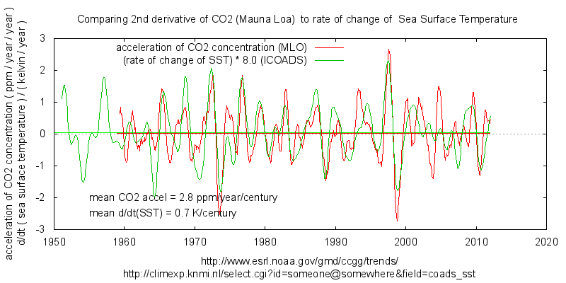
The linear relaxation response that you are using has a frequency dependent amplitude. It will be less for inter-decadal variation that it is for inter-annual variation.
Values for this at two time-scales are estimated from HadSST3 and Mauna Loa CO2 here:
https://climategrog.wordpress.com/?attachment_id=233
Centennial scale will be smaller again, I’d guess about 2 ppm/year/kelvin from those values.
If we takes 0.7K/century rise as the centennial scale temperature variation that gives about 140 ppmv increase due to out-gassing which is about the rise since pre-industrial levels.
Now that 2 ppm/year/kelvin was a pretty crude estimation so maybe we should say 2+/-1 ppm/year/kelvin. It still mean a significant part of CO2 rise could be outgassing.
Mike,
Sorry, but you make the same mistake as Bart: the response of oceans and vegetation to a temperature change is in ppmv/K not ppmv/K/period. A fixed temperature change of the ocean surface gives a fixed CO2 change in the atmosphere, per Henry’s law, no matter if that is static (of a closed sample) or dynamic (all over the ocean ins and outs). It is a transient response at ~16 ppmv/K, not a continuous fixed or accelerating increase in the atmosphere for a fixed temperature step.
I have focused on the simple sinusoids (+ “emissions”), because the theory proves that a linear increase in temperature gives hardly any slope in the derivatives of the transient response of CO2 in oceans and vegetation. If one then applies the same rules to the real temperature data, a slight slope is visible, just enough to match the observed slope of total CO2 rate of change together with the calculated increase rate due to human emissions.
Your 2 ppm/year/kelvin includes both the small rise by the transient response and the rise due to human emissions. In that way, you attribute human emissions to the temperature rise…
What I did show is that the variability is entirely natural and mostly temperature variability induced. The slope of the rise may be temperature induced or human induced, but the latter fits all observations, the former none, except a similar fit of the variability and the slope of the graphs…
So many words, graphs, “conclusions” (convincing only those who make them)…
All this in the face of one undeniable fact: in reality, there was no statistically significant increase in temperature since 1940 if we remove all the falsification (“adjustments”) from the temperature data. Your arguments, gentlemen, are about a wisp of imagination, and play into the hands of the data torturers and ignorant, corrupt politicians.
The following satellite data contained in the document below displays a “pause” in CO2 starting around 2005. Please look at the graph of the ACOS data As supports Dr. David Evans “Notch Theory” research which predicted a decrease in temprature starting around 2005.
http://disc.sci.gsfc.nasa.gov/featured-items/airs_acos_co2_satellite_observations
Figure 6. Time-series of globally averaged CO2 mixing ratios from AIRS Version 5 (2002-2012) and ACOS Version 2.9 (2009-2012). A subset of the ground observations record at Mauna Loa Observatory (1982-2012) (Tans and Keeling, 2012) is given for reference.
Figure 2. The mid-infrared spectrum of clean air in a 24 m cell. Main absorption bands of target gases CO2, carbon monoxide (CO), and water vapor (H2O) are shown. [After Howard (1959) and Goody and Robinson (1951)].
Oddly or paradoxically the reason why there was a 80 ppm to 100 pm drop in atmospheric CO2 during the recent glacial/interglacial cycles is not known. The calculation of CO2 pluses and minuses during the glacial cycle can only account for a lower of 8.5 ppm.
This fact indicates that there are multiple incorrect assumptions concerning the sinks and sources of CO2.
A back of the envelop calculation of the CO2 variance divided by the temperature change for the glacial/interglacial cycle has therefore zero relevance concerning Salby’s assertions.
http://courses.washington.edu/pcc588/readings/Sigman_Boyle-Glacial_CO2_Review-Na00.pdf
“A back of the envelop calculation of the CO2 variance divided by the temperature change for the glacial/interglacial cycle has therefore zero relevance concerning Salby’s assertions.”
Any comparison of what happens during a switch from one quasi-stable climate state to another has no relevance to short term change during stable conditions of an interglacial.
With massive changes to both the biosphere and crypsphere it is foolish to try to infer anything about present variation and causation by looking at de-glaciation transitions.
The ice age glaciations had so much temperature drop that according to the Henry’s Law rules, atmospheric CO2 concentration would have dropped a lot. And glaciations that caused dying-off of vegetation would have trapped some of that dead vegetation under ice/snow, so that would have become CO2 the next time the situation thawed out. From over 400,000 years ago to less than 150 years ago, CO2 did lag temperature by (on average and not constantly) 800 years, while the sum of carbon in the atmosphere, hydrosphere and biosphere was largely constant, and CO2’s role as a greenhouse gas was to contribute to positive feedback of climate changes initiated by other causes. Warmer temperatures caused CO2 to shift to the atmosphere to cause positive feedback for warming, and likewise the inverse for cooling. Within the past 150 years, there has been a new activity of transferring carbon from the lithosphere to the sum of the atmosphere, hydrosphere and biosphere – human combustion of fossil fuels.
William Astley,
“the reason why there was a 80 ppm to 100 pm drop in atmospheric CO2 during the recent glacial/interglacial cycles is not known”
It is not know for certain, but from the papers I’ve read the general opinion among scientists working in the field is that it is due to changes in ocean circulation. There is a constant flux of carbon from the surface ocean to the deep ocean in the form of dead organisms. They decompose in the deep ocean and the CO2 is returned to the surface and atmosphere by upwelling. A reduction in upwelling means less return of CO2, resulting in a drop of atmospheric CO2. There seems to be little, if any, agreement on the cause of changes in ocean circulation.
All these comments prove one thing very clearly….THE SCIENCE IS NOT SETTLED !!!
What is the exact definition of your statement “THE SCIENCE IS NOT SETTLED !!!”?
Nick Stokes:
Hey, if you integrate everything into straight lines; add arbitrary scaling and an offset you can make anything match. That last graph means nothing.
Having filtered out the annual seasonal cycle, it is quite clear from the differential what the relationship is between T and CO2 on an decadal scale. Sadly we don’t have reliable CO2 data back before Keeling started his work, so it’s not possible to accurately scale the relationship on longer time scales but we can estimate it.
Temperature since 1957 is not a straight line so Ferdinand’s attempt to draw conclusions by pretending it is is invalid.
Here is another graph estimating the inter-decadal scaling at about 3 ppm/year/kelvin and clearly showing it to be much stronger on inter-annual scales.
https://climategrog.wordpress.com/?attachment_id=223
Neither temp nor CO2 can be reasonably called a straight line.
In this graph we see, apart from the scaled CO2 / T relationship, a rise of 1 ppm/year around 1960 and twice that now. This could be a response to long term warming, residual anthropogenic emissions or a mixture of both.
I don’t think that there is enough data to extact any more information than that.
Mike,
Where did I use straight lines besides Fig. 3?
I did use several different theoretical variants, including a double sinusoid with and without a slope.
The latter shows that “temperature” and dCO2/dt from a transient response show an exact match in timing and form of the variability. So do the real values. But temperature has a slope and dCO2/dt has no slope in the theory and only a very slight slope in real data.
That means that most of the slope in the real life CO2 rate of change is not caused by temperature but by human emissions…
Here’s another view of the data:
https://climategrog.wordpress.com/?attachment_id=223
Sorry Ferdi, No straight lines anywhere.
Looking forward to Dr. Salby’s reply…
TomRude,
Already waiting over a year to have any of my objections answered…
The increase in CO2 is mostly due to man made emissions. Of course, we are talking about CO2 levels below 1000 PPM and very unlikely to ever exceed that. Such levels are low versus geological history.
The last 500 million years of substantial atmospheric CO2 with no sustained temperature change is compelling evidence CO2 has no effect on climate. This is documented in a peer reviewed paper at Energy & Environment, Volume 26, No. 5, 2015, 841-845 and also in http://agwunveiled.blogspot.com which also discloses the two factors that do cause reported average global temperature change (sunspot number is the only independent variable). The match between calculated and measured is 97% since before 1900.
This is exactly what every popular Internet forum degenerates into as it ages: a posturing ground of a few shrill peacocks proving to each other their obsolete points of view and dressing down anybody who reminds them of reality.
Reality being that nothing, absolutely nothing happened with the climate or with the Earth’s temperature during the last few decades of observation that is not deep within the range of natural variation.
For every single reasonable human being on this planet there are hundreds of Ferdinands and Willises, for whom their little smarting egos are more important than truth, dignity, and anything else. Disgusting.
Amen, alexander, (unfortunately) well said…
Alexander Feht:
For every single reasonable human being on this planet
Where Alexander Feht is the last man standing?
I didn’t say one word about the influence of CO2 on climate and used the satellite temps as most reliable (if not, write your complaints to the RSS people).
Any real scientific objection against what I wrote about the cause of the CO2 increase?
If there is no influence of CO2 on climate, then the whole conversation about it is moot. If there is, your not saying a word about it makes the whole conversation moot.
The discussion/debate on this thread is very interesting. I am exhausted just following it all and will likely return for an encore reading again when time allows.
I hope that this discussion/debate will be recognized by some true unbiased academic professors and will be required reading for their students.
This is WUWT University in action. No other place offers such an exchange of ideas from the level of participants as is being offered here and now! This is absolute brain candy! Please continue.
Thanks to all commenters. And as noted in an earlier comment by Richard Courtney …”Those are three different explanations of alternative possibilities to the narrative you promote and there is not sufficient data to resolve which – if any – of them is correct. …. ”
It’s not quite as simple as we were told by the so-called “climate science” establishment 10 years ago.
The use of Henry’s law in this context is not valid because Henry’s law only refers to the equilibrium between atmospheric CO2 and CO2 dissolved in seawater. However most (ie: about 97%) of the CO2 in seawater is in the form of carbonate and bicarbonate ion. These ions have no impact on Henry’s law at all yet CO2 can migrate rapidly and readily between CO2, HCO3- and CO3= . If the ocean warms and some of the dissolved CO2 goes back into the atmosphere that will increase the pH of the ocean – make it more basic (reduce the carbonic acid level) and the feedback response will be for more carbonate to move to bicarbonate and more bicarbonate to move to dissolved CO2. Thus the 16 ppmv/C is not correct, the sensitivity is actually much higher.
interesting hypothesis. data?
The ocean-atmosphere chemistry is reasonably stable. Climate sensitivity to manmade increase of CO2 is looking low enough for increase of atmospheric CO2 to increase ocean concentration of bicarbonate and H+ ions (slightly reduced pH, slightly more acid). The pH change to less-alkaline is associated with the move to more bicarbonate. Ocean biologists and especially many of the mainstream news media reports of this are concerned with the move to more bicarbonate with decrease of pH being at the expense of carbonate. I have yet to do chemical calculations as for whether the increase of H+ ions outruns the increase of bicarbonate, or the other way around. If bicarbonate increase outruns the H+ ion increase, then carbonate increases, and the opposite means that carbonate decreases – in the likely event I know this chemistry well enough. This is of great concern to calcifying invertebrate animals in the seas, which apparently benefit from carbonate because they build shells that are mainly calcium carbonate.
I am a little curious about calcifying invertebrate animals having any ability to build shells from bicarbonate. It seems to me that the “CO2 alarmists” think that they can’t. Some of them even cite a chemical reaction equation where CO2 + H2O + CaCO3 ==>2*Ca(HCO3)2.
Which is at expense of CaCO3 due to increase of CO2. Yet, I think this is not the whole story. I suspect increased ocean acidity (decreased ocean alkalinity) could have an equilibrium reaction response where the increase of H+ ions is outrun by the increase of bicarbonate ions, which leads to more carbonate rather than less. I invite anyone who can beat me to timely chemical equation work to do so, whether to show more CO2 means more or less carbonate or carbonate staying about the same. I think carbonate would stay about the same or slightly increase as a result of CO2 increase.
Donald,
Some calcifying organisms use bicarbonate as building bloc, incorporating carbonate in their shells and setting CO2 free. See the very interesting Ehux pages at:
http://www.noc.soton.ac.uk/soes/staff/tt/eh/
and the chemistry at:
http://www.noc.soton.ac.uk/soes/staff/tt/eh/biogeochemistry.html
The relative abundance of the three C forms with pH can be seen in the Bjerrum plot:
https://en.wikipedia.org/wiki/Bjerrum_plot
Michael Hammer,
Henry’s law is obeyed in fresh water as good as in seawater, independent of further reactions: it is only for free CO2 (/H2CO3) in water.
A 30% increase in the atmosphere will give a 30% increase in free CO2 as well as in fresh water as in seawater. In fresh water then it stops as free CO2 is ~99% of all C-forms. In seawater free CO2 is only 1% of all C forms, 90% is bicarbonate and 9% is carbonate.
The 30% more free CO2 pushes the equilibrium towards more bicarbonate and carbonate, but also more H+. The latter pushes the equilibrium the other way out. The net result at the new equilibrium is a ~3% increase in DIC (CO2 + bicarbonate + carbonate) in the ocean surface, about 10 times more CO2 absorbed than what was absorbed in fresh water. That is the Revelle factor.
The 16 ppmv/°C is valid, as that is the change in pCO2 – thus free CO2 – per Henry’s law, independent of what the other C species do or don’t. The only difference is that the new dynamic equilibrium between oceans and atmosphere will be reached easier than from fresh water, as the C reserve is much higher.
Ferdinand; below is an essay I wrote some time ago on interactions between CO2 and seawater. Sorry for the length but maybe it is of some interest to some readers.
When CO2 dissolves in fresh water, it forms a weak acid, carbonic acid. So given all the atmospheric CO2 available to dissolve into seawater one might expect that the oceans would be acidic, but they are not, they are alkaline; why is that? How does CO2 interact with sea water and what determines the amount of CO2 the oceans can absorb? Answering these and similar questions is the subject of this essay.
Most gases dissolve to some degree in water. Oxygen dissolved in water allows fish to live. Nitrogen dissolving in water (or blood plasma) can cause the bends in divers. CO2 dissolving in water gives us fizzy drinks and allows oceans plants to photosynthesize. The way gases dissolve in water is described by Henry’s law which states that the concentration of the gas in solution is directly proportional to the partial pressure of the gas above the water. Partial pressure means the pressure exerted by that gas alone, for example if the total air pressure over the ocean is 1 atmosphere and oxygen is 21% of air then the partial pressure of oxygen is 0.21 atmospheres. It means, for example, that doubling the concentration of CO2 in the atmosphere doubles the concentration of dissolved CO2 in the oceans. So does that mean doubling CO2 in the atmosphere doubles the dissolved carbon in the oceans? The relationship might be that simple for oxygen and nitrogen but for CO2 the situation is considerably more complicated.
CO2 dissolved in water undergoes two reversible chemical reactions.
CO2 + H20 = HCO3- + H+ ¬¬ bicarbonate ion plus hydrogen ion (1)
HCO3 = CO3= + H+ carbonate ion plus hydrogen ion (2)
The concentration of hydrogen ions defines acidity. pH is defined as – log [H+] where [H+] means the concentration of hydrogen ions. As [H+] increases, pH reduces, meaning the solution becomes increasingly acidic. Also;
[H+] * [OH- ¬¬] = 1 * 10-14 where OH- is the hydroxyl ion (3)
In pure water [H+] = [OH- ¬¬] = 10-7 which is pH 7 (neutral).
Conversion of dissolved CO2 to bicarbonate ion and carbonate ion generates hydrogen ions, making a solution of CO2 in water acidic. OK but then why are the oceans alkaline? To explain that we need to look at limestone. Limestone is mainly calcium carbonate which is very slightly soluble in water. When it dissolves it splits up into calcium ions and carbonate ions, and the degree of solubility is defined by;
[Ca++ ] * [CO3=] = 4.3 * 10-7 for calcite in seawater (4)
[Ca++ ] * [CO3=] = 6.5 * 10-7 for aragonite in seawater
where as before [Ca++ ] means the concentration of calcium ions. The two common forms for calcium carbonate, calcite and aragonite have slightly different solubilities.
The above reactions are reversible which means they can go with equal ease in either direction. Thus some of the carbonate from the dissolved limestone converts to bicarbonate, thereby reducing the hydrogen ion concentration and thus making the water alkaline. We could also write it as;
CO3= + H2O = HCO3- + OH- ¬¬ and H+ ¬¬+ OH- = H2O
So dissolving limestone makes water alkaline while dissolving CO2 makes it acidic. Pure water in contact with limestone would have a pH of about 10 (quite alkaline), but adding the acidifying impact of CO2 drops the pH to about 8.2 which is roughly the pH of the oceans today.
For these reversible reactions there are always some molecules going each way thereby creating an equilibrium. Chemists have found the equilibrium can be defined by the equations below and equation 3 above;
[H+] * [HCO3-] / [dissolved CO2] = 1.15 * 10-6 (5)
[H+] * [CO3=] / [HCO3-] = 7.41 * 10-10 (6)
The numbers on the right hand side are the equilibrium constants for seawater at 15C, 1 atmosphere. They do change with pressure, temperature and to some extent the presence of other ion species.
Well that’s all very interesting but coming back to Henry’s law, doesn’t it still define the relationship between atmospheric carbon and dissolved carbon? No, it doesn’t, because Henry’s law only defines the equilibrium between atmospheric CO2 and dissolved CO2, the level of bicarbonate and carbonate ion has no bearing on that relationship. Dissolved CO2 that converts to bicarbonate simply reduces the concentration of dissolved CO2 allowing more atmospheric CO2 to dissolve. This ability of dissolved CO2 to convert to bicarbonate and carbonate greatly increases the ability of water to absorb atmospheric CO2.
To see just how significant this effect is, one can calculate the concentration of each species in sea water at an ocean pH of 8.2 and an atmospheric CO2 level of 370 ppm from equations (5) and (6). The relative proportions are approximately CO2=0.5%; HCO3=89%; CO3=10.5%. Most of the inorganic carbon in seawater is in the form of bicarbonate and carbonate. If we increase the amount of CO2 in the atmosphere more dissolves in the ocean and therefore according to equation (5) more tries to convert to bicarbonate. But for every molecule of CO2 that converts to bicarbonate an extra hydrogen ion is produced so [H+] goes up, the pH of the oceans falls and the equilibrium point for bicarbonate and carbonate both move towards a lower proportion relative to dissolved CO2. As pH falls the incremental ocean absorption of CO2 is less than Henry’s law alone would predict.
The above equations define equilibrium levels. If the ocean is not in equilibrium then the equations do not apply and all bets are off. The equilibration between CO2, bicarbonate and carbonate occurs quickly so it is reasonable to assume equilibrium for these processes but is it true for calcium carbonate? After all, the oceans are vast and a lot of the water is nowhere near limestone rock outcrops, so how slow is calcium carbonate equilibration? Well the claim is somewhere between 10,000 and 100,000 years which leads scientists to conclude that over a few decades one can assume essentially no additional calcium carbonate dissolves. Revelle analysed the situation (based on the assumption that there was no incremental source of carbonate or bicarbonate other than dissolving CO2) and showed that indeed as atmospheric CO2 rises, the progressively lower pH means oceans absorb a smaller and smaller fraction of the additional CO2. He defined a Revelle factor = the fractional change in CO2 divided by the fractional change in dissolved inorganic carbon which is claimed to be about 10 on average. Thus doubling atmospheric CO2 only leads to about a 10% increase in total dissolved carbon.
As pH falls, carbonate is progressively converted to bicarbonate (allowing more CO2 to convert to bicarbonate) which, one might assume, would make the oceans under saturated with respect to calcium carbonate allowing the calcium carbonate shells of marine organisms to start dissolving; hence the alarmist prediction that falling pH threatens marine organisms.
This is however not the case. The current [Ca++ ] in surface seawater is reported as 0.01 molar and [CO3=] as 260 micro molar. The product is thus 2.6*10-6 but the solubility product for calcium carbonate in surface water is only 6.5 * 10-7. The surface ocean is significantly supersaturated with calcium carbonate (6 times over saturated with respect to calcite and 4 times over saturated with respect to aragonite). Well if the surface ocean is super saturated, more calcium carbonate won’t be dissolving which supports Revelle’s assumption but it does beg the question as to how it got that way and why the excess calcium carbonate is not precipitating out? The issue is significant because precipitating calcium carbonate would lower ocean pH (by removing carbonate ions) just as dissolving calcium carbonate raises the pH. The answer appears to be that it is stabilised by the presence of organic matter and significant amount of magnesium ions. But how does super saturation come about in the first place? In the deep oceans, additional CO2 is formed by decay of sinking dead animal tissue and excreta and this extra CO2 dissolves due to the pressure just like in a pressurised bottle of soft drink. That reduces both deep ocean pH and carbonate content (reported deep ocean carbonate concentration is around 80 micro moles/liter with pH as low as 7.6). In addition the solubility product for calcium carbonate increases with increasing pressure. The combined impact is to render the deep ocean under saturated with respect to calcium carbonate allowing more to dissolve. As the deep CO2 rich water slowly circulates back to the surface, excess CO2 escapes to the atmosphere, pH and carbonate concentration both increase and the water goes from under saturated to super saturated. This leads to the concept of a calcium compensation depth (CCD), the depth in the ocean where calcium carbonate goes from over saturated to under saturated. Above this depth deposited calcium carbonate shows up in sea floor sediments while below that depth extra calcium carbonate is dissolving and there is no calcium carbonate in the sea floor sediments. http://en.wikipedia.org/wiki/Carbonate_compensation_depth At present the CCD is reportedly between 4000 meters and 5000 meters, well below the level at which shell forming organisms live, but by lowering pH, extra atmospheric CO2 will reduce the level of super saturation (raising the CCD). The impact of various levels of atmospheric CO2 can be calculated from the above equations.
Atmospheric CO2 pH [CO3=]
280 8.3 .000325
370 8.2 0.000271
400 8.17 0.000256
560 8.05 0.000201
800 7.91 0.000152
No one is suggesting atmospheric CO2 will rise to 800 ppm any time soon (the claim has been 560ppm by 2100) but even if it did [Ca++ ] * [CO3=] would be 1.5*10-6 which is still 2.3 to 3.5 times over saturated. It is hard to understand how shell forming organisms can be threatened by dissolution of their calcium carbonate shells when the ocean around them remains significantly super saturated. As with many other CAGW claims, the underlying science may be accurate but the implications of that science are distorted and exaggerated.
There is also another issue of interest. While the high levels of carbonate and bicarbonate in seawater stabilise ocean pH (negative feedback), changing atmospheric CO2 does have some impact. That makes ocean pH a proxy for atmospheric CO2 (along with temperature since the equilibrium constants do change somewhat with temperature). But the claim is that both atmospheric CO2 and temperature have been increasing close to monotonically at least since 1900 so ocean pH should have been falling monotonically since at least 1900. But as Mike Wallace has pointed out (http://joannenova.com.au/2015/01/oceans-not-acidifying-scientists-hid-80-years-of-ph-data/) ocean pH has been measured since 1900 and these measurements show ocean pH has been going up and down between 8.2 and 8 distinctly non monotonically. Does that suggest CO2 should have been going up and down rather than the steady monotonic rise claimed? Well there are wet chemical determinations of CO2 going back as far as the early 19th century and they do indeed suggest exactly that. http://wattsupwiththat.com/2008/07/25/beck-on-co2-oceans-are-the-dominant-co2-store/ Modern climate scientists tend to dismiss as unreliable all the wet chemical measurements that show CO2 levels above 280 ppm but if ocean pH measurements corroborate atmospheric CO2 measurements surely that lends credibility to both. I suspect modern climate scientists probably also dismiss earlier ocean pH measurements preferring modern reconstructions but I see a great danger in ignoring all earlier results that disagree with the latest hypothesis. Those earlier scientists were just as skilled and dedicated as modern scientists albeit working with less well developed, although still adequate, tools. In science generally, earlier work is the foundation on which modern research relies. If that is not the case for climate science we need to have well documented cast iron reasons to justify such a decision. We should remember we are not talking about a single set of measurements carried out by one researcher but rather a large body of results carried out by a large number of researchers which by and large agree with each other. If the earlier results are correct, they speak against the hypothesis that the current rising CO2 levels are entirely due to anthropogenic sources.
Nice, Michael. I will have to study this when I have time.
Michael Hammer:
Your essay is a clear and succinct summary of basic ocean chemistry. I had not seen it before and I have copied it for reference. Thankyou for posting it.
Richard
Michael Hammer in above comment: “… Sorry for the length but maybe it is of some interest to some readers. …”
Thank you for your post. It is certainly of interest to me. I haven’t seen such a well written and easy to follow/understand essay. Seems to be a well written summary of basic ocean chemistry and perhaps should be elevated to a leading post/article. Please consider doing so.
I have read and reread it a couple of times and believe it is much more than “of some interest’ to the readers here. The topic with regards to ocean chemistry is very important.
Michael Hammer,
I do agree with the first part about ocean chemistry… The rest needs some comments:
ocean pH has been measured since 1900 and these measurements show ocean pH has been going up and down between 8.2 and 8 distinctly non monotonically
Before more accurate (colorimetric) pH measurements were used, glass electrodes were used, simply to inaccurate to measure a drop of 0.1 pH unit over 165 years…
Either pH can be calculated from other ocean water observations or in modern times by newer, more accurate measurements. Here for 6 stations over -unfortunately- relative short periods, but they all show similar trends in pH:
http://www.tos.org/oceanography/archive/27-1_bates.pdf
if ocean pH measurements corroborate atmospheric CO2 measurements surely that lends credibility to both.
Forget 99% of the data collected by the old wet chemical methods. Not (only) for their accuracy (+/- 10 ppmv – some much worse) but mainly where was measured: midst of towns, forests (200-300 ppm diurnal change),… The historical data taken on board of ships and coastal with wind from the seaside all were around the ice core data for the same period. See further:
http://www.ferdinand-engelbeen.be/klimaat/beck_data.html
Hammer +1000
Yes dress this up and make it a separate thread here. One thing I noted is the higher solubility of aragonite and I immediately understood how these cunning shellfish can make conches even with some increase in pH that dissolves more calcite. It never ceases to amaze me how nature constantly instructs us not to be linear thinkers (to little avail it seems)
Bravo.
Worthy of elevation to a permanent sticky note. But that’s not likely, is it.
It’s the oceans!
Ice core analysis repeatedly show that CO2 increases lag Earth’s temperature increases about 200 years. CO2 concentration began increasing about 65 years ago. LIA low point was about 1750, or 265 years ago. Just like the ice cores indicated it repeatedly happened long before humans were a significant source of atmospheric CO2. KISS!
QED!
Thanks for this post – well done and informative.
The following phrasing had me wondering about history.
“Human emissions show a slightly quadratic increase over the past 115 years.
The “115” years does not go even halfway to early industrial processes and major CO2 production. I was recently reading about early steel-making in Western Pennsylvania (my home region). About 1860, ovens began to replace mounds but the beehive ovens released all the gases and other waste during coking. The number of beehive ovens between 1870 and 1905 grew from about 200 to almost 31,000 and peaked in 1910 at almost 48,000. A newer, much larger “by-product” oven, captured the chemicals as uses were being found for them.
Historical info: {enlarge the lithographs}
http://explorepahistory.com/hmarker.php?markerId=1-A-2C3
Modern photo:
http://cdn1.vtourist.com/4/4562757-Coke_ovens_Connellsville.jpg
John F. Hultquist,
Thanks for your comment…
Before 1900, yearly human emissions still were largely within the noise of the year by year variability, although the trend was already emerging from the variability. After that the trends of both human emissions and CO2 increase in the atmosphere get clearly out of the noise…
Coralline sponges give already a clear change in 13C/12C ratio from 1850 on, due to the emissions of low-13C from fossil fuels and radiocarbon dating needed correction tables from 1870 on because of the zero-14C addition by humans…
“– The temperature-only match violates all known observations, not at least Henry’s law for the solubility of CO2 in seawater, the oxygen balance ”
I’ve lost my link to a paper with estimates of the equilibrium constants as a function of temperature in saline solutions. I do remember that K1 decreased with temperature in the range 20-30°C. I could be wrong.
Do you have a link to this or similar work?
And being pedantic, Figure 15 (and possibly others) has T-anomaly °C/month.factor+offset for y axis when the its not the derivative.
Robert B,
http://www-naweb.iaea.org/napc/ih/documents/global_cycle/vol%20I/cht_i_09.pdf
contains at page 7 tables for the different dissociation constants for different temperatures and salinity and graphs at the next page…
BTW, thanks for spotting the error…
You are pretty sure ? that tells me all I need to know about your science … I’m pretty sure you are wasting our time …
You have no idea what global temperature is doing ass your figures 14 and 15 show. You cannot draw a a straight line through these data sets. The super El Nino in the middle separates the data into two segments, differing by a step increase of a third of a degree just after its departure. Both the right side and the left side of the temperature curve are each represented by a horizontal straight line, each designating the existence of a sepasrate hiatus. You just may have heard that the existence of a hiatus nullifies the greenhouse theory of global warming. It is not for nothing that Karl thinks his paper is a “pause-buster.” That is fakery, obtained by changing temperature curves retroactively. The U.S. Congress wants to know about it but NOAA has refused to give any info. As to the slope of the carbon dioxide curve, who cares. Having a hiatus proves it does not warm. Just look around . Have you noticed that CO2 has been increasing for 18 years without causing any warming?
arnoarrak,
I did only use the trend lines to align the temperature trend (as Bartemis insists that is the only cause of the CO2 increase) with the CO2 rate of change trend. The human emissions + natural variability did fit the slope perfectly.
My only aim was to show that human emissions are the cause of the CO2 increase in the atmosphere not temperature, as many skeptics still think.
That has no effect on better arguments to counter the warmistas: that the models are way too high today in their “projections” and indeed no temperature increase for a record CO2 level…
I see this argument continuing for a very long time. Here is what is known,CO2 is increasing, CO2 can cause warming. What is not known is what are the sources and what each contribute to the additional CO2. Next how much warming will come from the additional CO2. Present projection are somewhere around 1.5 degrees which if true make the entire debate moot. I will also inject we do not at this point and time know if the warming of land base temperature, is a measurement, adjustment or siting artifact. I do know no definitive statement about anything in climate should be take seriously since it quite simply the science is to young there are too many variables to know whether the temperature is actual rising now and at what rate. The best measurement we have are satellites and their measurement period is to short to tell us anything. Argo is a bucket of spit it is so full of variables there is nothing there, on top of the their deployment is of such a short of time and trends are to short to be any value.
This leave us too reason entire climate change, CGW debate is only about one thing it control, their a group of people that think they know all the answers and want to tell the rest of us peons what to do. There is one definitive answer on that is, when the elites come down from the mountain with all the answer they are always wrong and millions will die because of it. That is not a world I want to have to live in, nor should it be for anyone else. Let us learn fine some light walk slow with the light and do not run into the darkness, because someone or some group said it was safe. For god sake let make sure their so call cliff we are trying to not drop off of is indeed cliff no a small drop that we can simple step over. After the climate debate is still has us in a deep fog uncertainty and we do not know what is in front and what was behind us since most of us did not look back at the time we traversed the climate terrain.
Cutting back on fossil fuels may be like climbing a mountain easier to climb up than it is to climb down and the worst part of that we are doing it in a fog, we don know if we are on summit, a ledge of it we are hanging off the ledge all and honest person can say is I don’t know what the best route. This best thing is to proceed with caution and try to learn the terrain as much as possible and for god sake don’t get up and run any direction because some one or some group yelled fire. Especially when it might be someone’s camp fire and they are just trying to stay warm.
AGW debate is just like the middle age debate of “How many angels can be on the point of a pin” pure sophistry , it does not matter a huge waste of time. It looking more and more AGW reality is it does not matter it is sophistry a waste of time and money. I would not bother to pay attention to it but the AGW crowd has crawled into my wallet and are causing everything I do to be more expensive from what I can see is very little evidence or reason. Climate research is not a waste of money but making grand statement from that research is sophomoric. I do believe generation to come are going to be asking who stupid where these people to believe man could greatly affect climate at the 21 century level of technology.
It can be boiled down to the lack of tropospheric hotspot which outright disproves the positive feedback hypothesis. Combined with the ERBE satellite measurements that show OLR goes up with surface warming not down and global temperatures are a third of the GCMs it shows the Climate sensitivity parameter is far less than the alarmists project, meaning there’s no crisis and no proof that a warm climate is bad at all anyway.
i challenge anyone to provide a shred of proof to the contrary.
http://papers.ssrn.com/sol3/papers.cfm?abstract_id=2642639
+10
Chaam Jamal,
Have you really read that abstract?
A statistically significant correlation between annual anthropogenic CO2 emissions and the annual rate of accumulation of CO2 in the atmosphere over a 53-year sample period from 1959-2011 is likely to be spurious because it vanishes when the two series are detrended
When you detrend the two series, you effectively remove the influence of human emissions (which are all trend and little variability) and the remainder is the variability caused by temperature (which is all variability and little trend). Quite obvious that the conclusion is that there is no correlation between CO2 emissions and detrended CO2 rate of change…
Errr, excuse me for stating the obvious, but is there not a much easier way of demonstrating and proving this??
If we look at the Ice Age record, we see that for a 10 degree warming, we get a 100 ppm CO2 increase. Or 10 ppm per degree of warming. So if we have warmed by 2 degrees in recent decades, the natural oceanic CO2 increase will be 20 ppm. And anything in excess of this must be anthropogenic.
QED. This is not exactly rocket science.
.
http://www.brighton73.freeserve.co.uk/gw/paleo/400000yearslarge.gif
“…not rocket science”
Ralfellis, no but it is climate science. (at least with a rocket you can verify if you are wrong) Ice cores are unverified. They can be smoothed or co2 can get lost in the upper parts of the core as time goes by. As well, fewer trees are around during an ice age thus less sequestration of co2. As well, what role does a longer time period play in the stabilization of co2 levels (as recent warming has been relatively fast). So the “obvious” may not be so obvious after all…
Fonzie,
Except that the 8-16 ppmv/°C is in the ballpark of Henry’s law: 4-17 ppmv/°C in the literature for the solubility of CO2 in seawater…
Ice cores are unverified? Every new technique is “unverified” as the older techniques were by far less accurate… That was the case for CO2 measurements: the NDIR method used by Keeling Sr. was “unverified”, as its accuracy is better than 0.1 ppmv, while the old chemical methods were accurate to +/- 10 ppmv…
There is an overlap of ~20 years (1960-1980) between two Law Dome ice cores and direct measurements at the South Pole, overlapping ice cores with different resolution, different temperature, different snow accumulation rate, each showing the same CO2 levels +/- 2.5 ppmv for the same averaged gas age…
Ferdinand, it’s one thing for co2 to be sitting around in ice for twenty years, quite another for it to be sitting around for thousands of years. BTW the neftel numbers at your site show 3ppm lower than MLO when overlapping. I was also wondering why they use two different cores to demonstrate the overlap at law dome. Less than a decade worth from the very upper most part of the two cores may not tell us much about smoothing/co2 loss…
Fonzie,
They drilled three cores at Law Dome, to test the influence of different drilling techniques on the CO2 record (wet and dry).That was one of the many objections the late Dr. Jaworowski had against ice cores… Two were at the summit, going back 150 years in time. The third was downslope with thinner layers, allowing a view of 1,000 years back in time…
The overlap of ~20 years shows that at the start of full closure, ice bubbles and atmosphere are equal, thus no selective discrimination for CO2…
3 ppmv may be the difference between Mauna Loa and South Pole CO2 in 1960-1980, need to check dat…
Ferdinand, i see bart has chimed in at the bottom of the page. This could get interesting (have fun…). Let me clarify; to show that ice cores match atmospheric concentrations they use both DE08 (’62-’69) and DE08-2 (’70-’78). This is good for demonstrating that the age of the air is the same as the atmosphere, but not so good if we want to see some smoothing. Using just the very top 7 or 8 years of each of the two cores is not going to show us much in that regard… Just eye balling it, it looks like SP is just 1 ppm lower than MLO. So the neftel data shows 2ppm less than SP. (But, it looks like they simply matched the top of the siple curve to the MLO data anyway at 328 ppm in ’73, no?)
One other tidbit i’d like to put out here; in the deeper cores, closing time on the bubbles is as much as 600 years (?). (it’s been said that a spike like the present one won’t even show up with averaging like that) THUS, the henry’s law ratio of co2 to temperature may be underrepresented in the deeper (low resolution) cores…
Fonzie,
The current spike of 110 ppmv in 165 years would be visible in all ice cores, be it with a lower amplitude thanks to the lower resolution…
.
Ferdinand — so what do you say to my quick and simple empirical calculation? Your complex calculations suggested 16 ppm per degree centigrade. My simple calculation based on data going back 500,000 years suggests 10 ppm per degree centigrade.
So we are in agreement, yes?
Ralph
ralfellis,
We are largely in agreement…
But there is one correction needed: the temperature proxies (dD and d18O of the ice) show the temperature changes at the place where the snow was formed, thus somewhere around Antarctica. The warming and cooling episodes are a lot larger in the polar areas than around the tropics, thus the global change is about half the polar change or a near doubling of the CO2/temperature ratio…
But don’t worry, I have used a lower ratio for years, doesn’t matter much, what matters is that there is a rather fixed ratio between temperature changes and CO2 changes and very little effect in the reverse…
Point taken.
In which case, my empirical calculation shows a 20 ppm increase per degree centigrade of warming on a worldwide basis. While your methodology shows 16 ppm per degree.
Ralph
ralfellis:
Indeed, it’s not rocket science that there’s ~10ppmv overall change in CO2 per degree Celsius evident in the Vostok record. The rub comes in the fact that these are Antarctic temperature changes compared to quasi-global concentrations of a well-mixed gas. Furthermore, that’s insufficient scientific basis for attributing causality to temperature without additional analysis.
In principle, both variables can be driven by another variable (say, global insolation) with starkly different response characteristics, resulting in concomitant behavior. Add a strong new (anthropogenic) source of CO2 in the 20th century and the highly muddled claim of causality for CO2 arises, despite cross-spectral evidence that it either lags temperature (lowest frequencies) or is incoherent with it (highest frequencies).
Ralf,
Sorry, but it is not that simple. Among other reasons, consider that there are more carbon sinks during interglacials than glacials.
Just as there is not a single equilibrium climate sensitivity to CO2, the amount of CO2 in the air is also not strictly a function of temperature, although perhaps given enough time, it might be. But there is rarely if ever enough time.
After the ice sheets melt under warmer conditions, then land plants spread, drawing down CO2. But T can remain high during deglaciation while there are as yet enough sinks to bring CO2 back into line.
But IMO, it doesn’t matter much whether the 120 ppm of CO2 allegedly added over the past 160 years is mainly man-made or not, since the increase has negligible effect on climate, but an obvious beneficial effect on vegetation.
This argument about expecting 1 degree from 10ppm comes from the hypothesis that CO2 is a driver of global temperature in the first place; ie it is a circular argument.
If the Antarctic is such a good proxy for the globe then why is it cooling and expanding now contrary to expectations? The usual answer from climate scientists to the odd cooling is that it has a unique climate system.
There are other proxies which contradict the lock-stepness of the Antarctic ice cores between CO2 and temperature – Arctic ice cores, geological data and plant stomata recons. So you have to ignore alternative data and the uniquess of the Antarctic to be able to imply that CO2 is a climate driver.
An alternative and more plausible explanation which is borne out by all other observations and the failures of the models to predict a pause is that CO2 is not a climate driver – rather just a weak feedback to rising temps that arise from another cause, ie the sun. QED. It isn’t rocket science but it isn’t about cherry-picking either.
This argument about expecting 1 degree from 10ppm comes from the hypothesis that CO2 is a driver of global temperature in the first place; ie it is a circular argument.
________________________________
All you have to do is reverse your statement. In reality 10 ppm comes from 1 degree of warming. Now everything is correct.
See my post and graph directly above.
Ralph
JasG,
Ralfellis is correct: in ice cores, CO2 follows temperature with a lag, without a sign of the opposite. Thus temperature increase causes CO2 increase.
Further, ice cores are accurate direct measurements of CO2 (and other gases) in ancient air, be it a mixture of 10-600 years, depending of the snow accumulation rate. The rest are proxies, with all the problems they have: stomata data need to be calibrated to ice core CO2 for local bias, geo data are much too coarse and ice cores from Greenland are unreliable for CO2 because of frequent deposits of highly acidic ash from Icelandic volcanoes, which react with sea carbonate deposits to form in situ CO2…
This whole discussion is spurious because the planet’s major CO2 producer has been ignored. VOLCANOES: these produce not only tonnes of CO2 but also HCl, H2S, SO2, HF,HCN into both oceans and atmosphere. Remember there are more volcanoes below the ocean’s surface than those of continental origin. Volcanogenic CO2 isotope ratio is identical to that of burning fossil fuels. So where does the CO2 originate? Certainly not humans trying to live a good life.
In addition, take earth quakes as indicator for tectonic activity
http://research.dlindquist.com/quake/historical/?mag=0&type=num&freq=year&style=raw
The number of all quake rose 6 fold from 1973 to 2008.
Looks like a Hockey Schtick by the way.
johnmarshall,
Measurments around active volcanoes (mount Etna, Sicily/Italy) show that volcanoes emit ~1% of human emissions. Undersea volcanoes emit within the huge ocean reservoir. Volcanic CO2 isotope ratio is way higher in δ13C than fossil CO2: around zero per mil for subduction volcanoes, around -6 per mil for deep magma volcanoes. Human emissions are around -24 per mil…
Thus yes, humans are the cause of most of the increase…
No one, even IPCC, knows what’s happening on the ocean floor.
Ferdinand E.:-
Total rubbish, You need to look at the data not wishful thinking. Volcanogenic CO2 has been the major input for 4.6Ga. Human input can be ignored.
Nicholas, what happens at the ocean floor largely stays in the deep oceans, except maybe in the Bermuda triangle if the stories are right…
John Marshall: besides the Decan and Siberian traps and a few large meteor impacts, the release per unit of time was minimal. Even the largest volcanic event of the past decade: the Pinatubo, larger than all eruptions of the past century together, caused a drop in the CO2 rate of change…
Ferdinand,
So you think that, without the human CO2 emissions, atmospheric CO2 would not be increasing (zero or very small trend), something like this (but at the lower “preindustrial” level of 280 ppm?):
http://www.woodfortrees.org/plot/esrl-co2/plot/esrl-co2/detrend:82
edimbukvarevic
Slightly more upward: without human emissions, CO2 levels follow the temperature trend at ~16 ppmv/°C. You can better plot the temperature anomaly with a factor 16 to see what happens with CO2 from natural sources…
Obviously, there are a number of superficially attraction to the argument that human emissions are solely or mainly responsible for the observed rise in atmospheric CO2 since the mid 19th century, not least that manmade emissions are a new source of CO2, that came into existence at around that time, and that the rise in atmospheric CO2 is coincident in time upon manmade emissions.
Obviously, it is superficially attractive to suggest that if man was not emitting any CO2, then the total sources, whatever they are (and there is significant uncertainty with respect to them), would be less such that less CO2 would be being emitted into the atmosphere, from which it should follow that the amount of atmospheric CO2 in the atmosphere similarly be would be less.
On a related argument, obviously it is superficially attractive to argue that whatever the size of the carbon sink is today and however it is constituted (the fine detail of which are not known, but do not need to be known), it is greater in size than the cumulative value of sources, whatever these be including that of human emissions (again we do not need to know the precise detail but merely the relative size of the sinks verses sources), such that if we were to reduce (or eliminate) human sourced CO2 emissions, the amount of atmospheric CO2 would fall.
But underpinning all these superficially attractive propositions are a number of assumptions, the validity of which is uncertain. I set out a few of these, but not an exhaustive list.
First, the assumption that we know sufficient about pre 1959 Mauna Loa atmospheric conditions. Ferdinand does not, in this post, deal with the Beck reconstruction. Ferdinand considers that the Beck reconstructions can be dismissed because Mauna Loa (and other observations that match it fairly well) deal with high altitude CO2 and at high altitude CO2 is a well mixed gas, whereas the Beck data pertains to ground sourced samples whereat CO2 is not well mixed and is in fact highly variable such that that data set cannot elucidate what the global high altitude CO2 composition was at the relevant time.
Now whilst the point raised by Ferdinand for dismissing the Beck data may be sound, I consider that it points to a problem, namely that the source and sink interchange is not taking place at high altitude where the Mauna Loa CO2 data is being measured but rather at the surface, where we do not know what changes if any with respect to the concentration of CO2 has taken place these past 150 or so years.
Ferdinand relies upon the fairly steady and monotonic increase in CO2 (as measured by Mauna Loa), but since the source and sink interface is essentially at ground level there may be many more complexities happening at ground level that we do not know about, and which may more accurately explain the incessant rise in CO2 at high altitude which rise is at a rate less than the anthropogenic emissions of CO2.
Second, Ferdinand relies upon Henry’s law, but there are a number of problems with this namely that the oceans are dynamic, the chemical composition of which is in flux (not simply dissolved CO2), and they are not a system in equilibrium. I consider that issues arise when one makes an assessment on the basis of average temperature when in practice the oceans extend over a vast area and have a substantially different temperature across that area ranging from around 2degC (the Polar oceans ) to 34degC (Red Sea, Gulf of Mexico, Some areas of the Indian Ocean, South China Seas etc). There is also a diurnal difference in the temperature of the oceans, more pronounced depending upon ocean basin and latitude, and prevailing currents. The outgassing and the sequestering of CO2 is different and CO2 outgassed in one area is not necessarily sequestered back in the same area, so it becomes much more difficult to apply Henry’s law.
Third, there seems strong evidence that CO2 lags temperatures by about 600 to 1000 years. The rise in CO2 that we are seeing today may simply be a response to the temperature change that took place in the MWP, and it is just coincident that today there is late 19th century and 20th century industrialisation of the planet leading to anthropogenic emissions and perhaps further coincidence that the late 20th century warming is broadly similar to that which took place in the MWP.
My view is that without getting on top of the sources and sinks, by which I mean identifying each every source and each and every sink, and precisely how much CO2 it is sourcing, or sinking, as the case may be, we do not know whether the position put forward by Ferdinand is correct. Presently, there is simply too much uncertainty surrounding sources and sinks (we keep on discovering more of them) and too much uncertainty surrounding the estimates that we have placed upon them in the carbon cycle.
I consider that this exposition by Ferdinand is useful, and helps us gain insight into the Carbon Cycle, but like too many areas in this ‘science’ there is a lack of knowledge, insufficient or poor quality data, which results in our lacking the necessary understanding of the processes involved.
Richard Verney,
It wonders me every time again, that some skeptics are rightly pointing to the lack of quality in temperature measurements, but do like the compilation of the late Ernst Beck as the truth. Beck’s data are a mix of the good, the bad and the ugliest CO2 data one can imagine. All lumped together in one compilation.
It is comparable to one year of temperature measurements in Oslo, Norway at a good situated site, followed by a year of data in Rome on an asphalted parking lot and later back to a year in Moscow. The conclusion: the middle year shows a peak in temperature…
That is the quality of Beck’s compilation. Thus sorry, that is no argument at all. See:
http://www.ferdinand-engelbeen.be/klimaat/beck_data.html
We have ice cores which show filtered values of various resolution: over the past 150 years with 10 year resolution, over the past 1,000 years with 20 years resolution. More than sufficient to see the evolution of CO2, CH4, N2O, CFC’s, 14C bomb spike,… in the atmosphere. Including a 20 year overlap (1960-1980) with direct measurements at the South Pole.
If we take the historic CO2 measurements which were taken over the oceans or coastal with wind from the sea side, the values are around the ice core levels for the same period…
CO2 levels at Mauna Loa at 3,400 m height are near identical to those taken at Cape Kumakahi at 3 masl. CO2 levels in 95% of the atmosphere from near the North Pole to the South Pole show yearly average CO2 levels differing less than 5 ppmv, mainly due to the NH-SH lag…
Ferdinand relies upon Henry’s law, but there are a number of problems with this namely that the oceans are dynamic
While there are a lot of ingoing and outgoing fluxes, they all obey Henry’s law. That makes that any increase in temperature increases the local ocean pCO2 with 16 μatm/°C. For the sources that means an increase in CO2 release. For the sinks, that means a decrease in sink flux. The net result is an increase of the CO2 level (pCO2) in the atmosphere. When that reaches ~16 ppmv/°C, the original in/out fluxes are restored.
The net result of a dynamic equilibrium for the whole ocean surface or for a static sample are exactly the same for the same change in temperature…
Third, there seems strong evidence that CO2 lags temperatures by about 600 to 1000 years.
That is for deep ocean temperature changes which need 5,000 years to warm up. The MWP-LIA cooling of ~0.8°C (depending of the reconstruction), did give a drop of ~6 ppmv with a lag of ~50 years after the temperature drop. A similar increase in temperature since the LIA thus is good for 6 ppmv?
What you miss in this debate is that more and more is known about the individual fluxes, but that the main balance is quite accurately known: human emissions, increase in the atmosphere and net sink rate. Plus a lot of other observations: 13C/12C ratio, 14C decline, oxygen balance, process characteristics,… which all point in one direction: human emissions as cause of the increase…
Ferdinand
Your answers do not seem to address the fundamentals behind the points that I raise. For example,
You state:
It wonders me every time again, that some skeptics are rightly pointing to the lack of quality in temperature measurements, but do like the compilation of the late Ernst Beck as the truth. Beck’s data are a mix of the good, the bad and the ugliest CO2 data one can imagine
Implying that I accept the Beck data as being valid, but you overlook that I specifically stated:
Now whilst the point raised by Ferdinand for dismissing the Beck data may be sound
You say:
Beck’s data are a mix of the good, the bad and the ugliest CO2 data one can imagine
And this is not because there is any problem with the equipment used for testing, nor the manner in which the tests were carried out, but rather because of the sampling itself. The sampling was from areas where CO2 varies significantly from hour to hour, from day to day etc. We have had several exchanges over the last few months on this, and you have provided independent evidence that CO2 is not a well mixed gas at low altitudes, and it this fact that causes the Beck data to be the bad and ugly.
You fail to address in your reply, the implications that follow from the fact that CO2 is not well mixed at low altitude and is extremely variable and the relevance of this fact, on the sink and source interface.
I do not consider that you have given sufficient thought to the issue regarding average ocean temperature and that CO2 outgassed in one area may be carried with winds to another area where the ocean temperature is significantly different. Those winds are never constant, and the places to where CO2 may be swept is continually changing. I consider that you need to give further consideration to the problems created by dealing with everything on an average basis when in fact it is highly variable certainly in 2 dimensions and possibly 3 dimensions. Perhaps OCO-2 will, in time, shed more light on this.
The thermohaline circulation is considered to be in the order of a 1000 years. Wikipedia states:
If it is 5,000 years, as you suggest, we are going back to the time of the Old Kingdom (In Egypt) which was another warm period. So the same problem emerges.
If there are wide estimates as to capacity of each of the individual sinks (as there is) and if there are wide estimates of the individual sources (as there is), and if we are still finding new sinks and sources (which we are), it is wishful think to conclude
The point I make is that we do not know enough about this as your own reply demonstrates.
Whilst I have not yet studied this, I presume that you have looked at (or will be looking at):-
http://wattsupwiththat.com/2015/11/26/report-global-growth-in-co2-emissions-stagnates/
There are several strange steps in the Mauna Loa data series, not simply those identified in the above article, which do not fit particularly well with your view of the Carbon Cycle and the rise in atmospheric CO2 levels.
Personally, I am not greatly concerned by all of this since the fundamental issue is not why CO2 may be rising (although if this is not because of anthropogenic actions, a policy of mitigation is worthless and will fail to curb emissions), but whether it is significant. In other words, what is Climate Sensitivity (if any at all) to CO2. This can only be answered by observational evidence, and hence I am much more concerned at getting good quality observational data that will elucidate that.
The reason behind the rise in CO2 seems very much a secondary issue especially since the globe is presently starved of CO2 so rising CO2 would appear to be a welcomed event. If it brings some warming with it, so much the better because the globe is also rather cool and in the round all life would benefit from a warmer biosphere.
Richard Verney,
The ugly data were from equipment not suitable to detect atmospheric change to any reasonable accuracy:
– That was the case in Barrow: equipment used to measure CO2 in exhaled air (20,000-40,000 ppmv!) was calibrated to outside air. If that was between 200-500 ppmv, the equipment was ready to use. Accuracy +/- 150 ppmv…
– That was the case in Antarctica: equipment accurate to +/- 200 ppmv. O2 measurements down 2% in some samples, CO2 elevated to over 1000 ppmv in some samples…
– Thousands of seawater samples at 0 m depth were catalogued as air samples, while the pH of the samples was measured…
After long discussions, Beck dropped the first two as unreliable, but never admitted his error in the last one.
Then we have the bad ones: that are all data taken on land, except in deserts or on mountain tops, far from vegetation, as that is the main cause of the variability. The variability is far less over the oceans: maximum 10 ppmv between North Pole and South Pole, including the large seasonal variability and the NH-SH lag. That is in 95% of the atmosphere…
The variability over the oceans has hardly any influence on yearly average uptake and release. The variability over land is the result of the uptake and release by the biosphere. But that all doesn’t matter: we know the net result at the end of the year, for every year of the past 55+ years with reasonable accuracy…
Further:
The THC needs ~1000 years to return from the polar waters to the equator, but the warming of the full deep oceans needed 5,000 years.
Even the 1,000 years has little effect: the MWP may have had 10 ppmv more CO2 in the atmosphere than today, that results in maximum 5 ppmv more in the current atmosphere, not 110…
Where we agree is that the increase of CO2, whatever the cause, will have little effect on temperature/climate…
November 26, 2015 at 4:53 am
I posted this above:
co2 and o2 rise and fall in step (anti phase) the yearly cycle is mainly plant respiration (O2 out in light ; co2 out in dark). If this is the case then the respiration is from land plants / sea phytoplankton outside the tropics, It is not from growth and decay since decay is too slow to give the rapid increase in co2 in NH autumn – when temperatures fall decay rate is low.
a plot of CO2 and O2 is here:
If CO2 in ocean solution was cause of dips and slopes then O2 would not be inverse.
-=-=-=-=-=-=-=-=-
Additionally.
Any CO2 eruptions from volcanic activity, or CO2 release from sea water solution would produce a rise in CO2 without a corresponding fall in O2 the plot clearly shows rise in co2 and simultaneously a fall in o2 – i.e. the carbon is being oxidised to Co2. and a fall in CO2 has a corresponding rise in O2 – i.e. the CO2 is being reduced to C + O2
http://4.bp.blogspot.com/-bCvtAJzSBMY/T9ptnRzSP9I/AAAAAAAAAYc/1NYuolWUs_w/s1600/co2+-+02+all.jpg
Thank you for this very thorough analysis Ferdinand. You cover one of the most fundamental issues in climate science and your analysis is extraordinary convincing.
Let me just add that the Vostok ice core shows that the CO2 level has not been above 300 ppm in the last 800 000 years.
http://cdiac.ornl.gov/trends/co2/ice_core_co2.html
I think this data series alone is evidence enough to conclude that the current level of 400 ppm is caused by humans.
I wonder whether those who object to that think that the current CO2 level is just natural variability, and that it is just a coincidence that it happens now, and never before in the last 800 000 years, or do they think that the Vostok ice core is bogus?
/Jan
Ice cores are the tea leaves of climate science, an entertaining parlor game, but too much uncertainty and co-confounders for scientific value.
If ice cores are tea leaves, then what are stripbark pines?
And yet temperatures have varied quite a bit during that time. Much more so than can be explained by a change of just ~30ppm of CO2. WUWT?
No Richard, they match very well with theory,
As Willis describes above, the relation between temperatures and CO2 in Vostok gives us a value of a change in CO2 due to temperature rise of ~ 16.5 ppmv/°C, in very good agreement with Henry’s Law.
This must of course not be confused with climate sensitivity, which is the opposite effect, i.e. the change in temperature caused by change in CO2. The climate sensitivity is in the range 1.5 to 4.5 °C for a doubling of CO2.
Both climate sensitivity and Henry’s law are real physical phenomenon and Henry’s law is one of the positive feedbacks to the climate sensitivity.
/Jan
Over the last 800,000 years temperatures have varied by approximately 13 to 14degC, and during the same period CO2 has varied by about 100ppm (from about 200 to ~300ppm). See, eg the right hand plot:
http://lafenergy.org/essays/gwfig1.php
It is difficult to see how that is in good agreement with Henry’s law, and it is nothing like ~ 16.5 ppmv/°C, but rather much more like ~7.5 ppmv/°C (ie., 100ppm/13degC).
Over the last 2000 years (before say 1800 AD) there has been all but no increase in CO2 and yet we have seen the Roman Warm Period, the Medieval Warm Period and the LIA.
See the top plot at:
http://cdiac.ornl.gov/images/three_gases_historical.jpg
Richard,
You cannot just take the maximum difference in CO2 and divide it by the maximum difference in temperatures, and think that you get the relation between CO2 and temperature from that.
That will only work if there is a 100% correlation between the two, but it is not.
The correct way to identify the relationship between the two is to make a scatter plot with CO2 and temperatures.
This is done in figure 1 in
S. Torn, Harte, GEOPHYSICAL RESEARCH LETTERS, VOL. 33, L10703
The relationship found is 14.6 ppm/C
/Jan
Richard Verney,
You need to take into account that the dD and d18O temperature proxies in ice are mainly from where the snow was formed, thus in near polar areas. The temperature change there is about twice that of the global temperature change. Thus you need to increase your polar ratio to have the global ratio…
Good point Ferdinand,
however, the figures I provided of 14.6 ppmv /°C was from the average Southern hemisphere, not the local Vostok temperature.
The Torn and Harte paper says:
Furthermore:
I cannot see that the paper Richard provided specify whether they use local or temperatures or not.
/Jan
Thanks Jan,
Not far off the 16 ppmv/°C that Henry’s law gives for seawater pCO2 change. I can live with that difference…
Hard to use that for the 110 ppmv CO2 increase over the past 165 years. Boiling oceans somewhere?
Boiling oceans, nobody has ever seen a storm at sea. That would have to reduce the pressure over a very wide area. I’m sure that only water vapor is the only gas that is being released as if that could happen. When I release the pressure on a bottle of soda/pop it never fizzles either. Or goes flat.
rishrac,
Have been sailor (engine room) myself some (very) long time ago, still remember a few severe storms… But was just joking about boiling oceans. With a severe storm, the mixing between oceans and atmosphere is certainly very intense and a lot of CO2 and water vapor released into the atmosphere from warm oceans. Once mixed in the bulk of the atmosphere, I don’t think that will give much difference in CO2 levels, or one should see that in temporarily higher levels after major hurricanes…
A very long analysis to state the obvious: if the atmospheric CO2 concentration rise would not be caused by the emissions from burning fossil fuels, where then would have gone the 385 Pg carbon emitted since the beginning of the industrial era, or the current 10 Pg C per year ?
It can’t jump from a flame to be immediately sequestered by biomass or the seas, it has to stay in a certain quantity in the atmosphere (in fact 50-60%) for a while.
Other point: if CO2 absorption in sea water would only be driven by Henry’s law, then only a minuscule amount would be absorbed. The actual driver is the carbonate formation, a chemical reaction between water and the weak acid CO2.
All hart analysis without stating the corresponding coefficient of correlation is as valid as stock market chart analysis. In fact no statistically valid correlation can be established between T and CO2.
See https://hal.archives-ouvertes.fr/hal-01146608v3/document
Ferdinand Engelbeen:
Thanks for the post. An interesting thread. I appreciate your effort in clearing up the comments, as well.
Ferdinand
Further to your comment Ferdinand Engelbeen November 26, 2015 at 8:27 am
Your answers do not seem to address the fundamentals behind the points that I raise. For example,
You state:
Implying that I accept the Beck data as being valid, but you overlook that I specifically stated:
You say:
And this is not because there is any problem with the equipment used for testing, nor the manner in which the tests were carried out, but rather because of the sampling itself. The sampling was from areas where CO2 varies significantly from hour to hour, from day to day etc. We have had several exchanges over the last few months on this, and you have provided independent evidence that CO2 is not a well mixed gas at low altitudes, and it this fact that causes the Beck data to be the bad and ugly. In your response to me, you do not seek to argue that CO2 is well mixed at low altitudes or that I am incorrect in pointing out that CO2 is not well mixed at low altitudes.
You fail to address in your reply, the implications that follow from the fact that CO2 is not well mixed at low altitude and is extremely variable and the relevance of this fact, on the sink and source interface.
I do not consider that you have given sufficient thought to the issue regarding average ocean temperature and that CO2 outgassed in one area may be carried with winds to another area where the ocean temperature is significantly different. Those winds are never constant, and the places to where CO2 may be swept is continually changing. I consider that you need to give further consideration to the problems created by dealing with everything on an average basis when in fact it is highly variable certainly in 2 dimensions and possibly 3 dimensions. Perhaps OCO-2 will, in time, shed more light on this.
The thermohaline circulation is considered to be in the order of a 1000 years. Wikipedia states:
If it is 5,000 years, as you suggest, we are going back to the time of the Old Kingdom (In Egypt) which was another warm period. So the same problem emerges.
If there are wide estimates as to capacity of each of the individual sinks (as there is) and if there are wide estimates of the individual sources (as there is), and if we are still finding new sinks and sources (which we are), it is wishful think to conclude
The point I make is that we do not know enough about this as your own reply demonstrates.
Whilst I have not yet studied this, I presume that you have looked at (or will be looking at):-
http://wattsupwiththat.com/2015/11/26/report-global-growth-in-co2-emissions-stagnates/
There are several strange steps in the Mauna Loa data series, not simply those identified in the above article, which do not fit particularly well with your view of the Carbon Cycle and the rise in atmospheric CO2 levels.
Personally, I am not greatly concerned by all of this since the fundamental issue is not why CO2 may be rising (although if this is not because of anthropogenic actions, a policy of mitigation is worthless and will fail to curb emissions), but whether it is significant. In other words, what is Climate Sensitivity (if any at all) to CO2. This can only be answered by observational evidence, and hence I am much more concerned at getting good quality observational data that will elucidate that.
The reason behind the rise in CO2 seems very much a secondary issue especially since the globe is presently starved of CO2 so rising CO2 would appear to be a welcomed event. If it brings some warming with it, so much the better because the globe is also rather cool and in the round all life would benefit from a warmer biosphere.
IPCC AR5 assigns an RF of 2 W/m^2 to the accumulated 112 ppm CO2 between 1750 and 2011. As with the net 4 C/CO2 balance, 2 W/m^2 is lost in the magnitude and +/- 10% uncertainties of the global heat balance, 340 W/m^2 ToA, and absorptions/reflections/fluxes on the orders of 70s, 80s, 90s. Even IPCC acknowledges the pause/hiatus/lull/stasis and laments the failure of the GCMs to model, in part because the sensitivity is a fraction of their assumption (see TS.6 Key Uncertainties).
Ferdinand’s analysis fails. He is treating natural and anthropogenic uptake as if they were independent of one another. That is not physically viable.
Here is a toy model that demonstrates equal treatment of anthropogenic and natural inputs, and shows how the dCO2/dt = k*(T – T0) relationship can arise in a realistic, physically viable way.
Let
A = atmospheric CO2 content
O = oceanic content
alpha = steady state proportionality
tau = rapid time constant to equalize proportions of oceanic and atmospheric content
H = human inputs
B = oceanic THC imbalance
dA/dt = (O – alpha*A)/tau + H
dO/dt = (alpha*A – O)/tau + B
Note that, in this model, overall net permanent sink activity is assumed negligible over the observation interval, and
d/dt(A + O) = H + B
i.e., the mass balance is obeyed.
These equations rapidly equalize atmospheric and oceanic content, subject to the proportionality factor alpha. It should be quite large, as the oceans can absorb vastly more CO2 than the atmosphere.
The solution for A as tau -> zero is
A = integral(H+B)/(1+alpha)
Since alpha is large, the first part is small, and we have
A := integral(B/(1+alpha))
the assumption being, obviously, that B is much greater than H.
Let B be temperature dependent such that B/(1+alpha) := k*(T – T0). Then
dA/dt = k*(T – T0)
Most of the H goes into the ocean O, which is approximately
O = alpha*A = (alpha/(1+alpha))*integral(H+B) := integral(H+B)
H contributes to oceanic acidification, but much less than the natural B.
This example shows how the result can be perfectly consistent with Henry’s law, one of Ferdinand’s recurring objections, as the alpha parameter would be related to this quantity.
I am not saying this is how things are. It is a toy model, just an example of why the objections do not hold any water.
dCO2/dt = k*(T – T0) is physically viable. It is, without a doubt, the governing equation for atmospheric CO2 in the modern era. The agreement with the data is impeccable:
http://i1136.photobucket.com/albums/n488/Bartemis/temp-CO2_zpsnp6z3jnq.jpg
The long term trend matches. The variability matches. You cannot get this kind of agreement using a combination of anthropogenic and natural forcing with a significant reliance on anthropogenic forcing unless you stack the deck by positing a physically impossible system which treats the inputs independently, with different dynamics, as Ferdinand has done.
Bravo, Bartemis!
Repeated for (and with) emphasis:
That is (just for other non-scientist readers — correct me, please if I’m mistaken, here),
Ferdinand Englebeen:
1. treats human CO2 differently from natural CO2
(with no evidence for this, purely arbitrary distinction, only unsupported conjecture for this treatment; see Dr. Murry Salby in Hamburg, 2013 lecture posted above re: refutation of the Carbon 13 mishandling by Mr. Englebeen); and
2. bases his equations NOT on how things are observed to behave in the real world.
Bartemis: 10 (or was this the 100th time?
Englebeen**: 0
** Mr. Englebeen, I LIKE you — please know that I’m only addressing the science, here. You, as a person, are just fine (just, imo, mistaken due to some emotionally charged-blindness connected to human emissions …. some underlying issue of great importance to you, which impairs your otherwise FINE intelligence — just here, as to CO2, not in general).
“You, as a person, are just fine…”
Janice, personally i think he’s a bit pushy…
Always love to read your comments, full of enthusiasm and rare compliments to other commentors. (rare meaning that others seldom often compliment) I guess i can forgive your compliment to ferdinand even though he IS holding us all hostage to his dumb ideas…
Just kidding, Ferdinand, just kidding… (sheesh, you euros can be so touchy)
Well, Arthur, how kind of you to say so. #(:))
(remember how “Mrs. C.” was the only one The Fonz would let call him “Arthur?”, heh)
I want to return the compliment, for I noticed that you were warmly supportive on the half-life thread and on this one (and with the obviously keen insights of a well-informed scientist/engineer, too) of “Bart,” one of WUWT’s finest science warriors for truth.
Me: You’re all right, Fonzarelli.
F: aaaaaayyyyy
🙂
Janice,
I try to be as polite as I can, as yelling doesn’t convince anyone… And I like your enthusiasm, even if we don’t agree on this item…
But here goes Bart wrong:
dCO2/dt = k*(T – T0) is physically viable
That is physically impossible because that doesn’t take into account the negative feedback from the increased pressure in the atmosphere.
When the temperature increases with 1 °C, dCO2/dt at start = k*(T – T0), where k = ~16 μatm/°C. That is because the seawater surface temperature increase does increase the partial pressure of CO2 the surface with 16 μatm.
If the ocean and the atmosphere were in dynamic equilibrium at time t0, the CO2 release does start at the above rate.
After some time the CO2 pressure in the atmosphere increased with 8 ppmv. That makes that the pressure difference between oceans and atmosphere halved and dCO2/dt then is only half the original flux. The moment that the increase in the atmosphere reaches 16 ppmv, the CO2 pressure difference between ocean surface and the atmosphere is zero. No further increase…
That is the transient response of oceans (and vegetation) to a change in temperature…
The formula which takes the pressure change in the atmosphere into account is:
dCO2/dt = k2*(k*(T-T0) – ΔpCO2)
Where k is the temperature influence per Henry’s law and k2 the speed at which the new equilibrium is reached. That is when dCO2/dt = 0
or
ΔpCO2 = k*(T-T0)
A fixed CO2 change for a fixed temperature change as can be seen in ice cores over the past 800,000 years and in the 1-3 years variability today…
[Deleted doubled italics. .mod]
Sorry Janice, something wrong with the italics closing tag…
Janice, another point:
1. treats human CO2 differently from natural CO2
Not at all, I treated different processes with different response times, as the response speed and amplitude of vegetation and oceans are quite different between each other and with their response to an increased CO2 pressure in the atmosphere. Three/four different response times for two different source/sinks of CO2.
If there is a drop in temperature (like 1998-1999), the CO2 rate of change drops with ~3 GtC within 1-2 years, due to colder ocean surface and increased uptake by plants in the tropics (after been dried out during the 1998 El Niño). That grabs any CO2 in the atmosphere, natural as good as human. Still human emissions were larger than the sink capacity: 6.5 GtC/year, ~2,5 GtC/year residual increase in the atmosphere.
Bart treats all source/sink processes as one process, which is physically impossible.
BTW, thanks Mods for the correction… lots of work these days…)
Ferdinand Engelbeen @ November 27, 2015 at 12:31 pm
“That is physically impossible because that doesn’t take into account the negative feedback from the increased pressure in the atmosphere.”
Wrong. The equilization in proportionality between the oceans and atmosphere is explicitly stated in the model with
dA/dt = (O – alpha*A)/tau + H
dO/dt = (alpha*A – O)/tau + B
What you are doing is adding in a sink dynamic which works only on natural inputs, and not on anthropogenic inputs. That is magical thinking. This model treats them on an equal basis.
Bart,
Besides that there a few problems with your toy model, the discussion is about the term:
dCO2/dt = k*(T – T0) is physically viable
Which doesn’t take into account the CO2 increase in the atmosphere as dCO2/dt is not only a function of temperature, it is a function of the CO2 pressure difference between oceans and atmosphere. Where Henry’s law says:
ΔpCO2 = k*(T-T0) at equilibrium or ~16 ppmv/°C for the solubility of CO2 in seawater,
The current increase of CO2 in the atmosphere is over 2 ppmv/year. In 8 years the CO2 pressure in the atmosphere is over the CO2 pressure caused by a temperature increase of 1°C. In that case the net ocean-atmosphere CO2 flux reverses…
“…the discussion is about the term…”
No, Ferdinand. The discussion is about the model. The model has been shown to result in the approximate relationship dA/dt := k*(T – T0). I should have used a different “k” value, but it should not be too confusing.
CO2 is A/total_atmospheric_volume, but since total atmospheric volume is only slightly affected by A itself, we can immediately go to dCO2/dt := k’*(T – T0) where k’ := k/total_atmospheric_volume.
Bart,
See my reaction here.
Bart, I agree.
Furthermore, Ferdinand is knocking down a strawman with his change in temperature argument (dT).
dCO2/dt = k*(T – T0)
The correlation is between (annual) change in atmospheric CO2 and (annual) temperature level, NOT change. One explanation could be that the annual CO2 cycle is not net neutral (zero) and that there is a net annual change, depending on the temperature level (or something correlating with it). The annual co2 cycle is not symmetric – the rise is ~7.5 months and the fall ~4.5 months long.
http://meso.gsfc.nasa.gov/val/projects/co2/images/co2_yearly_cycle.png
That is Mauna Loa, here are the annual cycles at different latitudes:
http://2.bp.blogspot.com/-_3zQZdJHEoQ/T1-6uvB4GrI/AAAAAAAAAbQ/SyE6-Fohf4c/s1600/CO2+cycle+polarity+2.jpg
Edim,
The correlation is between (annual) change in atmospheric CO2 and (annual) temperature level, NOT change.
Quite strange, I fully agree with that statement.
Bart doesn’t: he insists that T changes are the cause of dCO2/dt changes, which is impossible as the transient response of CO2 from oceans and biosphere has zero slope in the derivatives…
Ferdinand, where is the temperature change in dCO2/dt = k*(T – T0)?
Edim:
Ferdinand, where is the temperature change in dCO2/dt = k*(T – T0)?
I thought that T-To is a temperature change, but I can be wrong…
Anyway that formula means that the CO2 increases with the difference in temperature, which is largely true, but also true if it is a transient response:
dCO2/dt = k2*(k*(T-T0) – ΔpCO2)
That gives a similar curve, where CO2 lags T with 90 degrees or about 3 months. a plot of T would make that clear…
The asymmetry can be more or less explained by
1) the slope due to continuous increase in the atmosphere
2) the uptake which peaks enormously in spring and the decay rate, which is more spread over the year with peaks in fall (fresh fallen leaves) and spring, just before spring blossoms come out with already higher temperatures.
Ferdinand, No. T is just temperature. When T = T0, dCO2 is zero, when T is greater than T0, dCO2 is positive and vice versa. Of course, we only observed positive dCO2 (growth) and the extrapolation is uncertain, but that is what the equation says.
And regarding asymmetry, my point is that it could be causing (some of) the annual change in CO2. Why would the natural annual CO2 cycle (without human CO2) be net zero?
Edim,
Sorry, but T – T0 really IS temperature change…
What Bart’s formula implies is that if the temperature jumps 1°C up, that gives a constant dCO2/dt until eternity, which is impossible. That formula does work for the seasonal changes, because temperature goes up and down, and it works as long as there are human emissions, but it ceases to work in other periods, because for every period you need another coefficient k.
Why would the natural annual CO2 cycle (without human CO2) be net zero?
Because there is already 18 years zero temperature change, thus in principle T = T0…
Ferdinand,
As I suspected, you either don’t understand the equation or don’t want to. It’s a linear relationship between annual change in CO2 and temperature. Not temperature change!
deltaCO2 = k*Ta, where Ta = T – T0.
It’s another matter whether or not the equation always holds true, but it does in the observation period (since 1959).
The formula does not work for the seasonal changes, only for the annual and longer averages.
“Because there is already 18 years zero temperature change, thus in principle T = T0…”
Again, NO! T0 is the temperature at which dCO2 is zero (when T = T0). Your 18 years zero temperature change means no (or very little) trend. That means there will be zero change in annual growth (~2 ppm). T is greater than T0. Ta = deltaCO2/k.
Edim,
What you said was rather confusing: after telling:
The correlation is between (annual) change in atmospheric CO2 and (annual) temperature level, NOT change.
You show the seasonal changes which are certainly showing a lot of temperature change…
One problem with the dCO2/dt = k*(T – T0) formula is that it doesn’t take into account that for a transient response temperature as good as the transient response in the derivatives match each other exactly in timing of the peaks and troughs, so that it can be claimed that it is a direct response of the derivative to temperature. But a slope in temperature has no slope in the derivative of the transient response, so you can never match the slopes (or the amplitudes) if there was no other cause for the slope in the derivatives: the slightly quadratic increase of human emissions.
Next problem: the formula violates Henry’s law for the solubility of seawater. If the CO2 pressure in the atmosphere increases, dCO2/dt decreases for a fixed positive temperature difference. At ~16 ppmv/°C more CO2 in the atmosphere dCO2/dt = 0 as the pCO2 in the atmosphere again equals the pCO2 in the oceans at steady state.
Ferdinand Engelbeen November 29, 2015 at 7:29 am
“Next problem: the formula violates Henry’s law for the solubility of seawater. “
Wrong. The equilization in proportionality between the oceans and atmosphere is explicitly stated in the model with
dA/dt = (O – alpha*A)/tau + H
dO/dt = (alpha*A – O)/tau + B
The parameter alpha is directly related to the Henry’s law constant. If this toy model were expressed in terms of partial differential equations, with A and O having dependency on altitude of the former and depth of the latter, alpha evaluated near the surface would be Henry’s constant. In the steady state without inputs H and B, these equations drive the oceanic content to approximately O = alpha*A.
Bart,
You have made quite a mess of your toy model. If I do understand it now, please correct me if I am wrong:
– The model is about the exchange between ocean surface and atmosphere.
– Input H is from humans in the atmosphere.
– Input B is from the deep oceans into the ocean surface.
A few problems with that: equilibrium between ocean surface and atmosphere is quite rapid (e-fold decay rate less than a year). Any surplus B can be assumed directly to the atmosphere.
Any change in the atmosphere results in only 1% change of total carbon in the ocean’s surface per Henry’s law, as free CO2 is only 1% of total carbon. Thanks to the Revelle/buffer factor, it is 10% of the change in the atmosphere after (rapid) chemical equilibrium.
Masses involved: atmosphere ~800 GtC, ocean surface layer ~1000 GtC. 30% CO2 change in the atmosphere gives 3% total carbon change in the ocean surface or 30 GtC. That is all…
The B that comes from the deep oceans is a problem, as 90% within a few years gets into the atmosphere, thus adding to the H from humans and there we go again as is observed:
H + B > H > dCO2/dt in all 57 years…
Thus B must be negative.
Only one exception: an extreme fast deep ocean – atmosphere cycle but that is in two ways measured as ~40 GtC/year, not spectacular at all with an unbalance of ~3 GtC/year more sink than source…
Thus sorry, you need to find another source (which BTW increased a fourfold in the past 57 years)…
“A few problems with that: equilibrium between ocean surface and atmosphere is quite rapid…”
The model actually requires a fairly rapid equilibrium time. See where I wrote “The solution for A as tau -> zero is…”
“H + B > H > dCO2/dt in all 57 years…”
Again, a static analysis. dCO2/dt is net. You have to subtract out the sink activity on the left side. See above for a bit of discussion on sink activity.
“You have made quite a mess of your toy model.”
Not I. You have not understood it, and are drawing incorrect conclusions. The model is fully internally consistent, and consistent with observations.
I should perhaps point out that the “sink” activity in the model is the equilibration of atmospheric CO2 with the oceans.
See below for fuller explanation of where B comes from.
WordPress reversed the last two responses, and it could cause confusion. In the expanded model below, I add in additional long term sink activity to explain where the B term comes from.
Thank you Janice, Fonzie, and Edim. You guys have been encouraging from the get-go, and it has helped me keep a positive attitude. I really just do not understand how people can not only ignore what is right in front of their eyes, but twist themselves into knots to deny it.
To clarify, on the point where I say “I am not saying this is how things are”, what I mean by that is that the actual mechanisms are much more complicated. But, they are analogous. Whatever the dynamics are, they must result in an approximate relationship dCO2/dt = k*(T – T0) over the interval of observation in which we have direct and reliable temperature and CO2 measurements.
Bart, as a first-time commenter here, allow me to add myself to the list of those who want to thank you for your posts – your debates with Ferdinand over the years have made for an excellent crash course in the subject, and you have more or less single-handedly turned me into a full-fledged AGW skeptic. I still don’t know enough of the underlying science to have formed a definite opinion, but my background is in mathematics, and it is eminently clear that on that front, you are the one who is talking sense. Great job in particular with your repeated demolitions of the manifestly idiotic “mass balance” argument.
Fair enough, but how do you explain current atmospheric CO2 being much higher than the MWP, the hollowscene thermal max, and each of the prior 4 interglacial maxima when current temperature seems lower than any of these?
Also, what’s up with second derivatives, anyway. You take a first derivative which doesn’t match worth a damn, convert ONE of the variables to a second derivative, and suddenly get an impressive match. You have done it, Murray Salby has done it, Paul Pukite has done it with QBO and ENSO. All this by dividing by time twice…
Welcome, from out of the shadows, at least, DJ.
And, keep on commenting!
Janice
DJ,
The mass balance needs to be obeyed at any moment of time. If that is sufficient in this debate to prove something, that can be debated, but anyway at every year of the past 57 years, nature was more sink than source, as human emissions were one-way additions and larger than the observed increase all the years.
Rests the problem that there is a fourfold increase in human emissions, increase in the atmosphere and thus net sink rate over these years.
Do you agree that IF a natural cause is the main cause of the increase, the natural carbon cycle (a one-way addition is not possible), must have increased a fourfold over the same time span?
DJ November 27, 2015 at 7:37 am
Wow. Now that’s a post that really warms one’s heart. I take it DJ that you are well versed in mathematics, and have been as scandalized as I at the very poor quality of mathematical reasoning evidenced in most of the warmist literature. I really have a hard time believing some of these people have PhD’s. It’s like they started giving them out in Cracker Jack boxes.
gymnosperm November 27, 2015 at 11:44 am
“Fair enough, but how do you explain current atmospheric CO2 being much higher than the MWP, the hollowscene thermal max, and each of the prior 4 interglacial maxima when current temperature seems lower than any of these?”
I do not believe it is. It is said to be so on the basis of a single proxy measurement – those of ice cores. These cannot be verified over the long term. If there is one thing we who toil in laboratories know, it is that you cannot take anything for granted until you have seen the full process unfold from start to finish within the laboratory. Nature is mischievous in the extreme. Add in the likelihood of human mischief in the evaluation of the results, and only a naif would maintain a high level of confidence in them.
But, so what anyway? Who says this complex system has to be stationary? Who says the natural world has to have the same behavior now as it did 1000, 10,000, or 100,000 years ago? We know how it has behaved since at least 1958. That is enough to establish that atmospheric CO2 is not being driven significantly by human inputs.
“All this by dividing by time twice…”
Taking differentials twice, and dividing by the time interval each time. It fits the data. What’s the problem? Newton observed that the position of an object unfolded as the second derivative of force, and the rest is history.
Ferdinand Engelbeen November 27, 2015 at 1:40 pm
“…as human emissions were one-way additions…”
They were, and are, not. Human emissions stimulate sink activity. The additional sink activity thus stimulated is, in every practical sense, artificial sink activity. It would not exist without the human inputs having stimulated it into being.
That is the nature of a dynamic system. Dynamic systems react to their inputs. You cannot analyze such systems with algebra. You need calculus.
It is not enough that nature is net negative. It is only so because of the additional artificially induced sink activity. Take it away, and nature turns net positive. With it there, it is less negative than it would have been were nature, on its own, not a net source. In a dynamic system, that is enough to propel the overall balance higher.
I’ve tried explaining this every which way I know how. It is very elementary. If you do not understand it, you should not be involved in the discussion at all. You simply are not qualified, and your reasoning on other fronts will be similarly faulty.
Bart:
They were, and are, not. Human emissions stimulate sink activity. The additional sink activity thus stimulated is, in every practical sense, artificial sink activity. It would not exist without the human inputs having stimulated it into being.
As I have repeatedly shown:
Either the increase is non-human and then near all sink activity is non-human. Which makes that only a small part of the sinks is caused by humans, which means that a large part of human emissions remains in the atmosphere, which contradicts the non-human cause of the increase.
Or most of the increase is human caused and the humans are fully responsible for the sink rate, which is only about halve the emissions, with only a small additional increase due to the increased temperature.
That is the nature of a dynamic system. Dynamic systems react to their inputs. You cannot analyze such systems with algebra. You need calculus.
In this case it is very simple: the whole process behaves as a simple linear process where a doubling of the CO2 pressure above steady state gives a doubling of net sink rate. Where the steady state changes with 16 ppmv/°C per Henry’s law for the whole dynamic of the oceans… 290 ppmv for the current average ocean surface temperature…
Ferdinand Engelbeen November 29, 2015 at 1:14 pm
“Which makes that only a small part of the sinks is caused by humans, which means that a large part of human emissions remains in the atmosphere, which contradicts the non-human cause of the increase.”
This is gibberish. The sink reaction is in proportion to the forcing. If the sink response to human forcing is small, it is only because the human forcing is, itself, small.
“Where the steady state changes with 16 ppmv/°C per Henry’s law for the whole dynamic of the oceans… 290 ppmv for the current average ocean surface temperature…”
As I showed above, the system naturally results in a sensitivity in ppmv/degC/unit-of-time. You are insisting that the system behaves as you want it to behave, not as the data actually show it behaves.
Bart,
This is gibberish. The sink reaction is in proportion to the forcing. If the sink response to human forcing is small, it is only because the human forcing is, itself, small.
Some simple calculation shows that you are wrong:
The current net sink rate is ~4.5 GtC/year, mostly in the oceans. Human emissions are ~9 GtC/year. If we may assume that the natural carbon cycle is (at least) 10 times larger than the human contribution, then the human contribution to the sink rate is ~0.45 GtC/year. Remains ~8.5 GtC of human origin in the atmosphere, but we see only an increase of 4.5 GtC in the atmosphere… Either way, (near) all increase in the atmosphere is human caused and thus (near) all sinks or the balance doesn’t fit…
the system naturally results in a sensitivity in ppmv/degC/unit-of-time. You are insisting that the system behaves as you want it to behave, not as the data actually show it behaves.
The system behaves by obeying Henry’s law, as proven by over 3 million seawater samples in all oceans of the world. Henry’s law gives ~16 ppmv/°C. no matter if that is for a closed sample (static) or for the total oceans, including all upwellings and sinks (dynamic). Your ppmv/degC/unit-of-time is maximum at the start of a temperature change and rapidly gets zero when the pressure in the atmosphere reaches the 16 ppmv/°C change and gets negative if the pressure passes that value…
“Human emissions are ~9 GtC/year.”
H = 9.0
“If we may assume that the natural carbon cycle is (at least) 10 times larger than the human contribution…”
N >= 90
“The current net sink rate is ~4.5 GtC/year…”
N+H-S = 4.5
S = SH + SN
the sink rate for human inputs versus the sink rate for natural inputs. Let us assume that N = 90. The fraction removed is
f = 94.5/99 = 0.9545
SH = 0.9545*H = 8.5905
Net human contribution is H-SH = 9 – 8.5805 = 0.4095. Net natural contribution is 90-0.9545*90 = 4.095. Natural contribution is 4.095/4.5 = 91%. Net human contribution is only 9%.
” Henry’s law gives ~16 ppmv/°C…”
Wrong again. What you are focusing on is the temperature sensitivity of the alpha term in my model. But, the B term provides a continuous temperature accumulation of CO2. This term come about because of a temperature dependent imbalance between what is flowing into the surface oceans, and what is flowing out.
Bart
You have not even read what I did…
All what I did is looking at the transient response of CO2 from the biosphere and the ocean surface to temperature changes. The latter per Henry’s law. That response will be there, no matter the presence of extra CO2 – whatever the cause – in the atmosphere above steady state. Even if there was zero human contribution, the same variability with the same amplitude would be visible, as that is temperature driven, not pressure driven.
The tau’s for bio and ocean as indicated in the graphs are transient tau’s, the speed with which a new steady state is reached after a temperature change. That are not sink tau’s for an increased pressure in the atmosphere.
What you don’t see is that a transient response ends at a new steady state: 16 ppmv/°C for the ocean surface, per Henry’s law. Even more important: a transient response to a more or less linear increase in temperature is also linear and has zero slope, even slightly negative for vegetation in the derivatives.
The increase in temperature over the past 57 years gives near zero slope in the derivatives of the CO2 rate of change for a transient response…
overall net permanent sink activity is assumed negligible over the observation interval
That is impossible:
dCO2/dt (atm) = H + B
but if B > 0:
H + B > H > dCO2/dt
where H > dCO2/dt is measured in every year of the past 57 years…
That is only possible if B is a sink:
dCO2/dt = H – B
Which nullifies the rest of the exercise…
Further: it doesn’t address another point: the increase in the atmosphere per year over the past years increased a fourfold 1958-2012. The net sink rate too increased a fourfold, which points to a linear uptake of CO2 with the increased pCO2 in the atmosphere above steady state.
If any natural source is the cause of the increase, it must have increased a fourfold over the same period, as human emissions did that too and the sinks don’t differentiate between CO2 of any origin.
There is not the slightest indication that the natural carbon cycle increased, to the contrary…
unless you stack the deck by positing a physically impossible system which treats the inputs independently, with different dynamics, as Ferdinand has done.
Bart, either you don’t understand what a transient response is, or you just dismiss anything which refutes your theory. My theory is based on the transient response of oceans and especially vegetation to temperature changes, independent of any pressure change of CO2 in the atmosphere – whatever the cause – and the related sinks. That fits all observations, yours fits none, except a nice graph, which does my theory as good:
http://www.ferdinand-engelbeen.be/klimaat/klim_img/rss_co2_emiss_deriv.jpg
The transient response of oceans and vegetation to all the temperature variability + slope is:
http://www.ferdinand-engelbeen.be/klimaat/klim_img/rss_co2_nat.jpg
5 ppmv over 35 years. That is all. In reality, thanks to increased CO2 pressure in the atmosphere, both are net sinks for together ~40 ppmv over the same period…
Ferdinand Engelbeen November 27, 2015 at 11:56 am
“The tau’s for bio and ocean as indicated in the graphs are transient tau’s, the speed with which a new steady state is reached after a temperature change. That are not sink tau’s for an increased pressure in the atmosphere.”
It does not matter, Ferdinand. Each removal mechanism reacts to both anthropogenic and natural inputs on an equal basis. If you have a time constant representing the removal of natural inputs, it also must apply in equal measure to the anthropogenic inputs. So, where you write
dCO2/dt = k2*(k*(T-T0) – ΔpCO2)
You must also include the anthropogenic inputs
dCO2/dt = k2*(k*(T-T0) + H – ΔpCO2)
and, they will be removed at the same rate.
“What you don’t see is that a transient response ends at a new steady state…”
No. That is your hypothesis. You can’t just assert it is true. You have to prove it.
As I have shown above, a physically consistent model naturally results in a sensitivity k which is in units of ppmv/degC/unit-of-time.
“That is impossible:
dCO2/dt (atm) = H + B”
That is not the model. The model is
dA/dt = (O – alpha*A)/tau + H
dO/dt = (alpha*A – O)/tau + B
“A” is your CO2(atm). This is a dynamic model. It is quite possible for A in this model to be any value at all relative to H, and still not have H be the major driver. As I have shown above.
“If any natural source is the cause of the increase, it must have increased a fourfold over the same period, as human emissions did that too and the sinks don’t differentiate between CO2 of any origin.”
I have given you a model which is consistent with Henry’s Law, and which can give the observed results, and which satisfies a true mass balance argument. Your insistence that this doesn’t matter, because you just don’t see how it can be, is not an argument at all. It is plugging your ears and shouting “Nah, Nah, Nah”.
“My theory is based on the transient response of oceans and especially vegetation to temperature changes, independent of any pressure change of CO2 in the atmosphere…”
I.e., you arbitrarily and nonphysically treat anthropogenic and natural inputs separately. You cannot. The sink activity does not differentiate between them.
Bart:
You must also include the anthropogenic inputs:
dCO2/dt = k2*(k*(T-T0) + H – ΔpCO2)
Yes, but you have the sign of H wrong:
dCO2/dt = k2*(k*(T-T0) – H – ΔpCO2)
As the transient response is towards:
k*(T-T0) = ΔpCO2 per Henry’s law. H makes that the new steady state at a positive T-T0 is reached faster and exceeded, which makes that dCO2/dt gets negative: a net sink.
As explained to Richard Courtney even every year of the past 57 years…
—————-
In your example you have as definition:
H = human inputs
B = oceanic THC imbalance
If B is the THC imbalance at the ocean side, it is positive. If it is counted at the air side, it is negative?
I used B as at the atmosphere side, thus it must be negative. But we can assume that B is at the ocean side.
d/dt(A + O) = H + B violates the mass balance:
H is the only external addition from outside A and O, thus the mass balance is only fulfilled at:
d/dt(A + O) = H
Which changes the two main equations:
dA/dt = (O – alpha*A)/tau + H
dO/dt = (alpha*A – O)/tau + B
into:
dA/dt = (O – alpha*A)/tau + H – B
dO/dt = (alpha*A – O)/tau + B
Where B is a lot smaller than H, as there still is an increase in the atmosphere. But it doesn’t make much sense to use B as the exchange/sink rate is already expressed in alpha*A. If that is large enough, it can theoretically dwarf H. But…
The increase rate in the atmosphere was a fourfold in the period 1958 – 2012: from 0.5 ppmv/year to over 2 ppmv/year:
http://www.ferdinand-engelbeen.be/klimaat/klim_img/dco2_em2.jpg
The net sink rate followed linearly also with a fourfold, as human emissions did. If the natural carbon cycle between oceans and atmosphere is the main cause of the increase in the atmosphere, it must have increased a fourfold in the same time span, or you violate the equality of the sinks for human or natural CO2…
For which is not the slightest indication…
Bart:
I.e., you arbitrarily and nonphysically treat anthropogenic and natural inputs separately.
Please will you stop with that nonsense? I do treat temperature responses and pressure responses differently, which is clearly seen in nature and I treat ocean responses and vegetation responses differently as clearly seen in in nature. That has nothing, zero, nada to do with any different response of these processes to what is grabbed out of the air…
Ferdinand Engelbeen November 29, 2015 at 12:46 pm
“H is the only external addition from outside A and O, thus the mass balance is only fulfilled at:
d/dt(A + O) = H”
Nonsense. Again, this is you arbitrarily constraining how the system behaves to suit your narrative. But, there is absolutely no requirement that it do so. The B in my equations can arise very simply from a temperature dependent, but slow, feedback which represents permanent sink activity.
“dA/dt = (O – alpha*A)/tau + H – B
dO/dt = (alpha*A – O)/tau + B”
(Facepalm) Ferdinand…
No, that is not how it works. B is a steady input to the surface oceans induced by the temperature dependent throttling of the THC flow.
Ferdinand Engelbeen November 29, 2015 at 12:53 pm
“Please will you stop with that nonsense?”
I wish I could. It is you who keeps insisting you can remove natural CO2 input in short time, while maintaining anthropogenic input for very long time intervals. It is absolutely ridiculous. Either they are both removed rapidly, or neither.
The answer is: they both are, but the natural input is so much larger that it is the driver of what we observe.
Bart:
The B in my equations can arise very simply from a temperature dependent, but slow, feedback which represents permanent sink activity.
Which is impossible as you write:
d/dt(A + O) = H + B for the mass balance, the change in total mass of atmosphere + oceans is H + B. H indeed is an external addition to A + O, but B comes out of the blue and thus is an on the spot created extra mass… There are some fusion experiments which create mass from extreme high temperatures, but I don’t think that is what you had in mind…
No, that is not how it works. B is a steady input to the surface oceans induced by the temperature dependent throttling of the THC flow.
Either it is exchange between deep oceans and ocean surface and then B = 0 for total oceans, or it is between oceans and atmosphere and then the first term dA/dt = (O – alpha*A)/tau + H gets H – B (for B positive) or H + B (for B negative)…
I wish I could. It is you who keeps insisting you can remove natural CO2 input in short time, while maintaining anthropogenic input for very long time intervals.
Sorry Bart, there is no way that the natural inputs are removed any faster than human inputs. That is your delusion. There are only different processes with different response times, whatever the origin of the inputs.
The answer is: they both are, but the natural input is so much larger that it is the driver of what we observe.
We can discuss that, as that is your theory. My theory is that most variability is caused by a fast, but limited response of vegetation to temperature changes, while most of the slope is caused by the response of oceans to an increased pressure in the atmosphere, caused by human emissions + a small part caused by the temperature increase. In the latter case, there is no increase in the natural carbon cycle at all, only an increasing net sink flux in direct ratio to the increase in the atmosphere above steady state.
Both theories fit the slope + variability of the CO2 rate of change…
“…but B comes out of the blue and thus is an on the spot created extra mass…”
B is from ocean upwelling. It is the differential between what is coming up, and what is going down. It is temperature dependent.
This is a transmission line. It represents the 1000 year trek of CO2 from the surface oceans of the past to the surface oceans of today. It is essentially independent of current surface conditions, and can be taken as an exogenous input.
In no way is it possible for B to leap up into the atmosphere and start drawing CO2 out of the atmosphere, as you have suggested.
“There are only different processes with different response times, whatever the origin of the inputs.”
If you filtered the anthropogenic inputs as you are the natural inputs, you would have a system of the form
dCO2/dt = k*(T – T0) + H – CO2/tau
That system does indeed settle out to approximately tau*k*(T-T0) for the natural term, but it also settles out to approximately tau*H for the anthropogenic term.
You don’t show that at all. You show the anthropogenic contribution as the cumulative integral of H. That is non-physical.
Bart:
He is treating natural and anthropogenic uptake as if they were independent of one another. That is not physically viable.
To be clear, as I did to Janice:
I did treat the processes which govern the uptake/release of CO2 as independent of each other, not what is taken away out or released to the atmosphere: the former is exactly the same for any increased CO2 pressure in the atmosphere, from humans and natural alike.
The influence of temperature and pressure is near fully independent and different for oceans and vegetation. Vegetation is very sensitive for temperature changes, but hardly for pressure changes. Oceans are less sensitive to temperature changes, but more to pressure changes…
By your one-process-fits-all, you ignore the differences…
Ferdinand Engelbeen @ November 27, 2015 at 12:31 pm
“That is physically impossible because that doesn’t take into account the negative feedback from the increased pressure in the atmosphere.”
Wrong. The equalization in proportionality between the oceans and atmosphere is explicitly stated in the model with
dA/dt = (O – alpha*A)/tau + H
dO/dt = (alpha*A – O)/tau + B
What you are doing is adding in a sink dynamic which works only on natural inputs, and not on anthropogenic inputs. That is magical thinking. This model treats them on an equal basis.
Bar:
What you are doing is adding in a sink dynamic which works only on natural inputs, and not on anthropogenic inputs.
Bart which of the four process responses vegetation/oceans temperature/pressure works different for anthro and natural inputs?
Natural and anthropogenic inputs are removed by the same processes. You cannot have one linger, while the other is rapidly removed.
This is what you have done.
Bart,
Again, there are different processes at work, some pressure dependent, other temperature dependent, some in vegetation, others in the oceans. All what I have done is giving these different processes their proper ratio and rate of change constant.
In no way any of these processes reacts different on human or natural inputs.
Is that your new line of defense for your theory?
Write out your precise equations, Ferdinand. You’ve got to have the human input rate H treated exactly as the natural input k*(T – T0).
I published this paper in June 2015, based on papers we/I wrote in 2002, 2008 and 2015. Note Anthony’s disclaimer.
My question to all of you who care to comment is:
How many of you agree or disagree with points 1 through 10 below?
Please indicate those points you disagree with by number (and why you disagree) .
Regards, Allan
Presentation of Evidence Suggesting Temperature Drives Atmospheric CO2 more than CO2 Drives Temperature
http://wattsupwiththat.com/2015/06/13/presentation-of-evidence-suggesting-temperature-drives-atmospheric-co2-more-than-co2-drives-temperature/
Note: I present this for discussion, I have no opinion on its validity -Anthony Watts
Observations and Conclusions:
1. Temperature, among other factors, drives atmospheric CO2 much more than CO2 drives temperature. The rate of change dCO2/dt is closely correlated with temperature and thus atmospheric CO2 LAGS temperature by ~9 months in the modern data record
2. CO2 also lags temperature by ~~800 years in the ice core record, on a longer time scale.
3. Atmospheric CO2 lags temperature at all measured time scales.
4. CO2 is the feedstock for carbon-based life on Earth, and Earth’s atmosphere and oceans are clearly CO2-deficient. CO2 abatement and sequestration schemes are nonsense.
5. Based on the evidence, Earth’s climate is insensitive to increased atmospheric CO2 – there is no global warming crisis.
6. Recent global warming was natural and irregularly cyclical – the next climate phase following the ~20 year pause will probably be global cooling, starting by ~2020 or sooner.
7. Adaptation is clearly the best approach to deal with the moderate global warming and cooling experienced in recent centuries.
8. Cool and cold weather kills many more people than warm or hot weather, even in warm climates. There are about 100,000 Excess Winter Deaths every year in the USA and about 10,000 in Canada.
9. Green energy schemes have needlessly driven up energy costs, reduced electrical grid reliability and contributed to increased winter mortality, which especially targets the elderly and the poor.
10. Cheap, abundant, reliable energy is the lifeblood of modern society. When politicians fool with energy systems, real people suffer and die. That is the tragic legacy of false global warming alarmism.
Allan MacRae, Calgary, June 12, 2015
Nobody is arguing that. A change in T causes a change in dCO2/dt, the derivative, not directly in CO2 itself.
1old: additionally
1) your time scale is too short; and
2) you also need to factor in that CO2 level lags temperature by a quarter cycle (did you watch the above-linked video (you can find it with a quick search on youtube directly, too) of Murry Salby’s Hamburg, 2013 video? — if so, I think you need to watch it again — his teaching is quite clear to a layperson such as myself).
It’s too soon to say Bartemis and Salby are incorrect, much less, “falisified.”
Thank you Bart – 1old mis-stated point 1 and then contradicted his mis-statement.
Allan MacRae: I agree with all ten of your points and want to applaud you for your succinct, accurate, summary of the science (versus lukewarmer or AGW conjecture). Thank you for sharing your work with us. I hope it gets the attention it deserves….
+1
Allan, i’m glad you finally weighed in here… I was wondering, has a statistical analysis ever been done on bart’s graph (your theory)? What are the chances of the peaks and troughs aligning while at the same time the over all slopes match? (ANY other trend in temps won’t produce matching amplitude of peaks and troughs) What are the chances that both have step rises circa ’80 & 2000 (with matching “amplitude”) if temps aren’t driving co2? What are the chances that both trend flat at all other times? (if temps aren’t the driver, they could have been anything but they weren’t) And lastly, what are the chances that we find barts graph consistant with the (arguably) most stable period of ice cores (1800s) if we extend the temps back that far? No other current temperature trend will produce that with the extension of the temps in the graph back to 1850. (again, temps could have been ANYTHING over the last 165 years, but they weren’t…) This is what drives the layman “nutso”: When we see work that should be done (such as statistical analysis of bart’s graph) and it isn’t being done. This graph is way too important, science wise as well as policy wise, for those in a position to run with it to do otherwise. Can you clue me into what’s going on here? What will it take to get someone (ANYONE!) in the scientific community to get moving with your theory?
Fonzie,
What are the chances of the peaks and troughs aligning while at the same time the over all slopes match?
No problem at all to match slope (without arbitrary factor) and all variability (with an arbitrary factor) with an alternative theory, without violating any observation, as Bart’s theory does:
http://www.ferdinand-engelbeen.be/klimaat/klim_img/rss_co2_emiss_deriv_1987-2002.jpg
There is a 100% synchronization between a transient response of CO2 in the derivatives with temperature variability, but the slope is from human emissions, as the derivative of the transient responses has hardly any slope.
The match of the slope in temperature with the slope in dCO2/dt is entirely spurious and has no bearing in any physical process…
1oldnwise4me,
Temperature variability indeed causes a lot of variability in the CO2 rate of change, but it is not responsible for the slope in the CO2 rate of change.
The point where Bart (and Dr. Salby) got wrong is where he saw a perfect match of the variability’s and assumed that the slope was from temperature too.
The problem with that theory is that the transient response of CO2 to temperature changes lags temperature with 90 degrees for a sufficient long response time, but taking the derivatives shifts everything 90 degrees back in time, so that temperature and dCO2/dt fully synchronize in variability, but with (near) no slope in CO2/dt…
Thus while temperature and other natural causes are fully responsible for the variability, temperature is not responsible for most of the increase, human emissions are…
Ferdinand, if there was no temperature trend then, of course, the graph couldn’t be fitted at all. If the trend was only 1/4 of what it is, then the scale would have to be quadrupled (to match the slopes) and the peaks and troughs would not match. If the trend was half, then the scale must be doubled and the peaks still would not match. If it was 3/4, then the scale must be increased by 4/3 and still no match. Only the temperature trend that we actually had produces a perfect fit and no other…
BTW, you showed me bart’s graph with trend lines and those lines were a little off. I cleaned it up a bit, matching the trend lines exactly. The scale is .204, the adjusted offset .096. The major peaks are an exact fit. Hadsst3, which i did not use here, had an even better fit…
http://www.woodfortrees.org/plot/esrl-co2/from:1958/mean:24/derivative/plot/hadcrut4sh/from:1958/scale:0.204/offset:0.096/plot/esrl-co2/from:1958/derivative/trend/plot/hadcrut4sh/from:1958/scale:0.204/offset:0.096/trend
Fonzie,
In real life, a temperature change will induce a CO2 change, with a ~90 degree lag for a sufficient long response time. Everybody agrees on that.
If you take the derivatives, you shift all variability 90 degrees back in time. That is a mathematical fact.
That means that the peaks and troughs always will align, whatever the further influence of temperature on the slopes.
Because there is a slope both in T and dCO2/dt, it is easy to match both with an arbitrary factor and offset. By doing so, you attribute both variability and slope to temperature, while part of the s lope is caused by the slightly quadratic increasing human emissions. That may range from 0% to 100%, but ignoring that influence and attributing all slope + variability to temperature is circular reasoning.
What I have done is:
– Showing that you can match all of the variability by the transient response from vegetation and oceans.
– Showing that such a response has near zero slope in the derivatives, thus no match with T for variability.
– Showing that almost all variability is the response of vegetation to temperature variability.
– Showing that vegetation is not the cause of the slope.
– Showing that you can combine the slope of the residual from human emissions and natural variability which matches the observed slope of dCO2/dt without arbitrary factor and synchronizes with its peaks and troughs in exact the same way as for temperature only.
Thus, which one is true? That can be deduced from other observations. For Bart’s solution:
– mass balance (needs a fourfold increase of the natural cycle for Bart’s solution – not observed).
– 13C/12C ratio: goes wrong way for oceans as source, vegetation is a proven sink.
– 14C bomb spike: no acceleration visible in decay rate.
– Oxygen balance: shows that the biosphere is a proven, increasing sink.
—
My solution matches every observation, Bart’s solution none…
Fonzie,
Forgot to add:
I have plotted the trends to show the difference in slopes in Fig. 13, but used a factor and offset in Fig. 15 to align the slopes of RSS-T and dCO2/dt. Even without a factor and offset, the sum of human emissions caused CO2 + natural variability did match the slope of dCO2/dt. Only the amplitude of the natural variability was way too high, but that is a matter of lengthening the response time(s) of the oceans (and maybe vegetation).
I need to work out the same for HadCRUT4, but expect to see the same matches…
Allan – I agree with your points with a few comments on point number 1:
Temperature drives atmospheric CO2 only when atmospheric CO2 is low, i.e. below the equilibrium partial pressure as a result of being dissolved in water.
The compelling evidence is CO2 NEVER drives temperature.
I just tuned up the following this AM. Some of it expands a bit on your points.
The assertion 97% of scientists believe atmospheric carbon dioxide (CO2) causes global warming (aka climate change) is blatantly false. There is no excuse for anyone to be so gullible that they would make that assertion. Scientists are not that ignorant although some may have gotten mired in irrelevant minutia and/or misled by wildly speculative notions, or mesmerized by CO2 being a ‘greenhouse gas’, or even willfully blinded by the siren call of a paycheck.
Necessary knowledge to realize CO2 has no effect on climate should have been learned before the 12th grade in school. It is a basic understanding of the ramifications of photosynthesis. Google provides a good definition of photosynthesis: “the process by which green plants and some other organisms use sunlight to synthesize foods from carbon dioxide and water. Photosynthesis in plants generally involves the green pigment chlorophyll and generates oxygen as a byproduct.”
The applicable ramification of photosynthesis is that CO2 is necessary for the initial step for all life on the planet and always has been. For life on land as we know it to have evolved there had to have been substantial CO2 in the atmosphere for more than 500 million years. If CO2 made the planet warmer it would have been doing it for 500 million years. But average global temperature (AGT) has gone up and down over the eon and most of the time it has been warmer than now. The only way this could consistently result is if CO2 has no effect on temperature and temperature change is caused by something else.
The idea that a threshold level of CO2 might exist, where above the threshold CO2 warms the planet and below the threshold it does not, requires a more complex analysis but the end result is the same: CO2 has no effect on AGT.
Because CO2 is only a trace gas in the atmosphere, if CO2 change does not cause temperature change, it cannot cause climate change. Thus the CO2 change from burning fossil fuels has no effect on climate, and ‘climate sensitivity’ (the effect on AGT of doubling CO2) is zero.
The analysis at http://agwunveiled.blogspot.com expands on this and identifies the two factors that do cause reported average global temperature change for at least as long as AGT has been accurately measured world wide. An equation there using only the noted two factors calculates a 97% match to reported measured temperatures since before 1900 (after calibration to historical AGT, the only inputs to the equation are from the sunspot number data set). Everything not explicitly included (such as aerosols, volcanos, non-condensing ghg, ice changes, uncertainty in measurements, heating from the earth’s core, storing heat in ocean depths, etc.) must find room in the unexplained 3%.
I have made a somewhat similar point to Willis numerous times whenever discussions relate to radiating the oceans.
If one accepts that DWLWIR is capable of performing sensible work in the environ in which it finds itself, then there is a huge amount of energy going into the top of the ocean. We have had some 4.5 billion years of solar + DWLWIR accompanied by churning (the action of the wind, swell, waves, and ocean over-tuning and vertical currents etc) whereby this energy is sequestered to depth, and yet the ocean is so very cold. The average temperature of the ocean is only ~ 4degC, and this temperature has been aided by some 4.5 billion years of thermal heat coming up from below (even if that energy is very low over the course of some 4.5 billion years it adds up)..
Thank you Dan, Richard and all.
Dan – I like your model and agree that Climate Sensitivity to atmospheric CO2 (ECS) is so low as to be effectively zero. As we wrote in 2002: “The global warming crisis does not exist .”
Richard – I suggest the average ocean temperature must be 4C OR COLDER. I recall swimming on a summer Sunday morning at the “Forty Foot” at Dun Laoghaire, near Dublin. I only lasted a few brief minutes. The seawater was so bloody cold that the twins retreated into my body cavity and did not emerge for a week.
Best wishes to all and Happy USA Thanksgiving, Allan
“It’s too soon to say Bartemis and Salby are incorrect, much less,”falsified”.”
Janice, this is the most definitve statement that i’ve read so far… Couldn’t ferdinand at least wait til bart’s graph deviates a little? Ferdinand’s gossamer correlation (of human emissions to carbon growth rate) is falling apart as we speak. I asked him if he really thought that there would be a rise in the carbon growth rate without a corresponding rise in temperature just to keep his failing correlation alive. He dodged the question by saying that it’s nice to have (his) correlation, but we don’t really need it !
Funny you should mention “arthur”. Over at Dr Spencer’s blog i just go by “fonzarelli”. I recently tried to log onto Dr Curry’s blog, but it appears that someone else (somewhere) is using “fonzarelli”, “fonzie” & “fonz”! (i started using “afonzarelli” and it ended up changing my name here as well) So i got to thinking, wouldn’t it be fun to address Dr Curry as “Dr. C.” and sign my name “Arthur” with each comment (that i address to her)?! I’ve only tried it once as i don’t spend much time there. (plus, it’s got to be difficult to get her attention as a typical posting draws hundreds of comments) I do refer to Dr Spencer as “Dr. S.” and have noticed others starting to do the same. I also “sock puppet” as “cunningham” (and sometimes “malph”) which is alot of fun…
To: afonzarelli, re: 12:47pm today — Thank you. Your encouragement is appreciated, likely far more than you could ever know. About “Arthur,” heh, great minds, lol. If “Dr. C.” never picks up on it, it’s probably because she never watched “Happy Days.”
Re: correlation, meh, maybe, maybe not …. Wow. And I thought correlation = causation was bad.
And you, too (in addition to DJ, above), keep on posting! Your comments are well-informed and helpful.
Allen,
‘oldnwisedsocrates’ doesn’t understand the concept of lag times. He also says the ∆T is “zero”, when that is never the case. It’s the trend that is zero.
…“∆T causes ∆CO2:” ….but that statement doesn’t say anything.
That’s like a third-grader saying “MC-squared doesn’t mean anything.”
Fonzie:
Ferdinand’s gossamer correlation
There is no stringent reason to have a 50-55% increase rate from human emissions. That it is such a nice correlation is because human emissions increased quadratic over time and so did the increase in the atmosphere and the difference: the net sink rate. That gives a linear increase of dCO2/dt of emissions and atmosphere in a rather fixed ratio, together with a linear increase in sink flux.
It doesn’t matter at all that the sinks are 10% of human emissions one year, 90% next year, 40% one decade, 60% another decade: as long as it is between 0% and 100%, humans are responsible for (most of) the increase…
Ferdinand Engelbeen @ November 28, 2015 at 1:44 am
Absolute nonsense. Ridiculous pseudo-mass balance argument.
1oldnwise4me@reagan.com November 27, 2015 at 12:39 pm
“…when ΔT is zero, it doesn’t matter what dCO2/dt is, there is no proportionality constant that will make your equation work.”
Yes there is Oldie, or David Socrates, or whatever you want to call yourself now. It is right in front of you. The proportionality constant can be read directly off the graph here. It is 0.22 ppmv/degC/month. You obviously do not know what a derivative is, and you apparently have a difficult time reading a graph.
I’m still trying to figure out what happened in the twentieth century to cause a sudden and immediate change from natural climate variations … to manmade CO2 becoming “the climate controller” … with climate modelers claiming 95% confidence of that (last IPCC vote) … which is expected to increase to 105% confidence in the next IPCC vote (some scientists are so sure CO2 is evil, they are expected to vote twice, driving the confidence level above 100% for the first time in history … which will cause Al Gore to come outside of the all-you-can-eat buffet where he normally eats four meals a day, look for the nearest television camera, grab a microphone, and declare: “I told you so!”.
Climate proxy studies consistently reflect an ever changing climate, with only one suspected relationship between the very rough estimates of average temperature and CO2 levels — whatever heats the oceans causes them to release CO2 hundreds of years later.
Meanwhile, here we are in 2015: Not one “climate scientist” has made progress proving that 4.5 billion years of natural climate variations were suddenly shut down, and overwhelmed, in the last century, by that satanic gas CO2.
Climate science gives scientists a bad reputation.
Never have so many people with advanced degrees spouted their different theories … without the obvious answer ever getting any press: “We don’t know. … And our average temperature measurements are so inaccurate, and so often “adjusted”, that no one can even be sure if there was warming, cooling, or no change, in the past 20 years!”
IF humans caused most of the CO2 increase in the past 150 years, which is not certain, and IF that CO2 increase caused 100% the slight warming since then (which even the anti-CO2 biased IPCC does not claim) …
… then I’d like to thank the people on Earth for improving our planet’s climate during my lifetime:
WARMING — I love it — give me more.
MORE CO2 IN THE AIR — My plants love it — give them more.
There were many cold centuries from 1300 to 1800 — we should be happy we live in this century!
Spot on. Almost none of the data is fit fir purpose. The land based thermometer record does not even measure the right metric, and the time series anomaly set is completely meaningless, and that is before it has been bastardized by endless adjustments and station drop outs.
Why anyone is concerned about a warming globe beggars all comprehension. Man developed in a very warm climate, and modern man has been around in various guises for about 200,000 years and yet nearly all advances in civilisation have come during the Holocene, and most since the Holocene Optimum. it is only when the planet began to warm up that man began to thrive, and one can trace the rise of civilisations and the acquiring of skills (eg., bronze to iron age) by the warmth of the climate.
Both Stonehenge and the Great Pyramid were built at approximately the same time, but one is a crude structure with just a few slabs of stones resting on top of another, and the other is such a wonderous structure that we still do not know how it was built; the base of the Pyramid was carved out of the bedrock of the Giza Plateau using copper chisels and is level within about 2.5 cm over an area of more than 260 metres. Even today, we do not build with significantly better precision. But there is a reason why the Egyptians could build such monuments and the dwellers of Wiltshire could only pile a few stones on top of each other, and that is due to climate.
In Egypt the climate was benign and bountiful and people could therefore time was not spent simply surviving, seeking to survive one day to the next, and had spare time to learn language, writing and skills that could be passed from father to son. Whereas in Wiltshire it was cold, and survival was a daily chore and there was no time to learn the skills that the Egyptians learnt since all time was spent surviving from day to day in a not particularly friendly climate. the only skill set passed from father to son was survival.
You only have to look at the globe and see that least biodiversity is in cold arid climes (e., Antarctic plains, or even the Arctic), most biodiversity in warm and wet climes (particularly tropical rain forests). All the large animals that feed off land are in warm climates (polar bears could not live in the Arctic if it were not for the fact that they feed off the sea). Many animals that venture away from the mid latitudes are forced to hibernate because winter is just far too cold.
Go back in geological time and we have the dinosaurs who enjoyed a warm climate,
Bring on more warmth, that would be a godsend for all life on this planet.
Bring on more CO2 as this will aid plants and those at the base of the food chain.
I am all for burning coal cleanly and gas. What is not to like about CO2 and water, this is feedstock/fertiliser for a water world inhabited by carbon life forms.
1oldnwisedavidsocrates says: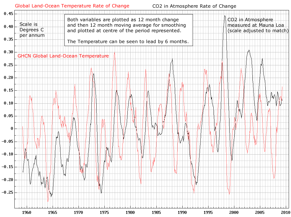

This falsifies any hypothesis that a change in T causes a change in CO2.
Wrong. On time scales from years to hundreds of millennia, the causation is clear. ∆T causes ∆CO2:
And:
[click in chart to embiggen]
(Note the NOTE in the chart.)
A fool argues with real world, empirical evidence, while honest skeptics accept what Planet Earth is saying. The planet is clearly showing that ∆CO2 is caused by ∆T.
BLAM! Way — to — go, D. Big Gun Stealey! Another Science Giant fires off a devastating artillery round. We privates down here in the infantry appreciate it!
1old,
“Per Lord Monckton”? You need to cut and paste the quote. I’m too lazy to find it, but I think Lord M was referring to the zero trend in global T for the past 18+ years.
Furthermore, what’s your point? My point is that the real world shows that CO2 does not have the global warming effect claimed.
If that is the case, then the climate alarmists’ scare is falsified.
The “dangerous AGW” alarm was all predicated on evil “carbon”. Since Planet Earth is debunking the CO2=cAGW scare, we can just forget about our ‘carbon footprint’, and all the rest of that nonsense.
They were wrong, case closed.
oldsocrates says:
My point is that when you post “∆T causes ∆CO2” you are wrong
When I post that ∆T causes ∆CO2, I am correct. See, I post corroborating links that support what I write, while you just give your opinion.
Next, when I post that global warming has stopped, that is based on the satellite measurement temperature trend; the most accurate global temperature data available. Again, when you dispute that, it is based on your opinion, nothing more.
And you are still not quoting Lord M verbatim. All you’re doing is arguing with everyone. Well, here’s a news flash: they’re right, and you’re wrong. If you don’t think so, check out the numerous links being posted. What have you got, beside your opinion?
oldsocrates:
Two “facts”? Nope. You said:
∆T for the past 17/18 years has been zero.
Wrong — as I’ve schooled you. But you don’t learn.
And the change in CO2 is just a deflection, as usual.
Since your first ‘fact’ was wrong, your premise is in big trouble. As usual.
oldie,
Either give me the temp you need for a particular year, or the trend you need for a specific time frame. I can provide either one.
…On second thought, you need to get up to speed on this subject. I suggest reading the WUWT archives for a few months. That will at least get you started. As it is right now, you’re asking 7th grade questions, and I’m not interested in holding your hand any longer.
Oldandwise- the production of CO2 from outgassing of the oceans isn’t instantaneous so the delta T that has taken place could be responsible. Certainly, temperatures turned flat after the super el nino in 1998 but, like when you strike a baseball, the ball goes for quite a ways after the impact.
old1,
Stop with your obfucating and nitpicking. Monckton was referring to the zero change in trend.
When you say:
That means ∆T = zero for 18 years and 9 months.
…are you being dense? Do you really believe there was NO change in global T during those 18 years??
If you do, we’re through here. You’re too stupid to respond to. Alzheimer’s, no doubt.
But if you’re just playing juvenile word games, then you’re being a site pest. That means you’ve got nothin’. If you had worthwhile facts, you would use them. But since you’ve got nothin’, you play your word games.
That’s about the level of the commenters here who believe in the ‘dangerous AGW’ false alarm. No facts, no evidence, and the real world is making fools of them.
So carry on.
What do I say?
I say you’re a site pest who doesn’t understand the first thing about hte subject… David.
I could post a dozen charts showing that global T is different every year. I could post charts showing the flat trend in global T. But nothing will satisfy you, because you have no interest in learning anything, you’re just running interference. Go back to hotwhopper where you belong.
Does that mean I win?
It means I’m on to you. You have no interest in learning anything; you’re just interested in arguing incessantly.
This article is about CO2, which your alarmist cult claims is the cause of global warming. Not just that, but ‘runaway global warming and climate catastrophe’.
But when that didn’t happen, it was changed to “climate change”. Because that always happens.
Now that the ultimate Authority, Planet Earth, has debunked your false alarm, you have two choices:
You can accept what reality is telling you; that there is nothing unusual happening, or…
You can obfuscate, deflect, endlessly nitpick, try to run interference, and ask interminable questions like a seven year old asking “When are we gonna get there?”
You’ve chosen the second course of actions, because some folks just can’t ever admit that their conjecture has been debunked.
Oldn: “Does that mean I win?”
LOL.
How could it? You have yet to get up out of your seat in the bleachers and down onto the playing field. D. B. (and along with others) has been engaging in excellently skillful play on the playing field. You have yet to make one genuine argument/play. No, Old, sorry, but empty comments called out at the ref or the players on the field are not “playing.”
Lol, let the poor sod think he “won,” D.B.. The rest of us can see what the deal is.
Not Altzheimer’s, perhaps, but, there is SOMETHING wrong. THAT is certain, proven by the words from Old’s own mouth.
At least, D. B. your fine play/presentation of evidence refuting AGW helped those who were genuinely interested in learning. Your efforts were not wasted, even if they were utterly wasted on Old.
1oldnwise4me@reagan.com
∆T has been near zero for the past 18 years.
Your “argument” is nothing but a distraction to the discussion of whether a decade-long change in CO2 causes a decade-level measurable change in global average temperature.
The ice core records are not sufficiently accurate in discerning individual year-to-year differences (CO2 immersion factors or CO2 equilibrium rates at that fine a time scale (10-20 years)) to determine if ever, nor if never, nor how many times ∆CO2 changed over a dozen year record to make any absolute claim. There is no indication either way.
Just as weather (individual days of temperature, humidity, rainfall, wind, or pressure) changes much more dramatically than does “climate” (now claimed to be a 30 year running average of all the above variables), the ice core records can determine hundred-year trends of CO2 and temperature reliably, but year-to-year trends (changes) with almost no reliability. It is two different cause-and-effects entirely over the short term. Jumps in temperature CANNOT immediately change CO2 since the thermal mass of the oceans and grounded CO2 take many years to warm enough ocean water to release enough CO2 to make a measurable change in global average CO2 levels.
On the other hand, the entire CO2 CAGW scare requires a near-immediate response of temperature to a change in CO2. That has been falsified the past 20 years, the past 60 years, the past 450 years, the past 1000 years, the past 3000 years.
A single “air bubble” trapped between ice layers actually crosses many years of seasonal ice layers. Diffusion limits (the number of layers of ice required to “stop” CO2 from diffusing “up” (more recent) or “down” (older) cover a short but definite period – usually accepted as 70 years.
Thus, to claim any single “year” for any single “CO2 level” is wrong. Dead wrong and misleading. Distracting. Trying to extract any year-to-year trends over any interval less than 100 years is foolish, wrong, and deliberately incites of misleading the understanding of other readers.
The temperature is no where near the projections or the 95 % certainty level. The only thing CAGW has is yelling about the warmest year ever. Which is almost laughable if this discussion weren’t so serious. No matter which way you look at it, CAGW is in huge trouble. If AGW is right, temps are falling. But doesn’t co2 control temperature? And if AGW is wrong, the temperature chart kind of looks like it does now. No relationship whatsoever. Co2 is in one direction, up, and temperature is either flat or declining. I can point to various arguments the IPCC has recently put forth to explain the pause. (excuses). Last look there were about 30.
1oldnwise4me@reagan.com
False. You are trying to distract the falsification that the ice core records show, by trying to “create” some requirement that a short change in temperature immediately changes global CO2 levels. Global CO2 levels have changed recently, and – over the same time period, global average temperatures have not changed. But that does NOT falsify the ice core records that integrate dozens of years of CO2 changes into a longer record of several tens of thousands of years when CO2 has NEVER led temperature changes.
Two different effects. Two different measurements.
Central California has had thousands of earthquakes the past 200 years, but none over magnitude 4.0
Northern CA had a massive earthquake in 1903 moving its fences and buildings 8 feet in one day.
Southern CA has not had a magnitude 7+ earthquake since statehood.
How far does an earthquake move the dirt in California?
old,
The red line shows annual temperatures. The green line is the trend:
http://realclimatescience.com/wp-content/uploads/2015/06/ScreenHunter_9549-Jun.-17-21.12.gif
Your question was a lame attempt at a “gotcha”. But you’re not smart enough to pull that off.
old1,
I’ve answered below. Now it’s your turn to do some ‘splainin’.
1oldnwise4me@reagan.com November 27, 2015 at 1:59 pm
I am going to respond to this silliness one more time. What good it will do, I do not know.
We have
dCO2/dt = k*(T – T0)
That means for small time step ∆t, we have approximately
∆CO2 = k*(T – T0)*∆t
which is to say that
1) CO2(t+∆t) = CO2(t) + k*(T – T0)*∆t
That means that, if at an additional time step ∆t, if temperature has risen ∆T, we will have
2) CO2(t+2∆t) = CO2(t+∆t) + k*(T+∆T – T0)*∆t
Thus, subtracting (2) from (1), we find
3) CO2(t+2∆t) = 2*CO2(t+∆t) – CO2(t) + k*∆T*∆t
Thus, even if ∆T = 0, we still have
4) CO2(t+2∆t) = 2*CO2(t+∆t) – CO2(t)
Suppose CO2(t) = 399 and CO2(t+∆t) = 400. Then
CO2(t+2∆t) = 401
CO2(t+3∆t) = 402
CO2(t+4∆t) = 403
CO2(t+5∆t) = 404
CO2(t+6∆t) = 405
and so on. It keeps going up linearly.
David Socrates a.k.a. 1old apparently thinks ∆T = T – T0. This is incorrect. T0 is a constant in the model, and ∆T = T(t+∆t) – T(t).
Except that Bart forgets that dCO2/dt also responds to increased pressure in the atmosphere…
The in/outflux of CO2 between oceans and atmosphere is directly proportional to the pCO2 difference between atmosphere and oceans.
Take the pCO2 at the upwelling waters near the equator: a pCO2 of ~750 μatm. Atmosphere at ~400 μatm (~ppmv). ∆pCO2 = 350 μatm. Influx (into the atmosphere): about 40 GtC/year (absolute figure not of interest here).
As the local temperature didn’t increase in the past 18.5 years, the 40 GtC/year is constant. T-T0 = 16°C
The same at the other end of the oceans, near the poles:
pCO2 of the oceans: ~150 μatm, atmosphere ~400 μatm, ∆pCO2 = 250 μatm, outflux ~40 GtC. T-T0 = -17°C
Overall balance: dCO2/dt = 0, T – T0 = 0, influx = outflux = 40 GtC/year.
Suppose that T goes up everywhere with ∆T = 1°C
At the equator, according to Henry’s law for ∆T = 1°C:
Oceans: 750 + 16 = 766 μatm. ∆pCO2 = 366 μatm. Influx 40 * 366/350 = 41.8 GtC/year. T+∆T – T0 = 17°C
At the poles, according to Henry’s law for ∆T = 1°C:
Oceans: 150 + 16 = 166 μatm. ∆pCO2 = 234 μatm. Outflux 40 * 234/250= 37.4 GtC/year. T+∆T – T0 = -16°C
Initial increase in the atmosphere: 1.8 + 2.6 = 4.4 GtC/year or ~2.1 ppmv/year.
As the CO2 levels in the atmosphere increase, the pCO2 pressure difference with the oceans increases at the upwelling side and the decreases at the uptake side. That reduces the influx and increases the outflux. At the moment that the pressure increase in the atmosphere reaches 16 ppmv, the original pressure differences are restored and thus the original equal input and output fluxes and no further CO2 increase is happening. In graph form (the real half life time may be shorter):
http://www.ferdinand-engelbeen.be/klimaat/klim_img/upwelling_temp.jpg
That is the transient response of the ocean – atmosphere system to ocean temperature changes.
“Except that Bart forgets that dCO2/dt also responds to increased pressure in the atmosphere…”
It’s in my model, Ferdinand. It’s all there. You are wrong. An accumulation of CO2 in the surface waters naturally results in an accumulation in the atmosphere. Far from being a limiting factor, Henry’s Law is what enforces the increase in the atmosphere.
No doubt, over long-enough time-scales, changes in temperature produce changes in atmospheric CO2 concentrations through oceanic solution. But that doesn’t preclude other mechanisms (organic decay, AG emissions) from contributing independently to CO2 changes. Strong correlation is insufficient, however, to distinguish between various causes. The critical question is the dynamic response characteristics of CO2 to each factor. That is best established through proper cross-spectrum analysis, which is very rarely done competently in “climate science.”
ioldwise makes a point. He is talking about a different scale than micro wiggle matching. He is asking why atmospheric dCO2 didn’t slow to match the crawl if it was all dT and none human. Pretty much like asking why atmospheric levels are so much higher today than observed during prior periods of higher temperatures. Maybe that’s the derivative thing. It increases sensitivity to micro accelerations at a scale where they matter.
Old is mixed up, O Generous Gymnosperm:
He is soundly thumped by Bartemis above:
Bartemis, here: http://wattsupwiththat.com/2015/11/25/about-spurious-correlations-and-causation-of-the-co2-increase-2/#comment-2080833
(and I pointed out the following, basic, but, that’s the level of Olds’ comments):
“1old: additionally
1) your time scale is too short; and
2) you also need to factor in that CO2 level lags temperature by a quarter cycle (did you watch the above-linked video (you can find it with a quick search on youtube directly, too) of Murry Salby’s Hamburg, 2013 video? — if so, I think you need to watch it again — his teaching is quite clear to a layperson such as myself).
It’s too soon to say Bartemis and Salby are incorrect, much less, “falisified.”
Me, here: http://wattsupwiththat.com/2015/11/25/about-spurious-correlations-and-causation-of-the-co2-increase-2/#comment-2080904 (affirmed by afonzarelli as to the emphasized clause, here: http://wattsupwiththat.com/2015/11/25/about-spurious-correlations-and-causation-of-the-co2-increase-2/#comment-2081079).
As I pointed out above, old1 conflates his terms. He’s deliberately trying to frame the question so if I say it’s the trend, he will pull a ‘gotcha!’ and talk about the change in global T year to year. But if I answer with the change in intra-annual temperatures, he will move the goal posts and pull another ‘gotcha!’, claiming that the trend shows “zero” ∆T.
But as I pointed out above, he’s just not smart enough to pull that off.
Here’ a chart showing both the change in annual temperatures, and the trend:
http://realclimatescience.com/wp-content/uploads/2015/06/ScreenHunter_9549-Jun.-17-21.12.gif
And now it’s my turn to ask a question: does the old1 think that the change is instantaneous? That there’s no lag time between CO2 and T (or T and CO2)?
So instead of his interminable ‘gotcha’ questions, how about if old1 explains exactly what he thinks the situation is? This should be good. Will he answer?
OK old1: On your mark… Ready… GO!
oldie,
I’ve answered several questions now. And I note that the alarmist contingent has one thing in common: they always want to ask the questions (which are then followed up by more questions, etc.) But they never want to answer any questions. You completely avoided my question above.
So first, old1, you answer my question. Explain what you think is happening. Give us your CO2/temperature narrative. Explain how “carbon” is gonna getcha. (And if you think CO2 isn’t a problem, then explain why you’re thread-bombing when it doesn’t matter.)
See, I don’t know for certain where you’re coming from, or what you believe.
You’ve been hiding out. Time to explain yourself.
He DID explain himself very clearly! He said:
The above two facts are all that he wants addressed. Forget ice cores; forget lag times; forget warming due to CO2. Those are NOT what he is talking about.
1oldy1,
Where are you coming from? What is your ‘carbon’ narrative? Is there anything to the CO2 scare? If so, explain what you think it is. Or are you just thread-bombing?
This is the 4th time I’ve asked you questions. I’ve answered yours, but you continue to ask more questions. Enough of that, now it’s your turn to post some answers. I’ve never gotten any answers from old1 in response to these comments:
• “…how about if old1 explains exactly what he thinks the situation is?”
• “…it’s my turn to ask a question: does the old1 think that the change is instantaneous? That there’s no lag time between CO2 and T (or T and CO2)?”
• “…I’ve answered below. Now it’s your turn to do some ‘splainin’.”
• “…old1, answer my question…”
I’ve answered several of old1’s questions, using charts, logic, and real world observations. But the old1 still hides out from answering any questions that I ask. He doesn’t understand the concept of quid-pro-quo. Now it’s his turn to answer some questions of mine.
Will old1 explain himself? Or will he skedaddle rather than answering questions?
(Werner, he is unclear. Is it temperature in a specific year, or the temperature trend? I’ve asked that, but he doesn’t answer as usual. Maybe you would like to answer, if you know what he’s asking. I don’t.)
Hi Werner B,
Here is a chart showing that T leads CO2 by six months:
That is a real world observation. The causation is crystal clear: ∆T causes ∆CO2. But oldy says T never changes!
We see the same cause and effect relationship in this WoodForTrees chart. In fact, we see the same causation on many differnt time scales:
http://theinconvenientskeptic.com/wp-content/uploads/2010/09/Vostok-CO2.png
old1 is claiming that there is zero change in T, while CO2 is rising. That makes no sense to me. Furthermore, he deflects from the question of lag time, as if it doesn’t exist.
We see in the chart above that T is never zero. Therefore, old1 is not making any sense when he claims that ∆T is zero.
I should add (before the discussion gets too far afield) that the basic alarmist premise stated that a rise in carbon dioxide would cause runaway global warming. That is the claim that started it all.
So naturally, since the alarmist crowd’s belief in CO2=cAGW has been so decisively debunked by the real world, they now want to deflect to other, extraneous arguments that try to hide the fact that they were proven to be flat wrong.
Anyway, perhaps you can understand what the old codger is saying; it’s unclear to me. If so, you can try to answer him. He is not being coherent. As Janice says, “Old is mixed up”.
Before I answer any more of his questions, oldy owes me a few answers first. I’ve already answered him several times. Now it’s his turn to answer a few questions of mine.
Maybe that’s why he seems to have skedaddled. Alarmists always want to be the ones asking all the questions, but they never answer any. It’s time for 1old1 to man up, and start explaining himself.
Yes, I know exactly where he is coming from. (But should I be wrong, he can always correct me.)
Here: http://wattsupwiththat.com/2015/11/25/about-spurious-correlations-and-causation-of-the-co2-increase-2/comment-page-1/#comment-2081114
you say: “Wrong. On time scales from years to hundreds of millennia, the causation is clear. ∆T causes ∆CO2:”
So his question is: Does this apply over the last 18 years and 9 months where RSS shows no change and CO2 is up by 30 ppm? We are NOT talking about seasonal variations nor warmer and colder years having some influence since 1997. Rather, why did the CO2 not stay more or less at its 1997 level?
Ferdinand Engelbeen has this to say:
“The point where Bart (and Dr. Salby) got wrong is where he saw a perfect match of the variability’s and assumed that the slope was from temperature too.
Thus while temperature and other natural causes are fully responsible for the variability, temperature is not responsible for most of the increase, human emissions are… “
See: http://wattsupwiththat.com/2015/11/25/about-spurious-correlations-and-causation-of-the-co2-increase-2/comment-page-1/#comment-2081102
Do you not agree with Ferdinand?
Werner Brozek (4:46am, today): Your “two facts” are not “fact” at all. The assertion you cite as Olds’ “facts” is unsupported, nonsensical (puts the effect before the cause — CO2 began to slow in increase around THE SAME TIME as temperature flatlining around 1998), sophomoric, and insincere (or crazy — take your pick), JUNK.
Why a normally fine thinker as you would defend such an empty-minded, disingenuous, troll is intriguing… .
Do you KNOW this “Old”? IS HE YOU POSING AS A SOCK PUPPET?? lol, if so, way to go, Brozek — you did a good job, oh, brother, WHAT a sock-puppet!
Huh? Here is RSS for 18 years and 9 months:
http://www.woodfortrees.org/plot/rss/from:1997.05/plot/rss/from:1997.05/trend
Both dbstealey and Lord Monckton agree with this.
Here is CO2 since 1958:
http://www.woodfortrees.org/plot/esrl-co2/from:1958
It shows an increase from about 360 to about 395 since 1997 with no decrease in rate since 1997.
Which fact is wrong?
(No, I did not pose as anyone else.)
Werner – the relationship is dCO2/dt = k*(T – T0), where T0 is an equilibrium temperature, and k is a coupling factor (remarkably, essentially constant since at least 1958).
The rate of change has leveled off since the “pause” commenced. What you are doing is akin to tracking a spent rocket in space and claiming that, since its velocity hasn’t changed while you observed it, the rocket engine isn’t responsible for its speed.
I agree with that. However it is still going up at a steady rate. In my opinion, only human emissions are responsible for that steady increase. Let us suppose this pause on RSS lasts for another hundred years and CO2 goes up steadily at the present rate to 550 ppm, what would you attribute it to?
If your answer is different from Ferdinand’s, I will apply occam’s razor and agree with Ferdinand.
“However it is still going up at a steady rate.”
Yes, and that rate is consistent with the dCO2/dt = k*(T – T0) relationship.
“Let us suppose this pause on RSS lasts for another hundred years and CO2 goes up steadily at the present rate to 550 ppm, what would you attribute it to?”
If the relationship dCO2/dt = k*(T – T0) continued, I would attribute it to temperature. If some other relationship came to the fore, I would consider that.
Obviously, dCO2/dt = k*(T – T0) with T exceeding T0 cannot last forever. This is a local model. It holds, with remarkable fidelity for constant k and T0, for the past 57 years.
Local models are used in engineering all the time. The transistors in your electronic gadgets are biased to operate in a linear range, and the gain is computed on that basis. That does not mean, however, that you can extrapolate the gain such that an input can be amplified beyond the supply voltage.
The local model is enough to tell us what has been dominating atmospheric CO2 evolution for at least the past 57 years. It is enough to tell us that natural processes are currently in the driver’s seat. To determine a global (in a mathematical sense) model, we will have to continue our observations over a long enough timeline that other dynamics become observable.
Note: when I say “observable”, I mean it in a particular technical sense.
Janice – Oldie is not Werner. He is the old “David Socrates” sock-puppet. Only he can continue droning on and on with the same baseless objection without understanding that it is been refuted over and over again. Only he can look at a plot plainly showing dCO2/dt = k*(T – T0) and claim that a lack of change in T results in a lack of change in CO2.
Bart:
The local model is enough to tell us what has been dominating atmospheric CO2 evolution for at least the past 57 years.
No, it doesn’t tell such a story, as it is not a unique solution. My solution shows the same variability an exactly the same slope without arbitrary offset and factor for the slope with human emissions plus natural variability. Without violating Henry’s law for the solubility of CO2 in seawater.
Your solution ignores the negative feedback from the increased CO2 pressure in the atmosphere: if that passes the 16ppmv/°C change, CO2 is pushed into the oceans, not reverse…
“My solution shows the same variability an exactly…”
Your solution is not physically valid. If your natural input is attenuated by a 40 year time constant, then your anthropogenic input also has to be attenuated by a 40 year time constant.
I know you didn’t do that because attenuating the input that way results in a loss of polynomial degree – the anthropogenic input does not continuously accumulate, but settles into a proportionality with the input rate of change.
Bart:
If your natural input is attenuated by a 40 year time constant, then your anthropogenic input also has to be attenuated by a 40 year time constant.
I used a 51.3 years time constant (~40 years half life) for any pressure above steady state of the oceans. That is the same for human as well as for natural causes of the extra pressure.
That is completely independent of the 12 month time constant that temperature has on (tropical) vegetation, as that releases CO2 into or takes in CO2 from the atmosphere, whatever the origin of that CO2.
Temperature is responsible for almost all the variability and a small part of the slope.
Pressure is responsible for almost all the slope…
Ferdinand, i dispute the henry’s law value of 16ppmv/1C as represented in ice cores. In much the same manner that we can say that south pole temps aren’t reflective of global temps, neither are the co2 concentrations reflective of reality. If we just look at the long closing time of the bubbles alone, all peaks and troughs are smoothed, lessened in amplitude, so that they under represent the value of henry’s law…
I don’t know what you did, Ferdinand, because you haven’t written it down. But, I know you didn’t apply a time constant parameterized low pass filter to the anthropogenic data like you did to the temperature parameterized data because of the aforementioned polynomial degree discrepancy.
I am simply an observer in this discussion. Much has been debated as to sinks and sources of the atmospheric C02 cycle. A recurring thought in my mind over several years and discussions/debates is as noted. What is the effect of falling rain with regards to CO2 levels?
I would assume that rain begins at a temp of about 0C and falls through the atmosphere where it should absorb CO2. Much of that probably falls in the oceans. I would guess that in itself would classify rain as a sink. Has there ever been any research as to the amount of CO2 that would be affected by this process? Just saying.
eyesonu,
I have calculated that some time ago: not important at all. Fresh water absorbs a few mg per liter at 0.0004 bar pressure in the atmosphere. If rain is formed, that needs about 400 m3 air to form 1 l of rain, the absorbed amount of CO2 out of 400 m3 air is undetectably low. When that falls on 1 m2 ground and all water evaporates, that increases the adjacent 1 m3 air with less than 1 ppmv if there is no wind,,,
Still huge quantities of CO2 are lifting with water vapor from the equatorial seas to where the rain falls, but back on the oceans that is just a cycle. On land it can dissolve carbonate rocks, but even that needs millions of years the form the beautiful caves…
Thank you for your reply.
Through ‘google’ search I have been able to find that rain can have a PH varying from ~4.5 to 6.5 in the USA alone. That would seem to imply that considerable CO2 was absorbed. That which falls on land and soaks into the ground would seemingly carry some amount of CO2 into the soils.
Again I thank you for your reply. The discussion on this thread has been captivating from my perspective. You have done an excellent job with regards to responding to other comments. I wish I had the knowledge to pick the scientifically correct process (if only one exists) in the discussion. But it has been a learning experience and is an excellent example of scientific discussion where differing views are debated. As I noted in an earlier comment, I hope some in the academic professions will use this thread as an example of how science should be debated and progress. You opened the door on that one.
eyesonu,
Thanks for your kind words…
You need not much CO2 to lower the pH to ~4, a few mg is sufficient as there is no buffer in fresh water. Other acids may help too: SOx, NOx,… if the air is polluted.
For the solubility of different gases in fresh water see:
http://www.engineeringtoolbox.com/gases-solubility-water-d_1148.html
That is for 1 bar pressure or 100% CO2 in the atmosphere.
At 0.0004 bar partial pressure in the atmosphere it is a few mg/l.
http://wattsupwiththat.com/2015/10/24/water-vapour-the-big-wet-elephant-in-the-room/#comment-2057601
Hi Ferdinand,
I am glad that you were respectful to Ernst Beck – many others were not.
To be clear, I regard you as one of THE experts on this topic, and enjoy your thoughtful comments.
Having said that, I am still an agnostic on your key conclusion – the “mass balance argument” (MBA) that concludes that fossil fuel combustion is the most significant driver of the observed increase in atmospheric CO2. I just want to wait and see what the new CO2 satellite data tells us.
We can afford to be patient on the MBA issue, since it is increasingly obvious that the sensitivity of global temperature to increasing atmospheric CO2 is too small to be significant.
Other issues are much more important and urgent:
IF we are correct about imminent naturally-driven global cooling, which some of us think should be apparent by 2020 or sooner, and which could be mild or severe, then we cannot wait much longer to address the potentially serious consequences of cooling on society.
As I have stated before, I hope to be wrong about cooling.
Best, Allan
Hi Allan,
The mass balance is not the only argument, human emissions as cause fit all observations…
But we agree on the part of the impact of the extra CO2…
http://wattsupwiththat.com/2015/01/30/what-are-your-fears-about-global-warming-and-climate-change/#comment-1847733
Hypothesis:
1. The next act of this farce will be characterized by global cooling starting by about 2020 or sooner, cooling that may be mild or severe. Global cooling will demonstrate that climate sensitivity to increasing atmospheric CO2 is so small as to be insignificant. The scientific credibility of the warmist gang will be shattered and some may face lawsuits and/or go to jail.
2. The scientific community will gradually accept the fact that CO2 lags temperature at all measured time scales, and that temperature (among other factors) drives atmospheric CO2 much more than CO2 drives temperature.
3. The foolish green energy schemes to “stop global warming” will be shelved and dismantled, but not before they contribute to a significant increase in Excess Winter Mortality, especially in Europe and to a lesser extent in North America, where energy costs are much lower (thanks to shale fracking).
4. The warmist thugs will still be bleating about a warmer world, wilder weather, etc., all caused by the sins of mankind, but nobody will listen.
Regards to all, Allan
with reference to Engelbeen and 10:48 am. Sorry I don’t seem to be able to reply in thread. First a general comment, it disturbs me that so many people casually dismiss the work of earlier scientists as wrong or inaccurate often on the most flimsy of evidence. In reading up on the history of science what stands out is the inordinate lengths that scientists in the past went to to achieve more and more accuracy in their measurements. There are examples of where theories were destroyed by measurement discrepancies in the 3,4 or 5th decimal place.
WRT to CO2 measurement, firstly an accuracy of +-10 ppm which you quote is adequate to determine the trends we are looking at. Secondly these people were not fools, and they did understand the impact of measuring CO2 in the middle of a town or forest. There are stories of scientists making arduous journeys to remote coastal places just to make their CO2 measurements more representative. This issue of poor measurement siting also does not explain the similarity of measurement done by different scientists at similar times. If it was all siting dependent then different scientists measuring at the same time but using different sites should get wildly different results. Scientists in the future could just as well argue that measuring CO2 on a volcano (Mauna Loa) which is spewing out CO2, as Mauna Loa does, is a really questionable approach and justifies ignoring all the data so collected.
WRT pH measurement. Your comment that glass electrodes were the earlier (relatively inaccurate) way of measuring pH since replaced by the colorimetric approach does not agree with my research. The earliest methods of measuring acidity were colorimetric ones using substance like Litmus (discovered in 1300 and used since). The glass electrode was only invented in 1909 and was far more accurate than the earlier methods (certainly not in existance for the last 165 years). True, spectroscopic methods of measuring colour change instead of relying on subjective comparisons against a printed colour chart have improved consistency but, as someone who has designed and built spectroscopic equipment for making such measurements (my job is doing research for a spectroscopy company), I can tell you the human eye is incredibly good at picking up colour differences and it is really hard to get a spectrometer to do any better. Non the less, today the most common method of measuring pH is via the glass electrode.
Michael,
I am sure that the scientists of the pre-Mauna Loa period were very good in what they did. But you need to take into account that the methods used were not even good enough to measure the seasonal changes. Even Keeling Sr. was surprised to see a clear seasonal signal after a year of data at Mauna Loa. The longer term changes also were minimal at that time, although slowly emerging out of the background noise.
Callendar was the first to use stringent a-priory criteria to sift between the noisy data, like “not from agricultural research”, which should eliminate the 1943 “peak” in Beck’s compilation as that is mainly based on two long series used for agricultural purposes… One can have objections against Callendar’s criteria (like “less than 10% deviation from the average”), but at least he had criteria and his estimates were confirmed decennia later by high-resolution ice cores…
This issue of poor measurement siting also does not explain the similarity of measurement done by different scientists at similar times.
You really should look at the data which were compiled by the late Ernst Beck: near 400 ppm at Giessen, Germany, in the same year 250 ppmv somewhere near Chicago (if I remember well). Here the minima and averages of different series taken in the same year and from different years compiled by Ernst Beck:
http://www.ferdinand-engelbeen.be/klimaat/klim_img/beck_1930_1950.jpg
The maxima were near all off-scale…
There were few ocean (ships) and coastal air CO2 measurements in the whole compilation and these are all around the ice core data…
About pH measurements: glass electrode measurements in seawater are not that easy and as you need an accuracy of better than 0.01 pH unit to see a change of 0.1 unit over a time span of 165 years, quite impossible. The only alternative is calculating the pH form other measurements (total alkalinity,…)
Spectrophotometric is better than electrochemistry. 0.0007 pH units in one method
Let’s sneak in there when noone is lookin’ and substitute true random noise for all this seemingly random data and see if we come out with the same results. If we do, let’s arrest them all and demand a full refund. Those that refuse will be turned over to the Saudis for beheading.
Source: random.org
Werner writes:
“Ferdinand Engelbeen has this to say:
“The point where Bart (and Dr. Salby) got wrong is where he saw a perfect match of the variability’s and assumed that the slope was from temperature too.
Thus while temperature and other natural causes are fully responsible for the variability, temperature is not responsible for most of the increase, human emissions are… “
An excellent summary. One we all might have divined from Ferdinand’s work but for distractions. Second derivatives explain the variability, but not the trend.
The question becomes, why doesn’t the variability explain the trend? It really ought to. We humans are new players. Not omnipotent players, but new nonetheless.
Going forward many questions remain to be answered. What exactly does “most of the increase” mean? Ferdinand would have it be 95% based on Henry’s law. Yet our understanding of the oceans is so poor the IPCC thinks 3Gt of ocean biomass produces a 50Gt flux. Ocean biology is a wild card exempt from Henry’s law. Our understanding of soil respiration is so bad we were all stunned to see substantial net CO2 coming from the southern margin of the boreal forest.
IMO there is ample margin to suppose the human liability is far less than 95%. What if it were 50%?
A world of difference.
gymnosperm,
Just a matter of different processes: all the variability is from a temperature sensitive process, mainly by (tropical) vegetation. That reacts very fast (half life less than 1 year) but limited: some 4-5 ppmv/°C. Oceans are slower (at least 4 years, but maybe longer) but have a larger response: ~16 ppmv/°C.
Near all the slope is caused by human emission, as the decay rate is by pressure sensitive processes, a small part in vegetation, a larger part in the oceans, in direct proportion to the difference in pressure between the atmosphere and the ocean surface / plant alveoli’s water interface. The overall sink rate currently is ~2.1 ppmv / 110 ppmv extra pressure in the atmosphere or an e-fold decay rate of over 50 years or a half life time of less than 40 years. Too slow to remove all human emissions in the year that they were released. That is the case for every year of the past 57 years…
Temperature has a small contribution to the slope, due to a small non-linear increase of CO2 in the dynamic equilibrium with temperature: less than 10 ppmv in the past 57 years, ~10 ppmv over the past 165 years from temperature alone.
That another unknown process did substantially add to the total increase is theoretically possible, but in that case, the alternative source must fulfill following conditions:
– increase a fourfold in quantity over the past 57 years in lockstep with human emissions, as the sinks don’t discriminate between the origin of the emissions.
– have the same low δ13C level as human emissions.
– don’t change the total carbon circulation, as there is no sign of a shorter residence time.
Which is hardly possible…
To increase fourfold in 57 years requires a 7% annual increase (unless I need more coffee). Since soil respiration is thought to be 6 times human production, I believe you can divide that 7% by 6 to get something more than 1% annual increase to satisfy the condition.
Soil respiration has a 13C signature in the same range as human combustion.
Soil respiration has been around since substantial soils developed in the Devonian as an integral part of the Carbon cycle, satisfying the third condition.
A 1% annual increase in soil respiration during the natural warming + whatever tiny human warming over the last 57 years seems possible, and some increase certainly took place…
gymnosperm,
Soil respiration is part of the total biological carbon cycle. That cycle is negative: more sink than source…
Most of soil respiration and plant decay is aerobic, what isn’t is methane, but that is oxidized in the upper troposphere by OH radicals with a half life time of ~10 years. Thus even if there was an increase in methane release, that is far from a 4-fold, as the CH4 levels are hardly increasing in the atmosphere.
Ferdinand, the biosphere may be a net sink, but individual components need not be. Carbon cycles typically portray soil respiration as ~60Gt out and ~.2Gt in. Essentially a one way input like human combustion.
It is true that most soil respiration is aerobic. Respiration increases from dry to about 60% saturation and at higher water content respiration decreases and becomes more anaerobic. Many soil microbes have multiple metabolic pathways at their disposal and simply switch from O2 as an electron acceptor to something else and continue to produce CO2 rather than methane.
Soil water saturation is not uncommon. Pretty much whenever it rains. But if only 25% of soil respiration were anaerobic, it would hide an amount of respiration 1.5 times human production from the oxygen balance.
gymnosperm:
Ferdinand keeps making the untrue assertion of “different processes”. The assertion is wrong as I explain to him repeatedly in this thread and most recently here.
The observed rise in atmospheric CO2 concentration may be entirely natural, or entirely anthropogenic, or some combination of the two. What is certain is that Ferdinand’s narrative is wrong as I have yet again explained to him in the comment I have linked.
Richard
Clearly temperature did not cause human combustion. That is the only sense in which the processes are different.
gymnosperm,
Richard doesn’t understand the importance of the different processes: temperature is good to explain a lot of the year-by-year variability, but doesn’t explain the increase, while human emissions explain all the increase and nearly nothing of the variability. The difference between human emissions and increase in the atmosphere is by a pressure regulated process, largely independent of temperature and vv.
That is explained in depth under the comment of Richard…
Ferdinand Engelbeen:
You say to gymnosperm,
Ferdinand, I do “understand the importance of the different processes” that you misrepresent.
To save people needing to look up the reality, I copy here my most recent attempt to get you to see sense in this thread.
I wrote to you
Richard
gymnosperm November 28, 2015 at 6:30 pm
“Second derivatives explain the variability, but not the trend.”
Actually, I do not know where you are getting “second derivatives”. The relationship is
dCO2/dt = k*(T – T0)
There is only a first derivative there. It does not affect the trend in dCO2/dt, which is clearly caused by the trend in T.
Human inputs also have a trend. But, that trend is already explained by the temperature relationship. Ergo, human inputs are not affecting that trend significantly, and hence, are not having a significant impact overall.
Hello Ferdinand
I tried to access Mauna Loa (MLO) CO2 data today and found these NOAA databases that only go back to 1974 or 1969.
ftp://aftp.cmdl.noaa.gov/products/trends/co2/co2_weekly_mlo.txt Starts 1974 05
ftp://aftp.cmdl.noaa.gov/data/trace_gases/co2/in-situ/surface/mlo/co2_mlo_surface-insitu_1_ccgg_MonthlyData.txt Starts 1974 01
ftp://aftp.cmdl.noaa.gov/data/trace_gases/co2/flask/surface/co2_mlo_surface-flask_1_ccgg_month.txt Starts 1969 08
My previous work years ago accessed MLO data back to 1958, presumably when Keeling stated colleting data there.
ftp://ftp.cmdl.noaa.gov/ccg/co2/trends/co2_mm_mlo.txt
Any idea why data pre-1974/1969 is apparently no longer on the NOAA site?
Regards, Allan
Allan,
Indeed, a lot of ftp sites are gone. Maybe a temporarily failure of the site, or they are moving the old date to a different map… The modern data still are there via the carbon tracker, but that is from 1969 on…
We need to keep an eye on that!
Hi Ferdinand,
I just sent this:
webmaster.gmd@noaa.gov
I cannot find the CO2 data at MLO back to 1958. Where is it? Why was it deleted? Thank you.
The complete Keeling curve data is at Scripps which has run its measurement program since 1958. Right now Ralph Keeling runs the program
http://scrippsco2.ucsd.edu/data/atmospheric_co2
The NOAA series is independent of the Scripps series and started ~1974. Peter Tans runs that
http://www.esrl.noaa.gov/gmd/obop/mlo/programs/esrl/co2/co2.html
FWIW it is confusing. Worse, there have been a number of other meteorological stations on the mountain which have operated on and off and people have looked at these, and well, drawn unfounded conclusions
http://rabett.blogspot.com/2011/09/odd-introduction-to-new-paper.html
about temperature measurements at the CO2 observatory. Heavy breathing ensued.
Hello again,
I received this email from NOAA. This data goes back to 1958/9. No explanation was provided why the other data was truncated at 1969 or 1974:
A web page with the MLO CO2 data is at
http://www.esrl.noaa.gov/gmd/ccgg/trends/
A data file with the monthly CO2 data from MLO is at
ftp://aftp.cmdl.noaa.gov/products/trends/co2/co2_mm_mlo.txt
A data file with annual CO2 data from MLO is at
ftp://aftp.cmdl.noaa.gov/products/trends/co2/co2_annmean_mlo.txt
Regards, Allan
Wow, I’d need to spend a day to read all the comments properly. Seems to me the trouble is everything is linked.
Henry’s law is fine for a simple system, but the oceans aren’t simple are they? There’s life everywhere, biotic and abiotic. The rate of CO2 release from warming oceans surely has to consider the temperature difference. I accept we probably know one side of that equation – the surface temp – but we don’t know the other side – what temp was the water at before it reached the surface to outgas CO2 – well we could measure it, but even if we did, it’s only valid for a point in space, we don’t integrate it for the whole of the oceans.
Dixon,
They try to integrate it for the whole ocean surface, be it that the density of the data could be much better…
See Feely e.a.:
http://www.pmel.noaa.gov/pubs/outstand/feel2331/exchange.shtml
The CO2 level and temperature below the surface is not that important: after upwelling, the temperature and the CO2 level in the ocean waters is what makes the partial pressure (pCO2) of CO2 and the difference in pCO2 with the above atmosphere is what drives the CO2 flux in or out (at the poles)…
Is the computational mandate that temperature change occurs as a transient in response to the time-integral of net forcing (not directly with the instantaneous value of the net forcing itself) being ignored?
The fire under a kettle of water on a stove is a forcing. To heat the water, the fire must exist for a period of time. Likewise, if CO2 is a forcing, to have an effect on the temperature of the planet it must exist for a period of time. The temperature changes with time as a transient in response to a net forcing. If the forcing varies, (or not) the effect is determined by the time-integral of the net forcing (or the time-integral of a function thereof).
The observation that the temperature of the planet does not change as a transient in response to the time-integral of the CO2 level is compelling evidence that CO2 has no effect on average global temperature. The identity of the factors which are responsible for average global temperature change (97% match since before 1900) is at http://agwunveiled.blogspot.com
In assigning most if not all Keeling curve CO2 increase to non-human causes, Salby is indeed not taking into account an important factor — the so-called Revelle buffer of the partition of dissolved CO2 into aqueous and carbonate species in ocean water, which is maintained by the minerals dissolved in ocean water through buffer chemistry. Hence the exchange of CO2 between atmosphere and ocean does not obey a linear Henry’s law relationship with a reaction exponent of 1 but instead follows a non-linear 10th power law from a chain of chemical reactions having net reaction exponent of 10 (10 is best estimate of this Revelle Factor).
This power law has the effect of allowing individual atoms to freely exchange between air and ocean to account for the isotope distributions while at the same time retarding the absorption of a bulk CO2 pulse added to the atmosphere.
In Revelle and Suess (1957) “The Question of Increase of Atmospheric CO2”, even taking into account the eponymous Revelle buffer mentioned above, however, they still conjectured that most of the increase in atmospheric CO2 would not be anthropogenic but had to come from yet undetermined natural processes.
But Revelle and Suess assumed a one-compartment ocean model and did not consider a non-zero time constant for the mixing of the top 100 m of ocean with the deep ocean. I recently ran a 2 compartment-ocean carbon model taking the Revelle buffer into account, along with the exchange rate time constants between atmosphere and ocean, between surface ocean and deep ocean along with the absorption rate of CO2 by the terrestrial biosphere, which can be “tuned” to match 1) the Keeling curves for both atmospheric CO2 and C13 ratio, 2) radiocarbon age differences measured between surface and deep ocean, Revelle and Suess’ radiocarbon ages of sea shells, 3) the more recent assay of total atmospheric O2 that fixes the partition of net CO2 update from the atmosphere between inorganic (ocean carbonate system) and organic (plant uptake), and 4) the Bomb Test atmospheric C14 extinction.
Hence almost all of the increase in atmospheric CO2 can be assigned to human activity. Its a remarkable fit of 3 time constants to multiple observations of CO2 and CO2 isotope concentrations over time.
But . . .
This model that does not account for the large year-to-year variation in net CO2 emission into the atmosphere. When I tuned the terrestrial CO2 absorption to account for that variation (I added a temperature-dependent emission from the soils balanced by an increased sensitivity of plants to absorb more CO2 with increase in concentration), the human contribution to the 20th century increase in CO2 fell by half, with the remaining half the result of thermally induced emission from soils (that was my assumption from isotope trends), while still matching all of the other factors.
Furthermore, this model accounts for the observed partition of net CO2 absorption between inorganic ocean components and organic components established by the trend in total atmospheric oxygen while maintaining agreement with the isotope time series.
The fly-in-the-ointment is that not only would an increase from 280 ppm to 400 ppm seem improbable if not implausible from a natural process were CO2 totally flat-lined prior to the 20th century as indicated by the incontrovertible ice core data, but a natural process that would have increased CO2 from 280 to 340 on the time scale of 100 years is equally improbable.
On the other hand, I think there is enough evidence to doubt the temperature hockey stick but that there is an incontrovertible CO2 hockey stick, I don’t know what to think. The conjecture that the temperature fluctuation in CO2 net emissions from year-to-year having a very short time constant to not spill into the longer term trends doesn’t make sense — the famous carbon cycle graphics put multiples of the atmospheric reservoir into the living plant and the dead vegetation and soils reservoirs, and I am using those reservoir sizes in my carbon cycle model.
Is CO2 really fixed in the ice layers? Will some Galileo mutter under his breath, “But it does move!”
Paul Milenkovic:
You ask
Your “Galileo” is the late Zbigniew Jaworowski and he gave a succinct account of how “it does move” here and in this more detailed paper.
I confidently predict that Ferdinand will respond to this by saying you should ignore Jaworowski for ad hominem reasons because he cannot provide valid evidence or argument to refute what Jaworowski reported.
Richard
As you see in the above comments, Ferdinand is persistent in his arguments to say the least, and his arguments contra-Jaworowski, ad-hominen or not, are something I am going to have to try and digest. Englebeen’s arguments regarding gas exchange and the Bomb Test curve turned out to be correct in the end, but I doubt that he understood why he was correct.
I was prepared to make a public disclosure of my carbon cycle model supporting only half of the increase in atmospheric CO2 being anthropogenic along with much shorter atmospheric CO2 persistence than the Berne Model let alone the Englebeen claims.
But the “hill” on which a strong natural component to the Keeling Curve must make its stand is mobility of CO2 in the ice core. I think most people around here agree that the temperature Hockey Stick is implausible, but Ferdinand is clinging to a very definite CO2 Hockey Stick.
I don’t like Hockey Sticks of any kind, but what I like or don’t like doesn’t matter if the physics goes against my intuition. I am going to have to look long and hard at Jaworowski along with the Englebeen critique.
The way I understand Englebeen’s argument regarding Jaworowski is that the 80-year age shift between the ice core and the Keeling data has to do with 80 years of accumulated snow pack being “open” to the atmosphere before ice forms to isolate the gas bubbles, now and for eternity.
To the extent that there is an ad-hominem against Jaworowski, it is the assertion that a 1996 paper (that I will need to look at) settles the 80-year age gap with this reasoning, and that post 1996 Dr. Jaworowski has been enfeebled by age as to be no longer effectively responding to critique of his work.
A non-ad-hominem critique of Jaworowski’s claims about bringing up a core having the effect of equalizing it with the atmosphere is that there are ice cores from the Ice Ages showing CO2 at the 180 ppm level, and if contamination with the modern atmosphere in raising the cores is an effect, the true CO2 levels would be much lower than 180 ppm. Anything much below 180 is regarded as killing all plant life.
On the other hand, I really don’t think Salby’s claims on Fourier analysis of temperature and ice core time series that the ice core data had to have experienced smoothing cannot be so readily dismissed. But to support those claims, we need to look carefully at the physics, whether from Jaworowski or some other source.
Paul Milenkovic:
You say
Ferdinand has not yet responded in this thread so my prediction remains unfulfilled. However, the example you cite is a clear ad hominem: Zeb’s point was right or wrong, and his age and infirmity are not relevant to that.
You also say
I don’t think Zeb ever claimed that CO2 in a core had “the effect of equalizing it with the atmosphere”. If he did then he never mentioned it to me throughout the decades of our collaborations.
Zeb thought gases in the ice were preferentially dissolved in the surface layers of ice crystals (the surface layers are liquid at all temperatures down to -40°C) with the effect that when pressure was released by coring the gases were differently released so the air sampled from an ice core has different gaseous composition than the air trapped in the ice.
Also, ice cores “capture” CO2 because falling snow solidifies to form the solid ice. The solidification takes decades. During those decades the ice exists as ‘fern’ with open porosity.
The fern takes several years to solidify to form solid ice which ‘traps’ the air containing CO2. The IPCC suggests the solidification takes 83 years and David Middleton suggests 30-40 years in an article on WUWT
http://wattsupwiththat.com/2012/12/07/a-brief-history-of-atmospheric-carbon-dioxide-record-breaking/
The air and its CO2 will be ‘smeared’ throughout the fern prior to the fern becoming solid ice. This ‘smearing’ is induced by diffusion and physical mixing of the air entrained in the fern. Atmospheric pressure varies with the weather, and the pressure variations will act to expand and contract the entrained air to physically mix air entrained in the fern.
The effect of the ‘smearing’ smooths the observed time series of atmospheric CO2 obtained from the ice core. The smearing is similar to conduct of a running mean on CO2 measurement data from ice which solidified in each single year.
The smoothing is severe.
If the IPCC is right that solidification takes 83 years then the Mauna Loa data cannot be compared to the Vostock ice core data: the measurements of atmospheric CO2 at Mauna Loa have only been conducted for the 55 years since 1958. And if Middleton’s minimum closure time estimate of 30 years is correct then fluctuations similar to the rise in the Mauna Loa data would be more than halved in the ice core data.
Richard
I am glad we can have this discussion at the tail end of this thread . . . without Ferdinand mixing in.
As I said, I really need to look into all of this more closely.
Paul Milenkovic,
I seldom use ad hominem, but before replying to certain persons here I need a firm walk to calm down…
About ice cores and the late Dr. Jaworowski… I have a nice summary here of several of his objections:
http://www.ferdinand-engelbeen.be/klimaat/jaworowski.html
What closed the door for me is his insistence that one measures too low CO2 levels in ice cores, because CO2 escapes (preferentially) to the outside air by cracks caused by drilling, relaxation and (explosive!) decomposition of clathrates, That is -theoretically- possible, but it is impossible to measure 180 ppmv in the core’s ice while the outside air was 350 ppmv at drilling time and maybe 380 ppmv at measurement time, if their lab ventilation was adequate…
The 83 years is really wrong: he looked at the wrong column in Neftel’s table of observations: the age of the ice, not the average age of the enclosed gas bubbles. When I mailed him with that point, he responded that there are always melt layers which make that there is no difference between gas age and ice age…
Neftel did see one melt layer at ~70 m depth for which was corrected…
So whatever his knowledge was of radio-isotopes in ice, his knowledge of CO2 in ice is rather dubious to say the least. Thus let him rest in peace, together with his ideas about CO2 in ice…
For the resolution of ice cores, that depends of the snow accumulation at the place where the ice was formed: between 10 and 600 years. Even the latter is sharp enough to notice the current increase, be it with a much lower amplitude. The former has an overlap of ~20 years with direct measurements at the South Pole…
No CO2 can hide anywhere for the modern technique: all ice is sublimated under vacuum and trapped cryogenically with selective release of all constituents. Everything with their isotopes measured by mass spectrometer…
Paul Milenkovic:
The predicted ad hominem has happened.
Ferdinand writes of Zbigniew Jaworowski
But Jaworowski went on dozens of expeditions to obtain ice cores and he devised most of the techniques for analysing ice cores so he had exemplary knowledge of the behaviours of gases and solids entrained in ice cores.
However, it can honestly be said of Ferdinand Engelbeen that
whatever his knowledge was of radio-isotopes in ice, his knowledge of CO2 in ice is negligible compared to that of Jaworowski. Thus let Engelbeen’s ideas about atmospheric CO2 rise rest in peace, together with his ideas about CO2 in ice…
Richard
Ferdinand, a 600 year closing time will compromise the data, give false low readings and thus confirm that henry’s law produces more than 16 ppmv/1C. Are there any estimates anywhere of just how compromised the data is? (would multiplying 280 by 5, adding 400 and then dividing by 6 to get 300 be oversimplifying things?)…
Richard, always enjoy your comments, you give the “personal” touch. People say you can be insulting, however, people should remember that jesus was insulting. (we imitate christ?) I’ve read your comments for a couple of years now and have never seen you in as fine a form as you’ve been on this particular post. Just know that your toil means much to alot of people…
I really think you should hear ferdinand out on the age of air in ice. The etheridge fern record is pretty convincing in showing that air from the surface finds it’s way down into the fern. It seems that air from the surface displaces all the air in the fern in roughly ten years time. This, if i understand correctly, is true of all ice cores. (it certainly seems to be true of siple and law dome) Not only do high resolution cores match up well with each other, but they fit well in time with LIA. In particular they match up well with the 1840 abrupt increase in TSI which sets the pace of 2-3 ppm per decade which continues all the way up til the inception of MLO. (that pace which began when human emissions were just a tenth of that is a clear indication that something may well be wrong with consensus understanding of henry’s law) Lastly, if one were to extend the temperature in bart’s graph all the way back to 1850, one would find that the temperature shows that real concentrations were not too far off from ice cores. Just eyeballing it, one can see that we’d have been at about 300 ppm circa 1940, 290 ppm at the turn of the century and 280 around 1850. It’s also worth noting that with the extension of bart’s graph back to 1850, one can see that the carbon growth rate is about 2-3 ppm per decade. This is entirely consistent with ice cores in what would arguably be the most stable part of the core (where one would expect the least smoothing). Yet, one more “coinkidink” about bart’s graph that ferdinand cannot reasonably explain. So, lend ferdinand your ear on this one if you haven’t already. (i think he’s got his jaworowski link some where down here in one of these comments) I sure found it worth while and i’m certain you will, too… fonzie
afonzarelli:
Thankyou for your comments.
For clarity, I point out that I am not entirely convinced by Bartemis, and I do “lend ferdinand {my} ear on” all he says because he is probably the most knowledgeable person on atmospheric CO2 that there is, but everything Ferdinand says is tainted by his extreme confirmation bias that favours his mistaken narrative.
My view remains as I stated in this thread here.
Richard
PS And I do understand ‘damning with faint praise’.
Paul Milenkovic,
As usual, Richard doesn’t understand the nuance between critique on one’s knowledge of one aspect of ice cores and ad hominem. I did search all what was available of what the late Jaworowski did on CO2 measurements/research on ice cores, but nothing came up. Al I can say is that I know at least as much of the behavior of CO2 in ice cores as he did.
He was a specialist on radio nucleotides, including the fallout of the Tsjernobyl disaster on ice in Scandinavia. Not on CO2.
He made serious mistakes like the reverse migration of CO2 through “cracks” and the 83 year “shift”. Not only that, while his 1992 objections were already refuted one by one in 1996 by the work of Etheridge e.a. in 1996, he repeated exactly the same objections in 2007…
Thus while I only used “dubious” about his knowledge of CO2 in ice, I could have used much stronger words to describe what he did. But even the word “dubious” was too much for Richard…
afonzarelli,
There are no false low readings, all what happens is that at the bottom of the firn, where the bubbles start to get isolated, the air is a mix of many years of air, a skewed mix towards the more recent years, as the air has 40 to thousands years time to migrate… At the bottom of the firn, the air at Law Dome is average ~7 years older than in the atmosphere, while the ice is already 40 years old.
http://courses.washington.edu/proxies/GHG.pdf
Shows a lot of knowledge about ice cores.
Ferdinand Engelbeen:
You laughably assert
No, Ferdinand, I know from long experience that when you know you are wrong your default position is ‘red herrings’ in the form ofad hominem insults.
In this case, I wrote
And when you responded I pointed out that my prediction was accurate.
You replied with untrue assertions (e.g. Jaworowski “looked at the wrong column in Neftel’s table of observations” which – if true – is an assertion that the IPCC made the same mistake) then you said of Jaworowski
Quad Erat Demonstrandum.
Richard
Richard,
e.g. Jaworowski “looked at the wrong column in Neftel’s table of observations” which – if true – is an assertion that the IPCC made the same mistake
If you haven’t checked the facts then please don’t give such a comment…
Here is the table in question:
http://www.ferdinand-engelbeen.be/klimaat/klim_img/siple_02.jpg
There is a column “ice from yr AD” and a column “air enclosed yr AD”. Neftel used the gas age CO2 levels and compared them to air measurements with matches within the margins of error. Jaworowski used the “ice from” column to “prove” that the IPCC (?) “arbitrary shifted the data 83 years” to match the Mauna Loa data.
Dr. Jaworowski might have been a nice person, I never met him, but may I call his knowledge of CO2 in ice cores “dubious” without calling that an ad hominem?
Fedinand:
You ask
NO! That falsehood is ad hominem .
If you had an argument worth making you would provide evidence and argument to support it instead of hosing with ad hominem everybody whose evidence does not concur with your mistaken narrative.
Richard
“…but that there is an incontrovertible CO2 hockey stick, I don’t know what to think…”
It is also inconsistent from another point of view. Maintaining CO2 in a narrow range implies a high bandwidth regulatory system. Without it, CO2 would have drifted all over the place in something like a random walk. But, a high bandwidth regulatory system is inconsistent with extreme sensitivity to human forcing.
I do not believe the ice core measurements. Or, at least, I do not believe they have been interpreted correctly.
There is one other possibility, of course: regime change. It appears unlikely with our present state of knowledge (i.e., it may not be unlikely at all), but there is a possibility that the system shifted in relatively recent history, and that the dominant dynamics since the end of the LIA are simply different than they were before.
Bart
A 50 year e-fold decay rate is too slow to cope with temperature controlled 1-3 years variability and current human emissions, but by far fast enough to cope with a CO2 change of 100 ppmv in 5,000 years…
No, Ferdinand. The natural flows are enormous, much, much larger than the anthropogenic contributions even now. Keeping those flows regulated requires a bandwidth that would have no trouble shrugging off our tiny inputs.
Bart,
Almost all natural processes are temperature controlled: from seasons to multi-millennia, that moves a lot of CO2 in and out the atmosphere. Even there, different processes are simultaneous at work, each with its own speed of change and capacity.
Human CO2 is not temperature controlled, it is additional, just like volcanic emissions, one way.
Temperature controlled processes are hardly influenced by any extra pressure in the atmosphere. Only processes that respond to an extra pressure can remove the extra CO2 pressure in the atmosphere. The ocean surface is the fastest, but is limited in capacity (10% of the change in the atmosphere), the biosphere is a small sink and the deep oceans are the main sink. But that is a slow process: over 50 years e-fold decay rate.
Thus whatever the bandwidth of the temperature regulated processes from months to multi-millennia, that has very little influence on the processes that remove any extra CO2 above the temperature controlled steady state of the oceans…
Paul Milenkovic,
Sorry for the delay, I had to rethink what I had done in this guest essay, but now it is on paper…
There are a lot of HS’s in ice cores: CO2, δ13C, CH4, N2O,… Also modern emissions: 14C bomb spike, CFC’s,…. Also in proxies like coralline sponges (δ13C) for the ocean surface layer, δ13C ratio in trees,…
It would be a hell of a coincidence that something natural – not seen in 800,000 years of ice cores – should start in exact timing and ratio to human emissions for all these items…
This model that does not account for the large year-to-year variation in net CO2 emission into the atmosphere.
Depends of what you call “large”… Largest variability 1991 Pinatubo and 1998 El Niño: +/- 1.5 ppmv around the trend of 70 ppmv in the past 57 years, largely temperature driven, but zero’s out after 1-3 years… Not the cause of the trend, because mostly from (tropical) vegetation, but vegetation is a net sink over periods larger than 3 years…
The main CO2 fluxes: seasonal, between equator and poles are temperature driven. There is little change e.g. in the seasonal amplitude (both CO2 and δ13C) since 1974:
http://www.ferdinand-engelbeen.be/klimaat/klim_img/seasonal_CO2_MLO_BRW.jpg
The year by year differences are what you see as changes around the trend, also mainly temperature driven.
Humans and volcanoes emit directly into the atmosphere. Temperature driven processes are hardly influenced by an increased CO2 pressure in the atmosphere. You need to build up a lot of pressure to push some more CO2 into the oceans and worse, vegetation… At the current 110 ppmv above long-term equilibrium for the current ocean temperature, only ~0.5 ppmv goes into the biosphere and ~2 ppmv in the oceans. That is all. It thus needs over 50 years e-fold decay rate…
Ice cores next…
Ferdinand:
You have done it again after I ‘slapped your wrist’ for doing exactly the same thing on Jo Nova’s site!
You say
You have provided a false comparison then used that to draw a wrong conclusion!
“70 ppmv in the past 57 years” is 1.2 ppmv/year which is similar to – indeed, less than – the +/- 1.5 ppmv/year variation that you say is too small to have effect so “zero’s out after 1-3 years”.
Then you say “vegetation is a net sink over periods larger than 3 years…”. So what? You say amounts of less than +/- 1.5 ppmv/year are sequestered (i.e. ” zero’s out”) in 1-3 years.
Yet again, I point out that each of the sinks treats all CO2 molecules in the same way.
Richard,
I will not react anymore on your “knowledge” as that is just a waste of my and everybody’s time.
If you don’t want to understand that the year by year variability is proven caused by temperature changes in the biosphere (proven by the opposite CO2 and δ13C changes) and the trend is proven not from the biosphere (proven as solid as near all non-plant life needs oxygen and plants provide oxygen), then nobody can help you to understand that…
If you don’t want to understand the effect of natural variability which is not more than 1.5 ppmv/year and zero’s out in 1-3 years and the effect of human emissions which provide currently 4.5 ppmv each year again and again, one way, directly into the atmosphere, then nobody can help you…
Hi,
I guess that the conversation is almost over but a couple of comments. They are based on my own study. The CO2 increase in the atmosphere is caused by CO2 emissions. A question of anthropogenic CO2 (aCO2) is more complicated. IPCC says that the increase of 240 GtC from the year 1750 to 2013 is totally anthropogenic (28 %) . The deniers say that all the increase originates from the ocean caused by the T increase. The isotope measurements show that the percentage is 7.7% ~ 65 GtC.
I used in my study a simple one dimensional model. It was based on the following selections: Henry‘s law, recycling fluxes of 100 GtC/y to the ocean and 120 GtC/y to biosphere, the ocean absorbs 12C and 13C in the same relationship as the are in the atmosphere and outgases in the relationship existing in the mixing layer, biosphere recycles CO2 keeping the permille value of -26, the deep ocean CO2 flux is based on the experimental, measured linear equation giving the total absorbed aCO2 118 GtC from 1800 to 1994. I carried out simulation starting from the year 1750.
My result show that the atmospheric aCO2 amount is 65 GtC corresponding the measured value. The difference between 240 GtC and 65 GtC originates from the ocean. The yearly fluctuations in the absorbed amount into the ocean correlate very well with sea surface temperature variations: r2 = 0.86. I think that in this point my results are different from Engelbeen. Biospehere has no role in explaining anthropogenic CO2 in the atmosphere, because it does not change the relationship 12C:13C but the ocean does it. For centuries the atmospheric permille value had been something from -6.5. To -7.5. Only when the CO2 emissions started to increase, the permille value started to diminish. The total fossil fuel emission of 394 GtC up to 2013 is divided in this way: atmosphere 65, ocean 23+165, and biosphere 141 GtC.
According to my simulations the average delay between the emission input and the aCO2 amount in the atmosphere is 15 years. The future simulation revealed to me, why IPCC wants to use a recidence time more than 100 years. It is therefore that in this way the anthropogenic CO2 stays almost forever in the atmosphere and very scary future temperature increases can be fabricated.
You are indeed correct — the C13 concentration for the atmosphere is changing in the right direction for it to be anthropogenic, but the change does not appear to be nearly large enough in relation to the change in total CO2.
If you replace the linear Henry’s Law relationship for air-ocean CO2 exchange with the non-linear Revelle buffer, and if you introduce a time constant for the mixing of surface and deep ocean, you will find that you can reconcile the isotope ratio change with the total atmospheric CO2 increase for the full 240 GtC (about 120 ppm) addition to the atmosphere to be anthropogenic.
There must be specialists in chemistry who have looked at this aspect of the global Carbon Cycle to come to this conclusion, but reaction-rate exponents are not very well understood by the wider Climate Science community let alone the science popularizers. How many of us have taken the dreaded Physical Chemistry (P-Chem) course in college let alone gotten a good grade?
Our esteemed guest writer Ferdinand Englebeen has long and repeatedly argued that the individual carbon atoms can exchange between air and ocean to equalize the isotopes at a different rate than a bulk pulse of CO2 in the atmosphere is absorbed by the ocean, but he has never even tried to explain why. Lack of a meaningful explanation has sustained many acrimonious arguments, here and on other discussion Web sites. The linear Henry’s law model does not allow for any difference between the rate of exchange of individual molecules and the relaxation of a macroscopic change in concentration. The non-linear Revelle buffer together with surface-deep ocean mixing, however, supplies an explanation.
But, this picture does not account for the very large variability in net emission of CO2 to the atmosphere on a year-to-year basis. Assuming much larger turnover between atmosphere and biosphere than the quasi-static model can introduce the necessary level of sensitivity of net emission to temperature. This assumption results in about half of the atmospheric CO2 increase being anthropogenic with the rest being the result of thermal emission. The thermal emission appears to be from a biologic source on account of isotope ratios.
Whereas Ferdinand Englebeen has argued “the e-folding time of a CO2 pulse is not related to the exchange of individual molecules” over and over to the annoyance of many on account of never offering any physical explanation for this, here he is arguing that the “gas bubbles in the ice cores cannot move”, and this time he is offering a physical explanation in terms of the gas molecules being too large in relation to the molecular pores in the ice crystal. If there is a substantial natural component to the 250 GtC/120 ppm CO2 increase to the atmosphere, similar changes are expected in the ice cores, and they are not seen. This violates a general geologic uniformity principle.
Salby offers statistical evidence that there is gas diffusion in the ice core, but the burden remains to come up with plausible physical explanations for how this may happen. For example, Englebeen long argued differential gas exchange without offering any mechanism, and he is currently arguing that the temperature correlation of net CO2 emission is only over a very short time horizon owing to depletion of organic matter from tropical soils. The rain forest soils are thin, yes, but are they that thin?
I don’t think we can be certain about anything, here, because there are factors that we cannot fully reconcile with known physical processes.
Paul Milenkovic,
It gets difficult to follow, already over 500 comments…
The “thinning” of the δ13C is easy to explain: vegetation is not a big player and the ocean surface even smaller, both mainly follow what happens in the atmosphere. Rest the deep oceans.
The deep ocean – atmosphere exchange happens from the upwelling of water + CO2 near the equator and both sink again into the deep via the THC and others to return ~1000 years later at the equator.
What goes into the deep is the isotopic composition of today (minus the air-water isotopic shift) what returns is the isotopic composition of ~1000 years ago + deep ocean mixing (minus the water-air isotopic shift).
The pre-industrial net result at equilibrium was ~6.4 +/- 0.2 for thousands of years.
We can reverse the question and look at what quantity of deep ocean water we need to explain the “thinning” of the δ13C level:
http://www.ferdinand-engelbeen.be/klimaat/klim_img/deep_ocean_air_zero.jpg
At ~40 GtC/year there is a match, the discrepancy in earlier years may be caused by vegetation, which changed from a small net source to a small net sink.
The 40 GtC was independently confirmed by the thinning of the 14C bomb spike for the same reason…
Yes, I am getting a deep ocean exchange of 48 GtC/year in both the quasi-static model in full agreement with the entire atmospheric CO2 increase being anthropogenic and with the model that increases terrestrial turnover to account for the temperature sensitivity of net CO2 emission.
But to account for the “thinning” of the isotopes, a mechanism is required where a bulk CO2 pulse to the atmosphere does not exchange at the rate of individual molecules at the air-surface ocean interface, and the plausible candidate for that mechanism is the Revelle buffer
Here is a more detailed explanation of where and how a “B” term can arise. Let us suppose the system model is actually
dA/dt = (O – alpha*A)/tau + H
dO/dt = (alpha*A – O)/tau + U – O/tau_long
U is upwelling CO2, and O/tau_long is the rate at which CO2 is removed from the surface oceans. In the steady state, without any H, we have
O1 = tau_long*U
A1 = tau_long*U/alpha
Let us insert a temperature dependence on tau_long, so that tau_long = tau_long1 + beta*(T – T0), where tau_long1 is a constant, and beta is a temperature sensitivity constant.
We now linearize the equation. Let A = A1 + deltaA and O = O1 + deltaO. We get
d(deltaA)/dt = (deltaO – alpha*deltaA)/tau + H
d(deltaO)/dt = (alpha*deltaA – deltaO)/tau + U – (O1+deltaO)/(tau_long1 + beta*(T – T0))
But, to first order significant terms, (O1+deltaO)/(tau_long1 + beta*(T – T0)) = O1/tau_long1 + deltaO/tau_long1 – (O1*beta/tau_long^2)*(T – T0). Set k = O1*beta/tau_long^2/(1+alpha). We have
d(deltaA)/dt := (deltaO – alpha*deltaA)/tau + H
d(deltaO)/dt := (alpha*deltaA – deltaO)/tau + k*(T – T0) – deltaO/tau_long1
But, deltaO is small, and tau_long1 is large, so this is approximately
d(deltaA)/dt := (deltaO – alpha*deltaA)/tau + H
d(deltaO)/dt := (alpha*deltaA – deltaO)/tau + (1+alpha)*k*(T – T0)
With tau short, we get the approximate solution for deltaA as
d(deltaA)/dt := H/(1+alpha) + k*(T – T0)
With alpha large, this becomes
d(deltaA)/dt := k*(T – T0)
Setting the change in atmospheric CO2 concentration to A/atmospheric_volume, and redefining k appropriately, then gives us
dCO2/dt := k*(T – T0)
One equation above has a typo
d(deltaO)/dt := (alpha*deltaA – deltaO)/tau + k*(T – T0) – deltaO/tau_long1
should have been
d(deltaO)/dt := (alpha*deltaA – deltaO)/tau + (1+alpha)*k*(T – T0) – deltaO/tau_long1
It was included appropriately in the equation after, but the omission could cause confusion for those trying to replicate the derivation.
One of the problems we have, Ferdinand, is that we are talking past each other. I see you doing it, but have not been sure how to address it. It’s going to take a bit of math. The thing is, you are focusing on the wrong aspect of the system for the temperature sensitivity.
As I present above, the coupled atmospheric-oceanic system can be described analogously by
dA/dt = (O – alpha*A)/tau + H
dO/dt = (alpha*A – O)/tau + U – O/tau_long
This system of equations addresses every one of your concerns. It implicitly incorporates Henry’s Law. It preserves the mass balance. Moreover, it satisfies my requirement that all sources be considered on an equal footing.
What you have been concerned with is the temperature dependence of alpha. Let us assume a first order model for alpha, alpha = alpha1 + beta*(T – T1), where alpha1 and T1 are constants, and beta is the sensitivity. It is this sensitivity that you insist is not very large, and I agree, it is not, and it does not produce accumulation in the atmosphere, as we shall see.
Including that in leads to a system of perturbation equations (using the results from the previous development)
d(deltaA)/dt := (deltaO – alpha1*deltaA – A1*beta*(T-T1))/tau + H
d(deltaO)/dt := (alpha1*deltaA + A1*beta*(T-T1) – deltaO)/tau + (1+alpha1)*k*(T–T0)
or, setting k1 = A1*beta/(1+alpha1)
d(deltaA)/dt := (deltaO – alpha1*deltaA)/tau + H – ((1+alpha1)/tau)*k1*(T-T1)
d(deltaO)/dt := (alpha1*deltaA – deltaO)/tau + ((1+alpha1)/tau)*k1*(T-T1) + (1+alpha1)*k*(T–T0)
The approximate solution for deltaA here is
deltaA := integral(H/(1+alpha1) + k*(T-T0)) + [k1*(T-T1),tau/(1+alpha1)]
where the square brackets indicate filtering of the first quantity k1*(T-T1) through a unity gain 1st order lag system with time constant of the second quantity, tau/(1+alpha1).
What you have been trying to do is argue that there is no k*(T-T0) term, and that the only temperature dependence is from the term k1*(T-T1), and you have been trying to show that, by choosing tau/(1+alpha1) large enough, you can get a superficial resemblance with the data.
But, it doesn’t work, because the time constant tau/(1+alpha1), which is essentially the time needed to mix CO2 in the atmosphere, is necessarily short, not anything near the 40 or 50 years you need. Hence, you cannot match even close to the 90 deg phase lag needed without abandoning any pretension to modeling a physically realistic system.
What you are refusing to accept is that the temperature induced reduction in downwelling CO2 must necessarily result in accumulation of CO2 in the surface oceans, and thence into the atmosphere. That is what the k*(T-T0) input represents. It is necessary to accept this to have any hope of matching the 90 degree phase lag in the data with a physically realistic model.
Bart,
Indeed we are a long time talking past each other…
The thing is, you are focusing on the wrong aspect of the system for the temperature sensitivity.
I have the same feeling… My impression is that you look at the whole ocean-atmosphere system as one single process, while there are lots of processes at work at the same time: temperature and pressure related, fast and slow… Some of them influence each other, others are working completely independent of each other.
Where we agree is that temperature is the driver for the fast variability. Where we disagree is that temperature is the main cause of the increase in the atmosphere.
In my opinion, temperature drives the change in equilibrium between atmosphere and vegetation, on a fast, but limited scale, which zeroes out after 1-3 years.
And it changes the steady state of the ocean-atmosphere system, at about 16 ppmv/°C.
That is all what temperature does.
In that way temperature is responsible for almost all the fast variability in the atmosphere and a small (~10 ppmv) increase in the atmosphere. That is all.
But, it doesn’t work, because the time constant tau/(1+alpha1), which is essentially the time needed to mix CO2 in the atmosphere, is necessarily short, not anything near the 40 or 50 years you need.
Here you do it again: tau indeed is short for the CO2 reactions on temperature (~12 months for vegetation, ~48 months for the ocean surface), but that is completely independent of the 40 years half life time for moving any extra CO2 pressure in the atmosphere, whatever the cause, above steady state into the deep oceans. You still see all the different processes as one overall process…
The extra CO2 in the atmosphere doesn’t influence the variability of CO2 caused by temperature variability at all and temperature variability hardly influences the net sink rate into the deep oceans caused by the increased CO2 pressure in the atmosphere…
Hence, you cannot match even close to the 90 deg phase lag needed without abandoning any pretension to modeling a physically realistic system.
If you treat the temperature related and pressure related processes as separate processes, which they are (but including the small influence of temperature on the pressure related sink rate), there is a 100% match in variability with your temperature-fits-all variability: as good a 90 deg phase lag:
http://www.ferdinand-engelbeen.be/klimaat/klim_img/rss_co2_emiss_deriv_1987-2002.jpg
Zero difference in phase between the two solutions… And there was a 100% match of the slopes, without using a factor or offset…
Remains the question which of the two is the real one. For that we can compare them with the observations…
You have been talking past Ferdinand and others for a long time now. Your model completely fails to account for the physical chemistry involved, your assumption that dCO2/dt only depends on temperature can not be reconciled with the fact that pCO2 must also be a factor (Henry’s law). As I have pointed out to you on multiple occasions the sinks and sources must include T and CO2 dependence, you never address the point. The effect of T variation is inter alia to modulate the curve by varying the exchange with the ocean. The radiocarbon bomb spike shows a first order dependence on the excess 14CO2 in the atmosphere.
Bart,
Further about your model…
dA/dt = (O – alpha*A)/tau + H
dO/dt = (alpha*A – O)/tau + U – O/tau_long
at steady state:
O1 = tau_long*U
A1 = tau_long*U/alpha
Assuming that O1 and A1 would be the levels in the atmosphere and ocean surface without other influences.
The rest of the reasoning sounds good up to:
d(deltaA)/dt := H/(1+alpha) + k*(T – T0)
With alpha large, this becomes
d(deltaA)/dt := k*(T – T0)
alpha between the deep oceans and the atmosphere is large, but between the ocean surface and the atmosphere it is only 1:0.8, thus the term H/(1+alpha) is not negligible.
But let’s go on to the end:
dCO2/dt := k*(T – T0)
There you stop, but that is not the end. dCO2/dt := k*(T – T0) is the right increase rate at time t1. At time t2, the pressure already increased in the atmosphere by the previous dCO2/dt and the extra pressure pushes more CO2 back into the oceans, both by reducing the release and increasing the uptake.
It all ends at ~16 ppmv/°C extra CO2 in the atmosphere per Henry’s law…
Thus while you start with obeying Henry’s law, you deviate from Henry’s law the moment that you released the first extra CO2…
The whole pressure dependency of the source / sink rate is not taken into account in your model…
Ferdinand Engelbeen December 1, 2015 at 3:33 am
“…while there are lots of processes at work at the same time…”
But, they are not of the same significance, and one is apparently dominant.
“Here you do it again…”
No. I have shown you in the equations above that the time constant governing your process is the time constant of equilibration between oceans and atmosphere. It is very short.
“… and temperature variability hardly influences the net sink rate into the deep oceans…”
It most certainly does. Very directly. When polar waters are warmer, less CO2 downwells with them. That creates a backup in the pipeline, as it were.
“If you treat the temperature related and pressure related processes as separate processes, which they are…”
Meaning, “If you go through the arduous process of ad hoc filtering and shaping the data to fit your preconceived ideal, you can get a superficial resemblance with anything.” It’s epicycles, Ferdinand. You are going to great lengths to convince yourself that the planets move in perfect circles about the Earth.
And, your “fit” is only across 15 years. What’s happening before 1987 and after 2002, Ferdinand?
Here is the long term. Show me your long term.
http://i1136.photobucket.com/albums/n488/Bartemis/temp-CO2-long.jpg_zpsszsfkb5h.png
Phil. December 1, 2015 at 6:00 am
“Your model completely fails to account for the physical chemistry involved…”
With your preconceived notion of the physical chemistry involved. In fact, my model is consistent with Michael Hammer’s inputs above.
“…your assumption that dCO2/dt only depends on temperature can not be reconciled with the fact that pCO2 must also be a factor (Henry’s law).”
Wrong. My model has Henry’s Law incorporated directly into it.
“The effect of T variation is inter alia to modulate the curve by varying the exchange with the ocean.”
And, one of the inter alia-s is that it also modulates the downwelling of CO2 out of the surface system, and thereby, the CO2 content of the atmosphere.
“The radiocarbon bomb spike shows a first order dependence on the excess 14CO2 in the atmosphere.”
The radiocarbon bomb spike is related to the diffusion of that CO2 throughout the air/land/water system. It is not necessary that it be related to the movement of bulk quantities into and out of the surface system.
Ferdinand Engelbeen December 1, 2015 at 6:16 am
“alpha between the deep oceans and the atmosphere is large, but between the ocean surface and the atmosphere it is only 1:0.8, thus the term H/(1+alpha) is not negligible.”
This is not the ocean surface. It is the entire surface reservoir of the oceans. My A and O are CO2 content representing the entire associated reservoirs.
“At time t2, the pressure already increased in the atmosphere by the previous dCO2/dt and the extra pressure pushes more CO2 back into the oceans…”
Once the model is set up, the rest is all math. To have any objection to it, you have to go all the way back to
dA/dt = (O – alpha*A)/tau + H
dO/dt = (alpha*A – O)/tau + U – O/tau_long
“The whole pressure dependency of the source / sink rate is not taken into account in your model…”
Yes, it is. It is taken care of in the equations just above. Once that is set up, it’s all math.
Want to emphasize this:
From conversation above:
“Atm-CO2(t-1) is the observed atmospheric CO2 at time t-1”
But, what is it in terms of the other variables? How does it connect?
“But, what is it in terms of the other variables? How does it connect?”
I think I am beginning to see… It doesn’t connect. You are using it to drive your model.
So, it’s basically a circular exercise. You don’t have an actual model that can independently reproduce the atmospheric concentration.
Wow.
Bart,
But, they are not of the same significance, and one is apparently dominant.
Yes that is right: the dominant process is the pressure increase in the atmosphere which gives the net sink rate of CO2 from the atmosphere into the (deep) oceans,
The temperature caused variability is the secondary process that gives some minor variability of +/- 1.5 ppmv around the trend of 70 ppmv.
No. I have shown you in the equations above that the time constant governing your process is the time constant of equilibration between oceans and atmosphere. It is very short.
You have shown that the time constant of the secondary process is short, but that is the time constant of the temperature influence on vegetation and oceans, which only is about the noise and 10 ppmv increase. That is all.
The time constant of the primary process is over 50 years, hardly influenced by temperature.
When polar waters are warmer, less CO2 downwells with them.
Yes, that is right, about 3% less outflux per °C increase. If the CO2 level in the atmosphere increases with 16 ppmv/°C, that increases the outflux with the same 3%. You know, Henry’s law…
Meaning…
Meaning that I see nature as a bunch of processes, like the real earth is, each working on their own, some temperature sensitive, some pressure sensitive, some both. Each with their own ratio and time constants. Your temperature-fits-all is as far from the real world as any curve fitting can be…
your “fit” is only across 15 years. What’s happening before 1987 and after 2002, Ferdinand?
Which shows that you haven’t read my essay: the full RSS fit is there too (Fig 14). I enlarged the period 1987-2002 to show in detail that my synthesis has the same fit as yours with exactly the same timing of the variability, as that was your main complaint in the past… The HadCRU plot must be worked out yet, but as I have plotted the effect of the pressure related sink rate in the past in the middle of the noise, I am sure that will give no problems… Here the full RSS plot again:
If you can see a difference, I can’t…
Bart:
This is not the ocean surface. It is the entire surface reservoir of the oceans. My A and O are CO2 content representing the entire associated reservoirs.
Bart, the part of the oceans, called the “mixed layer” in intense contact with the atmosphere, a few hundred metes deep, contains ~1000 GtC. The atmosphere contains ~800 GtC… See:
http://earthobservatory.nasa.gov/Features/CarbonCycle/
Both are in rapid equilibrium, where the deep ocean – air exchanges rapidly bypass the ocean surface…
Once the model is set up, the rest is all math.
Yes, but as I said, the result shows that the model doesn’t fit reality, the model is wrong because it doesn’t contain a term for the removal of the increased pressure in the atmosphere…
Bart,
From somewhere at the top:
You are looking at the wrong temperature related process. See linked discussion below for further details.
My model looks in the first place at the effect of pressure in the system: pressure is what removes the human emissions out of the atmosphere into the deep oceans (and a little in vegetation and the ocean surface).
Temperature only modulates the pressure related sink rate somewhat (less than 3%), but has a rapid, but limited effect on vegetation and the ocean surface. That is a transient effect: a temperature increase pushes some extra CO2 in the atmosphere, a temperature decrease sinks some more CO2. For vegetation that zero’s out after 1-3 years. For the ocean surface, that gives a transient change of 16 ppmv/°C per Henry’s law.
Thus in your model, you attribute everything to temperature, in my model most increase is from emissions minus sink rate, while +/- 1,5 ppmv around the trend + 10% of the trend is temperature caused.
So, it’s basically a circular exercise. You don’t have an actual model that can independently reproduce the atmospheric concentration.
Pressure:
dCO2(press)/dt = k1(pCO2(atm) – pCO2(eq))
Temperature:
dCO2(temp)/dt = k2(k(T – T0) – Δ(pCO2(temp)) (2 separate equations for vegetation and oceans)
Where pCO2(eq) = pCO2(0) + pCO2(temp) (sum of the 2 equation results)
and finally:
dCO2(total)/dt = dCO2(press)/dt + dCO2(temp)/dt
“If the CO2 level in the atmosphere increases with 16 ppmv/°C, that increases the outflux with the same 3%”
Wrong. I know you do not understand the math, but the math works out precisely as I have been telling you.
You are looking only at the temperature dependence of my “alpha” term, but you are completely missing the temperature dependent of the “tau_long” term.
“Which shows that you haven’t read my essay.”
I’ve read enough to be disgusted. I now see that you are using the atmospheric concentration itself to drive the output of the atmospheric concentration.
“If you can see a difference, I can’t…”
Yes, that happens when you cheat.
“… the part of the oceans, called the “mixed layer” in intense contact with the atmosphere, a few hundred metes deep…”
The oceans have very large buffering capacity. They hold far more CO2 than the atmosphere. See Michael Hammer’s inputs previous.
“…but as I said, the result shows that the model doesn’t fit reality…”
No, the model is mathematically and physically consistent. What it doesn’t fit is your prejudice.
“My model looks in the first place…”
Your model is absolute bunkum. You are driving it with the quantity you are supposed to be independently matching.
“…Which shows that you haven’t read my essay: the full RSS fit is there too (Fig 14). I enlarged the period 1987-2002…”
You still only show 1980-2015. Go back to 1958, like I did:
http://i1136.photobucket.com/albums/n488/Bartemis/temp-CO2-long.jpg_zpsszsfkb5h.png
And, stop cheating. The only inputs you are allowed are emissions, and temperatures. You can’t fill in the gaps with actual atmospheric concentration data.
Bart,
If you plot two similar variables on different scales, you can “prove” what you want.
your emissions are accelerating, while the atmospheric concentration is NOT for the past decade.
So what? Until ~2000 temperature helped to increase the CO2 levels with a mall slope, after that not anymore. Still a linear increase with the “airborne fraction” still in the middle of the noise…
This is a cheat and a lie. You don’t have a model. You are just comparing the atmospheric concentration to the atmospheric concentration
What kind of nonsense is that???
It is my model, which assumes that any increase of CO2 pressure in the atmosphere above steady state is followed by a proportional sink reaction into the deep oceans. That is measured in the past 55+ years as a quite linear response with an e-fold decay rate of ~53 years.
If you don’t understand that, then your math may be marvelous and your knowledge of single variable high frequency processes outstanding, but you don’t recognize a simple linear pressure dependent process if it is before your nose.
“So what?”
So, there is another model available which decelerates at the same time, and that is the dCO2/dt = k*(T – T0) model. If one model fits in a place the other does not, then the one that fits is preferred.
“What kind of nonsense is that???”
This nonsense:
Sink-CO2(t) = Ocean_P_alpha*((Atm-CO2(t-1) + Emiss(t)) – (CO2_base + Nat-CO2(t)))
What is Atm-CO2(t-1) doing as a forcing in your model?
All you’ve got, Ferdinand, with your “transient” response is a chance similarity with the high frequency portion of the CO2 record because, for the frequency formations observable in your short data record, your filter phase response is roughly right (though not as good as the dCO2/dt = k*(T – T0) model, BTW). The longer the record goes, the more trouble you are going to have with that.
So, take it back to 1958, and let’s see how it looks.
You can, of course, add additional complexity to your model to shore up those places where it doesn’t fit. But, then, medieval scholars were able to massage their epicycles to get better fits, too. At some point, you have added so much speculative garbage that it just becomes ridiculous to continue rejecting the much simpler one that fits the data, dCO2/dt = k*(T – T0).
Bart:
You still only show 1980-2015. Go back to 1958, like I did:
If you don’t even read what I wrote, then there is little discussion possible.
I did say that I was working on the Hadley data, but my essay was published faster than expected with so many comments that I have not found the time yet to complete it. But the same data in the past for the pressure response were in the middle of the noise…
And, stop cheating. The only inputs you are allowed are emissions, and temperatures. You can’t fill in the gaps with actual atmospheric concentration data.
I only used the actual CO2 levels in the atmosphere to plot them so that you can see the difference with the model calculated CO2 levels with and without noise.
If the formula in my model:
dCO2(press)/dt = k1(pCO2(atm) – pCO2(eq))
did give the wrong impression:
pCO2(atm) is not the observed pressure in the atmosphere, it is the calculated pressure in the atmosphere.
But it is wrong, as I also did forget to add human emissions in the formula and to clear up the confusion:
dCO2(press)/dt = k1(pCO2(calc) + emissions – pCO2(eq))
——————
Sorry, I see that I made the same mistake in the description of what I have done:
4. Ocean CO2 response to the pressure difference between observed and dynamic equilibrium pressure
Sink-CO2(t) = Ocean_P_alpha*((Atm-CO2(t-1) + Emiss(t)) – (CO2_base + Nat-CO2(t)))
Must be:
Sink-CO2(t) = Ocean_P_alpha*((Calc-CO2(t-1) + Emiss(t)) – (CO2_base + Nat-CO2(t)))
and the explanation:
Calc-CO2(t-1) = calculated CO2 level in the atmosphere at time t-1
The observed data were not used anywhere in the calculations.
Thus entirely my fault. Sorry for the confusion…
“Calc-CO2(t-1) = calculated CO2 level in the atmosphere at time t-1”
My apologies for jumping to conclusions.
How is Calc-CO2, in fact, calculated?
“I did say that I was working on the Hadley data…”
Use the SH data – it matches the satellite data fairly well. NH, in my opinion, and hence global, is bogus. Once they notice it, they will probably change the SH, too, so get it while it is still relatively untainted.
Bart:
All you’ve got, Ferdinand, with your “transient” response is a chance similarity with the high frequency portion of the CO2 record because, for the frequency formations observable in your short data record
Bart, what you still don’t see is that there is no “chance” in the similarity between the temperature variability and the derivative from the transient responses. For a broad range of frequencies, they are 100% synchronized. That is what Paul_K tried to show to you and what I show in the theoretical part of my essay.
The calculated slope of the CO2 level from emissions and calculated sink rate is in the middle of the noise…
You are looking only at the temperature dependence of my “alpha” term, but you are completely missing the temperature dependent of the “tau_long” term.
Doesn’t make any difference: for a fixed upwelling in mass and concentration a temperature increase gives 16 ppmv/K in equilibrium, thus 3% extra release of CO2. With 16 ppmv CO2 in the atmosphere that is over and out
The oceans have very large buffering capacity. They hold far more CO2 than the atmosphere. See Michael Hammer’s inputs previous.
You misunderstood the chemistry from Hammer: seawater can absorb 10 times more CO2 than fresh water thanks to its buffer capacity, but that is only 10% of the change in the atmosphere. Thus the 30% change in the atmosphere did give a 3% change in the ocean surface, or 30 GtC extra on the 1000 GtC in the ocean surface…
That is the reason that the deep ocean-atmosphere largely bypass the surface for their CO2 release and uptake: any extra CO2 entering the surface layer will be released when warming up, as the surface can’t hold it…
Ferdinand Engelbeen December 1, 2015 at 4:27 pm
“Bart, what you still don’t see …”
Oh, man. Ferdinand, you have no idea what you are talking about. I know far, far more about these things than you will ever know.
My burden is trying to explain these topics in a way that you can understand. It isn’t easy.
This: “For a broad range of frequencies, they are 100% synchronized” is absolute, complete nonsense.
“Doesn’t make any difference…”
Yes it does, Ferdinand. Yes it does. I see it in plain view, the same way I see the silliness of the pseudo-mass balance argument that you, also, cannot see.
“You misunderstood the chemistry from Hammer…”
Ferdinand, sea water can hold much more CO2 than the atmosphere. You are just making excuses.
How is Calc-CO2, in fact, calculated?
I’m ready to concede a stalemate at this juncture, and tie this round off, Ferdinand. See my closing summary below.
Bart:
Ferdinand, sea water can hold much more CO2 than the atmosphere. You are just making excuses.
The total mass in the deep oceans can do that because its mass is enormous, but the surface is only ~1000 GtC, comparable to the atmosphere and the maximum increase due to its buffer capacity is 10% of the atmospheric change. That is the Revelle/buffer factor which is a measure of how much the ocean can change for an atmospheric change.
If you look at the total carbon increase in different species (DIC: CO2 + bicarbonates + carbonates), that is ~10% of the increase in the atmosphere over the past (short) period of measurements:
http://www.biogeosciences.net/9/2509/2012/bg-9-2509-2012.pdf
Fig. 5 and Table 1.
How is Calc-CO2, in fact, calculated?
Starting at the observed CO2 level at time zero (there is already a pressure in the atmosphere above steady state in the start year), the new calculated CO2 pressure = the previous one + emissions – the calculated sink rate.
The latter is a function of the difference between calculate pressure in the previous step + emissions and the calculated steady state CO2 level for the current temperature.
Thus to be pedant, I used one CO2 observation as starting point…
What is the new weight of atmosphere STP at sea level? I would prefer kg/Sq cm. Your formula doesn’t subtract out the weight of o2 that is being replaced by co2. So it’s just the Carbon in the molecule that matters. (to be sure that may not be the only thing adding weight on any given day)
Further you never got back to me on whether or not high pressuse cells have achieved higher highs for longer periods of time, and low pressure cells have developed higher lows. How does that line up with stronger more powerful storms? Doesn’t that require deeper low pressure centers?
It’s not a straight forward linear equation. It’s a calculus one with partial difference or a matrix. Do use the right math. You’re also going to have to show that a hurricane churning the waters (I see I was made fun of by saying boiling) how much co2 is released and in relation to pressure.
These claims all start from the premise that the rise is anthropogenic. It is circular reasoning.
As Michael Hammer indicates above, the capacity of the oceans to absorb CO2 is very large.
rishrac,
Henry’s law is for the pressure of CO2 alone, whatever the total air pressure above sea level. Of course, a severe low pressure in the atmosphere will lower the absolute pressure of CO2 too. But take a total atmospheric CO2 pressure drop from 1030 to 950 mbar, that is a drop of ~4% in total pressure, thus also of the partial CO2 pressure.
As there is already a continuous CO2 flux out of the ocean upwelling near the equator, That may give a temporarily increase in CO2 influx, but I haven’t seen any increase of CO2 in the global (or local) atmosphere after a severe cyclone. Maybe there was, but as far as I know, not high enough to grab the attention of anyone…
Bart:
These claims all start from the premise that the rise is anthropogenic. It is circular reasoning.
Any increase (or decrease) in the atmosphere is met with a 10% increase (or decrease) of total inorganic carbon (DIC) in the ocean surface layer, whatever the cause of the increase (or decrease). The same if reverse: any change in the surface layer gives a change in the atmosphere, but the decrease in pH together with the increase in DIC show that the flux is from atmosphere into ocean surface, not reverse…
As Michael Hammer indicates above, the capacity of the oceans to absorb CO2 is very large.
Michael Hammer didn’t indicate anything about capacity in mass, only chemistry, which indeed show a ~10-fold more absorption of seawater than fresh water for the same pressure change of CO2 in the atmosphere. But that still is only 10% of the atmospheric change… Or ~30 GtC over the past 165 years. That is all.
Please consult someone who knows (ocean/water) chemistry, as he/she can show you the real figures…
“but the decrease in pH together with the increase in DIC show that the flux is from atmosphere into ocean surface, not reverse…”
Circular reasoning, again.
Bart:
Circular reasoning, again.
Bart, you know a lot of signal processing, but in (ocean) chemistry you are out of your depth…
If something happens at the oceans side, that would influence the atmosphere and v.v.:
– If the ocean surface pH suddenly decreased (undersea volcano…) more CO2 is released and DIC decreases.
– If the oceans surface temperature increases, more CO2 is released and DIC decreases while the pH increases.
– If the atmospheric CO2 level increases, more CO2 is pushed into the oceans and DIC increases while the pH decreases.
The latter is observed.
What also is observed is that the global average pCO2 in the atmosphere is higher than in the ocean surfaces, thus the net ocean surface balance is more sink than source…
And, the circle is complete with retreat into the abject fallacy of the pseudo-mass balance argument.
CO2, in spite of being a ghg, has no effect on climate. http://agwunveiled.blogspot.com
The observational evidence does not suggest that CO2 has any strong impact on temperatures, and suggests that Climate Sensitivity, if any at all, is low.
But unfortunately, the observational evidence is either of poor quality with large error bars, or it is of too short a duration to be able to properly answer the question.
I envisage that we will know a lot more in the next 10 to 15years time. the only issue is how much money will be wasted before then.
Thank you Richard V.
Many of us agree on this thread with this key point – that climate sensitivity to atmospheric CO2 (ECS) is low.
I suggest that:
– ECS is so low that increasing atmospheric CO2 is a materially insignificant driver of climate,
– the recent minor changes in global temperature are largely natural, not manmade, and
– the global warming crisis does not exist (as we wrote with confidence in 2002).
IF you have the time, I urge you and others (Richard C, Ferdinand, and the other capable commenters on this thread) to look at Dan’s model at http://agwunveiled.blogspot.com
I had been hoping to rebuild Dan’s model from scratch to verify it, but had no time recently.
Assuming Dan’s model has no major glitches, I think he is on the right track. One may argue with his statistical claim (perhaps because of the effect of smoothing), but no matter.
Dan has built a simple Earth-temperature (climate?) model that has two significant inputs variables:
– solar intensity (the integral thereof, which makes sense) and
– a ~60year sawtooth (PDO?)
It is regrettable that we do not have an unbiased surface temperature (ST) record for Dan to use – one can assume that his model will also work with an unbiased ST record with minor tweaks, IF we ever get one.
It is notable that Dan’s model now suggests global cooling is imminent, which is consistent with our view. I suggest that global cooling could be mild or severe and may be a serious imminent problem for humanity and the environment..
Thanks to all who look at Dan’s model. Thank you also for a very interesting thread.
Regards, Allan
(MY COMMENTS IN CAPS FOR CLARITY)
Richard V said:
“I envisage that”
– “we will know a lot more in the next 10 to 15 years time”
I AGREE
– “the only issue is how much money will be wasted before then.”
TRILLIONS OF DOLLARS OF SCARCE GLOBAL RESOURCES WILL BE SQUANDERED ON THE FALSE GLOBAL WARMING CRISIS:
– ENOUGH MONEY TO INSTALL CLEAN WATER AND SANITATION SYSTEMS IN EVERY COMMUNITY ON OUR PLANET;
– PROBABLY ENOUGH MONEY TO PROVIDE HEALTHIER LIVING CONDITIONS FOR ALL OF HUMANITY – IMMUNIZATION, SAFER INDOOR AIR QUALITY, AND EVEN ELIMINATION OF SOME CRIPPLING DISEASES.
The science is increasingly clear – the global warming crisis does not exist.
Why are the global warming alarmists pushing their objective despite the absence of any credible scientific evidence to support it? What are their real agendas?
Regards, Allan
richard V – IMO the ‘compelling evidence’ CO2 has no effect on climate is from the last 500 million years. The lower limit on CO2 had to be high enough for life to evolve. If CO2 was a forcing, its effect on temperature would have to be according to its time-integral (or the time-integral of a function thereof). The error bars on temperature don’t matter as long as we accept that global temperature went up and down during the 500 million years. The only way this all consistently works is if CO2 has no effect on temperature and hence no effect on climate. This is discussed more in the last third of the agwunveiled document.
There was an article the other day pointing out that we do not understand the carbon isotope balance/imbalance on Mars. We cannot explain it, and that there must be processes ongoing that we do not presently know of, or properly understand.
I suggest that the same may apply to planet Earth. We do not know enough about what is going on, or how things work, especially not in the fine detail.
Personally, I am extremely sceptical of arguments based upon isotope balances/imbalances.
Richard Verney,
I don’t think there is much vegetation on Mars nowadays, even questionable if there has ever been… Although NASA hopes there was, just to have a reason to sent people up there, good for years of work for them…
Hi!
Discussion is almost over but few comments anyway. The basic message of the post is that the atmospheric CO2 increase is caused by fossil fuel emissions. There are so many evidences that the conclusion is sure. But the ocean has a role in the increase of the CO2 from 595 GtC (1750) to 845 GtC (2013). The anthropogenic amount in this increase is only 65 GtC and the rest is from the ocean (=185 GtC). The explanation are the recycling fluxes between the atmosphere, ocean and biosphere.
According to isotope measurements the 13C permille value is -8.4 corresponding the portion of 7.7% of the anthropogenic CO2. IPCC says that the portion is 28%,which would make the permille value to be -12.9.
The biosphere has no influence on the atmospheric permille value, because the plants uptake and release out CO2 keeping the 13C/12C relationship the same all the time. These results are based on my own study and it shows that annual CO2 fluctuations in the ocean uptake (and in the atmospheric changes) has a good correlation to the ocean temperature variations, r2 = 0.86.
One question to whom might know. What is the permille value of the mixing layer and the deep ocean before the year 1750?
aveollila,
According to coralline sponges (which take bicarbonate to build their skeleton at ~ the same δ13C level as the surrounding waters) +4.95 +/- 0.2 per mil at Bermuda in waters down to 200 m depth:
http://www.ferdinand-engelbeen.be/klimaat/klim_img/sponges.jpg
The + per mil largely depends of local bio-life in the ocean surface. Deep ocean water is 0-1 per mil, surface waters 1-5 per mil.
You need to make a distinction between what remains as original human released molecules (~8%) and the human caused increase in total mass (~28%). The -12.9 per mil is what the δ13C level would be if all human CO2 remained in the atmosphere, but as 20% of all CO2 of the atmosphere per year is exchanged each year with CO2 of other reservoirs, the human “fingerprint” is diluted by CO2 from other reservoirs, mainly the deep oceans…
I could certainly be wrong here, but this is how I see things:
1. There are three pause busting data sets: GISS, Hadcrut4 and NOAA.
2. The two satellite data sets show pauses of 18 years and several months.
3. Ferdinand Engelbeen says human emissions are responsible for most of the increase in CO2
4. Dr. Salby says temperature is the dominant factor.
In my opinion, you need to decide if both 1 and 4 are true or if both 2 and 3 are true. You are inconsistent if you want to argue for both 2 and 4. Does that sound about right?
You’ve got to be kidding. Werner, I’ve gained some respect for you on these boards over the years, but you apparently haven’t been following this conversation at all.
The atmospheric CO2 data reflect the pause in temperatures perfectly:
http://i1136.photobucket.com/albums/n488/Bartemis/Pause_zps1n1vhhz6.png
What they do not reflect is the continuing acceleration in emissions:
http://i1136.photobucket.com/albums/n488/Bartemis/CO2_zps330ee8fa.jpg
Bart,
There we go again: using different scales for the same kind of variable is NOT DONE.
See the global emissions and the resulting “airborne fraction” after subtracting the calculated sink rate in my plot in next message below.
For the HadCRU temperature – emissions – increase plot:
http://www.ferdinand-engelbeen.be/klimaat/klim_img/dco2_em6.jpg
I only have to work out the full response of pressure + temperature for that one…
Werner,
No problem to emulate the same graph with human emissions, modulated by natural CO2 variability from temperature variability:
http://www.ferdinand-engelbeen.be/klimaat/klim_img/rss_co2_emiss_2000-2015.jpg
Linear trend lines all are for the full RSS period.
There is hardly a difference between slope and variability between both hypothesis.
The difference is in the observations:
Human emissions increased a 4-fold in the past 55+ years, so did the increase in the atmosphere and thus the net sink rate. If some natural cause overwhelmed human emissions, that must have increased a fourfold in the same period, or you violate the equality of all CO2.
Such a fourfold (or even less) natural increase would violate a lot of observations.
In short: Bart’s (and Salby’s) theory violates about all observations, the human cause fits all observations…
Ferdinand Engelbeen December 1, 2015 at 1:02 pm
“There we go again: using different scales for the same kind of variable is NOT DONE.”
WRONG! It is perfectly fine to do so. You are cheating by scaling the emissions so that they kind of, sort of, fit. But, you still cannot disguise the FACT that your emissions are accelerating, while the atmospheric concentration is NOT for the past decade.
Ferdinand Engelbeen December 1, 2015 at 1:02 pm
This is a cheat and a lie. You don’t have a model. You are just comparing the atmospheric concentration to the atmospheric concentration.
I retract my allegation here. Ferdinand explained there was an error in his formula above.
I know you like going into derivatives. I prefer this:
http://www.woodfortrees.org/plot/uah/from:1997.33/trend/offset:-0.4/detrend:0.174/plot/rss/from:1997.05/trend/offset:-0.45/plot/esrl-co2/from:1996/normalise:0.5/trend/detrend:0.8/offset:0.35
Werner Brozek December 1, 2015 at 11:50 am
No, Werner. That is not the model. The model is
dCO2/dt = k*(T – T0)
You have to compare apples with apples:
http://www.woodfortrees.org/plot/uah/from:1997.33/trend/offset:-0.4/detrend:0.174/plot/rss/from:1997.05/trend/offset:-0.45/plot/esrl-co2/from:1996/derivative:0.5/trend
Yeah, werner, in plain laymans english (which is the only language i know), the pause is not in the carbon growth rather the pause is in the carbon growth RATE…
The above are the first sentences in the article. Were they not accurate?
You say (along with Bart’s graph just prior to this):
So should the first sentences have read: (emphasis mine)
“Both Bart Bartemis and Dr. Murray Salby are confident that temperature is the only/main cause of the rate of CO2 increase in the atmosphere. I am pretty sure that human emissions are to blame.”
Or could this apply to Bart but not Salby? But if it applies to both, what would they say causes the unaccelerated increase in CO2?
Would you quibble so between
“Both Bart Bartemis and Dr. Murray Salby are confident that depressing the gas pedal is the main cause of velocity increase in an automobile”
and
“Both Bart Bartemis and Dr. Murray Salby are confident that depressing the gas pedal is the main cause of acceleration in an automobile”
?
Werner,
Both Bart and Dr. Salby integrate temperature, which implies that all the increase and all the variability in the atmosphere is from temperature.
The rate of change is natural variability around the trend: between 10-90% of human emissions from year to year, between 40-60% over decades. In the total CO2 increase the variability is around +/- 1.5 ppmv around the trend. Bart makes a lot of the “pause” in the rate of change, but there are other periods where the change in rate of change was negative…
Thus both “definitions” are true: a “pause” in the rate of change with increasing emissions and still all increase is from temperature according to Bart and Dr. Salby…
“Both Bart and Dr. Salby integrate temperature, which implies that all the increase and all the variability in the atmosphere is from temperature.”
No, just the most significant part. Nobody suggests that it is “all” temperature. The other drivers are simply relatively insignificant.
“…but there are other periods where the change in rate of change was negative…”
But, except for obvious anomalies (such as that due to the 1993 Pinatubo eruption), the temperature relationship always matches.
“…and still all increase is from temperature according to Bart and Dr. Salby…”
Again, nobody has said “all”.
Bartemis December 1, 2015 at 8:20 pm
“Both Bart Bartemis and Dr. Murray Salby are confident that depressing the gas pedal is the main cause of velocity increase in an automobile”
The problem is that Bart and Salby both appear to think that when your car accelerates going downhill it must be because you depressed the accelerator not because of gravity!
Phil. — your introducing the law of gravity is not helpful. You only twist Bartemis’ metaphor out of useful recognition by inserting it. FURTHER, pressing the accelerator going downhill would make your car accelerate.
That is, for the purposes of THIS metaphor illustrating the fact that the observed data is best explained by: TEMP. UP –> CO2 UP (delayed a quarter cycle),
going uphill or downhill is not relevant, merely velocity per se and acceleration.
That is: CO2 RATE of increase and absolute CO2 level at a given point in time.
Janice Moore December 3, 2015 at 10:35 am
Phil. — your introducing the law of gravity is not helpful. You only twist Bartemis’ metaphor out of useful recognition by inserting it. FURTHER, pressing the accelerator going downhill would make your car accelerate.
Janice you’re wrong it’s a very apt analogy. The gradient of CO2 concentration across the ocean surface is what drives the transport and hence the rate of change of CO2, temperature has a secondary effect.
Just like the car going down hill which for constant accelerator setting will still accelerate due to gravity.
Well, I have finally had time to look over what Ferdinand has done, and I will have to admit, he has provided enough evidence that those who continue to hope that we are in control of atmospheric CO2 can continue, for a while, to do so without being considered completely off the rails.
What we have is a series of data which matches the relationship
dCO2/dt = k*(T – T0)
phenomenally well for parameters k and T0 which can be considered reasonably constant for the past 57 years.
I have shown, in comments above via a toy model, that such a relationship is expected when you are dealing with a continuous flow which is impeded by temperature dependent throttling action at the downwelling regions. It may be a natural outcome of other transport processes as well.
The overall trend of the dCO2/dt data matches the trend of the T data when k is chosen to match the variability, and that, to me, is the clincher. I would say the odds are astronomically against such a fantastic consilience by chance alone.
However, Ferdinand does not see things this way. He feels no twinge of doubt in summarily dismissing this phenomenon. However, to open up room for significant anthropogenic forcing, he must eliminate the trend in the T dependence of dCO2/dt. He does this (based on assumed physical processes) by applying implicitly a high pass filter, nominally of the form (with s the Laplace variable)
F(s) = b1*s/(tau1*s+1) + b2*s/(s*tau2+1)
with the values of tau1 and tau2 chosen as 1 and 4 years, respectively, to the temperature data. Naturally, a high pass filtering operation such as this, having zero gain at zero frequency, will eliminate a first order trend. However, it imparts a phase distortion which should be observable especially in the transition region from zero to max gain.
Unfortunately (for me), the detrended data themselves are dominated by a narrowband process with peak power at about 0.28 years^-1. That translates into about 3.6 years equivalent period, and as one can see by inspection, most of the variation goes up and down in about that interval of time.
Ferdinand’s high pass response looks like this:
http://i1136.photobucket.com/albums/n488/Bartemis/ferd_zpsxtpaznrk.png
The shaded portion shows where the spectrum of the data is most heavily concentrated. The phase shift is less than 20 degrees, which is too small to make out reliably with all the noise.
As a result, it is not possible to rule out Ferdinand’s toy model by just eyeballing the data. He can add the emissions in, and get something that, to some level of adequacy, more or less matches the observations. He still has to contend with the fact that emissions are accelerating, and CO2 during the “pause” is not, but the discrepancy isn’t yet large enough to send the faithful scurrying for cover.
I can produce an estimate of the transfer function which shows no change in phase down to the lowest observable frequency, but this wouldn’t make much of a mark on folks who are not familiar with that type of analysis, which is most people, and there are certain aspects which are somewhat subjective which could be assailed by people who are. So, why bother.
Where does this leave us?
I believe his manipulations are arbitrary, and unrealistic, and Occam’s Razor comes firmly down on the side of the dCO2/dt = k*(T – T0) relationship.
I do not believe he appreciates the rate dependencies inherent in dynamical systems, and I believe it is assured that there is a ppmv/degC/unit-of-time dependency that results from the temperature dependent throttling of downwelling ocean waters.
I believe my estimates of the transfer function which show no phase distortion at low frequency.
I believe that the fact that the scaling of the T data, to match the CO2 rate of change variations, produces a very good match to the trend is way too unlikely to just be happenstance.
But, these are just beliefs. Not proven. Assuredly not enough to stir the faithful.
If emissions keep on increasing, which they assuredly will, notwithstanding the recent propaganda timed for COP21, and temperatures continue declining, as they probably will for the next decade or more, there will be enough divergence between emissions and atmospheric concentration to nail things down for certain.
In the meantime, I will continue making my case, and no doubt, Ferdinand (along with others) will continue making his, and the struggle will continue.
I want to thank Ferdinand for his efforts, wrongheaded as I believe them to be, and apologize for jumping to conclusions and accusing him of cheating. He’s a good fellow. There’re just so many things he is not aware of that I wish I could explain in a way he would understand…
These are the same. But “constant velocity” and “acceleration” are not the same.
To me, the following phrase changed the whole meaning
Wow!! I must be out to lunch and ought to quit while I am ahead! My understanding of Ferdinand’s position regarding the major reason for the increase in CO2 can be boiled down to two words: “human emissions”.
Do not even try to explain the above equation. It is way above my head. I will just go with Occam’s Razor for now and agree on human emissions.
Werner Brozek:
You say
Yes, that is “Ferdinand’s position”. Empirical evidence refutes his narrative, but that is his position.
Richard
CO2 increase and CO2 rate have the same relationship to one another as velocity increase and acceleration.
And, Occam’s Razor comes down on the side that requires fewest assumptions. That is the temperature driven side.
Bart:
Naturally, a high pass filtering operation such as this, having zero gain at zero frequency, will eliminate a first order trend.
You still see this as “filtering”, while it is an integral towards a new equilibrium. At zero frequency, the step response gain is the same as for any low frequency signal and only gets a smaller amplitude at higher frequencies: All are at a 90 deg. shift for all tau’s which are long enough (where 6 months for vegetation was already enough)… Any first order slope in temperature will give a first order slope in the transient response of CO2. See Fig. 2 and 3 in my essay…
The difference is in the derivatives:
Where T has a linear slope, the derivative of a transient response to T has no slope, only an offset, but the timing and form of the variability of both is exactly the same…
it is an integral towards a new equilibrium
If you take the derivative of the integral towards a new equilibrium, you see the original variability again, but without the slope… If the integral has the maximum 90 deg. shift, then T and dCO2/dt also match in timing…
“You still see this as “filtering”, while it is an integral towards a new equilibrium.”
It is not a naked integral. It is an integral with feedback. It is a filter. It has a frequency response.
“…where 6 months for vegetation was already enough…”
A 6 month 1st order lag would give you a phase shift of only -41 degrees for an input period of 3.6 years (the phase shift is -atan(2*pi*tau/P), where P is the period of the input, and -atan(2*pi*0.5/3.6) = -41). An error of 49 degrees of phase would be discernible. No, you need that 4 years.
I saw Fig. 2 and 3. It is part of what made your narrative so painful to read. The depth of your misunderstanding is pretty severe.
“If the integral has the maximum 90 deg. shift, then T and dCO2/dt also match in timing…”
No. Once you wrap feedback around that integral (in the form of your time constant parameterized dissipation factor), it is no longer just an integral. You change the phase response into something very frequency specific. Here is a tutorial you might find helpful.
Bart,
Wordpress has some strange behavior these days in mixing the order of the comments… Maybe overloaded by the 500+ reactions…
It is not a naked integral. It is an integral with feedback. It is a filter. It has a frequency response.
What I miss in that course is the tau (DC-tau to load the capacitor). If tau is large enough, or the frequency high enough, the 90 deg is easily reached. In the RC circuit, even with very high frequencies you don’t reach 90 deg.
The amplitude indeed is frequency dependent, but the phase response doesn’t fit the RC calculations.
As a practical boy, I have done a few experiments with three sine lengths: 1 year, 3 years and 4 years (and a few more, as everything is changeable). All three transient responses are at 90 deg, if you have tau’s at around the sine length and longer.
For each tau at ~sine length there is a near perfect match with temperature in the CO2 derivative, except for no slope, if you allow for a one month shift in the matches (the calculation step is one month).
The match is thus for all frequencies higher than the tau used.
I have no idea where the difference with the RC response is, as it should be a reasonable comparison,
Paul_K may have the answer:
http://bishophill.squarespace.com/blog/2013/10/21/diary-date-murry-salby.html?currentPage=2#comments
Here the plot of the three frequencies (offsets and amplitude changes used for clarity):
http://www.ferdinand-engelbeen.be/klimaat/klim_img/trans_3sin.jpg
Bart,
With further experimenting, the tau >= cycle length seems to work for every cycle length, except smaller than 1 year, where the 1-month step may be interfering too much…
“…if you have tau’s at around the sine length and longer.”
Indeed. That is what I have been telling you. That is why 6 months will not do it for you with 3.6 year variations, but 4 years will. The single lag filter phase response for input period P and time constant tau is -atan(2*pi*tau/P). If tau = P, you get -atan(2*pi) = 81 degrees, which is near enough -90 degrees that you won’t see much difference.
The reason you are getting a superficial match is that your phase response is near -90 degrees for the dominant 3.6 year formations.
In the future, I am going to try to tease out the longer term formations, and show that they are not phase shifted enough by your formula. But, that is another job for another day, and it may be difficult to show convincingly given all the noise and/or extraneous forcings which cause deviations in both our models. We shall see…
In the meantime, I am hanging my hat on the infinitesimal likelihood that the trend in dCO2/dt matching the trend in T is by chance.
IMO around 100 ppm of the 115 ppm apparent gain in CO2 since c. AD 1850 probably is man-made. But the increased plant food is a good thing, as it has greened the planet, and its effect on climate negligible, but also beneficial so far.
CO2 still remains at a very low level compared to most of Earth’s history. A doubling from the present alleged 400 ppm to 800 would be even better and 1200 best for plants and probably people as well. We breathe indoors air with concentrations higher than this. A 2012 study did however find previously undetected effects on some decision making processes at only 1000 ppm.
http://newscenter.lbl.gov/2012/10/17/elevated-indoor-carbon-dioxide-impairs-decision-making-performance/
Link to paper.
Gloateus Maximus,
Interesting paper, needs to be replicated in a larger group, but it seems that they have taken into account most of the confounding factors.
I’m naturally dubious, but if valid, then most of us suffer impaired decision making most of the time if we work and live indoors.
a) it is not just indoor air, you can get those values in megacities where traffic is jammed.
b) When CO2 levels were that high people were not around.
Bart,
As the current discussion is getting to an end…
– Where we agree is that most of the variability is caused by temperature variability.
– Where we disagree, is what caused the slope:
1. The variability is proven caused by vegetation out of the 13C/12C ratio changes which are opposite to the CO2 changes.
2. The slope is not caused by vegetation, as that is a small, increasing sink since at least 1990.
3. Thus variability and slope are not caused by the same processes, where the variability is caused by temperature variability, but the slope may be temperature dependent, or not…
4. It is easy to match two linear slopes, if the steepness is not too far apart. If the CO2 rise in the derivative is flat (as is the case for a transient response), the amplitudes go down to zero, as the same factor is used for slope and amplitude.
5. The alternative is the effect of the pressure increase in the atmosphere on the (deep) ocean uptake (and vegetation).
6. The overall net sink rate as result of the increase in the atmosphere shows a quite good linearity to the CO2 increase in the atmosphere over the past 57 years.
7. Any non-human cause must have increased a 4-fold in exact ratio and timing as human emissions did and the increase in the atmosphere and the net sink rate did over the past 57 years, or one violates the equality of the sinks for CO2, whatever the source.
There are some physical impossibilities in Bart’s example, but even if we assume that it is right, Bart’s solution violates about all observations. My solution fits all observations:
http://www.ferdinand-engelbeen.be/klimaat/co2_origin.html
I will further work out the same graphs for the longer HadCRUT4 trend and publish it on the net soon…
HadCRU and all other so-called “surface data” sets are “science” fiction, worse than worthless packs of lies getting worse every month the charlatan chefs cook the “data” ever crispier.
The Southern Hemisphere data are not completely unreasonable (yet) and match the satellite data fairly well in the region of overlap.
The crooked gatekeepers are limited in how crispy they can cook the satellite-era books, for the simple reason that the eyes in space and balloons in the air are watching. But for the century or so before balloons and especially satellites, the charlatans are free to cool or warm the past at will.
And they’re not shy about it. Compare NCAR’s less adjusted, more honest data sets from the late ’70s with the same interval in 2015. The period of pronounced cooling from the ’40s to ’70s almost disappears and the warming of the prior 30 years has been chilled.
Shameless and disgusting, but no surprise.
“1. The variability is proven caused by vegetation out of the 13C/12C ratio changes which are opposite to the CO2 changes.”
It is not proven by this, merely suggested.
“2. The slope is not caused by vegetation, as that is a small, increasing sink since at least 1990.”
This is an assertion without foundation, and positing an increasing sink is epicyclic.
“3. Thus variability and slope are not caused by the same processes, where the variability is caused by temperature variability, but the slope may be temperature dependent, or not…”
Another assertion.
“4. It is easy to match two linear slopes, if the steepness is not too far apart. If the CO2 rise in the derivative is flat (as is the case for a transient response), the amplitudes go down to zero, as the same factor is used for slope and amplitude.”
It is painful when you misuse the nomenclature. A “transient response” is a short lived response due to a discontinuity. With the raw data, the same scale factor matches the amplitudes and the slope of the trend. This is exceedingly unlikely to be by chance.
“5. The alternative is the effect of the pressure increase in the atmosphere on the (deep) ocean uptake (and vegetation).”
You have demonstrated that the data are not precise enough to rule out this possibility on the basis of obtaining a good fit. That is a concession on my part, in case you read it differently.
“6. The overall net sink rate as result of the increase in the atmosphere shows a quite good linearity to the CO2 increase in the atmosphere over the past 57 years.”
But, only if you dismiss the significant improbability of the slope and the variation of dCO2/dt and T matching by happenstance, and you adjust sink activity to maintain the match as emissions accelerate while concentration does not.
“7. Any non-human cause must have increased a 4-fold in exact ratio and timing as human emissions did and the increase in the atmosphere and the net sink rate did over the past 57 years, or one violates the equality of the sinks for CO2, whatever the source.”
I have demonstrated via mathematical modeling that dCO2/dt = k*(T-T0) is physically viable. Your solution hinges on the rate dependent temperature related input being small. That is a very bad bet, IMO.
“There are some physical impossibilities in Bart’s example, but even if we assume that it is right, Bart’s solution violates about all observations.”
I have demonstrated that there are no such impossibilities.
“My solution fits all observations: http://www.ferdinand-engelbeen.be/klimaat/co2_origin.html“
It cannot be ruled out yet on the basis of extracting a fit which, to the naked eye, is not completely unreasonable.
“I will further work out the same graphs for the longer HadCRUT4 trend and publish it on the net soon…”
I have looked at it. It has the same concentration of power near 3.6 years period, and you should be able to achieve a superficial fit. But, you will probably have to assume an epicyclic increase in sink activity to get the emissions to add in properly, and that problem is going to get worse as (if) temperatures cool.
Bart,
I know, you don’t like observations, but I don’t want to repeat all these arguments again and again… If has been intense enough these days…
So let’s stop it here.
Just want to clear one point up: the “filtering” of a transient response…
Bartemis December 1, 2015 at 8:55 am
Phil. December 1, 2015 at 6:00 am
“…your assumption that dCO2/dt only depends on temperature can not be reconciled with the fact that pCO2 must also be a factor (Henry’s law).”
Wrong. My model has Henry’s Law incorporated directly into it.
It explicitly does not, by Henry’s law the exchange between the ocean surface and the atmosphere is driven by the difference in the [CO2], your model does not include that. The effect of temperature acts because it changes the equilibrium position (Henry’s law coefficient) between the two regions.
H(T)=Ho.exp(c/T)
“It explicitly does not…”
Yes it does, Phil. The “(O – alpha*A)/tau” term explicitly drives O toward proportionality with A.
” The effect of temperature acts because it changes the equilibrium position…”
That is one effect of temperature, and I specifically looked at that effect here. But, the quasi-secular effect comes from the temperature dependence of tau_long. This reflects the throttling action on downwelling CO2, which causes it to accumulate in the surface waters.
Bartemis:
I am really interested in discussing carbon cycles and temperature dependencies and concentration and isotope ratio time series. I have that model I mentioned, and I am open to what I am doing right and what I am doing wrong. You could contact me through Sergey Brin’s popular service. Its my name run together and all lower case.
Bartemis December 3, 2015 at 9:54 am
“It explicitly does not…”
Yes it does, Phil. The “(O – alpha*A)/tau” term explicitly drives O toward proportionality with A.
Except that your incorrect assumptions lead to your ignoring the Henry’s Law effects in order to generate your model equation which only depends on T.
” The effect of temperature acts because it changes the equilibrium position…”
That is one effect of temperature, and I specifically looked at that effect here. But, the quasi-secular effect comes from the temperature dependence of tau_long. This reflects the throttling action on downwelling CO2, which causes it to accumulate in the surface waters.
You have claimed this ‘throttling action’ to be on the THC, however the THC consists of an equal volume of downwelling and upwelling water. The deep ocean water contains a higher concentration of DIC so the effect of your ‘throttling’ would be to reduce the accumulation in the surface layers. Your balance equation also ignores the transport of detritus from the surface to the deep ocean.
The thing that beggars belief is that with 1) year-to-year fluctuations in net emission that correlate highly with temperature and 2) multi-decade trends in net emission having nearly the same high correlation with temperature, that somehow the temperature correlation “washes out” over time scales of more than 2-5 years and that the human emissions have come along to make up the difference in just the exact proportions required.
I have a carbon cycle model to confirm this crazy belief, only the model supports that only about half the increase in atmospheric CO2 is anthropogenic rather than most of it, as crazily claimed by many people.
But this is may be one of these “the fossil record only gives the appearance of age and was created that way so as to deceive faithless evolutionists” type of arguments.
Paul Milenkovic,
As this discussion shows, mathematically the whole increase can be 90% from humans 10% temperature down to 10% from humans, 90% of temperature. Thus your 50%-50% is mathematically possible. If you look at the observations, Bart’s and your solution violates a lot of observations human emissions fit all observations… That is the difference between the models…
As proven by the opposite CO2 and δ13C changes: most variability in the CO2 rate of change (+/- 1.5 ppmv around the trend of 70 ppmv) is caused by the temperature influence on (tropical) vegetation. That indeed levels out to (below) zero in 1-3 years. Over periods longer than 3 years, vegetation is a net sink for CO2 proven by the oxygen balance.
Thus the variability and the increase in the atmosphere are certainly not caused by the same (vegetation) process. The discussion is about what caused the increase…
Direct measurements of seawater d13C in open water nowhere approach +5 PDB and are usually less than +1.
http://www.jamstec.go.jp/iorgc/ocorp/data/p10rev_2005/data/CTD_sea_sum/FinalReport_of_14C_for_MR05-02_100316.pdf
The sponges may reflect the d13C of the ambient water in the reefs where they live, but this water is already heavily enriched in 13C as a result of fractionation by other calcifying creatures and their symbionts.
The anomalous reef water (by way of increased sensitivity) may be a good indicator location for atmospheric influence…or not. Usually reefs are in areas of warm water which should be outgassing, not absorbing atmospheric CO2. If it were absorbing it would be subject to a surface film effect of -2 in addition to the effect of the atmospheric reservoir value of -8.
Certainly for purposes of the Carbon cycle +1 should be the reservoir value for the mixed layer.
gymnosperm,
Thanks for the reference, +1 per mil looks fine to me. Makes -7 (-9 water-atmosphere +2 atmosphere-water) per mil after a full seasonal cycle in the atmosphere. Add to that some more permanent uptake by the biosphere and the -6.4 per mil pre-industrial in ice cores is not far off…
What happens in the ocean surface is not that simple: bio-life makes a lot of difference…
The local +5 per mil in coralline sponges around Bermuda meanwhile is already below +4 per mil, thanks to human emissions…
Thus saith The Ferd{inand}.
Stage lights — down.
Curtain falls…
******************************************************
******************************************************
Thus saith the Ferd{inand}.
Stagelights — down.
Curtain falls…………..
********************************************************
What? No applause?
Thank you Ferdinand, Bart and all,
I do applaud this discussion about the CO2 balance – most interesting. I wish I had more time to participate.
I think most of us agree that climate sensitivity to atmospheric CO2 is so low as to be insignificant – so the global warming crisis does not exist.
A question for Bart and Ferdinand (and anyone else):
IF my colleagues and I are correct and natural global cooling (similar to the Dalton or Maunder Minimums) commences (say) in 2018, what will the atmospheric CO2 concentration look like?
a) Will atmospheric CO2 continue to increase linearly?
b) Will atmospheric CO2 continue to increase at a decelerated rate
c) Will atmospheric CO2 flatten and later start to decline, and when?
You may wish to use Dan Pangburn’s temperature model as a reference.
http://agwunveiled.blogspot.ca/
Regards, Allan
Allan,
Depends of the speed of the cooling…
The MWP-LIA cooling was good for an about 6 ppmv drop with ~0.8°C cooling. If that is what can be expected and the drop needs 20 years, that gives a drop of ~0.3 ppmv/year, that will be visible in the measurements still as an increase at a slightly slower yearly rate, as long as human emissions increase over time…