Guest Post by Bob Tisdale
As one might expect in response to a strong El Niño, the GISS global Land Ocean Temperature Index jumped 0.24 deg C from September to October 2014, raising its value to more than 1.0 deg C above the reference period temperatures for 1951-1980.
# # #
This post provides an update of the values for the three primary suppliers of global land+ocean surface temperature reconstructions—GISS through October 2015 and HADCRUT4 and NCEI (formerly NCDC) through September 2015—and of the two suppliers of satellite-based lower troposphere temperature composites (RSS and UAH) through October 2015. It also includes a model-data comparison.
INITIAL NOTES (BOILERPLATE):
The NOAA NCEI product is the new global land+ocean surface reconstruction with the manufactured warming presented in Karl et al. (2015).
Even though the changes to the ERSST reconstruction since 1998 cannot be justified by the night marine air temperature product that was used as a reference for bias adjustments (See comparison graph here), GISS also switched to the new “pause-buster” NCEI ERSST.v4 sea surface temperature reconstruction with their July 2015 update.
The UKMO also recently made adjustments to their HadCRUT4 product, but they are minor compared to the GISS and NCEI adjustments.
We’re using the UAH lower troposphere temperature anomalies Release 6.0 for this post even though it’s in beta form. And for those who wish to whine about my portrayals of the changes to the UAH and to the GISS and NCEI products, see the post here.
The GISS LOTI surface temperature reconstruction and the two lower troposphere temperature composites are for the most recent month. The HADCRUT4 and NCEI products lag one month.
Much of the following text is boilerplate…updated for all products. The boilerplate is intended for those new to the presentation of global surface temperature anomalies.
Most of the update graphs start in 1979. That’s a commonly used start year for global temperature products because many of the satellite-based temperature composites start then.
We discussed why the three suppliers of surface temperature products use different base years for anomalies in the post Why Aren’t Global Surface Temperature Data Produced in Absolute Form?
Since the July 2015 update, we’re using the UKMO’s HadCRUT4 reconstruction for the model-data comparisons.
GISS LAND OCEAN TEMPERATURE INDEX (LOTI)
Introduction: The GISS Land Ocean Temperature Index (LOTI) reconstruction is a product of the Goddard Institute for Space Studies. Starting with the June 2015 update, GISS LOTI uses the new NOAA Extended Reconstructed Sea Surface Temperature version 4 (ERSST.v4), the pause-buster reconstruction, which also infills grids without temperature samples. For land surfaces, GISS adjusts GHCN and other land surface temperature products via a number of methods and infills areas without temperature samples using 1200km smoothing. Refer to the GISS description here. Unlike the UK Met Office and NCEI products, GISS masks sea surface temperature data at the poles, anywhere seasonal sea ice has existed, and they extend land surface temperature data out over the oceans in those locations, regardless of whether or not sea surface temperature observations for the polar oceans are available that month. Refer to the discussions here and here. GISS uses the base years of 1951-1980 as the reference period for anomalies. The values for the GISS product are found here. (I archived the former version here at the WaybackMachine.)
Update: The October 2015 GISS global temperature anomaly is +1.04 deg C. It jumped up considerably (about 0.24 deg C) since September 2015.

Figure 1 – GISS Land-Ocean Temperature Index
NCEI GLOBAL SURFACE TEMPERATURE ANOMALIES (LAGS ONE MONTH)
NOTE: The NCEI produces only the product with the manufactured-warming adjustments presented in the paper Karl et al. (2015). As far as I know, the former version of the reconstruction is no longer available online. For more information on those curious adjustments, see the posts:
- NOAA/NCDC’s new ‘pause-buster’ paper: a laughable attempt to create warming by adjusting past data
- More Curiosities about NOAA’s New “Pause Busting” Sea Surface Temperature Dataset
- Open Letter to Tom Karl of NOAA/NCEI Regarding “Hiatus Busting” Paper
- NOAA Releases New Pause-Buster Global Surface Temperature Data and Immediately Claims Record-High Temps for June 2015 – What a Surprise!
Introduction: The NOAA Global (Land and Ocean) Surface Temperature Anomaly reconstruction is the product of the National Centers for Environmental Information (NCEI), which was formerly known as the National Climatic Data Center (NCDC). NCEI merges their new Extended Reconstructed Sea Surface Temperature version 4 (ERSST.v4) with the new Global Historical Climatology Network-Monthly (GHCN-M) version 3.3.0 for land surface air temperatures. The ERSST.v4 sea surface temperature reconstruction infills grids without temperature samples in a given month. NCEI also infills land surface grids using statistical methods, but they do not infill over the polar oceans when sea ice exists. When sea ice exists, NCEI leave a polar ocean grid blank.
The source of the NCEI values is through their Global Surface Temperature Anomalies webpage. Click on the link to Anomalies and Index Data.)
Update (Lags One Month): The September 2015 NCEI global land plus sea surface temperature anomaly was +0.90 deg C. See Figure 2. It rose very slightly (an increase of +0.01 deg C) since August 2015 (based on the new reconstruction).
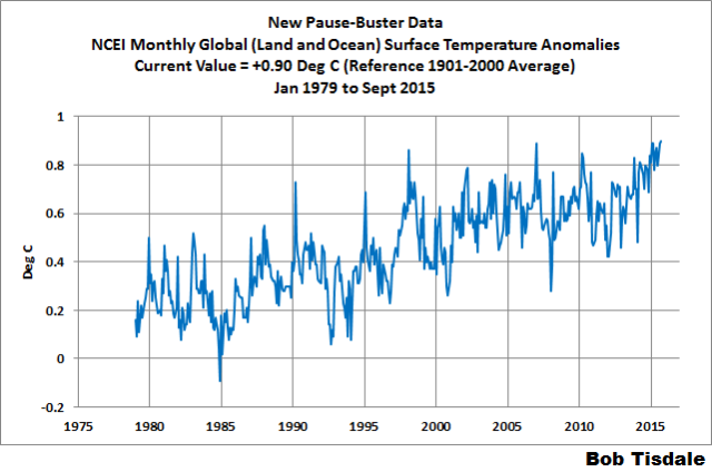
Figure 2 – NCEI Global (Land and Ocean) Surface Temperature Anomalies
UK MET OFFICE HADCRUT4 (LAGS ONE MONTH)
Introduction: The UK Met Office HADCRUT4 reconstruction merges CRUTEM4 land-surface air temperature product and the HadSST3 sea-surface temperature (SST) reconstruction. CRUTEM4 is the product of the combined efforts of the Met Office Hadley Centre and the Climatic Research Unit at the University of East Anglia. And HadSST3 is a product of the Hadley Centre. Unlike the GISS and NCEI reconstructions, grids without temperature samples for a given month are not infilled in the HADCRUT4 product. That is, if a 5-deg latitude by 5-deg longitude grid does not have a temperature anomaly value in a given month, it is left blank. Blank grids are indirectly assigned the average values for their respective hemispheres before the hemispheric values are merged. The HADCRUT4 reconstruction is described in the Morice et al (2012) paper here. The CRUTEM4 product is described in Jones et al (2012) here. And the HadSST3 reconstruction is presented in the 2-part Kennedy et al (2012) paper here and here. The UKMO uses the base years of 1961-1990 for anomalies. The monthly values of the HADCRUT4 product can be found here.
Update (Lags One Month): The September 2015 HADCRUT4 global temperature anomaly is +0.79 deg C. See Figure 3. It increased (about +0.05 deg C) since August 2015.

Figure 3 – HADCRUT4
UAH LOWER TROPOSPHERE TEMPERATURE ANOMALY COMPOSITE (UAH TLT)
Special sensors (microwave sounding units) aboard satellites have orbited the Earth since the late 1970s, allowing scientists to calculate the temperatures of the atmosphere at various heights above sea level (lower troposphere, mid troposphere, tropopause and lower stratosphere). The atmospheric temperature values are calculated from a series of satellites with overlapping operation periods, not from a single satellite. Because the atmospheric temperature products rely on numerous satellites, they are known as composites. The level nearest to the surface of the Earth is the lower troposphere. The lower troposphere temperature composite include the altitudes of zero to about 12,500 meters, but are most heavily weighted to the altitudes of less than 3000 meters. See the left-hand cell of the illustration here.
The monthly UAH lower troposphere temperature composite is the product of the Earth System Science Center of the University of Alabama in Huntsville (UAH). UAH provides the lower troposphere temperature anomalies broken down into numerous subsets. See the webpage here. The UAH lower troposphere temperature composite are supported by Christy et al. (2000) MSU Tropospheric Temperatures: Dataset Construction and Radiosonde Comparisons. Additionally, Dr. Roy Spencer of UAH presents at his blog the monthly UAH TLT anomaly updates a few days before the release at the UAH website. Those posts are also regularly cross posted at WattsUpWithThat. UAH uses the base years of 1981-2010 for anomalies. The UAH lower troposphere temperature product is for the latitudes of 85S to 85N, which represent more than 99% of the surface of the globe.
UAH recently released a beta version of Release 6.0 of their atmospheric temperature product. Those enhancements lowered the warming rates of their lower troposphere temperature anomalies. See Dr. Roy Spencer’s blog post Version 6.0 of the UAH Temperature Dataset Released: New LT Trend = +0.11 C/decade and my blog post New UAH Lower Troposphere Temperature Data Show No Global Warming for More Than 18 Years. The UAH lower troposphere anomalies Release 6.3 beta through October 2015 are here.
Update: The October 2015 UAH (Release 6.0 beta) lower troposphere temperature anomaly is +0.43 deg C. It rose (an increase of about +0.18 deg C) since September 2015.
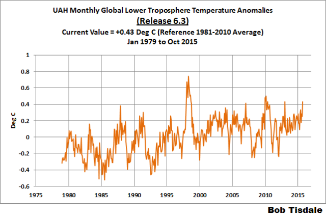
Figure 4 – UAH Lower Troposphere Temperature (TLT) Anomaly Composite – Release 6.3 Beta
RSS LOWER TROPOSPHERE TEMPERATURE ANOMALY COMPOSITE (RSS TLT)
Like the UAH lower troposphere temperature product, Remote Sensing Systems (RSS) calculates lower troposphere temperature anomalies from microwave sounding units aboard a series of NOAA satellites. RSS describes their product at the Upper Air Temperature webpage. The RSS product is supported by Mears and Wentz (2009) Construction of the Remote Sensing Systems V3.2 Atmospheric Temperature Records from the MSU and AMSU Microwave Sounders. RSS also presents their lower troposphere temperature composite in various subsets. The land+ocean TLT values are here. Curiously, on that webpage, RSS lists the composite as extending from 82.5S to 82.5N, while on their Upper Air Temperature webpage linked above, they state:
We do not provide monthly means poleward of 82.5 degrees (or south of 70S for TLT) due to difficulties in merging measurements in these regions.
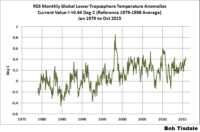
Also see the RSS MSU & AMSU Time Series Trend Browse Tool. RSS uses the base years of 1979 to 1998 for anomalies.
Update: The October 2015 RSS lower troposphere temperature anomaly is +0.44 deg C. It rose (an increase of about +0.07 deg C) since September 2015.
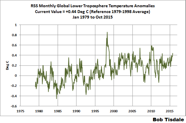
Figure 5 – RSS Lower Troposphere Temperature (TLT) Anomalies
COMPARISONS
The GISS, HADCRUT4 and NCEI global surface temperature anomalies and the RSS and UAH lower troposphere temperature anomalies are compared in the next three time-series graphs. Figure 6 compares the five global temperature anomaly products starting in 1979. Again, due to the timing of this post, the HADCRUT4 and NCEI updates lag the UAH, RSS and GISS products by a month. For those wanting a closer look at the more recent wiggles and trends, Figure 7 starts in 1998, which was the start year used by von Storch et al (2013) Can climate models explain the recent stagnation in global warming? They, of course, found that the CMIP3 (IPCC AR4) and CMIP5 (IPCC AR5) models could NOT explain the recent slowdown in warming, but that was before NOAA manufactured warming with their new ERSST.v4 reconstruction.
Figure 8 starts in 2001, which was the year Kevin Trenberth chose for the start of the warming slowdown in his RMS article Has Global Warming Stalled?
Because the suppliers all use different base years for calculating anomalies, I’ve referenced them to a common 30-year period: 1981 to 2010. Referring to their discussion under FAQ 9 here, according to NOAA:
This period is used in order to comply with a recommended World Meteorological Organization (WMO) Policy, which suggests using the latest decade for the 30-year average.
The impacts of the unjustifiable adjustments to the ERSST.v4 reconstruction are visible in the two shorter-term comparisons, Figures 7 and 8. That is, the short-term warming rates of the new NCEI and GISS reconstructions are noticeably higher during “the hiatus”, as are the trends of the newly revised HADCRUT product. See the June update for the trends before the adjustments. But the trends of the revised reconstructions still fall short of the modeled warming rates.

Figure 6 – Comparison Starting in 1979
#####

Figure 7 – Comparison Starting in 1998
#####
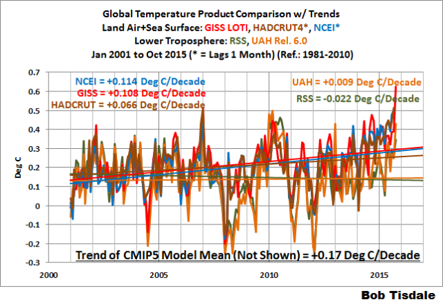
Figure 8 – Comparison Starting in 2001
Note also that the graphs list the trends of the CMIP5 multi-model mean (historic and RCP8.5 forcings), which are the climate models used by the IPCC for their 5th Assessment Report.
AVERAGES
Figure 9 presents the average of the GISS, HADCRUT and NCEI land plus sea surface temperature anomaly reconstructions and the average of the RSS and UAH lower troposphere temperature composites. Again because the HADCRUT4 and NCEI products lag one month in this update, the most current average only includes the GISS product.

Figure 9 – Average of Global Land+Sea Surface Temperature Anomaly Products
MODEL-DATA COMPARISON & DIFFERENCE
Note: The HADCRUT4 reconstruction is now used in this section. [End note.]
Considering the uptick in surface temperatures in 2014 (see the posts here and here), government agencies that supply global surface temperature products have been touting record high combined global land and ocean surface temperatures. Alarmists happily ignore the fact that it is easy to have record high global temperatures in the midst of a hiatus or slowdown in global warming, and they have been using the recent record highs to draw attention away from the growing difference between observed global surface temperatures and the IPCC climate model-based projections of them.
There are a number of ways to present how poorly climate models simulate global surface temperatures. Normally they are compared in a time-series graph. See the example in Figure 10. In that example, the UKMO HadCRUT4 land+ocean surface temperature reconstruction is compared to the multi-model mean of the climate models stored in the CMIP5 archive, which was used by the IPCC for their 5th Assessment Report. The reconstruction and model outputs have been smoothed with 61-month filters to reduce the monthly variations. Also, the anomalies for the reconstruction and model outputs have been referenced to the period of 1880 to 2013 so not to bias the results.

Figure 10
It’s very hard to overlook the fact that, over the past decade, climate models are simulating way too much warming and are diverging rapidly from reality.
Another way to show how poorly climate models perform is to subtract the observations-based reconstruction from the average of the model outputs (model mean). We first presented and discussed this method using global surface temperatures in absolute form. (See the post On the Elusive Absolute Global Mean Surface Temperature – A Model-Data Comparison.) The graph below shows a model-data difference using anomalies, where the data are represented by the UKMO HadCRUT4 land+ocean surface temperature product and the model simulations of global surface temperature are represented by the multi-model mean of the models stored in the CMIP5 archive. Like Figure 10, to assure that the base years used for anomalies did not bias the graph, the full term of the graph (1880 to 2013) was used as the reference period.
In this example, we’re illustrating the model-data differences in the monthly surface temperature anomalies. Also included in red is the difference smoothed with a 61-month running mean filter.
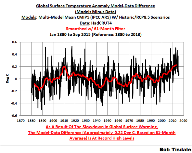
Figure 11
The greatest difference between models and reconstruction occurs now.
There was also a major difference, but of the opposite sign, in the late 1880s. That difference decreases drastically from the 1880s and switches signs by the 1910s. The reason: the models do not properly simulate the observed cooling that takes place at that time. Because the models failed to properly simulate the cooling from the 1880s to the 1910s, they also failed to properly simulate the warming that took place from the 1910s until 1940. That explains the long-term decrease in the difference during that period and the switching of signs in the difference once again. The difference cycles back and forth, nearing a zero difference in the 1980s and 90s, indicating the models are tracking observations better (relatively) during that period. And from the 1990s to present, because of the slowdown in warming, the difference has increased to greatest value ever…where the difference indicates the models are showing too much warming.
It’s very easy to see the recent record-high global surface temperatures have had a tiny impact on the difference between models and observations.
See the post On the Use of the Multi-Model Mean for a discussion of its use in model-data comparisons.
MONTHLY SEA SURFACE TEMPERATURE UPDATE
The most recent sea surface temperature update can be found here. The satellite-enhanced sea surface temperature composite (Reynolds OI.2) are presented in global, hemispheric and ocean-basin bases. We discussed the recent record-high global sea surface temperatures in 2014 and the reasons for them in the post On The Recent Record-High Global Sea Surface Temperatures – The Wheres and Whys.
NEW EBOOK

Just in case you haven’t encountered it, I recently published my new ebook On Global Warming and the Illusion of Control (25 MB .pdf). IT’S FREE. The post that introduces it is here (cross post at WattsUpWithThat is here).
Why arent the NCEP CFSv2 real time temperatures used. No adjustments, just the temp measured every 6 hours using what NCEP uses to initialize models. Anyone have anything against real time temps taken every 6 hours
Thanks, Joe Bastardi.
Where is a good, free access to NCEP CFSv2?
Weatherbell Analytics
I calculate an index based on NCEP/NCAR reanalysis here. It went up by 0.2°C from Sept to October, just a little less than GISS. And it also had October warmest month, by a long way.
There is some serious divergence between the databases going on again, it seems.
It’s to be expected that GISS, that looks at the surface, would warm more than the satellites that look in the troposphere.
El Nino releases heat from below (the Oceans).
The satellites are measuring warming in the atmosphere (the fingerprint of the AGW idea).
They aren’t the same thing.
The most striking thing to me is the difference between the data sets measured at the beginning of strong ENSO’s comparing 1998 to 2015. Maybe too early to draw conclusions but in 1998 GISS peaked within UAH/RSS. So far it looks like it will be reverse with GISS crowning UAH/RSS. Time will tell.
Should temperatures measured in UHI be reduced; after all they are an island? Where I live, driving into town always shows a +4 F to +9 F increase from the surrounding area which is primarily covered in trees rather than airport concrete and asphalt. Airport temps are only useful to aircraft performance.
But the objective of climate “science” is to show the greatest possible (or even impossible) temperature increase. They need to “adjust” those rural temps to match those city temps. Pronto!
I’ll be spending my week at the ranch covered with snow (I know just weather) …it will give me an opportunity to read Bob’s excellent work.
Amazing. I distinctly remember that one of the reasons GISS had 2005 hotter than 1998 is they claimed GISS didn’t see all the heat the satellites did in 1998 and therefore had it cooler. Now the NINO3.4 temps are similar, they show a huge spike in temp. They really are having their cake and eating it too.
Thanks, Bob.
This is a good way to follow the effects of the ongoing El Niño.
NOAA-NWS Climate Prediction Center – CPC thinks “El Niño will likely peak during the Northern Hemisphere winter 2015-16, with a transition to ENSO-neutral anticipated during the late spring or early summer 2016.”
See http://www.cpc.ncep.noaa.gov/products/analysis_monitoring/enso_disc_nov2015/ensodisc.html
The Mark 1 eyeball detects that there is a drop in the variability of the 4 surface temperature indices (Fig 1 thru 4) during The Pause. Which suggests climate change is making temperature less variable and thus less extreme.
Either that or the Pause Buster adjustments are affecting the variability of the data.
The GISS anomaly for October at 104 smashed the previous all time mark of 97 from January 2007.
However with RSS, its October value of 0.440 was beaten in 1998 at 0.461. Furthermore, all of the first 10 months of 1998 beat 0.440.
UAH6.0beta3 did have its highest October on record at 0.427. However all of the first 9 months of 1998 beat that mark.
Werner Brozek
November 16
“UAH6.0beta3 did have its highest October on record at 0.427. However all of the first 9 months of 1998 beat that mark.”
________________
That’s true, but the 1998 temperatures were reflecting the later stages of the 1997/98 El Nino, which began in spring 1997 and peaked in late fall/early winter the same year. The satellite data typically lags the El Nino warming by around 6 months, hence the very high early-mid 1998 lower troposphere temperatures.
The current El Nino only began this spring, going by the NOAA index, and it has yet to peak. The October spike in LT temperatures reflects a surge in ENSO3.4 SST warming that began several months ago. If the current El Nino peaks in December, then it’s unlikely we’ll see the LT peak before mid 2016.
It’s likely that satellite-derived lower troposphere temperatures will remain high and perhaps continue to rise on average over the next 6-8 months. We could well see the 1998 record beaten in 2016.
That is certainly possible and cannot be ruled out. But 2015 cannot even reach second place.
I do not know how good channel 6 is at predicting the final result. I wish it were better. However it seems very clear that the November anomaly will be way lower than that of 2014 if their plots give a good indication. As for beating 1998 or even 2010, that clearly cannot happen any more. Even if there should be a huge spike in November and December, there simply are not enough months left to even get to second place.
It would have to average 0.84 over the next two months to reach second. The all time record for UAH is 0.742.
I agree that it’s very unlikely that 2015 will set any new satellite temperature records.
As I said though, we’re much more likely to see a new satellite temperature record set in 2016, given the lag between ENSO3.4 and lower troposphere temperature increase.
what i find odd is how suddenly this el nino the rise of GISS precedes the satellite rise instead of lagging it.
to me that’s odd…. any thought on that?
GISS appears to be an attempt to get a global land+ocean surface temperature.
The RSS numbers are for the lower troposphere.
The lower troposphere is partially heated by the surface – with a lag.
Have I missed something in you question?
See this comparison of data sets, by Bob T.
Link here.
“The lower troposphere responds to the change in surface temperature of the tropical Pacific but mostly to the changes in evaporation from the tropical Pacific. For example, during an El Niño, the sea surfaces of the eastern tropical Pacific warm. This also results in an increase in evaporation. Warmer water yields more evaporation. As the warm, moist air rises, it cools and condenses, releasing additional heat to the atmosphere.”
That’s just under Figure 10 in the linked to post.
Surface temperatures typically lag El Nino (and La Nina) peas and troughs by ~3 months. Satellite (lower troposphere) temperatures typically lag by ~ 6 months.
We won’t see a peak in satellite temperatures until spring 2016.
Totally hilarious to see grown men (and women) discussing whether the PLANET has warmed by 0.2 of a degree or whether it has warmed by 0.18 of a degree C!
I am very much reminded of the famous 19th century Anglican theologians who disputed the number of angels that might dance on the head of a pin.
The angels-on-the-head-of-a-pin story appears to be apocryphal, not to mention attributed to different sources in a different period. See https://en.wikipedia.org/wiki/How_many_angels_can_dance_on_the_head_of_a_pin%3F
Perhaps Jonathon Swift’s account in Gulliver’s Travels of a project, at the grand academy of Lagado, to extract sunbeams from cucumbers might be more apt comparison?
The number is apparently open for debate, depending upon the agility of the angels. http://sundaycomic.smackjeeves.com/comics/1166973/enquiring-minds-want-to-know/
It is not at all hilarious. Remember, Billions of our ( and some of your) dollars are being WASTED on this!
Reminds me of an editor I once worked for in Business News at a Texas daily who averaged the growth-rate projections of eight local economists to two decimal places — for greater accuracy.
How anybody can publish anything serious about GISS, hadcrut ect surface temperatures is beyond me. Their data has been shown to be 100% doctored refer to Paul Homewood, Goddard, even here ect…
If we accept temperature anomaly estimates are correct, we face an unresolved enigma.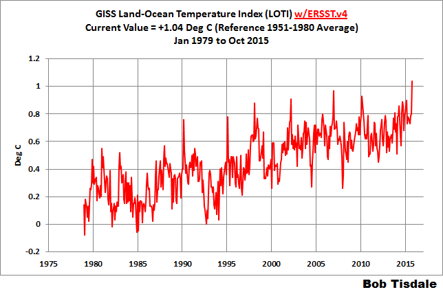
As you can see, rate of warming at the surface is much higher, than in the lower troposphere. That means global average lapse rate is increasing. As moist lapse rate is much lower than dry one, it means the troposphere is getting drier, otherwise environmental lapse rate could not increase. However, the surface is warming, and that means more evaporation, which makes the troposphere more humid, not less. These two sentences are clearly inconsistent, so either one of them is false or both.
The theory and the global warming models actually predict the opposite to occur.
The lower troposphere is supposed to warm at a rate 30% higher than the surface, not 50% lower. And the lapse rate is supposed to increase, not decrease.
So, either the surface records are being drastically distorted or the models have to be re-written. At some point, this will come to a head.
I think, generally, everyone on the pro-side and the skeptic side of this debate, now understand that the surface records are not reliable anymore. Tom Karl has distorted the trend by about 50% and he will go down as one of the worst, most impact, data distorters of all time. Someone can start the Wiki page right now.
Read more @ http://joannenova.com.au/
Article title: “Blockbuster: Are hot days in Australia mostly due to low rainfall, and electronic thermometers — not CO2?”
The ECMWF’s ERA-interim reanalysis product also has October as the “warmest month ever”, but still, it has been more or less flat since about 2001: http://climate.copernicus.eu/resources/data-analysis/average-surface-air-temperature-analysis/monthly-maps/october-2015
The warmists will flog ie promote this posting to no end. its gives credibility to GISS ect
NOAA claims a largest ever 3K anomaly for the el nino. Could they have some bias in the anomaly calculation like for land temperature?
It would be nice with other measurements of sea temperature, e.g. from satellites.
“Svend Ferdinandsen
November 17, 2015 at 4:02 am
Could they have some bias in the anomaly calculation…”
Therein LIES the problem. No measurements just calculations. Math(s). Averages. Statistics. Anomalies.
Bob Tisdale: Can you wait a couple of days to include NOAA/NCEI data? The schedule is posted at https://www.ncdc.noaa.gov/monitoring-references/dyk/monthly-releases although they do have some last-minute delays. Their October global data is due tomorrow. The download procedure is 100% manual. Go to webpage…
https://www.ncdc.noaa.gov/monitoring-references/faq/anomalies.php
Click on… “Anomalies and Index Data”, and click on the blue “Download” button. The default values “Monthly”, “Global”, “Land and Ocean”, and “CSV” are the correct values for what you want. You’ll get a text page of numbers. In your web browser, save the page as a text file.