This is a guest essay by Mike Jonas, part 1 of 4
Introduction
The aim of this article is to provide simple mathematical formulae that can be used to calculate the carbon dioxide (CO2) contribution to global temperature change, as represented in the computer climate models.
This article is the first in a series of four articles. Its purpose is to establish and verify the formulae, so unfortunately it is quite long and there’s a fair amount of maths in it. Parts 2 and 3 simply apply the formulae established in Part 1, and hopefully will be a lot easier to follow. Part 4 enters into further discussion. All workings and data are supplied in spreadsheets. In fact one aim is to allow users to play with the formulae in the spreadsheets.
Please note : In this article, all temperatures referred to are deg C anomalies unless otherwise stated.
Global Temperature Prediction
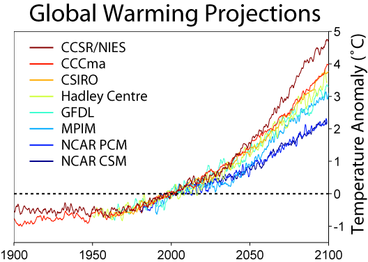
The climate model predictions of global temperature show on average a very slightly accelerating increase between +2 and +5 deg C by 2100:

We can be confident that all of this predicted temperature increase in the models is caused by CO2, because Skeptical Science (SkS) [6], following a discussion of CO2 radiative forcing, says :
Humans cause numerous other radiative forcings, both positive (e.g. other greenhouse gases) and negative (e.g. sulfate aerosols which block sunlight). Fortunately, the negative and positive forcings are roughly equal and cancel each other out, and the natural forcings over the past half century have also been approximately zero (Meehl 2004), so the radiative forcing from CO2 alone gives us a good estimate as to how much we expect to see the Earth’s surface temperature change.
[my emphasis]
So, if we can identify how much of the global temperature change over the years from 1850 to present was contributed by CO2, then we can deduce how much of the temperature change was not. ie,
T = Tc + Tn
where
T is temperature.
Tc is the cumulative net contribution to temperature from CO2. “CO2” refers to all CO2, there is no distinction between man-made and natural CO2.
Tn is the non-CO2 temperature contribution.
Obviously, all feedbacks to CO2 warming (changes which occur because the CO2 warmed) must be included in Tc.
CO2 Data
The Denning Research Group [4] helpfully provide an emissions calculator, which shows CO2 levels and the estimated future temperature change that it causes under “Business as usual” (zero emission cuts) :

Cross-checking the future warming in this graph against Figure 1, the CO2 warming from 2020-2100 is just under 3.5 deg C compared with about 3.25 deg C model average in Figure 1. That seems close enough for reliable use here. But data going back to at least 1850 is still needed.
There is World Resources Institute (WRI) CO2 data from 1750 to present [3], and CO2 data measured at Mauna Loa from 1960 to present [5]. Together with the Denning “Business as usual” CO2 predictions above, the CO2 concentration from 1750 to 2100 is as follows :

For dates covered by more than one series, the Mauna Loa measured data will be preferred, then the WRI data.
Because the “pre-industrial” CO2 is put at 280ppm [6], and the data points in the above graph before 1800 are all very close to 280ppm, a constant level of 280ppm will be assumed before 1800.
CO2 Contribution
The only information still needed is the CO2-caused warming before about 1990.
A method for calculating the temperature contribution by CO2 is given by SkS in [6] :
dF = 5.35 ln(C/Co)
Where ‘dF’ is the radiative forcing in Watts per square meter, ‘C’ is the concentration of atmospheric CO2, and ‘Co’ is the reference CO2 concentration. Normally the value of Co is chosen at the pre-industrial concentration of 280 ppmv.
dT = λ*dF
Where ‘dT’ is the change in the Earth’s average surface temperature, ‘λ’ is the climate sensitivity, usually with units in Kelvin or degrees Celsius per Watts per square meter (°C/[W/m2]), and ‘dF’ is the radiative forcing.
So now to calculate the change in temperature, we just need to know the climate sensitivity. Studies have given a possible range of values of 2-4.5°C warming for a doubling of CO2 (IPCC 2007). Using these values it’s a simple task to put the climate sensitivity into the units we need, using the formulas above:
λ = dT/dF = dT/(5.35 * ln[2])= [2 to 4.5°C]/3.7 = 0.54 to 1.2°C/(W/m2)
Using this range of possible climate sensitivity values, we can plug λ into the formulas above and calculate the expected temperature change. The atmospheric CO2 concentration as of 2010 is about 390 ppmv. This gives us the value for ‘C’, and for ‘Co’ we’ll use the pre-industrial value of 280 ppmv.
dT = λ*dF = λ * 5.35 * ln(390/280) = 1.8 * λ
Plugging in our possible climate sensitivity values, this gives us an expected surface temperature change of about 1–2.2°C of global warming, with a most likely value of 1.4°C. However, this tells us the equilibrium temperature. In reality it takes a long time to heat up the oceans due to their thermal inertia. For this reason there is currently a planetary energy imbalance, and the surface has only warmed about 0.8°C. In other words, even if we were to immediately stop adding CO2 to the atmosphere, the planet would warm another ~0.6°C until it reached this new equilibrium state (confirmed by Hansen 2005). This is referred to as the ‘warming in the pipeline’.
Unfortunately, not enough exact parameters are given to allow the temperature contribution by CO2 to be calculated completely, because the effect of ocean thermal inertia has not been fully quantified. But it should be reasonable to derive the actual CO2 contribution by fitting the above formulae to the known data and to the climate model predictions.
The net radiation caused by CO2 is the downward infra-red radiation (IR) as described by SkS, less the upward IR from the CO2 warming already in the system (CWIS). This upward IR will be proportional to the fourth power of the absolute (deg K) value of CWIS [9]. The net effect of CO2 on IR is therefore given by :
Rcy = 5.35 * ln(Cy/C0) – j * ((T0+Tcy-1)^4 – T0^4)
where
Rcy is the net downward IR from CO2 in year y.
Cy is the ppm CO2 concentration (C) in year y.
C0 is the pre-industrial CO2 concentration, ie. 280ppm.
j is a factor to be determined.
T0 is the base temperature (deg K) associated with C0.
Tcy is the cumulative CO2 contribution to temperature (Tc) at end year y, ie, CWIS.
SkS [6] says “it takes a long time to heat up the oceans due to their thermal inertia”. On this basis, CWIS is presumably in some ocean upper layer.
For a doubling of CO2, in the absence of other natural factors, the equilibrium temperature increase using the SkS formula is 5.35 * ln(2) * λ where λ = 3.2/3.7 (assuming a mid-range equilibrium climate sensitivity (ECS) of 3.2).
At equilibrium, Rc = 0. For ECS = 3.2, j can therefore be determined from
0 = 5.35 * ln(2) – j * ((T0+3.2)^4 – T0^4)
hence
j = (5.35 * ln(2)) / ((T0+3.2)^4 – T0^4)
Because “the natural forcings over the past half century have also been approximately zero” [6], the SST should be a reasonably good guide to CWIS. The global average SST 1981 to 2006 was 291.76 deg K [8]. Subtracting the year 1993 Tc of 0.7 (from the Denning data [4]) gives T0=291 deg K. Hence j = (5.35 * ln(2)) / ((291+3.2)^4 – 291^4) = 1.16E-8 (ie. 1.16 * 10^-8, or 0.0000000116).
Using the formula
δTcy = k * Rcy
where
δTcy is the increase (deg C) in CWIS in year y.
k is the one-year impact on temperature per unit of net downward IR.
the value of k can be found which gives a future temperature increase matching that of the climate models, ie. 3.25 deg C from 2020 to 2100. A reasonability check is that the result should closely match but be slightly lower than the Denning warming calculation in Figure 2 (lower graph) (slightly lower because target is 3.25 deg C not 3.5) …..

….. it does, for k = 0.02611 (the graph for 3.5 deg C is also shown in [7]). [Note that the calculated warming is “anchored” at 1750 T=0, and that the shape is determined only by the formula so there is no guarantee that the 2020 and 2100 temperatures will be close to the Denning temperatures. ie, this is a genuine test.].
Note: At this rate, global temperature takes 52 years to get 80% of the way to equilibrium (as in “equilibrium climate sensitivity”), 75 years to reach 90%, 97 years to reach 95%, 148 years to reach 99%.
The above formula can therefore reliably be used for CO2’s contribution to global temperature since 1750.
1850 to 2100
The above formulae can now be applied to the period 1850 – 2100, to see how much has been and will be contributed to temperature by CO2.
For temperature data 1850 to present, Hadcrut4 global temperature [1] is used. For future temperatures, the formula warming (as in Figure 4) is used.

Applying the above formulae shows the contributions to temperature by CO2 and by other factors :

As expected,
· the dominant contribution is from CO2,
· other factors contribute the inter-annual “wiggles” and virtually nothing else.
Note : The contribution to global temperature by CO2 is only man-made to the extent that the CO2 is man-made. As stated earlier, no distinction is made between man-made CO2 and natural CO2. Obviously, all pre-industrial CO2 was in fact natural. Similarly, for the non-CO2 contribution, no distinction is made between natural factors and non-CO2 man-made factors (such as land-clearing, for example), but the non-CO2 factors are thought to be predominantly natural. The feedbacks from the CO2 warming as claimed by the IPCC (eg. water vapour, clouds) are included in the CO2 contribution above.
Conclusion
The picture of global temperature and its drivers as presented by the IPCC and the computer models is one in which CO2 has been the dominant factor since the start of the industrial age, and natural factors have had minimal impact.
This picture is endorsed by organisations such as SkS and Denning. Using formulae derived from SkS, Denning and normal physics, this picture is now represented here using simple mathematical formulae that can be incorporated into a normal spreadsheet.
Anyone with access to a spreadsheet will be able to work with these formulae. It has been demonstrated above that the picture they paint is a reasonable representation of the CO2 calculations in the computer models.
The next articles in this series will look at applications of these formulae.
Footnote
It is important to recognise that the formulae used here represent the internal workings of the climate models. There is no “climate denial” here, because the whole series of articles is based on the premise that the climate computer models are correct, using the mid-range ECS of 3.2.
See spreadsheet “Part1” [7] for the above calculations.
Mike Jonas (MA Maths Oxford UK) retired some years ago after nearly 40 years in I.T.
References
[1] Hadley Centre Hadcrut4 Global Temperature data http://www.metoffice.gov.uk/hadobs/hadcrut4/data/current/time_series/HadCRUT.4.3.0.0.annual_ns_avg.txt (Downloaded 20/5/2015)
[2] Climate model predictions from http://upload.wikimedia.org/wikipedia/commons/a/aa/Global_Warming_Predictions.png (Downloaded 20/5/2015) Note: Wikipedia is an unreliable source for contentious issues, but for factual information such as the output of computer models, and in the context for which it is being used here, it should be OK.
[3] CO2 data from 1750 to date is from World Resources Institute http://powerpoints.wri.org/climate/sld001.htm (Downloaded 20/5/2015. Digitised using xyExtract v5.1 (2011) by Wilton P Silva)
[4] Emissions calculator from Denning Research Group at Colorado State University http://biocycle.atmos.colostate.edu/shiny/emissions/ using no emissions cuts, ie, “Business as usual”. (Downloaded 20/5/2015. Digitised using xyExtract v5.1 (2011) by Wilton P Silva)
[5] Mauna Loa CO2 data from http://scrippsco2.ucsd.edu/data/flask_co2_and_isotopic/monthly_co2/monthly_mlf.csv (Downloaded 27/2/2012)
[6] Skeptical Science 3 Sep 2010 http://www.skepticalscience.com/Quantifying-the-human-contribution-to-global-warming.html (As accessed 20/5/2012).
[7] Spreadsheet “Part1” with all data and workings . Part1 (Excel .xlsx spreadsheet)
[8] Spreadsheet “SST” SST (Excel .xlsx spreadsheet)
[9] Stefan-Boltzmann law. See http://hyperphysics.phy-astr.gsu.edu/hbase/thermo/stefan.html
Abbreviations
AR4 – (Fourth IPCC report)
AR5 – (Fifth IPCC report)
CO2 – Carbon Dioxide
CWIS – CO2 warming already in the system
ECS – Equilibrium Climate Sensitivity
IPCC – Intergovernmental Panel on Climate Change
IR – Infra-red (Radiation)
LIA – Little Ice Age
MWP – Medieval Warming Period
SKS – Skeptical Science (skepticalscience.com)
WRI – World Resources Institute
“We can be confident that all of this predicted temperature increase in the models is caused by CO2, because Skeptical Science (SkS) [6], following a discussion of CO2 radiative forcing, says :
Wrong.
You are looking at both history and future projections.
If you want to know what FORCINGS drove the model, you cannot and should not rely on SKs
GO TO THE SOURCE.
The forcing files are available for all CMIP experiements.. THAT is the proper source. not Sks.
science 101.. Primary sources. USE THEM.
Hi Steven – Everything cross-checks. The mid-range models exactly match the predictions from the mid-range ECS on their own. Bar a few small wiggles, the past 150 years of actual temperatures exactly match the application of the mid-range ECS on its own (Figure 6). In other words, the past and the future both match exactly the supposed effects of CO2, assuming the mid-range ECS, plus nothing else. The forcings you talk about are all built into this process, IOW they are all built into the ECS. By using the ECS, I am in fact using them.
Which means these effects (presumed to be anthropogenic in origin) fall within natural variability …as best as one can calculate.
Mike: FWIW, I don’t trust SKS to accurately report consensus climate science, so it will be difficult to trust your derivative work. I agree with Mosher, go to the original sources.
You are using a formula with values derived from the assumption that all observed warming is from CO2. That means the results will absolutely match all data that went into the calculation of that value.
It is similar to tricks used to compress image data in a “lossy” manner.
Depending on when you calculated the ECS value you can get different expected curves that will fit the past data and, due to the dependence of future temps on current and past temps, be reasonably assured of a trend that will appear to fit for at least a couple of decades.
I’m also not convinced that there aren’t naturally sources of warming. 20th century solar activity, alone, was quite different than from the 19th century, and no one really agrees on what the effects would have been (more/less cloud nucleation? more/less wind? altered wind/ocean currents? etc…).
And, of course, the other data assumption is the CO2 levels themselves, but there is little we can do about that.
[snip]
[ Until you start providing links and description, you don’t get to simply yell WRONG here anymore. Step up – Anthony]
It depends on what the author’s purpose is, which we do not yet know (at least I don’t, since make no clairvoyancy claims). Lewis and Curry (2014) used central AR5 values (even though several have since been ‘improved’ ) to show that the likeliest ECS must be at the low end of the stated AR5 range. A rather nice ‘Perry Mason’ paper sticking it to AR5, yet also criticized for not using the newest estimates–which would have defeated the purpose. Maybe this is similar, in which case your point is not just irrelevant, but also wrong. Why not have the patience to find out what the purpose here is?
Sketchy Science is what the shill site “Skeptical science” does. It poses as realist, but is actually designed to twist the real science that disproves the Global Warming Claims and make it look stupid or impotent. Find the real thing at WattsUpWith That.com
So many assumptions, so little time. In the end, reality shows it is wrong.
Yeah, Bruce, i don’t spend too much time here at watts, but i must say this is the most delusional posting that i’ve seen here in a long while. I do wish anthony would be more careful about what’s being posted here…
Guys, get a grip. This is establishing what the SkS models say. It’s not saying those models are right.
Agreed, the physics of a specific glibal ti Co2 interaction aught to be well understood by now, its what is not well understood which intrigues the most. There could be dozens of interactions which are not well understood driving climate in spite of C02 forcing. And we may have physics revise the math behind the radiative properties of C02 before long.
Well done looking forward to the series.
So the question becomes what is ECS value? If doubling CO2 will give us 1-1.7 C increase in temperature how do they get to 3.2? Feedbacks? Which ones and where is the data?
Thanks for the article. I’m looking forward to the next 3 parts.
I have strong objections on labeling the RCP8.5 scenario as “business as usual”. RCP8.5 is a worst case scenario similar to SRES A1FI. Using the real busines as usual model SRES A1B with a climate sentitivity of 1.3 yields this: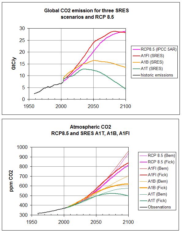
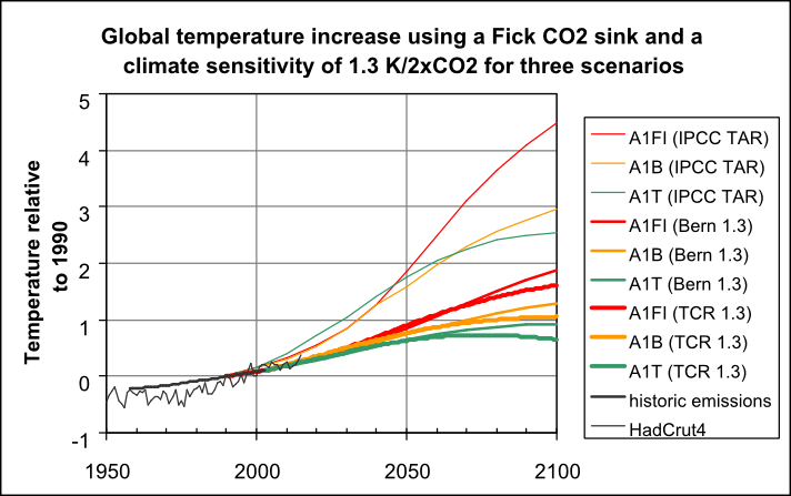
With this temperature calculation:
So only a one degree rise after 1990
Hans Erren,
You are absolutely right. RCP8.5 is a fantasy. The path we are on will take us somewhere between RCP4.5 and RCP6, unless there are breakthroughs in non-fossil energy (as, of course, there will be).
RCP8.5 isn’t a fantasy, it is a scenario based on clear assumptions, no more no less. It doesn’t claim to forecast what might or mightn’t happen, it is a projection that “corresponds to a high greenhouse gas emissions pathway compared to the scenario literature .., and hence also to the upper bound of the RCPs”.
HAS, all scenarios are science fiction the underlying assumption of A2 is increasing poverty combined with extreme population growth. That’s not business as usual for India nor China.
Hans
You miss my point.
The scenarios are no more than the product of their assumptions. Discuss the assumptions and the ways they have been projected into the future by all means, but don’t expect them to give a realistic view of the future unless the assumptions align with what is happening and the methods of projection valid (which as you note they don’t).
The point of criticism is the people that take the scenario and ascribe to it more meaning than it has – claiming for it a realistic view of the future usually under cover of calling RCP8.5 “business as usual”.
I should add that that follows through to the GCMs that are again basically complex projections rather than forecasts, and the RCPs are just one of the assumptions made to form those projections.
GCMs only become problematic when people start saying that their output is the way the world will be (and suggesting their range of outputs are “likely” for example as AR5 WG1 did).
But as you know CO2 can’t produce warming can it! And most of the CO2 came from warming oceans and that has stopped!
Sorry to post off topic, but everyone has to read this. That man Wadhams has completely lost it now!
http://www.telegraph.co.uk/news/earth/environment/globalwarming/11762680/Three-scientists-investigating-melting-Arctic-ice-may-have-been-assassinated-professor-claims.html
And yet, the alarmists are known to continually accuse “climate deniers” of adhering to conspiracy theories.
Micheal Mann’s depression deepened on reading this. He especially felt low about the report on the lady who was in the house when that one guy fell down the stairs claiming that homicide was preposterous. But back to the math at hand!
Also in The Times today, there is an article on the NOAA claim that this is the going to be the hottest year on record, referencing Mann’s latest paper in which he claims we are all going to hell in a hand cart, even with a two degree temperature rise. At that temperature, Mann et al claim a sea level rise of 10ft in 50 years. They also state that CO2 is a ‘tight control knob on global climate’, but they are not claiming that Big Oil is trying to assassinate them, so I guess that they haven’t totally flipped (yet).
I’m dealing with second hand information, so it’s hard to tell how accurate, but according to accounts Giles ran into a small delivery truck, the truck did not run into her. Laxon fell down a flight of stairs at a New Years party and died of a brain hemorrhage.
If this was murder then this is the most clever and skilled assassin in history to have multiple cases where the victim initiates the final sequence leading to death.
They are super ninja turbo charged oil fed murdering assassins that use vulcan mind meld to steer their victims to their demise! They throw Neon bright spinney star like thoughts of death right out of their foreheads!
Easy. Just spike the drinks with heavily magnetized rare earth metals. Person runs into truck because its largely metal. Person falls down stairs because a strange delivery consisting of a blob of metal was left at the bottom of steep stairs. Man struck by lightning because of the metal inside him. I totally buy this (sarc).
In fairness he has a point.
Nobody ever has an accident on a bicycle without there being nefarious causes.
Motorway bumps are unheard of ever. And he probably would have died if he hadn’t had that covert advanced automobile training with MI6 (shh).
And the guy who was hit by lightning was clearly attacked with a CIA/Exxon space Tesla Ray.
Lewandowsky can explain why you’re being irrational in doubting the great scientist.
Arranging for someone to be struck by lightning is a neat trick. Who would ever suspect it was murder?
It just shows that the conspiracy goes right to the top.
Interesting, but unlikely to be a coincidence.
There may be an important common element, which I am very familiar with.
I often come across something in a data file, and however unlikely when it confirms my expectations, I wander down the road oblivious of the surroundings, unable to get it out of my head until I can glimpse some kind of resolution.
These scientists died in early months of 2013, while Arctic Sea ice extent in the late 2012 hit new low.
http://ocean.dmi.dk/arctic/plots/icecover/icecover_current_new.png
All three were very intelligent highly educated people, I suspect they knew perfectly well that this could not have been consequence of the CO2; but what is it and why?
Lack of concentration while riding a bike even for few seconds in London traffic, or coming down stairs (I did it once, had bruised ‘lower back’ for months, my wife see only funny side of it). Going to a UK hospital on Sunday, let alone New Years day with a life threatening injury, a very slim chance of recovery. In the third case could be simply carelessness and ignorance of the elements by walking in a thunderstorm while the mind is preoccupied by some other matter.
Professor Peter Wadhams you are wrong, not succession of assassinations, as your own case confirms. Of course you wouldn’t be also loosing concentration while driving and daydreaming about “ that the North Pole will be exposed (no ice) this summer – it’s not happened before” as you claimed some years ago, or some other nonsense, but for some reason a crazy lorry driver didn’t like your climate politics.
It is entertaining to see so much math, when some of the underlying initial assumptions are completely fabricated. I have seen nothing which would indicate that carbon dioxide was a specific steady-state level from 1750 to about 1900. The published numbers from that time were all over the place, depending on where the air samples were taken. The numbers being used here are taken from the lowest readings, and are not even an average from known readings in a general area. This would be interesting if it was based upon some real numbers as a starting point.
Janice,
The old (chemical) measurements were more or less reliable (+/- 10 ppmv with good skills), the places where they were taken were not: midst of towns, under, in between and over growing crops, midst of forests, etc… Completely unreliable for “background” CO2 levels.
The 280 ppmv is mainly taken from the most uncontaminated places (over the oceans, coastal with wind from the sea) and are around the ice core data which have a resolution of around 20 years over the past 1,000 years.
Looking forward to part 4 but stopped reading whe you quoted the Skeptical Science rag. Please find more credible sources to establish the math.
Also, the assumption that co2 alone will cause a linear change in the climate system is nonsense and the reason the models are so flawed/inaccurate.
Looking forward to part 4 but stopped reading whe you quoted the Skeptical Science rag
Patience young Paduan, the purpose is likely to hoist them on their own petard.
exactly my thought. Let’s wait to see where he takes this before commenting.
Peter,
I think you are correct in your prediction.
Sorry to be pedantic, but I believe it would be “to hoist them [with/by] their own petard”. I believe a petard is a bomb, in medieval times affixed to a gate to blow a hole for getting into a fortification. The quote comes from Shakespeare (Hamlet) and I believe means “blown up by one’s own bomb”.
Exactly. Once we confirm he’s on our side, we’ll be able to accept the science. Otherwise, it will be summarily dismissed.
Yeah, John, this is really a bit bizarre of jonas… The warming of a hundred years ago is thought to be largely natural as well as up to half of recent warming (if that’s even to be believed). So nearly three quarters of the warming is due to nature alone. Maybe i’m not understanding the point that jonas is trying to make (?)…
John. Sorry if I didn’t make it clear – I’m establishing the maths used in the climate models, and to do that I’m uncritically using the logic behind the climate models. I then apply the maths later in the series.
Hi Mike,
IMO, SKs is not nor is it ever likely to be considered a credible source. Its credibility has been undermined by the antics of its principals. I was simply pointing out my reaction.
Looking forward to Part 4.
“It is important to recognise that the formulae used here represent the internal workings of the climate models. There is no “climate denial” here, because the whole series of articles is based on the premise that the climate computer models are correct, using the mid-range ECS of 3.2.”
Well, unfortunately “the premise that the climate computer models are correct” is false for many reasons, thus rendering the remainder of this article incorrect. Reasons include, but are not limited to,
1. An artificially fixed tropospheric lapse rate of 6.5K/km, which does not adjust to perturbations in the atmosphere. This false assumption artificially limits negative lapse rate feedback convection. Using physically correct assumptions, Kimoto (link below) finds the climate sensitivity to doubled CO2 to be a negligible 0.1-0.2C.
2. Mathematical error in the calculation of the Planck response parameter λ, due to a false assumption of fixed emissivity, an error which continues to be promulgated by the IPCC (explained in section 3 of this Kimoto paper):
http://hockeyschtick.blogspot.com/2015/07/collapse-of-agw-theory-of-ipcc-most.html
3. Positive feedback from water vapor (whereas millions of radiosonde & satellite observations demonstrate water vapor has a net negative-feedback cooling effect)
4. Fixed relative humidity (contradicted by observations showing a decline of mid-troposphere relative and specific humidity) (A new paper also finds specific humidity is the most non-linear and non-Gaussian variable in weather models, also implying relative humidity is non-linear, and borne out by observations)
5. Neglect of the < 15 micron ocean penetration depth of GHG IR radiation, which greatly limits potential greenhouse gas warming of the top ocean layer.
6. Incorrect assumption that line-emitters CO2 and H2O are blackbodies for which Planck's, Kirchhoff's, & Stefan-Boltzmann laws apply [your equation [9] above]. Neither are blackbodies, don't have a Planck curve, and their emissivity decreases with temperature, *opposite* to a true blackbody.
7. False assumption that CO2 can absorb/emit at an equivalent blackbody temperature of anywhere from 200K-330K (but is limited to ~15 micron line-emission emitting temperature of 193K maximum by basic physical chemistry & quantum theory).
et al
Clarification above on #6: “…their emissivity decreases with increased temperature, *opposite* to a true blackbody.”
Hockeyschtick
The emissivity of a blackbody is 1.00. I cannot, by definition, increase with temperature. It is already a perfect emitter.
Did you mean something else?
The emissivity of most things is surprisingly constant with temperature provided it doesn’t start burning.
“The emissivity of a blackbody is 1.00”
Correct, but the points I was trying to make are that CO2 and H2O are mere line-emitters and not true blackbodies, emissivity is always less than a true blackbody, i.e. 193K.
For some reason, the remainder of my reply got cut off:
CO2 & H2O are mere line-emitters and not true blackbodies for which emissivity = 1. GHGs have emissivities 193K.
GHGs CO2 & H2O are mere line-emitters and not true blackbodies for which emissivity = 1. GHGs have emissivities 193K.
Mod: for some reason your system has repeatedly cut off the remainder of my comment I’ve tried to post 4 times – I think I discovered problem using a less than sign w/o a space… Trying one more time:
GHGs CO2 & H2O are mere line-emitters and not true blackbodies for which emissivity = 1. GHGs have emissivities less than 1 like true blackbodies and which decline further with temperature as proven by observations:
The reason why is basic physical chem & quantum theory. For example, for CO2 ~15 micron line-emission, the maximum possible emitting temperature is 193K by Planck’s/Wein’s Laws. 193K CO2 photons cannot transfer heat or be thermalized/warm any body at more than 193K.
http://hockeyschtick.blogspot.com/search?q=kirchhoff+planck
hockeyschtick ,
There is much to criticize in climate models, but these claims are bogus. No more than two of 1, 3, and 4 can be true. And none of this claims are consistent with what is actually done in climate models.
There is much to criticize in climate models, but these claims are bogus. No more than two of 1, 3, and 4 can be true.
It only takes one being true to falsify the models. I think taking a shotgun approach and then eliminating the incorrect ones by scientific method is a reasonable approach. Thanks for suggesting which candidates to target first.
“but these claims are bogus… And none of this claims are consistent with what is actually done in climate models”
Absolutely false. If you had bothered to read and understand the Kimoto papers
http://hockeyschtick.blogspot.com/2015/07/collapse-of-agw-theory-of-ipcc-most.html
you will find the literature citations which show the Hansen/NASA/GISS & IPCC models do in fact make these false assumptions. The 1976 US Std Atmosphere also proves many of these same false assumptions, and did not use one single radiative transfer calculation in their mathematical model of the temperature profile from 0-100km.
Arguments solely from the authority of “Mike M.” are worthless without out any specifics or references/mathematics/links/etc to back them up.
Kimoto’s paper is bad. But if you had bothered to read it, you would find that he isn’t talking about modern climate computer models at all in your linked ms, “:Collapse of the Anthropogenic Warming Theory of the IPCC”. He is talking about the early 1D models. He cites Manabe and Strickler, 1964, Manabe and Weatherald 1967, Hansen 1981. What he calls 1D RCM models. His only reference to modern GCMs is a claim that they have followed a Cess method (which he says is wrong) for Planck feedback. But GCM’s do not use such a method. They have no need to. They calculate radiative transport using a full transport model.
As Mike M says, none of that has anything to do with what GCM’s do. And for the most part, Kimoto doesn’t claim that it does.
Nick Stokes claims “Kimoto’s paper is bad. But if you had bothered to read it, you would find that he isn’t talking about modern climate computer models at all in your linked ms, “:Collapse of the Anthropogenic Warming Theory of the IPCC”. He is talking about the early 1D models. He cites Manabe and Strickler, 1964, Manabe and Weatherald 1967, Hansen 1981. What he calls 1D RCM models. His only reference to modern GCMs is a claim that they have followed a Cess method (which he says is wrong) for Planck feedback”
No it is not “bad,” and if you had bothered to read my introduction to Kimoto’s papers you would find “top” climate scientists saying Manabe et al was the “first physically sound climate model allowing accurate predictions of climate change.” The paper’s findings have stood the test of time amazingly well, Forster says.
“Its results are still valid today. Often when I’ve think I’ve done a new bit of work, I found that it had already been included in this paper.” “[The paper was] the first proper computation of global warming…” etc.
And guess what, those early Manabe/Hansen/ et al models came up with essentially the same alleged climate sensitivities back then as your super-sophisticated models do now, using the same false assumptions.
Kimoto is correct that GCMs assume or calculate a Planck feedback response of 1.2K, which is a mathematical error based on the false assumption that emissivity is a constant. This is not true for non-blackbodies like GHGs, for which the absolute maximum possible emitting temperature is fixed due to quantum theory/physical chem. For example, max possible emitting temp of ~15um CO2 emission is ~193K, but Manabe et al models assume CO2 can emit at any potential temp up to 300K+. This is physically impossible.
In addition, this new paper using “state-of-the-art” radiative code shows GHGs are increasing LWIR cooling at Earth temps < 295K (current 288K):
http://hockeyschtick.blogspot.com/2015/07/new-paper-finds-greenhouse-gases.html
“Kimoto is correct that GCMs assume or calculate a Planck feedback response of 1.2K, which is a mathematical error based on the false assumption that emissivity is a constant.”
So says HS. Anything to back it up? It makes no sense to anyone who knows anything about GCM’s. For a start, emissivity is not constant in any GCM. Obviously, gas emissivity depends on GHG concentration, and GCMs do a spectral breakdown.
Yes, Manabe et al did pretty well with simplifying assumptions. So what? It doesn’t mean they are still used.
Nick Stokes makes the absurd claim “Obviously, gas emissivity depends on GHG concentration”
Uhh no, emissivity of CO2 has nothing to do with its concentration. Whether were are talking about one molecule of CO2 or one million, the peak emissivity by Wein’s/Planck’s laws at 15um is limited to that of a 193K blackbody. As I’ve already pointed out several times, quantum theory limits the 15um CO2 emission to a maximum of 193K IF CO2 was a true blackbody. It is not, and its emissivity goes DOWN with temperature.
“So says HS. Anything to back it up?”
Of course, observations from Hottel et al show that CO2 & H2O are not blackbodies and emissivity goes down with temperature:
http://1.bp.blogspot.com/-UWg2eWMGU2A/U2vvgvyMnpI/AAAAAAAAF-w/9AJ44NLDsX4/s1600/photo.PNG
http://3.bp.blogspot.com/-Nb4poOlIaco/U2vys448_PI/AAAAAAAAF_c/6NNWzpHJQoE/s1600/water+vapor+emissivity.jpg
“Yes, Manabe et al did pretty well with simplifying assumptions. So what? It doesn’t mean they are still used.”
Uh no, he absolutely did not “do pretty well” with his unphysical false assumptions, and Kimoto shows multiple reasons why the models run way too hot as a direct result of these false assumptions. Manabe shows in his paper that CO2 emits radiation at an emitting temperature of up to 300K. This is absolutely false Fizzikx contradicted by basic physical chemistry & quantum theory.
In addition, the mathematical model of the 1976 US Std Atm was published 9 years after Manabe’s “most influential climate paper of all time” and completely discards CO2 from the model, and doesn’t do one single radiative transfer calculation. How come?
I see you’ve also carefully avoided mentioning my link to the new paper which uses 2 state-of-the-art radiative codes and shows GHGs are causing LWIR COOLING at the present Earth T=288K. Why do you think that is?
hockeyschtick dude, seriously, it would help science discussions if you took the chip off your shoulder on your own, the adults in the room can help you.
I looked up the Hottel experimental curve your 6:19pm in another text, took only a few minutes in this age. The left most curve temperature is about 300K, 400K dipping down, then 800K double the distance from 400K all the way to upwards of 2800K bottom right all at the same total P 1bar. This curve is from a family of curves looking through a layer with various curves of various (H2O partial pressure * layer depth) in units of mbar-m. The left scale goes down several orders of magnitude starting from 2 ! thus the log. Note this 2 measured is well above even common emissivity of BB 1.0. You know, like the IR opacity of Venus atm. looking up from the surface.
A well known ideal law says the density of the gas in these curves is decreasing rapidly, all at constant P and increasing T. Appears what you are seeing is the effects of the gas becoming rarefied so your conclusion is not well founded. Because the optical depth of an atm. does depend on density (mixing ratio) of the constituents.
For earth atm. the emissivity of CO2 with H2O pp is all off the scale to the left, there are other experiments you will need to consider. Hottel found these tests needed in industry & performed them – way before modern RTM accuracy made the experimental work unnecessary. Industry uses RTM these days, it is more accurate than even your Std. Atm.
Good answer, Trick
Perhaps the author intends to make a point about exactly what you have brought up. To demonstrate just how screwed up the models are and the screwed up outcomes, using their flawed data or means.
Maybe. Just a thought.
@ hockeyschtick
Good points. All of them. Thanks for taking the time to outline these “stubborn facts”.
hockeyschtick July 25, 2015 at 10:45 am
7. False assumption that CO2 can absorb/emit at an equivalent blackbody temperature of anywhere from 200K-330K (but is limited to ~15 micron line-emission emitting temperature of 193K maximum by basic physical chemistry & quantum theory).
Absolute nonsense, the 193K temperature is the temperature of a blackbody which has a peak radiance at 15 microns, it has nothing to do with the absorption/emission of CO2.
CO2 absorbs at 15micron because the separation between the ground state energy level and the first excited state corresponds to a 15 micron photon. Any 15 micron photon can be absorbed regardless of the temperature of its origin. An excited CO2 molecule will emit a photon of the same wavelength as long as it not first collisionally deactivated.
Phil claims “Absolute nonsense, the 193K temperature is the temperature of a blackbody which has a peak radiance at 15 microns, it has nothing to do with the absorption/emission of CO2.”
Wrong, by Kirchhoff’s law (assuming CO2 is a true blackbody, which it is not), CO2 emits and absorbs at the same 15um LWIR wavelength. Obviously CO2 has other absorption/emission lines, but for the purposes of discussing a radiative GHE, I am discussing the peak CO2 line emissions centered at ~15um. By Wein’s/Planck’s laws the maximum possible emitting temp of CO2 (also falsely assuming CO2 is a true blackbody) is 193K. In reality, GHGs are not true blackbodies and emit/absorb less than true blackbodies.
You also falsely state “Any 15 micron photon can be absorbed regardless of the temperature of its origin.” indicating you don’t understand the fixed quantum relationship between emitting temperature and wavelength.
“An excited CO2 molecule will emit a photon of the same wavelength as long as it not first collisionally deactivated.”
Ahh, CO2 in the troposphere does preferentially transfer heat energy to the remaining 99.9% atmosphere via collisions, which INCREASES negative-feedback cooling convection. Convection and non-radiative heat transfer dominates ~92% of heat transfer in the troposphere, and easily overcomes any alleged (false) radiative forcing from 193K CO2 photons.
By Wein’s/Planck’s laws the maximum possible emitting temp of CO2 (also falsely assuming CO2 is a true blackbody) is 193K.
The source of your errors is this misunderstanding of Wien’s Law, it does not define “the maximum possible emitting temp of CO2′. Wien’s Law states that the black body radiation curve for different temperatures peaks at a wavelength inversely proportional to the temperature. Here’s a good illustration of it:
http://vignette4.wikia.nocookie.net/space/images/a/a1/Untitled.png/revision/latest?cb=20130731185557
The dashed line shows the position of the maximum as defined by Wien’s law, the curves illustrate Planck’s law for different temperatures, showing quite clearly that there is not a fixed relationship between temperature and wavelength. In fact as the envelope of the curve increases at all wavelengths with temperature it shows that a black body at 300K will emit more 15micron light than one at 193K.
You also falsely state “Any 15 micron photon can be absorbed regardless of the temperature of its origin.” indicating you don’t understand the fixed quantum relationship between emitting temperature and wavelength.
As shown above there is no such ‘fixed relationship’.
Phil. incorrectly claims “there is not a fixed relationship between temperature and wavelength” for blackbodies.
False. Please read up on Wein’s Displacement Law here, & “the wavelength of the peak of the blackbody radiation curve gives a measure of temperature” via Wein’s Law, which is derived from Planck’s Law:
http://hyperphysics.phy-astr.gsu.edu/hbase/wien.html
Try the calculator there: Type in 193K for the temperature and lo and behold it calculates 15um peak BB emission.
“In fact as the envelope of the curve increases at all wavelengths with temperature it shows that a black body at 300K will emit more 15micron light than one at 193K.”
That is true for TRUE blackbodies, but even though climate scientists assume GHGs are blackbodies, observations clearly show they are not. They are mere fixed-quantum-E line-emitters, and each line has a corresponding peak blackbody emission temperature for a given wavelength. GHGs emissivity is less than a true BB and decreases with temperature due to the fixed emitting temp at particular wavelengths.
As Phil says, an elementary misunderstanding. You can see this looking at the colorful diagram in this comment below. The dark blue curve at 210K does indeed have a maximum at about 14μ. But that doesn’t mean that at 210K 14μis the max possible emitting temperature. Just look at the next curve, 220K (light blue). There is higher intensity at 14μ. It just isn’t the max any more, at that temp.
hockeyschtick July 25, 2015 at 10:10 pm
Phil. incorrectly claims “there is not a fixed relationship between temperature and wavelength” for blackbodies.
There is not, Planck’s Law says that there is a distribution of wavelengths emitted at any temperature. It also says that for a black body there will be more photons of any given wavelength emitted by a hotter bb. Therefore a 300K object will emit more 15 micron photons than one at 193K. Contrary to your assertion that “For example, for CO2 ~15 micron line-emission, the maximum possible emitting temperature is 193K by Planck’s/Wein’s Laws”, Planck’s law says that a bb of any temperature will emit a 15 micron photon. Wien’s law says nothing about it at all.
False. Please read up on Wein’s Displacement Law here, & “the wavelength of the peak of the blackbody radiation curve gives a measure of temperature” via Wein’s Law, which is derived from Planck’s Law:
I have and I have taught the subject at graduate level for decades, Wien’s law just defines the peak of the Planck distribution, it does not say what you claimed: “For example, for CO2 ~15 micron line-emission, the maximum possible emitting temperature is 193K by Planck’s/Wein’s Laws”
That is true for TRUE blackbodies, but even though climate scientists assume GHGs are blackbodies, observations clearly show they are not.
Not true, no-one makes that assumption.
They are mere fixed-quantum-E line-emitters, and each line has a corresponding peak blackbody emission temperature for a given wavelength.
Again not true, depending on conditions each line has either a Lorenzian, Gaussian or Voigt profile:
The envelope of all the lines has an upper bound corresponding to the bb emission distribution for that temperature, i.e. no individual line can exceed the emission at that wavelength of a bb at that temperature.
GHGs emissivity is less than a true BB and decreases with temperature due to the fixed emitting temp at particular wavelengths.
The bolded part is totally false, there is no such thing.
Please stop posting such nonsense, you clearly don’t understand the subject, as anyone who picks up a undergraduate text on Physical Chemistry or Spectroscopy will quickly find out.
Both Nick Stokes and Phil. continue to conflate molecular-line-emitters with TRUE blackbodies.
GHGs are not TRUE blackbodies, they are molecular-line-emitters without a Planck BB curve, although climate science incorrectly assumes that they are true blackbodies and have emissivity = 1 regardless of T, and which does not decrease with temperature as observations (I posted above and others) clearly show.
Energy of TRUE BB of temperature T (in kelvins) is calculated using this equation: E=kT where k is Boltzmann’s constant. Energy of a light with frequency f is calculated using this equation: E=hf where h is Planck’s constant. So spectral radiance of emitted light with frequency f from BB with temperature T is calculated using β(T)=((2hf^3)/(c^2))*(1/(e^(hf/kT)−1)) via Planck’s law.
Please provide a published reference stating CO2 can have an emitting temperature of 330K (like Manabe shows in his model) and thus have peak emission at 8.8 micron wavelength IR. Impossible.
Furthermore, as shown on page 1061 of Kimoto’s published paper, the assumption that Cess (and state-of-the-art models) make that εeff of the atmosphere is a constant is incorrect:
According to the annual global mean energy budget [Kiehl et al., 1997], OLR can be expressed as follows.
OLR = Fs,r + Fs,e + Fs,t + Fsun − Fb (14)
Here, Fs,r: surface radiation 390W/m2
Fs,e: surface evaporation 78W/m2
Fs,t: surface thermal conduction 24W/m2
Fsun: short waves absorbed by the atmosphere 67W/m2
Fb: back radiation 324W/m2
OLR: outgoing long wave radiation 235W/m2
From Eq. (9) and (14), the following equations are obtained.
εeffσTs**4 = εeffFs,r = Fs,r + Fs,e + Fs,t + Fsun − Fb (15)
εeff = 1 + (Fs,e + Fs,t)/Fs,r + (Fsun − Fb)/Fs,r (16)
Therefore, εeff is not a constant but a complicated function of Ts and the internal variables Ij, which can not furnish the differentiation of Eq. (9) to obtain Eq. (10):
λo = −∂OLR/∂Ts = −4εeffσTs**3 = −4OLR/Ts (10)
i.e. the Planck feedback parameter, and basis of climate sensitivity calculations running way too hot.
Still waiting after 3 requests for Nick Stokes to address why this new paper containing 2 of the state-of-the-art radiative codes, including that used by IPCC modelers, finds LWIR from all GHGs is causing surface COOLING at the present Earth Ts=288K…
http://hockeyschtick.blogspot.com/2015/07/new-paper-finds-greenhouse-gases.html
And why the 1976 US Std Atm mathematical model completely discards CO2 from the 50 pages of theoretical calculations, and does not use one single radiative transfer calculation whatsoever. Why not?
In reply to “though climate scientists assume GHGs are blackbodies, observations clearly show they are not.”
Phil. says “Not true, no-one makes that assumption.”
Phil. there are many thousands of references, lectures, texts, papers, etc. which do in fact apply Kirchhoff’s, Planck’s and most commonly the Stefan-Boltzmann Laws for blackbodies to GHG line-emitters with emissivity a constant of 1 at all temperatures. Observations clearly show GHG line-emitters do not behave as BBs and emissivity decreases with T. Therefore, the false assumption emissivity =1 at any T for GHGs is false and is one of the reasons that leads to an exaggerated Planck feedback parameter, as explained in Kimoto’s published paper, which also addresses the additional reasons why e(eff) is not a constant as commonly assumed in calculating the (exaggerated) Planck feedback.
Phil. says “The envelope of all the lines has an upper bound corresponding to the bb emission distribution for that temperature, i.e. no individual line can exceed the emission at that wavelength of a bb at that temperature.”
Exactly, that has been my point all along! Thus, the maximum emitting temperature of a TRUE BB with peak ~15um radiation is ~193K. CO2 is not a true BB, thus the max emitting temperature of the fixed ~15um band CO2 photons is ~193K and cannot exceed that of a true BB having a peak emission at ~15um.
Frank, Ian, Phil. et al:
Here’s an easy proof that a pure N2 atmosphere without any IR-active gases would establish a greenhouse effect/tropospheric temperature gradient even a bit warmer at the surface than our present atmosphere:
http://hockeyschtick.blogspot.com/2014/11/why-greenhouse-gases-dont-affect.html
Hockeystick wrote: “Here’s an easy proof that a pure N2 atmosphere without any IR-active gases would establish a greenhouse effect/tropospheric temperature gradient even a bit warmer at the surface than our present atmosphere:”
Your proof requires some mechanism to move gas from one altitude to another. On earth, that normally happens by convection of heat absorbed by the surface to the thinner upper atmosphere, where it can escape to space as radiation. An atmosphere with no GHG’s can’t radiatively cool, so there will be no convection to move large amounts of gas from one location to another (though some people discuss the Coriolis Force and other mechanisms). The only way heat can escape from an atmosphere with no GHGs would be through collisions with the surface. IF you eliminate radiation, buoyancy-driven convection and other forms of bulk motion, then the only mechanism of heat transfer is conduction (molecular collisions). If you consult Chapter 40 Vol 1 of the online Feynman lectures on physics, you might find that Feynman expects an isothermal atmosphere (and I think he is right). However, the situation is so complicated that a long debate would not be useful – I’m only commenting to alert you to complications and another point of view.
http://www.feynmanlectures.caltech.edu/I_40.html
Thank you Frank for that Feynman reference which I was previously unaware of! At first glance, it confirms the exact same gravito-thermal GHE/temperature gradient as first described by Maxwell in his 1872 book Theory of Heat, and the same barometric formulae used as the basis of the US Std Atmosphere & HS ‘greenhouse equation’
I find no mention at first glance in Feynman’s reference of radiative calculations, radiative forcing, greenhouse gases, CO2, Arrhenius, “greenhouse effect,” etc., etc., nor any mention that our atmosphere would be isothermal w/o GHGs. What makes you think that Feynman was suggesting that?
“Your proof requires some mechanism to move gas from one altitude to another. On earth, that normally happens by convection of heat absorbed by the surface to the thinner upper atmosphere, where it can escape to space as radiation. An atmosphere with no GHG’s can’t radiatively cool, so there will be no convection to move large amounts of gas from one location to another (though some people discuss the Coriolis Force and other mechanisms). The only way heat can escape from an atmosphere with no GHGs would be through collisions with the surface. IF you eliminate radiation, buoyancy-driven convection and other forms of bulk motion, then the only mechanism of heat transfer is conduction (molecular collisions).”
Frank, a column of pure N2 with a heating element at the bottom would definitely have convection and thus a temperature gradient. Why would you think not? In actuality, GHGs increase convection through collisions with N2/O2 in the troposphere up to P ~= 0.1 atm, which enhances convective “*cooling* of the surface. That is why a pure N2 atmosphere would be warmer than our current atmosphere, due to less convection and less radiative surface area from GHGs which act like a heat sink to increase radiative cooling to space.
Hockeyschtick wrote: “I find no mention at first glance in Feynman’s reference of radiative calculations, radiative forcing, greenhouse gases, CO2, Arrhenius, “greenhouse effect,” etc., etc., nor any mention that our atmosphere would be isothermal w/o GHGs. What makes you think that Feynman was suggesting that?
Feynman: “Let us begin with an example: the distribution of the molecules in an atmosphere like our own, but without the winds and other kinds of disturbance. Suppose that we have a column of gas extending to a great height, and at thermal equilibrium—unlike our atmosphere, which as we know gets colder as we go up. We could remark that if the temperature differed at different heights, we could demonstrate lack of equilibrium by connecting a rod to some balls at the bottom (Fig. 40–1), where they would pick up 12kT from the molecules there and would shake, via the rod, the balls at the top and those would shake the molecules at the top. So, ultimately, of course, the temperature becomes the same at all heights in a gravitational field.”
RGB and DeWitt have made similar arguments: Since one can extract work from any temperature difference, if a temperature gradient develops spontaneously, you have a perpetual source of energy. Some other work I have done agrees.
Hockeyschtick also wrote: “a column of pure N2 with a heating element at the bottom would definitely have convection and thus a temperature gradient.”
Absolutely. However, the sun is not a heating element. The surface of a planet without GHGs would be in radiative equilibrium with the sun. Conduction will occur as long as a temperature gradient exists, so the atmosphere and the surface will eventually come into equilibrium by conduction. Since the atmosphere can’t radiate, it can only lose or gain energy from the surface – whose temperature is controlled by radiative equilibrium.
Now, if you want to say the poles will receive less radiation than the equator and produce bulk mixing, the problem becomes too complicated for me to be sure what will happen. I’m discussing the simpler – but still complicated – situation similar to Feynman’s column with no bulk motion.
Frank, Feynman goes on to explain why an N2/O2 atmosphere is not isothermal due to gravity/mass/density/pressure:
“If the temperature is the same at all heights, the problem is to discover by what law the atmosphere becomes tenuous as we go up. If N is the total number of molecules in a volume V of gas at pressure P, then we know PV=NkT, or P=nkT, where n=N/V is the number of molecules per unit volume. In other words, if we know the number of molecules per unit volume, we know the pressure, and vice versa: they are proportional to each other, since the temperature is constant in this problem. But the pressure is not constant, it must increase as the altitude is reduced, because it has to hold, so to speak, the weight of all the gas above it. That is the clue by which we may determine how the pressure changes with height. If we take a unit area at height h, then the vertical force from below, on this unit area, is the pressure P. The vertical force per unit area pushing down at a height h+dh would be the same, in the absence of gravity, but here it is not, because the force from below must exceed the force from above by the weight of gas in the section between h and h+dh. Now mg is the force of gravity on each molecule, where g is the acceleration due to gravity, and ndh is the total number of molecules in the unit section. So this gives us the differential equation Ph+dh−Ph= dP= −mgndh. Since P=nkT, and T is constant, we can eliminate either P or n, say P, and get
dndh=−mgkTn
for the differential equation, which tells us how the density goes down as we go up in energy.
We thus have an equation for the particle density n, which varies with height, but which has a derivative which is proportional to itself. Now a function which has a derivative proportional to itself is an exponential, and the solution of this differential equation is
n=n0e−mgh/kT.(40.1)
Here the constant of integration, n0, is obviously the density at h=0 (which can be chosen anywhere), and the density goes down exponentially with height.
Fig. 40–2.The normalized density as a function of height in the earth’s gravitational field for oxygen and for hydrogen, at constant temperature.
Note that if we have different kinds of molecules with different masses, they go down with different exponentials. The ones which were heavier would decrease with altitude faster than the light ones. Therefore we would expect that because oxygen is heavier than nitrogen, as we go higher and higher in an atmosphere with nitrogen and oxygen the proportion of nitrogen would increase. This does not really happen in our own atmosphere, at least at reasonable heights, because there is so much agitation which mixes the gases back together again. It is not an isothermal atmosphere.”
This IS the gravito-thermal GHE/temperature gradient as first described by Maxwell in ~1872
Frank,
Re: Feyhman’s argument for an isothermal atmosphere which based on hockeyschtick’s last comment is preliminary(?), there would be no perpetual motion. In his thought experiment, the initial energy from the lower more energetic “balls” would readily establish a new* equilibrium with distribution up the column determined by -g/Cp*.
On the second matter you raised, the surface of the planet never gets in radiative equilibrium with the sun, so convection would be a daily occurance on an N2 planet just like our own.
—Frank
That’s an example of why critical thinkers mistrust scientists.
It is trivial to show that an isolated single molecule bouncing around in a gravitational field exhibits a kinetic-energy gradient of mg. It’s slightly less trivial to show that the gradient is less for two molecules, but it can probably be done if you put your mind to it. More arduous is Velasco et al.’s demonstration that for 10^23 molecules it is much, much less. The gradient is so small that even in principle it would probably take on the order of a lifetime to measure: it certainly is much less than the adiabatic lapse rate, for which hockeyschtick argues.
But it is not zero, so the proofs to which Frank refers are flawed; they are based on the proposition that any gradient at all, no matter how small, can be made to drive perpetual motion. They make a qualitative argument: any gradient at all is impossible because it could drive perpetual motion. But that’s just not true. Just as the single-molecule system exhibiting the mg gradient could not drive perpetual motion, the mole-sized system exhibiting the Velasco-derived non-zero gradient couldn’t, either.
The proper argument is quantitative: it shows what the equilibrium gradient is and that it is therefore much less than the adiabatic lapse rate.
DeWitt Payne has tried to wriggle out of that dilemma by playing with the definition of temperature, but in attempting to show that there’s no need to rely on Velasco et al. he unwittingly does use Velasco et al.’s result.
Unfortunately, the various flavors of that perpetual-motion proof are such a farrago of latent ambiguities, unfounded assumptions, and, occasionally, just bad physics that dealing with it thoroughly would probably take a dozen pages. So that bad penny will continue to turn up.
Hockystick, Crispin and Mike: The concept of blackbody radiation only applies to radiation that has come into equilibrium with matter. (The original derivation of Planck’s Law postulates radiation in equilibrium with quantized oscillators. The early experiments with black cavities with a pin hole were designed to produce such an equilibrium.) Radiation of some wavelengths comes into equilibrium with some GHGs in the lower atmosphere, but the atmosphere is often not in equilibrium with the radiation passing through it. When equilibrium isn’t present, the Schwarzschild eqn is needed:
change in radiation = emission – absorption
dI/ds = n*o*B(lamba,T) – n*o*I_0
where dI is the incremental change in radiation intensity of wavelength lambda as it passes an incremental distance, ds, through a medium with a density n of absorbing/emitting molecules (GHGs), o is the absorption cross-section of wavelength lambda, I_0 is the intensity of radiation entering the ds increment, B(lambda,T) is the Planck function, and T is the local temperature. In the laboratory, I_0 comes from a filament at several thousand degrees, so the emission term is negligible and Beer’s Law for absorption results. If equilibrium is present, dI/ds is 0 and I_0 = B(lambda,T), producing blackbody radiation.
Radiative transfer calculations (in climate models, MODTRAN and elsewhere) use the Schwarzschild equation, typically integrating along a path from the surface to space (OLR) or space to the surface (DLR). Since n, T and I_0 vary with altitude, numerical integration is required. Integration of the Planck function over all wavelengths gives the Stefan-Boltzmann equation. Integration of the Schwarzschild equation over all wavelengths takes into account variations in absorption cross-section (line strength) with wavelength. As long as temperature drops with altitude, B(lambda,T) will be less than I_0 and dI/ds will increase with n – producing a GHE.
So emission from GHGs varies with n*o*B(lambda,T). Sometimes people say the the emissivity of a gas is proportional to the amount of GHG it contains, but this isn’t strictly correct. When the gas is dense or “optically thick”, emission approaches blackbody intensity. When the gas is less dense or “optically thin”, emission is proportional to the quantity of GHG it contains. These are limiting cases, not generalizations.
It seems to be unsettled as to whether there is any interchange of energy between random thermal collisions of bulk gas molecules, and CO2 molecular vibration. Do you have any suggestions on that aspect?
Though, such interactions aside, infrared fluorescence is a very different mechanism from black body radiation. One depends on infrared flux in a relatively narrow band as its energy source and only emits in the same narrow band; the other depends on bulk temperature as its energy source, and has an output spectrum which changes with temperature.
The fact that a bulk N2/CO2/H2O gas mix is not a black body is easily proven by the observation that a stoichiometric blowtorch flame does not significantly heat objects to its side, but strongly heats objects in its convection path. In this case the gas has a higher than normal amount of CO2 from the combustion process, of course, yet its infrared radiation is still minimal, certainly way below that of a lump of iron at the same temperature.
Dial down the air/oxy and you then have a bright white flame and significant IR emission to the sides. This is because the flame now contains solid carbon particles which act as black bodies. Or, a candle shows the same effect.
I realise that the very short photon path length in the flame example makes it nonrepresentative of miles of atmosphere, but it does provide food for thought.
Ian Macdonald July 26, 2015 at 3:26 am
It seems to be unsettled as to whether there is any interchange of energy between random thermal collisions of bulk gas molecules, and CO2 molecular vibration. Do you have any suggestions on that aspect?
It’s not unsettled, in fact in the lower atmosphere such collisions are the major mode of energy transfer from a vibrationally excited CO2 molecule, at higher altitudes the loss by emission becomes more likely.
“As long as temperature drops with altitude, B(lambda,T) will be less than I_0 and dI/ds will increase with n – producing a GHE.”
Got your cause mixed up with the effect:
Lapse rate dT/dh = -g/Cp
Temperature drop with altitude is a function of gravity and *inversely* related to heat capacity at constant pressure Cp.
GHGs increase heat capacity Cp, inversely related to temperature change.
In addition, GHGs preferentially transfer heat by collisions with N2/O2, thereby accelerating negative-feedback convection/surface & atmospheric cooling.
The 68K tropospheric temperature gradient [gravito-thermal GHE] is a consequence of the Maxwell/Clausius/Carnot atmospheric mass/gravity/pressure/density GHE, and low-energy photons at < 220K emission temperatures from GHGs is the effect, not the cause, of the GHE. (Proven by the 1976 US Std Atm, the HS greenhouse equation, Chilingar, Kimoto, Maxwell, Clausius, Carnot, et al)
Very good points Ian re “Though, such interactions aside, infrared fluorescence is a very different mechanism from black body radiation. One depends on infrared flux in a relatively narrow band as its energy source and only emits in the same narrow band; the other depends on bulk temperature as its energy source, and has an output spectrum which changes with temperature. The fact that a bulk N2/CO2/H2O gas mix is not a black body is easily proven by the observation that a stoichiometric blowtorch flame does not significantly heat objects to its side, but strongly heats objects in its convection path. In this case the gas has a higher than normal amount of CO2 from the combustion process, of course, yet its infrared radiation is still minimal, certainly way below that of a lump of iron at the same temperature.”
Exactly! And climate science since Manabe, Cess, Hansen, et al up to the present have falsely assumed that GHGs are true blackbodies that obey physical laws for blackbodies including a constant emissivity of 1.0 that doesn’t change with temperature. The false assumption of constant εeff (and others) has led to an exaggeration of the critical Planck feedback parameter. The whole CAGW hysteria is due to these math errors and unphysical, false assumptions.
Ian MacDonald wrote: “It seems to be unsettled as to whether there is any interchange of energy between random thermal collisions of bulk gas molecules, and CO2 molecular vibration. Do you have any suggestions on that aspect?”
There are a fair number of mis-informed people who don’t realize that GHGs are excited and relaxed (“de-excited” or “thermalized”) by collisions with other molecules. Excitation usually involves the lowest excited vibrational state and/or many rotational states. Excitation and relaxation also occurs by absorption and emission of a photon. The collisional and radiative processes COMPETE with each other. The rate of excitation by absorption depends on the intensity of the local radiation, while excitation by collision depends on temperature and density/altitude. The rate of relaxation by photon emission depends on temperature (B(lambda,T)), while relaxation by collision depends temperature and density/altitude.
In the lower and middle atmosphere (troposphere and stratosphere), collisions DOMINATE excitation and relaxation. The fraction of molecules in an excited state(s) therefore depends ONLY on temperature – not absorption of photons. This is called Local Thermodynamics Equilibrium or LTE, a term that is widely misinterpreted. (The upper atmosphere is not in LTE, but the upper atmosphere doesn’t effect our climate and can be ignored. For more info, see Grant Petty’s text, “A First Course in Atmospheric Radiation” p126-127. (The book has nothing to do with climate change and is worth the $40 is costs.)
To put it rudely, anyone who talks about “RE-EMISSION” of absorbed photons in the troposphere is MISLEADING you. 99% of the excited GHG molecules there were excited by a collision and 99% will be relaxed by a collision before they can emit a photon. Anyone talking about black- or gray-body radiation – with emission proportional to T^4 – by definition is discussion an emitter in LTE. Re-emission is important in lasers, fluorescent lights, the upper atmosphere, and a negligible fraction of relaxations in the troposphere.
Finally, you can WATCH collisional excitation of gas molecules at the website below, which simulates the behavior of a two-dimensional gas. Choose the diatomic “Preset”, which clearly shows interconversion of rotational and translational energy by collisions. To unambiguously see translational energy being converted to vibrational energy, you need to select a smaller box, fewer molecules (you need to manually add bonds), higher temperature and slow down the action (time step and steps per frame).
http://physics.weber.edu/schroeder/md/InteractiveMD.html
You said
“Humans cause numerous other radiative forcings, both positive (e.g. other greenhouse gases) and negative (e.g. sulfate aerosols which block sunlight). Fortunately, the negative and positive forcings are roughly equal and cancel each other out, and the natural forcings over the past half century have also been approximately zero”
Presumably you meant “negative and positive forcing other than CO2”
Thanks, Mike, this is interesting. However, you need to be clear about your assumptions. You are ASSUMING that the climate does not respond or react to a change in forcing in any but the most mechanical of manners. In particular you are assuming that tropical clouds do not change despite a temperature change, which to me is a totally untenable claim, as it has been demonstrated by myself and others that the tropical clouds increase with increasing temperatures.
As a result, I fear that you are not describing the real world. Instead, you are investigating the math of Modelworld, which is an interesting world to be sure but which only intersects very occasionally with the real world. So I fear that your quest will ultimately be somewhat fruitless, as your conclusions will NOT apply to the real world.
This is not to say that they won’t be interesting, they already are. And it is not to say that they won’t reveal things about Modelworld, they may do that.
It’s just that the way you’ve set it up, your conclusions won’t tell us anything about the real world ….
w.
What need is there for the real world when you have models though…
Maybe. Let’s wait and see what Mike has to say in parts II through IV 🙂
Willis Eschenbach:
You say to Mike Jonas
The climate models are part of the “real world”, and their projections are being touted as useful indications of future climate.
Hence, consideration of the performance of climate models can provide very important conclusions concerning the part of the “real world” which you call “Modelworld”.
Richard
Hi Willis. I think you are correct when you say that I am “ASSUMING that the climate does not respond or react to a change in forcing in any but the most mechanical of manners” and that I am “not describing the real world”, but all I am doing is working on what is in the models. Please see the Footnote in the article – “It is important to recognise that the formulae used here represent the internal workings of the climate models.”.
Thanks, Mike. I just wanted to emphasize that there are two worlds, Model World and Real World, and you are describing what goes on in Model World.
w.
Okay. Tell me something Jonas. According to the internal workings of the climate models which part of the climate system is supposed warm at a higher rate?
1. surface
2. troposphere
By how much (percentage, please)?
From memory, IPCC Report AR4 figure 9.1 (c) and (f) has the answer you seek (troposphere). But that’s at a level of detail that I don’t need here because in the end it all boils down into the ECS. And it doesn’t matter that the real troposphere didn’t actually do that, because in this article I am concerning myself here only with what is in the models.
The image you are referring to is this:
It is in IPCC AR4
Climate Change 2007: Working Group I: The Physical Science Basis
9.2.2 Spatial and Temporal Patterns of the Response to Different Forcings and their Uncertainties
9.2.2.1 Spatial and Temporal Patterns of Response
If nothing else, it is quite clear from the presentation, that in the tropics much faster warming is expected in the upper troposphere, than at the surface, provided the temperature increase is caused by well-mixed greenhouse gases (c). Otherwise the pattern is different. That’s why the so called “tropical hot spot” is sometimes called a “fingerprint”.
Unfortunately the link to Supplementary Material, Appendix 9.C is broken, so no additional information is readily available.
According to the caption the pattern shown in the picture is “simulated by the PCM model”. Now, I do not have the slightest idea what the PCM model is. Neither have I information on how widespread this phenomenon is among computational climate models.
I ask you, because you seem to know this stuff. Also, a picture is not enough, the effect needs to be quantified.
And, ofcourse, it does matter if the real troposphere didn’t actually do that. That’s how science works. You compare theory to observations and if they do not match, with no explanation whatsoever, the theory is wrong. At which point people stop listening.
The “tropics” is usually defined as a stripe between 20N &. 20S. It’s not a narrow band, it is actually more than one third of the surface area of the globe.
We have actual data for this area for 36 years and a half, from January 1979 to June 2015.
surface: NOAA
troposphere: UAH & RSS.
From satellite observations I used TLT (Temperature Lower Troposphere) and TMT (Temperature Mid Troposphere) data. Both measure the average temperature of a quite thick layer of the troposphere.
http://images.remss.com/figures/measurements/upper-air-temperature/wt_func_plot_for_web_2012.all_channels2.png
But TLT has a lower average elevation (~3.5 km) than TMT (~7 km).
Now, let’s see observations for the tropical band:
       surface     TLT          TMT
       NOAA    UAH   RSS    UAH   RSS
land   198     199    99    123    83
ocean   85      73   101     37    84
both   111     102   101     57    84
The values are warming rates in mK/decade for the last 36.5 years.
Uncertainties are quite large, but one thing is clear. The pattern emerging from observations is absolutely inconsistent with theoretical predictions.
In general, the higher up one goes, the lower the rate of warming is, in stark contrast with theory.
There may be several explanations.
1. Theory is correct, however, warming is not caused by well mixed GHGs, but something else.
2. Theory is dead wrong and all computational models based on it belong to the trash can.
In either case, your analysis is irrelevant. No meaningful ECS can be derived from false premises ever.
Mike Jonas,
You wrote: “even if we were to immediately stop adding CO2 to the atmosphere, the planet would warm another ~0.6°C until it reached this new equilibrium state (confirmed by Hansen 2005). This is referred to as the ‘warming in the pipeline’.”
But that is not true. The oceans are a big heat sink, but they are also a big CO2 sink. So if we stop emitting CO2, the amount of CO2 in the atmosphere will start to drop, roughly cancelling out the effect of deep ocean T slowly rising. There is negligible warming in the pipeline.
If we were to reduce CO2 emissions to the level required to maintain a constant elevated atmospheric CO2, we would get the warming you describe. But, IMO, that additional warming should be properly attributed to the additional CO2 emitted.
Regrettably, there is a formatting problem in the article as posted. The original used a different font for stuff that I quoted vs my own stuff. This bit was quoted from SkS. After “A method for calculating the temperature contribution by CO2 is given by SkS in [6] :“, everything was a quote from SkS down to and including the word “pipeline”.
So they were SkS’s words, not mine.
[Italicized the section as indicated above. .mod]
mod – thanks. Please can you check Parts 2-4 as they post, because there are some long quotes in those too. TIA.
[Edits will occur only on your direction. .mod]
. So if we stop emitting CO2, the amount of CO2 in the atmosphere will start to drop.This can not be assumed. If China doubling its CO2 production has produced no effect on the rate of increase in total CO2, then we can not assume that cutting CO2 will have any affect at all.
Walt, you are so right… Carbon growth has been in lock step with temperature since the inception of the mauna loa data set. [note the omission of corresponding cooling in the early 90s due to pinatubo (at 15 degrees north latitude) as this is southern hemispheric data…]
http://www.woodfortrees.org/plot/esrl-co2/from:1959/mean:24/derivative/plot/hadcrut4sh/from:1959/scale:0.22/offset:0.10
The rate of human emissions has no impact on carbon growth whatsoever. China can build as many factories as it wants, it will have no impact on carbon growth. Conversely humanity can cut back on carbon and it will have no impact on carbon growth either. AND it remains to be seen what carbon growth would be were there no human emissions at all…
Well, there might be some level of production that would begin to significantly affect atmospheric levels. But, we are a long way from that.
“The oceans are a big heat sink, but they are also a big CO2 sink.”
Not in a warming regime. The oceans are currently a nominal one GtC sink. If the El NONO pans out the future could be flat or even positive.
There is no evidence which establishes that the oceans are a net sink, unless one invokes the wretchedly bad “mass balance” argument, which is based on completely circular logic.
There is also no evidence that the oceans are sinking any “heat” from the atmosphere.
There is a problem however with the Carbon isotopic balance of the atmosphere. U. Steigenthaler and K.O. Munnich,http://globalecology.stanford.edu/SCOPE/SCOPE_16/SCOPE_16.html, measured air-sea and sea-air fractionation at +2 and -10 respectively net to atmosphere PDB.
The fundamental problem with an isotope integrated Carbon cycle is that the atmosphere wants to go negative ridiculously (orders of magnitude) too fast. You have to do stuff like dump so much Carbon into vegetation that vines would be crawling through windows to balance it.
I exaggerate, and it can be done assuming that plants fractionate both in and out, but it is a very delicate balance and the one Gt net sink at +2 to the atmosphere is very helpful. If the ocean were a net source at -10, isotopically balancing the atmosphere becomes impossible very quickly.
Assumptions not supported also include the idea that oceans are so uncomplicated they are unable to hold heat for later distribution and that what goes in always comes back out in equal measure almost immediately in terms of a century of data. Both camps now question that assumption, that indeed the oceans have the capacity to absorb and release heat in short as well as longterm timescales such that the oceans and their teleconnections with atmospheric processes create the very noisy random walk data set of temperatures. This emerging acceptance of reality then requires the use of error bars before any current temperature can be compared to a long term climate average before knickers are twisted and panties bunched.
True, the basic physics of heat dissipation, heat capacity, and the 2nd LoT explain why the ‘missing heat’ can’t pop out & say “Boo!”
http://hockeyschtick.blogspot.com/search?q=pop+out+boo
The title of this article should be changed to “The Mathematics of One Climate Model”. How the modelers (for lack of a better term) can consistently support their models when none have come close to reality is beyond me. Are the forces behind them so strong and persuasive that they are willing to overlook facts that are readily available? It’s like a cult.
It is a cult – GAIA is our mother and we must protect her from the evil plague of human infestation.
What a funny world they live in. I wonder if they ever get to go out ..
Meanwhile, in the real world, it’s getting colder as the rest of us have to deal with the reality of a new ice age in one form or another.
This is a very curious article, quoting Wikipedia, the SS kids, and IPCC 2007 for the basic model. The author states:
“Studies have given a possible range of values of 2-4.5°C warming for a doubling of CO2 (IPCC 2007).”
But more recent studies, dating from Otto et al and Nic Lewis, suggest the best estimate is more like 1.6, completely outside the reported range.
Perhaps the author will be discussing this in future parts, but right now he seems to exist sometime in the previous decade.
Because I am here trying to establish what’s inside the models, the aim is to use material that reflects what’s in the models, hence Otto et al and Nic Lewis aren’t relevant at this point. It’s not that they are wrong, it’s that they aren’t in the models and don’t reflect what’s in the models. In the rest of this series, I do get out to have a look at the real world!
Mike Jonas:
Thankyou for the first in your series of intended articles. I write to point out that you have already falsified the assumptions in the models with resulting falsification of the models’ projections.
You say
Yes, but the ‘warming in the pipeline’ aka ‘committed warming’ has failed to materialise.
IPCC AR4 (2007) Chapter 10.7 can be read at
http://www.ipcc.ch/publications_and_data/ar4/wg1/en/ch10s10-7.html
and says
In other words, it was expected that global temperature would rise at an average rate of “0.2°C per decade” over the first two decades of this century with half of this rise being due to atmospheric GHG emissions which were already in the system.
This assertion of “committed warming” should have had large uncertainty because the Report was published in 2007 and there was then no indication of any global temperature rise over the previous 7 years. There has still not been any rise and we are now way past the half-way mark of the “first two decades of the 21st century”.
So, if this “committed warming” is to occur such as to provide a rise of 0.2°C per decade by 2020 then global temperature would need to rise over the next 5 years by about 0.4°C. And this assumes the “average” rise over the two decades is the difference between the temperatures at 2000 and 2020. If the average rise of each of the two decades is assumed to be the “average” (i.e. linear trend) over those two decades then global temperature now needs to rise before 2020 by more than it rose over the entire twentieth century (it only rose ~0.8°C over the entire twentieth century).
Simply, the “committed warming” has disappeared (perhaps it has eloped with Trenberth’s ‘missing heat’?).
This disappearance of the “committed warming” is – of itself – sufficient to falsify the AGW hypothesis as it is emulated by climate models. If we reach 2020 without any detection of the “committed warming” then it will be 100% certain that all projections of global warming are complete bunkum.
In summation, your assessment has already falsified the models’ projections.
Richard
Yes, and the mechanism of the lag is not only the thermal inertia of the water but the inefficiency of air/water thermal transfer. There are only a few places on earth, if any, where the atmosphere is warmer than the water.
Is this a Saturday spoof? It’s not April 1 – is it? The reason I ask is because IF the “math” represented is internal to the climate models, then the title is wrong. Yes, it’s a given the writer of a post gets to pick the title and one can assume the title will be as “reader inducing” as possible, but this one should read, “The CO2 Math Assumptions as used in Computer Climate Models” or at worst “CO2 Math Assumptions used in Computer Climate Models” or better “Is the CO2 Math used in Climate Computer Models Good Enough?” My point is – HOW, in this REAL world, at this point can we take this post seriously when “the whole series of articles is based on the premise that the climate computer models are correct”???
It’s a technique used by mathematicians – hence the title – you test an assertion (in this case the role of CO2 in the climate models) by assuming it is correct and see where it takes you. There is more to come…..
A very simple formula is:
Temp C Increase = 4.328*ln(CO2ppm) – 24.39
This is derived from the global warming theory and the 5.35 ln formulae. You can plunk any CO2 number into that formula and it will provide the the expected temperature increase at 3.0C per doubling (not including any lags). If you want it with the lags, well, the climate prophesy community changes the formula every time they run another set of climate model projections.
Temp C increase = 4.328*ln(560 ppm) – 24.39 = 3.0C
Temp C increase = 4.328*ln(400 ppm today) – 24.39 = 1.54C (now we see why so much adjusting needs to go on).
The pea under the thimble is the huge assumed cooling of aerosols, the perfect fiddle factor.
At least four serious problems.
1. Assuming the climate models are correct, which data proves they are not.
2 Unverified climate sensitivity (temp rise for 2x CO2). Much too high because uses of climate models values.
3. Assuming CO2 growth matches emission growth. Its about half as much because oceans and trees absorb about one half.
4. Since CO2 forcing is a ramp function (log of exponential CO increase), not a step function, ocean heat storage causes a delay in time not a constant reduction in temperature. So temp changes per decade approach the same value as without heat storage and we are close to that time now since the ramp of CO2 forcing started may years ago. Ocean heat storage can’t explain the pause anymore.
Correction: For a ramp function of forcing, does give a constant reduction in temperature in degrees C, which becomes a decreasing percent reduction with time.
It was claimed in the article that natural variability is not important based on a 2004 article by Meehl. This article draws its conclusions based on 2004 era climate models with assumptions that may not be considered valid today. It is a stretch to consider natural variability to be unimportant based on this article.
Spot on. 4 marks.
“2. Mathematical error in the calculation of the Planck response parameter λ, due to a false assumption of fixed emissivity, an error which continues to be promulgated by the IPCC (explained in section 3 of this Kimoto paper)”
This is a fairly easy matter to settle and doesn’t need us to calculate anything because it is a physical property. I think the issue will come down to the emission of different wavelengths with temperature, not something as simple as one narrow range. Whether such an effect can be observed over the tiny range expected in the coming century is suspect.
The important point in the Kimoto paper relates to the fixed assumptions of things that are not really fixed. That is fatal to the ‘standard’ calculations.
Willis’ point that the real atmosphere has strong negative feedbacks will not be dismissed easily. The effect of a drop in the tropospheric lapse rate from 6.5K/km to 6.3 K/km greatly changes the climate sensitivity but not the effect of thunderstorms or when they form.
The article seems to be written in a way that sets up the SkS version of reality to fail spectacularly.
“This is a fairly easy matter to settle and doesn’t need us to calculate anything because it is a physical property. I think the issue will come down to the emission of different wavelengths with temperature, not something as simple as one narrow range. Whether such an effect can be observed over the tiny range expected in the coming century is suspect.”
I explained above why the emitting temperature of CO2 ~15 line-emission is “fixed” by physical chem/quantum theory to an emitting temp of ~193K. Climate scientists/modelers ever since Manabe et al have falsely assumed CO2 can radiate at emitting temperatures >193K and their papers show CO2 falsely emitting at temps up to 330K. This is physically impossible.
http://wattsupwiththat.com/2015/07/25/the-mathematics-of-carbon-dioxide-part-1/#comment-1993244
“The important point in the Kimoto paper relates to the fixed assumptions of things that are not really fixed. That is fatal to the ‘standard’ calculations. Willis’ point that the real atmosphere has strong negative feedbacks will not be dismissed easily. The effect of a drop in the tropospheric lapse rate from 6.5K/km to 6.3 K/km greatly changes the climate sensitivity but not the effect of thunderstorms or when they form. The article seems to be written in a way that sets up the SkS version of reality to fail spectacularly.”
Agreed.
hockeyschtick July 25, 2015 at 1:58 pm
“This is a fairly easy matter to settle and doesn’t need us to calculate anything because it is a physical property. I think the issue will come down to the emission of different wavelengths with temperature, not something as simple as one narrow range. Whether such an effect can be observed over the tiny range expected in the coming century is suspect.”
I explained above why the emitting temperature of CO2 ~15 line-emission is “fixed” by physical chem/quantum theory to an emitting temp of ~193K. Climate scientists/modelers ever since Manabe et al have
falselycorrectly assumed CO2 can radiate at emitting temperatures >193K and their papers show CO2falselycorrectly emitting at temps up to 330K.See explanation above.
Phil. falsely claims “Manabe et al have correctly assumed CO2 can radiate at emitting temperatures >193K and their papers show CO2 correctly emitting at temps up to 330K.”
Phil. Phil Phil, the ~15um centered CO2 photons cannot increase their frequency/decrease their wavelength/increase their quantum energy beyond the “equivalent” TRUE blackbody emitting at 15um and 193K!
If you seriously believe otherwise, please show your math!
Here are some mathematics I’d like you to review. This is the chart used by the warmists to make the case that CO2 is the major GHG resulting in global warming.
http://www.john-daly.com/kunde74.gif
The problem is that the black body curves don’t match what comes out of a calculator.
http://www.hashemifamily.com/Kevan/Climate/BBR.gif
A true black body curve for temperature 288°K would have a peak at 10µ, not 15µ. What is the difference in atmospheric absorption between the curve that peaks at 10µ, and 15µ Does the skewing and kurtosis materially alter the amount of atmospheric absorption attributed to CO2 and H2O?
Climate science has confused cause with effect. The cause of the 33C GHE from the ERL to surface, as well as the even larger negative 35C anti-greenhouse effect from the 255K ERL to tropopause at 220K is the gravito-thermal Maxwell/Clausius/Carnot greenhouse effect. Radiation from GHGs is the effect, not the cause of the gravito-thermal GHE. If you look at your first chart above, the “hole in the middle” is from GHGs H2O & CO2 ~13-17 microns (mostly H2O BTW) which “corresponds” to a blackbody temp ~215K. Although CO2 & H2O have a fixed emissivity less than true blackbodies, nonetheless, a blackbody at a peak emitting temp of 215K cannot warm any bodies at > 215K.
http://hockeyschtick.blogspot.com/2014/12/why-atmospheric-temperature-is-linear.html
Hockeyschtick I am getting very tired of hearing this erroneous comment. Its based on a misconception. The object in question (planet Earth) is constantly receiving energy from an outside source the sun. Its temperature is determined (at least in part) by the rate at which it can lose energy. If that energy loss is impeded then Earth will be warmer than it would otherwise be. In this case, without GHG the Earth would be radiating to outer space (sink temperature 4K) whereas with GHG it is radiating to the GHG layer temperature 215K. In the latter case the energy loss is reduced (not reversed which you claim rightly is not possible) so the Earth ends up warmer. The surface is still losing energy just not quite as much.
A simple experiment, you go outside on a cold still night and rapidly start to feel cold. So you go back into the house which is at an average temperature of say 19C and almost immediately you start to feel warmer. Your body temperature is 37C and the room is only 19C so according to your comment the room cannot possibly be warming you yet you feel warmer. The reason is simple, you do not feel warmer because your metabolic rate abruptly increased, you feel warmer because you are losing less heat to the environment.
Another example, you feel cold in bed so you get up and put on a blanket, now you feel much warmer. But the blanket is a completely passive device, no internal energy source so it certainly cannot pass net energy to you – where would the energy come from? If we measure the temperature of the blanket its less than 37C so its colder than you are yet still we would say it warms you. Ahh but maybe you claim this is simply due to reducing convection. OK try a modification. Use a sheet of clear mylar and see how much it warms you, then use a sheet of mylar coated with a reflective layer of aluminium (sold as space blankets). The reflective coated mylar keeps you much warmer yet both the coated and uncoated sheets have the same effect on convection.
Well, I’m getting very tired of hearing erroneous comments based on the misconception that GHGs limit convection, which they do not, and which is the misconception that the greenhouse effect is has anything to do with a real greenhouse, blankets, insulation in the attic, etc. ALL of which work by limiting convection, NOT “radiative forcing.” In actuality, GHGs INCREASE convection by preferentially transferring kinetic energy/HEAT to non-IR active gases 99.9% of the atmosphere, which INCREASES the rate of negative-feedback, cooling convection. In addition, the wet adiabatic lapse rate is 1/2 the dry, proving from observations that water vapor is a negative-feedback cooling agent.
You obviously have no clue about basic physical chemistry/quantum theory which places an absolute upper maximum upon the emitting temperatures of GHGs line-emissions. For CO2 ~15um emission the maximum possible emitting temp is 193K, IF CO2 was a true blackbody, which it is not (it emits less than a true BB at 193K).
You also have no clue that a body radiating at 193K cannot warm/transfer heat energy/increase the frequency of any body at a higher frequency/temperature/energy exceeding 193K.
Suppose that I am some infra-red leaving Earth as a result of it having been warmed by the sun. To my horror I discover that I am heading straight for the sun, and hence that my energy will be added to the sun’s, thus warming it (not by much, I admit) in contravention of the laws of science as interpreted by you. I’ve only got a few minutes to work out how to miss the sun. Please, how do I do it?
Radiation is BI-directional between bodies, but can only be thermalized by bodies at a lower frequency/temperature/energy than the source’s emitting temperature. This is very basic quantum theory, and explains why HEAT ENERGY cannot be transferred from a cold to warmer body. The only thing a photon “knows” is its frequency/wavelength/energy content E=hv. A low-E/temperature photon cannot raise any electrons to higher orbitals in a higher E/T/frequency/warmer body, ie radiation is received by warmer bodies but cannot be thermalized/increase HEAT content/increase electron orbital heights of warmer bodies, given both quantum theory and the 2nd LoT.
Thank you hockeyschtick! I’m also getting tired of this pseudo science.
Increased absorbtion means increased emission. Cold things can’t make warm things warmer. The mean temperature of the atmosphere is 255K. Temperature gradients are nicely and simply explained without the need for a Greenhouse Effect.
Hmmm Hockeyschtick; not sure why you put such weight on basic chemistry or quantum theory, the field for science covering this is spectroscopy and since I have spent the last 40 years doing research for a major international spectroscopy company I feel I have some right to at least claim some basic knowledge of spectroscopy.
You mention a lot about raising electrons to higher orbitals. I think you might be confusing atomic emission with molecular emission. Atomic emission is about electrons moving between orbitals but it occurs at significantly shorter wavelengths (typically in the visible or UV). The thermal IR is about molecular emission which is about energy absorbed in vibrational states of molecules.
You also stated at least twice that a GHG is a less than perfect black body emitter. In fact, a GHG column is probably the closest one can come to a black body emitter and that is extremely close. For example, the atmospheric column of CO2 is equivalent today to about 3000 absorbance. That means its emissivity (1 = black body, less than 1 is a worse emitter than a black body) will be 1-10^-3000. Thats 0. followed by 3000 9’s. Don’t know about you but to me that’s a fair approximation to 1 unless you habitually work to more than 3000 significant digits.
You claim the maximum possible emitting temperature of CO2 is 193K. Where on earth do you get that figure from. The emission temperature is simply the temperature of the gas and it emits according to Planks law for that temperature times its emissivity. If the gas layer is optically thin then it will have a low emissivity but if it is thick (say >2-3 abs) then its emissivity to all intents and purposes is 1.
Your point about convection is not something I commented on. You may or may not be right on this score but I don’t see the relevance to this particular discussion.
With regard to the core point of “can a cool body raise the temperature of a warmer body”. To try a different explanation. The amount of heat a body loses depends on the difference between its temperature and its environment. Without GHG the environment temperature is 4K, with GHG the environment is more like 220K (at 15 microns). The second case has a lower temperature difference and thus loses less energy.
“You claim the maximum possible emitting temperature of CO2 is 193K. Where on earth do you get that figure from.”
From Wein’s Displacement Law, which is derived from Planck’s Law. CO2 15um line absorption/emission is “equivalent” to a blackbody peak emission temperature of 193K. Since CO2 is a mere line-emitter at that fixed wavelength which obviously does not change regardless of concentration, does not have a Planck curve, and is not a true blackbody, the emissivity is less than a true blackbody at 193K, and the emissivity goes down with temperature. The reason why emissivity of GHGs goes down with temperature is the fixed emitting temperatures of their spectral lines. I already showed observations of this further up the thread, so won’t repeat that again.
CO2 photons at 15um/193K emitting temperature cannot transfer HEAT ENERGY to any body > 193K with a higher frequency/shorter wavelength/higher temperature/higher energy E=hv. Do you understand the difference between heat and radiation? Radiation from a lower frequency/temperature/energy body cannot be thermalized by a higher frequency/temperature/energy body. This is very basic quantum theory/physical chemistry/radiative theory.
With CO2 + H2O combined in our atmosphere (and which substantially overlap), the emitting temperature is ~215K as seen from space. Radiation from a 215K body cannot be thermalized/warm any body > 215K, including all geopotential altitudes of the troposphere, tropopause, and stratosphere which are all > 215K on global average.
Sorry hockeyschtick, but you are misinterpreting the meaning of Weins law. It simply specifies the wavelength at which the emission per unit wavelength of a black body peaks. Thus at 193K a black body (at all wavelengths) emits more energy per micron at 15 microns than at any other wavelength. With rising temperature the emission at all wavelengths increases but the emission at shorter wavelengths rises faster than at longer wavelengths so the peak of the emission curve (ie: the peak of Planks law plot) shifts to shorter wavelengths. You can see that if you look at the plots posted by CO2islife at 2:11 pm. Going from 210K to 290K the emission intensity at 15 microns increases monotonically with increasing temperature however while the peak of the emission curve is at about 13 microns at 210K it moves to around 10 microns as 290K. All Weins law states is the wavelength at which Planks law peaks. To re-iterate, the peak of the emission curve moves to shorter wavelengths with increasing temperature but the actual emission intensity at all wavelengths increases with increasing temperature.
By the way, in case you think I am a proponent of AGW or CAGW, I should point out I am very strongly skeptical and you can probably find several posts on the web which makes that abundantly clear – try Jennifer Marohasy’s website. I do however stand first and foremost for correct science wherever it leads.
hockeyschtick July 25, 2015 at 5:03 pm
Radiation is BI-directional between bodies, but can only be thermalized by bodies at a lower frequency/temperature/energy than the source’s emitting temperature. This is very basic quantum theory, and explains why HEAT ENERGY cannot be transferred from a cold to warmer body. The only thing a photon “knows” is its frequency/wavelength/energy content E=hv. A low-E/temperature photon cannot raise any electrons to higher orbitals in a higher E/T/frequency/warmer body, ie radiation is received by warmer bodies but cannot be thermalized/increase HEAT content/increase electron orbital heights of warmer bodies, given both quantum theory and the 2nd LoT.
Yet another fundamental error by you. A photon of wavelength corresponding to the energy gap between two energy levels can be absorbed regardless of the temperature of the body from which it was emitted, as you point out it only ‘knows’ its frequency/wavelength/energy content. A 15micron photon emitted by the sun will reabsorbed by a CO2 molecule in just the same way as one emitted by the ice on the Antarctic plateau at 200K.
Phil. says “Yet another fundamental error by you. A photon of wavelength corresponding to the energy gap between two energy levels can be absorbed regardless of the temperature of the body from which it was emitted, as you point out it only ‘knows’ its frequency/wavelength/energy content.
Yet another misquote of what I’m saying to make your straw man argument. I’ve already stated a million times that transfer of radiation/waves/photons is BI-directional between hot and cold, but HEAT transfer is one-way only hot to cold. The reason is that all of the microstates in a warmer body are already saturated with the lower-energy microstates coming from a low-energy photon/wave, and therefore absorption of the lower-energy photon/wave cannot be thermalized.
Here’s why:
http://hockeyschtick.blogspot.com/2014/11/why-cant-radiation-from-cold-body-make.html
“A 15micron photon emitted by the sun will reabsorbed by a CO2 molecule in just the same way as one emitted by the ice on the Antarctic plateau at 200K.”
Of course, another straw man argument, the peak emission/absorption in LWIR of CO2 is at 193K. Therefore, CO2 will indeed absorb & emit radiation from 5800K Sun and from 200K ice in Antarctica. However, CO2 will not thermalize any peak 29um radiation from a 100K blackbody, i.e. heat energy cannot be transferred from cold to hot.
So, Phil., in an atmosphere at 300K, with any concentration of CO2 you prefer, what would the peak wavelength and emitting temperature of said CO2 be?
Mike Jonas says:
“To my horror I discover that I am heading straight for the sun, and hence that my energy will be added to the sun’s, thus warming it”
OMG. Please tell me you are joking. The thing is, you forgot to complete your story. To your utter continuing horror, once you have warmed the sun, you are sent hurtling back to earth on a return mission, warming the earth even more, with the cycle repeating itself endlessly.
Alas, the First and Second Laws of Thermodynamics prevent this type of nonsense.
SkepticsGoneWild says: “Mike Jonas says:“To my horror I discover that I am heading straight for the sun, and hence that my energy will be added to the sun’s, thus warming it”
OMG. Please tell me you are joking. The thing is, you forgot to complete your story. To your utter continuing horror, once you have warmed the sun, you are sent hurtling back to earth on a return mission, warming the earth even more, with the cycle repeating itself endlessly.
Alas, the First and Second Laws of Thermodynamics prevent this type of nonsense.”
LOL exactly. And Mike Jonas, when your 193K CO2 photon reaches the 5800K Sun it does not warm by any infinitesimal amount the surface of the Sun. All of those much, much, much lower-energy microstates are already completely saturated in the Sun, therefore the 193K photon cannot be thermalized not increase the temperature of the Sun.
Be careful CO2islife – your lower plot is for power density versus wavelength. The upper curve is for power density versus wave number. You cannot simply rescale the X axis to convert from one to the other. The two plots are fundamentally different (yes I know its confusing but its very real). The reason is that the vertical axis for one is watts/sqM/micron whereas the other is watts/sqM/wave number. 10 um equals 1000 wave numbers so a change of 1 wave number = 0.01 microns. 15 microns = 666 wave numbers so a change of 1 wave number = 0.022 microns. For the power density versus wave number plot, as one goes to lower wave numbers the equivalent interval in microns over which the power density is measured increases and that completely changes the shape of the plot.
If you check Planks formula expressed in wave number and wavelengths you will see the 2 formulae are completely different.
“Be careful CO2islife – your lower plot is for power density versus wavelength. The upper curve is for power density versus wave number. ”
Thanks for clarifying that:
Here are the two different black body graphs. This uses Wavenumber
http://www.spectralcalc.com/blackbody_calculator/plots/guest2081879440.png
This uses Wavelength:
http://www.spectralcalc.com/blackbody_calculator/plots/guest180013070.png
CO2islife:
Additional background on why 193K CO2 photons cannot warm/transfer HEAT to 288K Earth:
http://hockeyschtick.blogspot.com/2014/11/why-cant-radiation-from-cold-body-make.html
hockeyschtick July 26, 2015 at 11:49 am
So, Phil., in an atmosphere at 300K, with any concentration of CO2 you prefer, what would the peak wavelength and emitting temperature of said CO2 be?
The peak wavelength would be the Q-branch at ~667.5 cm-1 (14.98 micron) and the emitting temperature would be 300K.
Phil. July 27, 2015 at 3:21 am says, ”
hockeyschtick July 26, 2015 at 11:49 am
So, Phil., in an atmosphere at 300K, with any concentration of CO2 you prefer, what would the peak wavelength and emitting temperature of said CO2 be?
The peak wavelength would be the Q-branch at ~667.5 cm-1 (14.98 micron) and the emitting temperature would be 300K.”
Phil, the peak wavelength is indeed fixed at ~15um, and the “equivalent” peak radiative emitting temperature of a true blackbody perfect emitter with 15um peak emission is ~193K, not higher.
You only have to look to the OLR spectra for proof:
http://lasp.colorado.edu/~bagenal/1010/graphics/earth_ir_emission.gif
The fixed CO2 LWIR line emission is peaked at ~15um where the the OLR spectra shows the emitting temperature of a “corresponding” Planck curve is ~215-220K. This is despite the kinetic energy of the surrounding atmosphere being far higher than 220K. 220K is the minimum temperature of the tropopause. Radiation from a lower frequency/temperature/energy body cannot be thermalized by a higher frequency/energy/temperature body since all of the low-E microstates are already saturated.
Hockeyschtick,
Question: I have an infrared thermometer. If I open my kitchen freezer door, hold the device a few feet away so it is in the warm room and point it at the freezer, I get a temperature reading below freezing. How is this information being transferred?
It seems like something is transferring energy to the device, although less than if I point it at a wall in the room. This must be radiation, not conduction, convection or latent heat transfer..
” It seems like something is transferring energy to the device, ”
Energy is transferring from the thermometer to the freezer.
Richard says, “Hockeyschtick,
Question: I have an infrared thermometer. If I open my kitchen freezer door, hold the device a few feet away so it is in the warm room and point it at the freezer, I get a temperature reading below freezing. How is this information being transferred?”
By the rate of IR loss from the thermometer to the freezer. IR thermometers use a thermister and the SB law (and falsely assume everything is a true blackbody absorber/emitter). They have a correction algorithm for IR heat loss from the thermister to an object so they can read objects at temps lower than the object.
The most accurate way to measure IR is to cool the detectors to a lower temp than the object being measured & thus no correction algorithm needed. This is what some of the professional, expensive pyrgeometers do.
You can’t compare the shape of the curve plotted as a function of wavelength with the one plotted as a function of wavenumber.
To Micro6500
From:
https://en.wikipedia.org/wiki/Infrared_thermometer
(My caps)
“An infrared thermometer is a thermometer which infers temperature from a portion of the thermal radiation sometimes called blackbody radiation emitted by the OBJECT BEING MEASURED.
The design essentially consists of a lens to focus the infrared THERMAL RADIATION on to a detector, which converts the radiant power to an electrical signal that can be displayed in units of temperature after being compensated for ambient temperature. This permits temperature measurement from a distance without contact with the object to be measured”:
Note: The atmosphere which consists of various greenhouse gases, does not act like a blackbody so the temperature will be less since the radiation will be less thsan a blackbody at the actual temperature at the effective altitude of the emission. For thick clouds it works good and can be used to estimate their approximate height by comparing with the surface temperature and using 6.5 C / km lapse rate.
” Note: The atmosphere which consists of various greenhouse gases, does not act like a blackbody so the temperature will be less since the radiation will be less thsan a blackbody at the actual temperature at the effective altitude of the emission. ”
But the 8u to 14u portion does look like a BB, it is true you do need to add the other forcing to it, but that is the measured temp for that band, because the thermometer doesn’t care what object it’s measuring, just how much IR there is.
It was about 5F this morning, iirc Co2’s forcing in total is about 22W/m^2, you can turn the 5F to watts/m^2 then add them together and turn it back to a temp, but it’s still very cold.
Actually it was -5F this morning, not 5F.
This is Concrete, Grass, Asphalt, Concrete, sky, concrete from ~7:00 pm yesterday, 9:00pm, 11:00pm, 6:30am right before the Sun came over the neighbors trees, and then ~8:00am
Once the Sun was on the grass, it’s temp was almost the same as the concrete (8:00am).
Here’s a more useful image
You can see air temps compared to surface temps. What you see is that air temps drop quickly, but surface temps lag considerably, in fact they never caught up to air temps before the Sun came up.
It’s also important to note that the length of the night from now till the end of December keeps getting longer, so there’s more time to cool the surface.
http://mynasadata.larc.nasa.gov/804-2/1035-2/
http://mynasadata.larc.nasa.gov/804-2/measuring-the-temperature-of-the-sky-and-clouds-page-2/
“Sorry hockeyschtick, but you are misinterpreting the meaning of Weins law. It simply specifies the wavelength at which the emission per unit wavelength of a black body peaks.”
That is for TRUE blackbodies, but GHGs are not blackbodies, they are molecular-line-emitters without a Planck BB curve, although climate science incorrectly assumes that they are true blackbodies and have emissivity = 1 regardless of T, and which does not decrease with temperature as observations clearly show.
Energy of TRUE BB of temperature T (in kelvins) is calculated using this equation: E=kT where k is Boltzmann’s constant. Energy of a light with frequency f is calculated using this equation: E=hf where h is Planck’s constant. So spectral radiance of emitted light with frequency f from BB with temperature T is calculated using β(T)=((2hf^3)/(c^2))*(1/(e^(hf/kT)−1)) via Planck’s law.
Please provide a published reference stating CO2 can have an emitting temperature of 330K (like Manabe shows in his model) and thus have peak emission at 8.8 micron wavelength IR. Impossible.
Furthermore, as shown on page 1061 of Kimoto’s published paper, the assumption that Cess (and state-of-the-art models) make that εeff of the atmosphere is a constant is incorrect:
According to the annual global mean energy budget [Kiehl et al., 1997], OLR can be expressed as follows.
OLR = Fs,r + Fs,e + Fs,t + Fsun − Fb (14)
Here, Fs,r: surface radiation 390W/m2
Fs,e: surface evaporation 78W/m2
Fs,t: surface thermal conduction 24W/m2
Fsun: short waves absorbed by the atmosphere 67W/m2
Fb: back radiation 324W/m2
OLR: outgoing long wave radiation 235W/m2
From Eq. (9) and (14), the following equations are obtained.
εeffσTs**4 = εeffFs,r = Fs,r + Fs,e + Fs,t + Fsun − Fb (15)
εeff = 1 + (Fs,e + Fs,t)/Fs,r + (Fsun − Fb)/Fs,r (16)
Therefore, εeff is not a constant but a complicated function of Ts and the internal variables Ij, which can not furnish the differentiation of Eq. (9) to obtain Eq. (10):
λo = −∂OLR/∂Ts = −4εeffσTs**3 = −4OLR/Ts (10)
i.e. the Planck feedback parameter, and basis of climate sensitivity calculations running way too hot.
co2islife – I hate to jump in here and risk getting flamed – but you are wrong here. I mean, you’re right, the BB curve peaks near 10um at 288K, but it’s not clear to me how that wavelength scale got there in that top plot. Perhaps it was originally there and the authors just screwed up – because that’s the only thing wrong with the plot. The rest, especially the data referenced to the wavenumber scale, is right. But the wavenumber scale and the wavelength scale lines are not parallel, so I think someone added the wavelength scale later – like perhaps a “helpful” editor who thought he understood this and was helping the reader. That is simply wrong, and that where the error comes from.
The (wavenumber) curves are correct. An easy mistake to make is believing that the peak of the BB curve plotted by wavelength for some temperature will be the same when plotted by frequency (or as above in frequency-equivalent units like wavenumber). By which I mean that, for instance…
BB temp = 5795.537K
peak wavelength = 500 nm
through c -> 500nm = 599.585 x 10^14 Hz (i.e., frequency = c / wavelength)
By Wien’s displacement law:
peak frequency = 340.72 x 10^14 Hz
check it out yourself:
peak wavelength = b/T (b ~ 2900 micrometer K)
peak frequency = a T (a ~ 5.879 x 10^10 Hz/K)
So, the peak frequency by Wien’s Displacement Law is actually different from what one would expect by just looking at the peak wavelength by almost a factor of 2 near 6000K.
It annoyed me when I first realized this. But the units on the y axis have to change for the curve to be mathematically correct – and since the y axis units change the curve changes as well.
“Obviously, all feedbacks to CO2 warming (changes which occur because the CO2 warmed) must be included in Tc”
In my opinion this is the crux of the entire global warming debate. What are the feedbacks and how strong are they? I say the science is far from settled.
Right on Ralph!
And these feedbacks apply to any temperature change, including cooling, from any source, including natural ones.
And feedback should be referred to surface temperature changes, not to changes in radiative forcing at the top of the atmosphere as is the common practice promoted by the IPCC. This shortcoming explains why they do not handle the large effect of increased evaporation with sea surface temperature that cools the surface and increases radiation to space when the latent heat warms the cloud tops.
“The net effect of CO2 on IR is therefore given by :
Rcy = 5.35 * ln(Cy/C0) – j * ((T0+Tcy-1)^4 – T0^4)”
It looks very scientific, but there is a lot of basic physics missing. Are all these “T”s day temperatures, night tempearures, summer temperatures, or winter temperatures? Has the author seen formulas taking into account the Earth’s rotation, inclination, and orbit eccentricity?
That’s where a true science would start, not at a simplified model of an unknown quality.
It will be interesting to see where this goes. Another ‘simple model’ that generally reproduces GCM results using mainstream warmunist inputs and relationships. Presumably will be pressure tested.
There is already one ‘finding’ in part 1 that prompts an observation. Figure 6 deduces that Tn is roughly net zero. That is, no net natural variation. The computational period is roughly 1850-2010, 160 years, or roughly two 70-80 year full ‘cycles’ of some amplitude ‘sine wave’ natural variation. The early DMI arctic ice records, plus the DMI recent Arctic ice and Greenland ice mass balance data, hint at such a cycle. Moreover, having recently bottomed, with ice now on the upswing. With about that periodicy.
Plainly, on longer time intervals there is natural variation (MWP, LIA). Still Net Tn zero around the overall cooling trend from Holocene optimum? Dunno if paleoproxies have enough resolution to attempt the analysis.
Plainly, on shorter 30-40 year intervals natural variation does matter even if the full cycle Tn is roughly net zero. Even AR4 said so in discussing ~1920-1945, then ~1945-1970. BUT, the CMIP5 GCMs were parameterized to hindcast well from 2006 back to about YE1975, and under the ‘ Meehl assumption’ of little natural variation. Ergo, CMIP5 should run hot compared to the Tn downcycle portion–that is to somewhen in the 2030s. And GCMs have been doing just that since about 2000. These musings at least seem to fit loosely together.
I’m working on my Ph.D. in mathemanics.
T = Tc + Tn is wrong T = Tc + Tn +Tcn where Tcn is the temperature increase or decrease due to the interaction between c & n.
Your concept of Tcn is basically the CO2 feedbacks. I have been careful to build them all into Tc. So my Tc is your (Tc + Tcn).
Mike, consider a simple world with no atmosphere and where only albedo and CO2 can change. Add some CO2 and you get a Tc value. Instead of adding CO2 let the albedo change so less light is reflected and you get a Tn but let both happen and the new temperature difference is not Tc+Tn and there is no feedback ie CO2 doesn’t affect albedo and albedo doesn’t affect CO2. There is an entanglement because of the T^4 law of Boltzmann. Are you sure it is valid to simply adjust the Tn to a different value and then continue to use it for further calculations?
Very good point, and hopefully I have avoided any pitfall here. Tc gets used in further calculations, but Tn does not.
All this still leaves the question as to what caused the medieval warming period
Part 2.
While we are talking co2 maths, can someone explain why human emissions have sped up in recent decades but the official rise in co2 stays consistent? Seems obvious some mechanism isn’t even hinted at yet let alone explained. Unless of course it is something other then humans driving up co2 levels.
Randy, glad to hear you ask that question. It is temperature and NOT human emissions that drive carbon growth. Carbon growth and temperature have been in lock step since the inception of the mauna loa data set (this is southern hemisphere land data which does not pick up the early 90s cooling due to pinatubo which is located at 15 degrees north latitude):
http://www.woodfortrees.org/plot/esrl-co2/from:1959/mean:24/derivative/plot/hadcrut4sh/from:1959/scale:0.22/offset:0.10
This still does not answer the crucial question of whether or not the rise is natural or anthropogenic. If it’s natural then perhaps henry’s law; if anthropogenic then temperature is causing an inefficiency in the carbon sinks as temps rise…
Test one, two…
Climate models still use a CO2 annual growrth rate of about 1%, which is supposed to approximate emmissions growth. However CO2 content has only been growing about half as much. So their forecasts of future warming are too pessimistic (not counting that their climates sensitivity is also too high). So apparently the oceans and forests are absorbing about one half of the emissions. The oceans would be absorbing a little more if they has not warmed a little. The forests should be absorbing more with time because of the increasing CO2 causing faster tree growth.
“…the whole series of articles is based on the premise that the climate computer models are correct, using the mid-range ECS of 3.2.”
You know, if Equilibrium Climate Sensitivity [ECS] means a doubling of CO2 produces 3.2° of warming and that the logarithmic doubling starts at around 10 – 20 parts per million, then CO2 is around 45% of the green house effect if the green house effect is 33°.
Hi Steve; at 400 ppm the total CO2 column represents about 3000 abs. The line centre saturates by about 2 abs (99% absorption) which is more or less where the logarithmic relationship starts so we are somewhere between 10 and 11 doublings into saturation. If the total CO2 column absorbs about 30 watts/sqM it would seem that that each doubling would contribute around 3 watts/sqM. Now the sensitivity of earth in watts/sqM/C is normally quoted at around 3.7 watts/sqM/C so that would suggest the direct impact of doubling CO2 is somewhere around 0.8C -1C. The rest is feedbacks but that raises an interesting question – in almost all naturally stable systems (and climate is certainly a naturally stable system) feedbacks are negative. Indeed negative feedback is more or less a mandatory prerequisite for stability so the claim of not just positive feedback but massive positive feedback is truly extraordinary. The only evidence for it that I have seen is the prediction of a hotspot in the upper tropical troposphere – you know, the one that 1000’s of balloon flights can’t find any trace of!
λ = dT/dF = dT/(5.35 * ln[2])= [2 to 4.5°C]/3.7 = 0.54 to 1.2°C/(W/m2)
We currently get an avearge of a little less than 240 watts/square meter from the sun.
Plugging in that 1.2 C(W/m2) gives 240*1.2 = 288 K, the current average temperature at earth’s surface.
Since radiation is proportional to the 4th power of the temperature, it’s SILLY to assume that last 3.7 watts will have anywhere NEAR the effect of the AVERAGE for 240 watts.
At this site, Nir Shaviv calculate a sensitivity of about 0.21 C (W/m2)
http://www.sciencebits.com/OnClimateSensitivity
And I suspect that even THAT is on the high side. I think what Nir Shaviv is actually calculating is
the effective temperature change if the sun increased its radiation in all wavelengths proportionally,
so earth would get an average of about 243.7 watts rather than the 240 average we currently get.
Using multilayer greenhouse models like
https://en.wikipedia.org/wiki/Idealized_greenhouse_model
or
http://www.geo.utexas.edu/courses/387h/Lectures/chap2.pdf
in actuality we’d be adding a fractional 3.7 watt layer to our current atmosphere, increasing surface
wattage from an average of 390 watts to 393.7 watts, giving an increase of 0.7 C and a sensitivity of
aboout 0.189 C(W;m2). Of course, our surface currently gets around 490 watts, but 100 watts of that
results in evaporation and convection, and doesn’t go into sensible heat. If a similar fraction of the 3.7 Watt increase ALSO goes into evaporation and convection, that reduces the sensitivity to about
0.189*(390/490)= 0.15 C(W/m2), what I consider to b a much more plausible figure than even Nir Shaviv gives.
OK, thanks for clarifying the wavenumber vs wavelength issue. Here is another question, using wavelength or wavenumber. Here is a chart of CO2’s absorption of IR under different concentrations. What % of the entire radiation from the earth does this increase represent? If we increase CO2 by a factor of 4, is that a material change in absorption given that H2O also absorbs those wave lengths.
http://members.casema.nl/errenwijlens/co2/co205124.gif
http://i787.photobucket.com/albums/yy154/RichardDH/AGW/emitt.jpg
http://earthobservatory.nasa.gov/Features/Iris/Images/greenhouse_gas_absorb_rt.gif
Is this chart correct? Is CO2 relatively transparent at 15 microns/666 wavenumber?
http://www.ar15.com/media/mediaFiles/1334/37782.GIF
http://bradleydibble.authorsxpress.com/files/irCO2.jpeg
In a word. YES. The 666 line seems to be overstated as it is. It really is a quite weak line. Very often, in IR spectroscopy, things are arranged such that strong lines are way saturated, so that the weak lines will show up and their wavenumber can be determined. When the system is adjusted so the strong lines are on scale properly, the weak lines are not even a bump on the baseline. Unless you already know, you would not even suspect they are there. This practice of generating distorted spectra is OK for most things, but is a disaster for quantitative work. As a result, there has been much confusion about the true relative intensities of IR lines.
BTW: The 15 micron line is 665 wavenumbers. It was informally changed to 666, from biblical reference, The Number Of The Beast. That made CO2 “The Molecule Of The Beast”. It seemed all too fitting when CAGW came along (much later). Some of us have been snickering ever since.
6 protons
6 neutrons
6 electrons
This cannot be a coincidence !!!
…. carbon that is, of course.
Is the absorption band then at 15 microns CO2 or H2O or Both?
http://earthobservatory.nasa.gov/Features/Iris/Images/greenhouse_gas_absorb_rt.gif
@ phil:
Everything in science happens for a reason, creepy how this works.
@CO2isLife:
Yes, the absorption band will be the sum of both contributors.
In spite of what is implied by the graphic, I suspect the water vapor dominates by far. Water, is after all, a very good absorber in the IR and there is a lot more of it. Water vapor is given as 2% – 5% of the atmosphere (CRC Handbook) which is 20,000ppm – 50,000ppm, compared to CO2 at 400ppm.
Just to underline the point, experimentally water is a huge pain in the IR lab. When collecting spectra, the samples have to be dry, dry, dry. Any solvents used have to be dry, dry, dry. And that can be a real challenge, depending on the solvent. Water absorbs strongly across the entire spectrum. Any water contamination will cause a big absorption band which will blot out any spectral features you are trying to see. In addition, the instruments have to be kept in low humidity climate controlled lab rooms. The whole water issue can be a huge PITA in IR land.
Nobody ever said “Watch out for CO2 contamination”.
@Phil
The Atom Of The Beast
Is the absorption band then at 15 microns CO2 or H2O or Both?
Both, but as you will see from the spectrum below, CO2 dominates.
http://i302.photobucket.com/albums/nn107/Sprintstar400/H2OCO2.gif
The top spectrum is H2O the bottom one CO2.
??? 15 micron is EXACTLY 666.66666… wavenumbers. But the peak (the Q branch) is actually at about 670 wavenumbers, so not exactly 15 micron.
Why not just look at top of the atmosphere spectrograms and stop “suspecting”? Water vapor often does “dominate”, but not for the most part in the bite taken out by CO2. The bite taken out by CO_2 is a) absolutely real and in pretty much all spectrographs no matter which part of the Earth you look at from the TOA; b) up against water vapor on one side, but the water vapor part goes up and down with the humidity. And water vapor has effects elsewhere in the spectrograph, not just on the long wavelength side of the LWIR curve. So do clouds.
The fact that water vapor dominates, especially in the tropics and over the ocean, does not mean CO_2 has no effect in either place. CO_2’s relative effect is greatest over the poles and desert (where it is usually/often dry) but its effect is zero nowhere.
Hi CO2islife; I posted a comment at 2:44 16th July which partly answers your question (just above) but to answer this issue in more detail, how much difference does raising CO2 conc make. Once the line center saturates further absorption occurs though increasing width of the absorption line and that is a logarithmic relationship (the line profile is close to gaussian and squaring a gaussian (ie: doubling concentration) yields a new gaussian with a larger sigma). As to whether the plot of CO2 absorption you showed is correct – yes it looks like it. CO2 has three very large absorption peaks at 2.7 microns 4.3 microns and 14.7 microns (3700 wavenumbers, 2300 wavenumbers and 665 wavenumbers approximately) All 3 can be seen on the plot. The 4.3 micron peak is the strongest but the other 2 are also very large. (This plot is probably for very low concentration CO2 over a short path length so the notches don’t go all the way to zero). However the Earth is not warm enough to emit significant energy at 2.7 or 4.3 microns so there is no significant energy at those wavelengths for the CO2 to absorb. The 14.7 micron peak is the important one and it is VERY strong relative to the amount of CO2 in the atmosphere. Even an atmospheric concentration of around 0.3 ppm would be enough to absorb all the energy radiated by earth’s surface at 14.7 microns. Your point about water vapour is very relevant. On the short wavelength side CO2 runs up against the atmospheric window so its impact is significant but at the long wavelength side it buts up against water vapour absorption. That means on the long wavelength side it is just absorbing energy that would anyway be absorbed by water vapour (well most of it, CO2 absorption seems to be somewhat stronger than the water vapour absorption). That would mean the apparent impact is close to halved.
Michael Hammer, you say: “Even an atmospheric concentration of around 0.3 ppm would be enough to absorb all the energy radiated by earth’s surface at 14.7 microns.” and “Once the line center saturates further absorption occurs though increasing width of the absorption line and that is a logarithmic relationship”. So at 14.8 microns a lot more than 0.3 ppm will be required to absorb all the emitted energy at that wavelength, and even more CO2 at 14.9 microns, etc.
As 14.7 microns is a point, presumably this is shorthand for “14.65 to 14.75”?
Are these statements correct? Just to clarify my thoughts – and perhaps help those others here who are not atmospheric physicists or spectrologists.
And Mike Jonas, in the article you quote SkS as saying:
“Plugging in our possible climate sensitivity values, this gives us an expected surface temperature change of about 1–2.2°C of global warming, with a most likely value of 1.4°C. However, this tells us the equilibrium temperature. In reality it takes a long time to heat up the oceans due to their thermal inertia. For this reason there is currently a planetary energy imbalance, and the surface has only warmed about 0.8°C. In other words, even if we were to immediately stop adding CO2 to the atmosphere, the planet would warm another ~0.6°C until it reached this new equilibrium state (confirmed by Hansen 2005). This is referred to as the ‘warming in the pipeline’.”
The warming should be, say, 1.4C but it is only 0.8C. SkS attributes this to the inertia of the oceans which will eventually catch up and raise the warming by 0.6C to 1.4C, to make the earth correspond to the models. To do this the oceans would have to be warmer than they are, and they would cool, releasing energy to the atmosphere and the earth, to raise the observed temperature. This is totally in contradiction to: “In reality it takes a long time to heat up the oceans due to their thermal inertia.” which implies, at least to me, that the oceans have not materially warmed up yet. This also implies to me, that “if we were to immediately stop adding CO2 to the atmosphere” the result would be a COOLING by, perhaps 0.6C. Has no one picked this up before – surely I am not the first to have noticed this contradiction in the SkS argument – though I fancied that RichardsCourtney was about to do so in his post of “July 25, 2015 at 12:45 pm”. Without actually stating this was a contradiction, he correctly stated that this discrepancy had destroyed any resemblance of the Model World to the Real World
Is the absorption band then at 15 microns CO2 or H2O or Both?
Phil.: “Both, but as you will see from the spectrum below, CO2 dominates.”
What are the respective concentrations you are using for these comparisons?
At current concentrations, H2O mostly overlaps CO2 ~15um band absorption/emission:
http://1.bp.blogspot.com/_nOY5jaKJXHM/TJe36s1JB0I/AAAAAAAABTE/kgD4VUKlyu0/s400/Fullscreen+capture+9202010+123527+PM.jpg
A spectrum at such low resolution doesn’t allow for a correct interpretation, as shown at high resolution there are many more lines in the CO2 spectrum and the few H2O lines fall in-between the CO2 lines.
Phil, as I asked above, what are the respective concentrations of water vapor and CO2 in your comparisons?
A few more questions.
1) If CO2 absorbs 100% of IR at 15 Microns, why does the earth transmit 50% at 15microns.
2) why does the CO2 band widen when CO2 remains 400 PPM?
3) Why does a CO2 window develop over the Antarctic, where CO2 no longer absorbs even though it is 400 PPM?
http://members.casema.nl/errenwijlens/co2/spectra.gif
CO2 does not accumulate in the atmosphere. It flows like a river.
Outside a physics text, the best single source of IR science relating to GHE is at
http://www.barrettbellamyclimate.com/index.htm
Note especially the MODTRAN sections.
A more specific answer to your direct question is at
http://www.john-daly.com/artifact.htm
Generally, CO2 adds nothing at all to the waterworld of Earth, the GHE is entirely water.
Adding CO2 is overwhelmingly beneficial to surface biology, plants and crop growth, especially in dry areas.
What a great site – thanks (the barrettbellamy link).
1. Water is not saturated.
2. Pressure broadening.
3.Please explain this CO2 window over the Antarctic.
1) If CO2 absorbs 100% of IR at 15 Microns, why does the earth transmit 50% at 15microns.
All of the 15 micron IR from the Earth’s surface is absorbed (~190 units as shown on curve a), at an altitude corresponding to a temperature of about 220K the atmosphere has become sufficiently thin that emissions from the CO2 there is able to escape to space (~50 units).
2) why does the CO2 band widen when CO2 remains 400 PPM?
I’m not sure what you’re referring to here.
3) Why does a CO2 window develop over the Antarctic, where CO2 no longer absorbs even though it is 400 PPM?
There is a temperature inversion over antarctica, so the air at altitude is actually warmer than the surface, hence the bump above the surface emission is due to CO2 emissions from the warmer atmosphere. Note the ‘spike’ on the top of the ‘bump’ corresponding to the Q-branch of the CO2 spectrum.
That is exactly what I thought. How then does CO2 warm the lower atmosphere? How does warming the stratosphere result in warming the lower troposphere? Also, my understanding is that there is no stratospheric hotspot.
Also, the ocean are warming. How does CO2 warm the oceans?
co2islife asks “1) If CO2 absorbs 100% of IR at 15 Microns, why does the earth transmit 50% at 15microns.”
The postulate and the question are imprecisely stated. CO2 absorbs and then re-emits infrared; the energy does not remain absorbed. A carbon-dioxide laser depends on this phenomenon for its operation. Thus it is better for understanding that CO2 retards or delays radiative energy transport; how long it takes for energy to go a particular distance. Furthermore, CO2 that has absorbed a photon might deliver that energy in a physical collision imparting the head mechanically rather than re-radiating a photon. The opposite mechanism also exists; it might pick up thermal energy mechanically and emit a photon which is more likely the mechanism at the top of atmosphere.
It is also the case that CO2 can only absorb a photon that impinges upon it; hence the mean path length of a photon depends a great deal on the absolute density of CO2 molecules. I use 10 meters as the mean path length, your mileage may vary. What that means is that 10 meters above the surface of the earth, half of the radiative energy that could be captured by CO2 has already been captured. Of that, 1/2 will re-radiate back down, the other half re-radiate back up. Of the 1/2 radiated down, which is 1/2 of the surface radiation, 1/2 will actually succeed in reaching the surface. That’s 1/8th. So it is that carbon dioxide is a “blanket” that reduces the net radiation because some of it (but not very much) is coming back atcha.
The other GHG’s operate in similar manner.
I do not understand your other two questions.
This chart shows 3K mean path length (In think). I think it shows that the first 3K water vapor dominates, and its impact falls with altitude, which make sense given that it most likely condenses out or freezes. If I’m reading the chart correctly, it looks like you have to get at least 6K in the atmosphere before H2O falls enough for CO2 to have a material impact. Is my reading of this chart correct? If I am, how can CO2 be blamed for the lower atmosphere warming?
http://www.hashemifamily.com/Kevan/Climate/Earth_Atmosphere.gif
Low in the atmosphere vibrational energy of an excited CO2 molecule is predominantly transmitted to the surrounding atmosphere by collisions not emissions.
Hi again CO2is life. Your questions are both very relevant and very insightful. For a GHG its absorptivity and emissivity at the same wavelength must be identical (can be proven that if that were not the case a cold body could warm a wamer body). That means while CO2 absorbs at 14.7 microns it also emits at 14.7 microns according to its temperature (as defined by Planks law). Thus CO2 throughout the atmosphere is simultaneously absorbing and emitting energy at 14.7 microns. Only the last 2 abs (the very top of the GHG column) can emit to space, the rest of the emission from CO2 throughout the atmosphere is re-absorbed by the gas above or below. For CO2 the top of the gas column seems to be at the tropopause or more accurately the lower stratosphere. Thus what CO2 does is to absorb 14.7 micron surface emission (288K) and replace it with emission from a black body (at 14.7 micron) at the temperature of the tropopause (220K).
As CO2 concentration increases this occurs over a slightly larger range of wavelengths. As to why there is no notch in the antarctic (your CO2 window) its because the temperature of the lower stratosphere (or tropopause) is actually warmer than the surface. CO2 still absorbs all surface emission and replaces it with tropopasue emission but now the tropopause temperature is warmer so the emission at 14.7 microns is increased not decreased. IE: CO2 at the poles cools the earth it does not warm it but the effect is minor compared to the warming it creates elsewhere. A very good observation on your part.
Good mathematics based on worthless assumptions. Great sci fi writers make the absurd appear logical too. It’s only when you put the book down that you have to face reality and accept that restaurant mathematics can’t power spaceships and giant turtles aren’t swimming through space with worlds on their backs.
Just a quick look at the trajectory of the graphs should be enough to slap people awake to this fraud. Extend the graph to 1% CO2 concentration! Does this still appear to model reality to you???
You have a room with a radiator in it turned on. Place a giant block of ice in the middle of the room. Does the air inbetween the radiator and the ice get hotter? Does the radiator itself get hotter? Why not? The ice absorbs radiation and emits it in all directions. Why doesn’t the “back radiation” from the ice make the room warmer than it would have been without it?
Wake up to the greenhouse scam people!
There’s no scam here, only your misinterpretation.
Unfortunately, you are comparing the thermal emissions of a block of ice to the thermal emissions of everything else in the room. This is a classic case of ignoring the elephant.
Everything in the room is already re-radiating back to the radiator; the ice will re-radiate considerably less. Hence, ignoring convection, the block of ice will reduce the temperature of the radiator; but I don’t ignore convection and it will still reduce the temperature of the radiator.
You can demonstrate this using an infrared remote-sensing thermometer. Everything radiates according to its temperature and emissivity.
Your face is sensitive to infrared heat. You can feel the heat of a stove as you walk by it; not because the air is warmer but you feel the effect of your skin absorbing infrared. Same with a freezer. Long before the cold air reaches your face, you feel the coldness — but it isn’t actually “cold” it is just the sudden absence of the usual ambiance of infrared we are constantly bathed in night and day.
If you were to compare the block of ice to deep space, then yes, having an adjacent block of ice would return just a little bit of infrared to the radiator, allowing it to be warmer for the same amount of heat energy into that system. Deep space will not reflect or re-emit any of the energy. Therefore, ice will allow the radiator to be warmer but only compared to deep space or anything colder than ice.
Wickedwenchfan you are not thinking. If the ice were not there the radiator would be radiating to the wall of the room at a temperature of say 19C. Placing the block of ice in the way reduces that temperature to 0C hence the back radiation with the ice is lower than without the ice so the presence of the ice lowers temperatures.
You could have just stopped there. If he actually built a simple model (even mentally) of a heated room that cools only to the outside by radiation to a 3 K surrounding black wall and maintains a temperature (in equilibrium with that wall) of 288 K, and then imagined putting a shell of ice around it in between the 3K wall and the wall of the house at 200 K, he might have a clue as to why interpolating cold stuff between warmed stuff in dynamic equilibrium and a still colder reservoir causes the warmed stuff to accumulate energy from its heater (the only actual source of energy) until it is at a higher temperature in order to remain in dynamic equilibrium with its suddenly warmer (but still far colder than it itself) surroundings.
But I’ve explained this to him many times (several over the last two weeks). All that happens is that he stops posting. It’s like a drive by shooting — he throws a line of pure nonsense out there and then refuses to even look at or address the trivial counterexample that refutes it.
One doesn’t even really need to understand the differential equations and physics to understand this example. All one needs is a smidgen of common sense.
If one is going to object to the standard model of the GHE that’s fine, but at least find a sound basis for what you criticize. Trying to assert that a cold trace gas can have no effect on the surface temperature just because you want to believe that and misquoting physics you don’t understand to try to prop up your belief is as mind-numbing as young earth creationists who insist that radiometric dating isn’t reliable because carbon dating has sometimes proven to be wrong (usually because somebody contaminated the data, but never mind why it is sometimes wrong, that’s enough to prove that radiometric dating in general can be off by billions of years to drop the life of the Universe to 6000 give or take a thousand, never mind all the other evidence or the fact that there are some 40 radiometric series used to date rocks and that in their overlap range they agree within expected error, which is way, way less than 14 billion years. Or even 1 billion years.
In this case there is absolutely zero doubt of the following statements:
* The simple single layer, purely radiative model for a greenhouse effect (which may or may not be terribly representative of the much more complex processes whereby the atmosphere warms due to the presence of greenhouse gases) does indeed prove that an interpolated absorber layer will cause a net warming of a surface heated with SW and cooled with LW.
* This process not only does not violate the first law of thermodynamcs (energy conservation), it is the embodiment of energy conservation in an open system. It is the first law of thermodynamics, with modulation of the resistance to energy transfer in the different channels.
* This process not only does not violate the second law of thermodynamics, one can actually and trivially compute the entropy changes of each step and prove that it is not violated. Net energy always flows from hotter places to colder places, it just does so at rates that are functions of things like the LWIR absoptivity in the single layer shell. That’s all that is required to observe warming, and the second law says nothing whatsoever about dynamics and rates of energy transfer, it only insists that systems be found in the most probable of possible states, not the least probable, given the conditions.
But there is literally no end to the misunderstanding and misquoting of these laws or simple applications of basic radiative physics to “prove” that something that has been directly measured and observed a few zillion times can’t happen, because if it did somebody might be justified in being worried about some of the possible effects of increasing CO_2 concentration in our atmosphere and they don’t want to believe that on what amount to religious grounds. Nothing will make them change their minds — not examples, not models, not spectrographs (that apparently they can’t understand anyway), not direct observation.
So why bother to try?
rgb
RGB says: ” …why interpolating cold stuff between warmed stuff in dynamic equilibrium and a still colder reservoir causes the warmed stuff to accumulate energy from its heater (the only actual source of energy) until it is at a higher temperature in order to remain in dynamic equilibrium with its suddenly warmer (but still far colder than it itself) surroundings.”
——-
Agree. Insulation works. The sun is our heater not CO2 molecules.
Questions for Dr. Brown, if I may:
1. The line-emission bands of CO2 in the LWIR is centered at ~15um, regardless of concentration, correct? (& even if the bands are slightly widened by increase concentration, the center of the bands remains ~15um, correct?)
2. If CO2 was a true blackbody (even though it is a mere-line emitter), what is the peak/maximum emitting temperature of a blackbody with peak emission at ~15um?
3. Can radiation from a true blackbody with peak emission at 15um be thermalized and transfer heat energy to a true blackbody with a peak emission at 5um?
Sure. The lines are determined by the quantum mechanics of the CO_2 molecule in isolation. Their width beyond their “natural linedwidth” is determined by how they interact with their environment, primarily a phase interruption process associated with collisions with other molecules called “pressure broadening”. The band is pressure broadened into a band as opposed to a bunch of comparatively sharp lines all through the troposphere, but in the stratosphere the lines resolve again. Some of the pictures you have been posting without understanding them show that — a band in one context but a bunch of finely resolved lines in another. Water does this more often than CO2.
Why is the peak/maximum relevant? HS is making this same mistake. You can cut steel with a CO_2 laser containing CO_2 that is nowhere near the temperature of the melting/vaporizing steel. CO_2 radiates (in the 15 um band) when it is at 300 K. CO_2 radiates when it is at 250 K. CO_2 radiates at 200 K. It radiates at 400 K. The specific curve shapes that overlap the band will shift around, but it isn’t like it is forced to radiate at a temperature that one associates with its “peak” by some absurd alchemy involving . Again, learn to read the spectrographs you like to post. They actually do a peachy job of showing you what, in fact, CO_2 is doing as far as radiating energy away at the top of the atmosphere — radiating from a blackbody curve at 220K or 240 K or whatever, within the CO_2 absorptive window.
Again, who cares? This is not a description of what is happening. Your question doesn’t even make sense. A “true blackbody” has a temperature, and a curve shape characteristic of that temperature. The wavelength of its peak emission is a function of the temperature so why even bring wavelength into it? If you apply Stefan-Boltzmann to two unit emiissivity metal plates facing one another across a vacuum, one warmer than the other, there is radiation going both ways between them and because the total radiated energy away from either plate goes as the fourth power of the temperature, of course more energy goes from the warmer plate to the colder than from the colder to the warmer.
But this has nothing to do with the composition of the plates as long as they have unit emissivity. That’s why the idea of a black body is powerful — it transcends the material composition, making it a universal concept of at least approximate utility even when the material has quantum structure.
In the context of atmospheric radiation, however, CO2 can without any doubt be heated up to a temperature where the peak of the pure blackbody spectrum is much shorter than 15 um. And if you do, it will brighten. If you heat up CO_2 to 500 C, do you think that it is somehow going to radiate as if it is at 190 C or whatever? HS seems to think so. No. All that happens is that it radiates from the BB curve associated with the temperature in the window of its pressure broadened spectrum. It is the need for this window that keeps N2 and O2 from radiating. They simply have no meaningful bands to radiate that overlap the BB spectrum associated with normal atmospheric temperatures, so they remain transparent to LWIR. From Kirchoff’s law, they can neither absorb nor emit at the wavelengths likely to be excited at the temperatures of the atmosphere, and consequently act only as a reservoir for the thermal energy they receive from shortwave solar radiation (where they do have some band overlap) and from thermal transfer from greenhouse gases in both directions.
So let me be perfectly clear. At the surface of the Earth, CO_2 is happily absorbing LWIR photons in its band and emitting LWIR photons in its band. Photons have no temperature. Let me repeat that — a photon has no temperature. Energy is not the same thing as temperature. A photon is perfectly happy to be absorbed by any molecule it happens upon that is in its ground state and resonant with the photon. It is perfectly happy to be emitted by any molecule that happens to be in an excited state to return to its ground state. These things are not modulated, per molecule, by “temperature”. Temperature simply describes the distribution and availability of energy in a system with many many ways of distributing the energy among its degrees of freedom.
I don’t know what good answering your questions is going to do, of course — they are framed as if they are some sort of challenge, but in the unlikely event that you are interested in learning, I’ve answered them, and have tried to redirect you into further learning before you make senseless pronouncements about what “can” and “cannot” happen. There is way, way too much of this on this list already.
rgb
rgb says, “Some of the pictures you have been posting without understanding them show that — a band in one context but a bunch of finely resolved lines in another.”
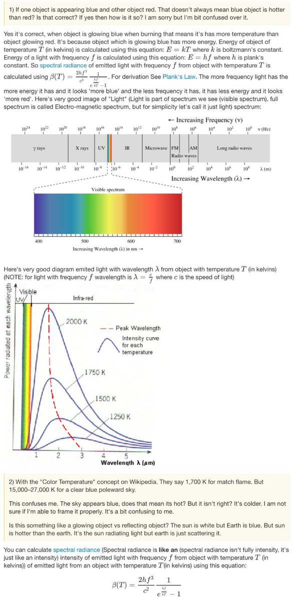
Of course i know this, and have written papers on spectroscopy, and posted such distinctions countless times on my blog, so it would really be appreciated if you would discontinue making false straw man statements about what I think or have not said, and then attacking me with those false straw men.
rgb once again makes a false analogy between ordinary Kirchhoff emission/absorption by CO2 at ~15um in our atmosphere [not amplified, stimulated, & coherent emission as in a light AMPLIFIED STIMULATED EMISSION of radiation LASER] . I’ve already explained several times on this thread why this is a completely irrelevant, false analogy and linked to the UC Davis Analytical Chem site which clearly explains why ““Unlike absorption, stimulated emission adds to the intensity of the incident light” in a CO2 laser:
http://chemwiki.ucdavis.edu/Analytical_Chemistry/Instrumental_Analysis/Lasers
The reason why a CO2 laser can melt steel is:
1. Stimulated emission increases intensity far beyond Kirchhoff absorption, which in our atmosphere = emission
2. The CO2 laser much shorter and much higher energy wavelengths of laser transitions in a CO2 laser are 9.6 & 10.6um as I showed in a diagram on this tread twice, irrelevant to the LWIR Earth bands centered around ~15um.
3. Stimulated emission from a laser makes use of a populations inversion of metastable states which many more electrons in the excited state than the ground state, which allows a very high intensity of coherent photons to be emitted.
4. Coherent waves from a laser are of much higher intensity since there is no destructive interference at the target
5. Not only is the beam very intense and coherent, it is also very thin, with little divergence, and very highly concentrated upon a small spot.
6. etc etc clearly demonstrating none of the above have any relevance whatsoever.
And nobody has been able to answer my question on how huge storms at the top of the Uranus atmosphere observed at 2800F are hot enough to melt steel. Presumably your answer is greenhouse gases, correct?
rgb says, “CO_2 radiates (in the 15 um band) when it is at 300 K. CO_2 radiates when it is at 250 K. CO_2 radiates at 200 K. It radiates at 400 K. The specific curve shapes that overlap the band will shift around, but it isn’t like it is forced to radiate at a temperature that one associates with its “peak” by some absurd alchemy involving \hbar \omega = k T. Again, learn to read the spectrographs you like to post. They actually do a peachy job of showing you what, in fact, CO_2 is doing as far as radiating energy away at the top of the atmosphere — radiating from a blackbody curve at 220K or 240 K or whatever, within the CO_2 absorptive window.”
Again you are making a false straw man argument of the opposite of what I’ve said, including here (to Phil):
The fact is no matter what the kinetic energy /temperature of CO2 is (assuming it is > 193K), the wavelength of the emission in the LWIR from CO2 will always be centered at ~15um, whether or not the kinetic energy/temperature of CO2 is 193K, 255K, 288K, 300K, 330K, 5000K etc.
The Planck’s/Wein’s laws equate BB frequency (v) and Temperature (T)
But even though CO2 is a mere molecular-line-emitter, not a true blackbody & much less than a true blackbody which has a Planck curve, bizarrely, Phil. somehow imagines CO2 is a magic super-blackbody with emissivity > 1, and which does not decline with temperature as observations have clearly shown.
In addition, in the OLR spectra I posted above you can see that at the ~15um CO2+H2O “hole”, the corresponding blackbody curve is that of a ~215-220K true BB, NOT a 280K, 288K, 300K, 330K blackbody, absolutely proving that I am correct and you Phil are absolutely incorrect.
http://lasp.colorado.edu/~bagenal/1010/graphics/earth_ir_emission.gif
rgb says “a photon has no temperature”
As I’ve said many times on this thread alone, the only thing a photon “knows” is its frequency/wavelength and Energy = hv. In turn, the peak temperature/energy of a true BB is determined by Planck’s Law for a particular frequency/wavelength/energy of a photon:
To assume CO2 can emit 15um photons than have higher energy than 15um photons from a true blackbody, and that those 15um photons can be thermalized by a blackbody at > 193K, breaks multiple laws of physics including 1st & 2nd LoT, Kirchhoff’s, Planck’s, Wein’s laws, Einstein’s photoelectric equation, photoelectric threshold wavelength, etc. [CO2 laser amplified stimulated coherent radiation absolutely does not occur naturally in the atmosphere and thus analogies to LASERs are false for the reasons above).
Then there is this:
http://www.phy.duke.edu/~rgb/Toft-CO2-PDO.jpg
“It is simply not factually correct to state that there is some sort of disagreement between the simple predictions of the Greenhouse model and observation over the last 165 years, unless and until you successfully impugn the data itself, e.g. HadCRUT4 in this figure. There are reasons to impugn the data, mind you, but taking the data at face value the fit to the log of the CO_2 concentration is impressive even without adding a single 67 year period sinusoidal with an amplitude of around 0.1 C.”
And:
“if you like, I get a TCS of around 1.8 C plus or minus maybe a whole degree. If the pause continues for another decade, it might pull the best fit down to 1.4 C per doubling, for example, and still produce a pretty good fit but with larger “natural” excursions due to physics and phenomena the model obviously does not include.
What it is not is evidence against the assertion that CO_2 increases warm the mean planetary temperature. Nor does it in any way justify the assertion that a 20 year pause means that the greenhouse effect itself is incorrect or nonexistent. It is silly to make these assertions — that just because temperature hasn’t gone up for 20 years, the GHE itself doesn’t exist and is “wrong”. What the GHE isn’t is alone. It isn’t the only thing going on. It may not even be the most important thing going on.”
http://wattsupwiththat.com/2015/05/12/22-very-inconvenient-climate-truths/#comment-1932077
http://wattsupwiththat.com/2015/05/12/22-very-inconvenient-climate-truths/#comment-1933114
That plot annoys me no end. With 5 parameters, you can make the elephant wiggle his trunk.
It is no more compelling than the top plot here, where the apparent agreement falls apart completely if you extend the plot out farther.
http://i1136.photobucket.com/albums/n488/Bartemis/extrapolation_zpsse2orlyc.jpg
How much more CO2 could possibly be released into the atmosphere given available technology to use it and the limited amount available? What will the atmospheric CO2 ppm be as a result?
Nobody really knows. The best value from my understanding is that atmospheric CO2 concentration will peak at 560 ppm plus or minus 10 ppm around the year 2100
I recently recounted all claimed supplies of coal, oil and natural gas and I got number around 1000ppm. But this only adds current 400ppm with 600ppm of all carbon reserves. So real number would be much smaller, I quite agree with bw’s 560ppm.
…. and the way logarithms work, this would give rise to another half-doubling of the effect of CO2 above the 280 ppm pre-industrial level. We are now at 400 ppm, the first half-doubling (of effect), and the empirically observed effects of this, using rigorous scientific principles are between zero and immeasurable for any global climate parameter.
I don’t, however, expect that there is any warmist out there who can multiply “zero to immeasurable” by two without some psychiatric problem manifesting itself.
Observed atmospheric CO2 ppm is a function of the kinetics of all CO2 sinks operating simultaneously with the releasing kinetics of all sources. Even in the most simplified equation setups, future predictions of pCO2 is a second order diff eq.
The implication of this is that “if emissions ceased tomorrow” ( a downstep change in total source kinetics), sink kinetics are higher and would lag due to biosphere greening of the higher CO2, longer growing seasons, and higher latitude biological growth (tree line advancement).
There is a flaw in the argument that the oceans take a long time to heat up and it is if surface temperatures are not rising we would not expect the ocean temperature to rise either. Is there a different Sun heating the oceans?
Another question. Then anthropogenic CO2 has been growing exponentially.
http://www.skepticalscience.com/images/co2_emissions.gif
Atmospheric CO2 however seem to have an unaltered linear growth rate.
http://www.optocleaner.com/CO2-NOAA.jpg
How can the claimed main source of CO2 be growing exponentially and not alter the slope of the atmospheric CO2?
The oceans have been warming. How much of the atmospheric CO2 is due to the warming oceans due to Henry;’s Law?
The big el ninos that we have had recently would be as a result of the surface temperatures rising and warming the ocean and not the el ninos warming the surface temperatures possibly.
this is a classic example of getting “balled up in one’s Underwear.” It begins with the simplifying assumption that all forcing comes from Greenhouse Gas CO2 that cannot change state at the Earth’s surface or in the atmosphere. “Dry Ice” results when CO2 changes state, and that occurs at MINUS 109 DEFREES and one atmosphere of pressure. This temperature/pressure combination does not occur naturally. The vast amount of energy absorbed or released when CO2 changes state to “Dry Ice” is used for convenient and effective refrigeration. Now, consider that CO2 remains a gas over the entire temperature range where Water has TWO naturally occurring state changes in the atmosphere – water to water vapor and water to Ice. Both of these state changes occur in normal atmospheric temperature and pressure ranges, and are acknowledged by meteorologists to be dominant forces in the Earth’s weather. Water Ice has temperature inertia, requiring vast quantum amounts of energy, to melt it. Liquid Water is the result of melting, and water itself can absorb vast amounts of energy as liquid water until it vaporizes, Water that vaporizes absorbs another vast quantum of energy when it changes state to water vapor. Water vapor releases that vast quantum energy when it condenses, liquid water releases its vast quantum energy when it freezes. Both of these state changes occur in naturally occurring temperature and pressure ranges constantly worldwide, CO2 only has its gaseous absorption and radiation capacity, and at its 0,4% concentration in the atmosphere, it cannot possibly drive water through its states, or even appreciably heat or cool the vastly larger concentration of water, water vapor and water ice in the dynamic weather atmosphere of earth, where humidity reaches 100%. So, taking state changes and liquid water and ice and even Water vapor out of the thermal energy exchange formulas is taking the vastly dominant components out. If you do that, then modeling atmospheric temperatures using just CO2 in its constant state is simple but so insignificant as to be meaningless. Weather modeling is based on understanding energy transfers, and it focuses on water, clouds, evaporation and freezing water ice. Yet, this Anthropogenic CO2 driven model takes no account of it and claims that the 10% of CO2 released by humans can control it all. The basic assumption that water in all its states. Changing states, dealing in astronomical numbers of energy can be left out of ANY Earth Climate model is absurd.
P u t I t. I n. T h e. M o d e l.
Another question, here is a chart of the earth’s radiance under clear and cloudy skys. Can clouds really lower the outgoing radiation by 88°K from 288°K to 200°K? Given that CO2 is basically constant, how can CO2 be blamed for the change when H2O has such an overwhelming impact?
http://www.mathstat.dal.ca/~folkins/Cloud-LWspectrum.jpg
co2islife “Can clouds really lower the outgoing radiation by 88°K from 288°K to 200°K?”
Point your remote-sensing infrared thermometer at the night sky. Where I live the temperature is below the bottom limit of -60 F. Point it at the underside of a cloud and even at night in the winter it measures about +20 F. The difference is enormous and the energy radiated down is obviously not going up.
“Given that CO2 is basically constant, how can CO2 be blamed for the change when H2O has such an overwhelming impact?”
The idea is expressed by the word “feedback”. A little extra heat evaporates a lot of extra water since the Earth is about 3/4 covered by water. Of course, many feedbacks exist, some amplifying the change and some working in opposition. Water is an enormously powerful transporter of heat from the equator to the poles; putting more of it into the atmosphere presumably permits more heat transport to the poles, causing them to warm faster than the tropics, which appears to approximately be the actual case. It would seem that an optimum probably exists.
Exactly. There is another chart that helps understand. It is in the first post at paullitely.com. Water is so much dominant, with a broad absorption spectrum. CO2 has a very narrow absorption spectrum
From your graph the upper curve is surface emission at about 280K with inter alia absorption by CO2 and O3 absorbing and higher in the atmosphere emitting (T ~220K & ~250K). The lower curve shows cloud tops emitting at ~200K with CO2 and O3 emissions from higher in the atmosphere (but warmer, ~220K).
Who first decided that H2O takes a back seat to CO2 in the radiative forcing arena? I’ve heard the argument that says because individual water vapor molecules, on average, don’t live as long in the atmosphere, that this makes water vapor IR absorption a feedback. To me, that’s not at all persuasive. It’s like saying that if the atmosphere contained zero CO2, it could not therefore, contain any water vapor. And that’s clearly wrong and stupid. So how about we bifurcate the two contributions, and weight the bigger one (water vapor) appropriately, and give it the respect it deserves, mathematically speaking?
Do the physics change the longer a molecule has been in the atmosphere? Can a photon differentiate between a CO2 molecule that has been in the atmosphere 1 day vs 5 years? Can a photon differentiate between a CO2 molecule created by man vs nature? Since when does “residency life” trump concentration? Also, no one seem to know what the “residency life” of CO2 is. I’ve seen estimates of 50 to 200 years in IPCC reports, and the best estimates I’ve seen put it about 5 years. Looking at the O2 chart CO2 varies on an annual basis by about 2%, so at most a CO2 molecule could be expected to reside in the atmosphere 50 years.
http://alanbetts.com/image/1/1200/0/uploads/co2data2-1278681362.jpg
Unless there is a reason CO2 made with C14 is removed at a higher rate than C12, it looks like the expected residency life is at most about 40 years, and no where near 50. Almost 100% of the atomic bomb created C14 created around 1963 is gone. 50% was gone in 7 years.
http://scienceblog.at/pics/2013/20131004/abb2.gif
Unless there is a reason CO2 made with C14 is removed at a higher rate than C12,
There is, C14 concentration in the atmosphere was doubled whereas that in the ocean was not, in the exchange process between atmosphere and ocean more C14 will enter the atmosphere than in the reverse. Also CO2 is transferred down into the deep ocean and is balanced by that due to upwelling from the deep ocean which is ~1,000 years old, any C14 coming back up will have undergone significant radioactive decay.
The effect of CO2 backscatter can be quantified OK, but I have issues with the means of deriving the climate sensitivity to the backscattered energy, which would seem to depend on assuming that the predicted sensitivity values are as defined. This would seem to be very like those equations we’ve all encountered which are reducible to 1=1.
Mike wrote: Rcy = 5.35 * ln(Cy/C0) – j * ((T0+Tcy-1)^4 – T0^4)
It seems to me that you should replace j with e*o, an “emissivity” times the S-B constant. Your value of j gives an emissivity of 0.204. When the earth is treated as a graybody with a surface temperature of 288 degK, emissivity is usually around 0.6. (In a comment above, I discussed why emissivity isn’t a very appropriate concept for an atmosphere. Ignoring that for the moment…)
When equilibrium has been reached and Rcy = 0 (increased outward flux from the warmer surface compensates for the forcing from CO2:
Tcy = 5.35*ln(2)/(4*e*o*T^3) = ECS
If e = 0.615, ECS is 1.11 (near the usual value for the no-feedbacks climate sensitivity). If e = 0.204, ECS is 3.3 degC – roughly the assumption that went into your calculation.
So far, you haven’t taken into account feedbacks – the change in OLR is not simply -5.35*ln(2) after a doubling of CO2.
” So now to calculate the change in temperature, we just need to know the climate sensitivity. Studies have given a possible range of values of 2-4.5°C warming for a doubling of CO2 (IPCC 2007). ”


I find this hard to accept based on IR measurements of sky and the Earth’s surface
This a clear sky day, about noon
This is concrete, grass, asphalt and sky.
Now the sky temp is through the atm window, but you can add Co2 forcing to this value.
Midnight clear day
Same concrete, grass, asphalt and sky.
So at least in the window this the temp the ground sees.
I finally got up before sunrise, now it was in the 90’s yesterday, and cloudy most of the night
Same concrete, grass, asphalt and sky, only this time your seeing cloud bottoms with maybe a small opening to clear sky, if it was clear, yet almost 70F warmer that is from water vapor, matching the tropical air yesterday vs the Canadian air for the other charts. You see this change in this temperature chart from my weather station
First observation, if you add what I think is the full Co2 forcing to low humidity sky, that’s about 180W / M2, water vapor adds a significant amount of forcing (I don’t have off the top of my head what another 40F to 70F forcing is), but clouds add significantly to even that. The forcing from Co2 alone has to be related to the LWIR emitted from the ground, and the surface and the temperature of that surface matters, alot, much more than the change in co2.
Any challenge to these comments about how these models are created?
1) They have a mis-specified model where an insignificant variable (CO2) is made significant, and the independent variable (temperature) is made the dependent variable.
2) They are clearly modeling a non-linear variable (temperature) with a linear variable (Over the time period studied)(CO2). That is why CO2 continued higher, the models continued higher, and the observations flat lined.
3) They have an underspecified model that is missing the most significant variables, ie solar, H2O, albedo, etc etc.
4) There is an extreme level of group think in the climate community, resulting in them all forming relatively similar and relatively wrong models. These charts represent a wild goose chase, a CO2 Witch Hunt, where the conclusion, CO2, was reached before the model was created, so they all made the same mistake. They focused on CO2. That represents a bias, not science.
5) Simply running a simple regression on CO2 and Temperature will expose the flaw in their theory. Running a “Stepwise” regression analysis will discover the true drivers of the climate, and I’m 100% certain CO2 won’t be one of the most significant variables in any model developed by an unbiased computer.
6) Given that a computer can prove the CO2 theory pure nonsense as I’ve described above, I would work to keep this “science” out of the courts if I were a warmist.
http://www.cfact.org/wp-content/uploads/2013/11/90-climate-temperature-models-v-observatons-628×353.jpg
7) They cherry picked an unusual and unrepresentative short time period when CO2 and Temperature did correlate relatively well to establish the relationships. They modeled a coincidence, not a causative correlation. Had they used the entire 600,000 year history of CO2 and Temperature data their models would have failed before they started. Not only did they model a coincidence, they created a model similar to lung-cancer causes smoking. They reversed the Y and Xs.
For once I agree with a part of one of your posts. Of course it is with Roy’s observation and graphic, not your other (still absurd, sorry) arguments. It isn’t a matter of consensus — it is a simple matter of fact that nearly all of the GCMs have predicted that the climate faster than it turned out to warm, some of the by almost one whole degree C. I also don’t disagree with the assertion that trying to fit only the last 165, or 200, or 300 years of temperature data to CO_2 is a particularly good test of the unprovable assertion that “natural variation over this interval does not matter”. There is actually no reason whatsoever to believe that this is true, and historically — outside of the infamous hockey stick itself — excellent reasons to think it false.
Sadly, we have no good way to know the temperatures we are fitting back into the remote past by means of proxies. I do not mean to say that we don’t have temperature estimates — only that they are almost never presented with error bars for a good reason. If they were, it would be too obvious that the error bars are close to 1 C (and tend to be smeared out over time as well, not really known month by month or year by year) and hence nearly all of the temperatures reported are so uncertain as to be nearly useless for the purpose of fitting or proving a model or verifying that natural variation is or is not important on century time scales.
Roy’s figure alone is a good and sufficient reason to rethink the climate models, and a very good reason not to use them to set very expensive global policy on the basis of their prediction of “catastrophe”. It does not mean that CO2 is universally beneficial, totally harmless in any concentration, cannot cause warming (because that is almost certainly not true and you won’t find a single competent physicist including Roy Spencer and Dick Lindzen — or myself, to the extent that maybe I’m competent — make any such assertion).
You might try learning from this instead of posting the very figures that prove to anyone who understands them that what you claim is incorrect.
rgb
Mike Jonas is to be congratulated in starting a stimulating discussion on certain aspects of current models.
I expect that subsequent posts will expose the logical nonsense ‘in the extreme’ which models are/have become.
Thankyou .
All evidence points otherwise. Nights over deserts show extreme variances from the daytime high temperatures. Areas with humid atmospheres show a very narrow range of diurnal temperature change. Antarctica shows extreme temperature variation from the wet coastal region to the dry inland region, and the temperature decay follows the loss of humidity. Bottom line, all climates have CO2 at 400ppm so CO2 can’t be the cause of the differences between humid and dry climates.
It looks like H2O can reduce the earth’s radiance by 288-200=88°K. CO2 is a constant, and doesn’t change. Only H2O can shift the IR spectrum, and vary the amount of heat trapped. CO2 can’t.
http://www.scielo.br/img/revistas/rbg/v21n1/a05fig03.gif
T = Tc + Tn. (Formula #1)
———–
To be clear temperature is not additive nor are the equivalents.
Heat in the atmosphere follows H2O, not CO2.
http://www.spectralcalc.com/atmosphere_browser/plots/guest547112018.png
http://www.spectralcalc.com/atmosphere_browser/plots/guest825527203.png
http://www.spectralcalc.com/atmosphere_browser/plots/guest122871090.png
I look forward to reading the series, as well as the “vigorous” debate that will no doubt accompany it.
My only comment so far is this. It is far easier to understand the GHE if one completely avoids looking at the Earth-Atmosphere-Ocean interface — the actual surface — and try to tally up things like back radiation, mostly because back radiation is mixed with conduction and convection and latent heat transfers and lateral heat transfers to the point where everything is both dubious and arguable. We cannot solve the coupled Navier-Stokes equations in our heads, nor can we solve them at adequate resolution from reasonably well known initial conditions with our best computers — manifestly, as co2islife’s reproduction of Roy Spencer’s figure above conclusively (IMO) demonstrates.
It is a lot easier to understand the GHE from spectrographs and from contemplation of the Earth as a system that is warmed at some rate by the sun through an atmosphere that is largely transparent to or reflective of direct sunlight (not terribly absorptive of, in other words). To remain at an approximate dynamical equilibrium temperature it has to radiate all of this power away so that ins equal outs, via radiation alone.
Some of the outgoing radiation comes directly from the surface and can be closely and reasonably associated with the blackbody curve for the temperature of the radiating surface. Some of that outgoing radiation is absorbed by the atmosphere, which is basically completely opaque at ground level to in-band LWIR in the absorption bands of greenhouse gas molecules. Note well — I do not reference back radiation, forward radiation, latent heat, what happens at the ocean’s surface to IR, whether or not convection is important — none of this matters. The surface does indeed lose energy to the near-surface atmosphere and pick energy up from the near-surface atmosphere in many, often complex ways, but the only thing that matters is that outgoing LWIR is almost instantly absorbed by the atmosphere in certain bands.
Way up at the top of the troposphere (at a variable, not terribly sharp height) the atmosphere becomes tenuous enough for radiation in the greenhouse gas bands to escape. Greenhouse gas molecules in thermal equilibrium with the general atmosphere at that height and above have around a 50% or better chance of radiating energy away from one of their in-band levels and having the photon make it out to “infinity”. Top of atmosphere spectrographs show that this energy is radiated away roughly consistently with a blackbody radiation curve in the absorption band of the relevant species at the temperature associated with that height.
Because of the (approximately adiabatic) lapse rate, the atmosphere at the height where transparency is achieved is usually much colder than the surface underneath.
The total radiation from any patch of the surface is thus (in very crude terms):
P = A * S + B * G
where A is the fraction of unblocked radiation, S is the power from the surface, B is the fraction of blocked radiation (at the surface) and G is the power coming from the greenhouse gases.
P must on average equal the incoming power from the sun for the earth to be in dynamic equilibrium. If it is smaller, the Earth accumulates energy from the difference and warms until S increases enough to rebalance the rates. If it is larger, the Earth loses energy from the difference and cools until the reduced S once again balances things.
Greenhouse gas concentrations and details in the quantum mechanics that dictate absorption make A, B and G all three somewhat variable on greenhouse gas concentration. The simplest way to understand the variation is that if one increases (say) CO_2 concentration, then the height where the atmosphere becomes sufficiently transparent for radiation in the CO_2 band to escape increases, as it depends on the mean free path of the in-band photons and whether or not they are likely to encounter another absorber molecule on the way out of the atmosphere. Increased height means colder from the lapse rate, which means that G goes down a hair. S has to go up a hair to compensate.
Note that this effect quite literally has nothing to do with what goes on near the surface. Surface energy can be transferred to the atmosphere by radiation, conduction, convection, latent heat, and by tiny pink unicorns that carry hot water bottles on their backs, as long as those unicorns don’t fly out of the atmosphere with the heat but allow it to escape via radiation. Increased concentration may or may not increase back radiation and this may or may not be interpreted as the “cause” of additional surface warming but it is a terrible way to tally it up because of the confounding stuff.
At the TOA it is simple. Detailed balance must be maintained, and to the extent that it is not the Earth warms or cools.
Note well that the Earth warms and cools much more than the CO_2-linked portion of this effect on a 1 to 5 year basis. IMO this means that it is never very far from true dynamical equilbrium, and I am deeply skeptical of any large amount of “uncommitted warming”. One gets a rather excellent fit to the data with a CO_2 driven warming model with no lag — temperature directly fit by a log of the concentration, with a warming per doubling of concentration of around 1.8 C. That doesn’t prove that there is no lag, but one does at the vary least have to show that a lagged, integrated model (that is of course much more complex) both fits the data and satisfies the fluctuation dissipation theorem when analyzing the laplace decomposition of the short time temperature fluctuations. I very much doubt that they are going to leave much room for a 100 year residual of any significant size.
rgb
“The simplest way to understand the variation is that if one increases (say) CO_2 concentration, then the height where the atmosphere becomes sufficiently transparent for radiation in the CO_2 band to escape increases, as it depends on the mean free path of the in-band photons and whether or not they are likely to encounter another absorber molecule on the way out of the atmosphere. Increased height means colder from the lapse rate, which means that G goes down a hair. S has to go up a hair to compensate.”
The geopotential height of the ERL is set by “triangulating” atmospheric center of mass, the fixed 255K equilibrium temperature with the Sun, and the tropospheric lapse rate, a function of gravity and Cp only. The ERL height is not affected by concentration of CO2 (other than a negligible effect of a tiny increase of Cp, which is *invesely* related to dT).
Again I have to disagree with you hockeyschtick. The top of the CO2 column, the level where radiation to space can occur, is in the lower stratosphere. The stratosphere exhibits temperature inversion ie: it gets hotter as you go up. By the time one gets to near the top of the stratosphere the temperature is back to about 280K so if the emission altitude rose it would reduce the warming effect. Alas of course things are not quite so simple.
However there is a MUCH (and I do mean MUCH) simpler way to prove CAGW false. The whole thesis of CAGW is that rising CO2 acts as a blanket reducing Earth’s energy loss to space so that with constant energy input there is an imbalance causing Earth to warm. Energy loss to space is measured as outgoing long wave radiation or OLR and this has indeed been measured since the late 1970’s. Thus for CAGW to be correct CAGW should have been falling during this time but unfortunately it has been rising. Opps!!!! Of course one could argue that OLR would rise as Earth’s temperature rises but then the rise in OLR would be the rise due to Earth’s warming minus the fall due to increasing CO2 ie: the rise would be very significantly less than predicted by warming alone. Ahh but unfortunately the rise in OLR is GREATER than would be predicted by the temperature rise alone. That means Earth is finding it easier to lose energy to space not more difficult and as far as I am concerned that falsifies CAGW beyond redemption.
Michael Hammer says, “However there is a MUCH (and I do mean MUCH) simpler way to prove CAGW false. The whole thesis of CAGW is that rising CO2 acts as a blanket reducing Earth’s energy loss to space so that with constant energy input there is an imbalance causing Earth to warm. Energy loss to space is measured as outgoing long wave radiation or OLR and this has indeed been measured since the late 1970’s. Thus for CAGW to be correct CAGW should have been falling during this time but unfortunately it has been rising. Opps!!!!”
Agreed, Dr. Nor van Andel’s posts on by blog have been pointing that out for years
http://3.bp.blogspot.com/_nOY5jaKJXHM/TI-1aWFUoFI/AAAAAAAABRs/tf6HawUmjC0/s400/Fullscreen+capture+9142010+104234+AM.jpg
http://hockeyschtick.blogspot.com/2014/10/analysis-shows-missing-heat-has-gone-to.html
“Again I have to disagree with you hockeyschtick. The top of the CO2 column, the level where radiation to space can occur, is in the lower stratosphere. The stratosphere exhibits temperature inversion ie: it gets hotter as you go up.”
No, radiation emission/absorption from CO2 occurs at all levels of the atmosphere from 0-80km+
For P < 0.1 atm, CO2 preferentially transfers energy via collision with the remaining 99.9% of the troposphere, which increases convective cooling. Nonetheless, CO2 does also absorb and emit ~15um/193K LWIR photons from 0-80+km, cooling the stratosphere, mesosphere, thermosphere.
What the warmists themselves cannot agree upon is how to explain why those 193K CO2 photos allegedly warm the much warmer troposphere, while simultaneously cooling just as warm or warmer stratosphere. No coherent answer to this exists, since it is unphysical.
The ERL is not in the stratosphere, it is in the mid-troposphere exactly at the center of mass of the atmosphere ~5.5km geopotential height.
“The ERL height is not affected by concentration of CO2”
wrong.
Typo above: “For P > 0.1 atm, CO2 preferentially transfers energy via collision with the remaining 99.9% of the troposphere, which increases convective cooling….”
” Increased height means colder from the lapse rate, which means that G goes down a hair. S has to go up a hair to compensate.”
Only if you hold the lapse rate, and temperature at ERL, constant. TOA is not so simple, after all.
“One gets a rather excellent fit to the data with a CO_2 driven warming model with no lag — temperature directly fit by a log of the concentration, with a warming per doubling of concentration of around 1.8 C. “
It’s a meaningless fit using 5 parameters. You could fit Von Neumann’s elephant with that.
Temperature of the ERL is fixed at the equilibrium temperature with the Sun = 255K
Height of the ERL is also fixed at the center of mass of the atmosphere at ~5.5km geopotential altitude.
Thus, both T and h of the ERL are essentially constants which are not a function of GHG radiative forcing
You are referring to the wrong curve. I’m talking about the two parameter fit to no-feedback, CO_2 only warming, precisely the model this article is examining. If you take the forcing model to be (as given above and many places elsewhere)
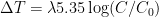

 in this is basically irrelevant — it is just matching up the two curves, and the zero of the anomaly is after all arbitrary — this fit has for all practical purposes one degree of freedom (but call it two if you like, as long as you recognize that one of them is just moving the whole curve up and down to get the best match). That is, I get
  .
. (or better yet, forget
  and shoot directly for the 2.62 as being all that matters even if the 5.35 itself is not precisely known as well).
 will end up larger when “uncommitted warming” resolves, although I am very skeptical about our knowledge of or ability to resolve long time scale relaxation and see little need provided by some failure of the fit itself to include a lag (and one would have to show that the convolution of the formula above with a lagged kernel would still lead to a log fit, not at all clear). And there is a very definite probability that it is smaller than 0.5, given the probability that HadCRUT4 has been at least somewhat inflated by selective “adjustments” that are at least unlikely (in the strict sense of the term) to have been as monotonic and systematic as they have turned out to be.
 than acknowledged by the modelled studies above.
then, to be precise, the fit is:
Since the
This is just under the low end of the estimate discussed in the top article, and is the result of directly fitting the algebraically predicted functional form to the unlagged data. It produces an excellent fit to the data trend. The sinusoid is — as you know perfectly well if you actually read what I say any time I post this figure — an amusement, not something to take seriously. It has been pointed out, correctly, that the temperature has an apparent periodic cycle superimposed on top of a general warming. I just for grins fitted this to show that this is true, that the fit improves (maximally) if you assume an amplitude of around 0.1 C and a period of 67 years. That isn’t suggesting that this variation is predictive in any way — I do not do so as I have no idea why it is there (and neither, frankly, does anybody else, although some will claim that they do). It could be, and perhaps even probably is, purely spurious, the result of a transient chaotic cycle. Some fraction of the overall warming could be this as well. I’m not addressing that.
What I do say is that it is not the case that the simple, basic model of CO_2 driven warming fails to describe the HadCRUT4 reported temperature anomaly from 1850 to the present. It does not. It fits the data remarkably well, although with a much lower climate sensitivity than the GCMs or the IPCC would have you believe. It provides little incentive to go much further and search for complex volcanic or anthropogenic aerosol or PDO/ENSO linked effects. It actually works as a single relevant parameter predictor of the entire climate series within 0.1 C or so, and is not fitting a random function I just made up, it is fitting the function one expects to find from the physics.
This means that if you want to assert that CO_2 does not cause any (significant) global warming, the onus of proof is very much on you to prove that it does not, given that a very sound physical theory predicts it and the prediction is in very good agreement with 165 years of observations. Even if the observations themselves have been tweaked — and I freely recognize that possibility, as well as show the error bars HadCRUT4 acknowledges in the fit curve and criticize them as being obviously too small for most of the past and inconsistent with things like the difference between HadCRUT4 and GISS in the present — it seems to me at least pretty likely that the empirical connection between CO_2 and warming is far from refuted by this agreement and that most reasonable people would agree that it is in fact supported by the last 165 years worth of data, with what are probably fairly substantial error bars on
It could be that there is indeed a lag and that
But please, Bart, do not attribute to me things that I have not stated or asserted. I clearly explained this almost every time I’ve posted this curve — the sinusoid is for grins, not because it should be taken seriously at least until there is a creditable explanation for it. The thing that is not for grins is not fitting an elephant. Not at all. It is rather proof of the simple fact that a log dependence on CO_2 concentration fits the last 165 years of (possibly adjusted) data remarkably well, if with a smaller
I like direct fits over GCMs, personally. The GCMs fail in multiple ways, and have countless assumptions. The fit above has one — Carbon Dioxide concentration is logarithmically related to the dynamic equilibrium temperature of the Earth’s climate. Turns out this assumption is pretty good.
rgb
It is also all too convenient that a starting point for temperature series is AFTER the Dalton Minimum, in the long more linear recovery period.
” It fits the data remarkably well, although with a much lower climate ”
I “worry” that the reason they fit so well is that a log function is baked into the temperature series itself, because one can argue I don’t know what I’m doing with the temp data I’m using, but those measurements don’t have the same rising curve.
Nine physical reasons why increased CO2 does not increase the ERL height or decrease the fixed temperature of the ERL = 255K = equilibrium temperature with the Sun:
http://hockeyschtick.blogspot.com/2014/11/why-global-warming-is-not-explained-by.html
Dr. Brown, please kindly have a look at Kimoto’s published paper e.g p 1061 finding why the no-feedback Planck response is exaggerated due to the false assumption of constant effective emissivity of the atmosphere.
http://hockeyschtick.blogspot.com/2015/07/collapse-of-agw-theory-of-ipcc-most.html
other questions for Dr. Brown, if I may:
1. The line-emission bands of CO2 in the LWIR is centered at ~15um, regardless of concentration, correct? (& even if the bands are slightly widened by increase concentration, the center of the bands remains ~15um, correct?)
2. If CO2 was a true blackbody (even though it is a mere-line emitter), what is the peak/maximum emitting temperature of a blackbody with peak emission at ~15um?
3. Can radiation from a true blackbody with peak emission at 15um be thermalized and transfer heat energy to a true blackbody with a peak emission at 5um?
I’m not certain what your thrust is here. Look directly at the outgoing spectra. I don’t care what causes the bites in the CO_2, water, and ozone bands. It could be invisible fairies or pink unicorns, or it could be precisely what it appears to be — radiation from greenhouse gases in the upper troposphere where the temperature is correspondingly reduced by the lapse rate. There are many of these spectrographs out there — I have Grant Petty’s book sitting about three feet away from me and he presents several in it taken looking down at very different kinds of terrain at different latitudes — and in each case this is a very sensible, quantitative interpretation of the spectra.
Ultimately, all that matters is that a) ins have to equal outs for the Earth to be in equilibrium, as opposed to warming or cooling if ins exceed outs or vice versa; b) there being some functional variation of the transparency of the atmosphere in the greenhouse bands with concentration.
Again, the latter isn’t really open to “discussion”, because water vapor varies tremendously and we have plenty of spectra showing what happens to radiation as it does. If you make the atmosphere substantially more opaque by increasing water vapor content, you drop the emission temperature in the water absorption band. Are you going to try to assert that if we increase CO_2 we aren’t going to drop the emission temperature in the CO_2 absorption band by driving its emitted radiation level up? Or are you going to assert that the lapse rate will increase at exactly the same rate to compensate (as Bart and several others seem to want to imply without substantiating how, or why, this would happen just for CO_2 where it does not happen for water).
Water is, of course, more complicated than CO_2 — this isn’t intended to say that water feedback is strong and positive as my own fits to the data suggest nothing of the sort and perhaps imply the opposite (depending on how much you believe “the models”). But in my opinion — take it for what it is worth — it is extremely unreasonable to expect the average all conditions lapse rate to exactly compensate for increased CO_2, if it compensates at all. If a temperature-driven increase in lapse alone compensated for temperature increases, it would be very difficult to explain a warming climate ever, and outside of that, why would it pick on CO_2? The atmosphere radiates (thermally) from a bunch of molecules, sometimes at different ERL. OTOH, it is very reasonable to expect ERL from CO_2 (again, however the energy being radiated gets there) to increase with CO_2 concentration simply because the mean free path is a simple function of concentration. Double the concentration, you reduce the MFP by 2^-1/3 = 0.8, you have to go up further in the exponentially decreasing atmospheric density to reach a MFP that can reach infinity for upward directed in-band photons, and it will almos certainly be colder up there unless “a miracle happens”.
So sure (to reply to Bart as well) — I could be wrong, the model could be wrong, the papers that compute the expected warming from CO_2 in line by line computations could be wrong, evvybody could be wrong, but — damn, the basic model that results from the line by line computations and simple averages fits the data doesn’t it…
Could it fit back to 1000 CE, or 10,000 BCE? I doubt it. But at some point there is some slowly varying climate stuff involving orbital cycles that at the very least slowly shifts the all-things equal equilibrium, and there may well be natural stuff with substantial amplitude and periods or time constants order of centuries as well. The climate is not a stationary process even without varying CO_2. You don’t have to point it out, I know it perfectly well. So we have some unknown amount of natural variation mixed in with any CO_2 driven effect. Maybe half the warming was natural, and only half was due to CO_2 increases. Maybe total feedback is strongly negative. Even so, I personally would be very, very surprised if the partial derivative of “average equilibrium temperature” (if one could ever reasonably define such a thing) with CO_2 concentration was, averaged over all confounding variables in the neighborhood of the present, not positive.
And even if some of the recent warming is natural, that doesn’t alter the simple empirical fact that it is damn well fit by a log of CO_2 concentration with a sensitivity very close to the theoretical no-feedback estimate.
rgb
To be a bit more precise in my response below (and to appeal to outside authority of what surely is obvious anyway):
http://www.aos.wisc.edu/~aos121br/radn/radn/tsld015.htm
to quote:
So none of the assertions you make are correct. It isn’t fixed at some temperature. It isn’t fixed at some height. It isn’t the same for all wavelengths. It isn’t constant in time. It isn’t constant with respect to variation of greenhouse gas concentrations. It is not constant.
All of which you would know if you bothered to look at a single TOA spectrograph. Look, co2islife posted one above (although he doesn’t seem to understand how serious an argument it is against his desired conclusions). Go take a peek at it. By a copy of Petty’s book. Peek at a few more. Look up some papers with still more. It isn’t that hard to understand.
rgb
rgb says “you would know if you bothered to look at a single TOA spectrograph. ”
Please be nice, I’ve been looking at them for several years and have a degree in physical chemistry. In my reply below I posted an image of a TOA spectrograph that I put annotations on more than one year ago, explaining why the ~15um “hole” in the center “corresponds” to a true blackbody with a maximum peak emission temperature of ~215-220K. Even though GHG line-emitters are not true BBs, assuming they are, a BB emitting photons at ~15um/215-200K cannot be thermalized by a warmer BB in which all of those lower-E microstates are already saturated.
“It produces an excellent fit to the data trend.”
It’s not an impressive fit. It doesn’t match any of the variations. It just sort of hugs the middle. Well, the hugging the middle is low information. You could make a fit with just about any low order polynomial.
It’s not anything like being able to fit everything, across the entire frequency spread, as the temperature anomaly fits the rate of change of CO2.
“…given that a very sound physical theory predicts it…”
No, it does not. It is just one possible outcome of one influence. It’s like saying that there is a very sound physical theory which predicts that, since gravity pulls one object towards another, the objects will eventually collide.
However, that completely ignores the role of energy and angular momentum in maintaining an orbit. Just so, other influences which have been ignored can prevent the seemingly ineluctable conclusion that has been drawn on the effect of increasing CO2 in the atmosphere.
rgbatduke writes “At the TOA it is simple. Detailed balance must be maintained, and to the extent that it is not the Earth warms or cools.”
It would be more accurate to say the Earth accumulates energy rather than “warms” or “cools” because it is feasible that atmospheric processes could warm or cool above the surface. The physical requirement to retain equilibrium is that the ERL temperature change. This could happen through a change to the lapse rate for example.
“The physical requirement to retain equilibrium is that the ERL temperature change. This could happen through a change to the lapse rate for example.”
Yes exactly, well illustrated in Kimoto’s new paper Fig 2 (and the unphysical fixed lapse rate assumption of the IPCC et al shown in Fig 1 for comparison).
rgbatduke:
You conclude saying
Me too, especially when the so-called committed warming which is ‘projected’ to now exist has vanished as I explain in my above post.
Richard
Yeah, there are a lot of reasons to doubt this, aren’t there, the ability of the “pause” to override a supposed long term imbalance among them. At the very least one needs a pretty sophisticated new theory to explain Trenberth’s missing heat problem with oceanic uptake and perhaps a bit of black magic.

 , and might well be compensated for in the bias build into HadCRUT4 and GISS, neither of which are (IMO) particularly trustworthy given the pattern of “adjustments” and how they correlate with CO_2 concentration.
OTOH, I don’t know what to make of the CERES data that seems to show an average 0.5 W/m^2 or so imbalance in the first place. That’s such a small number it seems as though ANY sort of systematic error in the apparatus would be enough to make it pure noise, and I don’t quite see how they could calibrate the apparatus to that degree of precision — they are basically integrating over all wavelengths both the incoming and the outgoing radiative flux over the entire surface, and since this fluctuates substantially and involves integrating over all angles, even a small systematic error looks like it would be plenty to make this meaningless. Yet there is is, and I don’t have any good reason to consider it anything but a good faith result. If valid, then the Earth is indeed lagging by a hair.
How much of a hair? Well, a back of the envelope estimate of the hair seems as though it would be:
Or (assuming my arithmetic does not suck, always a bit question) a bit less than 0.1 C. That is if we have a radiative imbalance of 0.5 W/m^2, and the Earth is at 288 C, Stefan-Boltzmann suggests that it would only have to warm by another 0.1 C to be in balance. So maybe the fact that SB has to be adjusted for the GHE makes it 0.2 C. That’s chump change in
So I’d believe in up to 0.2 C of “uncommitted warming”, but find it very difficult to justify any larger number in either data lag or SB plus CERES data, and suspect that the baseline 0.08-0.09 C is a better estimate. Indeed, since a lot of the heat is coming out at the equator where it is much warmer than the 288 average, even this might be an overestimate. If 1/3 of the surface area is over 300 K on average (probably fair enough) the 0.08 C estimate is probably fairer. This is about a 5 to 10 year lag of “uncommitted warming”, and since I eyeball an autocorrelation time in HadCRUT4 (allowing for non-stationary data) of around 5 years, that is far from crazy. By one decade, two full cycles of warming and cooling in natural fluctuations have typically occurred, and a year like this one with a big El Nino (finally!) will probably make outgoing radiation exceed the temperature for a year or two as it dumps heat into the upper troposphere and stratosphere where it can radiate away comparatively rapidly.
rgb
“That is if we have a radiative imbalance of 0.5 W/m^2, and the Earth is at 288 C, Stefan-Boltzmann suggests that it would only have to warm by another 0.1 C to be in balance. ”
Assumes:
1. Stefan-Boltzmann law is applicable to GHG line-emitters, which are not true blackbodies and for which emissivity decreases with T
2. Assumes effective emissivity of atmosphere is a constant; εeff is not a constant but a complicated function of Ts and the internal variables Ij as shown in Kimoto 2009, thus exaggerating the Planck feedback parameter
3. Assumes non-radiative heat transfer from convection/evapo-transpiration, which dominate ~92% of tropospheric heat transfer, cannot easily overcome & extinguish a small radiative imbalance.
That’s why we call them “back of envelope calculations” and why I offer up that it could easily be off by a factor of two or even more either way.
You keep bringing up SB vs GHG’s, which is all lovely but instead of pointing out that emission from them is “complicated” — line by line computations are indeed complicated, and there are line by line computations out there that give results in at least rough agreement with the simple log model, which is why people still pay attention to the simple log model — why not just look at the spectra and see what they say?
They say that emission from the GHGs is in fact much lower in intensity in their emission bands than blackbody radiation directly from the surface would be. And that’s all that the greenhouse effect depends on!
Note well that it doesn’t make a damn bit of difference how the heat is transferred from the surface up to the top of the atmosphere. All that matters is how bright the outoing radiation given off by the atmosphere itself is up at the top of the atmosphere, because this is the only way the heat/internal energy can actually leave the system from the atmosphere at all, keeping the top cool, permitting convection, and driving the ALR in the first place. And to the extent that integrated power doesn’t leave the earth system at the top via atmospheric radiation, one way or another the system will have to warm until the surface brightness (and further adjustments to the atmospheric brightness) compensates.
That’s why I don’t like all of the bizarre pictures people make up of radiation and latent heat going up and going down as forward or backward radiation, or convection, or whatever. WHO CARES? To understand the GHE it suffices to know ONLY that the atmosphere is lapsed and opaque to radiation from the atmosphere itself until the density of each GHG species is reduced to where photons it emits upward are no longer reabsorbed before they escape. That’s it, end of story. All incoming radiation has to be lost in equilibrium by outgoing radiation. If the intensity of radiation from the GHGs is greatly reduced compared to the ground, you have a GHE. Spectroscopy strongly suggests that one can radiate from different heights from different GHG species as each one can have its own ERL (where the absorption bands don’t overlap).
I also don’t understand why you keep asserting that the ERL is “fixed” by this or that. The ERL isn’t even a sharp height. It varies day to day for water vapor in particular, because water vapor concentration is highly variable through the troposphere. It also varies with things like pressure (and by implication, local density) day to day, hour to hour. It is different for water vapor and for CO_2 (the latter being nearly constant except where it has band overlap with other GHGs, where water vapor itself varies even where it DOES have overlap with other GHGs). It is completely unreasonable to assert that ERL won’t vary at all with CO_2 concentration as the distance between CO2 molecules reduces (with a doubling) by a factor of 0.8. Why bother even trying to understand why CO_2 is opaque, mean free path and so on, if you’re going to make that big a mistake and just say it doesn’t matter right where it matters the most?
rgb
rgb says, “You keep bringing up SB vs GHG’s, which is all lovely but instead of pointing out that emission from them is “complicated” — line by line computations are indeed complicated, and there are line by line computations out there that give results in at least rough agreement with the simple log model, which is why people still pay attention to the simple log model — why not just look at the spectra and see what they say?”
Please have a look at this new paper, which uses 2 state-of-the-art line-by-line radiative codes (including that used by IPCC models) and states countless times that at the current Ts=288K, GHG LWIR is causing *cooling* of the surface:
http://hockeyschtick.blogspot.com/2015/07/new-paper-finds-greenhouse-gases.html
In addition, Manabe’s models and subsequent models Hansen et al show CO2 photons, limited to a peak BB emitting temperature of 193K & corresponding to a peak BB wavelength of ~15um falsely emitting radiation at up to 330K/8.8um. This is physically impossible for molecular line-emitter CO2 which only emits ~15um in the LWIR.
Regarding the ERL height/T it is of course a theoretical concept, and of course emission of LWIR occurs at all levels of the atmosphere. However, the Earth temperature seen from space is 255K, which also is exactly the same as the T of a BB at Earth’s distance from the Sun = 255K.
Countless references, including one I already linked to, say Te=Terl=T(seen from space)=255K. Do you not agree with this?
What does this even mean? Are you trying to assert that all the radiation is coming from a layer 5+ km up at a temperature of 255K? Or are you just stating the obvious, the energy has to be (approximately) conserved? for some processes at some point in the past. It isn’t that hard for a simple model like this.
So no, I do not agree with this. There are many ways of defining the average temperature of the Earth. One of them is the fourth root mean fourth power averaged over the surface. Another is the simple average over the surface. Neither of them will precisely correspond to transforming the average outgoing radiation into a temperature, because the Earth doesn’t radiate from a single surface at a single temperature in a perfect blackbody curve. It arguably radiates from a piecewise continuous set of blackbody curves associated with both the mostly transparent band(s) and the completely absorbed bands. And those bands can at least reasonably be associated with the temperature of their ERL, which might be different from other parts even of the bands of the same molecule and are likely to be different for different molecules with different concentrations.
I have to say that I was amused by the continuing effort (in some of the linked papers on your site) to make all of the warming of the Earth due to the ALR — “gravity done it” — without ever worrying about how the atmosphere cools at the top. Cools as in actually loses energy. Words fail me. Talk about violating the first law…
Well, no they don’t, but I’m tired and this is an old discussion that was silly the first three or four times I engaged in it. The ALR is without any doubt an important component of the GHE. But so is the cooling of the atmosphere from the top with IR-coupled gases that the atmosphere in general is opaque to.
The other papers you linked appear to be making claims that — to me at least — are either directly contradicted by reality or simply compute the warming produced by the greenhouse effect differently distributed but still net warming. Greenhouse gases are net cooling at the poles and net strong feedback warming at the equator? Because that appears to be the breakpoint of the temperatures given, doesn’t it? So either the papers predict more warming than cooling (and hence agree with the global average temperature data from 1850 to the present, that there is a net positive global warming due to the GHE (concentrated at the tropics, in spite of cooling at the poles) that seems inconsistent with the distribution of the observational data in the NH, at least, or else they predict global cooling through 400 ppm in which case they are directly contradicted by the data. Either way, I got no beef with them — I don’t try to predict how or where the upper atmosphere loses energy, only that ERL is modulated by concentration in band in any given greenhouse gas species and that depressing emissions in any band has to increase them everywhere else, including the surface, to remain in detailed balance.
Again, it isn’t that complicated. There is no doubt that atmospheric mass and density and the lapse rate are relevant to the overall GHE, but it is also simply not true that there is a single “ERL”. The atmosphere cools from a thick slab of heights, via radiation from greenhouse gases and not because of “gravity” (which is a conservative force after all). Greenhouse gases are one of the major factors that establish the tropopause, because you cannot sustain convection without cooling the top of the gas column. They call it adiabatic cooling for a reason!
But I should probably grade papers instead of walk through all of this — again — instead of commenting on all of the other things on your site that are just plain wrong, such as the assertion that any aspect of the GHE violates the second law and so on. They just make me tired-er. If you have a degree in physical chemistry you should know better. Seriously.
One last time. Buy a copy of Grant Petty’s book, simply to give yourself a fair shot at understanding this stuff, don’t just look for somebody that says something you want to agree with and that sounds like they are saying physics-y stuff. Look at the single layer model that he lays out in chapter 6. We can all argue about whether or not this model is a fair representation of the dynamics of the real atmosphere. I don’t think so, and I don’t think Petty thinks so. It is a single layer model and the real climate system is much more complex. But it is bone simple to walk through this physically valid model and observe that the laws of physics are satisfied by the elements in the model, and that the model is the first law of thermodynamics turned into a differential equation and used to find the stationary state, and that the heat transfers in the model do not, I repeat not, violate the second law of thermodynamics. Again, you must have had to compute
That should eliminate, once and for all, the notion that anything about the greenhouse effect per se violates first or second laws, that cold can’t heat hot and all that bullshit (none of which is relevant to the problem or a description of what is going on). Gravity can’t heat anything that isn’t collapsing, for that matter, because it is a conservative force and does no net work on any atmosphere with a density profile that is, on average, constant — and we do love the first law of thermodynamics, with its term involving external work. But surely you know that, right?
rgb
After a bit of reflection (and a trip to the CERES website to look) it doesn’t look like CERES instrumentation is capable of resolving 2 W/m^2 imbalances either way, let alone 0.5 W/m^2. I’m not certain where I read that it did — maybe in one of WIllis’ posts? He’s looked at the CERES data (I found it difficult to even see HOW to find and download usable CERES data, I hate the way they distribute this stuff, with link after link instead of just putting up a downloads directory with an index and some READMEs). But the one page I did find going through the CERES site more or less stated that CERES instrumentation has an unknown bias and is not suitable for computing net radiative imbalance at the TOA. In which case I have no idea where any such numbers come from. They are certainly bandied about often enough; I’ve probably been too uncritical.
rgb
” it doesn’t look like CERES instrumentation is capable of resolving 2 W/m^2 imbalances either way, let alone 0.5 W/m^2. ”
What I’ve read is that they are precise, but not accurate, so they do what they do everywhere else, they decide based on their model it should be about 0.5W/m^2, and then just adjust the measurements.
hockeyschtick July 26, 2015 at 4:12 pm
In addition, Manabe’s models and subsequent models Hansen et al show CO2 photons, limited to a peak BB emitting temperature of 193K & corresponding to a peak BB wavelength of ~15um falsely emitting radiation at up to 330K/8.8um. This is physically impossible for molecular line-emitter CO2 which only emits ~15um in the LWIR.
Yet again your mistakes, there is no ‘peak BB emitting temperature corresponding to a peak BB wavelength of ~15um’ . Black bodies of any temperature will emit at 15 micron.
Black Bodies are broadband emitters of EM, so of course they emit at 15u for a wide range of temperatures, but at 193K, the peak wavelength is 15u, do you agree with that?
If you had a vacuum dewar with a single Co2 molecule chilled to ~0K, what would happen if you fired a single 14u, a single 15u, and then a single 16u photon at it in 3 unique test? And what would the temperature be of the molecule be after the photon was sent if it was captured but not emitted?
Here’s the spectral radiance for a BB emitting at 15micron:
190K, 1.01
193K, 1.10
250K, 3.46
290K, 5.96
300K, 6.68
330K, 9.07
The last time this topic (photon temp) came up I pointed out this link on Co2 Lasers.
http://www.laserk.com/newsletters/whiteCO.html
Lasers are line emitters, and in the case of this Co2 laser (@10u), they do comment on photon temperate.
Now full disclosure, I have 10u temp as about 289K (62F), 5 times room temp would be ~7.5u some ~450K (~350F), it’s possible when the photon temp was calculated he mixed the two up, as the 10u 289K is numerically close to 7u’s 285F.
To further go along with this though he says this (the next sentence after the line quoted above).
350F should not need cryogenically cooled photoconductors, where they might be useful if the temp from the laser being measured was 62F.
micro6500 July 27, 2015 at 8:12 am
“Yet again your mistakes, there is no ‘peak BB emitting temperature corresponding to a peak BB wavelength of ~15um’ . Black bodies of any temperature will emit at 15 micron.”
Black Bodies are broadband emitters of EM, so of course they emit at 15u for a wide range of temperatures, but at 193K, the peak wavelength is 15u, do you agree with that?
Yes I have no problem with that but hockeyschtick is asserting that CO2 (or a black body) is incapable of emitting at temperature in excess of 193K. A misinterpretation of Wien’s law, claiming that 193K is the maximum temperature at which a 15 micron photon can be emitted!
“Climate scientists/modelers ever since Manabe et al have falsely assumed CO2 can radiate at emitting temperatures >193K and their papers show CO2 falsely emitting at temps up to 330K. This is physically impossible.
Frankly total BS!
micro6500 July 27, 2015 at 8:59 am
The last time this topic (photon temp) came up I pointed out this link on Co2 Lasers.
“Many applications have been suggested for CO2 lasers, but only a few of these have been given serious consideration and analysis. This is partly because little engineering has been done at 10 microns. Photon energy of about 0.1 eV is only about five times room temperature.”
http://www.laserk.com/newsletters/whiteCO.html
Lasers are line emitters, and in the case of this Co2 laser (@10u), they do comment on photon temperate.
Yes and CO2 lasers at 10.6 micron are used to melt steel!
According to the ‘schtick’ its photons correspond to 273K and shouldn’t be able to heat steel at 300K!
According to him he has a degree in Physical Chemistry, he must have slept through the lectures on spectroscopy.
Might I suggest this is a misunderstanding, I think, he’s saying the Photon can not be more than 193K, not that the Co2 Molecule can’t be over 193K, or that it can’t be over 193K and still emit a 193k (15u) photon.
Again I’ll plead misunderstanding, that Co2 laser emitting 10u cold photons, can emit a lot of them, and if they are thermalized in steel in a small enough area they will melt steel. But if they are not thermalized, I don’t think it will do any warming. In the case of steel it’s the flux rate not that wavelength that transferring enough energy to melt steel.
micro6500 July 27, 2015 at 9:57 am
“but hockeyschtick is asserting that CO2 (or a black body) is incapable of emitting at temperature in excess of 193K.”
Might I suggest this is a misunderstanding, I think, he’s saying the Photon can not be more than 193K, not that the Co2 Molecule can’t be over 193K, or that it can’t be over 193K and still emit a 193k (15u) photon.
Yes it’s a misunderstanding by him. For a start a photon doesn’t have a temperature, secondly he says:
“Climate scientists/modelers ever since Manabe et al have falsely assumed CO2 can radiate at emitting temperatures >193K and their papers show CO2 falsely emitting at temps up to 330K. This is physically impossible.
There’s no room for ambiguity in what he says and it’s flat out wrong!
“Yes and CO2 lasers at 10.6 micron are used to melt steel!
According to the ‘schtick’ its photons correspond to 273K and shouldn’t be able to heat steel at 300K!”
Again I’ll plead misunderstanding, that Co2 laser emitting 10u cold photons, can emit a lot of them, and if they are thermalized in steel in a small enough area they will melt steel. But if they are not thermalized, I don’t think it will do any warming. In the case of steel it’s the flux rate not that wavelength that transferring enough energy to melt steel.
According to ‘the schtick’s’ crazy theory a 10 micron photon represents a temperature of 273K and can’t thermalize a warmer body, like a 300K piece of steel. What one can’t do neither can a million etc., but yet I can focus a 10.6 micron laser bean and cut through steel with it. Of course it’s the flux rate that’s important not the wavelength, but that’s not what ‘the schtick’ says, he says it’s all about the wavelength.
rgb re HS: “Countless references, including one I already linked to, say Te=Terl=T(seen from space)=255K. Do you not agree with this?”
rgb: “What does this even mean? Are you trying to assert that all the radiation is coming from a layer 5+ km up at a temperature of 255K? Or are you just stating the obvious, the energy has to be (approximately) conserved?
So no, I do not agree with this.”
I do mean Ein = Eout, conservation of Energy, and I absolutely don’t mean ” all the radiation is coming from a layer 5+ km up at a temperature of 255K.” Radiation is absorbed/emitted at every single level 0-100km in the atmosphere. I am simply using the artificial construct of most climate scientists in referring to a so-called ERL where the T=255K at a particular geopotential height (annual average).
Do you agree:
1. Temperature of Earth seen from space = 255K?
2. Equilibrium temperature of Earth with the Sun = 255K?
3. Therefore Ein = Eout, energy is conserved?
4. Per the 1976 US Std Atmosphere, the geopotential altitude where T~=255K (annual average) is located in the mid-troposphere ~5.5km, and not in the upper troposphere, tropopause, or stratosphere that countless folks on this site variously claim?
5. Therefore, the theoretical construct ERL height where T=255K is at ~5.5 geopotential height?
Please let me know which of the above statements you “do not agree with”
Next, rgb says “I have to say that I was amused by the continuing effort (in some of the linked papers on your site) to make all of the warming of the Earth due to the ALR — “gravity done it” — without ever worrying about how the atmosphere cools at the top. Cools as in actually loses energy. Words fail me. Talk about violating the first law…”
Well, crackpots who apparently violate the 1st LoT like Maxwell, Clausius, and Carnot, i.e. the physics giants on the topics of radiation and heat, all wrote that the temperature gradient is solely a function of gravity/mass/pressure/density, and specifically not radiation or radiative forcing (other than from the Sun obviously).
Here’s excerpts from Maxwell’s 1872 book Theory of Heat, who was apparently the first to explain the gravito-thermal GHE as a function of pressure & specific heats:
http://hockeyschtick.blogspot.com/2014/05/maxwell-established-that-gravity.html
As I’ve explained, the wet adiabatic lapse rate is 1/2 of the dry, because water vapor can greatly increase Cp, which is *inversely* related to dT, thus water vapor causes cooling of the surface of up to 25C, not warming from “radiative forcing” from the the 13-17um/223-170K photons from CO2 + H2O.
Lapse rate + dT/dh = -g/Cp is solely dependent upon gravity and heat capacity Cp, neither of which are affected by GHG radiative forcing.
to be continued…
rgb says, “That should eliminate, once and for all, the notion that anything about the greenhouse effect per se violates first or second laws, that cold can’t heat hot and all that bullshit (none of which is relevant to the problem or a description of what is going on). Gravity can’t heat anything that isn’t collapsing, for that matter, because it is a conservative force and does no net work on any atmosphere with a density profile that is, on average, constant — and we do love the first law of thermodynamics, with its term involving external work. But surely you know that, right?”
1. rgb apparently believes “cold can heat hot” & it’s BS to suggest otherwise
Are you aware that for cold to transfer heat energy to a hotter body requires a continuous decrease of entropy, violating the 2nd law which states entropy must stay the same or increase?
Are you aware that all of the lower frequency/Energy microstates of of a warmer body are already completely saturated, that lower frequency/energy/temperature photons from colder bodies cannot be thermalized, i.e. transfer heat energy to the warmer body? (I’m not talking about radiative transfer here, which is bidirectional, but heat transfer which is one way only hot to cold).
rgb says gravity is a conservative force, which is true, and that therefore it cannot do work upon air parcels continuously moving up and down in this atmosphere. This latter part has been known to be false since the barometric formulae for adiabatic processes were developed in the 1800’s. Maxwell was apparently the first ‘crackpot’ to think gravity does do the work upon the atmospheric mass to create the atmospheric (tropospheric) temperature gradient we now know to be ~68K (not 33C as commonly misbelieved).
Here’s a basic thermodynamics lecture slides that clearly prove, via the 1st law of thermodynamics, that the conservative force (F=ma=mg) gravity does in fact do thermodynamic Work upon the atmosphere, counteracting the inflation of the atmosphere from the kinetic energy derived from the Sun only. So, rgb, how do you propose the gravito-thermal GHE violates the 1st Law & 2nd law?
Only the Maxwell gravito-thermal 33C GHE OR the Arrhenius 33C GHE can be the correct explanation, otherwise the surface would be 33C higher than 15C and the total GHE 66C.
Phil. claims because CO2 lasers can cut steel, that means CO2 absorbing/emitting 15um IR from the Earth could theoretically, if the atmosphere was a laser with say a 10,000 W source, melt steel.
Seriously?
1. LWIR from Earth is in the low-energy ~13-17um bands, and in those bands the only CO2 bands of interest are centered at ~15um.
2. CO2 lasers emit much higher-energy bands at ~9 and 10um, not relevant for Earth LWIR.
3. Lasers are stimulated emission of radiation, which is different and much larger than Kirchhoff absorption=emission, stimulated emission adds potential intensity. Please readup, including “Unlike absorption, stimulated emission adds to the intensity of the incident light” in a CO2 laser:
http://chemwiki.ucdavis.edu/Analytical_Chemistry/Instrumental_Analysis/Lasers
and why ordinary absorption/emission is associated with fixed emitting temperatures/wavelengths/energy levels, are you not aware energy of photons E=hv?
Sure hope you’re not teaching your grad students all of the fundamental misrepresentations
More total rubbish from ‘the schtick’!
hockeyschtick July 27, 2015 at 1:28 pm
Phil. claims because CO2 lasers can cut steel, that means CO2 absorbing/emitting 15um IR from the Earth could theoretically, if the atmosphere was a laser with say a 10,000 W source, melt steel.
CO2 lasers of 150W output are used to cut steel. According to your crazy theory a CO2 laser would not be able to cut steel.
Seriously?
1. LWIR from Earth is in the low-energy ~13-17um bands, and in those bands the only CO2 bands of interest are centered at ~15um.
LWIR from the earth peaks at a wavelength around 10 micron, the only reason you can’t focus it sufficiently is because it is a diffuse source.
2. CO2 lasers emit much higher-energy bands at ~9 and 10um, not relevant for Earth LWIR.
Wrong yet again.
3. Lasers are stimulated emission of radiation, which is different and much larger than Kirchhoff absorption=emission, stimulated emission adds potential intensity.
Utter trash, stimulated emission adds nothing other than generating a coherent, monochromatic, directional beam of photons. Which renders it able to be very tightly focussed, a fact I made much use of many times in my laser research laboratory.
Please readup, including “Unlike absorption, stimulated emission adds to the intensity of the incident light” in a CO2 laser:
http://chemwiki.ucdavis.edu/Analytical_Chemistry/Instrumental_Analysis/Lasers
A search for that phrase yielded no result, just as well I’d hate to think that UCDavis was promulgating such nonsense.
and why ordinary absorption/emission is associated with fixed emitting temperatures/wavelengths/energy levels, are you not aware energy of photons E=hv?
Yes and there is no such thing as a fixed emitting temperature for a photon. In the case of the bending mode of CO2, which we are talking about here, the first vibrational excited states is 667 cm-1 above the ground state, regardless of the temperature. All that is required for a 667cm-1 photon to be emitted is for the molecule to radiatively decay back to the vacant ground state, it doesn’t matter what the translational temperature of the molecule is.
Sure hope you’re not teaching your grad students all of the fundamental misrepresentations
No I’ve taught them the correct Physical Chemistry unlike the rubbish you picked up.
Here’s the energy level diagram of the CO2 bending mode, the energy of the photon depends on the difference between the two levels for which the transition occurs, it is not related to the translational temperature of the molecule.
http://www.barrettbellamyclimate.com/userimages/PQRCO2.jpg
For the most part I agree with your post, except
That isn’t what he’s saying (well I don’t think it is), and it’s not what I’ve said in the past, and if that’s what you think I said, that explains in part the disagreement.
While technically a photon has no temps, it does have an energy based on it’s wavelength, the shorter the wave length the higher it’s energy is, and through the Wien Displacement law the wavelength is related to a temperature. Not a broadband source, but a monochromatic source. I now know this isn’t “commonly” used this way, and maybe it shouldn’t be at all, but it does seem to me that for just exactly a conversation such as this it is applicable. See after the questions.
I asked a few questions
You answered part of it, then complained about schtick.
For a single Co2 molecule at say 190K, in isolation that molecule can not emit a 10u photon, and while at 194K it’s possible, but it might not because 194K might be more favorable than 1K.
Phil says re my statement “CO2 lasers emit much higher-energy bands at ~9 and 10um, not relevant for Earth LWIR.”
Phil says “Wrong yet again.” providing no links or information, such as this fig illustrating 9.6um and 10.6um laser transitions, just like I said:
http://stwww.weizmann.ac.il/lasers/laserweb/Ch-6/6-6.gif
Phil claims I made up this quote from UC Davis analytical chem site, and it’s nonsense anyway:
“Unlike absorption, stimulated emission adds to the intensity of the incident light” in a CO2 laser:
http://chemwiki.ucdavis.edu/Analytical_Chemistry/Instrumental_Analysis/Lasers
Here’s an even larger quote, please see if you can now find it:
“Unlike absorption, stimulated emission adds to the intensity of the incident light. The rate for stimulated emission is similar to the rate of absorption, except that it uses the population of the higher energy level:
W21=σ21F Like absorption the probability of the transition is related to the photon flux of the incident light through the equation”
Phil, “For a blackbody radiator, the temperature can be found from the wavelength at which the radiation curve peaks.”
http://hyperphysics.phy-astr.gsu.edu/hbase/wien.html
CO2 peak emission ~15um thus corresponds (IF CO2 was a perfect blackbody emitter) to a peak temperature of ~193K by Wein’s/Planck’s Laws.
micro says regarding another absolutely false twisted straw man from Phil.:”but hockeyschtick is asserting that CO2 (or a black body) is incapable of emitting at temperature in excess of 193K.”
micro says, “Might I suggest this is a misunderstanding, I think, he’s saying the Photon can not be more than 193K, not that the Co2 Molecule can’t be over 193K, or that it can’t be over 193K and still emit a 193k (15u) photon.”
Yes, micro and I are on the exact same wavelength, unlike Phil’s ridiculous mistatement/misunderstanding/any clue about what I’ve repeatedly stated.
Phil. says “Yes and CO2 lasers at 10.6 micron are used to melt steel!
According to the ‘schtick’ its photons correspond to 273K and shouldn’t be able to heat steel at 300K!”
micro says “Again I’ll plead misunderstanding, that Co2 laser emitting 10u cold photons, can emit a lot of them, and if they are thermalized in steel in a small enough area they will melt steel. But if they are not thermalized, I don’t think it will do any warming. In the case of steel it’s the flux rate not that wavelength that transferring enough energy to melt steel.”
micro is correct again, and also the stimulated emission of the much higher-energy wavelengths at 9.6 & 10.6um in the CO2 lase, plus the very high flux and concentration are what allows the laswer to cut steel.
Hey Phil., since you’re the expert on melting steel with CO2, please explain how CO2 or any other GHGs on Uranus amplify the incoming ~2W/m2 solar insolation to 2800F huge storms seen at the TOA on Uranus, hot enough to melt steel. Is the answer:
a) GHGs amplify the incoming solar insolation energy by a factor of 158X
OR
b) the Maxwell/Clausius/Carnot gravito-thermal greenhouse effect?
rgbatduke:
Thankyou for your reply to my response to your comment.
You say
I agree with you about this, too. Indeed, in my opinion the entire AGW-scare is built on use of data sets which lack sufficient accuracy, precision and reliabiliity for them to be useful for their adopted purposes.
You and I seem to be engaged in posting agreements in this thread. It is from exploration of disagreement that knowledge can grow. So, I thank you for your superb posts in this thread and ‘leave the field’ to you.
Richard
They assert on the website that it is supposed to be used the other way around — to compare its precise but inaccurate measurements to models to validate the models regarding changes (as always, when you have no idea what absolute numbers are why not look at the deltas, the anomalies?). In fact they explicitly state that it is not suitable for use to support any given net imbalance, I’m pretty sure (at least not in any actual publication).
But either way, claiming it to be 0.5 W/m^2 is, as I show above, a particularly “inconvenient” result as far as uncommitted warming is concerned, because it is equivalent to around 0.1 C if you assume that it all has to come DIRECTLY from surface warming. Split into the different channels, it still cannot be more than about a decade’s worth of warming no matter how you dice it up. So Hansen and other’s argument for decades of warming to catch up to already released CO_2 are simply wrong. For them to be correct the TOA imbalance would have to be much greater, indeed almost precisely characteristic of the uncommitted warming associated with the current well-mixed CO_2 level. There is no lag in the well-mixed CO2 radiative imbalance, only in the time required for the surface to warm to match it. Even if it did take decades (lagged by the entire ocean, say) the absolute magnitude of the remainder is capped at around 0.1 C. Or even (what the heck, live dangerously!) 0.2 C. A decade’s worth of warming, even by HadCRUT4 standards, no more.
If I ever have time I’ll try integrating the log forcing with an exponential kernel to see if I still get a log temperature curve (but with a different sensitivity). At the moment, though, a) this seems unlikely; and b) the unlagged curve fits well AND 0.5 W/m^2, if true, is nothing to worry about. And it could be zero W/m^2 if the “inaccuracy” of CERES precise numbers is large enough.
rgb
“A method for calculating the temperature contribution by CO2 is given by SkS in [6] :
dF = 5.35 ln(C/Co)”.
In [6] the work of G. Myhre 1998 “New estimates of radiative forcing due to well mixed green house gases” is quoted for this formula. But in this work this simple formula is not derived but compared with more sophisticated calculations. So my question is : in which publication can I find a derivation of this formula?
Derrek J. Wilson and Julio Gea-Banacloche, AJP, Am. J. Phys. 80 (4), April 2012, p 306, and references therein. Actually this is a very nice paper that walks through the derivation in a fairly easy to follow manner. Another good resource is Grant Petty’s book, “A first course in atmospheric radiation”, although he doesn’t really derive this formula directly. To do it “right” probably involves the line by line approach of Modtran, which doesn’t derive this simplified formula, it does the brute force computation subject to fairly narrowly specifiable conditions, but again read this paper and work through its references as needed. It does seem more than adequate for showing that one expects the effect to be logarithmic in temperature.
It is also worth noting that this paper derives a total sensitivity of only 1.3 C per doubling — they suggest a value “around 1 C per doubling” with (obviously) a fair amount of room for error as they neglect things like the narrowing of the lines with height (and consequent bleed through of radiation from the entire atmospheric column, not just from the top, although this is a weak second order effect it would reduce the GHE a bit).
As the paper makes clear, the effect is (after a lot of work to compute the radiance of the CO_2 near the tropopause) summarized in figure 3. CO_2 bites a hole out of the blackbody curve of surface radiation and reduces it to temperatures consistent with its emission height. The area under the curve has to be conserved (presumed fixed ins have to equal outs). This forces the temperature of the baseline blackbody curve to shift up so that the area with the hole matches.
This simple model doesn’t take a lot of things into account — the Earth’s curvature, water vapor feedback or lack thereof, differences expected between the water-rich tropics (where CO_2 is a smaller fraction of the total GHE) and the drier extratropical zone where it is larger (but still never more than maybe 1/3 of it). But they carefully and honestly take note of the approximations and limitations of the result. They also carefully note that the model assumes radiative-convective equilibrium that to some extent relies on things like latent heat and differential heating and which limit the CO_2 only GHE compared to pure single layer computations that they present earlier in the same paper.
It is actually one of the reasons I went ahead and built a direct fit to the temperature data. It made it clear that there were pretty good reasons to not believe in a doubling of the total CO_2 only GHE and that this effect all by itself was likely to be only 1-2 C per doubling. I wanted to see what the data said that it actually was, as we’ve experienced an increase of 290 to 400 ppm in the time frame covered by HadCRUT4. I got a surprisingly good fit (once I figured out how to map CO_2 to date, not trivial all by itself) for 1.8C per doubling, and the error bars on HadCRUT4 are large enough that this has pretty good sized error bars — it could easily be 1 C per doubling.
As I posted above somewhere I think (or maybe on another thread, I’ve been active today) CERES seems to be limiting the “uncommitted warming” associated with CO_2 to around 0.1 C and around a decade to reach equilibrium, making my no-lag fit look even better. This is not evidence for an impending catastrophe, at the same time it is pretty good evidence for the model reviewed in this paper being at least close to right.
rgb
“To do it “right” probably involves the line by line approach of Modtran, ”
MODTRAN is BAND MODEL not a LBL model.
I’m guessing HITRAN was what was meant.
You are looking for the source of 3.7Wm-2 RF for doubled CO2. (5.35 = 3.708/ln(2)). You may be able to find it via TAR:
“The IPCC TAR adopted the value of 3.7 W/m2 for the direct CO2 forcing, and I could not find an updated value from the AR4. This forcing translates into 1C of surface temperature change. These numbers do not seem to be disputed, even by most skeptics. Well, perhaps they should be disputed.”
http://judithcurry.com/2010/12/11/co2-no-feedback-sensitivity/
Thanks for your reply Dr. Brown,
1. I’m very aware of the spectra seen from space, and show in this marked-up version why they support a gravito-thermal GHE rather than a radiative GHE,
http://3.bp.blogspot.com/-70jSecyxJIE/VIYNXE3AqFI/AAAAAAAAG74/jQvLk0q68-8/s1600/spectra%2BGHGs%2BAnnotated%2BFinal%2BLapse%2BRate%2B4.jpg
and why the Arrhenius 33C radiative GHE confuses the cause (atmospheric mass/gravity/pressure/density gravito-thermal 33C GHE) with the effect (radiation from GHGs corresponding to the gravito-thermal GHE)
On a global annual average the ERL temperature must equal the equilibrium temperature with the Sun = 255K = the temperature of the Earth seen from space. This is stated in countless references, including this paper:
http://onlinelibrary.wiley.com/doi/10.1002/qj.49712253202/abstract
Do you agree?
Using the well known barometric formulae, the temperature where T=Te=255K is located at the exact center of mass of the atmosphere where P=0.5 atm after density correction. This was shown by the derivation of the HS ‘greenhouse equation,’ which precisely reproduces the 1976 US Std Atm mathematical model knowing only the Te=255K, & atmospheric mass/density/gravity/pressure. Also, the US and International Std Models based upon the same barometric formulae completely exclude trace CO2 from their mathematical models, and neither use one single radiative transfer equation for any GHG. They compute the gravito-thermal greenhouse temperature gradient without any regard to “radiative forcing” or one single use of the Stefan-Boltzmann equation or any other radiative calculations. Why? Because the radiation from GHGs is the effect and not the cause of the (gravito-thermal) 33C GHE.
This is clearly seen in the spectra seen from space. The “hole” from CO2/H2O in the center is shown to approximate a blackbody radiating at ~215-200K. A blackbody radiating photons at a peak temperature of 220K can not be thermalized or increase the temperature of a higher frequency/temperature/energy blackbody at a peak emission T of > 220K since all of the lower-E microstates of the higher frequency blackbody are already saturated.
The lapse rate dT/dh is strictly a function of -g/Cp, and dT is inversely related to Cp.
CO2 slightly increases Cp to cause slight cooling. However, water vapor greatly increases Cp, which decreases the dry to wet adiabatic lapse rates by 1/2, cooling the surface by up to 25C.
In the marked up spectra above, I show the GHGs emissions exactly correspond to the average LR of the troposphere of ~6.5K, and which is a function of gravity and Cp only, not ‘radiative forcing.’
Here’s why a pure N2 atmosphere Boltzmann Distribution would establish a tropospheric temperature gradient/lapse rate slightly higher than our present atmosphere:
http://hockeyschtick.blogspot.com/2014/11/why-greenhouse-gases-dont-affect.html
p.s. I am not a member of the so-called “skydragons” and fully agree that there is a ~33C GHE, but am simply showing (as did Maxwell/Clausius/Carnot) that it is due to mass/gravity/pressure/density rather than radiative forcing.
Of course not. As I stated before, and as is obvious from the emission physics, ERL is both a fuzzy concept and varies literally line by line (and with density and time). And as I also stated, talking about the “equilibrium temperature” of the Earth requires a careful specification of what you are referring to. The usual way 255 is referred to is that it is the greybody temperature of the Earth, where average insolation is balanced by average loss, but both of these specifications are nearly useless. I don’t waste a lot of time worrying about the attribution of the 33 degrees to this or that specific element, as it is all mixed together.
As Stanley Stupid once said, “Thank the Lloyd!”…(joke, movie reference, not insult…;-)
In that case we probably have little to argue about, because it is all chicken and egg, and because I think that the “radiative forcing” argument is weak, even though yes, one can measure downwelling radiation and yes, it does form part of the surface energy budget in a single layer model. But this wouldn’t suffice to make a greenhouse effect without the ALR, and the ALR is obviously important to computing its magnitude as it sets the temperature scale for the emission heights of the greenhouse species and lines. Outside of that, the GHE is due to the ALR, which is due in part to gravity, but which also requires convection, which requires bottom of the atmosphere warming and top of atmosphere cooling, which requires IR-active species in the atmosphere to help establish a high tropopause where the atmosphere becomes approximately transparent to LWIR, which establishes the ALR brought about by gravity and convection, which helps establish the GHE, and so on around again.
The one thing we might argue about is whether or not there is a marginal variation of this 33 C with CO_2 or water vapor concentration (but the same general atmospheric mass). Would we have the same ALR, the same tropopause, etc. with a different atmospheric chemistry (say, in the total absence of water vapor or CO_2)? Personally I think absolutely not, because gravity or not, one still requires detailed balance in the radiation and the mean free path still matters for in-band radiation to escape. The fact that the dry and wet ALR are different also seems to be more or less direct evidence that concentration matters (as do lots of things — the ALR isn’t “constant”, any more than air pressure or density are on any given day).
If we both agree that there is probably some marginal increase in surface temperature with increasing CO_2, then there is nothing more to argue about, because then we both agree with the data and while we might break down the energy flow differently or compute the effect or feedback differently, there is plenty of room for this in ANY simple model for something that is really pretty complex.
If you want to assert that CO_2 cools the atmosphere, I gotta say, dude, look at the data. If nothing else, its a ballsy position to take, given that it is directly contradicted by 165 years of at least direct instrumental data as well as line by line computer codes in e.g. Modtran that do not do the computation sloppily or constitute an unsolvable global model — they just predict what will happen locally given an assumed atmospheric composition and the physics. I’ll wish you good luck with it as it would be lovely if true, but I gotta say it doesn’t look like it is true.
rgb
RGB says: “…I think that the “radiative forcing” argument is weak,…”
——
Again agree. Weak to nonexistent.
Not nonexistent, because there is indeed downward directed atmospheric radiation at the surface. The problem is that it is just one of four processes that transfer energy between surface and atmosphere there. Conduction, convection, radiation, and latent heat all play a role in conveying energy back and forth between the surface and the atmosphere in the immediate vicinity of the surface. It is beyond any doubt that energy is transferred downwards by radiation that becomes part of the total energy budget of the surface, but computing this is a) very difficult; and b) has no obvious relation with the local GHG concentration in the overall GHE. It is therefore nearly impossible to use this as part of a meaningful computational model. It is there, it is one factor that makes the surface warmer due to GHGs, but it is not the only, or the critical, part of the overall process.
That’s why I don’t like it. It is so easy for people to fight over how big it is, whether we know it, all the crap about “cool heating warm” (none of which is relevant) — where overall the GHE is just the big bite taken out of outward directed surface radiation in the greenhouse absorption bands (the depth of which is determined by both the ALR and the well mixed concentration of the GHG in question), which forces the surface temperature to be higher than it would be otherwise because the whole system has to remain in radiative balance with a nearly independent incoming radiation budget.
rgb
I agree with almost everything write, but that doesn’t stop the “warmists” from using these half baked ideas to try and overturn modern society into what they think it should become.
I have a problem with this. I don’t have a problem with string theory, dark matter nor dark energy, because they aren’t being used to remake the world.
If we, whether me, or smarter people like you don’t explained these flaws to the public, they will convince the public that these half baked ideas are true, and we have to remake society to the cost of tens or hundreds of trillion dollars.
I was really curious about the actual measurements as compared to the published temp series, so right or wrong I got involved, if the public buys the BS, all that money gets wasted, where there are a lot of things it could be better spent on.
As Jonathan Gruber said, the public is gullible, and it seem many in power who think they know better have no compunction lying to us to do what they want.
(“The aim of this article is to provide simple mathematical formulae that can be used to calculate the carbon dioxide (CO2) contribution to global temperature change,
as represented in the computer climate models.”
“So, if we can
identify how much of the global temperature change over the years from 1850 to present
was contributed by CO2, then we can deduce how much of the temperature change was not.”)
comment
“as represented in the computer climate models.”?” “If we can?” What a science to relate temperature rise to CO2!!!
Yeah, good point, I missed this. Can this be done without begging the question any better than is done in e.g. Derrek J. Wilson and Julio Gea-Banacloche or in line by line computations in Modtran? It seems dubious. And the former, at least computes a climate sensitivity even lower than I find fitting the data. Does that mean that if we assume TCS of 1.3 C per doubling (according to this work) which predicts 0.6 C as CO_2 increases from 290 to 400 ppm, that 0.2 is due to — oh wait, how to we attribute it? To “feedback”? To “neglected natural warming”? To “fudging the temperature data”?


The IPCC computes TCS of 3.2 C per doubling, including feedback. When we use this number to compute the expected warming as CO_2 goes from 290 to 400 ppm, we get 1.5C give or take a hair. But we only observe 0.8 C. Does that mean that feedbacks are negative and equal to -0.7C? That the data hasn’t been fudged enough (yet)? That there is 0.7 C “uncommitted warming”? Or just that the computation of 3.2 C per doubling is wrong!
One cannot make any deductions without making assumptions that make the deductions little better than begging not one, but several questions, the first of which is “we can identify how much of the warming from 1850 to the present is contributed by CO_2”, the second of which is that “we can identify the warming from 1850 to the present itself, at all. There is a spread of over 0.1 C in contemporary computations of the anomaly (not the actual temperature that everybody knows we cannot compute at all accurately) in the present. HadCRUT4 acknowledges 0.1 C as its 95% confidence limit in 2014 (making e.g. GISS right at the HadCRUT4 margin, amusingly enough). HadCRUT4 acknowledges less than 0.3 C 95% confidence error in 1850, which is absurdly small compared to the present, but lets go with it. In that case easily half the warming observed could be nothing but observational error, and this isn’t even that improbable (especially given the nearly monotonic adjustments of HadCRUT and the other major anomalies). If one re-guestimates the error in 1850 in some sane way, it probably directly overlaps the present or very nearly so.
How can we resolve a temperature attribution using an imprecise model with multiple assumptions and no better than a guess (obviously a rather mobile guess) for TCS that is smaller than the combined errors of the end points?
I’d say we cannot. So this part of the program is piffle.
But fitting the presumed form to the actual data is not. Neither is comparing e.g.
to the 0.8C we’ve actually observed. OTOH,
and corresponds to a TCS of 1.7 C. This is actual, useful information. It tells us that TCS for CO_2 only is either small or else net feedbacks are quite negative, which amounts to the same thing as far as predicting future temperatures are concerned, and nothing will let us extract the “natural” variation from the “CO2 forced” variation from the “fudged” variation from the “error” in the reported variation from the “feedback” part of the variation. They are mixed. They no longer come with a label.
rgb
Oops, forget the 3.7 line of this. That was supposed to be 5.3 ln 400/290 corresponding to the assumption of or 3.7 degrees warming per doubling. Still is 1.7C compared to 0.8, though.
rgb
[This edit isn’t clear. Do you want to “cut and paste” the old reply (with the edit in place the new text) and re-submit it; and then we can delete the old, incorrect reply? .mod]
rgb writes “a big El Nino will probably make outgoing radiation exceed temp. for a year or two”. Ouch! Why wouldn’t the equilibrium temp go up a little bit?
rgb. That last paragraph is priceless.
What is “equilibrium”? The Earth manifestly warms and cools by up to a few tenths of a degree C almost monthly, and can easily go up or down by 0.5 C over as little as a couple of years. Is this a moving “equilibrium”, or is this merely ripples in the way heat chuffs into and out of the system as weather systems evolve, basically noise moving things around some equilibrium, sometimes above it and sometimes below it? A climate equilibrium point is not likely to be the same as some fake rabbit being chased by the weather greyhound sometimes speeding up, sometimes slowing down — it should be more like the track that confines the chase to some neighborhood and keeps the dog from running away.
So then, does ENSO force the climate or is it the result of the a radiative imbalance in the general climate’s evolution that periodically manifests itself as pacific ocean heating? Could we even tell (either way)? From what I understand, during ENSO a huge bolus of heat leaves the ocean and heads up into the sky. Heat high up in the sky is heat that can radiate away, and if ENSO lifts the temperatures anywhere over the effective radiation level for the greenhouse gases, they are perfectly happy to dump that heat to space comparatively quickly. This process also cools the water underneath, and generates a lot of water vapor that turns into clouds. So will it make the Earth in general brighten just a bit and maybe dump more heat than it absorbs until it cools down some? Maybe. Or maybe it warms the Earth up. It isn’t easy to see why it stays warmed up, though, unless it was slightly out of balance at the beginning and it kicked it back into balance, at least for a while.
ENSO could be the way the Earth avoids an Uncommitted Warming lag. It periodically overshoots equilibribum with an ENSO warm fluctuation and then sticks.
Or not. I can’t solve the Navier Stokes equations for the Earth, the atmosphere, and the oceans in MY head either…;-)
rgb
Forget about the models – they are an outrageous fraud on the public. There is no carbon dioxide warming in nature, This follows simply from the existence of the hiatus. During the hiatus atmospheric carbon dioxide is still rising and this should create warming according to the greenhouse theory of IPCC. But it does not. This is a wrong prediction, and the Arrhenius greenhouse theory they use now belongs in the waste basket of history. The only greenhouse theory that does correctly predicts what happens is MGT, the Miskolczi greenhouse theory. According to MGT, carbon dioxide and water vapor, both greenhouse gases, form a joint optimal absorption window in the infrared whose optical thickness is 1.87. This value comes from analyzing radiosonde observations,. Miskolczi [E&E (21)4 (2010) 243-252)] has proven the stability of the optical thickness of the earth. If you now add carbon dioxide to the atmosphere it will start to absorb in the IR just as the Arrhenius theory says. But this will increase the optical thickness. And as soon as it happens water vapor will begin to diminish and rain out, the original optical thickness is restored, and no warming can be observed. And this is precisely what we do observe during a hiatus. As far as the existence of the hiatus goes, it is not the only one known. There was one in the eighties and nineties that was over-written with fake warming by warmist hooligans.You can see what it looks like in figure 15 of my book “What Warming?”
Or, you could note that the temperature of the last 165 years is remarkably well fit by the assertion of CO_2 driven greenhouse warming, and that the “hiatus” is nothing more than a probable natural fluctuation around the overall rising curve, one that does in fact show that the sensitivity has been dramatically overestimated but nothing like sufficient to show that there is no greenhouse effect.
So for a failed theory, damn does it fit the data nicely. Nicely enough that it would be very difficult indeed to claim that the data disproves the theory.
rgb
“So for a failed theory, damn does it fit the data nicely. Nicely enough that it would be very difficult indeed to claim that the data disproves the theory.”
Disagree. The correlation of CO2 and temperature is ~0.37.
The correlation of temperature vs. sunspot integral + ocean oscillations is ~.97
http://1.bp.blogspot.com/_nOY5jaKJXHM/S1vF1X3GdLI/AAAAAAAAAs0/okk6loUxm_o/s400/Fullscreen+capture+1232010+75750+PM.jpg
In addition, CO2 levels lag temperature on short, medium, and long-term timescales. As Bart has proven time and again, the Effect does not lead the Cause.
Which theory do you think is better?
For the recent past, CO_2 hands down, because a) it fits the data damn well, allowing for the fact that the climate is multivariate, non-Markovian, etc etc; and b) because it is backed by a sound theory. . Lower even than my best fit — I fit
  (with substantial and probably asymmetric error bars), say as low as
  to as high as
  . Their result is probably “shaky” in that ERBE and CERES data is still too inaccurate to really resolve the ins and outs at the TOA AFAICT (and may not even resolve trends) but L&C are backed at least to some extent by soundings and other data that similarly limit TCS to considerably less than 1. Recent mainstream work has substantially reduced the probable contribution of aerosols to cooling, consistent with my inability to fit volcanism to any substantial modulation model of the temperature (that I’ve tried), and Willis’ independent failure ditto. (Which incidentally weakens the sunspot case still further, if any such thing is necessary or possible, as the proposed Svenmark action is an aerosol-like effect on cloud nucleation, and what seems to be emerging is that aerosols per se have little global effect on this at least compared to the natural feedback mechansims already in place that turn surface water into reflective clouds every day, but that’s another story.)
The AMO and PDO, OTOH, are themselves not predictable or periodic — they are more like Pirate Rules, kind of a “suggestion”, something we name or identify after the fact. I’ve tried adding PDO data — not theory — as an additional component of my fit (as I’ve tried adding volcanoes and a few other things) and for one thing the PDO is not a nice pretty smooth periodic function, for another it didn’t do much for the fit. Obviously didn’t, it was no surprise. The AMO is even worse. We don’t even have good data on these things back to 1850 — so for a lot of the fit interval, one is fitting one thing (a global temperature anomaly) that is more of an inspired guess than something one can claim to have “measured” worldwide with another that wasn’t measured at all. ENSO, for example, wasn’t even named until almost 1900. Then there is the dearth of theory as to why they exist at all, what sets their time scale, and whether they act as cause or effect (as you put it) or just plain “natural noise”, natural stuff modulating CO_2 driven changes in the recent warming.
As for sunspots — I reserve judgment. The proposed mechanisms are weak and unproven, and as Lief will point out (repeatedly, and pretty authoritatively and with the sound backing of multiple measuremens) the sunspot numbers themselves are both indifferent measures of solar activity and were not consistently recorded for the last couple of centuries. The one thing one can say is that sunspots don’t seem to act quickly to do anything to the climate. Maybe the cosmic ray connection is valid and they regulate albedo. Maybe this effect is larger than noise — there is probably already albedo feedback. But if we are indeed approachng a Maunder style minimum with no sunspots to speak of at all in solar max, well, we’ll have a pretty good test of that hypothesis in 20 to 40 years, won’t we?
Please understand — I fully do understand that the climate is not only highly multivariate, but highly nonlinear and chaotic. I understand Prigogene’s idea of self-organized critical dissipation (conceptually — it is not exactly “proven” but rather a semi-empirical organizing principle) and believe that it applies to both weather and climate. I understand all too well that there have probably been enough thumbs on the global anomaly scales that we are all fitting (at least in part) things like miscomputed UHI in the case of GISS, UHI that manages to warm the present almost as much as it manages to cool it for almost no net effect, a whole series of corrections that collectively have a strong correlation themselves with CO_2 level. We cannot separate out the natural and the manmade from the temperature anomaly even if it is perfectly accurate and utterly unbiased, and honest error bars on the numbers are so large that one could drive a metaphorical truck through any attempt to “explain” a paltry 165 years (or 200+ if you believe BEST back before 1850 or low frequency, highly smeared, poorly resolved proxy results grafted on before that).
I also understand that e.g. Lindzen and Choi (and a few others) have used empirical data (ERBE in the case of L&C) to place far lower limits on the total climate sensitivity than the IMO ridiculous (and systematically decreasing) central figure in ARx, with their best guess ending up something like
So sure, CO_2 could easily be responsible for only part of the observed variation in the global anomaly, with other parts coming from natural oscillations, volcanism, sunspots, human manipulation of the data, long term chaotic non-Markovian dynamics, and a kitchen sink of unknown and even unnamed possible determinants — small shifts in ocean currents with big long term effects, fluctuations in the TOA circulation patterns, the Will of God, magic, space alien death rays, dark matter falling into the sun and earth. Oh, and I forgot Jupiter and Saturn, and “gravity” (one of my favorites, gravity, given that it is a conservative force incapable of warming anything that is in a approximately stable pressure/density profile).
That still does not alter the fact that HadCRUT4 clearly has a shape that — curiously enough — can be described by the double map of CO_2 concentration to date, and anomaly to the log of the CO_2 concentration. Note well that this is a highly nonlinear function, and not one that IMO is likely to hold within some mix of natural stuff by chance for century time scales (where not likely does not mean impossible or anything close to it, note well). This particular form — of all of the other causes you propose above and that I list after — has a sound physical basis and a computable single-variable effect from first principles, within a certain amount of approximation/idealization slop not unreasonable to this sort of theoretical computation. It is directly supported by TOA spectroscopic data that make it really pretty certain that it is at least part of what is going on.
So you can say that CO_2 doesn’t work, but:
http://www.phy.duke.edu/~rgb/Toft-CO2-vs-MME.jpg
it does, better as a two parameter theoretically supported fit (one of which simply matches the arbitrary zero of the anomaly scale) than the MME multivariate nonlinear chaotic averaged result. It explains almost all of the variation in the data, making R very happy. The rest of the variation can be explained pretty well by an arbitrary sinusoid, where I make it perfectly clear that the sinusoid is pure numerology as I have no good explanation for it and it could very easily be spurious, but it is at least numerically descriptiive and again, makes R just happy as a clam, given the error bars.
This is not a failed fit. This is a good fit. This is not fitting a thing that “exists” only in our imagination as a term to describe what is itself just a pattern of the climate as a cause of the climate, it is fitting multiply confirmed physics to the data. This is not fitting an elephant (where you aren’t even fitting an elephant with five parameters when you fit PDO+AMO+lagged integral of sunspots, you are fitting an elephant and then sort of squinting at the data). It is fitting a single meaningful parameter that controls a highly nonlinear function that theoretically should describe the data and obviously does.
So sure, maybe it is wrong. Maybe TCS is only 0.9 C/doubling, and L&C are right. Maybe some of the even more exotic claims of TCS of only 0.4 C/doubling are right, although I personally think those are out there at the point where they are as inconsistent with the data as 3.2 C/doubling. But I have to say that I think that claims of 0 C doubling — no effect at all — are very difficult to sell, given the data. Sure, they could be right. The climate’s variation could be completely natural. Complex internal feedbacks could magically and precisely cancel any variation in the effect of CO_2 as it produces the absolutely empirically certain and well-understood bites out of the TOA outgoing LWIR that balances incoming mostly SW solar energy to produce the dynamic equilibrium temperature of the Earth. But the data talks, and bullshit walks, or should, and right now the data is saying, quite clearly, that increasing CO_2 is at the very least contributing to an overall warming of the planet, with a contribution as large as “all of it” and with a TCS that I think will end up being somewhere between L&C’s result and my own from the fit to manipulated data.
As always well done.
Is there anything I can do, or look for that I’m not doing with the surface records what would cause you to pause?
rgb says, “gravity” (one of my favorites, gravity, given that it is a conservative force incapable of warming anything that is in a approximately stable pressure/density profile).”
Sure, gravity is a conservative force F=ma=mg, but it has been known since the 1800’s and Maxwell’s 1872 book Theory of Heat that the (now known to be 68K) atmospheric temperature gradient is due to gravity/mass/pressure/density/heat capacities alone and that gravity does indeed do thermodynamic Work upon the atmospheric parcels constantly rising/expanding and an equal quantity of air parcels constantly descending/compressing. This is all very basic atmospheric physics that Maxwell & Carnot extensively discussed in their books. For energy to be conserved and the ideal gas law to hold, this MUST be the case as elementary calculations using the barometric formulae, Newton’s 2nd law, and the 1st LoT demonstrate:
http://hockeyschtick.blogspot.com/2014/12/how-gravity-continuously-does-work-on.html
rgb, do you seriously believe that gravity doesn’t do any Work upon a given air parcel that rises/cools/expands and then descends/warms/compresses? Even though say a given air parcel ends up in the same spot near the surface say, thus, gravity is a ‘conservative force,’ that most definitely does not mean that gravity does not do any Work upon continuously rising/falling expanding/compressing air parcels.
rgbatduke July 27, 2015 at 11:18 am says:
“Or, you could note that the temperature of the last 165 years is remarkably well fit by the assertion of CO_2 driven greenhouse warming…”
You must be blind to utter such rubbish. There is no fit whatsoever. Compare the Keeling curve and its extension with temperature history since 1850 and there is not one place where they run parallel. The Keeling curve is smooth but temperature is irregular, rises and falls, and crosses over the Keeling curve in several places. But in case you really cannot see this for yourself, hockeyschtick on July 27, 2015 at 12:05 pm has done the statistics for you. But instead of responding to him you babble on about multivariate, Markovian, AMO, PDO, and OTOH, none of which justify your own ignorant opinion.
RGB – yours is a lousy fit of low information data. The relationship between CO2 and temperature is here
http://i1136.photobucket.com/albums/n488/Bartemis/temp-CO2_zpsnp6z3jnq.jpg
No hand waving about other processes needed. No simple, low polynomial order which is easily coincidental – it fits across all frequency components with very minor discrepancies.
You cannot have both. That would result in an unstabilizable, positive feedback system. Yours is wrong.
Here’s the day to day change in min temp for 72 million daily samples, a pretty good match to RSS, no filtering other than only including stations with a full year of samples.
I posted this earlier in the thread but thought I would repost here since it probably wont be seen where it was.
There is a simple way to prove CAGW false. The whole thesis of CAGW is that rising CO2 acts as a blanket reducing Earth’s energy loss to space so that with constant energy input there is an imbalance causing Earth to warm. Energy loss to space is measured as outgoing long wave radiation or OLR and this has indeed been measured since the late 1970’s. Thus for CAGW to be correct OLR should have been falling during this time but unfortunately it has been rising. Of course one could argue that OLR would rise as Earth’s temperature rises but then the rise in OLR would be the rise due to Earth’s warming minus the fall due to increasing CO2 ie: the rise would be very significantly less than predicted by warming alone. Unfortunately the rise in OLR is GREATER than would be predicted by the temperature rise alone. That means Earth is finding it easier to lose energy to space not more difficult and as far as I am concerned that falsifies CAGW beyond redemption.
I accept that CO2 is a green house gas and that increasing its concentration will increase energy retention. However there is world of difference between “theoretically correct” and “significant in practice”. CAGW claims the effect is not only significant but the dominant driver of climate. The empirical evidence does not agree.
This is the thing that is bothering me. Yes, from a purely radiative perspective, increasing CO2 should increase the surface temperature. But, radiative transfer is not the only way surface heat can get to the radiating levels. It can also convect there, and that convection short circuits the radiative heat flow.
Given that convection is usually more powerful than radiation in transfering heat, it seems to make sense to me that the convective transfer can easily overwhelm the radiative transfer. And, in that case, the addition of CO2 should essentially be like putting a bigger radiator, with more surface area, in your car – it would tend to cool, rather than heat, the surface. A temperature increase, for whatever reason, would convect more heat to the radiating levels, and OLR would increase.
This seems consistent with your observation. Is there any flaw in my reasoning?
All that matters is that ins equal outs, Bart. Some radiation is given off by the surface. Some of that is blocked by the atmosphere and only gets out near the tropopause, where it is radiated at a much cooler temperature. If the Earth were truly receiving a constant input, and were in dynamic equilibrium, you could only transiently create a dynamical imbalance in OLR while the system was warming (more in than out) or cooling (more out than in). With a constant solar input, increasing GHG concentration “should” modulate the part of radiation that is blocked by CO2 so that it is radiated a bit higher up in the ALR. It “should” be slightly cooler there. This “should” drop the intensity of OLR in this band, which again “should” create an imbalance that exists until the surface warms enough for the unblocked radiation plus any increase in the scale height of the ALR brings the system into dynamic balance again.
It makes no difference how heat makes it to the upper atmosphere. What matters is how it leaves (in particular, the temperature at which the atmosphere becomes transparent enough to it that the radiation escapes to infinity if it goes in the right direction).
That’s why the “back radiation” picture is pointless. All that stuff goes on at the bottom of the atmosphere, and modulates, sure, the rate of net heat transfer to the atmosphere. But that rate is irrelevant, because the atmosphere cannot cool until it becomes transparent to LWIR, usually around 5 to 6 km up where it is much colder (by the lapse rate). You can “short circuit” energy delivery up there all you like, but there is a choke point that prevents it from getting out to infinity until the density is low enough, and while there is probably some dynamic response, it isn’t going to magically increase the mean free path of photons in the absorption bands relative to the density determined distance between molecules that can absorb them.
rgb
Agreed with Bart, non-radiative cooling by convection & WV condensation to the upper troposphere constitutes ~92% of heat transfer in the troposphere, thus easily dominating and “short-circuiting” radiative “forcing” from the passive IR line-emitters/non-blackbodies CO2 & H2O which absorb & emit ~13-17um/223-170K photons only. All of the troposphere is > 223K, and even if H2O was a true BB with a peak 17um/223K emission, those 223K photons cannot be thermalized/increase the temperature of the remaining 99.9% of the atmosphere at > 223K.
Here are two published papers illustrating with circuit analogies why convection short-circuits RF:
http://hockeyschtick.blogspot.com/2014/11/modeling-of-earths-planetary-heat.html
Your first paragraph is just reiteration of how the radiative GHE works. Perhaps you have confused me with people who consider this impossible. I am very aware of the role of radiative impedance, however, and very congnizant of its successful application in technology, e.g., here.
“It makes no difference how heat makes it to the upper atmosphere. “
Could you say the same about a car and its radiator? It makes no difference if the heat gets to the radiator by radiation or by coolant convection. Ergo, all that plumbing is unnecessary. Just plop that hunk of metal in front of the engine and you have no worries.
It does make a difference, because it impacts the rate at which energy is transferred to the radiating elements. And, as you say, when the outgoing energy flux equals the incoming, then you have a balance. It’s all about balance rates.
“…because the atmosphere cannot cool until it becomes transparent to LWIR…”
Only if the heat is being dispersed radiatively though the atmospheric layers. But, convected heat is not blocked by IR absorbing gases. It gets to TOA (or, at least, top of the troposphere) regardless. That is what I meant by “that convection short circuits the radiative heat flow.”
rgb says, “With a constant solar input, increasing GHG concentration “should” modulate the part of radiation that is blocked by CO2 so that it is radiated a bit higher up in the ALR. It “should” be slightly cooler there.”
1. CO2 does not “block” radiation. It absorbs/emits it within microseconds (or in troposphere transfers to the other 99.9% of atmosphere via collisions, which increases convective cooling). The 193K photons emitted from CO2 bouncing all around delay the ultimate transmission to space by a few milliseconds and thus cannot cause a continuous heat buildup in the troposphere.
2. The “effective” radiating level seen from space is located in the mid-troposphere where T = 255K = temperature seen from space = equilibrium temperature with the Sun. The OLR spectra clearly showing CO2 + H2O overlap hole is centered at ~13-14um which if they were true BBs would have a peak emitting temperature photons of ~220K. Lo and behold, the minimum temperature of the tropopause/troposphere IS ~220K. Do you think that’s a coincidence? And if CO2 photons can be emitted at 330K as you and Phil. claim, how come the OLR spectra clearly show they are being emitted at 15um/193K at all heights in the atmosphere, never > 193K or < ~14um?
And then how does it get out to infinity from there, Bart, at what rate and at what temperature?
That’s what I meant by “it does not matter how it gets to the TOA” because the rate limiting “impedance” in the circuit is how fast the TOA can cool via greenhouse gases at the height where the atmosphere becomes sufficiently transparent to radiate away to infinity at all.
To put it another way (one you might like better) the top of the troposphere only admits a narrow range of outgoing current in the GHG IR channels. You can short circuit the ground to top of troposphere all you like, but all the current still has to go out through a bottleneck that has its temperature and radiance determined by its transparency height.
To put it in terms of your radiator example, suppose that your radiator is kept at a fixed temperature. It is going to radiate energy at the rate dictated by that temperature because it is maintained by multiple processes — change transfer rates in one (latent heat transfer) and another (convection) will change to maintain the balance. It simply cannot radiate at any large range of temperatures, only within a small range of one.
Then your car’s engine does indeed lose heat only two ways. One is through the radiator, but the radiator only gets rid of a small fraction of the total heat and is constrained by the ALR and radiation optics to pretty much have a single temperature. The other is that the engine does indeed have to lose the energy directly, by radiating it away itself.
You have no control over the water pump or fan — they set themselves to maintain the temperature of the radiator. You can add silver wire to the engine and connect it to the radiator and it will just cause the water pump to slow down to compensate. But if you do something that actually alters the temperature of the radiator, the temperature of the engine block will change.
So what changes the temperature of the radiator? Well, altering gravity or the total mass of the atmosphere might do it, but they are sadly constant to within a very small hair. Altering the temperature of the surrounding Universe would do it, but this too seems pretty unlikely. There is indeed some room for the ALR to be modulated, but it’s not easy — wet vs dry has some room, but that involves altering the mix of a greenhouse gases, and the tropopause is remarkably stable. Wait, I know! Let’s alter the chemical composition of the atmosphere to change its radiative properties!
That way we can alter the operating temperature of the radiator directly without changing the ALR. And we can do it with a trace gas, one that doesn’t alter the average density profile or operating properties of the utterly automatic systems that carry energy from the surface to the radiator in the first place at whatever rate suffices to keep the radiator at a pretty constant temperature.
Is this oversimplified? Sure. But the point is that your analogy is strained. You talk about a short circuit, but there is no short circuit to ground, if ground is 3 K space. The only way for energy to escape is via GHGs, and the mechanism of loss is largely independent of your “water pump” from the engine to the top of the atmosphere. And you have the analogy completely backwards. The engine does warm up if you monkey with the radiator so it works less efficiently. The internal thermostat already cannot get rid of most of the heat from the engine through the radiator even if it is wide open, so that well over half of it is lost directly already.
rgb
OK, now you’re getting all silly on me, when you contradict yourself in a single paragraph. Does it absorb it and transfer it to the 99.9% of the rest of the atmosphere, which most of us would call “causing a continuous heating of the troposphere” that is ultimately balanced by radiation from the top? When photons from the ground in LWIR bands are absorbed by CO_2, transferred to the atmosphere, and then completely different photons arising from completely distinct processes are eventually emitted at the top of the atmosphere, that doesn’t count as “blocking” radiation?
A fullback on a soccer team does a restart from their goal box and the kick is picked off by the other team who immediately scores, and then after forty minutes of play during which time the ball is passed and intercepted, and kicked out and thrown in and two more goals are scored by the other team, finally the fullback’s team scores (but loses the match). The coach comes up to the fullback and says “If only the other team hadn’t blocked your kick on that first restart”. The fullback puffs up and says “But coach, the other team didn’t “block” my kick. It was absorbed by the other team within seconds, and then was transferred around between their team and ours, speeding up all the players on both teams during the play. Eventually we scored on a penalty kick at the other end of the field. That’s proof that my kick was not blocked and in fact, went into the goal! This is proof that the other team could not have scored in the meantime, because my kick (eventually) went into the goal.”
And even this doesn’t do it justice, because the ball that was eventually kicked into the goal isn’t even the same ball that was blocked a few feet from the kicker in the very first kick.
Right.
rgb
Robert, Oy! You are arguing that automobile radiators do not cool the engine now? You are arguing that a radiator with more surface area cools less than one with less? You are standing on your head. Why are you going through these contortions?
The top of the tropsphere is where the lapse rate is set, and CO2 abundance starts to fall off rapidly. If you bypass the optical filter of the atmosphere to transport the heat there directly, you are not going to increase the ERL.
“So what changes the temperature of the radiator?”
Increasing radiator surface area is one way. Increasing the flow rate is another.
Increasing CO2 at the ERL is effectively increasing the surface area of the radiator. Increased temperature would increase convective overturning, effectively increasing the flow rate as a negative feedback mechanism.
As I said before, the toy GHE model is just one possible outcome of one immediate influence. There is no sound physical theory that says increasing GHG must increase surface temperatures. It’s like saying that there is a very sound physical theory which predicts that, since gravity pulls one object towards another, the objects will eventually collide. Give me a little English on one of them, though, and I can show that they will never collide while the universe endures.
Just so, give me enough convective overturning, and the toy GHE vanishes.
Increasing CO_2 at the ERL shifts the ERL. You refer to the ERL as if it is a sharp layer, instead of simply the height where — per species, per line — the density of greenhouse gas species becomes low enough to let photons through instead of being (mostly) reabsorbed.
If you double the CO_2 concentration, you reduce the distance between CO_2 molecules at all heights. One has to go higher in the troposphere to reach the density where the CO_2 becomes transparent enough to its own radiation that it can start to reach space directly.
Higher in the troposphere is not increasing area in any significant way. I have no idea what you even mean or could be thinking when you say that increasing CO_2 at the ERL is effectively increasing the surface area of the radiator. Would you care to make that statement quantitative in some way, and explain just what you imagine the ERL to be? According to HS, it is a nice sharp boundary with a nice sharp temperature (or that’s what it sounds like as he keeps asking me if I agree that this is what it is). I (as I hope you realize) actually respect your generally civil tone and effort to work out the science, so when I say that I assume you realize both of these things are false, which is why I haven’t any idea what you could be thinking.
I also don’t fully understand your position and am not sure we even fundamentally disagree. From what you are saying about “increasing temperature increasing convective overturning” it sounds like you agree that CO_2 increases temperature, but that there are feedbacks that may limit the warming. Since this is also my opinion (although I am less certain about their nature, their magnitude, and their sign since all of these are determined by a lot of complex, arguable, and difficult to measure stuff and I’m happy enough to wait and see) we might have no disagreement at all except that you are certain you understand an enormously complex system quantitatively enough to predict its behavior and I am not. Or, you could wish to claim that there is no greenhouse effect at all, or that there is no variation of the greenhouse effect with concentration at all, or that there is no chance that humans have contributed to atmospheric concentration at all (three distinct claims) in which case I’d strongly disagree, disagree, and weakly disagree respectively. I’m pretty sure the latter is your strong opinion, and there we do disagree.
The one last question I’d have for you is this. I’m sure you are familiar with TOA spectroscopy. If you take a TOA spectrograph looking down nearly anywhere, you see a characteristic curve that can be describe at least approximately as direct BB radiation from the surface at its temperature, unblocked by any atmospheric lines, less “bites” taken out by greenhouse gases where the curve is lowered to be approximately a BB curve segment at the density (hence height and temperature) that the atmosphere becomes transparent to the GHG in question, at its concentration in the atmosphere.
The integral of this curve is the rate that the surface in question is losing energy. The integral over the whole surface is the rate that the Earth is losing energy. This has to balance the related integral representing the rate that it gains energy.
What do you think happens to the shape of this curve (on average, directed at any given part of the surface) as you double, triple, octuple CO_2 concentration? I say octuple deliberately because that reduces the distance between CO_2 molecules by a factor of 2, which seems like a nice place to discuss the effect. Obviously it won’t make the already opaque atmosphere any “more opaque” inside the troposphere, so it won’t lead to any more net heating or cooling effect within the atmosphere itself. The only places I can see that it will have an effect are in the immediate vicinity of the tropopause, where the atmospheric radiative CO_2 “opens up” and emissions start to reach space instead of being reabsorbed with zero net heating or cooling effect. There increasing the CO_2 content seems to me as though it ought to increase the opacity and delay the onset of significant radiation to space, raising the scale height of the emissions at all wavelengths in the band.
And here is where I am indeed uncertain, because there are several competing processes and there is the structure of the atmosphere to consider. Raising the scale height in the troposphere ought to produce first order warming (by reducing emissions in band). Raising the scale height in the stratosphere, however, should have a neutral to net negative effect, because the thermal profile of the stratosphere is inverted and warms (very slowly) with height, close to net neutral. Going up in height also reduces the pressure, which very clearly allows the individual lines in the band to emerge from the pressure broadened lower atmosphere absorption band, which means that as one is going up one is bleeding out energy around the higher/sharper lines as one rises, which again makes the issue complicated because it is part of what makes emissions to space not at all happen at a “single height” so that a simple argument suffices. If the bulk if the losses occur in the troposphere or at the tropopause, CO_2 likely is net warming. If the bulk of the losses occur in the stratosphere, though, it is a lot less clear.
The main reason I think it is net warming is twofold. One is that the equations one obtains if one works through the line by line computations (which really do implement the physics pretty well, and in considerable detail) compute net warming that agrees well enough with the simple log model; and the other is that simple log model agrees well with the data. Of the two, the latter is most important. However, we are a long ways away from having the kind of agreement with the kind of data I’d like to be certain. Here my inclination is to trust people like Lindzen and Choi, who do a semi-empirical analysis of the satellite data, and others that use soundings for the same purpose. The problem is that in the computation of the transmittance and net heating and/or cooling of the atmosphere, one has to make a small pile of assumptions in order to convert e.g. microwave soundings into a temperature profile, and some of them very nearly beg certain questions unless they are supported and adjusted with balloon soundings that can give the intermediate results. If you have Petty’s book — and I would hope that you do, if you are serious about this — some of this is gone over in some detail in chapters 7 through 10 or 11.
I do find it interesting that Petty very carefully abstains from stating any sort of conclusion about whether or not CO2 concentration changes (significantly) warm or cool or have no effect on the atmosphere from pure radiative physics. He walks through every set of equations needed to prove one or the other, and then punts:
(boldface my own). I’ve worked through the physics in Petty several times now, and it is very clear and carefully laid out (it is a textbook, after all — this stuff is all “known” as far as the physics itself is concerned). Figure 10.8 is very interesting indeed, although it is easy to take out of context — it represents the heating or cooling effects of different species on the atmosphere (note well NOT the surface) where nearly everything is net cooling across the troposphere — only CO_2 swaps to become net warming around the tropopause, and Ozone is a major factor heating the stratosphere.
CO_2 in particular has a very small cooling effect at all heights until close to the tropopause. It is the shifting of this curve with concentration that would represent any change in net cooling due to CO_2. Less cooling due to CO2 ought to increase the temperature profile of the entire atmosphere to the extent that negative feedbacks do not partially cancel it.
It’s little wonder that Petty punts. As I’ve said before and will say again, understanding what really happens requires solving a practically unsolvable problem in physics — the coupled Navier-Stokes equations at an absurd resolution and with a knowledge of initial conditions we will never ever obtain. Second best is a simpler examination of the sort we are discussing where one throws nearly everything away and hope to be able to guess the local derivative as it affects an ill-defined dynamic equilibrium temperature that one imagines all local dynamics leading to. But there are excellent reasons to believe that this temperature is truly a myth, that the climate is multimodal and chaotic, and it becomes absurdly difficult to determine how the local derivative affects all the modes.
Still, given the profile, given the radiative physics, it is pretty clear that the derivative ought to be positive, a monotonic increase in local dynamic equilibrium, unless/until the whole system reorganizes, and in the new system one expects a slight increase still over what one might have had. And this fits the data reasonably well, allowing for all sorts of other dynamics moving the system around. The climate system is absolutely not stationary with or without CO_2 variation, and I don’t just mean temperature. There are many climate minicycles moving flood and drought and the decadal oscillations, and just plain chaos — random blocking highs — that can alter the weather for a year or more and which cumulate like a random walk until negative feedbacks kick in — if they kick in at all — to limit drift. There is a reasonable amount of evidence that they do kick in, but they certainly don’t do so rapidly in the large (length and time) scale dynamics, and hence the climate appears to follow Hurst-Kolmogorov dynamics of punctuated equilibria in a highly multimodal distribution of modes, possibly with some weak forcing favoring one direction over the other.
rgb
rgbatduke @ July 29, 2015 at 6:14 am
“I have no idea what you even mean or could be thinking when you say that increasing CO_2 at the ERL is effectively increasing the surface area of the radiator.”
The surface area of an automobile radiator is not the width times the height of the unit. It is the total surface area of the fins, which is much greater.
Just so. A layer of CO2 is not a solid object. The number of available outlets for radiating heat away is the number of molecules.
“…it sounds like you agree that CO_2 increases temperature, but that there are feedbacks that may limit the warming.”
Yes, there is a feedback, in increased convection to the radiating layers resulting in cooling. But, there is also a feed-forward, in the increase in effective radiating area per the above.
This conceptualization does not threaten the standard GHE. If the air were still, you would get warming in accordance with the theory. Once the winds start up, though, convection of heat provides a way to bypass the optical filter of the GHG at lower altitudes, so there is a point of diminishing returns.
“…except that you are certain you understand an enormously complex system quantitatively enough…”
My point is simply that it is not a given that increased GHG density will necessarily result in an increase in surface temperature. Therefore, when you say things like “a very sound physical theory predicts it”, you are begging the question.
“What do you think happens to the shape of this curve (on average, directed at any given part of the surface) as you double, triple, octuple CO_2 concentration?”
We do not know. That is the point I have been trying to make. At first glance, we would expect the gap to deepen. But, with enough convective transport of heat to the ERL, it may actually recede.
Recall that the beginning of this thread is the post from Michael Hammer, in which he makes the claim that “Unfortunately the rise in OLR is GREATER than would be predicted by the temperature rise alone.”
If that is indeed the case, then it tells me that heat is finding a way out past the optical stopband. I think this convective bypass I am positing is a viable candidate for how that may come about.
rbg says “According to HS, it [ERL] is a nice sharp boundary with a nice sharp temperature (or that’s what it sounds like as he keeps asking me if I agree that this is what it is.”
Dr Brown, I clarified what I said for you above two days ago, including 7/27/15 at 11:31am, so I repeat it here again:
————————————————————–
I do mean Ein = Eout, conservation of Energy, and I absolutely don’t mean ” all the radiation is coming from a layer 5+ km up at a temperature of 255K.” Radiation is absorbed/emitted at every single level 0-100km in the atmosphere. I am simply using the artificial construct of most climate scientists in referring to a so-called ERL where the T=255K=equilibrium temperature with the Sun at a particular geopotential height (annual average).
Do you agree:
1. Temperature of Earth seen from space = 255K?
2. Equilibrium temperature of Earth with the Sun = 255K?
3. Therefore Ein = Eout, energy is conserved?
4. Per the 1976 US Std Atmosphere, the geopotential altitude where T~=255K (annual average) is located in the mid-troposphere ~5.5km, and not in the upper troposphere, tropopause, or stratosphere that countless folks on this site variously claim?
5. Therefore, the theoretical construct ERL height where T=255K is at ~5.5 geopotential height?
Please let me know which of the above statements you “do not agree with”
—————————————————————————
Dr. Brown, it would be much appreciated if you tell me specifically which of the above statements you agree or disagree with, since I’m trying to understand what you are saying wrt the “ERL”.
rgb says, “Figure 10.8 is very interesting indeed, although it is easy to take out of context — it represents the heating or cooling effects of different species on the atmosphere (note well NOT the surface) where nearly everything is net cooling across the troposphere — only CO_2 swaps to become net warming around the tropopause, and Ozone is a major factor heating the stratosphere.
CO_2 in particular has a very small cooling effect at all heights until close to the tropopause. It is the shifting of this curve with concentration that would represent any change in net cooling due to CO_2. Less cooling due to CO2 ought to increase the temperature profile of the entire atmosphere to the extent that negative feedbacks do not partially cancel it.
It’s little wonder that Petty punts. As I’ve said before and will say again, understanding what really happens requires solving a practically unsolvable problem in physics — the coupled Navier-Stokes equations at an absurd resolution and with a knowledge of initial conditions we will never ever obtain.”
Feynman, Maxwell, Clausius, Carnot, the US and International Std Atmospheres, Chilingar, Anderson, HS ‘greenhouse equation’, et al have all shown with the basic physics of atmospheric mass/gravity/pressure/density/heat capacities the temperature profile of the atmosphere (annual average) is easily solved and does not require any radiative forcing calculations, line-by-line GHG radiative transfer calculations, greenhouse gas concentrations, etc., in fact most of these including the international atmospheres completely exclude consideration of trace CO2. Dr. Brown, why do you say that the conservative force gravity cannot do thermodynamic Work upon the atmosphere to establish the 68K tropospheric temperature gradient (whereas Feynman Chapter 40, et al, does)?
As shown by the OLR spectra, the ~15um CO2+H2O “hole” emission/absorption is “comparable” to a true blackbody at ~217K, which is colder than any part of the troposphere, tropopause, or stratosphere. Thus, how can gaseous bodies radiating at ~217K/15um warm/be thermalized/transfer heat energy the surrounding atmospheric levels all at temperatures > 217K?
“I accept that CO2 is a green house gas and that increasing its concentration will increase energy retention. ”
wrong.
[I’M GETTING TIRED OF THIS MR. MOSHER. STOP SOUNDING LIKE THE McLAUGHLIN GROUP PARODY ON SNL AND TELL THE PERSON WHY IT IS WRONG INSTEAD OF DOING THESE DRIVE BY OPINION SHOOTINGS – Anthony]
You’re asking the impossible, Anthony. Mosher doesn’t know why. He just knows.
one will never know whether these anomaly predictions are correct unless one was born yesterday.
An increase in atmospheric CO2 concentration for whatever reason does not mean that more IR will be absorbed because the relevant bands are absorbed to extinction in a relatively short distance anyway. The only effect that I can anticipate with an increase in concentration is a negligible increase in retention time.
The current retention time by GHGs in the atmosphere is on the order of a few milliseconds. Increased CO2 would hardly affect this, and in addition, increased GHGs increase the radiative surface area to space, which helps to cool, not warm the Earth. It’s just like putting a larger heat sink on your microprocessor which increases convection & radiative heat losses, lowering the temperature of the microprocessor.
Exactly we are one on this.
How much additional energy pools at the surface in those milliseconds? A heckuva lot, because the Sun is very powerful. That is how much additional energy will be retained, raising the temperature. It stops rising after that millisecond has passed, but that is why it does, theoretically, in a radiative transfer only environment, raise the temperature.
With all due respect, HS, I do not agree with you as to the fundamental impossibility of the GHE, and I wish you had not gone out on such a limb. I absolutely, positively know that radiation impeding materials can raise the temperature of the enclosed volume when there is a constant, source of heat which has to be dissipated. I’ve seen it work with this stuff.
I think the theory, as applied to the planet, is oversimplified and, from the evidence, inapplicable. But, it is a more difficult problem than you appear to believe IMO.
“How much additional energy pools at the surface in those milliseconds? A heckuva lot, because the Sun is very powerful. That is how much additional energy will be retained, raising the temperature. It stops rising after that millisecond has passed, but that is why it does, theoretically, in a radiative transfer only environment, raise the temperature.”
Sure, the energy pools during the day due to a delay of a few milliseconds, and that extra pool of energy is lost to space at night. Obviously, “extra” IR can’t bounce around enough for 12 hours to overcome a few millisecond delay on it’s ultimate transfer to space.
“With all due respect, HS, I do not agree with you as to the fundamental impossibility of the GHE, and I wish you had not gone out on such a limb.”
Bart, you’ve misunderstood. On the contrary, I show the 33C GHE from the 255K ERL to surface is due to the gravito-thermal GHE, as is the even larger negative 35C anti-greenhouse effect from the 255K ERL to the 220K top of the troposphere.
And I show why the ERL is located at 255K, ~5.5km, and thus even if it did move up, the temperature at that new height will still greatly exceed the emitting temperature of CO2 photons at 193K, therefore the line-emitter CO2 will continue to absorb/emit as many 15um photons as it possibly can whether the atmospheric level is 220K-288K tropopause to surface.
In the papers above and others I’ve shown, convection dominates radiative-convective equilibrium, known since Maxwell 1872, and is the cause of the ALR/temperature gradient/GHE.
I really don’t want to argue with you, HS. I enjoy your site too much, and I really appreciate all the wonderful information you link to, as well as the times you have graciously reposted some of my thoughts.
But, as I am trying to get through to RGB, everything depends on the rates of exchange, because that determines where the balance will end up. OK, so you lose the pooled energy at night. But, you’re starting out with a larger pool, and you’ve only got 8 hours to lose it. If you start with a higher level, you will end with a higher level. Moreover, due to the impedance of the GHGs, in a purely radiative response, you lose that energy slower.
I do not know how you derive your ERL. Will have to read up on what you have written when I find the time.
But, some of the things you say are… well, just wrong. Photons do not have a temperature, they have energy. More of them have more energy. If you aim them at an absorbing material, the more you send, the higher the temperature will get. There is no upper limit, at least until the material breaks down and stops absorbing them, or blasts apart out of the field of fire. It is quite possible for lower temperature material to affect the gradient of temperature in a continuous medium in which the temperature is higher at another point. It isn’t the material that is causing the warming, it is the source that created the gradient in the first place, so there is no 2nd Law violation.
As I said, I absolutely know this works, because I have worked with the fellows who design the thermal control systems on satellites, and if a region is going to get too cold, they slap some MLI over it to slow the heat dissipation. But, that is in a radiation only (with negligible conduction and no convection) environment. Conversely, when an area gets too hot, they lay in a heat pipe to channel the heat to a radiating surface. By bypassing the outward radiation path, they cool the area. And, that is why I believe convection can essentially render the GHE null and void at a particular operating point of the system.
That last is important. It says that the GHE may very well exist, and be responsible for the ~33K increase, but that does not necessarily mean that an incremental change in GHG will produce an incremental increase in the temperature beyond that.
Bart, thanks for your kind words, and I believe we agree on the vast majority of the GH issues.
However, for a true blackbody radiator, the temperature can be found from the wavelength at which the radiation curve peaks, via Wein’s/Planck’s Laws.
http://hyperphysics.phy-astr.gsu.edu/hbase/wien.html
For a non-blackbody molecular-line-emitter like CO2, the maximum emitting temperature is limited to that of a true blackbody with peak emission at ~15um, which is ~193K. The maximum emitting temp of CO2 photons, and thus their corresponding wavelength/frequency/energy cannot exceed that of a perfect absorber/emitter/true blackbody with a peak emission temp of 193K.
If you believe, as some of the folks on this thread, that the molecular-line-emitter CO2 emits LWIR photons at an equiv BB temp of 300K/9.9um, then please provide me with a reference and explain why that 9.9 CO2 emission clearly does not show up in OLR spectra.
The reason why low-E photons from a cold body cannot be thermalized/cause increased temperature of a warmer body is that all of those low-E microstates in the warmer body are already completely saturated. The only way to increase the temperature of a warmer body is to provide higher-E photons than are already being emitted by the warmer body, ie from an even warmer body.
“The reason why low-E photons from a cold body cannot be thermalized/cause increased temperature of a warmer body is that all of those low-E microstates in the warmer body are already completely saturated. The only way to increase the temperature of a warmer body is to provide higher-E photons than are already being emitted by the warmer body, ie from an even warmer body.”
OK, that is a somewhat seductive argument, but I think there is a flaw in saying that all of those states are “saturated”.
I went back up to where Phil triumphantly proclaimed that you were saying a CO2 laser could not melt steel, and thought about that a bit. But, there is a difference: A CO2 laser is an active source. No matter how hot the steel gets, the CO2 laser is going to continue sending the same number of photons out. The net balance of photons is always going to be positive towards the metal, until such a time as the metal gets hot enough to balance it. If the laser is powerful enough, that can be a high temperature, indeed.
Now, if you had two passive objects exchanging photons at a particular wavelength, the equilibrium point will be where both objects are at the same temperature – the hotter object will get cooler and vice versa. The cooler object cannot heat the hotter object.
But, we are not dealing with two passive objects, either – both the surface and the CO2 layer are being heated by an active Sun.
So, the actual situation falls somewhere between fully active and fully passive. I think you would need to do some actual math to determine, from this point of view, how things actually fall out.
Or, you can just bypass that, and reason simply that, if the CO2 layer is keeping a chunk of the Earthly emissions from getting out, then that is decreasing the emissivity of the Earth. In order to achieve equilibrium, the temperature of the surface, prior to where the chunk is being taken out, must go up.
BUT, that does not mean that increasing the concentration of the gas will necessarily result in warming. In order to further decrease emissivity, it must take out a bigger chunk of that outgoing spectrum. Two ways in which it may fail to do so are
1) if it is already taking out as much as it can
2) if convective overturning bypasses the radiative exchange, and actually reduces the chunk that is being taken out
My money’s on #2.
Other possibilities:
3) if cloud cover increases in response
4) other feedback response unaccounted for
Bart and hockeyschtick,
Most enjoyable and enlightening discussion between you two. I seem to come down closer to hockeyschtick’s position. The importance of convection aside, the primary area of disagreement is at the tropopause and whether or not more CO2 reduces emissions which might possibly require increasing surface temperature to compensate. As has been pointed out, passive energy exchange between the CO2 layer and the surface does not prevent emissions from getting out, only detours them via convection etc. Assuming Bart and Dr. Brown are correct that increasing the concentration of CO2 takes “a bigger chunk of that outgoing spectrum” and decreases emissivity, I propose another reason why warming may not be necessary. Hockeyschtick stated that emissivity of H2O and CO2 decreases with increasing temperature. Therefore if increasing CO2 moves the ERL to cooler temperatures, couldn’t the increase in emissivity/molecule compensate for the loss of total emission due to the fewer number of molecules in an excited state.
More of the same rubbish by ‘the schtick’!
hockeyschtick July 27, 2015 at 3:01 pm
Bart, thanks for your kind words, and I believe we agree on the vast majority of the GH issues.
However, for a true blackbody radiator, the temperature can be found from the wavelength at which the radiation curve peaks, via Wein’s/Planck’s Laws.
Yes.
For a non-blackbody molecular-line-emitter like CO2, the maximum emitting temperature is limited to that of a true blackbody with peak emission at ~15um, which is ~193K.
No it is not, this is a total perversion of the correct physics!
The maximum emitting temp of CO2 photons, and thus their corresponding wavelength/frequency/energy cannot exceed that of a perfect absorber/emitter/true blackbody with a peak emission temp of 193K.
Absolutely not true, there is no maximum emitting temperature for CO2 photons.
If you believe, as some of the folks on this thread, that the molecular-line-emitter CO2 emits LWIR photons at an equiv BB temp of 300K/9.9um, then please provide me with a reference and explain why that 9.9 CO2 emission clearly does not show up in OLR spectra.
The translational temperature of the CO2 has no effect on the wavelength of the emitted photon, that only depends on the difference between the rotational/vibrational states involved in the transition. A transition between the first excited state and the ground state with no change in rotational quantum number (Q-branch) emits a photon of 667.5 cm-1, whether the temperature is 190, 250, 300…..
Thus CO2 at T=300K emits photons of 667.5cm-1 (~15 microns) not 9.9 microns. Your backwards application of Wien’s law is seriously flawed.
The reason why low-E photons from a cold body cannot be thermalized/cause increased temperature of a warmer body is that all of those low-E microstates in the warmer body are already completely saturated. The only way to increase the temperature of a warmer body is to provide higher-E photons than are already being emitted by the warmer body, ie from an even warmer body.
Not true, as the melting of steel by 10.6 micron IR illustrates.
Where on earth did you learn this nonsense?
“whether the temperature is 190,”
Phil, it would be nice of you to answer my questions, a single CO2 molecule at 190K shouldn’t be able to emit a 15u photon, as it lacks the energy, and has nothing to borrow the remainder from.
micro6500 July 27, 2015 at 8:24 pm
“whether the temperature is 190,”
Phil, it would be nice of you to answer my questions, a single CO2 molecule at 190K shouldn’t be able to emit a 15u photon, as it lacks the energy, and has nothing to borrow the remainder from.
How do you know that ‘it lacks the energy’, the temperature only tells you what the translational energy is and nothing about what the vibrational/rotational energy is, which is the source of the photon emission.
” How do you know that ‘it lacks the energy’, the temperature only tells you what the translational energy is and nothing about what the vibrational/rotational energy is, which is the source of the photon emission.”
Because of the spectrum. Which is mapped with thermal energy.
Now maybe I’m wrong, but it would seem to me that someone who teaches this at a graduate level ought to know that.
“…the temperature only tells you what the translational energy is and nothing about what the vibrational/rotational energy is…”
Not entirely true, because of equipartition.
Bart July 27, 2015 at 4:20 pm
BUT, that does not mean that increasing the concentration of the gas will necessarily result in warming. In order to further decrease emissivity, it must take out a bigger chunk of that outgoing spectrum. Two ways in which it may fail to do so are
1) if it is already taking out as much as it can
2) if convective overturning bypasses the radiative exchange, and actually reduces the chunk that is being taken out
My money’s on #2.
How can the convective overturning ‘bypass the radiative exchange’? The column average concentration of the GHG will remain the same.
Because convection is not blocked by the optical filter of that GHG column, and it can deliver the heat to the elements which radiate it away at the top of the column. It’s like having a spillway that bypasses the dam.
Think of it from the point of view of that chunk of the TOA spectrum taken out by the GHG column. Convective overturning allows radiation within that gap to increase, resulting in an increase in TOA emissivity, and a consequent lowering of surface temperatures.
micro6500 July 27, 2015 at 8:24 pm
“whether the temperature is 190,”
Phil, it would be nice of you to answer my questions, a single CO2 molecule at 190K shouldn’t be able to emit a 15u photon, as it lacks the energy, and has nothing to borrow the remainder from.
We appear to be talking at cross purposes, I’m not clear based on your response exactly what you are asking. Care to clarify?
These are the questions I posed
These where the questions, I’ll add this
Bart July 28, 2015 at 11:18 am
Because convection is not blocked by the optical filter of that GHG column, and it can deliver the heat to the elements which radiate it away at the top of the column. It’s like having a spillway that bypasses the dam.
Not really, you have a volume containing GHGs which is rising convectively as it rises it continuously absorbs photons emitted by the surface. In the lower atmosphere it exchanges much of that energy with the predominantly non-GHG components of the atmosphere. You’d have to transport the volume to the upper atmosphere in the order of millisec to have the effect you describe.
“…the temperature only tells you what the translational energy is and nothing about what the vibrational/rotational energy is…”
Not entirely true, because of equipartition.
Not really effective for vibrational levels at the temperatures we’re talking about, moreso for rotational levels.
“Not really, you have a…”
Nonsense. If temperatures at the surface rise, convected air will be hotter when it reaches the radiating levels.
“Not really effective for…”
Which part of “equi” in “equipartition” did you not understand?
Phil once again twists what I’ve said to the exact opposite, and then uses that false straw man to attack me! This is only 1 of countless times on this thread alone:

Phil says “Thus CO2 at T=300K emits photons of 667.5cm-1 (~15 microns) not 9.9 microns. Your backwards application of Wien’s law is seriously flawed.”
That is NOT what I’m saying – I’m simply poking fun at YOUR self-contradictions.
The fact is no matter what the kinetic energy /temperature of CO2 is (assuming it is > 193K), the wavelength of the emission in the LWIR from CO2 will always be centered at ~15um, whether or not the kinetic energy/temperature of CO2 is 193K, 255K, 288K, 300K, 330K, 5000K etc.
The Planck’s/Wein’s laws equate BB frequency (v) and Temperature (T)
But even though CO2 is a mere molecular-line-emitter, not a true blackbody & much less than a true blackbody which has a Planck curve, bizarrely, Phil. somehow imagines CO2 is a magic super-blackbody with emissivity > 1, and which does not decline with temperature as observations have clearly shown.
In addition, in the OLR spectra I posted above you can see that at the ~15um CO2+H2O “hole”, the corresponding blackbody curve is that of a ~215-220K true BB, NOT a 280K, 288K, 300K, 330K blackbody, absolutely proving that I am correct and you Phil are absolutely incorrect.
For Phil:
Bart, rgb, et al:
I’ve reblogged physicist Charles Anderson PhD new post today which I believe may be compatible with both the arguments for GHG radiative forcing/warming and radiative cooling (at present concentrations). It makes some corrections to the recent Chilingar et al paper I posted, but comes to an even stronger conclusion that I believe unites both radiative and gravito-thermal theories. I’d really appreciate your opinions and if you agree:
http://hockeyschtick.blogspot.com/2015/07/greenhouse-gases-warmed-earth-somewhat.html
micro6500 July 28, 2015 at 12:08 pm
These are the questions I posed
If you had a vacuum dewar with a single Co2 molecule chilled to ~0K in it
1 What would happen if you fired a single 13u, a single 15u, and then a single 17u photon at it in 3 unique test? (I changed this a little to make it less ambigious)
2 What would the temperature of the molecule be after the photon was sent if it was captured but not emitted?
OK, so you have a stationary CO2 molecule vibrating in its ground state.
I will assume that the 17μm photon corresponds to a transition in the P-branch, the 15μm photon to the Q-branch and the 13μm photon to the R-branch, otherwise nothing happens. 🙂
Only for the Q-branch (due to selection rules), the appropriate rotational/vibrational mode will be excited without any translation and therefore no change in temperature. After a certain delay, order msec, you’d expect an emission of a photon, absent any collisions I’m not sure if any radiationless decay can take place, I’d guess microwave emission due to rotational decay might be possible. I’d have to check the exact energy levels for the P and R branch transitions but I’m pretty certain this is right.
HS – it appears to be generally consistent with my view of things.
I’ve been pounding on that theme for I don’t know how long. Assuming the GHE is real, and responsible for warming the globe that extra 33K, that still does not establish in any way that it is monotonic, i.e., that once it has worked its magic to a particular level, an incremental positive change in GHG will necessarily lead to an incremental positive change in temperature.
Once you get convection going and clouds being formed and so forth, you may well reach a point of rapidly diminishing returns. And, that appears to be the case, given the evidence of the past couple of decades.
Bart July 28, 2015 at 12:33 pm
“Not really, you have a…”
Nonsense. If temperatures at the surface rise, convected air will be hotter when it reaches the radiating levels.
But a higher concentration of GHGs will still result in more absorption even by the convectively rising gases.
“Not really effective for…”
Which part of “equi” in “equipartition” did you not understand?
Very droll Bart. I guess you didn’t remember that it doesn’t apply to the vibrational modes at room temperature?
“Equipartition theorem requires that each degree of freedom that appears only quadratically in the total energy has an average energy of ½kBT in thermal equilibrium and, thus, contributes ½kB to the system’s heat capacity. Thus the three translational degrees of freedom each contribute ½R to (3/2 R). The contribution of rotational kinetic energy will be R for the linear, and 3/2R for the nonlinear molecules. For the vibration, an oscillator has quadratic kinetic and potential terms, making the contribution of each vibrational mode R. However, kBT has to be much greater than the spacing between the quantum energy levels. If this is not satisfied, the heat capacity will be reduced and which drop to zero at low temperatures. The corresponding degree of freedom is said to be frozen out; this is the situation for the vibrational degrees of freedom at room temperature and that is why the usual assumption is that they will not contribute.”
“The corresponding degree of freedom is said to be frozen out; this is the situation for the vibrational degrees of freedom at room temperature and that is why the usual assumption is that they will not contribute.”
Then explain the spectrum, to get the 15u spike that vibration mode has to be allowed at 193K.
micro6500 July 29, 2015 at 4:23 am
“The corresponding degree of freedom is said to be frozen out; this is the situation for the vibrational degrees of freedom at room temperature and that is why the usual assumption is that they will not contribute.”
Then explain the spectrum, to get the 15u spike that vibration mode has to be allowed at 193K.
In the context of equipartition as was being discussed above, the vibrational modes don’t ‘fill up’ and therefore are usually ignored to estimate heat capacity and the principle of equipartition doesn’t apply to them. That does not mean that the first excited state can’t be occupied, as indeed it is periodically, hence the spectrum, it has nothing to do with 193K though, that’s a red herring.
There’s little to no radiation at 17u and 13u, so I presume that eliminates the P and R branch.
Doesn’t a microwave induce vibration mode in water?
If you have a chamber of Co2, isn’t it going to start radiating at 15u as the cloud nears 193K(where some molecules can steal energy from the cloud to gain enough energy to start emitting at 15u)?
Phil. July 29, 2015 at 2:33 am
“But a higher concentration of GHGs will still result in more absorption even by the convectively rising gases.”
Which means they have even more energy to release at the radiating levels. You are arguing against one of the most fundamental truths in physics: if you provide a pathway for energy to escape, it will take it. Systems, in general, will always tend to their minimum energy state. Convection of heated air is a pathway that bypasses the optical stopband. Hence, there is no imperative that increasing GHG must heat the surface.
I’m not going to argue this anymore with you. You are flailing for objections, and I’m not interested.
As for the other, you said temperature tells nothing about rovibrational states. I pointed out that was not entirely correct. micro6500 is asking you how the molecule emits at 190K, and you are basically telling him it doesn’t. I think you’ve lost the thread of your argument. You’re coming down on his side.
micro6500 July 29, 2015 at 9:18 am
“I will assume that the 17μm photon corresponds to a transition in the P-branch, the 15μm photon to the Q-branch and the 13μm photon to the R-branch, otherwise nothing happens. :-)”
There’s little to no radiation at 17u and 13u, so I presume that eliminates the P and R branch.
No there are some lines out there. The point is by defining the temperature to be 0K the CO2 molecule is in the state: v=0, J=0 so the only allowed transitions are Δv=+1 and ΔJ=0,±1. That leaves the Q-branch at Δv=+1, ΔJ=0.
it has nothing to do with 193K though, that’s a red herring
If you have a chamber of Co2, isn’t it going to start radiating at 15u as the cloud nears 193K(where some molecules can steal energy from the cloud to gain enough energy to start emitting at 15u)?
No, first of all what cloud? Second, it will start radiating before 193K due to the Boltzmann distribution of molecular energies in the chamber.
Doesn’t that mean the there isn’t energy available to emit at 17u and 13u, exactly what I said?
Now I will note the spectrum I linked does show a slight probability of emission at 17u and 13u, but it surely isn’t the Q-Branch, which is the vibration mode.
The cloud of Co2 in the chamber I started my sentence with, then you disagree with me, and then describe exactly what I said would happen, for exactly the same reason I said it would. Now not being versed in the language I didn’t use the proper terminology, but I did exactly describe exactly what you wrote.
(Jeeze…)
rgb posts video of CO2 laser cutting steel & says “jeeze”
Proves absolutely nothing regarding the GHE. Proves that Light Amplified Stimulated Emission of Radiation of CO2 at higher-energy wavelengths at 9.6 & 10.6um and high enough flux and concentration can melt steel. See the quote above from UC Davis analytical website:
“Unlike absorption [ie in our atmosphere], stimulated emission adds to the intensity of the incident light” in a CO2 laser:
http://chemwiki.ucdavis.edu/Analytical_Chemistry/Instrumental_Analysis/Lasers
Speaking of melting steel with greenhouse gases, Phil. has carefully avoided answering my question above with far more relevance to “the greenhouse effect” on all planets in our solar system with thick atmospheres:
Please explain how CO2 or any other GHGs on Uranus amplify the incoming ~2W/m2 solar insolation to 2800F huge storms seen at the TOA on Uranus, hot enough to melt steel. Is the answer:
a) GHGs amplify the incoming solar insolation energy by a factor of 158X
OR
b) the Maxwell/Clausius/Carnot gravito-thermal greenhouse effect?
Feynman explains the gravito-thermal, not radiative, greenhouse effect and how the ‘conservative force’ gravity does indeed perform continuous thermodynamic Work upon the atmosphere, which rgb claims doesn’t happen:
http://hockeyschtick.blogspot.com/2015/07/feynman-explains-how-gravitational.html
Bart July 29, 2015 at 9:15 am
Phil. July 29, 2015 at 2:33 am
“But a higher concentration of GHGs will still result in more absorption even by the convectively rising gases.”
Which means they have even more energy to release at the radiating levels. You are arguing against one of the most fundamental truths in physics: if you provide a pathway for energy to escape, it will take it. Systems, in general, will always tend to their minimum energy state. Convection of heated air is a pathway that bypasses the optical stopband. Hence, there is no imperative that increasing GHG must heat the surface.
What you said was:“BUT, that does not mean that increasing the concentration of the gas will necessarily result in warming. In order to further decrease emissivity, it must take out a bigger chunk of that outgoing spectrum. Two ways in which it may fail to do so are
1) if it is already taking out as much as it can
2) if convective overturning bypasses the radiative exchange, and actually reduces the chunk that is being taken out
My money’s on #2.
My point is that if you increase the amount of GHG in the column it must ‘increase the chunk that is being taken out’, ((1) doesn’t apply). I did not say that ‘it must heat the surface’, as you infer above.
As for the other, you said temperature tells nothing about rovibrational states. I pointed out that was not entirely correct.
It does not, as pointed out your appeal to equipartition was flawed.
micro6500 is asking you how the molecule emits at 190K, and you are basically telling him it doesn’t.
He’s asked lots of questions but I don’t recall that one, in fact I recall explaining that a CO2 molecule at 0K could emit, given his scenario. As I have pointed out many time above, the CO2 molecule emits 15 micron photons at temperatures both below and above 193K. ‘The schtick’s’ concept of a maximum emission temperature for a 15micron temperature is nonsense.
And you’d be wrong, I said it started at ~0k, and then absorbed a 15u photon, which would raise it’s vibrational energy to where it could emit a 15u photon, depending on the quantum probability for such an even.
I think that should equal 193K, but I still have to determine if that’s correct or not.
Phil obviously has no clue of the difference between kinetic temperature of gases and blackbody radiative emitting temperature, and says, “As I have pointed out many time above, the CO2 molecule emits 15 micron photons at temperatures both below and above 193K. ‘The schtick’s’ concept of a maximum emission temperature for a 15micron temperature is nonsense.”

Totally wrong. As I have stated, the fact is no matter what the kinetic energy/temperature of CO2 is (assuming it is > 193K), the wavelength of the emission in the LWIR from CO2 will always be centered at ~15um, whether or not the kinetic energy/temperature of CO2 is 193K, 255K, 288K, 300K, 330K, 5000K etc.
The Planck’s/Wein’s laws equate BB frequency (v) and Temperature (T)
But even though CO2 is a mere molecular-line-emitter, not a true blackbody & much less than a true blackbody which has a Planck curve, bizarrely, Phil. somehow imagines CO2 is a magic super-blackbody with emissivity > 1, and which does not decline with temperature as observations have clearly shown. Phil even more bizarrely, claims CO2 can emit 15um radiation at absolute zero 0K!!!
Jeeeeeeeze! Phil is hopeless.
In addition, in the OLR spectra I posted above you can see that at the ~15um CO2+H2O “hole”, the corresponding blackbody curve is that of a ~215-220K true BB, NOT a 280K, 288K, 300K, 330K blackbody, absolutely proving that I am correct and you Phil are absolutely incorrect:
http://lasp.colorado.edu/~bagenal/1010/graphics/earth_ir_emission.gif
For Phil for the dozenth+ time:
And read why Feynman says you’re up the creek:
http://hockeyschtick.blogspot.com/2015/07/feynman-explains-how-gravitational.html
micro6500 July 29, 2015 at 1:04 pm
“There’s little to no radiation at 17u and 13u, so I presume that eliminates the P and R branch.”
No there are some lines out there. The point is by defining the temperature to be 0K the CO2 molecule is in the state: v=0, J=0 so the only allowed transitions are Δv=+1 and ΔJ=0,±1. That leaves the Q-branch at Δv=+1, ΔJ=0.
Doesn’t that mean the there isn’t energy available to emit at 17u and 13u, exactly what I said?
The scenario you asked about was illuminating a single CO2 molecule, so first of all we’re talking about absorption not emission. By definition the energy exists, however two of the wavelengths can not be absorbed because of the selection rules. I’m guessing you don’t know what a ‘selection rule’ is so some explanation is in order.
By defining the temperature of the molecule as 0K you have said that the molecule is in its rotational and vibrational ground state. That is defined by the the two quantum numbers v and J, i.e. v=0, J=0. In order to increase its energy the molecule must absorb a photon, however it can’t be promoted to any energy level only those that are allowed by the selection rules, which in this case are Δv=+1 and ΔJ=0,±1.
So the only states that are accessible from 0,0 are 1,0 and 1,1, the transition to 1,0 is part of the Q-branch and can be excited by the 15 μm photon, the transition to 1,1 can not be excited by either 17 or 13 μm. No matter how much of each wavelength is ‘available’ it can’t happen.
Now I will note the spectrum I linked does show a slight probability of emission at 17u and 13u, but it surely isn’t the Q-Branch, which is the vibration mode.
The whole spectrum is the vibrational spectrum, P, Q and R branches, the Q branch is the central ‘spike’.
“If you have a chamber of Co2, isn’t it going to start radiating at 15u as the cloud nears 193K(where some molecules can steal energy from the cloud to gain enough energy to start emitting at 15u)?”
No, first of all what cloud? Second, it will start radiating before 193K due to the Boltzmann distribution of molecular energies in the chamber.
First of all you switched from a single isolated molecule to a ‘cloud’, hence my question. Secondly, as far as emission is concerned 193K has no significance, it’s the temperature at which the most likely wavelength emitted by a blackbody is 15 μm. Any molecule that has enough energy in the vibrational modes can emit. This can happen due to absorption of a photon or by collisional activation, it is the latter where the Boltzmann distribution comes in to it.
http://3.bp.blogspot.com/-tqdkqW97hCI/TcaBMPtJtAI/AAAAAAAAAA8/FJ6HaaAeSSs/s1600/Untitled.png
As you can see from the diagram, the hotter the gas, the more likely is a molecule to acquire sufficient energy by collision to achieve the excited vibrational state, again nothing to do with 193K.
hockeyschtick July 29, 2015 at 11:39 am
rgb posts video of CO2 laser cutting steel & says “jeeze”
Proves absolutely nothing regarding the GHE. Proves that Light Amplified Stimulated Emission of Radiation of CO2 at higher-energy wavelengths at 9.6 & 10.6um and high enough flux and concentration can melt steel.
You have apparently forgotten that earlier you made this claim, and repeated it several times.
“For example, for CO2 ~15 micron line-emission, the maximum possible emitting temperature is 193K by Planck’s/Wein’s Laws. 193K CO2 photons cannot transfer heat or be thermalized/warm any body at more than 193K.”
For the 10.6 micron wavelength of the CO2 laser the corresponding Wien law temperature is 273K, so such photons, according to you, “cannot transfer heat or be thermalized/warm any body at more than 273K.” Yet as I have said and rgb has illustrated that they can raise the temperature of a target to above the melting point of steel. There is no difference between 10.6 micron photons no matter however they are created. This proves your theory to be flawed.
Speaking of melting steel with greenhouse gases, Phil. has carefully avoided answering my question above with far more relevance to “the greenhouse effect” on all planets in our solar system with thick atmospheres:
Please explain how CO2 or any other GHGs on Uranus amplify the incoming ~2W/m2 solar insolation to 2800F huge storms seen at the TOA on Uranus, hot enough to melt steel. Is the answer:
a) GHGs amplify the incoming solar insolation energy by a factor of 158X
OR
b) the Maxwell/Clausius/Carnot gravito-thermal greenhouse effect?
The maximum temperature of the uranian troposphere is about 300K, so can you reference your claim of 2880F?
wrong. the ERL is raised
Remind me again what is ERL exactly?
Steven Mosher: We’ve already been over this several times:
Nine physical reasons why the ERL is essentially at fixed h~5.5km and T=255K:
http://hockeyschtick.blogspot.com/2014/11/why-global-warming-is-not-explained-by.html
Phil. desperately tries to recycle his dead CO2 lASEr argument once again, defeated multiple times including here, excerpt:
It’s “a false analogy between ordinary Kirchhoff emission/absorption by CO2 at ~15um in our atmosphere [not amplified, stimulated, & coherent emission as in a light AMPLIFIED STIMULATED EMISSION of radiation LASER] . I’ve already explained several times on this thread why this is a completely irrelevant, false analogy and linked to the UC Davis Analytical Chem site which clearly explains why ““Unlike absorption, stimulated emission adds to the intensity of the incident light” in a CO2 laser:
http://chemwiki.ucdavis.edu/Analytical_Chemistry/Instrumental_Analysis/Lasers
The reason why a CO2 laser can melt steel is:
1. Stimulated emission increases intensity far beyond Kirchhoff absorption, which in our atmosphere = emission
2. The CO2 laser much shorter and much higher energy wavelengths of laser transitions in a CO2 laser are 9.6 & 10.6um as I showed in a diagram on this tread twice, irrelevant to the LWIR Earth bands centered around ~15um.
3. Stimulated emission from a laser makes use of a populations inversion of metastable states which many more electrons in the excited state than the ground state, which allows a very high intensity of coherent photons to be emitted.
4. Coherent waves from a laser are of much higher intensity since there is no destructive interference at the target
5. Not only is the beam very intense and coherent, it is also very thin, with little divergence, and very highly concentrated upon a small spot.
6. etc etc clearly demonstrating none of the above have any relevance whatsoever.”
http://wattsupwiththat.com/2015/07/25/the-mathematics-of-carbon-dioxide-part-1/#comment-1997081
And Phil. asks for a reference regarding the huge 2800F storms (recently observed by the Keck telescope) at the TOA of Uranus. Here you go:
http://hockeyschtick.blogspot.com/2014/11/how-can-uranus-have-storms-hot-enough.html
hockeyschtick July 31, 2015 at 2:09 pm
Phil. desperately tries to recycle his dead CO2 lASEr argument once again, defeated multiple times including here, excerpt:
What a load of nonsense from ‘the schtick’ again, he doesn’t have a clue but keeps on spouting the same stuff.
He claims: “For example, for CO2 ~15 micron line-emission, the maximum possible emitting temperature is 193K by Planck’s/Wein’s Laws. 193K CO2 photons cannot transfer heat or be thermalized/warm any body at more than 193K.”
The role which he ascribes to the Wien temperature has no basis in physics, there is no ‘maximum possible emitting temperature’ for a 15 micron line emission. In fact a plot of Planck’s law clearly illustrates this. By analogy, the Wien temperature for 10.6 micron emission is 273K, that is the emission of a black body at a temperature of 273K peaks at a wavelength of 10.6 micron. Applying ‘the schtick’s’ faulty reasoning would lead one to conclude that 10.6 micron photons cannot warm any body at more than 273K. As shown above by both rgb and myself this is not true since 10.6 photos can melt steel. All photons at 10.6 are identical, they don’t ‘know’ how they were created, a laser just allows more of the photons to be brought to a focus in a small area thus achieving a higher temperature.
2. The CO2 laser much shorter and much higher energy wavelengths of laser transitions in a CO2 laser are 9.6 & 10.6um as I showed in a diagram on this tread twice, irrelevant to the LWIR Earth bands centered around ~15um.
As I showed above this is false since 10 micron wavelength lies in the middle of the LWIR from the Earth, close to where O3 absorbs!
3. Stimulated emission from a laser makes use of a populations inversion of metastable states which many more electrons in the excited state than the ground state, which allows a very high intensity of coherent photons to be emitted.
CO2 lasers are based on vibrational transitions, electrons have nothing to do with it.
And Phil. asks for a reference regarding the huge 2800F storms (recently observed by the Keck telescope) at the TOA of Uranus. Here you go:
http://hockeyschtick.blogspot.com/2014/11/how-can-uranus-have-storms-hot-enough.html
Thank you, the ‘2800F storm’ is a figment of ‘the Schtick’s’ imagination, it is not mentioned at all in the reports of the Keck observation. Instead they refer to reflection of 2.2 micron light by methane ice clouds near the tropopause at a temperature of 55K, (note methane ice clouds wouldn’t exist at 2800F!) The problem with ‘the schtick’s’ thinking is that the existence of 2.2 micron radiation means to him that there has to be a temperature of 2800F, his perversion of Wien’s law again!
” CO2 lasers are based on vibrational transitions, electrons have nothing to do with it.”
Actually electrons have everything to do with it.
Photons are generated by moving charge.
micro6500 August 3, 2015 at 2:56 pm
” CO2 lasers are based on vibrational transitions, electrons have nothing to do with it.”
Actually electrons have everything to do with it.
Photons are generated by moving charge.
Nothing to do with electrons, the CO2 laser is a result of the asymmetrical stretch mode of the bonds (dipole).
” Nothing to do with electrons, the CO2 laser is a result of the asymmetrical stretch mode of the bonds (dipole).”
EM emission requires moving (or accelerating ) charge, there are many different ways to cause that charge to move, but it’s moving charge that generates photons.
” So, you mean that when electrons flow (move) in a wire under DC voltage, they generate photons?”
It’s generating the M field, and when you stop the current I’m pretty sure a photon is generated.
When the output of a digital chip turns on or off a photon is emitted, those are DC voltages. So your wire has to have a voltage applied, as an excuse I did indicate an accelerating charge.
Radio antenna have an appropriate timed alternating current, molecules and atoms emit a photon when they drop from a higher energy level or vibration, apply a DC current to an inductor and then turn it off, they all cause a photon to be emitted, and in most cases when a photon of the proper length hit them can absorb the photon and cause an electron (or group of electrons) to move.
and in most cases when a photon of the proper length hit them can absorb the photon and cause an electron (or group of electrons) to move.
Or in the case of vibrational excitation such as in CO2 cause the nuclei to move.
Phil has no idea of the difference between AMPLIFIED STIMULATED EMISSION in the artificial environment of a laser and which does not occur naturally in the atmosphere, the population state inversion, the Einstein photoelectron effect, laser transitions, much higher energy of shorter wavelengths, time between photon emission (i.e. flux) from CO2 many orders of magnitude higher in a lASEr, and that a lASEr is not a blackbody and thus DOES NOT follow Kirchhoff/Planck/Wein’s laws!
Please read up on all of these matters in this popular textbook:
http://hockeyschtick.blogspot.com/2015/08/why-pauli-exclusion-principle-of.html
According to Phil, Wein’s displacement law apparently cannot be applied to any blackbody, including the blackbody radiation from the top of the atmosphere on Uranus!
LOL. Clueless.
According to Phil, Wein’s displacement law apparently cannot be applied to any blackbody, including the blackbody radiation from the top of the atmosphere on Uranus!
It certainly can’t be applied in the bizarre way you try to apply it! Including the following excerpt from that link.
“Since the emitting temperature of ~15um photons from atmospheric CO2 is -80C by Wein’s & Planck’s Laws”
Wein’s law does not say that. All Wein’s law says is that the light distribution from a blackbody will peak at a wavelength given by 0.00289777/T, that’s it.
The light that was observed by the Keck was not blackbody radiation from Uranus it was reflected solar radiation.
Phil says “Wein’s law does not say that. All Wein’s law says is that the light distribution from a blackbody will peak at a wavelength given by 0.00289777/T, that’s it.”
It’s a reciprocal relationship obviously, “For a blackbody radiator, the temperature can be found from the wavelength at which the radiation curve peaks. ”
http://hyperphysics.phy-astr.gsu.edu/hbase/wien.html
CO2 is a molecular line emitter, far less than a true blackbody perfect emitter, therefore the peak emitting temperature if CO2 was a true blackbody is 193K OR LESS.
Phil fabricates another false claim: “The light that was observed by the Keck was not blackbody radiation from Uranus it was reflected solar radiation.”
BS the solar insolation to Uranus is 3.71 W/m2 so even if the atmosphere was a mirror. the maximum it could reflect is limited to 3.71 W/m2, NOT 610,143 W/m2 radiated by a blackbody at 1,538C with peak emission at 1.6 microns, an amplification of outgoing radiation to space over incoming radiation from the Sun by a factor of 83,596 times!!
hockeyschtick August 5, 2015 at 2:41 pm
Phil says “Wein’s law does not say that. All Wein’s law says is that the light distribution from a blackbody will peak at a wavelength given by 0.00289777/T, that’s it.”
It’s a reciprocal relationship obviously, “For a blackbody radiator, the temperature can be found from the wavelength at which the radiation curve peaks. ”
Yes.
CO2 is a molecular line emitter, far less than a true blackbody perfect emitter, therefore the peak emitting temperature if CO2 was a true blackbody is 193K OR LESS.
No ‘therefore’ about it, there is no such thing as a ‘peak emitting temperature’.
Phil fabricates another false claim: “The light that was observed by the Keck was not blackbody radiation from Uranus it was reflected solar radiation.”
BS the solar insolation to Uranus is 3.71 W/m2 so even if the atmosphere was a mirror. the maximum it could reflect is limited to 3.71 W/m2, NOT 610,143 W/m2 radiated by a blackbody at 1,538C with peak emission at 1.6 microns, an amplification of outgoing radiation to space over incoming radiation from the Sun by a factor of 83,596 times!!
No fabrication, that’s from the researchers at the Keck who made the measurements.
“In all, de Pater, Hammel and their team detected eight large storms on Uranus’s northern hemisphere when observing the planet with the Keck Observatory on August 5 and 6. One was the brightest storm ever seen on Uranus at 2.2 microns, a wavelength that senses clouds just below the tropopause, where the pressure ranges from about 300 to 500 mbar, or half the pressure at Earth’s surface. The storm accounted for 30 percent of all light reflected by the rest of the planet at this wavelength.”
“De Pater and her colleagues have been following Uranus for more than a decade, charting the weather on the planet, including bands of circulating clouds, massive swirling storms and convective features at its north pole. Bright clouds are probably caused by gases such as methane rising in the atmosphere and condensing into highly reflective clouds of methane ice.”
The fabrication is your statement claiming that the light comes from a hot storm with a peak emission at 1.6 microns, nowhere is that reported, in fact the signal is attributed to scattering from methane-ice clouds at about 50K.
I’ve been reading climate articles since discovering SEPP.org in 1997.
I even have a blog to summarize useful points from those articles, and help explain climate change to the average guy — complex math is not required, because climate change is mainly politics, not science: http://www.elOnionBloggle.blogspot.com
This article is irrelevant — the worst waste of bandwidth at a “denier / skeptic / real science” website I’ve ever seen.
The purpose of the article is to explain / simplify the climate models, starting with the assumption the models are correct.
But the climate models are nonsense — they don’t need explaining — they need ignoring.
Climate models are not data — and there is no science without data — they are merely the opinions of climate modelers who are paid by governments, with grants and salaries, to predict a coming climate change catastrophe, which the governments want people to believe, so they can react by seizing more power over the private sector.
The climate change boogeyman replaced the hole in the ozone layer boogeyman, which replaced the acid rain boogeyman, which replaced the DDT boogeyman — when one boogeyman stops scaring people it is discarded and leftists “invent” another one !
The climate models have no track record of accurate predictions in past decades to even suggest the current predictions are better than flipping a coin.
I have to assume this website was very short of new material, so had very low standards when deciding to accept this article — the thought that there may be three more installments is frightening — I urge the website owners to stop after one installment.
(1) Predictions of the future climate are a waste of time and money.
Yet most of the article concerns predictions of the future climate.
The most important climate skeptic point to make, after saying “Earth’s climate is always changing”, is that the future climate can not be predicted.
There have been bad predictions for over 40 years — why do we need more?
.
(2) CO2 is not an important factor in determining the climate.
Yet the article assumes CO2 is the ‘climate controller’.
We have 4.5 billion years of climate change with no known CO2 – average temperature correlation, EXCEPT ice cores show CO2 peaks FOLLOW temperature peaks.
Even if you dismiss all climate proxy studies, in 4.5 billion years we have just a short period, from 1976 to 1998, when manmade CO2 and average temperature appeared correlated (probably just a coincidence, since the two variables were not correlated from 1940 to 1976, just before that period, and were not correlated from 1998 to 2015, just after that period).
.
Articles like this would be welcome at coming climate change catastrophe cult websites.
.
So why is it here?
.
The purpose of this website, I thought, was to discuss climate science, not to worship climate astrology (climate models) as this article does, intentionally or unintentionally.
Richard Greene:
You are the latest in a series of people who have failed to understand the above article and then have failed to read this thread but post have posed this question
Mike Jonas wrote the article and in this thread he has repeatedly answered your question in a series of different ways in response to others with the same failings as yourself. His responses in this thread to your question are here and here and here.
Also, the “purpose of this website” is decided by our host and by nobody else which is as it should be.
Richard
The Jonas article celebrated the climate models and their predictions of the future climate based on the theory that CO2 is the “climate controller”, by treating them seriously, explaining them, and summarizing them with a formula.
There is not one word in the article even suggesting the climate models have been making incorrect predictions for 40 years, or that the poor correlation of average temperature and CO2 levels since 1940 tells us CO2 is NOT the “climate controller”.
Any article that discusses the climate models with great respect they have not earned, is in reality telling us the opinions of a small subset of “scientists” who call themselves climate modelers, and are usually on government payrolls, should be used to make important public policies.
After all, climate models are nothing more than opinions of the scientists who control the models — and the models have no predictive ability because the primary assumption that CO2 is the “climate controller” is obviously wrong.
I try very hard not to insult people on-line, but do give myself a “budget” of one insult every six months because I’m unable to be polite 100% of the time. So far in 2015 I have not insulted anyone on-line. That changes today. Mike Jonas is a “useful idiot” for giving climate models great respect they don’t deserve in his tedious post, and you appear to be his lapdog, smugly barking at, and insulting, anyone who doesn’t “understand” poor Mikey. You have shamed the great name : “Richard”.
The comments following the article, which I did read before making my first post, are so much more useful than the article that I would recommend the owners of this website delete the article, and keep the comments.
Climate models are not respected at my blog, for goos reasons:
http://www.elOnionBloggle.blogspot.com
Richard Greene:
Oh! So you were trying to promote your blog.
Sorry I misunderstood that and I took your question at face value.
Richard
Message to rgbatduke:
It bothers me that you seem to be proceeding on the assumption that there is reason to believe that, as you put it above, “a very sound physical theory predicts” that increasing CO2 will increase surface temperatures. I want to reiterate my comment above, in case you missed it:
There is no “sound physical theory” predicting a warming world from added CO2. There is only a conjecture based on a partial reading of the physics, and a spurious correlation with low order polynomial (i.e., low-information) similarity.
I have to disagree, especially on the partial reading of the physics. The prediction might be wrong, but if it is wrong it isn’t obviously wrong. In fact, it is “obviously” right, at least until you get to the point where you are invoking the miracle of nonlinear noncomputable phenomena that might confound the obvious prediction.
It is by far the horse to beat. Or if you prefer my wife’s adage from the practice of medicine, when you hear hoofbeats, think horses, not zebras. It’s not that it might not be a zebra. It’s just less likely.
Bayesian reasoning made metaphorical, BTW. There are good reasons to go this way, and you haven’t come close to beating the simple and obvious “the warming of the last 165 years is at least partially from the increase in CO_2” that results from discovering that the simplest physical model fits the data pretty darned well.
rgb
As a non-scientist here, although I do have a BS degree, I have to judge whether or not commenters here should be taken seriously.
I judge you as an excellent commenter — in fact I think your comments following this article are far better than the article itself.
But I think It makes no sense for you to speculate about CO2, which you do too often.
The difference between a good scientist and a bad scientist could be as little as one scientist makes predictions of the future while the other says “I don’t know”.
I wonder if it is good science when you cherry-pick less than 0.001% of Earth’s history, from 1880 to 2015, and declare the theory that CO2 is the climate controller “fits the data pretty darned well”.
That seems to be exactly what the IPCC does, except they say “95%”, rather than “pretty darn well”.
Both you and the IPCC seem to ignore 90,000 Pettenkofer real-time chemical measurements of CO2 from the early 1800’s to 1960, that are completely different than the suspiciously smooth line derived from ice core proxy data from 1880 to 1959.
Infra-red spectroscopy measurements of CO2, made at Mauna Loa, Hawaii since 1959, shows CO2 levels today that are similar to the 1935 to 1945 CO2 levels from Pettenkofer measurements.
.
The IPCC makes no attempt to explain this difference, or why they ignore real-time CO2 measurements, in favor of inaccurate proxy measurements … and ignore weather satellite data, in favor of less accurate and non-global surface measurements.
What about the other 99.999% of Earth’s history, where the only CO2 – average temperature relationship seems to be natural warming of the oceans causes them to release CO2 with a 500 to 1,000 year lag?
What about the greenhouse gas warming “signatures” of maximum warming at the poles, much less warming in the tropics, and warming increasing with elevation over the tropics, with peak warming at about six miles up?
A majority of these “CO2 signatures” are NOT seen in the data:
(1) Antarctica is NOT having the predicted warming, and
(2) The temperature does not rise with elevation over the tropics.
So, we have two of three greenhouse signatures not being confirmed by actual data, meaning anyone who believes in CO2 as the “climate controller” is merely stating an unproven opinion based on shaky science !
The stock market has gone up since1880.
Therefore, I submit, the rising stock market indexes caused global warming.
Correlation is not causation, you say?
I say the same thing about CO2 and average temperature, in the absence of scientific proof that CO2 is the “climate controller”.
If you want to improve your data mining, I suggest you don’t focus on 1880 to 2015 — better to focus on 1976 to 1998 — the only years in 4.5 billion years of Earth’s history when manmade CO2 and average temperature BOTH rose at the same time, based on the most accurate average temperature measurements available.
Based on those 22 years, and nothing else, it is obvious CO2 is the “climate controller”, and all skeptics should shut up and go home.
Of course you will say one should not focus on only 22 years, out of 4.5 billion years — that’s not real science.
Is your a focus on 135 years, out of 4.5 billion years, when making statements supporting the ‘CO2 is the climate controller’ theory in your posts, much better science than a focus on 22 years ???
“the natural forcings over the past half century have also been approximately zero”
What made the last half century so special? And if, for the sake of argument, that this statement were actually true and there was no net natural warming/cooling forcings during the 50 year period; does this model predict when the natural forces will resume from their slumber, or the magnitude of their effects? Of course not. The entire concept is conveniently omitted from the model, leaving CO2 to account for 100% of observed changes. As shown in Figure 6, natural forces are assumed to be zero in perpetuity.
Of what use is a model when it assumes such a simplified linear relationship between T and Co2?. This relationship is refuted by simple common sense combined with looking at what happens in the real world.
The hilarious equation given in the article T = Tc + Tn, reduces to T = Tc, or “100% of the temperature change is due to CO2 forcing”. OF COURSE Co2 will be the dominant factor in the model output, actually the ONLY factor, as that is part of the logic fundamental to your model. Why bother taking us through this grade school exercise?
“Willful omission of natural forces in climate models inflates observed CO2 sensitivity. Inflated CO2 sensitivity causes inflated warming predictions”. This would be a more appropriate title.
Holy sacred cow BATMAN, boy everybody is still defending this “Radiative GHE” conjecture with all kinds of “xplaing”.
A model is not proof of anything, ever.
Observations are the proof/disproof. In this case accurate temperature data that shows a warming would suffice, no such data exists. The temperature datasets are a hopelessly mangled mess at this point.
It has not warmed as predicted by this “GHE” conjecture, it ceased being a hypothesis when all of the ways to “prove it” continued to morph.
It (the radiative Greenhouse Effect) is a hoax, it is unfortunate that many clearly smart folks have fallen for it.
Notes;
There is no such thing as a “real” blackbody. A “blackbody” is a theoretical construct, the Sun is not a perfect blackbody. Some experimental setups approach a true blackbody over limited wavelength ranges.
A laser (HeNe, semiconductor diode, CO2) does not behave like a blackbody. You cannot predict the energy coming out of it with the traditional Planck/Wien Laws. In fact a “larger” laser with a bigger volume of CO2 gas and a more powerful voltage supply will emit more energy at 10.6 microns than a smaller one. Applying blackbody temperatures to laser sources is a fundamental mistake,
The only way to “trap” electromagnetic radiation is with a Faraday Cage, a conductive shell around a body that converts electromagnetic radiation to conducted currents in the shell. Gases in the atmosphere are not acting as a Faraday Cage. All of Maxwell’s equations that predict this clearly observed phenomena at “electrical frequencies, ie MHz and GHz” apply across all frequencies including LWIR (TeraHertz)
The “Radiative Greenhouse Effect” merely delays the transit of energy (alternating as Visible, thermal and then LWIR) through the Sun/Earth/Atmosphere system, This delay (on the order of tens of milliseconds) is not long enough to affect the temperature of the Earth. This is exactly what happens in an optical integrating sphere. In fact it is possible to write an equation that details this delay time.
The “Radiative Greenhouse Effect” is a RESULT of the presence of IR absorbing gases in an atmosphere with a gravity induced temperature profile, NOT THE CAUSE of the temperature profile.
Cheers, KevinK
Amen, brother! Cheers to KevinK
I have downloaded your Excel files and had a look at it. I don’t think that you can use the formula
Rcy = 5.35 * ln(Cy/C0) – j * ((T0+Tcy-1)^4 – T0^4)
for temperature projections to 2100. When the CO2-concentration increases you will get more collisions with N2,O2 and H2O and more clustering. So the IR absorption spectra in the dense atmosphere will change.
An increase in atmospheric CO2 concentration for whatever reason does not mean that more IR will be absorbed because the relevant bands are absorbed to extinction in a relatively short distance anyway. The only effect that I can anticipate with an increase in concentration is a negligible increase in retention time.
The small increase in retention time would be due the reduction in absorption distance with >[CO2]. Applying a Poisson distribution to secondary and tertiary photon emissions and reabsorptions together with mean beam lengths would show this to be negligible. Raising ERL would have little effect on the net absorption of outgoing LWIR or overall exit heat balance despite reabsorptions.
Hockey’s thick and Chic: IMO, Feynman distinguishes between a real atmosphere without GHGs – with bulk motion esp convection – and a theoretical construct – an atmosphere in thermal equilibrium with no bulk motion. The later is isothermal and exhibits fractionation by MW. The former has an adiabatic lapse rate and probably has no or diminished fractionation by MW. IMO, confusion arises from not properly distinguishing between these two situations. If you start out homogeneous with an adiabatic lapse rate and stop all bulk motion: a) heat will flow from hot to cold by conduction yielding isothermal at equilibrium. b) equipartition of energy will cause the heavier molecules to sink (I think). This will cause volume to change, but the volume of an atmosphere (and cylinders with unconstrained pistons) is free to change. If you make other assumptions, you will arrive at a different conclusion.
Frank, to be honest I haven’t read Feynman’s analysis. I have read similar discussions on this argument of whether or not a closed atmospheric column will be isothermal or not. The argument goes that if there is a gradient and you connect a tube between the more energetic molecules at the bottom to the cooler slower ones at the top, it will set up some kind of perpetual motion. This would not happen. As soon as the new equilibrium in the tube matches that in the main column the motion stops, but the gradient remains because it is generated by g/Cp. Bulk motion need not apply. Brownian motion/conduction already has the job done.
Chic says, “The argument goes that if there is a gradient and you connect a tube between the more energetic molecules at the bottom to the cooler slower ones at the top, it will set up some kind of perpetual motion. This would not happen. As soon as the new equilibrium in the tube matches that in the main column the motion stops, but the gradient remains because it is generated by g/Cp. Bulk motion need not apply. Brownian motion/conduction already has the job done.”
Right, and the tube analogy you mentioned is shown in Feynman’s Fig 40-1, and Feynman clearly demonstrates the temperature gradient is due to gravity/mass/pressure/density/heat capacities, i.e. the Maxwell gravito-thermal GHE, and makes not one single mention of radiation or IR-active GHGs, radiative transfer, CO2, Arrhenius, etc etc. because radiation from passive IR radiator GHGs is the EFFECT, not the CAUSE, of the 33C gravito-thermal GHE.
Thus, we now have 4 of the greatest physicists in history: Maxwell/Clausius/Carnot/Feynman all proving with basic atmospheric physics that the Arrhenius radiative GHE is a myth, and the gravito-thermal GHE is the source of the tropospheric temperature gradient.
First, let me say I am not sure if gravity is the reason the surface is as warm as it is or not. But…
“it will set up some kind of perpetual motion. This would not happen.”
It’s not perpetual motion, but wind does work, and it’s driven substantial by convection because on many nights it stops until the Sun comes up.
Chic: The Feynman Lectures on Physics (the textbook written from the lectures he gave to first and second year students at CIT in the early 1960s) are now available for free online. So we all have an authoritative source we can share.
A temperature gradient is generated if there is bulk motion inside the cylinder. “Packets” of rising air expand and cool and packets of sinking air compress and warm. That produces an adiabatic lapse rate (that depends on g because pressure depends on g). Now what happens if the bulk motion stops. Heat will certainly flow from hot to cold by conduction. The 2LoT says a isothermal cylinder can’t spontaneously develop a temperature gradient (unless some work is done).
Some argue that kinetic energy is converted to potential energy as a molecule rises and therefore a temperature gradient must develop. This is correct for individual molecules, but new behavior emerges when many rapidly colliding molecules are constrained in a container. Kinetic energy of a single molecule is not temperature; only the mean kinetic energy of a large group of rapidly colliding molecules is temperature.
Consider gas in a cylinder with a piston. If we move the piston and increase the volume, we all know that the temperature of the game will drop. If we put just one (or a few) molecule inside the cylinder and increase the volume, conservation of energy demands that their mean kinetic energy remain the same. Why do many molecules behave differently from one or a few? The field of statistical mechanics was created to explain how the laws of quantum mechanic applied to a large group of individual molecules produces the behavior of bulk materials – thermodynamics (entropy, temperature, pressure, etc).
The same over-simplified thinking that predicts that expanding gases don’t cool also predicts that rising gas molecules must cool because their kinetic energy is being converted to potential energy. In a gas, heat is actually transferred upwards much faster by collisions than by the vertical motion of individual molecules. Given a mean free path of a few um between collisions, changes in potential energy by movement are vastly smaller than the energy redistributed by each collision. Heat is transferred upward in solids ONLY by collisions, there is no net movement of molecules.
There is an online program that simulates the behavior of a two dimension gas at the link below. With a little fiddling, you can watch a few or many gas molecules change as the volume of their container increases. You can watch a few or many gas molecules fall as gravity is turned on. The falling gas molecules do heat up in the bottom of the container, but that temperature gradient is rapidly dissipated by collisions. You can watch translational energy changed into rotational and vibrational energy by collisions.
http://physics.weber.edu/schroeder/md/InteractiveMD.html
Frank,
If you took an insulated 15 km long cylinder of gas parallel to the ground and flipped it vertically, would you expect the thermal gradient to remain isothermal?
“There is an online program that simulates the behavior of a two dimension gas….”
Yes, and there are many GCMs out there simulating climate change. If models or programs can’t be verified by experiment, they can’t be relied on (loosely interpreted from something Feynman once said).
I’ll see you at scienceofdoom.
You could use two different tubes with two different gases hydrogen and argon per example. Gravitation would maintain two different temperature gradients in the different tubes according to g/cp.
Therefore you get a temperature difference between the top of the two tubes.
With this temperature difference maintained by gravity only you could run a perpetual motion machine.
This simple, but decisive argument was put forward by James Clerk Maxwell over hundred years ago.
Therefore an isothermal state is the equilibrium for an isolated gas in an gravitational field. However, molecular diffusion and collisions would take awhile to reach it if we start out with a gradient.
If we start out isothermal in contact with a heat bath and isolate the system afterwards, the system stays isothermal .
Dear Mike Jonas (and a note for the attention Anthony),
Your entire “guest essay” is POINTLESS.
Whilst it may contain interesting mathematics, or not, its’ very first graph appears to be taken from the dreaded source called “wikepedia”. (Not a good start).
In any event, your essay is merely a long-winded observation of the so-called “computer climate models”; such “models” are also pointless. They cannot predict the past, let alone the future of our planet’s climate.
* There is no such thing as one single global climate and measuring the heat flux of the entire Earth is no simple matter.
* Solar heat varies cyclically at different frequencies, from the decades to the hundreds of thousands of years. Atmospheric CO2 concentrations and temperature are linked but rather than the former driving the latter, it is the other way around and there is a nearly thousand-year lag in the response.
** The inability of current computer hardware to cope with a realistic climate model projection was put in perspective by Dr. Willie Soon of the Harvard Smithsonian Institute who calculated that to run a 40 year projection using all variables across all spatial scales would required 10 to the power 34 years of supercomputer time. This is 10 to the power 24 times longer than the age of the Universe.
Sources
*
A CLIMATE SCIENCE BRIEF by Lord Christopher Monckton of Brenchley, Science and Public Policy Institute.
**
MANKIND HAS AN INSIGNIFICANT IMPACT ON THE CLIMATE OF PLANET EARTH By Jay Lehr, Ph.D. Science Director of The Heartland Institute, U.S.A..
Note to Anthony
I appreciate that the writer is very well qualified in mathematics but the entire essay does appear to be a waste of wise words.
Regards,
WL
To limit heat loss process pipework is lagged. If the lagging is too thick the controlling variable in Q=U*A*LMTD becmes A leading to a greater heat loss than an unlagged pipe. It seems to me that by raising the REL the surface area of our radiating sphere increases thereby increasing the overall heat loss Q
Reblogged this on Storm Warning and commented:
Here is some real mathematics about ‘Climate Sensitivity’ – the key number for an understanding of ‘Global Warming’ as opposed to the hype that is so often found in the MSM.
Reblogged this on Climate Collections and commented:
Cogent series in four parts discussing CO2’s role in climate.
Part 1
Executive Summary:
Conclusion
The picture of global temperature and its drivers as presented by the IPCC and the computer models is one in which CO2 has been the dominant factor since the start of the industrial age, and natural factors have had minimal impact.
This picture is endorsed by organisations such as SkS and Denning. Using formulae derived from SkS, Denning and normal physics, this picture is now represented here using simple mathematical formulae that can be incorporated into a normal spreadsheet.
Anyone with access to a spreadsheet will be able to work with these formulae. It has been demonstrated above that the picture they paint is a reasonable representation of the CO2 calculations in the computer models.
The next articles in this series will look at applications of these formulae.
Footnote
It is important to recognise that the formulae used here represent the internal workings of the climate models. There is no “climate denial” here, because the whole series of articles is based on the premise that the climate computer models are correct, using the mid-range ECS of 3.2.