Note: I present this for discussion, I have no opinion on its validity -Anthony Watts
Guest essay by Allan MacRae
Temperature, among other factors, drives atmospheric CO2 much more than CO2 drives temperature. The rate of change dCO2/dt varies ~contemporaneously with temperature, which reflects the fact that the water cycle and the CO2 cycle are both driven primarily by changes in global temperatures (actually energy flux – Veizer et al).
To my knowledge, I initiated in January 2008 the hypothesis that dCO2/dt varies with temperature (T) and therefore CO2 lags temperature by about 9 months in the modern data record, and so CO2 could not primarily drive temperature. Furthermore, atmospheric CO2 lags temperature at all measured time scales.
In my Figure 1 and 2, global dCO2/dt is closely correlated with global Lower Tropospheric Temperature (LT) and Surface Temperature (ST). The temperature and CO2 datasets are collected completely independently, and yet this close correlation exists.
I also demonstrated the same close correlation with different datasets, using Mauna Loa CO2 data and Hadcrut3 ST back to 1958. I subsequently examined the close correlation of LT measurements taken by satellite and those taken by radiosonde.
Earlier papers by Kuo (1990) and Keeling (1995) discussed the delay of CO2 after temperature, although neither appeared to notice the even closer correlation of dCO2/dt with temperature. This correlation is noted in my Figures 3 and 4.
My hypothesis received a hostile reaction from both sides of the fractious global warming debate. All the “global warming alarmists” and most “climate skeptics” rejected it.
First I was just deemed wrong – the dCO2/dt vs T relationship was allegedly a “spurious correlation”.
Later it was agreed that I was correct, but the resulting ~9 month CO2-after-T lag was dismissed as a “feedback effect”. This remains the counter-argument of the global warming alarmists – apparently a faith-based rationalization to be consistent with their axiom “WE KNOW that CO2 drives temperature”.
This subject has generated spirited discussion among scientists. Few now doubt the close correlation dCO2/dt vs T. Some say that humankind is not the primary cause of the current increase in atmospheric CO2 – that it is largely natural. Others rely on the “mass balance argument” to refute this claim.
The natural seasonal amplitude in atmospheric CO2 ranges up to ~16ppm in the far North (at Barrow Alaska) to ~1ppm at the South Pole, whereas the annual increase in atmospheric CO2 is only ~2ppm. This seasonal “CO2 sawtooth” is primarily driven by the Northern Hemisphere landmass, which has a much greater land area than the Southern Hemisphere. CO2 falls during the Northern Hemisphere summer, due primarily to land-based photosynthesis, and rises in the late fall, winter and early spring as biomass decomposes.
Significant temperature-driven CO2 solution and exsolution from the oceans also occurs.
See the beautiful animation below:
In this enormous CO2 equation, the only signal that is apparent is that dCO2/dt varies approximately contemporaneously with temperature, and CO2 clearly lags temperature.
CO2 also lags temperature by about 800 years in the ice core record, on a longer time scale.
I suggest with confidence that the future cannot cause the past.
I suggest that temperature drives CO2 much more than CO2 drives temperature. This does not preclude other drivers of CO2 such as fossil fuel combustion, deforestation, etc.
My January 2008 hypothesis is gaining traction with the recent work of several researchers.
Here is Murry Salby’s address to the Sydney Institute in 2011:
http://www.youtube.com/watch?v=YrI03ts–9I&feature=youtu.be
See also this January 2013 paper from Norwegian researchers:
The Phase Relation between Atmospheric Carbon Dioxide and Global Temperature
Global and Planetary Change, Volume 100, January 2013
by Humlum, Stordahl, and Solheim
http://www.sciencedirect.com/science/article/pii/S0921818112001658
– Changes in global atmospheric CO2 are lagging 11–12 months behind changes in global sea surface temperature.
– Changes in global atmospheric CO2 are lagging 9.5–10 months behind changes in global air surface temperature.
– Changes in global atmospheric CO2 are lagging about 9 months behind changes in global lower troposphere temperature.
– Changes in ocean temperatures explain a substantial part of the observed changes in atmospheric CO2 since January 1980.
– Changes in atmospheric CO2 are not tracking changes in human emissions.
Observations and Conclusions:
1. Temperature, among other factors, drives atmospheric CO2 much more than CO2 drives temperature. The rate of change dCO2/dt is closely correlated with temperature and thus atmospheric CO2 LAGS temperature by ~9 months in the modern data record
2. CO2 also lags temperature by ~~800 years in the ice core record, on a longer time scale.
3. Atmospheric CO2 lags temperature at all measured time scales.
4. CO2 is the feedstock for carbon-based life on Earth, and Earth’s atmosphere and oceans are clearly CO2-deficient. CO2 abatement and sequestration schemes are nonsense.
5. Based on the evidence, Earth’s climate is insensitive to increased atmospheric CO2 – there is no global warming crisis.
6. Recent global warming was natural and irregularly cyclical – the next climate phase following the ~20 year pause will probably be global cooling, starting by ~2020 or sooner.
7. Adaptation is clearly the best approach to deal with the moderate global warming and cooling experienced in recent centuries.
8. Cool and cold weather kills many more people than warm or hot weather, even in warm climates. There are about 100,000 Excess Winter Deaths every year in the USA and about 10,000 in Canada.
9. Green energy schemes have needlessly driven up energy costs, reduced electrical grid reliability and contributed to increased winter mortality, which especially targets the elderly and the poor.
10. Cheap, abundant, reliable energy is the lifeblood of modern society. When politicians fool with energy systems, real people suffer and die. That is the tragic legacy of false global warming alarmism.
Allan MacRae, Calgary, June 12, 2015
CARBON DIOXIDE IS NOT THE PRIMARY CAUSE OF GLOBAL WARMING:
THE FUTURE CAN NOT CAUSE THE PAST
by Allan M.R. MacRae
The Intergovernmental Panel on Climate Change (“IPCC”) stated in its 2007 AR4 report:
Warming of the climate system is unequivocal, as is now evident from observations of increases in global average air and ocean temperatures, widespread melting of snow and ice, and rising global average sea level.
… Carbon dioxide (CO2) is the most important anthropogenic GHG. Its annual emissions grew by about 80% between 1970 and 2004.
… Most of the observed increase in globally-averaged temperatures since the mid-20th century is very likely due to the observed increase in anthropogenic GHG concentrations. It is likely there has been significant anthropogenic warming over the past 50 years averaged over each continent (except Antarctica).
However, despite continuing increases in atmospheric CO2, no significant global warming occurred in the last decade, as confirmed by both Surface Temperature and satellite measurements in the Lower Troposphere (Figures CO2, ST and Figure 1).


Contrary to IPCC fears of catastrophic anthropogenic global warming, Earth may now be entering another natural cooling trend.
Earth Surface Temperature warmed approximately (“~”) 0.7 degrees Celsius (“C”) from ~1910 to ~1945, cooled ~0.4 C from ~1945 to ~1975, warmed ~0.6 C from ~1975 to 1997, and has not warmed significantly from 1997 to 2007.
CO2 emissions due to human activity rose gradually from the onset of the Industrial Revolution, reaching ~1 billion tonnes per year (expressed as carbon) by 1945, and then accelerated to ~9 billion tonnes per year by 2007. Since ~1945 when CO2 emissions accelerated, Earth experienced ~22 years of warming, and ~40 years of either cooling or absence of warming.
The IPCC’s position that increased CO2 is the primary cause of global warming is not supported by the temperature data.
In fact, strong evidence exists that disproves the IPCC’s scientific position. The attached Excel spreadsheet (“CO2 vs T”) shows that variations in atmospheric CO2 concentration lag (occur after) variations in Earth’s Surface Temperature by ~9 months (Figures 2, 3 and 4). The IPCC states that increasing atmospheric CO2 is the primary cause of global warming – in effect, the IPCC states that the future is causing the past. The IPCC’s core scientific conclusion is illogical and false.


There is strong correlation among three parameters: Surface Temperature (“ST”), Lower Troposphere Temperature (“LT”) and the rate of change with time of atmospheric CO2 (“dCO2/dt”) (Figures 1 and 2). For the time period of this analysis, variations in ST lead (occur before) variations in both LT and dCO2/dt, by ~1 month. The integral of dCO2/dt is the atmospheric concentration of CO2 (“CO2“) (Figures 3 and 4).
Natural seasonal variations in temperatures ST and LT and atmospheric CO2 concentrations all considerably exceed average annual variations in these parameters. For this reason, 12 month running means have been utilized in Figures 1 to 4. All four parameters ST, LT, dCO2/dt and CO2 are global averages. ST and LT have been multiplied times 4 in Figures 1 to 4 for visual clarity.
Figure 1 displays the data before detrending, and shows the strong correlation among ST, LT and dCO2/dt. Detrending removes the average slope of the data to enable more consistent correlations, as in Figures 2 to 4. In Figure 3, the atmospheric CO2 curve is plotted with the three existing parameters, and lags these three by ~9 months. This lag is clearly visible in Figure 4, with the CO2 curve shifted to the left, 9 months backward in time.
Figures 5 to 8 (included in the spreadsheet) do not use 12 month running means, and exhibit similar results.
The period from ~1980 to 2007 was chosen for this analysis because global data for LT and CO2 are not available prior to ~1980. This period from ~1980 to 2007 is also particularly relevant, since this is the time when most of the alleged dangerous human-made global warming has occurred.
In a separate analysis of the cooler period from 1958 to 1980, global ST and Mauna Loa CO2 data were used, and the aforementioned ~9 month lag of CO2 behind ST appeared to decline by a few months.
The four parameters ST, LT, dCO2/dt and CO2 all have a common primary driver, and that driver is not humankind.
Veizer (2005) describes an alternative mechanism (see Figure 1 from Ferguson and Veizer, 2007, included herein). Veizer states that Earth’s climate is primarily caused by natural forces. The Sun (with cosmic rays – ref. Svensmark et al) primarily drives Earth’s water cycle, climate, biosphere and atmospheric CO2.
Veizer’s approach is credible and consistent with the data. The IPCC’s core scientific position is disproved – CO2 lags temperature by ~9 months – the future can not cause the past.
While further research is warranted, it is appropriate to cease all CO2 abatement programs that are not cost-effective, and focus efforts on sensible energy efficiency, clean water and the abatement of real atmospheric pollution, including airborne NOx, SOx and particulate emissions.
The tens of trillions of dollars contemplated for CO2 abatement should, given the balance of evidence, be saved or re-allocated to truly important global priorities.
________________________________________________________________________________________
Excerpts from Veizer (GAC 2005):
Pages 14-15: The postulated causation sequence is therefore: brighter sun => enhanced thermal flux + solar wind => muted CRF => less low-level clouds => lower albedo => warmer climate.
Pages 21-22: The hydrologic cycle, in turn, provides us with our climate, including its temperature component. On land, sunlight, temperature, and concomitant availability of water are the dominant controls of biological activity and thus of the rate of photosynthesis and respiration. In the oceans, the rise in temperature results in release of CO2 into air. These two processes together increase the flux of CO2 into the atmosphere. If only short time scales are considered, such a sequence of events would be essentially opposite to that of the IPCC scenario, which drives the models from the bottom up, by assuming that CO2 is the principal climate driver and that variations in celestial input are of subordinate or negligible impact….
… The atmosphere today contains ~ 730 PgC (1 PgC = 1015 g of carbon) as CO2 (Fig. 19). Gross primary productivity (GPP) on land, and the complementary respiration flux of opposite sign, each account annually for ~ 120 Pg. The air/sea exchange flux, in part biologically mediated, accounts for an additional ~90 Pg per year. Biological processes are therefore clearly the most important controls of atmospheric CO2 levels, with an equivalent of the entire atmospheric CO2 budget absorbed and released by the biosphere every few years. The terrestrial biosphere thus appears to have been the dominant interactive reservoir, at least on the annual to decadal time scales, with oceans likely taking over on centennial to millennial time scales.
Excerpt from Ferguson & Veizer (JGR 2007):

Ferguson & Veizer Figure 1
A schematic diagram of the principal drivers of the Earth’s climate system. The connections between the various components are proposed as a hypothesis for coupling the terrestrial water and carbon cycles via the biosphere. Galactic cosmic rays and aerosols are included, although their roles are more contentious than other aspects of the Earth’s climate system.
References and Acknowledgements:
IPCC Fourth Assessment Report, Climate Change 2007, Synthesis Report
http://www.ipcc.ch/pdf/assessment-report/ar4/syr/ar4_syr_spm.pdf
Svensmark et al, Center for Sun-Climate Research, Danish National Space Center, Copenhagen
www.spacecenter.dk/research/sun-climate
Veizer, “Celestial Climate Driver: A Perspective from Four Billion Years of the Carbon Cycle”, GeoScience Canada, Volume 32, Number 1, March 2005
http://www.gac.ca/publications/geoscience/TOC/GACgcV32No1Web.pdf
Ferguson & Veizer, “Coupling of water and carbon fluxes via the terrestrial biosphere and its significance to the Earth’s climate system”, Journal of Geophysical Research – Atmospheres, Volume 112, 2007
http://www.agu.org/pubs/crossref/2007/2007JD008431.shtml
Spencer, Braswell, Christy & Hnilo, “Cloud and radiation budget changes associated with tropical intraseasonal oscillations”, Geophysical Research Letters, Volume 34, August 2007
http://www.agu.org/pubs/crossref/2007/2007GL029698.shtml
McKitrick & Michaels, “Quantifying the influence of anthropogenic surface processes and inhomogeneities on gridded global climate data”, Journal of Geophysical Research – Atmospheres, Volume 112, December 2007 http://www.agu.org/pubs/crossref/2007/2007JD008465.shtml
Considerable insight and/or assistance have been provided by Roy Spencer of University of Alabama, Ken Gregory of Calgary and others.
Conclusions, errors and omissions are the sole responsibility of the writer.
Data sources are gratefully acknowledged:
Surface Temperatures: Climatic Research Unit, University of East Anglia, Norwich, UK
Lower Troposphere Temperatures: The National Space Science and Technology Center, University of Alabama, Huntsville, USA
Atmospheric CO2 concentrations: NOAA Earth System Research Laboratory, Global Monitoring Division, Boulder CO, USA
http://www.esrl.noaa.gov/gmd/ccgg/trends/
CO2 emissions (expressed as carbon): Marland, Boden & Andres, 2007, “Global, Regional, and National CO2 Emissions”, in “Trends: A Compendium of Data on Global Change”, Carbon Dioxide Information Analysis Center, Oak Ridge National Laboratory, U.S. Department of Energy, Oak Ridge, Tenn., U.S.A
http://cdiac.ornl.gov/ftp/ndp030/global.1751_2004.ems
Allan M.R. MacRae, B.A.Sc., M.Eng., is a Professional Engineer.
Copyright January 2008 by Allan M.R. MacRae, Calgary Alberta Canada
Forgive me if I comment, “Well, duh!”
“Climate scientists” are intensely stupid, and must be intentionally, willfully so, to have so completely confused cause and effect, hoping that the hoi poloi wouldn’t notice the Mann behind the curtain.
Yeah, that makes sense, doesn’t it.
No sir, you are dead wrong on that.
OK, I’m shooting from the hip here. I think I recall doing a calculation using some silly number like 15 degrees C as the “average” ocean temperature. Then bumping it up by say, 1 degree C…and finding the amount of CO2 added to the atmosphere due to Henry’s law deloading of the first 3000 feet of the oceans. It stunned me to find that it more than doubled the amount of CO2 PPM in the atmosphere. This was MY first introduction to the “propostion/concept/hypothesis” that TEMPERATURE Of the atmosphere, if a driver of the ocean temps, could be causing an elevation of the CO2 levels. However, I (more and more with time) discarded this as: 1. During the 19th century, from about 1820 to 1920 there was a general uptrend, but much evidence shows NO significant change in CO2. 2. During the 1940 to 1980 period, many records indicate a general downturn in tropospheric temperatures, yet the CO2 does indeed seem to generally increase. Again, I think the more salient factor here is probably the straight “atmospheric energy balance”, and persuing Willis E’s “thunderstorm thermostat” work and Svensmark’s Cosmic ray/cloud cover work may prove more fruitful in terms of modeling the WHOLE system, and not just isolating to CO2. (Which, even in the straight Ahrenius calculation, does not cause the disaster of the AWG proponents, sans the “feedback” factors being POSITIVE (which Svensmark, Spencer, and others have addressed as being unlikely.)
The oceans have not warmed enough to account for observed increases in CO2, although the assumed levels for prior intervals during the Holocene can be questioned.
Still, I’m willing to stipulate that most of the presumed increase from 280 to 400 ppm over the past 165 years have been from burning fossil fuels.
The rub is that CACCA screamers find this rise in plant food to be dangerous, while I welcome its benefits. IMO 800 ppm would be better than 400 and 1200 better still. After that (or so), there is no further benefit for plants.
You can guess that atmospheric carbon has increased because humans, if you like. But it is just as likely a natural occurance, we can reliably claim some of the increase is ours, outside that is all guess work. Likewise, and thank you Anthony, its painfully obvious that claiming to know a surface temp mean of any year is ludicrous. I’m a big tech guy, I want to know the limitations and specs of our gear. At the moment we have vague temp inferences and nothing more. Until we have more than that this argument on every side is purely theoretical and worse. The best we can say is, ” from our observations ( which are shotty) we can guess at a global mean temp, and we can guess at trends in a vague way. That policy makers are looking at the serious scope of climate change based on the “observed” or “modelled” is pure unbridled stupidity of the very highest order
Better re-think your statement that more CO2 will be better for plants.
..
http://onlinelibrary.wiley.com/doi/10.1111/gcb.12938/abstract
I also understand that the increase in beneficial plant growth (globally observed) up to about 1200 PPM is fairly linear, while the purported harms (universally failing to manifest) exponentially decrease with more CO2.
What’s not to like?
Carbon is good for plants, everybody knows this. Greenhouses pump it in. Not even a good attempt…tisk tisk
@ Joel D. Jackson
and yours – http://www.co2science.org/subject/n/subject_n.php
I don’t consider a blog to be as reliable as current research.
Joel Jackson, your nitrogen concerns are a non problem. With higher CO2 nitrogen efficiency increases, and good farming practice takes care of ay residual issues.
http://co2science.org/subject/n/nitrogenefficiency.php
as one example, http://co2science.org/articles/V8/N40/B2.php
“they report that “elevCO2 isolates stimulated both biological N2 fixation in the nodule symbiosis and nitrate uptake from the growth substrate,” such that “nitrogen uptake from soil was nearly twice as high in plants colonized by elevCO2 isolates as in plants colonized by ambCO2 isolates.”
Joel, altogether at least 60 studies at CO2 science explain why your concerns are not warranted.
http://co2science.org/subject/n/summaries/nitrogenefficiency.php
“In reviewing the literature in this area, one quickly notices that in spite of the fact that photosynthetic acclimation has occurred, CO2-enriched plants nearly always display rates of photosynthesis that are greater than those of control plants exposed to ambient air. Consequently, photosynthetic nitrogen-use efficiency, i.e., the amount of carbon converted into sugars during the photosynthetic process per unit of leaf nitrogen, often increases dramatically in CO2-enriched plants.”
PS Bubba Cow
..
That blog mentions the nitrogen fixation issue
…
Look under “Progressive Limitation Hypothesis”
…
Thank you
Joel, CO2 science is a site that presented the abstracts and summaries of PEER REVIEWED LITERATURE, run by some of the most respected and published PHD scientists in the field. Your critique calling them “some blog” is arrogant ignorance.
David A
…
Try getting with current research please.
Joel Jackson,
Are you saying you understand the abstract you linked to? I really doubt it.
For readable information on the subject, see here. That should keep you busy for a while.
CO2 is plant food…
click1
click2
click3
…is there any doubt?
Joel D. Jackson June 13, 2015 at 9:51 pm
and so what does nitrogen or “fixation” contribute to molecules with carbon, hydrogen, and oxygen?
Your words – with links, but don’t simply throw html links
Stealey, you lost all credibility with this wonderful display of your ignorance: http://wattsupwiththat.com/2015/06/09/huge-divergence-between-latest-uah-and-hadcrut4-revisions-now-includes-april-data/#comment-1962152
Do you want me to school you on GRACE?
Bubba Cow
Without a source of nitrogen, plants cannot build amino acids. No amino acids, means no proteins, means no growth.
…
Do I get a gold star?
J. Jackson sez:
Try getting with current research please.
Data doesn’t change (unless it’s ‘adjusted’). The truth of the matter is the truth no matter when it appears. I understand the comment above is your only response, but even you have to see how lame it is.
And thanx for your opinion that I ‘lost all credibility’. Coming from someone who disagrees with everyone else here, I can only assume you have no mirrors in your house.
Sorry to bust your ego there Stealey, but you obviously don’t know anything about GRACE.
…
Stay tuned, and I’ll tell you all about it.
Joel D. Jackson
June 13, 2015 at 9:54 pm say (regarding over 60 peer reviewed studies linked at CO2 science)
David A
…Try getting with current research please.
=======================================
LOL Joel reason has forsaken you. Those studies are both current and past, and not refuted by ANYTHING you posted, which was simply a rehash of the non problem with nitrogen efficiency. Let me ask you Joel; do facts dissipate with time? Did your single linked study, demonstrating nothing new, dispute any of the dozens of studies I linked to?
Jackson sez:
“Stay tuned”?
Oh, of course. You need to trot on back to skepticalscience or Hotwhopper for the latest spin. I’ll wait here while you do some cuttin’ ‘n’ pasting.
David A
..
The issue with nitrogen uptake has never been resolved. The study I provided a link to is current and will resolve the issues that even the blog you reference knows about.
Stealey, I don’t have to cut / paste anything.
..
Your lesson for tonight is:
..
GRACE does not measure sea level.”
..
Just repeat that sentence several times, and maybe it will sink in.
David A,
Three things are becoming obvious in this exchange regarding Mr. Jackson:
1. He was wrong about his nitrogen link
2. He didn’t understand the abstract he posted
3. His arguments are based on his eco-religion, not on science
@joel D. Jackson June 13, 2015 at 10:04 pm
No stars, but protein is good, however element balance is essential.
I’ve wondered for a while when the community trolling skeptical views would target CO2 benefits and I’m curious – just how is this work assigned? We’re well aware of the thread-jacking deal, so just interested in the topic assignment biz.
J. Jackson sez:
“GRACE does not measure sea level.”
Jackson, you claim you don’t cut ‘n’ paste. Maybe you’d better start, because there are about a million links that show you’re wrong. Here’s just one:
http://phys.org/news/2010-11-satellites-reveal-differences-sea.html
There’s been some weird trolling on here this past week. They’re definitely sounding more deranged/unhinged than usual. Was the Karl paper some kind of trigger ??
Yes DB, reason has forsaken our friend Joel, but he can still type.
philincalifornia,
Right as usual, I noticed the same thing.
========================
David A,
Unfortunately, you’re also right. Jackson has skedaddled for the moment, off to lick his wounds. But he will be back.
[Take that as a taunt, Joel, and prove me wrong for once. Please.]
Choice: novel, speculative research or established facts that have been used for a century?
Greenhouses pump in CO2 and the plants grow better.
If your research says they don’t then you better get another job.
The Wiley online library paper implies that faster growing plants from increased CO2 will require more nitrogen (fertilizer) which would seem reasonable. This may be consequential at least for areas that are already near their N limit like rain forests and maybe other areas such as grasslands unless conversion efficiency is improved also (not covered by paper). It would NOT apply to crop or tree vegetation where fertilizer (N) is added artificially and doubtful that it applies to the ocean. It would be interesting to see some general studies of the impact on non artificially fertilized plant regimes.
Joel is way off the mark with his hypothesis. N fixing has been and will continue to be a problem, regardless of the amount of CO2 in the air. It is the reason for the modern use of annual fertilizer application resulting in increased yield on productive land as opposed to fallow practices.
Besides, no one here accepts statements about a piece of research unless we have full access to it. Taking an abstract from a pay-walled article and then saying something catastrophic based on ONE abstract is the epitome of piss poor understanding of complex issues with long histories. N fixing is one of those complex issues that must be understood only with a very large base of old AND new research.
I get immensely ruffled in my feathers when young folks think only CURRENT research has any validity to bring to the table around complex discussions. If you really want to show up as having any intelligence at all regarding N, ask a farmer who is well-schooled on this subject. I seriously doubt Joel has planted a row of beans and wouldn’t know the reason for it if he did.
DBstealey:
Do us all a favor, and copy and paste the information from your Phys.org article written by Phillip F. Schewe that says GRACE measures sea level.
..
Measuring mass differentials below their orbits does not measure distance.
..
Are you confused about the calculated rise in sea level from the measurements of shrinking ice? GRACE has found ice mass loss in Greenland and Antarctic among other things, but tell all of us how measuring GRACE measures sea level. Since you know all about it, please tell us.
Joel D. Jackson
You are repeating what you have been told – like so many before. More aggressively, more obnoxiously than most who have repeated these same things before, but still with no truth inside.
GRACE (attempts to) measure “distance” – that is all it (attempts) to do. The distance reported is between two satellites orbiting the earth – which varies during their 570 km orbit considerably:
http://www.csr.utexas.edu/grace/operations/configuration.html
GRACE satellites were launched on March 17, 2002, on-board Rockot, from Plesetsk Cosmodrome in Siberia.
The satellites were injected into a 500 km altitude, near circular polar orbit.
Since then, the satellite orbit and its ground-track have been allowed to drift naturally. The mean semi-major axis for GRACE-B is shown below.
The mean semi-major axis for GRACE-B (graph follows)
The plot of mean eccentricity shows the characteristic 94-day perigee period. The periodicity in the mean inclination shows diverse effects. The near 160 day (S2 alias) period is the influence of the Sun on the orbit plane; and the slower half-cycle seen over 3 years (K1 alias) could be related to luni-solar effects and the orbital precession.
The plot of mean eccentricity shows the characteristic 94-day perigee period (graph follows)
The next plot shows the evolution of the mean perigee and node. The node precesses barely at all, due to the polar inclination of the satellite. The perigee completes one cycle every 94 days. (graph follows)
The next plot shows the evolution of the mean perigee and node. (graph follows)
The next plot shows the angle between the Earth-Sun line and the orbit plane (or the beta_prime angle). This angle is defined such that it is zero when the Sun is within the orbit plane. (graph follows)
The next plot shows the angle between the Earth-Sun line and the orbit plane (or the beta_prime angle).
Relative Orbit Evolution (plots updated daily)
The orbit of GRACE-A relative to GRACE-B is shown in this section. (graph follows) Discounting some early orbit adjustments, the mean semi-major axis difference (shown in the first plot) between the two satellites averages around 0 meters. Step changes in the semi-major axis difference appear when orbit maneuvers are executed in order to keep the separation between 170 and 220 km. In the early days of the mission, some changes were also caused by an attitude mode loss on board one of the spacecrafts, which leads to increased drag.
The mean semi-major axis difference (shown in the first plot) between the two satellites averages around 0 meters. (graph follows)
The semi-major axis difference and drag acceleration differences are the largest contributor to the macro-scale evolution of the inter-satellite range. The following plot shows the range between GRACE-A and GRACE-B at midnight each day. (graph follows)
The following plot shows the range between GRACE-A and GRACE-B at midnight each day. (graph follows)
The inclinations of the two satellites are slightly different, as shown below. (graph follows)
The inclinations of the two satellites are slightly different, as shown below. (graph follows)
The eccentricity of the two satellites are slightly different, as shown below. (graph follows)
The eccentricity of the two satellites are slightly different, as shown below. (graph follows)
Over a smaller time scale, the intersatellite range has a largely 1-cycle per revolution variation of approximate 2-3 km amplitude� a sample for an arbitrarily chosen day is shown below. The drift from start to end of day is part of the large trend seen before.
The intersatellite range has a largely 1-cycle per revolution variation of approximate 2-3 km amplitude – a sample for an arbitrarily chosen day is shown below.
The range-rate is of the order of 2 m/s amplitude, as shown below. (graph follows)
Embedded within these large signals, are variations at the level of few tens of microns, or few tenths of micron/seconds, which are caused by mass re-distribution processes within the Earth system. It is these small, hidden signatures that the GRACE Science Data System attempts to extract as models of the Earth gravity field.
Thus, GRACE does NOT measure “ice mass loss” anywhere. It “measures” the change in radio signals between two satellites 500 km above the earth as the distance theoretically changes after each of the two satellites flies over the slightly changing mass below. From that change, the GRACE team is charged with calculating the expected change in two places (Greenland and Antarctica) over time that are expected from a loss of glacier ice mass.
But then DB, it is understandable why you are confused about what satellites measure. For example, I’ll bet you think that the satellites that UAH and RSS use are measuring temperature. They are not. They are measuring microwave energy. The “temperature” is inferred > from models You see, GRACE measures mass differences, and scientists infer seal level rise from the changes in the mass distribution on the surface of the planet.
Does this help you to understand?
Additionally Mr Stealey….
..
Satellites such as JASON or TOPEX have radar altimeters. That instrument measures distance. These measurements are direct measurement of sea level.
sturgishooper
June 13, 2015 at 8:52 pm
Hello hooper.
You say::
“The oceans have not warmed enough to account for observed increases in CO2, although the assumed levels for prior intervals during the Holocene can be questioned.”
——————
I do not mean to be mean…believe me…….but what you say above, as far as i can tell is the exact classical mistake always made…trying to pervert principles on the intent by over relying on the terminology that tries to explain the given principles.
Thus has been always for ever and thus is how it will continue to be.
You see the point with the observed increases in CO2 has in principle only to do with the direction of energy flow……for as long the energy flows from oceans to the atmosphere it means an increase………but in contrary to the assumed simple terminology it could be in both cases,,,,,,,, it could be so when oceans can be seen as cooling and also when oceans can be seen as warming….depends in the actual climatic moment……… for as long as the energy moves from oceans to atmosphere, whatever the reason been, the CO2 will go up.
So deciding and estimating the actual situation based in terminology could end up to be completely wrong, as in your case.
But if relying in principle the case could be much easy to asses correctly.
hope you get the point made..
cheers
J. Jackson sez:
Do us all a favor, and copy and paste…
Is he back already? I thought he’d be too embarassed to show up again in this thread. Anyway, copying and pasting is jackson’s job, he doesn’t get to assign homework.
It’s fun watching my comments spin up Jackson like that. Three replies in a row, that’s what I like to see. Very amusing. He’s just trying to climb down from these comments:
…you obviously don’t know anything about GRACE… Stay tuned, and I’ll tell you all about it…
And:
“Your lesson for tonight is: ‘GRACE does not measure sea level.’ Just repeat that sentence several times, and maybe it will sink in.”
Digging his hole deeper, Jackson says:
“you obviously don’t know anything about GRACE. Stay tuned, and I’ll tell you all about it… I will school you on GRACE…” &etc. What a hoot!
My reply here is because Mr. Jackson wrote that I was wrong when I said the GRACE satellites are used to measure sea levels. His response was that I had “lost all credibility” when I wrote that MSL (Mean Sea Level) measurements are done by GRACE. So I wonder… does that ‘credibility’ thingy work both ways? ☺
GRACE is used to measure MSL. This is explained right on the GRACE home page.
Simply doing a search of 2 keywords: “GRACE, sea level” brings up dozens of pages verifying that the 2 GRACE satellites are used to measure sea levels.
But Mr Jackson simply cannot admit that he was wrong. So he’s trying to tap-dance around his explicit statement: “GRACE does not measure sea level.” His latest climbdown is that GRACE ‘calculates’ sea levels. But of course, that’s what TOPEX, JASON, and other satellites do, too. They don’t lower a tape measure to the surface. So I enjoy Jackson’s backing and filling.
It is a common trait among the climate alarmist crowd that they can never, ever admit they were wrong about anything. They know that if they start admitting they were wrong, there’s no end to it. Because their basic “dangerous man-made global warming” narrative is ridiculously wrong. In fact, they’re wrong about just about everything, as we see in Jackson’s comment:
Better re-think your statement that more CO2 will be better for plants.
Implying that more CO2 is not good for plants.
Wrong again, Jackson. ☺
dbstealey
Well, more accurately, GRACE does not even “measure” ice loss over the Greenland and Antarctic ice caps either. As mentioned above, GRACE “measures” the very, very small changes in phase of the EM waves signals between two satellites 500 km above the earth as those distances change due the massive (but assumed completely predictable) 170+ km distances change during each orbit and through each year.
Then, the (human) processors attempt to determine the sub-millimeter changes in that distance due to the (assumed) mass changes in the area of the earth over which each of the two satellites flew over a few minutes prior.
Then, once this change-in-satellite-distance-over-a-previous-location-on-earth has been calculated, the GRACE humans attempt to calculate the change in earth’s mass at each location based on the change between earlier orbits (several years before) and the most recent orbits.
Then, assuming the change in each the mass in each area since 2002 has been calculated, the GRACE humans attempt to determine how much of that change has been due to ice loss, ice gain, and the relative height movement of the earth’s crust otherwise invisible under the continual daily, weekly, monthly and seasonal changes of ice and water over every area of interest.
Then, the GRACE humans decide how much mass changes that they have calculated present over ten years are due to actual changes in ice cap mass, and how much are due to assumed rock and stratus changes under the ice and water.
But glacier ice (below 160 meters) is about 0.917 density – much less (0.400 to 0.600) above 160 meters.
“Continetnal rock” on the other hand, is generally denser than even compressed glacial ice: Averaging about 2.6 density … But!
How many millions of sq kilometers of sub-Antarctic rock is actually measured? There have only been a handful of ice cores in Antarctica – and several have stopped well-above the rock under the 3000 – 5000 meter thick icecap.
What is below the ice? If only 3 deep ice cores have struck rock, can you really claim to know what is the geology of an area 45% larger than Canada from 2 core drills? What is that rock actually doing? Well, let’s measure the altitude of a mountain in Appalachia and a mountain top in Colorado, and I’ll tell you how much the Mississippi River bottom mud is at St Louis has changed between last year and today. After all, that IS what Jackson is claiming his Big Government-paid team behind GRACE’s curtain are doing when they measure ice mass losses from Greenland.
Thank you Mr RACOOKPE1978
..
I especially like your post where you say “, which are caused by mass re-distribution processes within the Earth system.”
…
You have just acknowledged my original statement to Stealey, that GRACE does not measure sea level.
..
Thank you very much for bolstering my point.
Stealey.
…
Thanks for linking to the GRACE home page.
…
Re-read this —> ” These estimates, in conjunction with other data and models, have provided observations of terrestrial water storage changes, ice-mass variations, ocean bottom pressure changes and sea-level variations.”
Now note the words “in conjunction with other data and models”
…
See? GRACE does not measure sea levels.
Thank you for posting a link to the home page which clears up that issue.
Stealey now posts this laughable item: “TOPEX, JASON, and other satellites do, too. They don’t lower a tape measure to the surface. So I enjoy Jackson’s backing and filling.”
…
Guess you don’t understand what a radar altimeter is, how it works, or what it is measuring. Effectively they ARE lowering a tape measure to the surface. You measure distances with radar.
Dear Joel D. Jackson , the question is now on you: how much more N has to be applied to soils to achieve the same growth rate that plants achieve all on their lonesome, by absorbing eCO2??? The researcher are assuming that a certain quantity of N has to be used by plants, I am saying that with increased eCO2 plants do not need as much N! Usual cherry picking of numbers and assumptions to make a result fit a theory!
Joel, for someone who keeps telling others they don’t understand how things work you show a truly ALARMING level of ignorance of the workings of most of the technology discussed here. A radar altimeter works far more like the GRACE system than like a measuring tape. In both cases what you are actually measuring is the time it takes a electromagnetic signal to travel from its source to a receiver. You can then use that measurement of time and the propagation rate of the signal to FIGURE the distance.
schitzree
Again, I know this is repetitious, but …..GRACE is not measuring sea level.
..
A radar altimeter is measuring the distance from the instrument to the surface.
..
Got it?
” Joel D. Jackson
June 14, 2015 at 12:26 pm:
Stealey now posts this laughable item: “TOPEX, JASON, and other satellites do, too. They don’t lower a tape measure to the surface. So I enjoy Jackson’s backing and filling.”
…
Guess you don’t understand what a radar altimeter is, how it works, or what it is measuring. Effectively they ARE lowering a tape measure to the surface. You measure distances with radar.”
You might want to read up on that. Changes from the return signal are used to infer a topography of the surface based on modelling. The altimeter measures large swathes of land at once (sorry, I forgot how large). Its not like dropping a tape measure and measuring every m2.
Robert B The radar altimeter is measuring the distance from the instrument to the surface based on the propagation delay of the EM waves. A tape measure measures distance.
…
Pretty simple analogy wouldn’t you say?
…
TOPEX and JASON use radar altimeters. I’m sure you could reduce the “footprint” by using a LIDAR instead. But then, it’s based on the same principle, and still measures distance.
Joel: I see you never went to survey school and learned how much calibration and adjustments are required to accurately measure anything with a device as inaccurate as a “Tape Measure” many of which can’t get an accuracy of 2 mm in 200 mm, and the longer the distance, the more inaccurate. LOL
Wayne Delbeke, P. Eng.
Robert B,
J. Jackson isn’t capable of understanding, when he writes this:
GRACE is not measuring sea level,
It is a distinction without a difference. By the definition he’s trying to torture, no satellite does measurements, which is silly. He’s just doing a forced climbdown because he stated unequivocally that GRACE doesn’t measure sea levels.
There are hundreds of hits using the keywords: “sea level, GRACE” that make it clear that’s what GRACE is doing: measuring sea levels. It wasn’t designed with that as its primary mission. But anyone doing that keyword search can clearly see that Jackson is just tap-dancing around the fact that he’s been proven wrong again.
Jackson is the same guy who tried to argue that CO2 doesn’t help plants grow. And he linked to a paper on nitrogen, hoping to make a lame point about CO2, and similar nonsense. Several readers set him straight. He’s new to the “dangerous man-made global warming” narrative. He has no apparent science background; just about all his comments are based on internet and alarmist blog searches.
Jackson thinks he understands the subject. He doesn’t. It’s just his new eco-religion.
“There are hundreds of hits ”
…
Good response for someone that depends on Google for their understanding of a complex topic.
..
Stealey…..the name of the mission is “GRACE”
Guess what the “G” in GRACE stands for?
Gravity.
..
The pair of birds are measuring the perturbations in the Earths gravitational field. They are not measuring sea level.
…
Here’s a simple experiment for you to do if you have sensitive enough instruments.
..
Get two identical containers and fill both with exactly the same amount of water.
Heat one of the containers to 180 degrees Fahrenheit. Now measure the mass of both. The mass of the tow are the same, but the hotter container has a larger volume due to thermal expansion.
…
So when the pair of GRACE birds fly over a “hot” ocean, they don’t see any change in mass, but when JASON flies over that same spot, it notices that the level of the sea has risen due to the thermal expansion.
..
Now, how much simpler do I have to make it for you so that you’ll get it?
Wayne Delbeke
..
And can you tell all of us what the accuracy of a satellite based altimeter is?
…
Oh….and do you need a refresher on the effect of the number of observations on standard error?
Joel – Satellite measurement accuracy and precision has been covered here many times and is also on the sites which I am not going to bother to look up. But to answer your question from memory: 2 mm +- 10 cm
Or there abouts … but try dragging a tape measure that far. 😉
Joel, if you drop a tape measure every 200 m (I think that the swathes were 200m x 200 m) it might land on on top of a wave or at the bottom. You can’t assume that all measurements will average out to the true average to the nearest mm.
Some swells are 30m high and we are talking about a rate of a few mm a year, 1/10 000 of this. On top of that, the theoretical uncertainty for a measure to a flat surface is 25 mm.
As for Grace, the data collected is used to infer things like the geoid or shape of the oceans in the absence of waves when combined with altimeteric data
“Before GRACE, these determinations were limited by nearly 20-30 cm inaccuracies in the knowledge of the geoid. With geoid errors now reduced to near 1-cm at long-wavelengths with the GGM02 models, independent altimetric knowledge of the surface ocean currents has dramatically improved.”
So with just altimetry, the uncertainty was nearly the whole 100 year change (and 3 times that of the measured change) but improved using GRACE. Your whole argument that the error in GRACE is irrelevant is quite stupid.
J. Jackson says:
“GRACE is not measuring sea level… Got it?”
There’s only one person here who doesn’t get it, jackson. That’s you. You’re arguing with everyone else, and just about every commenter here has far more understanding of this subject, and of the general “man-made global warming” debate than you. You could learn a lot here, if you would just listen to people. There are scientists and engineers here. What’s your science background? Anything?
I worked in a Metrology lab for more than 30 years, designing, calibrating, testing and improving weather-related instruments, and calibrating Mass. We got all the current literature from equipment vendors, and I can recall the shift from the ‘global cooling’ scare to the ‘global warming’ scare.
It is very clear to knowledgeable folks that you’re winging it. You made the mistake of originally writing: “GRACE is not measuring sea level.” Now you’re scrambling around trying to justify that error. You’ve done the same thing repeatedly in various other comments. You’re somewhat of a newbie on these subjects, and others can tell when you’re blowing smoke.
If you really are interested in learning about any particular subject, whether it’s CO2, or ocean ‘acidification’, or sea level change, all you need to do is use the WUWT search box and put in the keyword. Or if you want a random overview, try “Eschenbach” or “Middleton” or “RACook” or “MacRae”. There are lots of other knowledgeable folks here, too. You could really learn a lot, if you wanted to. But you’re not learning anything when you’re telling folks the way you think it is. You’re mistaken about the basics far too often.
I suspect you’re just here to run interference. When you’re the only one on your side of the argument, it would be wise to try and figure out why. But if you’re really just interested in running interference, you’re going about it the right way.
(Comment deleted. commenter using fake identity, deleted per WUWT policy –mod)
jackson sez:
I will repeat…
Repeat it all you want. No one else agrees with you.
Hey, that’s a new ‘consensus’! ☺
As expected, you can’t explain it.
…
I also know why you can’t explain it.
..
Because there is no way to determine sea levels from gravitational anomalies. ..
…
Gee DB, I should have realized that you are unable to admit you were wrong.
jackson says:
As expected, you can’t explain it.
LOLOL!! I’ve forgotten more that you’ve ever learned about this subject. You just got pwned because you’re trying to climb down from your error. Keep tap-dancing, it amuses the adults here.
As far as explaining goes, lots of commenters have helpfully tried to explain reality to you besides me, but your mind is closed tighter than a submarine hatch. Why waste time trying to explain something you won’t ever understand? Globaloney warming is your religion, and we know how that works.
If it sounds like I’m LOL at you, you’re right, jackson.
BTW… what’s your scientific background in? Scientology? ☺
I was right, you can’t explain it.
Jackson says:
I was right, you can’t explain it.
You forgot to add: “neener”. Isn’t that the grade school taunt? FYI: you haven’t been right about anything yet. Haven’t you read the comments from other readers?
I explained to you that I calibrated Mass for many years. From your comments I very much doubt if you even know what that means. But from our instruments I could tell which side of our windowless building faced the mountains, and which side faced the ocean. There’s far more to it than you understand.
If you had a good attitude, I would be happy to explain. But you have a very immature attitude. You were flat wrong about GRACE. But before you were corrected by multiple commenters here, you had mistakenly claimed that GRACE doesn’t measure sea levels — and you added that I had completely ‘lost all credibility’ for pointing out something factual that you diidn’t know at the time. I showed you how to easily get hundreds of links corroborating it, too. I think it’s pretty clear which one of us lacks credibility.
Now you’re backing and filling, trying to repair the damage. Good luck with that hopeless task. But if you think I’m going to waste my time explaining something that’s beyond your understanding, you’re even more foolish than I thought. The internet is a big place. You can start your search with “calibration, Mass”. Me, I don’t have to. It’s something I was paid well to do.
BTW — how’s that resume coming along? What’s your professional scientific qualification? Got any? Or do you just build mud huts for people you can feel superior to?
Post that CV, Jackson. IF you’ve got one. ☺
(Comment deleted. commenter using fake identity, deleted per WUWT policy –mod)
jackson sez:
“Still can’t explain how to measure sea level with the measurements of the perturbations of a gravitational field?”
Of course I can. Many others here can easily explain it to you as well. It’s right in the links I provided, too. But it amuses me to see you so demanding, so it’s my pleasure to say, ‘No’.
“I don’t care what others have posts, I want to see what YOU have to say about it. Heck with all that fancy calibrations you’ve done, I’ll bet you could tell us how it’s done is less than six sentences.”
Maybe so. But as I said, it amuses me to watch you impotently demand that I must do what you want. Ain’t happening. I’ll make a small prediction: you will claim that just because I don’t cater to your demands, that I can’t explain. heh, I read you like an open book.
“I have a very mature attitude.” Stop it! You’re killing me!! ☺
“…tell us how the satellite measurements of the changes in Earths gravitational field tells us about sea level.”
LOL!! No. You like to do internet searches. Go find out for yourself. Do your own homework.
“Stop squirming…”
As if. I seem to be watching you do plenty of squirming here.
“I believe you know enough about it to understand that you’ve been painted into a corner.”
Are you that unoriginal and lame that you have to copy my idioms?
“Again, for the record, GRACE does not measure sea level. Now prove me wrong.”
I already did. Repeatedly. And several other commenters proved you wrong, too. You just can’t accept it because of your eco-religion. Sad. But amusing.
Now, make some more impotent demands. This is fun! Because of your immature attitude I take pleasure in refusing to do what you insist. That will continue until you get a much needed attitude adjustment.
Oh, and where’s that science background I keep asking you for? You’re big on asking questions. But you always dodge that one.
Max,
The total amount of CO2 (derivatives) in the ocean are of no interest, only the CO2 pressure at the surface for the current temperature is. If you shake a Coke bottle of 0.5, 1 or 1.5 liter from the same batch at the same temperature, you will find app. the same pressure under the cap.
That makes that an increase of 1°C in sea surface temperature, the natural (steady state) equilibrium will increase with about 8 (4-17) ppmv in the atmosphere:
http://www.ferdinand-engelbeen.be/klimaat/klim_img/upwelling_temp.jpg
(here plotted for 16 ppmv/°C)
That can be reached with only 17 PgC (GtC) from the oceans. Meanwhile, humans have emitted near 400 Pg carbon and the atmosphere increased with 230 PgC…
You also need to look at the heat capacity of the oceans 1000 meters deep. To warm then 1ºC would take a decades of the present net driving force, hence you can have an apparent pause in global warming from a trivial change in ocean mixing condition. Short times like months or even decades can disappear with this heat capacity only to show up decades later. That heat energy only gets out from the surface and atmospheric radiation.
From a mass transport viewpoint, it would be a lot harder to get Henry’s law equilibrium with the atmosphere that thermal transport.
Most climate models don’t handle this ocean atmosphere and ocean mixing coupling very well. We don’t even have good enough data sets to fully model the thermal/salinity of the oceans so the models don’t include the huge time delays induced by minor changes in mixing of the oceans.
Sorry!
To take a quote from the article: “it is appropriate to cease all CO2 abatement programs that are not cost-effective” is simply not valid.
There is NO “cost-effective” CO2 abatement program because CO2 removal is 1: ineffective for any purpose, with the exception of killing plant and animal life on the planet. and 2: A waste of tax and other money in any amount, starting at 1¢ or any similar currency equivalent.
Cenovus has a CO2 flood of an oilfield at Weyburn Saskatchewan that is apparently economic.
But there are few such examples.
So far maybe, but the costs were calculated when oil was $100+ /bl.
Any new figures??
Tom, you are correct. CO2 control methods aren’t effective, they’re defective.
Tom and beng – Do you disagree or agree with my point 4 above? Seems to me you agree.
4. …CO2 abatement and sequestration schemes are nonsense.
Slim – the Cenovus CO2 flood has been operating since the year 2000. What was oil price then? But I agree the economics of similar schemes look unattractive today.
CO2 abatement programs would be effective in shifting a huge pile of the public’s money to politically connected individuals and corporations. The entire AGW furor has also been quite effective in doing the same for AGW researchers who are willing to toe the politically correct line. Cost effectiveness depends on whether you are the payer or the payee.
MacRae writes: “CO2 falls during the Northern Hemisphere summer, due primarily to land-based photosynthesis, and rises in the late fall, winter and early spring as biomass decomposes.” ?w=641&h=434
..
The exact opposite of what is happening to global temperature
..
..
Allan,
Pay no attention to the site pest. That chart only shows temperature. Your comment was about CO2.
Thank you db – I hope you are well.
Joel Jackson is amusing – is this the best argument the warmists have left in their bag of tricks?
Then all the greenhouse operators on this planet are wrong – right Joel?
Please post more drivel Joel – your humour is much appreciated. 🙂
There is also the satellite evidence of the greening of the whole planet, including and especially in arid and semiarid locations.
Plus all of what we know from Earth history, particularly periods such as the carboniferous, in which high CO2 levels led to spectacular rates of plant growth for tens of millions of years, all over the planet.
I wonder if Mr. Jackson supposes that the laws of physics or the chemical properties of the relevant substances were different back then?
You have just proven that CO2 has little to no effect upon Global temperature. Collect your Nobel Prize.
Well, That is an interesting presentation which, if correct, would make the CO2 monster look like the CO2 droplet… The difference of changing the feedback being from being very Positive to very Negative makes the CO2 monster a drip… The lag so nicely shown makes it impossible for it to be anything but caused by something else.
Just to add to the mix:
“Oxygen May Have Thawed Antarctica in Dinosaur Times” Why weren’t the dinosaurs frozen?
Poulsen and his colleagues found that there was indeed a factor that warmed the Cenomanian climate: oxygen.
The models, then, were getting the Cenomanian wrong. Some factor, not represented in climate models, had played an important role in the climate 100 million years ago and warmed Antarctica. The troubling undercurrent to the puzzle was: Could that factor also be affecting future climate change?
http://www.scientificamerican.com/article/oxygen-may-have-thawed-antarctica-in-dinosaur-times/
Wasn’t Antarctia situated a few thousand Kms North of its current location 100million years ago? Something that would leave it naturally much warmer without having to look at gas concentrations for explanation
“…..few thousand Kms North of its current…”
Maybe they forgot to model that.
I have always wondered why Scientific American articles (and Discovery) assume that the continents have ALWAYS been in the same place. The articles show the globe as it looks today, and then describe things that occurred hundreds of millions or billions of years ago. e.g. Snowball Earth. Have these authors not heard about plate tectonics?
The closing of the isthmus at Panama seems to have led to the current situation in which the planet has long stretches of glacial conditions interspersed with brief interglacials periods.
Even without moving Antarctica, the south polar region can and has been much warmer than it is now.
Umm……….No
It’s been there a while but everywhere else has left it…..
http://ftp.earthbyte.org/Resources/Pdf/Matthews_105-100Ma_event_EPSL2012.pdf
One important difference between then and now is that there was no circumpolar current and that would affect climate significantly
Oh no, now they will complain about OXYGEN and demand we have less.
Right on. Now we will have a new group of “Alarmists” with their hand out wanting to set op OCS [Oxygen Capture and Sequestration]
Slim,
I have this dynamic process that does just that which I will sell to the highest bidder for a healthy sum. I can only give a brief outline though but it goes like this – ANIMAL RESPIRATION.
The key to oxygen capture is to grow more animals!
No problem because if we sequester CO2 we will be getting rid of two oxygen molecules for every Carbon molecule we put under ground.
No problem because if we sequester CO2 we will be getting rid of two oxygen molecules for every Carbon molecule we put under ground.”
“Carbon molecule?
Do you mean a CO2 molecule?
If so, then this is incorrect, because a molecule of CO2 has two atoms of oxygen, just like a molecule of O2 has.
Anthony, why do you not have an opinion about Allan MacRae’s post? It appears to be so simple?
Although not a scientist, I have read a great deal about whether man-made CO2 drives climate change and have learned the following two things:
1. Each year, Mauna Loa data show that CO2 concentrations in the atmosphere are on average 3% lower in Aug/Sept/Oct than they are in Feb/Mar/Apr. This happens every year without fail. This means that, in the short term at least, seasonal temperature variations are causing changes in CO2 concentrations – not the other way round! (Unless you claim that annual changes in CO2 cause the seasons to change!)
2. Analysis of ice core data back through hundreds of thousands of years shows the same thing – that changes in temperature happened first, followed years later by changes in atmospheric CO2.
In other words, in the short-term and in the long-term, there is a correlation between atmospheric CO2 and temperatures but the cause and effect relationship seems to be the opposite of what the ‘alarmists’ are saying.
These two simple facts, which I believe are accepted by everyone, seem to prove that CO2 does not drive temperature change, rather it reacts to it. In other words, CO2 is the dependent variable, not the independent variable, and the ‘alarmists’ are therefore wrong.
This logic is so amazingly simple feel I must be missing something – otherwise all the smart scientists on this blog would be talking about this every day.
Would one of said smart scientists please explain where I am going wrong?
I have also learned in my high school physics class that all electromagnetic radiation travels at the speed of light. The ‘warmists’ say that CO2 is a ‘radiative’ gas that absorbs and emits long wave radiation and warms the planet by reflecting back LW radiation emitted by the earth’s surface. On the face of it, this sounds plausible. However, since LW radiation travels at the speed of light, no matter how many times it is reflected back and forth, in an instant it is gone (into space). It strikes me that rather than warm the planet, CO2 is busy stripping heat out of the atmosphere at the speed of light!
Could it be the boring O2 and N2 molecules in the atmosphere that are actually retaining the heat by acting as a blanket? In other words, what the ‘warmists’ are saying is again the opposite of what is actually happening?
Could this mechanism help explain why CO2 is really the dependent variable?
Again, I am not a scientist and I know we are not supposed to question the radiative physics behind the greenhouse gas effect but can one of the real scientists here explain where I am going wrong with my high school physics? Thanks.
@ Bernard Lodge; You have it exactly correct.Carbon Dioxide does not act as a greenhouse in preventing heat lose. Oxygen and Nitrogen act to prevent heat flow as insulators, A real greenhouse effect!
CO2 is a plant food, not a greenhouse gas. Max Planck proved this in 1906. pg
Hello Bernard Lodge,
The seasonal variation in CO2 concentration is (as far as we know) due to actions of the biosphere, rather than being temperature driven. The seasonal CO2 uptake/release by plants (more accurately, the biosphere,) is not that difficult to observe/demonstrate.
in re your point about the speed of LWIR radiation… the way I look at CO2’s effect on LWIR radiation, is to see its effect as an electronic time delay circuit, and it isn’t much of a delay.
Bernard, also note that the seasonal global average T flux is due to complicated solar insolation factors and albedo changes. The earth receives about seven percent more insolation in January, but global T lowers due to increased NH albedo, and increased absorption of solar energy into the oceans in the SH. In both cases the atmosphere is denied energy.
Is the earth gaining or losing energy in the SH summer?
Good question.
It’s a fair question, deserving a fair answer. Let’s start with exactly what you said.
Interesting, that you used the term “reflected”, which kind of implies CO2 acting as a mirror, which it does not.
What really happens is this:
A molecule of CO2 (or H2O) absorbs an IR photon. this increases the energy of the molecule resulting in the molecule going into an excited state. Now, two things can happen to this excited state.
A) The excited molecule can collide with another molecule and transfer some of it’s energy to that second molecule. Note here that the second molecule can be anything including O2, N2, H2O or even a solid surface. At this point, the original molecule no longer has enough energy to emit an IR photon, so that avenue of energy loss is closed. The molecule is now constrained to lose energy to other molecules via collisions until it is back in thermal equilibrium with it’s surroundings. All of these collisions, transferring energy, is actually the definition of heating. This is the molecular basis for converting IR energy into heat, and the process is called thermal relaxation.
B) The second mode of relaxation of the excited state is simply that the molecule emits an IR photon at the same, or very nearly the same energy. This process is called radiative relaxation. Note here that there is a definite time between the IR photon absorption and emission. This time is called the excited state lifetime. (The concept of the lifetime also applies to thermal relaxation, above)
Now, For The Money:
Pathway A, thermal relaxation far dominates over pathway B, radiative relaxation. That is where you get your atmospheric heating from IR radiation.
Now, for the sake of completeness, there is one other interesting process which can occur. A molecule in the ground state can undergo collisions and gain energy. Occasionally the molecule will gain enough energy to attain the radiative excited state, at which point it may emit an IR photon. It is this process which gives rise to the notion of IR active molecules as radiators which cool the (upper) atmosphere. We will note here that energy distribution among all the molecules is statistically described (the field of Statistical Mechanics). Most molecules will occupy the broad middle, close to thermal equilibrium. Out on the wings, there will be a few molecules which are really cold, and a few which are really hot. The cold ones do not do anything interesting, but the hot ones are an IR light source. Now that is interesting.
Back to your mirror:
Suppose we could build a molecule which, when in a radiative excited state, was forbidden from transferring energy via collisions. In other words, once excited, the molecule would stay in the excited state until it emits a photon. One photon in, one photon out, eventually. Because molecules are constantly spinning, tumbling and vibrating, the emitted photon would take off in a direction with no relation to the direction of the incoming photon. So your “molecule as mirror” would act like some crazy fun-house mirror (scattering, actually) with a time lag.
This was a long reply, but we see this question come up often here, so maybe it is worth it.
Smiling at the IR absorbtion description. You could describe it with waves instead of photons, with absorbed energy causing a molecule to vibrate at a higher frequency. Seeming as the double slit experiment doesn’t resolve the wave/photon issue in any that makes any rational sense, it’s probably better just to talk in terms of absorbing electromagnetic energy. Either way the same basics of the above description apply to radio, microwave, visible, ultra violet, x-ray! N2 and O2 may be poor absorbers of IR but they absorb at other frequencies and thus warm directly from the sun as well, heat being registered as they bump into other molecules as described above.
TonyL
Thanks for that clear explanation.
The part about Bernard’s posting that has bothered me over a long period of time is that the process is dynamic not static as the CAGW folks would like us to believe. Accepting the theory that the CO 2 molecule initially “captures” the IR radiation for the earth surface, we know that as you described that energy is quickly transmitted to other molecules by collision or radiation to a lessor extent.
The energy transfer process does not stop there: however, as this “extra” energy is supposedly “radiated” both to outer space and back to earth, but of course the earth will again radiate part of that energy back into the atmosphere, etc. etc.
Is the entire dynamic process understood or is it just conveniently ignored in the simple explanations? Of course not all the energy from the initial capture by CO 2 does not remain in the atmosphere. How much? I also suspect the overall transfer is very rapid as described by Bernard even if the mechanism is primarily collisions.
It is not unlike the financial effect of a tax cut which is misrepresented by a certain group that fail to acknowledge that it is dynamic, not static in it’s effect on the economy. .
@ Catcracking:
Both, big time. Excited states and their relaxation processes, including the kinetics thereof, have been studied to death. At one point, it seemed that spectroscopy people did little else. As far as simplifying things, we sometimes see in ClimateScience!, explanations which leave you wondering if the researcher has mastered the basics.
As far as how much heat is retained, I think almost all the energy is retained as heat. First, remember that thermal relaxation beats out radiative relaxation by orders of magnitude. Second, the lower atmosphere is optically dense. An emitted photon, as rare as they are, just does not get very far. For practical purposes, the lower atmosphere is just about closed to radiative cooling. Now we really get to the fun part. The greenhouse is made of water vapor, and CO2 is just a bit player. In the tropics, with lots of water vapor, radiative cooling at night is minimal. In the desert, with minimal water vapor, people remark on how cold it gets at night. But still, the rate is very small. We started by talking about excited states and relaxation processes which occur on the timescale of nanoseconds or microseconds, and end up with a final process measured in hours. That is a pretty good definition of “retained”. Also we want to remember that when we jump to the hours timescale, another process becomes significant. That process is convection. Convection is really how the lower atmosphere sheds heat. Add water vapor to convection, and look out below. Especially in the tropics.
There is also a matter of distance from the sun difference in summer and winter that is not shown in the graph. They have also recently learned that the microbes, bacteria, mold, fungi, in the soil have a massive effect upon the release of CO2, many more times than was previously considered, which has not been accounted for in the Sacred Climate Models.
TonyL
A welcome elucidation indeed, thanks.
Can you provide a reference for your statement that thermal relaxation far exceeds radiative relaxation?
When water vapor condenses as clouds, most of the latent heat seems to be released as LW radiation. This is (for example) shown in Earth energy budget diagrams, where upward LW radiation from clouds amounts ~30 W/m2, suggesting that downward LW amounts the same which adds up to ~60 W/m2 from a total of ~80 W/m2 of latent heat; so approximately 75%, leaving ~25% for thermal relaxation.
Some energy budget diagrams here:
http://wattsupwiththat.com/2014/01/17/nasa-revises-earths-radiation-budget-diminishing-some-of-trenberths-claims-in-the-process/
@ Franz:
Advanced undergraduate chemistry textbooks. Any that cover introductory spectroscopy. Also a physical chemistry text for the statistical mechanics.
Next you talk about radiation from cloud tops. This is all good and well. As you get higher and dryer, you get less reabsorption of emitted photons and so generate a flux. All that tells you is about the photons that got away, it does not tel you anything about the ones that did not. So you could still have lots and lots of transitions that net to zero, and you just do not see them.
But it is certainly true that as you reduce pressure and temperature, you reduce collisions and greatly enhance the probability of a radiative process. I do not remember the details, except that pressure effects are highly significant. That is one reason I was careful to specify the lower atmosphere. As you go to cloud tops at perhaps 30,000 to 50,000 ft. it is a whole new ball game. Sorry about the sparse info at low pressure, but that is all I got.
TonyL
Thanks again for a quick and clear reply. I agree.
The 30 W/m2 noted in the energy budget diagrams being the amount escaping to space implies that the amount emitted from the cloud tops can only be (a bit) bigger than that, shifting the balance further towards radiative relaxation. At much lower than surface pressure, indeed. Elsewhere i’ve also been reading that latent heat at condensation is shed as LW radiation rather than conducted heat. So that won’t create much of a ‘hot spot’ either.
The interesting part is the fact that the latent heat was largely derived from LW (IR) downward radiation being absorbed by the ocean’s surface, thereby exciting water molecules sufficiently to evaporate. CO2 ‘backradiation’ is fully absorbed in the top millimeter of the water surface, providing an ideal energy source for evaporation rather than heating the oceans. Thus, IR backradiation from CO2 is efficiently converted to latent heat of water vapor and then lifted to cloud altitude by convection, where it is released by condensation as LW radiation of low wavelength. Through this mechanism the ‘dangerous’ IR backradiation at the ocean’s surface is wrapped up as latent heat, to be released right in front of the gate to space. This feedback to additional CO2 is negative in all respects and should largely diminish the no-feedback climate sensitivity of ~1 C° to a fraction of that. The question is how to accurately quantify this feedback.
Frans
As TonyL June 14, 2015 at 7:34 am – stated effectively, it is not known whether “thermal relaxation far exceeds radiative relaxation” . Why he needed to add the ‘put down’ of undergraduate chemistry textbooks when you were asking a reasoned question based on observation that did not accord with his statements I don’t know.
It is apparent that there is a considerable amount of IR released from clouds. This is not affected by ambient temperature as it is latent heat release on condensation and freezing of water. It is the main way that convection and the hydrological cycle leads to loss of heat to space. Considering its importance to the behavior of the atmosphere one would have thought that more attention would be given to it and its workings would be understood in great detail. After all it is probably the same reasoning that the tropospheric hotspot should be there caused by the ‘relaxation’ (conductive / sensible heat transfer). It is shown in all the GCMs but the hotspot is not there and the incurious scientists shrug rather than asking why that should be so, while others try to prove that it is there – even if no measurements show its presence.
Ian W
Yeah this matter would deserve a dedicated thread here on WUWT.
The fact that the ‘hot spot’ shows up in the output of most or all Global Circulation Models (GCM’s) while in reality it’s absent, gives quite a strong indication that condensation in clouds is modelled with latent heat being released more as conductive heat than as LW radiation. Of course it would be highly infavorable for alarmists to repair this, because it would substantially reduce climate sensitivity.
The same goes for the evaporation end of the atmospheric water cycle: is evaporation primarily powered by surface heat or directly by downwelling LW radiation? If the latter, the surface would not need to heat up first. Infrared drying systems are highy effective for water based paints and the like, which means something.
Tony, thanks for a great comment. You should consider a post built around what you wrote. Question: In NE Oregon we had a series of very dry days and nights, resulting in hot day time temps that plunged to the mid 40’s due to radiative cooling. Last night we got down to 37 F. I have flown over the US in daylight from coast to coast. And have driven nearly the same route. The West Coast, Inland Empire, The Rockies, and the high plains desert states are prime real estate for radiative cooling and appears to me to be a significant part of our landscape.
Bernard,
Anthony does not have an opinion, as this is heavily debated between climate skeptics: several, including me, are of the opinion that (near) all current increase of CO2 is caused by humans, and that this has a (small) effect on temperature. Others like Allan are of the opinion that (a large part of) the increase is natural and/or has no effect on temperature.
But to answer your claims: that CO2 changes lag temperature changes, doesn’t exclude that there can’t be a feedback effect from CO2 on temperature. In process terms: as long as the feedback factor is less than 1, there is no runaway effect and both can fortify each other:
http://www.ferdinand-engelbeen.be/klimaat/klim_img/feedback.jpg
With a small feedback both temperature and CO2 rise somewhat higher, no matter if CO2 lags or not…
Human emissions are (practically) independent of temperature and thus may cause a (slight) warming, but that depends of other control mechanisms (mainly the water cycle) that keeps the earth’s temperature within inhabitable borders…
Ferdinand said, incorrectly
“”Others like Allan are of the opinion that (a large part of) the increase is natural and/or has no effect on temperature.”
Correction Ferdinand:
Murry Salby and others believe that the increase in atmospheric CO2 is largely or entirely natural. I have posted many times that I am (almost) agnostic on this question, I wrote you stating this fact as recently as April 12, 2015.
http://wattsupwiththat.com/2015/04/09/how-to-convince-a-climate-skeptic-hes-wrong/#comment-1904964
[excerpt]
“Hello Ferdinand,
I should be more clear on this subject. Based on your last post, we really do not disagree on what I consider to be the important point.
I have repeatedly stated that I am an agnostic on the “mass balance argument”… We agree that ECS is quite low – and that is all that matters at the practical and political level of this global warming debate.”
While fossil fuel combustion increased strongly since the 1940’s, global temperature decreased from ~1940 to ~~1975, increased to ~2000 and has been flat since – so there is a negative correlation, a positive one, and a zero one. I suggest near-zero is the correct answer.
BTW, attempts by modelers to explain the temperature decline in the 1940’s due to manufactured aerosol data are fraudulent nonsense, imo – see my conversation with DV Hoyt on climateaudit years ago.
http://www.climateaudit.org/?p=755
Thanks for your reply Ferdinand. I’ve been struggling to understand your concept that you could have both temperature and CO2 as dependent on each other, at the same time, provided that the feedback factor is less than 1. I tried a few simple math equations and even if the feedback ratios are set very low, I eventually got to a runaway situation if both temperature and CO2 were both dependent on each other at the same time. Kind of like compounding a small annual interest rate eventually gives you a massive number. For example, in your graph, the ‘CO2 with feedback’ line will eventually cross the ‘Temperature with no feedback’ line would it not?
I do agree with you that human emissions are (practically) independent of temperature but any feedback mechanism does not know where the CO2 comes from – it just reacts to the amount of it. If temperature and CO2 were both dependent on each other at the same time and humans then injected some extra new CO2 into the atmosphere, I would expect it would surely trigger a runaway situation. This has not happened in the last couple of decades which indicates to me that CO2 and temperature are not both dependent on each other at the same time.
Bernard,
Sometimes the net has a nice explanation as in this case:
http://www.ask.com/wiki/Positive_feedback?o=2802&qsrc=999&ad=doubleDown&an=apn&ap=ask.com#Basic
I think it would be a mistake to relate an effect that is seasonal with an effect that occurs over thousands of years (point 1. vs point 2.). The origins could be different but the effect the same.
Your point 2 is a more difficult challenge. While CO2 lags temperature it also leads it and also changes at the same time. Why do all of these effects occur?
Finally the CO2 record is not as well sampled as the T record (more time between samples) and the further back in time you go the wider the sampling. Try converting CO2 into T using a linear least squares approach and you’ll see some of these problems.
Steve,
Thanks for the reply. I wasn’t relating the seasonal effect with the long term effect, I was simply observing that they both have the same causation. It seems clear that over the very long term and the seasonal short term, CO2 follows temperature. I believe that is also true for all time periods in-between (see Murry Salby’s work). The mechanisms could be different but the result is the same – CO2 lags temperature. CO2 cannot be an independent variable and a dependent variable at the same time with respect to temperature – otherwise an immediate runaway increase of both would occur – especially if humans are throwing a lot of ‘new’ CO2 into the atmosphere at the same time.
Bernard,
Dr Murry Salby has very similar views about the reverse role of CO2 with a lot of opposition also from the luke-warmers. But that does not mean he is wrong. He’s up there with the best of the real climate scientists.
http://wattsupwiththat.com/2015/04/13/new-video-dr-murry-salby-control-of-atmospheric-co2/
There is also an earlier lecture video by him that you can find in:
http://hockeyschtick.blogspot.com.au/
Just scroll down and you’ll see the video on the RHS margin of the blog.
Frank,
Thanks for the links. Both presentations clearly make the case that CO2 follows temperature across all timescales. Murry Salby has to be admired as a really tough character who just will not give up even when the ‘warmists’ go after him in the worst way. Kudos to him – his presentations will eventually topple the ‘warmist’ case.
The fact that CO2 is the dependent variable means that the ‘alarmist’ message is simply wrong. What we need is a scientific explanation of something this intuitively obvious. Some people seem to think that man-made CO2 is somehow unique and that it does actually drive temperature because it is ‘extra’ CO2. This cannot be true because the feedback mechanism doesn’t know where the CO2 came from. CO2 cannot be a dependent variable and an independent variable at the same time with regard to temperature – otherwise you would get an immediate runaway increase of both.
Frank,
You will find my name repeatedly there as I am pretty sure that Dr. Salby is wrong on several fundamental points. The main problem with him is that he never discusses things out, not even on “friendly” blogs like here at WUWT. Regardless of the way that he was fired by his university, that makes any discussion pretty impossible.
Bernard,
CO2 was the dependent variable for the past 800,000 years and still is for the small variability around the trend. But temperature is not the cause of the 110 ppmv increase above steady state for the current (ocean) temperature, that simply violates Henry’s law for the solubility of CO2 in seawater. The steady state level for CO2 at the current temperature is 290 ppmv, not 400 ppmv.
How much effect the extra CO2 will have on temperature can be debated. In my opinion not much and certainly no runaway effect as the earth has seen much higher levels without a Venus-like effect. Thus while we are fully responsible for most of the increase, the net effect is probably more beneficial than negative.
The more I get into the CAGW debate the more on its face the alarmist camp falls. It’s like a series of pratfalling stooges lining up with more infuriating claims. And logic be damned. Zoom into any CAGW claim and before long the underpayment looks stupid. I’m quite certain the math is also stupid. Every single claim is stupid. It’s too much, I’m so glad that there is a sober forum like this one to help people navigate through the falsehoods that make up CAGW. I now have enough sense under my belt to unseat any alarmist at any given time on each of their stupid points. So thank you Anthony, thank you Lord Moncton, thank you to the locals here at WUWT. It’s comforting to be able to bring calm to my family and friends whole others are subject to the hysteria.
Mother Nature arrested
So the truth is out,
She changes the climate,
Now there’s no doubt!
http://rhymeafterrhyme.net/breaking-news-mother-nature-arrested/
And we thought man was to blame!
+ 1, Owen.
Well said Owen.
Heat-waves caused by FROZEN Jet-Stream that BLOCKS heat
http://icecap.us/images/uploads/mg20727730_101-3_560.jpg
Whether the influence of CO2 on temperature is more important than the opposite one depends on the magnitude of the external CO2 or temperature changes that drive both. One can’t give a “universal” answer “this way” or “the other way”.
It is complete nonsense that the temperature mattered more for CO2 than vice versa in the recent century – it is exactly as obviously wrong assertion as the opposite assertion used for the glaciation cycles.
The coefficients are such that the maximum-minimum difference between the ice age and interglacial temperatures, about 10 deg C, produced about 280-180 = 100 ppm of difference in CO2. That’s when the temperature was primary.
Now, if you take the observed 20th century temperature change below 1 deg C to be primary, the expected change of CO2 should be 10 times lower than in the previous paragraph, i.e. 10 ppm. But we’ve seen over 100 ppm change of CO2. So the CO2 change in the 20th century obviously doesn’t result from the temperature change of the 20th century – it is way too large. An overwhelming majority of the 100 ppm of CO2 was added by other means, by burning fossil fuels etc.
Meanwhile, the CO2 change itself (in the 20th century) produced some temperature change which was vastly smaller than 10 deg C but it was nonzero, perhaps between 0.1 and 0.7 deg C.
If we stop burning etc., the oceans and the biosphere etc. will be absorbing the excess CO2 and within a century or two, the system will get very close to the CO2 concentration determined from the temperature according to the “glaciation cycle” relationship, i.e. close to 280 ppm again. But in the century or two, the CO2-temperature relationship is out of (the long-term) equilibrium and the excess CO2 is caused by direct CO2 emissions.
Lubos Motl
You provide nice series of hypotheses; e.g,
and
and
and
and
It is a pity there is no empirical evidence to support any of those assertions.
We know the equilibrium of the carbon cycle has altered for some unknown reason with a result that atmospheric CO2 concentration has varied, and that is about all that we know.
Richard
Richard,
All known evidence shows that humans are the cause of the recent increase of CO2 in the atmosphere:
http://www.ferdinand-engelbeen.be/klimaat/co2_origin.html
All alternatives I have heard of violate one or several observations, thus should be rejected…
As CO2 is a greenhouse gas, it has some effect on temperature. How much, is a matter of debate. That depends mainly of the feedbacks. Without feedbacks, some 1°C for 2xCO2 (based on Modtran, caused by its absorption of IR). Less with negative feedbacks (as all skeptics think), more with positive feedbacks (as all climate models assume).
And how much of an effect does the warming of the soil and the increased action of the microbes, bacteria, mold, fungi, (and everything else) in the soil have on the increase of CO2 in the Atmosphere?
usurbrain,
The release of CO2 from ground bacteria is included in the seasonal and multi-year oxygen balance: plants use CO2 and release oxygen; bacteria, molds, insects, animals use plants and oxygen to release CO2 for their energy. The total balance is slightly more oxygen release than use, thus the biosphere as a whole is a net producer of oxygen and thus a net sink for CO2. The earth is greening…
Ferdinand
You say to me
Nonsense! Argument from ignorance is a logical fallacy.
There is no evidence – only assertion – that humans are the cause of the recent increase of CO2 in the atmosphere.
Richard
Richard,
You have not shown any possible theoretical solution for a non-human cause of the CO2 increase in the atmosphere that doesn’t fail one or more observations. Human emissions fit all observations. Until you do come with a theory that does fit all observations, you may have a point. Until then it is only hand waving.
Ferdinand Engelbeen
June 14, 2015 at 2:15 am
All known evidence shows that humans are the cause of the recent increase of CO2 in the atmosphere:
—————-
Ferdinand…….such evidence that you claim to be there does not exist actually.
It is only a figment of imagination for people who believe and claim that CO2 emissions are measured or can be measured in ppm(s)…completely ridiculous….. YOU SEEM TO BE A LOST CASE IN THIS ONE.
read this article above over and over and you may just find some hope on being converted to reality.
cheers
@richardscourtney@ferdinand meeus
My understanding is that co2 released into atmosphere from burning fossil fuels is measurable from isotopes, natural vs. fossil. Why would there be any question about the percentages of human induced co2 versus natural?
@ferdinand meeus
Then why do the recent satellite analysis graphics show a much higher quantity of atmospheric CO2 over the rain forests and little (much less than the “Scientists predict) over the industrialized countries.? WHY? How does it get generated by humans in industrialized countries, them move and accumulate over rain forests? HOW?
SHOUTING means you have lost.
Next!
[No. .mod]
Dahlquist
You say
Your understanding is wrong.
The sign of the the isorope change is consistent with the change being a result of emissions from fossil fuel burning (there is a 50:50 chance it would be) but its magnitude is not. The magnitude of the change is wrong by a factor of 3.
This disagreement of the isotope change with the emissions from fossil fuel burning may be a result of dilution (|e.g. Ferdinand asserts it is). However, the best that can be said is
the isotope changes do not conclusively prove the rise in atmospheric CO2 concentration is not caused by burning of fossil fuels.
Richard
Ferdinand
You say to me
More twaddle from you. I have provided no “hand waving” but you provide little else.
I have repeatedly provided possible theoretical solutions for a non-human cause of the CO2 increase in the atmosphere, and there are no data with sufficient accuracy and precision to refute any of them.
Importantly, I don’t know the true cause of the CO2 increase in the atmosphere but you claim to know it.
It is for you to demonstrate your claims are right. To date you have not. I make no claims so there is nothing I am required to demonstrate.
Richard
richardscourtney
June 14, 2015 at 10:29 pm .
Your understanding is wrong.
———–
Sorry richard….
From my point of view and my understanding “your understanding is wrong too”….sorry.
You see, in principle, any way you turn it, the basics and the back bone of the AGW thesis is based in the anthropogenic CO2 emissions and not the anthropogenic CO2 concentrations.
The hypothesis does not rely or care what is the actual probable isotope signature in the overall CO2 concentrations, as to establish how much of it is of the anthropogenic origin, in the overall CO2 concentrations……it strictly relies in the amount of the anthropogenic CO2 emissions. There is no much need for us to calculate that possible amount of emissions by relying in the isotope signature check……
The hypothesis strictly claims that whatever the actual CO2 concentration “nature “, its increment is due to the increase of human CO2 emission due to some kinda of assumed “chain reaction effect” where the anthropogenic emission, through the increment achieve to induce an increased warming which in turn influences the increase of the overall CO2 emissions and therefor the increase of the overall CO2 concentrations.
But whatever the case in ones opinion……the AGW has no any claim or direct connection or a need to rely in something like you may call it as anthropogenic CO2 concentrations……..but actually is a hypothesis totally based in the principle of anthropogenic CO2 emissions.
The main thing that relies on.it is the human G/tonnes of CO2….. not the human ppm(s).
That is how actually a hiatus in temps above a decade long and especially while reaching beyond 15 years, in an actual scenario of a steady continuing increase of the overall CO2 concentrations, ends up very surely easy to disprove AGW .
Without an increased warming, the increase of the overall CO2 emissions and concentration has nothing to do and is not influenced by the amount of the anthropogenic CO2 emissions.
hope you get the point made……
cheers
whiten:
I don’t know where you got this idea
No. The hypothesis adopted by IPCC, Engelbeen and some others is that the anthropogenic CO2 emission is overloading the sinks for CO2 and, therefore, CO2 equivalent to about half the anthropogenic CO2 emission is accumulating in the air.
I don’t believe the hypothesis is right because it is hard to reconcile it with some observations (e.g. the dynamics of the seasonal atmospheric CO2 cycle), but the hypothesis may be right. And if the hypothesis is wrong then that – of itself – is not conclusive evidence that the anthropogenic CO2 emission is not the cause of the recent rise in atmospheric CO2 concentration.
I don’t know the cause of that rise, but I want to know.
Richard
Dahlquist June 14, 2015 at 9:33 am
Sorry, the replies are going quite chaotic here…
Your question about the isotopic “fingerprint” is a good one.
– There are only two known huge sources of low 13C on earth: recent organics and fossil organics.
– Recent organics, the biosphere as a whole, is a proven (from the oxygen balance) net sink for CO2 and preferentially for 12CO2, thus leaving relative more 13CO2 in the atmosphere. Thus not the cause of the observed 13C/12C ratio decline.
– All other known sources are of inorganic carbon (oceans, carbonate rock weathering, volcanoes,…) and have a higher 13C/12C ratio than the atmosphere. Any substantial release from these sources would increase the ratio, while we see a decrease.
The decline of the 13C/12C ratio is about 1/3rd of the theoretical value if all human CO2 would remain in the atmosphere. But as a lot of CO2 each year is exchanged with other reservoirs (oceans and vegetation), the human “fingerprint” is diluted by these exchanges. In fact that makes it possible to calculate the main CO2 flux between the deep oceans and the atmosphere at about 40 GtC/year:
http://www.ferdinand-engelbeen.be/klimaat/klim_img/deep_ocean_air_zero.jpg
where the discrepancy in the early years may be from more CO2 release by vegetation.
usurbrain June 14, 2015 at 9:35 am
There are several huge natural fluxes at work:
– Seasonal: warming and cooling ocean surface and warming and cooling land.
Globally about 60 GtC in and out vegetation and 50 GtC out and in the ocean surface. These huge fluxes are countercurrent and the extra-tropical NH forests are dominant.
– Continuously: The upwelling zones in the equatorial Pacific is a near continuous source of deep ocean high level CO2. The high temperature of the surface releases a lot of CO2 that is again captured near the poles and mainly returns some 1,000 years later via the THC and other deep ocean fluxes. The continuous exchange of CO2 between the equatorial upwelling zones and the polar sink places is estimated at 40 GtC/year.
If the short term high flux over the rainforests is seasonal (dry season in the Amazon?), partly multi-year (El Niño) or not, I don’t know, but that will be clear if more data from the satellite come in.
Human emissions are currently ~9 GtC/year or globally ~4.5 ppmv/year or slightly over 0.01 ppmv/day. Even when most human activity is concentrated in relative small areas and the satellite can focus on a small area for prolonged periods, it will be a hell of a job to measure these small changes.
But you never know. Anyway one need at least a full year of data to separate seasonal influences from more permanent sinks and sources…
Hi Lubos – I hope you are well.
Please re-read what I wrote. From what I read, you are commenting on something else.
Also note I am agnostic on Ferdinand’s mass balance argument’. Please see
http://wattsupwiththat.com/2015/04/09/how-to-convince-a-climate-skeptic-hes-wrong/#comment-1904964
Best, Allan
How well does the approximate 100ppm CO2 change caused by an approximate 10degC temperature change match up against the seasonal cycle of CO2 concentration and temperature change?
Different mechanisms at work:
Seasonal:
– ~5 ppmv/K
– CO2 and δ13C changes opposite to each other
– Temperature up, CO2 down
– Dominated by extra tropical forests in the NH
1-3 years variability (ENSO, Pinatubo)
– 4-5 ppmv/K
– CO2 and δ13C changes opposite to each other
– Temperature up, CO2 up
– Dominated by tropical forests (mainly Amazon)
Long term variability (MWP-LIA, glacial/interglacial)
– ~8 ppmv/K
– CO2 and δ13C changes parallel each other
– Temperature up, CO2 up
– Dominated by (deep) ocean exchanges.
>> and within a century or two
Lubos, Segalstad et al showed that CO2 will rain out of the atmosphere in 5 – 15 years.
Seems quite difficult to me: the solubility of CO2 in fresh water is very low and most is simply recycled: where most of the water vapor is formed, most of the CO2 is released too. The CO2 concentration in the atmosphere where the rain drops are formed hardly changes and so does the CO2 concentration where the drops fall on the ground and eventually evaporate. Only where (carbonate) rock is involved, some of the CO2 returns as bicarbonate and remains in the oceans for a longer time, but that is a process which needs millions of years to form the beautiful caves we see today…
Ferdinand,
I didn’t say CO2 would be absorbed by rain. Segalstad has pointed out that scientific studies have contradicted the claim that C02 remains in the atmosphere for hundreds of years. As Henry’s Law is “settled science”, it should not be surprising that there are many studies that show that it’s about 5-10 years.
VikingExplorer,
Common problem here: nobody disputes that the residence time of any CO2 molecule in the atmosphere (whatever the source) is only around 5 years: that is the average time one CO2 molecule resides in the atmosphere before being swapped with a molecule CO2 from another reservoir (oceans, biosphere), but that doesn’t change one gram of the total amount of CO2 in the atmosphere, as long as the total sinks equal the total sources. Only the difference between sinks and sources does change the total amount in the atmosphere.
At this moment the total natural sinks are ~2.15 ppmv larger than total natural sources. That means that nature removes ~2.15 ppmv per year out of the atmosphere for an increased pressure of ~110 ppmv above equilibrium. That gives an e-fold decay rate for the excess CO2 in the atmosphere of
110 ppmv / 2.15 ppmv/year = 51.2 years or a half life time of ~40 years.
Thus it takes some 40 years to reduce the current extra CO2 (whatever the origin) in the atmosphere to half, 80 years for a quarter,… After ~200 years most will be gone.
Thus two different times involved: the residence time can be compared to the throughput of goods (and thus capital) through a factory, while the decay rate is a matter of gain (or loss) of the capital at the end of the year…
BS
It’s BS, because the premise was “If we stop burning etc., the oceans and the biosphere etc. will be absorbing the excess CO2 and within a century or two”.
The best scientific knowledge is that Henry’s law is “settled science’, and that the last extra CO2 molecule added to the atmosphere by a human being will be gone about 10 years later.
So, Ferdinand, please stop with the CO2 propaganda and Henry’s law denial. Btw, the length of your reply doesn’t change the absurdity of your argument.
Unless you can show evidence that Henry’s law is inoperative, and that the many scientists involved, including AGW founders such as Keeling and Revelle, were wrong, please just leave it alone.
VikingExplorer,
Henry’s law only shows the endpoint of 290 ppmv for the current ocean temperature, not the speed at which that will happen. Residence time has nothing to do with that speed either. Only the sink rate for the current pressure above the 290 ppmv is what shows the speed at which the endpoint will be reached. That is about 40 years half life time, not 5 years, neither 200 years (according to the Bern model of the IPCC). Thus sorry to disappoint you, but that is simple process knowledge based on real life facts…
Ferdinand,
Actually, you are just parroting AGW dogma without any theoretical support. You’re source is probably skepticalscience, which teaches AGW people how to respond to common references to known scientific information (so called climate myths).
There is absolutely no reason for CO2 to be “bottlenecked” at the surface. It’s very soluble in water, and it’s heavier than water. This myth that CO2 stays in the atmosphere for a long time was actually promulgated by the AGW originators (either Keeling or Revelle). They knew that the whole scam would mean nothing if they didn’t make something up about that. However, because they made the claim, many have attempted to test the hypothesis and it’s always been falsified. This is what all the studies are about that I mentioned earlier.
In fact, Dr. Ball dealt with this non-sense and concluded that the 100-year ‘residency time’ claim [is] politically necessary to support demands for immediate action.
The whole “However, when they leave the atmosphere, they’re simply swapping places with carbon dioxide in the ocean” is pure BS. There is no scientific reason for a CO2 molecule that has been absorbed by the cold ocean near the poles to cause a CO2 molecule to be ejected. That’s violating Henry’s law.
How fast does Henry’s law work? CO2 is absorbed very quickly by water, contrary to your claim of 40 years or the 200 claimed by the IPCC. You can see how fast in this video where the water rises in the glass because CO2 is quickly dissolved.
Henry’s law, as demonstrated by this video, combined with this quote from Dr. Ball’s post leads to an inescapable conclusion:
AGW is impossible.
There are about a dozen reasons why, but each one is sufficient, including this one. Man is incapable of increasing the CO2 level of the atmosphere above what is natural for current climate conditions.
This leads to the conclusion that Global Warming is occurring, but it’s not caused by CO2. CO2 is the symptom. Humans adding CO2 to the atmosphere forces non human sourced CO2 to be quickly absorbed by the oceans to satisfy Henry’s law, while human CO2 stays in the atmosphere about 7 years.
VikingExplorer,
You’re source is probably skepticalscience
Please VE, I don’t need skepticalscience to think for myself. As a retired chemical engineer I know how a dynamic process works. I had a direct confrontation with Segalstad about that topic years ago at a skeptics conference at the European Parliament. He is completely wrong, as good as many other skeptics on that point: residence time says next to nothing about how long it takes to reduce an injection of extra CO2 in the atmosphere.
It’s very soluble in water, and it’s heavier than water.
Why do you think they need 6 bar pressure to give you carbonated beverages? Because the solubility of CO2 in (fresh or acidic) water is not that high. CO2 in the atmosphere is 0.0004 bar, how much CO2 is getting in fresh water at that pressure? You may calculate that yourself, the figure for 1 bar is 3.3 g/kg at 0°C
http://www.engineeringtoolbox.com/gases-solubility-water-d_1148.html
For seawater about 10 times as much CO2 dissolves than in seawater, thanks to its buffer capacity.
That it is heavier than water (which is absolutely not the case, liquid CO2 at 0°C – under pressure – is lighter than water) has nothing to do with its solubility, which is 99% chemical bound, only 1% remains as CO2 in seawater.
There is no scientific reason for a CO2 molecule that has been absorbed by the cold ocean near the poles to cause a CO2 molecule to be ejected.
The swap is not instantaneous, it is over a year: what goes into vegetation in spring/summer decays back into the atmosphere in fall/winter. What comes out of the ocean surface in spring/summer goes back in fall/winter and what gets out of the ocean upwelling near the equator goes down near the poles. All together 20% of all CO2 in the atmosphere is “swapped” in that way each year. But that doesn’t change 1 gram in total CO2 in the atmosphere at the end of the year if there is no unbalance between sinks and sources…
The candle experiment shows:
The water contains calcium ions Ca++, because we initially dissolved calcium hydroxide Ca(OH)2 in the water.
How much Ca(OH)2 was dissolved in that water for the experiment, compared to what is as Ca/Mg bicarbonate/carbonate in the oceans?
Just repeat the same experiment with fresh water and notice how much more time it needs…
Man is incapable of increasing the CO2 level of the atmosphere above what is natural for current climate conditions.
The natural CO2 level for the current (ocean) temperature is 290 ppmv, according to Henry’s law. The 110 ppmv CO2 extra measured today are from alien UFO’s exhausts, I suppose?
Little is absorbed when the drop forms, but when it fall I’d imagine that friction, trubulance, and pressure increase mean lots more is absorbed. Isn’t the pH of rain ~5.5? Why?
Aaron,
Only the partial pressure of CO2 in the atmosphere is important: water is already saturated at the moment that the drops form (1 liter of rain forms from water vapor in ~400 m3 air, the drop of CO2 then is negligible). That is where in general the coldest temperature is. When the drops fall down, the atmosphere in general gets warmer and thus CO2 is released…
Some figures: the solubility of CO2 in fresh water at 0°C and 1 bar is 3.3 g/l.
http://www.engineeringtoolbox.com/gases-solubility-water-d_1148.html
For 0.0004 bar CO2, that gives 1.32 mg CO2/liter rain. That is sufficient to reduce the pH of rainwater, but quite low: even if 1 mm of rain/m2 (= 1 liter rain) drops on the ground and all water evaporates, setting all CO2 free will increase the local CO2 levels of 1 meter above surface with less than 1 ppmv…
It seems as though you are comparing CO2 and T from ice core data with more recent measurements made in the atmosphere and then commenting on the range of their values. How big is the apple compared to the orange?
Steve, there is an overlap of ~20 years between high resolution ice cores (Law Dome: less than a decade) and direct measurements in the atmosphere at the South Pole:
http://www.ferdinand-engelbeen.be/klimaat/klim_img/law_dome_sp_co2.jpg
Moreover, the 8 ppmv/K is middle of the ball park of what the literature says about the solubility of CO2 in seawater (4-17 ppmv/K) according to Henry’s law…
Can someone explain to me why some of the increase in CO2 might not be coming from CO2 that is being transported by upwelling ocean water from (x?) years ago.
I see estimates of overturning circulation from 600 to 800 years to a decade or two or even less from some currents. Look how fast the Kelvin ways transverse the Pacific.
On the other hand, surface circulation around the northern Pacific Gyre appears to be somewhere between 15 and 30 years based on animations and following the formation of the Eastern Pacific BLOB. So, what is the time of deep Thermohaline Circulation.
Does anyone know? I see little information on deep currents lately though I once saw research from submarines and deep neutral buoyancy bouys that suggested the deep ocean circulation is much more complex than it is depicted in most simple graphs.
Further, I wonder what measurements of CO2/Carbonates have been made.
I understood a lot of this information was classified for many years as the information was collected by various military sources.
Just Curious
Thanks.
Even if we may assume that the MWP was warmer than current times, the CO2 data from ice cores only give 290 ppmv for that time, with a drop of ~6 ppmv between MWP and LIA. Thus if anything, if the waters did take ~1000 years (THC estimate) or less, the upwelling would reduce the current levels, not increase them, compared to the uptake by the oceans of today.
There were lots of measurements of DIC (total inorganic carbon) in the oceans over the decades. A nice explanation of the findings can be found at:
http://www.pmel.noaa.gov/pubs/outstand/feel2331/exchange.shtml
and following pages.
Richard,
Human emissions easily fit all observations:
– the mass balance
– the 13C/12C decline
– the 14C/12C decline
– the oxygen balance
– the process characteristics
– the oceans evolution of pH, pCO2 and DIC (total carbon)
As human emissions easily fit all observations and all alternatives that I have heard of, including yours, violate one or more of the above observations, I don’t see any need to “prove” my case, until you come up with a firm established alternative explanation (not a theory) that fits the same observations in all aspects.
so the elevated temperature of the oceans push CO2 into the atmosphere.
we know that CO2 is release by fossil fuel burning and we can see the isotope signature. but the takeaway for me is the possibility of a significant proportion of the rise of CO2 being squeezed out of the environment due the LIA rebound.
what does it mean?
CO2 levels during the MWP were average 285 ppmv, based on the high resolution (~20 years) ice core of Law Dome. The drop of ~0.8°C from the MWP into the LIA was good for a ~6 ppmv drop in CO2 (with ~50 years lag after the main temperature drop).
As the temperature during the MWP was at least as high as today, the increase in CO2 caused by (ocean) temperature is good for maximum 6 ppmv. That is all. Humans emitted over 200 ppmv and the increase is around 110 ppmv over the past 160 years…
And what of the recent increase in volcanic activity?
@ferdinand meeus
Then why do the recent satellite analysis graphics show a much higher quantity of atmospheric CO2 over the rain forests and little (much less than the “Scientists predict) over the industrialized countries? How does it get generated by humans in industrialized countries, them move and accumulate over rain forests?
The ice core co2 data have been questioned and considered to to be pretty far off the mark.
Ferdinand,

It is clear that Henry’s law restricts historic abiotic ocean releases to lunch money.
Yet look at OCO2 (before they suspended the data for “adjustment”):
The data were generated about ten days after September solstice and there is a striking lineation over both land and ocean along the southern tropic where the sun is directly overhead. Most of the production is over land where photosynthetic respiration takes place in the air, but anaerobic respiration is prevalent in soil and marsh areas on land and oceanic photorespiration is also anaerobic. Anaerobic respiration cannot be gauged with Oxygen.
A very interesting question is how much oceanic photosynthetic (and other) respiration can escape directly to the atmosphere avoiding the constraints of Henry’s law. It is also very curious that supposedly abiotic fractionation through the surface membrane from the ocean to the atmosphere is -10 PDB and the return fractionation is -2. Why would they be different?
Perhaps by chance the above fractionations can explain the atmospheric reservoir value of -8 straight away, but not the surface ocean value of +2. I believe this argues against the sufficiency of an ocean/atmosphere 2 box model.
Ferdinand, from your graph depicting overlap of ice core and atmospheric CO2 measurements “the ice core results have been corrected for average system enhancement and gravitational fractionation”. It doesn’t seem right to correct something with respect to something else and then claim it is accurate because it compares well. Moreover, the ice core CO2 measurements may overlap for 20 years but the time spacing between readings on the older core is hundreds of years. We cannot know, therefore, what the natural short-period variation in CO2 is because we can’t measure it thousands (or hundreds) of years ago with 5-10 year resolution. The same can be said for the ice core temperature record. If your sample interval is 50-100 years how can you say that the last 20 years have been the warmest on record when that data variability cannot even be measured in the ice cores (we would need 10 year intervals going back hundreds of thousands of years)?
The natural emission of CO2 is known to be over two orders of magnitude greater than human created CO2. DR Murry Salby’s comment which is pertinent is that you only need to have a small imbalance in the natural to overwhelm the human. The natural is not in ‘equilibrium’ as most objectors contend. That would mean the earth system natural CO2 is at steady state which is plain nonsense.
Steve from Rockwood June 14, 2015 at 11:20 am
The corrections are necessary because in stagnant air the heavier molecules and isotopes are enriched near the bottom of the firn where the air bubbles start to close. The correction is done on the base of the enrichment of the 15N/14N ratio at bubble closing depth for other molecules like CO2 and are in the order of 1% for the CO2/air ratio.
There are ice cores with overlapping intervals, but indeed less CO2 resolution the further you go back in time: ~10 years over the past 150 years, ~20 years over the past 1,000 years, ~40 years over the past 70,000 years and ~560 years over the past 800,000 years. That depends of the accumulation rate and temperature which gives the time the pores still are open between surface an bubble closing depth.
Anyway, the current 110 ppmv increase over the past 160 years would be measurable in every ice core, even with the 560 years resolution of Dome C over the past 800,000 years, be it with a smaller peak of around 30 ppmv. As the reproducibility of CO2 measurements in ice cores is about 1.2 ppmv (1 sigma) clearly measurable.
The temperature (proxy) resolution is better than the CO2 resolution as long as the layers are not disturbed and the amount of sample can be reduced as much as possible (which gets better by the year). The latest temperature record from the Greenland ice core was near yearly for the past 110,000 years… But that also is restricted: the Greenland ice core’s water vapor capture field is mostly the North Atlantic, while the inland Antarctic catch area is most of the SH oceans.
Thus I agree that there is much to wish about the resolution back in time, but the general relationship between temperature (proxy) and CO2 over time within the resolution is remarkably linear, here for the Vostok ice core:
http://www.ferdinand-engelbeen.be/klimaat/klim_img/Vostok_trends.gif
where much of the deviation from the trend is from the (long) lags of CO2 after T warming/cooling which is not accounted for in the graph.
Most of the points made in MacRae’s essay have been quite obvious for a long time.
Here is a quote from
http://climatesense-norpag.blogspot.com/2014/07/climate-forecasting-methods-and-cooling.html
“The IPCC climate models are further incorrectly structured because they are based on three irrational and false assumptions. First, that CO2 is the main climate driver. Second, that in calculating climate sensitivity, the GHE due to water vapour should be added to that of CO2 as a positive feed back effect. Third, that the GHE of water vapour is always positive. As to the last point, the feedbacks cannot be always positive otherwise we wouldn’t be here to talk about it……………………………..
Temperature drives CO2 and water vapor concentrations and evaporative and convective cooling independently. The whole CAGW – GHG scare is based on the obvious fallacy of putting the effect before the cause. Unless the range and causes of natural variation, as seen in the natural temperature quasi-periodicities, are known within reasonably narrow limits it is simply not possible to even begin to estimate the effect of anthropogenic CO2 on climate. In fact, the IPCC recognizes this point.
The key factor in making CO2 emission control policy and the basis for the WG2 and 3 sections of AR5 is the climate sensitivity to CO2. By AR5 – WG1 the IPCC itself is saying: (Section 9.7.3.3)
“The assessed literature suggests that the range of climate sensitivities and transient responses covered by CMIP3/5 cannot be narrowed significantly by constraining the models with observations of the mean climate and variability, consistent with the difficulty of constraining the cloud feedbacks from observations ”
In plain English, this means that the IPCC contributors have no idea what the climate sensitivity is. Therefore, there is no credible basis for the WG 2 and 3 reports, and the Government policy makers have no empirical scientific basis for the entire UNFCCC process and their economically destructive climate and energy policies.
The whole idea of a Climate Sensitivity to CO2 (i.e., that we could dial up a chosen temperature by setting CO2 levels at some calculated level) is simply bizarre.”
In fact even the IPCC itself has now given up on estimating CS – the AR5 SPM says ( hidden away in a footnote)
“No best estimate for equilibrium climate sensitivity can now be given because of a lack of agreement on values across assessed lines of evidence and studies”
but paradoxically they still claim that we can dial up a desired temperature by controlling CO2 levels .This is cognitive dissonance so extreme as to be crazy.
A new forecasting paradigm is required. The post linked above provides estimates of the timing and amplitude of the coming cooling based on the 60 year and especially the millennial year quasi- periodicity so obvious in the temperature data and using the neutron count and 10 Be data as the most useful proxy for solar “activity”. “
Readers should consult the paper, “The phase relation between atmospheric carbon dioxide and global temperature” at the following link:
http://hockeyschtick.blogspot.com.au/2012/08/new-blockbuster-paper-finds-man-made.html
It makes it all clear the relationship between temperature and CO2.
Can someone report if the paper you refer to has any standing, i.e. has it gained any credence, been disproven or just floats around in cyber space?
Humlum e.a. make the same fundamental mistake as Allan here: they try to deduce the cause of the trend in CO2 from the variability around the trend, while these are caused by complete independent processes.
Have a look at the influence of the variability over the past 55 years of accurate Mauna Loa data, assuming 8 ppmv/°C influence of temperature on CO2 variability (via vegetation response). The influence is hardly visible as a small variability around the trend, with some lag after temperature changes.
If we expand the 1985-2000 period, where the largest temperature changes were (Pinatubo, El Niño), the (small) influence of temperature on CO2 levels is better visible.
There you go again Ferdinand – misquoting me again. Please see
http://wattsupwiththat.com/2015/04/09/how-to-convince-a-climate-skeptic-hes-wrong/#comment-1904964
Your fight is others – I am an agnostic on your mass balance argument. I don’t really care about it since it is not critical to the key point, which is:
Since temperature is clearly Insensitive to increased atmospheric CO2, the impacts of increasing atmospheric CO2 are overwhelmingly positive to carbon-based life on Earth, whatever the cause.
And atmospheric CO2 concentration on Earth is dangerously low:
http://wattsupwiththat.com/2015/03/14/matt-ridley-fossil-fuels-will-save-the-world-really/#comment-1883937
WHL
I have no time to run the numbers, but I do not think we have millions of years left for carbon-based life on Earth.
Over time, CO2 is ~permanently sequestered in carbonate rocks, so concentrations get lower and lower. During an Ice Age, atmospheric CO2 concentrations drop to very low levels due to solution in cold oceans, etc. Below a certain atmospheric CO2 concentration, terrestrial photosynthesis slows and shuts down. I suppose life in the oceans can carry on but terrestrial life is done.
So when will this happen – in the next Ice Age a few thousands years hence, or the one after that ~100,000 years later, or the one after that?
In geologic time, we are talking the blink of an eye before terrestrial life on Earth ceases due to CO2 starvation.
________________________
I wrote the following on this subject, posted on Icecap.us:
On Climate Science, Global Cooling, Ice Ages and Geo-Engineering:
[excerpt]
Furthermore, increased atmospheric CO2 from whatever cause is clearly beneficial to humanity and the environment. Earth’s atmosphere is clearly CO2 deficient and continues to decline over geological time. In fact, atmospheric CO2 at this time is too low, dangerously low for the longer term survival of carbon-based life on Earth.
More Ice Ages, which are inevitable unless geo-engineering can prevent them, will cause atmospheric CO2 concentrations on Earth to decline to the point where photosynthesis slows and ultimately ceases. This would devastate the descendants of most current [terrestrial] life on Earth, which is carbon-based and to which, I suggest, we have a significant moral obligation.
Atmospheric and dissolved oceanic CO2 is the feedstock for all carbon-based life on Earth. More CO2 is better. Within reasonable limits, a lot more CO2 is a lot better.
As a devoted fan of carbon-based life on Earth, I feel it is my duty to advocate on our behalf. To be clear, I am not prejudiced against non-carbon-based life forms, but I really do not know any of them well enough to form an opinion. They could be very nice. 🙂
Best, Allan
Hi Allan,
Seems I missed your latest reply there…
OK, but I still disagree with your position: even if CO2 variability follows T variability, that is only true for the noise around the trend over the past 160 years. That is not true for the 110 ppmv increase itself, which isn’t caused by temperature. Thus at this moment CO2 leads the temperature with 110 ppmv above steady state for the current temperature.
Where we agree is that the influence of the 110 ppmv increase on temperature is minimal, anyway far below what the climate models “project”.
Ferdinand,
The variability around the trend seems important. Arguably as important as the trend. What process affects the rate of change differently than the trend? Why is the match so stunning? Still pondering if derivatives are the same as degrees of freedom, but I don’t think you can make an elephant dance with a second derivative.
Gymnosperm,
The variability around the trend is absolutely unimportant for the trend, because the variability is proven caused by the influence of temperature on tropical forests: higher (ENSO) temperatures cause higher temperatures (and drought) in the forests (maybe also the reason for the OCO-2 observed high emissions there). That is visible in the opposite CO2 and δ13C rate of changes after temperature changes.
But vegetation is a growing net absorber of CO2, thus NOT the cause of the increasing trend. Thus whatever the natural variability (+/- 1 ppmv around the trend, that is all), most of the variability has no influence on the increase at all, as the net result of longer term temperature on tropical forests is rather neutral, most influence is on the higher latitude and altitude forests which thrive better with higher temperatures…
If the mass balance is the counter argument of choice, then it’s toast. Salby’s talk in London shows the mass balance gives the same answer as the T-CO2 correlation.
JR,
Not only the mass balance (but how to explain a non-human cause if the increase in the atmosphere is only half the human emissions, so nature is a net sink for CO2…), but ALL evidence points to human as cause of the increase. See for a lot more explanation:
http://www.ferdinand-engelbeen.be/klimaat/co2_origin.html
Ferdinand,
You have the patience of a saint, but you should remember that there are none so blind as those who choose not to see.
Anthony,
Post such as this diminish your blog.
Agree on Steve. Ferdinand did a good job, and Allan got sidetracked heavily.
Not a very brilliant blog entry.
“…but how to explain a non-human cause if the increase in the atmosphere is only half the human emissions, so nature is a net sink for CO2…”
Easy. Atmospheric CO2 is established by a dynamic balance with natural sinks. Thus, there are two ways for the balance to shift towards an increase:
1) Greater input from sources
2) Lesser output from sinks
So, even if nature is a net sink, if it is sinking less than it otherwise would, an increase results.
That is why it is necessary to determine if nature is a net sink on its own, without including the sink response induced by human inputs. If nature is a net source, but becomes a net sink due to the response to human inputs, then it taking less out than it would have if it were not a net source on its own.
I’ve explained this so many times. I’ve shown system responses. I’ve gone into minute mathematical detail. Yet still, you just do not get it.
You simply cannot determine attribution based on this silly “mass balance” argument. It is a very stupid argument.
Ferdinand – you are STILL missing my point – no alcohol for you for a whole week. 🙂
I don’t really care that much about the cause of the recent increase in atmospheric CO2, because whatever the cause, the increase in CO2 is clearly beneficial to humanity and the environment.
As I said in my paper:
“Earth’s atmosphere and oceans are clearly CO2-deficient. CO2 abatement and sequestration schemes are nonsense.”
Steve and Hugh – nice drive-by shooting. Your credentials and facts are?
Bart,
Mathematically, the only way that a natural cause can dwarf human emissions is if the total natural carbon cycle increased in exact ratio with human emissions: that is a fourfold increase between 1960 and 2012. In all other cases, the increase in the rate of change of CO2 can’t be a fourfold as observed, except if there was no natural carbon cycle increase at all.
The evidence in all observations (like the 13C/12C ratio and the residence time) is that there was no substantial increase in any natural cycle.
Allan,
My credentials: Chemist and chemical engineer; 40+ years experience; 15 years of that as a contracted consulting engineer. I am extremely skeptical of claims of extreme warming and consequent catastrophes. I think the overwhelming empirical evidence is that warming will be half or less of what the GCM’s on average predict. I think that it is unclear if there will be a modest net benefit or modest net cost for a rise of 1C from today’s temperatures. There will be no catastrophe.
Data? Are you joking? Ferdinand has provided more than enough data for anyone who can think half-way clearly about the physical processes involved to see the light. The thing that is tragic about this post (and many other similar posts at WUWT), is that it is so fundamentally mistaken that it does not even merit a serious rebuttal; it is a laughing stock. This post discredits legitimate skeptical arguments, and provides an easy target for competent scientists to ridicule all “skeptical arguments”. When Saint Ferdinand the Patient takes the time to (yet again) lay it all out in detail, the same people (plus a few new ones ) continue to offer the same illogical arguments, claiming always that adding CO2 to the atmosphere doesn’t increase the concentration. The claim is preposterous on its face. I am shocked that Anthony continues to allow this sort of nonsense to be posted on his blog.
No, Ferdinand, that is not the only way. But, I do not see much value in explaining it anymore. I don’t see the point anyway. What is it you are trying to say? That you think it is unlikely? Your skepticism is noted. But, you are wrong.
Shorter Steve Fitzpatrick: Me too! Thanks, Steve. Your umbrage has been noted, and given the weight it deserves.
Steve, you mis-stating my position and then scolding me based on your mis-statements.
Kindly read this 10 times:
“I am agnostic on Ferdinand’s Mass Balance Argument.” It is not a critical element in the debate about humanmade global warming.
Here is a post to Ferdinand written in April 2015. Other similar posts date back to 2008.
http://wattsupwiththat.com/2015/04/09/how-to-convince-a-climate-skeptic-hes-wrong/#comment-1904964
Allan MacRae wrote on April 12, 2015 at 6:51 pm
Hello Ferdinand,
I should be more clear on this subject. Based on your last post, we really do not disagree on what I consider to be the important point.
I have repeatedly stated that I am an agnostic on the “mass balance argument”. Furthermore, I do not even view it as necessary in this debate about manmade global warming.
As I said previously:
“The annual growth rate of CO2 is only about 2ppm. This 2ppm annual growth rate may be primarily caused by fossil fuel combustion (the “mass balance argument”), or it may be primarily caused by other factors either humanmade or natural.
However, this mass balance argument about the Earth’s carbon cycle, while of great academic interest, can be viewed as irrelevant to the question of manmade global warming, because it is clear that Earth’s climate is INsensitive to increasing atmospheric CO2.
It is clear that temperature and other factors drive atmospheric CO2 much more than CO2 drives temperature.”
We agree that ECS is quite low – and that is all that matters at the practical and political level of this global warming debate.
At the scientific level, I suggest that ECS is very low or even insignificant, since the only signal we can detect in the modern data is that CO2 lags temperature.
Allan
Thanks. A nice summary.
Richard
Didn’t we learn in High School that CO2 is more soluble in cold water than warm water, and wasn’t this property of CO2 ingrained further into our understanding in our university beer-drinking days? In my case these times go back to the 1950s and 60s.
Yes indeed, Henry’s Law. But even being generous, ocean temp increases can only explain about 20-30 ppm of the 120 ppm of CO2 rise since 1850. Human burning of oil and coal (and some natural gas, mostly flaring) accounts for much of that difference.
But does the earth’s climate have regulator system (evolved over billions of years), whereby negative feedbacks counter the effects of CO2 forcing, thus limiting (or damping) any subsequent rise in temperature?
The likely answer is yes, and it also likely involves clouds (increased cirrus), increased precipitation (convection) increases, and polar ice changes, that conspire against the CAGW claims to keep global temps relatively stable when forcings are present. It’s not magic. It’s simply the physics of seawater, lots of it.
Let’s not lose sight of the 1%s endgame behind the CAGW/CC hoax:
http://www.wakeup-world.com/2014/08/05/agenda-21-the-plan-for-a-global-fascist-dictatorship/
They want to kill off 95% of your children & grandchildren.
& the suvivors will live The Hunger Games.
John Doran.
The science may not be settled, as the gore ogre so loudly roars, but the politics becomes clearer daily.
http://www.green-agenda.com
Global Temperatures have stopped rising.
CO2 has not.
If the heat is going into the Oceans or the Biosphere then the relationship driving CO2 (with a 9 month lag) should change.
It hasn’t.
This article seems to be wrong, to me.
Look at the graphs I’ve posted below. The rate of change has flattened off to a level of 2ppm/ year If the deep oceans were adapted to the cooler temperatures of LIA, then even if temps are not rising there will still be out gassing as the oceans slowly adjust to a new equilibrium. That will not happen in 10-15 years.
That remaining dCO2 level is probably due to mix of unabsorbed emissions and slow equilibration to centennial temperature change.
What is would criticise in Allen’s article is taking two extremes : inter-annual and millennial, which relate to very different circumstances ( glaciation and massive human emissions ) , equating them and inferring that everything in between must be the same too. I think that is long way from being shown.
Hi Mike and thank you for your work and your interesting comments.
To be clear, I infer little about the intermediate time scales because I have found little or no data that is highly credible
Some thoughts from 2012:
http://wattsupwiththat.com/2012/02/13/do-latest-solar-studies-confirm-upcoming-global-cooling/#comment-891335
In 2008, I wrote that atmospheric CO2 lagged atmospheric temperature T by ~9 months on a short-time-cycle (~3- 4 years – between major El Nino’s?).
http://icecap.us/images/uploads/CO2vsTMacRae.pdf
I also noted that CO2 lags temperature by ~800 years from ice core data, on a much longer time cycle..
I postulated that there could be one or more intermediate (between 9 months and 800 years) cycles where CO2 lags temperature.
The late Ernst Beck had already discussed intermediate lags, and thought the CO2-after-T lag was 5 years.
This post, by inference, suggests we should be looking for a CO2-after-T lag of about 9 years, similar to the period of one sunspot cycle. We have adequate CO2 data at Mauna Loa back to ~1958, so perhaps someone has the time to look for this postulated lag.
Perhaps other longer intermediate CO2-after-T lags also exist – if we have any quality CO2 data to permit analysis (pre-1958, we would probably have to use Beck’s data compilation, which has been treated with inadequate respect, imo).
Regards, Allan
To Allan,
Bring this essay up to at least 2014. 2008 was more than 6 years in the past.
Mikey Mann cuts his data off at 2005, probably because the post-2005 data hurts his CAGW case severely. So don’t be a Mann-coward. Use the current data, and if the data hurts, so be it. It’s called science.
Joel – re your comment “Bring this essay up to at least 2014”:
Please see::
http://wattsupwiththat.com/2015/06/13/presentation-of-evidence-suggesting-temperature-drives-atmospheric-co2-more-than-co2-drives-temperature/#comment-1962254
and other such plots.
The dCO2/dt vs T relationship holds back to 1958, which is as far back as we have modern CO2 data, and up to the present.
Do you really believe this relationship would change in the past 7 years since I wrote my 2008 paper?
Why? 🙂
The repsonse of the alarmists to the discovery that ice core data shows CO2 to be a consequence of temperature was to claim that it is both a driver and a consequence, I fail to see how such a situation could be stable, though.
OK, there we go again…
In essence: one can’t deduce anything about the cause of the CO2 increase by looking at the variability around the increase. All what can be said is that the variability of the CO2 rate of change is caused by the variability in temperature. That causes a year by year variability of the CO2 rate of change of +/- 1 ppmv around the trend, which is currently 2 ppmv/year with human emissions around 4.5 ppmv/year:
http://www.ferdinand-engelbeen.be/klimaat/klim_img/dco2_em2.jpg
In this case it is clear that the variability in CO2 is caused by the influence of temperature variation on (tropical) vegetation. That can be deduced from the opposite variation of the CO2 and δ13C rates of change:
http://www.ferdinand-engelbeen.be/klimaat/klim_img/temp_dco2_d13C_mlo.jpg
where higher temperatures give a temporarily increase in CO2 rate of change, to faster decay and less uptake in the dryer Amazon during an El Niño.
Vegetation is NOT the cause of the CO2 increase in the atmosphere: higher temperatures and more CO2 give more CO2 uptake, thus vegetation is a net, growing sink for CO2, not a source. See:
http://www.bowdoin.edu/~mbattle/papers_posters_and_talks/BenderGBC2005.pdf
In this case, variability and trend have nothing to do with each other, they are caused by different processes. In any case. the variability is mainly caused by temperature variations, but the trend may be caused by temperature or not.
Besides vegetation, the only huge, fast natural source are the oceans. According to Henry’s law, the partial pressure of CO2 at the ocean surface changes with ~8 (4-17) μatm/°C. That is all, no matter how much CO2 in all its forms is in the oceans, only the temperature at the surface counts. That gives that the ~0.6°C warming over the past 55 years is good for ~5 ppmv of the 110 ppmv increase as measured.
The rest of the increase is caused by human emissions, which agrees with all observations, see:
http://www.ferdinand-engelbeen.be/klimaat/co2_origin.html
Ferdinand, thank you for your explanation. However, I do want to inject an idea: when we make claims based on observation, we have to be cognisant of our ability to survey. Any surveyor will tell you their work can only be representative all things being equal, which is an amazing thing to say about the unknown. All things are rarely equal; it stands to reason that I aught to be able to select one subject from a matching pair and survey just the one, I aught to be able to apply my findings to both subjects, all things being equal. We’re talking about chaotic systems and fluidics. When I was speaking about surveying, my experience is with trees. My subjects were much easier to deal with, and yet every day surprised me. How does this relate to ascribing the lions share of modern CO2 accumulation to man? My point is simple, we have observed in very low resolution, and therefore we cannot be certain exactly what we are observing. I’m not interested in fondling a low resolution dataset and dreaming up an image of what it might actually be. Not to say that the low resolution has been misinterpreted, rather it is not absolute. So much climate “science” is offered it makes my head spin. I would prefer it if we made claims relative to the scope.
owen,
Much depends of the resolution of some observation and its global representativeness. For CO2 and δ13C we have direct measurements over the past 55/30 years and ice cores with resolution of less than a decade over the past 150 years, 20 years over the past 1000 years, 40 years over the past 70,000 years up to 560 years for the past 800,000 years, each with a reproducibility of 1.2 ppmv (1 sigma) for repeated measurements.
The current 110 ppmv CO2 increase in 160 years would be noticed in every ice core even with the worst resolution… Ice cores and CO2 measurements in the free atmosphere show global CO2 levels within +/- 5 ppmv for yearly averages, no matter what station you choose, from near the North Pole (Alert, Barrow) to the South Pole…
For the sea surface, in close contact with the atmosphere, there are coralline sponges which show δ13C levels with a resolution of 2-4 years over the past 600 years. Be it local levels (Bermuda in the North Atlantic Gyre), they reflect little change (+/- 0.2 per mil) until ~1850 when δ13C levels start to decline in ratio to human burning of fossil fuels…
Thus all evidence points to humans as cause, even on high resolution scale (>3 years), only the small variability around the trend (seasonal to less than a few years) is caused by the unbalance between uptake and release of CO2 caused by temperature changes…
Ferdinand, you keep posting this “(4-17) μatm/°C” thing but it is a fallacy. Out-gassing is not determined by global averages but by on the spot conditions. The relationship is not linear it is reciprocal and there is a range where it changes from absorbing to out-gassing that much more sensitive to small changes in temperature.
Pause the animation of the AIRS data provided in the article in April 2005: nearly all the strong CO2 areas are in the Arctic in non land regions.
Look at Dec 2004, Jan 2006, nearly all the low CO2 areas are in the Arctic. Same in Jan 2005. This is simply not consistent with boreal forests at lower latitudes being the cause.
April 2006 there, the major ‘hot-spots’ for CO2 are in the Arctic either side of Greenland and reaching across to Norway.
Look at Feb 2003 and Feb 2008 the highest levels are in N.Pacific below the Alsatians and Alaska, the forests of N. Am are down wind of this It is not leaf decay!
July 2003, the strongest CO2 is over the trace of the gulf stream.
You seem to have made your mind up about this long ago and are not even looking any more.
Mike,
Seasonal changes are dominated by the extra-tropical forest, mainly in the NH. That can be seen in the opposite changes in CO2 and δ13C over the seasons:
http://www.ferdinand-engelbeen.be/klimaat/klim_img/seasonal_CO2_d13C_MLO_BRW.jpg
Most of the changes in the polar region are blown in from the mid-latitudes by the Ferell cells.
Over a year or years, most of the large seasonal changes cancel out and what is left is a +/- 1 ppmv variability caused by the influence of temperature changes on tropical vegetation, again visible as an opposite CO2 and δ13C variability. But the CO2 levels in this case are going up with higher temperature, while seasonal they are going down with temperature.
That all is more of academically interest, that are details in the overall CO2 balance: where the exact fluxes are and how these change over the year(s).
More important are the permanent exchanges: If you look at the pCO2 levels over the oceans as based on lots of measurements of ocean CO2 equilibrium pressure, the main sink place is in the NE Atlantic, while the main source places are the equatorial Pacific and the Arabian Sea. See:
http://www.pmel.noaa.gov/pubs/outstand/feel2331/maps.shtml
Besides the ~50 GtC/season exchange between the ocean “mixed” layer and the atmosphere, there is a ~40 GtC/year permanent exchange between the deep oceans and the atmosphere and the deep oceans. The first is fast, but limited to about 10% of the change in the atmosphere, the second is much slower, but has far more untapped buffer capacity via the THC. The 40 GtC/year is based on the 14C bomb spike decay speed and the “thinning” of the 13C/12C human “fingerprint” by deep ocean upwelling which is from ~1000 years ago.
For the surface layer in general, the change is rapid but limited to ~8 ppmv/K per Henry’s law and can be considered as in rapid equilibrium (~1 year) and simply follows (seasonal and intra-annual) temperatures.
For the deep ocean upwelling and downwelling places, Henry’s law is as good applicable, but must be used at every individual local level. Fortunately, one can use an overall rule of thumb, as deep ocean sink and upwelling places are limited to about 5% of the total sea surface each.
The maximum pCO2 at the upwelling places is measured as 750 μatm, that is 350 μatm above the 400 μatm (~ppmv) in the atmosphere. The 350 μatm difference results in ~40 GtC/year CO2 release.
If the ocean surface at the upwelling place increases with 1 K, the local pCO2 will increase with ~8 μatm to 758 μatm and the release of CO2 will increase to ~40.9 GtC/year. The opposite happens at the sink side, as the increase in pCO2 due to higher local temperatures will reduce the CO2 uptake. In both cases the CO2 exchange is directly proportional to the pCO2 difference between ocean surface and atmosphere.
Wind speed does play a role in the exchange speed, but is supposed to be rather stable over the last decades.
Anyway 1 K temperature difference gives an initial change of less than 3% in influx and outflux, which leads to an increase of CO2 in the atmosphere. When the levels in the atmosphere increased with ~8 ppmv, the pressure differences between atmosphere and ocean surfaces again are the same as before the temperature increase and the fluxes are restored at exact the same level, thus nothing happens anymore with the CO2 level in the atmosphere. The new steady state level then is exactly the same as for a static system where there is no permanent up/downwelling of waters…
Ferdinand, thank you again. And yet 3 years, while in climatic terms, seems a decent resolution, it doesn’t capture nuanced flow. There is a whole world of understanding gained as we zoom in to the interactions and reactions. Point a camera at a river for five minutes and shoot video, then switch to photo and capture the image over five minutes. A house could sweep by and you’d never register that event in the photo. A dragon could swoop down and pluck a bathing yeti from the river and you’d never know it happened. When can suggest plausible causation for Co2 rise, but that is not the same as knowing. And this is where we get into difficulty in the CAGW debate; too much time is spent thrusting flimsy data around, poor coverage poor res data! We have to say when it is our best guess. As soon as confidence is achieved we close the book, accept the low res dataset and build a straw house argument. It’s preferable to come to the argument stating the vast margin for error.
I think we need to follow Darwin’s example and spend thirty plus years of studying the data and proofing our results before we jump to any conclusions about how things work. We have lots of competing ideas, but I don’t thing any of them are complete at this time. Proceeding with some caution is appropriate. Nevertheless, I am not worried about a doubling of CO2 in my grandchildren’s children’s life times given the historical variability and the ability of earth to adapt. (More Darwinism)
“Furthermore, atmospheric CO2 lags temperature at all measured time scales.”
Fussing about 9 month phase issues has no relevance to the process which brought CO2 from 280 to 400 ppm. Here is a plot of total C emissions vs total carbon in the air over the last millenium:
http://www.moyhu.org.s3.amazonaws.com/pics/emitsmall.png
For centuries nothing happened. Then emissions began and CO2 in the air rose, at about half the rate.
Nice graph but I am curious how CO2 was measured 1000 years ago. Proxy?
Thanks
Law Dome, Antarctica. High resolution ice core analysis. Air samples stored in ice.
If you believe that graph you are not a scientist.
Steve,
If you don’t like the data, they must be wrong?
Here the CO2 levels measured in several ice cores with complete different accumulation rates and local temperatures:
http://www.ferdinand-engelbeen.be/klimaat/klim_img/antarctic_cores_001kyr.jpg
All just coincidence?
Short term ( inter-annual ) change in CO2 as Allan MacRae points out.
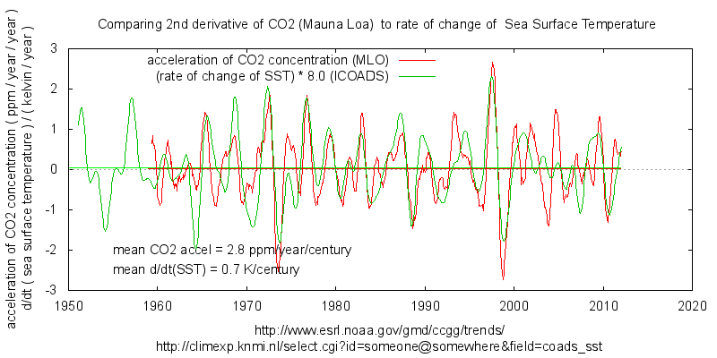
The following graph has been scaled to compare the longer, inter-decadal rise. It seems to match quite well on that scale too, including the post 1990 ‘pause’, though the record is too short for any such similarity in general tenancies to be regarded as statistically significant.
It should also be noted that this scaling shows a background d/dt(CO2) of 1 ppm/year around 1960 and 2 ppm/year post-2000. That can be regarded as another time-scale: centennial. The 800y lag in the ice core record deals with yet another time-scale: millennial. The latter also deals with a flip between two quasi-stable states of the climate system that shuts down a large proportion of life on earth. Thus direct comparison requires caution.
Each of these time-scales presents a different scaling factor of dCO2 and temperature. That seems to have got very little attention in this kind of discussion so far yet will be a key to identifying the processes involved.
The inter-annual relationship can be better estimated by going one step higher in differentials : dT/dt and d2/dt2(CO2). This is the same relationship, the high-pass properties of differentiation help to isolate the inter-annual variation. Since this has also has the annual cycle removed, it is in fact a bandpass filter centred on inter-annual periodicity.
The mean of both series also provides us with the scaling of dCO2 and temperature over the 60 period of the data.
As noted on the graph this provides inter-annual scaling of 8 ppmv/year/kelvin . This value is corroborated by isolating the largest inter-annual swing in the record around 1998.
https://climategrog.wordpress.com/?attachment_id=623
The half century scaling is 4 ppmv/year/kelvin
NOTE THE UNITS: this is ppmv/year/kelvin NOT ppmv/kelvin ,ie. it is that much every year, not overall. This is not the resulting equilibrium level of change but the rate of change.
Now if we look at a slightly longer filter which removes anything faster than 4 year variability we see a similar thing but note that the phase no longer aligns as closely. Here d2/dt2(CO2) lags dT/dt , particularly during the post-2000 pause where it is about 1.5 years where the main variability isolated by the filter has a period of about 10 years, where 2.5 years would put them back in phase.
This is the first indication of a move towards equilibrium. CO2 takes a first step towards being in phase with temperature rather than being orthogonal. This is significant for a couple of reasons.
1. It is in accordance with the kind of relaxation response that would result from Henry’s law and Feck’s law, relating to out-gassing.
2. It is first indication of the time constants applicable to the relationship. During the ‘pause’ there is already a significant shift towards the equilibrium phase response seen on the decadal scale.
The last graph also shows that a large proportion, though not all. the variability on the decadal scale can be attributed to temperature.
This leaves the question of how much of the centennial variation is due to out-gassing and how much to rising emissions. The available data is too short to properly answer this question but this kind of phase analysis can at least confirm the short term dCO2 dependency and gives the first clues as to the time constants of the system.
The averaged acceleration of CO2 over the record is 2.8 ppm/year/century. Warmists attribute this entirely to human emissions ( annual emissions being about twice the annual rise, so they discount out-gassing as negligible and conclude 50% is absorbed. )
However, if we have 8ppm/year/kelvin on inter-annual scale and conclude nothing significant on decadal scale that would imply CO2 equilibrates within ten years. Yet IPCC hypothesises this to be centuries if not millennial.
This is totally at odds with the record.
Mike,
The influence of temperature on CO2 levels is in ppmv/K not ppmv/K/time-unit.
The biosphere in general is absorbing more CO2 with higher temperatures and CO2 levels, thus not the cause of the increase in the atmosphere.
The oceans would be in dynamic equilibrium (steady state) at ~290 ppmv for the current ocean temperature, where ~40 GtC/year is the continuous input from the warm upwelling places in the tropics and ~40 GtC is the continuous uptake of CO2 at the cold polar sink places. Any temperature increase of 1 K is good for not more than ~8 (4-17) ppmv extra in the atmosphere:
http://www.ferdinand-engelbeen.be/klimaat/klim_img/upwelling_temp.jpg
Temperature gives a transient response of the ocean-atmosphere system, not a continuous influx of CO2 for a fixed step response of temperature.
At this moment there is a difference of ~3 GtC extra uptake by the oceans caused by the 110 ppmv extra CO2 pressure above equilibrium. Thus the oceans are a net sink for CO2, not a source.
The ~8 ppmv/K does apply to all periods over the past 800,000 years. Your ppmv/K/time must be adjusted for every period again and is even negative over the period 1975-1995 and 2000-current, that is 35 years of the past 55 years. It gets near zero over the 5000 years of warming during a deglaciation…
Ferdinand
Isn’t your 8 ppm/K calculated from the polar temperature swing? Global temp doesn’t vary that much.
“Mike, The influence of temperature on CO2 levels is in ppmv/K not ppmv/K/time-unit.”
No, that is the equilibrium relationship, not the dynamic one. If you present the calculations that you use to get your 8 ppmv/K it will be clear that it is not valid across all temperatures and thus does not apply to all regions. If ‘average’ regions are fairly stable it is regions that are more sensitive that will show up in the record and have greatest influence.
It is possible that there if covariance with other factors but the correlation of SST to dCO2 can not be dismissed as “noise”simply because it is inconvenient. This is the fallacy behind the whole AGW show: CO2 and temps both generally rise with time ; all the rest is ‘noise’.
The price of bananas has also general risen over that last 60 years, therefore bananas cause global warming ; deviations are ‘noise’ .
It’s like any relaxation response. There is an initial fast change ( the time derivative ) towards restoring equilbrium. Then there is the final offset that results from the change in the driving conditions.
It’s analogous to temps. A change in radiative “forcing” initially induces a *rate of change* of temperature. Then feedbacks coming to play and eventually the system settles to a new equilibrium with a temperature offset caused by the change in radiation.
With a hypothetical step change it is easy to see. In a real, dynamic, ever changing system it is a lot harder to separate the two.
Much of problem with exaggerated climate sensitivity to CO2 is due to exactly this failure to understand the difference between the two and the need to separate them.
Igl,
The short term change is ~5 ppmv/K for (global) seasonal and 4-5 ppmv/K for the 1-3 years variability. Where seasonal the NH extra-tropical forests are dominant, while for the 1-3 years variability the tropical forests are dominant (Pinatubo, ENSO).
For the 8 ppmv/K, the oceans are dominant over very long periods: multi-decennia to multi-millennia as can be seen in ice cores, be it that “temperature” in that case is based on d18O as “proxy” and mostly reflect the SH ocean temperatures where water from the ice cores originated. The Vostok ice core shows a quite linear correlation between CO2 and temperature:
http://www.ferdinand-engelbeen.be/klimaat/klim_img/Vostok_trends.gif
Mike, as explained above, the steady state (dynamic) equilibrium between oceans and atmosphere is exactly the same as for a static system. If you increase the temperature at all places, sources and sinks, the local pCO2 increases with ~8 μatm/K and thus the local influx or outflux changes accordingly. If you change the atmosphere with the same 8 ppmv, the original fluxes are restored and nothing happens with the CO2 levels in the atmosphere due to temperature anymore: that is again at the same (dis)equilibrium as before the temperature change:
http://www.ferdinand-engelbeen.be/klimaat/klim_img/upwelling_temp.jpg
The problem I see is that (too) many here try to explain a 110 ppmv increase from a +/- 1 ppmv natural variability caused by temperature variability which violates Henry’s law, while the elephant in the room, the 200 ppmv human emissions are ignored…
http://www.clim-past.net/9/367/2013/cp-9-367-2013.pdf
Igl,
The Annan work should imply that the 4 K increase caused about 100 ppmv increase or 25 ppmv/K. Seems rather high to me and above Henry’s law for seawater (maximum found in the literature of 17 ppmv/K), while vegetation is a net sink over such periods with expanding vegetation (area and density) with melting ice and higher temperatures…
But even so, that explains not more that 20 ppmv of the 110 ppmv increase over the past 160 years.
Oops, forgot the 4y filtered graph:
https://climategrog.wordpress.com/?attachment_id=254
What is astounding here us that nobody – sorry, shouts <i.NOBODY mentions OCO-2 – a direct measuring and purpose built asset for recording atmospheric CO2.which is giving the modelers at NASA the vapours to the point where they’re very obviously obstructing access to data.
Make of that what you will………………………..
There is no problem with the OCO-2 data, besides that one need to wait for at least a full year of data, before one can have any meaningful conclusion.
The seasonal changes are very huge, about an order of magnitude larger than human emissions, but the seasonal changes largely cancel out over a full year. Thus have some patience…
And your support for the assertion that “there is no problem with OCO-2 data” is ???
Other “A Train” resource satellites are routinely accessible and data is displayed days after a pass…. like Cloudsat
I’m afraid I can’t accept your proffered reasoning. Granted some folk without the requisite expertise might pounce on narrow results and misinterpret them – but – that actually applies in any remote sensing endeavor regardless of timescale and you should know that. It’s a time consuming and frustrating exercise + PITA to walk people through their errors and misinterpretations .
This simply stinks of obstruction and I shudder to think what contortions are happening behind the scenes.
I’d expect some “anomalous results” – for everybody – but the wholesale bust in circulation and distribution morphology already seen makes it look like this data is new and conflicts dramatically with present models – and is from that – of intense interest……
so – no… it’s obstruction – pretty much any other earth observation mission drops eye candy as soon as they can – to keep the trail of interest alive. The silence speaks volumes.
I’d add for the record that $280 million USD was initially spent on this state of the art CO2 mapper and that there;s a community of folk still being paid to gather and process that data …. what is going on?
avon,
Calm down… Indeed some primary results of the OCO-2 satellite are surprising, but the hype I have seen on some blogs that this refutes the whole AGW thesis, based on two weeks of data is largely overblown.
Take the quantities involved: human emissions currently are around 9 GtC/year or ~4.5 ppmv/year or 0.01 ppmv/day. Even if the satellite can focus on one spot for a longer view and most human emissions are concentrated is relative small areas, it will be a hell of a job to separate them from the natural variability. Which can be huge, if there is a lot of vegetation: plants respire during the night and take CO2 in during the day. On a average summer day the local diurnal change can be 150-200 ppmv…
To have some idea of the main sources and sinks over a year, one need at least one full year of data and preferentially several years, as we now have an El Niño year, which is quite different from an “average” year.
Ferdinand Engelbeen – So, are you saying the OCO-2 unadjusted data WILL be released BEFORE the Paris love fest? If so, we should all be patient. If not, we should be screaming bloody murder. GK
[snip – insulting – name calling – rephrase and resubmit -Anthony]
mods – sorry – click too soon …
What is astounding here us that nobody – sorry, shouts NOBODY mentions OCO-2 – a direct measuring and purpose built asset for recording atmospheric CO2.which is giving the modelers at NASA the vapours to the point where they’re very obviously obstructing access to data.
Make of that what you will………………………..
I make of that fact what I saw coming when I first heard of OCO-2. I knew that the very basis of modern climate “science” was erroneous and so they would not see what they thought they would see. I am surprised they let us see any data at all. But we all knew the climate models are heifer dust anyway.
@ferdinand meeus: “All known evidence shows that man is causing the increase”.
If by evidence you mean the same ‘evidence’ that has been manufactured to suit a predetermined political agenda, then I would agree.
But surely it can’t be “all known” evidence? Salby alone has provided an abundance of counter-evidence against the proposition that we humans are driving the increase.
To that you could add Tom Quirk, Humlum, Francey, Segalstad, Jaworowski, and many others who disagree for reasons explained thoroughly in the peer-reviewed literature.
Richard,
Some observations are quite solid and global: CO2 levels, δ13C levels, 14C bomb spike decline, oxygen balance,… All of them point to humans as origin of the increase…
Salby and many others, including Allan here again, try to extrapolate the trend in CO2 from the noise around the trend, but in this case it is proven (from the opposite δ13C changes) that the variability around the trend is caused by the influence of temperature on vegetation, but the trend is NOT caused by vegetation, as that is a net, increasing sink for CO2 (proven by the O2 balance), the earth is greening…
So variability and trend have nothing to do with each other: different causes at work. The obvious cause for the variability is temperature variability. The obvious cause for the trend is human burning of fossil fuels…
As they say: even one fact can destroy the nicest theory. In this case all theoretical non-human sources for the CO2 increase fail one to many observations…
“Salby alone has provided an abundance of counter-evidennce…”
Salby, sadly, has produced nothing in terms of evidence. He has produced some hand–waving videos. It seems quite clear at this stage that he is not going to publish anything , even on the internet, that can be scrutinised.
He has generated some discussion , which is useful.
OK Ferdinand – that’s three times you have mischaracterized what I have said here.
Bad boy! No alcohol for you for the remainder of the day!
Mike, I think it’s a little unfair to say that all Salby has contributed nothing more than hand-waving. He has at the very least shown that atmospheric CO2 and human emissions appear to be following different growth-rates (i.e. his 300% argument).
Ferdinand, vegetation might be a net-sink, but I was talking about changes in ocean biology which would also be depelted in C13. Non-biogenic ocean out-gassing would increase dC13 since it has per mil values ranging from -7 to 1.5 but if there were changes in ocean biology, say an increase in the productivity of phytoplankton for example, that would decrease dC13, since the per mil value of phytoplankton is much lower at around -26. I am suggesting that human emissions are not decreasing dC13, indeed they must be to some degree, but a certain percentage of that decrease might be coming from changes in ocean biology.
And my position is not new – this note to Ferdinand posted in 2008.
http://wattsupwiththat.com/2008/12/17/the-co2-temperature-link/#comment-67050
[excerpt]
Hi Ferdinand and Richard,
I think it is safe to say that Ferdinand is convinced that the recent increase in atmospheric CO2 is definitely caused by fossil fuel combustion, while Richard and I regard this point as debatable.
The oco2 Data is freely available here-
ftp://oco2.gesdisc.eosdis.nasa.gov/data/s4pa/OCO2_DATA/
Thanks D.I. – I’d missed that – the directory structures I looked at were linked from the mission pages and near empty…
Time to engage with the gridding API then
“I suggest with confidence that the future cannot cause the past.”
LOL, I should certainly hope so! Mind you, the way climate science is behaving with respect to this debate (i.e. Consensus) anything goes I suppose.
Allan MacRae’s argument is one of the counter arguments to “CO2 does it all”, and a very good one at that. There is also the counter argument that CO2, on net, does not warm the surface at all and cools the atmosphere rather than heats it. However, all skeptics who are paying attention, even the luke-warmers, can see that the alarmists have developed a religious cult that claims they know that CO2 drives the temperatures on earth. (and they will adjust measurements to prove it!)
It is high time all skeptics take a real look at the basic physics of the argument over CO2’s role. The Scottish Skeptic once observed that it may be bad public relations and tactics to look at the issue of CO2 causing warming but in the long run the truth of the matter demands close inspection of the issue.
Some of us believe as we were taught decades ago that the climate of the planet is due to gravity, mass of the atmosphere, conduction, convection, advection, the oceans, H2O in the atmosphere, and of course insolation of energy from our local star. It is all the gasses of the atmosphere plus the ocean that is the “driver” of our climate.
I hope to see more posts on this issue in the future here.
“Some of us believe as we were taught decades ago that the climate of the planet is due to gravity, mass of the atmosphere, conduction, convection, advection, the oceans, H2O in the atmosphere, and of course insolation of energy from our local star. It is all the gasses of the atmosphere plus the ocean that is the “driver” of our climate.”
Good to see that others have the same recollections as me. It was all about the density of trhe atmosphere in those days and any radiative imbalances were corrected by adjustments to convective overturning.
http://www.public.asu.edu/~hhuang38/mae578_lecture_06.pdf
It is true that surface radiative imbalances are compensated for by adjustments to convective and evapotransporation/condensation processes. However, that does not disprove that the atmospheric greenhouse effect is caused by radiation absorbing gases (H2O and CO2 mainly). The extra surface temperature effect is due to the increase in the average altitude where radiation to space occurs, combined with the effective lapse rate, and the fact that the effective temperature of the average location of radiation to space has to radiate the absorbed solar radiation. The increase is due to the fact that convective and evapotransporation/condensation processes do not radiate to space, they simply carry the energy to a greater altitude than the surface, where the energy is transferred to gasses (H2O and CO2 mainly) that then radiate to space. The O2 and N2 do not significantly radiate at temperatures in the atmosphere, so any mechanism that moves energy other than radiation have to be eventually radiated by the H2O and CO2. This argument does not show how much an increase in CO2 will increase surface temperature, since change in water vapor may result in a negative feedback due to cloud changes, and thus average albedo.
replace gravity with gravity collapse. Add: solar variation, solar system orbital variations, ocean circulation, tilt variations, geophysics.
In reply to:
William,
The cult of CAGW sponsored research is so predictable.
The cult of CAGW reduces either the amount of water available at the root of the plant which reduces the amount of available nitrogen or have reduced the natural nitrogen producing bacteria at the root of the plant by the isolating the plants in a greenhouse for the enhanced CO2 experiment. i.e. The cult of CAGW fudges the analysis to get the result(s) they want. (i.e. That CO2, a gas that is essential for life of this planet, is a poison and causes dangerous warming.)
The increase in atmospheric CO2 is unequivocally beneficial for the biosphere due to effect of CO2 on plants and due to the high latitude warming. There has been almost no warming in the tropical region which supports the assertion that cloud cover in the tropics increases or decreases to resist forcing changes. The majority of the warming has been in high latitude regions which has caused the biosphere to expand.
C3 plants (all plants except for grasses) lose roughly 40% of their absorbed water due to trans-respiration. When atmospheric CO2 rises, C3 plants produce less stomata on their leaves (note the optimum CO2 level for plants is 1200 ppm) which reduces the amount of water they lose due to trans-respiration.
The principal source of nitrogen for plants is nitrogen fixing bacteria which live at the root of the plant.
Less stomata on plant leaves results in less water loss which results in more water at the plant roots for the nitrogen fixing bacteria.
http://www.azocleantech.com/details.asp?newsID=4587
http://www.sciencedaily.com/releases/2003/05/030509084556.htm
http://news.nationalgeographic.com/news/2009/07/090731-green-sahara.html
http://www.omafra.gov.on.ca/english/crops/facts/00-077.htm
https://secure.ntsg.umt.edu/publications/2013/BRGT13/BastosJGR2013.pdf
From the paper
>>
[2] Anthropogenic CO2 emissions from fossil fuel burn-
ing and land-use change have been increasing since the
1960s. Each year, about half of anthropogenic emissions
remain in the atmosphere, being the remaining half absorbed
by land and oceans sinks [Le Quéré et al., 2009]. In the
last decades, these sinks presented an increasing strength but
also considerable interannual variability.
>>
So the sinks presented increasing strength. One reason maybe that the strength of the ocean sinks was weakened by ever increasing out gassing. Since the stabilisation of temperatures the ocean sink is comparatively stronger.
It’s always a net absorber, but now absorbing a stronger proportion of emissions that the latter part of 20th c. This is driven on one side by the higher atm CO2 and on the other by the plateau in temperatures:
This is consistent with temp vs dCO2 relationship on inter-annual and decadal scales Some proportion of the steady 2ppm/year is also probably attributable to centennial scale out-gassing.
Mike,
If one assumes that the ocean-atmosphere system is a simple first order equilibrium process, one can calculate the sink rate of the system based on the on the emissions and the overall net sink rate and steady state level for each year based on the SST temperature of that year. Here I have done that for the period 1960-2012 (the last year of the emissions inventory):
http://www.ferdinand-engelbeen.be/klimaat/klim_img/dco2_em6.jpg
Temperature has a high correlation with the CO2 rate of change variability, but has a bad correlation with the trend: the correlation 1975-1995 is even negative and 2000-current is zero to slightly negative, depending of which temperature trend one uses. That is for 35 of the 55 years. The correlation between accumulated human emissions and the increase in the atmosphere on the other side is almost perfect:
http://www.ferdinand-engelbeen.be/klimaat/klim_img/acc_co2_1960_cur.jpg
Which points to a simple linear process which is too slow to coop with the pace of human emissions…
“The correlation between accumulated human emissions and the increase in the atmosphere on the other side is almost perfect:”
Hey Ferdinand. You’ve plotted two cumulative integrals: CO2 and temp ( which is accumulation heat energy ). They are roughly straight lines , so obviously if you scale and shift them of course the correlation is “almost perfect”. It meaningless.
You need to look at the higher derivatives to reveal the variations in the data. And when you do, you see what the relationship is.
No idea what your first graph is about because you don’t explain how you do you calculations and what assumptions you are making. Pretty meaningless just banging up a graph like it proves something.
Again, if you present the calculations that you use to get your 8 ppmv/K it will be clear that it is not valid across all temperatures. You avoid addressing that.
Sorry Mike,
I have plotted one integral: accumulated emissions against direct measurements of CO2 in the atmosphere.
As both are increasing slightly quadratic in the atmosphere, the net sink rate is slightly quadratic increasing too and the net result in the derivative are near straight lines.
Here the plot of the accumulated emissions, temperature and increase in the atmosphere.
http://www.ferdinand-engelbeen.be/klimaat/klim_img/temp_emiss_increase.jpg
That shows that in the 19745-1975 period the temperature was slightly decreasing while emissions increase and CO2 in the atmosphere increases in ratio to the emissions. What also is visible is that the variability of temperature has very little influence on the variability of the CO2 increase in the atmosphere.
Looking at the derivatives of the sum of two influences where one has little influence on the CO2 trend and huge variability and the other shows a huge trend but no measurable variability in the atmosphere doesn’t give you any answer about the cause of the increase in the atmosphere, it only shows the cause of the variability, not of the trend. In this case is looking at the derivatives highly misleading, as the trend is not caused by the same process that causes the variability, the latter has a negative trend (growing vegetation with increasing temperatures).
My plot of the theoretical CO2 rate of change is quite simple: for every year the net sink rate is calculated as the ΔpCO2 between CO2 level measured for that year and the equilibrium level for the temperature of that year (base 290 ppmv in 1900 + 8 ppmv/K), multiplied by the sink factor (2.15 ppmv / 110 ppmv). That is subtracted from the emissions of that year. That is all.
The 8 ppmv/K is what the ice cores show over the past 800,000 years and is in the middle of the range given for Henry’s law for the solubility of CO2 in seawater. The calculation used for the correction of the pCO2 measurements for the change in temperature between seawater inlet and automated equilibration measuring device is here:
(pCO2)sw @ Tin situ = (pCO2)sw @ Teq x EXP[0.0423 x (Tin-situ – Teq)]
the explanation is at:
http://www.ldeo.columbia.edu/res/pi/CO2/carbondioxide/text/LMG06_8_data_report.doc
Ferdinand…….How come Bart is not commenting here?
Bart doesn’t know what more to say that he hasn’t explained over and over and over again. Ferdinand is still making his same old static arguments. I mean, there are still discussions going on over the pitifully stupid, ignorant, and ridiculous “mass balance” argument. I might as well waste my time trying to teach my dog Latin.
Atmospheric CO2 is set by the ocean interface, and the rate of change of CO2 in the surface oceans is determined by the temperature dependent net imbalance between upwelling and downwelling waters. Human inputs are pitifully small compare to these flows.
That is what is happening. That is what people will eventually realize when emissions and atmospheric concentration have diverged starkly enough from affine similarity. Until then, Ferdinand is a rock star to the lemming contingent, and I have better things to do.
Bart and Ferdinand can agree on one thing: there is no evidence showing any global harm resulting from the rise in CO2. As far as anyone knows, CO2 is completely harmless.
CO2 is also a net benefit to the biosphere, which is measurably greening due to the increase. It is still just a tiny trace gas; within a tenth of a percent, there is no CO2 in the air at all.
The 31,000+ OISM co-signers were correct: CO2 is harmless, and beneficial to the biosphere.
That’s what really matters, no? The climate alarmist contingent is flat wrong when they try to demonize “carbon”. They just can’t admit that what they’ve taught everyone for the past few decades was simply wrong.
Joel,
Bart still hasn’t figured out that the steady state level for the CO2 system between oceans and atmosphere is exactly the same for the dynamic system it is as it is for the equilibrium between a static sample of seawater in a lab and the air above it after some time…
Neither has he figured out that it is impossible to have an observed 4-fold increase rate in the atmosphere (caused by the 4-fold increase of human emissions) with a 3- or 5-fold increase in natural carbon cycle, neither that such an increase would violate about all observations…
Ferdinand, this is as dumb as your unthinking acceptance of the ridiculous “mass balance” argument. In a system in which equilibrium is established by a dynamic imbalance, all that is needed for a change is a net imbalance between input and output. As a result, sensitivities generally have a temporal dependence. And, that is why the sensitivity of atmospheric CO2 to temperature is in ppmv/K/unit-of-time.
There is no doubt about it. It isn’t even a close call. You are wrong.
Bart,
It seems quite difficult for you to accept that a dynamic imbalance not only is influenced by temperature at the ocean side but also by the partial pressure at the atmosphere side. Thus while temperature has a short living ppmv/K/unit of time influence, the resulting in/decrease in the atmosphere reduces the ppmv/K/unit of time until the original in/out fluxes are restored and the end result is in ppmv/K.
Nope. I’ve shown this in exhaustive detail in a post on Dr. Curry’s blog. You are absolutely wrong.
Bart,
Your posts here and at Curry’s only shows that while you may have a lot of knowledge on high frequency processes, you have not the slightest idea how a simple first order dynamic physical process works. It is beyond ridicule that a temperature increase at the upwelling(/downwelling) side would produce a continuous in(/de)creased in(/out)flux of CO2 without response from the increased CO2 pressure in the atmosphere. It is complete nonsense and only shows that you don’t know where you are talking about…
I am extremely well versed, and experienced, in all types of feedback designs, Ferdinand, from those acting on microsecond levels to centuries long.
You are totally out to lunch. If the CO2 content of the surface oceans increases, then the corresponding increase in the atmosphere is ineluctable. The equalizing of partial pressure is precisely the mechanism by which such an increase is enforced. Far from limiting it, it is the cause of it.
Bart,
The fact that you don’t even consider the feedback from the increase of pCO2 in the atmosphere in your formula to an increase in temperature only shows that either you are “forgetting” even the basic rules of feedback control if that is counter your theory, or you have not the slightest experience with that kind of physical/chemical processes.
The influx of CO2 from the upwelling sites is directly proportional to the pCO2 difference between oceans and atmosphere.
The pCO2 of the oceans for a given concentration is governed by temperature at not more than 8 (4-17) μatm/K change. That means that for a change of ~8 ppmv/K in the atmosphere the original influx is restored, all other influences (concentration, upwelling amount, wind speed,…) being constant.
The same happens for an increase in CO2 concentration in upwelling or total upwelling or a combination with temperature: in all cases a change in CO2 level in the atmosphere will counter the change until a new steady state is reached, together with similar – opposite – changes at the downwelling sites.
Think, Ferdinand. If the oceans are becoming more and more enriched with CO2 from upwelling and failure to downwell in equal measure, then the atmosphere will become more enriched, too.
Think a little further Bart:
If the upwelling waters are enriched with CO2, the pCO2 of the oceans will increase and the ΔpCO2 with the atmosphere increases. That results in more influx. The increased influx will result in an increased pCO2 of the atmosphere, which reduces the ΔpCO2 between atmosphere and increased pCO2 of the ocean surface at one side and increases the ΔpCO2 at the sink side. That goes on until a new steady state is reached:
http://www.ferdinand-engelbeen.be/klimaat/klim_img/upwelling_incr.jpg
Even an extreme 10% increase in upwelling, either by total upwelling or concentration (for which is no evidence at all) does level off at some 30 ppmv extra in the atmosphere.
You have a strange idea about CO2 “piling up” at the ocean surface: the pCO2 of the upwelling waters is what is measured as maximum 750 μatm for the temperature (~30°C) at the equatorial surface and the (~40 GtC/year) flux into the atmosphere is proportional to the 750-400 μatm difference between ocean surface and atmosphere.
If there was no more upwelling, the pCO2 of the ocean surface would go down to 400 μatm, even at the equatorial seawater temperature, in equilibrium with the atmosphere and the influx would stop. You need the upwelling to maintain the 750 – 400 μatm pCO2 difference and the resulting influx.
CO2 doesn’t “pile up” at the upwelling zones, it simply gives more influx when the concentration or the temperature or both increase. That is fully compensated for by the increase of pCO2 in the atmosphere after some time.
It would, IF the oceans only had a step in concentration. But, with continuous upwelling of CO2 enriched waters, and reduced downwelling of CO2 due to temperature rise, the ocean concentration is continuously increasing. The atmospheric CO2 will continuously increase as well.
Bart,
Of course there must be a continuous upwelling and a continuous sink of CO2, or there is simply no “steady state” and the ocean-atmosphere system would be in rapid equilibrium (within a year). It is because there is upwelling at high temperatures near the equator and downwelling near the poles that makes that there is a dynamic equilibrium or disequilibrium, depending of the variability of the upwelling and sinks and external factors like human emissions…
But, with continuous upwelling of CO2 enriched waters,… the ocean concentration is continuously increasing.
Sorry, but that is a step too far: a continuous upwelling of CO2 enriched waters has a fixed concentration and thus a fixed pCO2 at a fixed temperature and only gives an initial increased influx of CO2 in the atmosphere if the concentration or temperature or both increased. In all cases that is countered by the increase of CO2 in the atmosphere. CO2 doesn’t pile up at the ocean surface, it is released in ratio to the ΔpCO2 with the atmosphere. If the ΔpCO2 with the atmosphere decreases by the increased pressure in the atmosphere, the CO2 influx get reduced, no matter how much CO2 is in the ocean: that part of CO2 remains in the ocean surface.
Or are you talking about a continuous increasing concentration of CO2 in the upwelling, for which is not the slightest indication (neither for a step in concentration)?
For a fixed ocean upwelling (at a fixed CO2 concentration) and downwelling water flow, a temperature increase will give an increase of 8 ppmv/K CO2 in the atmosphere in a transient response of the dynamic process. That is all.
Game, Set, and hopefully.. Match.
Now, we ought to be able to encourage technological rather than religiose solutions to mankind’s unhealthy overdependency on hydrocarbon fuels ….
TonyN
Please explain what is “unhealthy” in our use of hydrocarbon fuels without which modern medicine would be impossible.
And in what way do we have an “overdependency on hydrocarbon fuels” when the use of hydrocarbon fuels has done more to benefit human kind than anything else since the invention of agriculture and there are no known and sufficient alternatives?
Richard
“I suggest with confidence that the future cannot cause the past.”
That remains to be seen.
Future computer models may indeed show that future lags past, as the models were built on a simple “cart before the horse” strategy. By offsetting the feedback mechanism until it is precisely centered on this moment in time, future catastrophe is avoided… though at great cost… as all flows of energy, appropriation and precious human time, even the apparently unquenchable curiosity of Willis Eschenbach, are stretched around and asymptotically into the singularity of this moment until every statistic becomes a simple gainsay of the central argument… is CO2 lagging behind T?
“Yes it is. No it isn’t. ‘Tis. ‘Tisn’t … … … Ding! Thank you!”
Cheer up everyone! Things may be getting worse at a slower rate.
Similar point made here:
http://www.newclimatemodel.com/evidence-that-oceans-not-man-control-co2-emissions/
It is not necessary to raise the temperatutre of the entire oceans to achieve more CO2 outgassing. Just more sunlight into the water beneath the subtropical high pressure cells will do the trick.
Those cells seem to expand or contract in line with variations in global cloudiness as a result of changes in solar activity via a mechanism that I have set out previously.
The ToA solar constant is 340 (+10.7/- 11.2 footnote 1) W/m^2 as shown on the plethora of popular heat balances/budgets. Collect an assortment of these global energy budgets/balances graphics. The variations between some of these is unsettling. Some consensus. BTW additional RF due to CO2 1750-2011, about 2 W/m^2 spherical, 0.6% of ToA.
In 24 hours the entire globe rotates through the ToA W/m^2 flux collecting heat of 1.43E19 Btu/day
Suppose this heat load were absorbed entirely by:
the air:
Daily temperature rise: 5.25 °F / day
Due to RF of CO2: 0.03 °F, 0.6%.
Obviously the atmospheric temperature is not increasing 5.25 °F per day (1,916 °F per year). There are absorbtions, reflections, upwellers, downwellers, LWIR, SWIR, losses during the night, clouds, clear, yadda, yadda.
the oceans:
Daily temperature rise: 0.00462 °F / day (1.69 °F per year)
How would anybody notice?
by evaporation:
Portion of ocean evaporated: 4.76 ppm/day (1,737 ppm, 0.174%, per year)
More clouds, rain, snow, etc.
Oceans, clouds and water vapor soak up heat several orders of magnitude greater than GHGs put it out. CO2’s RF of 2 W/m^2 is inconsequential in comparison, completely lost in the natural ebb and flow of atmospheric heat flux. More clouds, rain, snow, no temperature rise.
Footnote 1: Journal of Geophysical Research, Vol 83, No C4, 4/20/78, Ellis, Harr, Levitus, Oort
also BSME & PE
Since Ray is a professional engineer, I would expect him to have ready access to something better than a running mean as a filter. It’s a shame he did not update this work for this post. The data continues to fit well since 2005 and the ‘pause’ in both datasets is interesting.
I think if you are skeptical of the “tipping point” you would have to be skeptical if humans produce co2 could warm the earth at all in the long term.
I’ve linked to my analysis several times on WUWT. Anyone can plot the 12 month change in atmospheric CO2 and the 12 month change in temperature on the same chart. The result is indecipherable, because the series are very noisy. Smooth both with the same filter, say a 12 month moving average, and the data since the start of the Mauna Loa series absolutely screams at you that temperature leads CO2, by a small number of months.
This is exactly what any sane person would expect, as short term temperature rises decrease the solubility of CO2 in the oceans.
This has nothing to do with whether CO2 causes 3.7 Wm-2 extra heat per doubling. That result isn’t seriously challenged.
If anything, this data supports a positive feedback (not captured in ECS) which will raise atmospheric CO2 in the long term as temperatures rise.
http://Www.robles-thome.talktalk.net/carbontemp.pdf
[Link fixed. ~mod.]
RERT
One would also expect to see longer term CO2 responses to naturally induced climate variations such as that from MWP to LIA to date.
It is seriously challenged that our CO2 would necessarily cause 3.7 Wm2 extra ‘heat’ per doubling.
The evidence is that any extra ‘heat’ from GHGs simply distorts the lapse rate slope to the warm side in ascending air and to the cool side in descending air for a zero net effect at the surface.
One needs to know some non radiative meteorology to appreciate that.
RERT – your link does not work.
BTW, it is NOT just “the solubility of CO2 in the oceans.”
Look at the AIRS video.
[Link fixed. ~mod.]
Thanks to mod and RERT.
RERT,
Your link doesn’t work, but besides the “normal” ~8 ppmv/K influence of temperature (4-5 ppmv/K in short term), the oceans can’t give you 110 ppmv (70 ppmv since Mauna Loa started) increase from a 0.6 K temperature increase. That violates Henry’s law for the solubility of CO2 in seawater.
In this case, the short term variability is caused by temperature, but the trend is NOT caused by temperature, it is caused by human emissions, which are twice the observed increase in the atmosphere…
You are correct. There is indubitably a positive gain from temperatures to CO2. If, in turn, there is a net positive gain from CO2 to temperature, then there is a positive feedback of a type which cannot be stabilized merely by T^4 radiation.
Thus, the Earth would have reached a saturation point of high CO2 and temperature eons ago. As it did not, and shows no signs of doing so, there cannot be a net positive gain from CO2 to temperature, i.e., increasing CO2, in the present state of the climate system, does not increase surface temperatures.
“eons ago?”
…
Hasn’t TSI changed over millions of years as our yellow G2V star has evolved?
http://www.robles-thome.talktalk.net/carbontemp.pdf
I’ve tried again with the link.
Stephen –
CO2 lagging temperature long term is consistent with the ice core data which shows 800 year lag quoted between temperature rises and CO2. You can also look at the law dome CO2 record and see CO2 fall during the LIA. Temperature does drive CO2. This says *nothing* in my view about whether CO2 causes greenhouse heating, which I believe it does.
Allan – no, it’s not just the solubility of CO2, but I believe this is a major factor, and a very obvious one.
Ferdinand – I didn’t for a minute suggest that all atmospheric CO2 addition was from temperature changes. But temperature does affect CO2 positively.
Bart – no, there are just other factors which are not identified.
Temperature leading CO2 is just meme which gets attacked because it is in the ‘too complicated’ bucket for the CAGW crowd for their propaganda purposes.
RERT says:
This says *nothing* in my view about whether CO2 causes greenhouse heating, which I believe it does.
I believe it does, too. I say ‘believe’ because I’ve never found any data or charts showing that ∆CO2 is the cause of ∆T. So the global warming effect of CO2 must be too small to measure.
But I have lots of charts like this showing that ∆T causes ∆CO2:
[click in charts to embiggen]
http://www.brighton73.freeserve.co.uk/gw/paleo/400000yearslarge.gif
Here’s a longer time frame:
http://upload.wikimedia.org/wikipedia/commons/8/82/Past_740_kyrs_Dome-Concordia_ice_core_temperature_reconstructions.png
And a much shorter time frame:
The alarmists got causation backward. No wonder their conclusions are wrong.
Stealey, could you please show us the spike in T that caused the CO2 to go from 280 ppm to 400 ppm?
http://lafenergy.org/essays/figs/Co2-temperature-plot.png
Jackson,
Your chart shows a large rise in CO2. But global T has been flat for almost twenty years.
I rest my case. ☺
1) “But I have lots of charts like this showing that ∆T causes ∆CO2:” …
…
Good, please show us the chart that shows the ∆T that has caused the CO2 to go from 280 to 400 ppm.
..
2) “All the available measurements show that T is the cause, and CO2 is the effect.. ”
…
Good, please show us the T that caused the CO2 to go from 280 to 400 ppm.
…
3) “I rest my case.” Why do you rest your case when evidence disproves your “case?” In the past 18 years, you claim “global warming has stopped” That means ∆T is zero for the past 18 years. But in the past 18 years CO2 has risen more than 35 ppm. Why has CO2 not followed T for the past 18 years ?
RERT @ June 14, 2015 at 2:03 pm
“…no, there are just other factors which are not identified.”
There may, indeed, be other factors. But the net effect of those other factors would have to be of a sort which made the aggregate feedback negative. The end result is the same – in the present state of the climate system, net influence of CO2 concentration on surface temperatures must be small.
Have we not seen essentially no temperature rise during the past roughly two decades, while CO2 levels rose an additional 33% above what is assumed to be the pre-industrial equilibrium? Mathematically and observationally, AGW is a dud.
Joel D. Jackson @ June 14, 2015 at 2:50 pm
“Why has CO2 not followed T for the past 18 years ?”
Because CO2 does not track T. The rate of change of CO2 tracks T. And, it has kept pace quite well for the past 18 years.
http://www.woodfortrees.org/plot/esrl-co2/from:1979/mean:12/derivative/plot/uah/from:1959/scale:0.22/offset:0.14
The arrow of causality is clearly in the direction of temperature driving the rate of change of CO2. When you integrate the rate of change, you get the quantity itself:
http://www.woodfortrees.org/plot/esrl-co2/from:1979/mean:12/plot/uah/from:1959/scale:0.22/offset:0.14/integral/offset:338
Bart, then do you agree with me when I say that Mr Stealey’s statement that ” ∆T causes ∆CO2 ” is incorrect?
…
I am under the impression that ∆CO2 and dCO2/dt are two different things.
Bart, I also have a question for you. In the past 18 years the change in T has been zero.
In the past 18 years the dCO2/dt has been about 2 ppm per year.
…
if dCO2/dt = 2 ppm/yr
and T-Teq = 0
…
What is your constant of proportionality for the past 18 years?
Jackson,
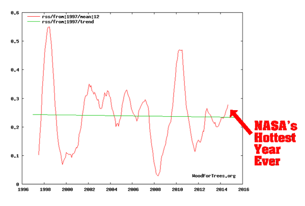
I said I rest my case. Since you have now changed the subject to a differnt kind of chart, my points (and charts) stand. Silence is concurrence, as they say.
Now, I’m not sure exactly what you’re angling for, but maybe this will fit the bill:
http://www.co2science.org/education/reports/co2benefits/figures/Figure8.gif
CO2 is harmless, and it is beneficial to the biosphere. More is better, at both current and projected concentrations.
Next, you have a problem, this time with your #2 question. Why don’t you quote my words? Is it because then you can erect your strawman argument, and then argue with that? Or is it because you claim to not cut and paste? Whatever the reason, what I said was that all the available measurements show that T is the cause of the rise in CO2. Got a problem with that? If so, show me a chart that verifies that CO2 is the cause of (non-existent) global warming. Make sure it isn’t the typical alarmist overlay chart. Show causation, like I did. But I don’t think you can.
I explained that there are no measurements for that, like there are for T causing CO2. I also wrote that I *believe* that CO2 is the cause of some minuscule warming. It’s my belief, because there aren’t any charts or measurements that show that, like there are showing that global ∆T is the cause of ∆CO2. I have plenty of those. Ask, and I’ll post more.
That’s hard for you to accept, I can see. Because you folks are always trying to demonoze “carbon”. Why? Because that’s the misinformation you swallowed hook, line and sinker. You believe that CO2 is a problem. But you are incapable of producing any testable measurements to support your belief. It’s your religion.
Yes, I rest my case. You lose, because you cannot produce falsifying information. Try to find a chart contradicting what I showed in the 3 charts above. On time scales from a few years, to hundreds of millennia, ∆T causes ∆CO2. You cannot accept that, because if you did your whole belief system would be in disarray.
It must be hell trying to convince yourself that the most benign century since the MWP has justt passed, and there is still no indication of any runaway global warming, or accelerating sea level rise, or disappearing Arctic ice, or vanishing Polar bears, or any of the other evidnce-free, measurement-free globaloney nonsense you believe in. You just believe, because that’s your new religion. Facts don’t matter. Facts like this just get in your way:
http://4.bp.blogspot.com/-lPGChYUUeuc/VLhzJqwRhtI/AAAAAAAAAS4/ehDtihKNKIw/s1600/GISTemp%2BKelvin%2B01.png
To sum up, the planet is measurably GREENING due to the rise in CO2:
http://www.drroyspencer.com/wp-content/uploads/co2_growth.jpg
Even Scientific American knew that, before it was bought by foreigners with an agenda.
And of course, fossil fuels have been incredibly beneficial:
Current CO2 levels are the lowest they’ve been in geologic history. The biosphere is starved of that harmless, beneficial trace gas, which has been up to TWENTY TIMES (20X) higher in the past — without ever triggering runaway global warming:
http://2.bp.blogspot.com/_cHhMa7ARDDg/SoxiDu0taDI/AAAAAAAABFI/Z2yuZCWtzvc/s1600/Geocarb%2BIII-Mine-03.jpg
But once you start to admit that, skeptics win the debate. Which is all about demonizing CO2 — a trace gas that is every bit as essential for life on earth as H2O.
You’ve painted yourself into a corner: you can’t admit that CO2 is harmless. So you frantically search for anything you can find to claim it’s not good for plants, etc. — as preposterous as that sounds to rational folks. You’re being hopelessly confused by your confirmation bias, rejecting anything that doesn’t support your new religion.
There’s a way out of your conundrum. Just stick with testable evidence and verifiable data and measurements. Answer questions for a change, instead of always asking but never answering. Because if you start answering questions… there goes your belief system. The climate alarmist crowd never wants to answer questions. Your belief is logically and scientifically unsupportable. The Real World is busy falsifying everything you believe:
All the wild-eyed arm waving over a *tiny* 0.7ºC wiggle, over a century and a half, is ridiculous to rational skeptics. It’s crazy, really. That is as close to flat as anything in the temperature record. But that’s what you hang your hat on! You may believe it’s a problem, but to scientific skeptics that just looks silly.
“I also wrote that I *believe* that CO2 is the cause of some minuscule warming. It’s my belief, because there aren’t any charts or measurements that show that, like there are showing that global ∆T is the cause of ∆CO2.” ~ dbstealey
Mr. Stealey, that whole comment from which I quoted a tiny bit was a very good one. I do appreciate you taking the time to interact on this thread, it has been gratifying to see.
I must tell you that I think CO2 does not even cause minuscule warming but we can put that aside for another day and both of us agree there is no measurable warming by CO2 that can be shown. And that, my friend, puts an end to the alarmist claptrap. CO2 as “driver” of climate is a dead end that is preventing mankind from getting on with the job of trying to understand the climate. (or the “weather machine” as we called it back in the day)
T-Teq is not zero, Joel, or David Socrates, or whatever your latest nom de plume is. Only one person could be so dumb as to keep getting that rather important detail wrong, and continue harping on it like he had something useful to say.
Tell me, why exactly do you keep changing your screen name?
Bartemis,
Yeah, that looks like “David Socrates”, doesn’t it?
That would explain a lot. It’s hard to believe someone could be that ignorant of the basics.
=======================
Mark Stoval, thanks for that. I don’t know for certain, but I’ve read the majority of Lindzen’s papers, and I defer to his greater knowledge. Whether CO2 does or doesn’t cause warming is almost exactly the same thing. We can’t tell either way because there are no measurements.
Bart:
Because CO2 does not track T. The rate of change of CO2 tracks T. And, it has kept pace quite well for the past 18 years.
Of course, CO2 does track T with a pi/2 lag on short term, it is a transient function. It has done that for at least 800,000 years, except for the past 160 years, but it still does that for the small variability of CO2 around the human caused trend.
And dCO2/dt tracks dT/dt with a pi/2 lag, which integral gives a small increase of CO2 of ~5 ppmv over the past 55 years.
dCO2/dt tracks T without lag because taking the derivative shifts dCO2/dt pi/2 back in time compared to CO2 and thus synchronizes with T, but that has no physical meaning.
That is gibberish, Ferdinand. Why you insist on writhing through such logical contortions to avoid accepting the obvious is beyond me.
Bart,
The response of CO2 to an increase in temperature of the oceans (or any other liquid) is a transient function, as you can learn from any textbook of physics:
http://www.ferdinand-engelbeen.be/klimaat/klim_img/upwelling_temp.jpg
A step response in temperature will give a fast response in extra CO2 influx at the upwelling zones and reduced outflux at the sink zones. That leads to an increase of CO2 in the atmosphere, which zeroes out when a new steady state is reached at ~8 (4-17) ppmv extra in the atmosphere. Then the increase stops. There is no way that a small permanent offset in temperature against an arbitrary baseline can give a fixed influx of CO2 without reaction from the increased pressure in the atmosphere on the influx and outflux.
It is mathematically proven by Paul_K that a sinusoidal change in temperature for any frequency is followed by sinusoidal change of CO2 with a pi/2 lag, as long as the system response is slow enough, which we may assume in this case:
http://bishophill.squarespace.com/blog/2013/10/21/diary-date-murry-salby.html
second page, 4th comment.
Thus any fixed change in temperature in this dynamic system between oceans and atmosphere gives a fixed change of CO2 in the atmosphere with a lag, as is proven over the past 800,000 years of reliable measurements.
If you take the derivative from the CO2 level, you shift the sinusoid pi/2 back in time, which makes that dCO2/dt changes are in perfect alignment with T changes. That is normal, as T changes are the cause of the initial rise in CO2 rate of change. But integrating T to obtain CO2 has no physical meaning, as CO2 is not the integral of T, it is the transient integration towards the new equilibrium, it is the integral of dT/dt which with some factor will give the amount of extra CO2 in the atmosphere.
dT/dt has no slope and only a slight offset from zero, which gives some 0.6°C increase in the period 1960-2012 when integrated and accordingly some 5 ppmv CO2 extra in the atmosphere. That is all:
http://www.ferdinand-engelbeen.be/klimaat/klim_img/temp_co2_der.png
The whole slope of dCO2/dt is caused by the near twice as high dCO2(em)/dt human emissions over the full period, not by temperature.
No, Ferdinand. Such a high pass response would necessarily produce readily observable phase distortion, which is entirely absent.
This is a dynamic problem. It doesn’t work according to static, textbook formulas. It is static thinking that led you to believe the ridiculous “mass balance” argument. It is static thinking that is defeating you here.
I showed how the relationship can arise back on Dr. Curry’s blog. The surface ocean concentration is dominated by the temperature dependent balance between upwelling and downwelling
dO/dt := k*(T – T0)
and the atmosphere rapidly equilibrates to the ocean
dA/dt := (O – A)/tau + H
where H is human inputs, A and O are atmospheric and surface ocean pCO2, respectively, T is temperature, and T0 is equilibrium temperature. Since tau is short, the contribution of H to A is on the order of H*tau, which is small, and the atmospheric concentration tracks the ocean concentration
dA/dt := k*(T – T0)
It isn’t even a close call. You are wrong. The impact of our emissions on atmospheric concentration is negligible.
And, your plot above isn’t even close to a fit. You have a 90 deg phase difference in the two series.
This is so stupid. Back to teaching the dog Latin.
Stealey says, “I said I rest my case.”
..
Note that Stealy did not answer the question, “Why has CO2 not followed T for the past 18 years ?”
…
Also note that Bart said, “Because CO2 does not track T.
…
Thank you Bart, you have just shown Stealey is wrong to say T causes CO2
Bart:
dO/dt := k*(T – T0)
There we go again, a continuous source of CO2 until eternity from a small fixed change in temperature, without any influence from the increased pressure in the atmosphere. That simply violates all physical laws like Henry’s law…
Since tau is short
tau is ~51 years, not really short. The current pCO2 difference between atmosphere and equilibrium CO2 for the current average ocean temperature is 110 μatm which gives a net sink rate of 2.15 ppmv/year. That gives a tau of 110 ppmv / 2.15 ppmv/year = ~51 years for a linear process, which the ocean-atmosphere seems to be.
Further have you already calculated how there can be a fourfold increase in CO2 rate of change over the past 55 years without a fourfold increase in natural circulation (for which is not the slightest evidence…) if your formula holds any water?
And, your plot above isn’t even close to a fit. You have a 90 deg phase difference in the two series.
Of course it has a pi/2 phase difference, because it must have such a phase difference, as CO2 follows T changes with a pi/2 lag for every frequency without distortion, thus dCO2/dt follows dT/dt with a pi/2 lag…
The transition from T to CO2 is a transient response, which integrates to a new steady state level. That takes time to accomplish.
“… a continuous source of CO2 until eternity from a small fixed change in temperature.”
There are several mechanisms which can arrest the increase in the very long term. This is a non-issue. Local models are used all the time in engineering.
In the current timeline, where the majority of the rise has been observed, the relationship is unequivocal, and it establishes beyond any question that humans are not responsible for the rise.
“…tau is ~51 years, not really short.”
Not at all. This is the time constant of equilibration between the surface oceans and atmosphere. It is very short.
“…because it must have such a phase difference, as CO2 follows T changes with a pi/2 lag for every frequency without distortion, thus dCO2/dt follows dT/dt with a pi/2 lag…”
Gibberish. Just because a system takes time to respond does not mean the phase delay will be 90 degrees. There is only one linear system response which produces a 90 degree phase lag across all frequencies, and that is an integrator.
“That takes time to accomplish.”
And, in the frequency range commensurate with that timeline, there would necessarily be a transition in phase from 90 to zero degrees. We don’t see any such transition. Therefore, any such timeline is much longer than our 57 year data record, and it is adequate during this time to model the process as a pure integrator.
There is no way out of it, Ferdinand. The condition
dCO2/dt = k*(T – T0)
is fully descriptive of the dynamics that have been in place for over 5 decades, during the period in which most of the rise has been observed. The trend in T unequivocally causes the trend in dCO2/dt. Emissions also have a trend. There is little to no room for them. Ergo, emissions are not the driving force.
Bart:
In the current timeline, where the majority of the rise has been observed, the relationship is unequivocal,
The relationship between the variability of temperature and CO2 around the trends and between dT/dt and dCO2/dt is unequivocal, the relationship between the trends in the derivatives is pure fitting of the slopes of two straight lines. That doesn’t say anything about the cause of the trends, where human emissions are at twice the slope of dCO2/dt.
As it is proven beyond doubt that variability and slopes have nothing to do with each other, as caused by different processes, there is not the slightest reason to assume that temperature is the cause of the slope in dCO2/dt.
I know, you don’t accept anything that rejects your theory, but if all observations show that your theory is wrong… I rest my case.
Not at all. This is the time constant of equilibration between the surface oceans and atmosphere. It is very short.
Again, you have no idea where you are talking about. The ocean surface – atmosphere system indeed is fast, but the exchange capacity is limited, due to physical/chemical restrictions of the ocean buffer. In general, a 100% change in the atmosphere gives a 10% change in the ocean surface layer and reverse.
About quantities: the 30% increase in the atmosphere resulted in a 3% increase in the surface layer. For some 1,000 GtC in the ocean surface that means a change of only 30 GtC in the past 160 years.
Thus the ocean surface is not the origin of the changes in the atmosphere, the deep oceans are the main source/sink in the ocean-atmosphere carbon cycle. That system is much slower, as the exchange rate is limited to about 5% of the ocean surface where the deep oceans upwelling and downwelling occurs.
Just because a system takes time to respond does not mean the phase delay will be 90 degrees.
As Paul_K mathematically proved, in the case of a transient response, the response has always a phase lag of pi/2, for whatever frequency, as long as the overall system is relative slow. As the main frequencies are in the 1-3 years range and the overall system response is around 50 years, that seems to be the case.
The condition dCO2/dt = k*(T – T0) is fully descriptive of the dynamics
The real descriptive response of a dynamic system takes into account the response of the process itself, which is from an increased pressure in the atmosphere: dCO2/dt is reduced to zero at the moment that the increase in pressure equals the new steady state:
dCO2/dt = k*(T – T0) – ΔpCO2
where ΔpCO2 is the change in pCO2 since the start of the change.
At the moment that dCO2/dt = 0, ΔpCO2 = k*(T-T0), which is exactly what Henry’s law says.
Take another example:
A basin has an influx and an outflux which are more or less in equilibrium at a steady state level of the basin for a given input. At some moment the influx is increased with a fixed step. According to the same reasoning as yours, the level in the basin will go up at a constant speed without any reaction of the increasing level on the output…
“I rest my case.”
You have no case. The observations do not show I am wrong. They show you are wrong. You cannot reconcile the fact that dCO2/dt = k*(T – T0) with significant human forcing. There is no room for it.
This is a hard requirement. There is no way around it. Your interpretations of other data are, however, subject to alternative explanations.
“…in the case of a transient response, the response has always a phase lag of pi/2…”
Utterly ridiculous. You have no idea what you are talking about. The only system response with a phase lag of 90 degrees across all frequencies is an integrator. Only. Unique. One of a kind.
“dCO2/dt is reduced to zero at the moment that the increase in pressure equals the new steady state:
dCO2/dt = k*(T – T0) – ΔpCO2”
Not possible. There would be a phase distortion at the corner frequency where the phase transitions from -90 deg to 0 deg. There is none evident in 57 years of data. That means, for all practical purposes, any such potential feedback is very small, and can be neglected over our timeline of analysis.
“According to the same reasoning as yours, the level in the basin will go up at a constant speed without any reaction of the increasing level on the output…”
No, that is according to your reasoning. You are the one who thinks a 3% step increase will cause it to go up and up and up, instead of just leveling out 3% higher.
I am the one who is saying, when you plug the drain, the level goes up and up and up.
Bart:
They show you are wrong. You cannot reconcile the fact that dCO2/dt = k*(T – T0) with significant human forcing. There is no room for it.
dCO2/dt is not = k*(T-T0), it is a transient function and not responsible for the bulk of the increase.
Further, you can mix any sinusoid of any frequency with a steady increasing other independent source without any phase distortion:
http://www.ferdinand-engelbeen.be/klimaat/klim_img/matlab_sin_t_co2_slope.jpg
The only system response with a phase lag of 90 degrees across all frequencies is an integrator. Only. Unique.
Bart, I can’t respond on that, as my knowledge in the frequency domain is lacking, but Paul_K has done it: a transient response gives a 90 degrees lag for ALL frequencies as long as the overall system is (much) slower than the frequencies, which is the case for the ocean system, including his graph which shows that for a mix of frequencies. I wait your response to know where Paul_K was wrong:
http://bishophill.squarespace.com/blog/2013/10/21/diary-date-murry-salby.html?currentPage=2#comments
4th comment:
Here is an example where, as the temperature input, I have used two sine cycles of different amplitude and frequency superimposed on a straight line. You can see the temperature input on the graph.
http://img837.imageshack.us/img837/8824/a7uw.jpg
(Mods: there are warnings about that graph’s web site, but access is no problem)
Not possible. There would be a phase distortion at the corner frequency where the phase transitions from -90 deg to 0 deg.
Paul_K’s plot shows no phase distortion at all for a mix of two frequencies + a slope he plotted…
No, that is according to your reasoning. You are the one who thinks a 3% step increase will cause it to go up and up and up, instead of just leveling out 3% higher.
Nice try to reverse the plot…
“Further, you can mix any sinusoid of any frequency with a steady increasing other independent source without any phase distortion:”
NO! The temperature anomaly is not a bunch of sinusoids. It has a very marked trend. For that trend NOT to affect dCO2/dt, you have to filter it out. And, that filtering process would induce marked phase distortion within +/- a decade of frequency of the cutoff frequency.
You have to filter out the trend in temperature in order not to have it affect dCO2/dt. You have to. There is no way out.
That is what your equation
dCO2/dt = k*(T – T0) – ΔpCO2
would do, if the feedback were powerful enough to stop the effective integration of k*(T-T0). The feedback of the CO2 concentration is the equivalent of placing a high pass filter on k*(T – T0) in order to prevent its trend from producing a trend in dCO2/dt.
That high pass filter would have a phase response, which would transition from -90 deg at higher frequencies to 0 deg at lower frequencies, with the transition occurring in the range of +/- a decade of frequency of the cutoff frequency. If such a process were significant on the timelines we are looking at, it would impart a very noticeable phase distortion.
“…a transient response gives a 90 degrees lag for ALL frequencies as long as the overall system is (much) slower than the frequencies…”
Not for ALL frequencies, but for all frequencies well above the cutoff frequency. For frequencies above the cutoff frequency, the phase response approaches -90 deg because – pay attention carefully here – for those frequencies, the system is acting as a pure integrator.
That is the point I have been trying to make to you. If the cutoff frequency were high enough to make any practical difference, we would see the evidence of it in the data. We would see the phase distortion surrounding the cutoff frequency. As we do not see any such phase distortion, any such cutoff is at least a decade lower in frequency than the minimum we can observe over the timeline.
And, what that means is that, for all practical purposes, we are dealing here with a pure integration. The trend we observe in temperature, which has only been around since about a century ago, must be causing the trend we observe in dCO2/dt. It must. There is no way around it.
“Paul_K’s plot shows no phase distortion at all for a mix of two frequencies + a slope he plotted…”
What plot are you looking at? This one? If so, then yes, the trend from the temperature input is not taken out. That’s kind of the point.
To take the trend out, he would have to make the response faster (make the feedback large, i.e., in essence, increasing the frequency of cutoff of the equivalent high pass filtering operation). And, if he made the response faster to do that, then you would start to see the phase distortion.
This is the point, Ferdinand. You’ve got to remove the trend from the temperature series via causal filtering mechanisms such as can take place in the natural world. If you can’t remove it, then it explains the trend in dCO2/dt, and human inputs can’t be the driving force.
But, to remove that trend with causal filtering mechanisms, you would induce an observable phase distortion over the timeline of interest. Since we see no phase distortion, no point at which the phase response suddenly increases from -90 deg to zero as we go down in frequency, we conclude that any cutoff frequency is unobservable in our timeline, and therefore, the system acts like an integrator over that timeline, and the slope in temperature is causing the slope in dCO2/dt.
This, incidentally, is one potential answer to your objection above. The system acts like an integrator over some bounded interval of time, but for longer than that, other feedback kicks in to limit it. For our purposes, it does not matter. Over the modern timeline relevant to determining attribution, it acts like a pure integrator.
There is another potential limiting dynamic that I have been thinking of, but it would be going beyond the scope of this response to you, and I will save it for another day.
“Nice try to reverse the plot…”
How can you not recognize that, adding in human inputs H
dCO2/dt = k*(T – T0) – ΔpCO2 + H
if the feedback of ΔpCO2 prevented k*(T – T0) from integrating, it would do the same for H?
But, this is not how it works. The oceans accumulate the CO2
dO/dt = (k/kh)*(T – T0)
The atmosphere equilibrates to the oceans
dA/dt = (kh*O – A)/tau + H
and A is approximately the integral of k*(T – T0), with a small additional component tau*H from human forcing which is not even of the same polynomial order to match observations for A, and is thereby insignificant.
Shorter excerpt, so the main point does not just get lost in the above:
“…a transient response gives a 90 degrees lag for ALL frequencies as long as the overall system is (much) slower than the frequencies…”
Not for ALL frequencies, but for all frequencies well above the cutoff frequency. For frequencies above the cutoff frequency, the phase response approaches -90 deg because – pay attention carefully here – for those frequencies, the system is acting as a pure integrator.
If the cutoff frequency were high enough to make any practical difference, we would see the evidence of it in the data. We would see the phase distortion surrounding the cutoff frequency. As we do not see any such phase distortion, any such cutoff is at least a decade lower in frequency than the minimum we can observe over the timeline.
And, what that means is that, for all practical purposes, we are dealing here with a pure integration, and we can treat it as such in determining attribution.
Bother. I hate muddying the message.
A 1st order high pass filter generally has +90 deg phase at low frequencies, and 0 deg at higher frequencies. When applied to an integration, with -90 deg across the board, you now have 0 deg at low frequencies, and -90 at higher frequencies.
The shorter excerpt still works, but the longer needs some revisions. Just don’t bother reading it if you can’t figure out the changes for yourself. Maybe I should have avoided bringing in the low pass equivalency to integration + high pass in the first place.
Bart,
The essential error you make is that you start with the assumption that all increase (both in the CO2 levels as in the CO2 rate of change) is caused by temperature.
According to Henry’s law, the transient response of CO2 to temperature is about 8 ppmv/K (long term). The temperature increase over the past 55 years is about linear 0.6°C or in the rate of change that gives an offset of 0.01°C/year or a transient response of 0.08 ppmv CO2/year in offset with zero trend. Human emissions were starting at 1 ppmv/year and are currently at 4.5 ppmv/year and the net increase is measured from 0.5 ppmv/year to current 2 ppmv/year.
Thus indeed, temperature has a slope, but the effect of that slope on CO2 levels and CO2 rate of change is peanuts compared to the effect of what humans added to the atmosphere.
The effect of the huge year by year variability of temperature is hardly visible in the increase of CO2 in the atmosphere. Here for the years with the highest temperature swings: 1992 Pinatubo and 1998 El Niño in Wood for Trees.
For an maximum 8 ppmv/K transient response, the variability (with a pi/2 lag) is already too much: the short term response is only 4-5 ppmv/K. The trend in temperature is good for maximum 2 ppmv extra, while the measured increase was 19 ppmv and human emissions were ~40 ppmv in the same period.
So back to your response:
NO! The temperature anomaly is not a bunch of sinusoids. It has a very marked trend. For that trend NOT to affect dCO2/dt, you have to filter it out.
The influence of the temperature trend is so small as explained here before, that there is no need for any filtering. Thus no phase distortion at all.
What plot are you looking at? This one? If so, then yes, the trend from the temperature input is not taken out. That’s kind of the point.
No need to take the temperature trend out: his response function shows a 1.5 ppmv increase of CO2 for 1.5 K temperature increase. I do grant you 12 ppmv CO2 for 1.5 K increase…
You’ve got to remove the trend from the temperature series via causal filtering mechanisms such as can take place in the natural world. If you can’t remove it, then it explains the trend in dCO2/dt, and human inputs can’t be the driving force.
Again, no removing or filtering necessary, as the influence of temperature is far too low to explain the trend in CO2 and is near zero and has no trend in the derivative.
Thus all your calculations don’t hold as the result of the transient function is maximum 8 ppmv/K and the trend of temperature over the past 55 years gives not more than ~5 ppmv CO2 extra.
`dCO2/dt = k*(T – T0) – ΔpCO2 + H
if the feedback of ΔpCO2 prevented k*(T – T0) from integrating, it would do the same for H?
It does, but as k*(T-T0) is only ~0.08 ppmv/year and H was average 2 ppmv/year (currently 4.5 ppmv/year), the response to the sum of both wipes k*(T-T0) out in a fraction of a year, but even the yearly increase of ΔpCO2 does only reduce H to about half its value…
“The essential error you make is that you start with the assumption that all increase (both in the CO2 levels as in the CO2 rate of change) is caused by temperature.”
No, Ferdinand. I do not start with that assumption. It is what the data tells us. Not “all”, but most.
I was as surprised at it as anyone. But, in science, you start with the data, and then formulate your hypothesis to fit it. You do not start with the hypothesis, and then try to shoehorn the data into fitting it.
“According to Henry’s law…”
Henry’s Law is for a static system in steady state. This is a dynamic system. Every second of every day, new CO2 is coming in, and old CO2 is going out. That produces a temporal dependence in the sensitivity parameter.
The data show that there is an integral relationship
dCO2/dt = k*(T – T0)
Now, you start with that empirical fact, and work on constructing your hypothesis to be consistent with it.
“The influence of the temperature trend is so small as explained here before, that there is no need for any filtering. “
Wrong. You have said yourself that the variability is temperature dependent. In order for the trend in temperature NOT to influence it as well, it has to be filtered out.
“…his response function shows a 1.5 ppmv increase of CO2 for 1.5 K temperature increase…”
His response shows the trend getting through, and producing the trend in the output. You have to remove that trend, or there is no room for any other influence, such as human inputs, to be producing the trend in the output.
“Again, no removing or filtering necessary…”
Again, totally, completely wrong. You have to remove the influence of the temperature trend.
“… but even the yearly increase of ΔpCO2 does only reduce H to about half its value…”
The integrated H. H is a rate of input. Then, it would also reduce the integrated k*(T-T0) by 1/2, because both inputs, in this equation, are on an even level, with the total input being k*(T – T0) + H. They input equally, so their influence on the output must be equally atttenuated. They are about the same magnitude, so now, you have twice the observed level coming out. Obviously, this does not mesh with reality.
“They are about the same magnitude, so now, you have twice the observed level coming out.”
Actually, that is not the case where the feedback is strong, as you demand. The feedback prevents either one from making much of an impact.
You are saying that
CO2 = integral(H)
I am saying that
CO2 = integral(k*(T – T0))
For this equation
dCO2/dt = k*(T – T0) + H – ΔpCO2
if ΔpCO2 is proportional to CO2, say ΔpCO2 = CO2/tau for some time constant tau, the solution is
CO2 = exp(-t/tau)*CO2(0) + convolution(k*(T – T0) + H,exp(-t/tau))
If tau is long, then
CO2 := CO2(0) + integral(k*(T – T0)+H)
but, your claim is that it isn’t long. In that case, the approximate solution is
CO2 = tau*(k*(T – T0) + H)
NOT the INTEGRAL of the two, but just a straight proportionality. That means the output would bear no relationship to either of our prescriptions.
I hate going through this, because I realize you won’t know how to process it. It’s for any lurkers who might get confused by what I have said, and who might be able to understand the correction.
The bottom line is, no, there is no substantial ΔpCO2 feedback which becomes significant over the timeline of interest. The equation has to be of the form
CO2 = integral(F1(k*(T – T0)) + F2(H))
where F1( ) and F2( ) are filter functions. To match observations, one has to be all-pass over observable frequencies, and the other has to be high-pass. Your formulation is that F1 is high-pass, and F2 is all-pass. Mine is the opposite.
Mine is the right one, because there is no phase distortion in the readily observable relationship between temperature and CO2.
Bart:
The data show that there is an integral relationship
dCO2/dt = k*(T – T0)
That is just your imagination: the variability of T and dCO2/dt show a very good relationship, but not even an integral relationship, the transient relationship is between T and CO2 and dT/dt and dCO2/dt.
Moreover while the variability’s fit, the slopes are opposite to each other for 35 years of the 55 years for the simple reason that CO2 variability and CO2 slope and their derivatives are caused by different processes which have nothing in common…
Henry’s Law is for a static system in steady state. This is a dynamic system. Every second of every day, new CO2 is coming in, and old CO2 is going out. That produces a temporal dependence in the sensitivity parameter.
Bart, Henry’s law is for any part of any system at any moment of the day. It is for a flask in a laboratory and for an in-line monitor of seawater pCO2 and for the oceans as a whole. At steady state for any fixed temperature, the influx and outflux of CO2 between oceans and atmosphere are equal. If you change the ocean temperature with 1 K, the new steady state level of CO2 will change with the same value as for the flask in the laboratory and nothing more. That is proven by many million seawater samples taken since Henry invented his law in 1803.
Wrong. You have said yourself that the variability is temperature dependent. In order for the trend in temperature NOT to influence it as well, it has to be filtered out.
Again, no need to filter the temperature trend out: the influence of its variability is on (tropical) vegetation in the order of 4-5 ppmv/K over periods of 1-3 years, which practically zeroes out over that period. The influence of the temperature trend is negative in vegetation: vegetation is a net sink for CO2 over periods longer than 3 years. The trend is positive for the oceans. That is what causes a ~5 ppmv linear trend over the past 55 years and thus a ~0.08 ppmv/year flat offset in dCO2/dt with zero slope.
As variability and offset are caused by the influence of temperature on different, independent processes, there is hardly any influence of the very small offset on the variability.
I think that you are mistaken because you assume that the trend of T causes (most of) the trend of dCO2/dt, which in my opinion is not the case.
His response shows the trend getting through, and producing the trend in the output. You have to remove that trend, or there is no room for any other influence, such as human inputs, to be producing the trend in the output.
Paul_K’s example shows very little trend: 1.5 ppmv for 1.5 K temperature increase and huge variability. In reality the temperature trend is 0.6 K and the resulting CO2 trend 5 ppmv, much “higher” than Paul_K’s example. Thus with or without the trend caused by temperature, there is plenty of room to reach the observed 70 ppmv extra (from 140 ppmv human CO2) in the past 55 years.
Then, it would also reduce the integrated k*(T-T0) by 1/2, because both inputs, in this equation, are on an even level, with the total input being k*(T – T0) + H. They input equally, so their influence on the output must be equally atttenuated. They are about the same magnitude
Sorry, they are not on even level. k*(T-T0) is for a T0 which is ~0.01 K below average T. k*(T-T0) integrates to near zero for the variability and to 5 ppmv for the small offset, while H integrates to ~140 ppmv and ΔpCO2 to ~70 ppmv.
If tau is long, then
CO2 := CO2(0) + integral(k*(T – T0)+H)
Agreed to a certain extent (I still disagree that dCO2/dt directly depends on T-T0, it is a transient function).
As the process response shows, tau is long (~51 years). Where you still go wrong is that T0 is a lot lower than T (implying that it causes most of the increase), while in reality T0 is only 0.01 K below average T and most of the increase is from H.
“…he slopes are opposite to each other for 35 years of the 55 years…
Nonsense. Your method of analysis here is kooky.
“…but not even an integral relationship, the transient relationship is between T and CO2…”
Nope. There is no phase distortion consistent with this hypothesis.
“Bart, Henry’s law is for any part of any system at any moment of the day.”
Only in steady state, and this system is never in steady state. The surface oceans of today are not the surface oceans of tomorrow. A part of them has been removed, and a part of them has been added.
“Again, no need to filter the temperature trend out…”
Yes you do, or the trend in temperature will cause the trend in dCO2/dt.
“As variability and offset are caused by the influence of temperature on different, independent processes, there is hardly any influence of the very small offset on the variability.”
If that were the case, then the process causing the variability would be band limited above some minimum frequency, and in the transition region around that frequency, the phase delay would change from -90 deg to 0 deg. There is no way around this, Ferdinand. If what you are saying were true, we would not have a -90 deg phase lag even to the lowest observable frequency.
But, we do have a – 90 deg phase lag even to the lowest observable frequency. The necessary conclusion is that, over this timeline, a pure integration is a legitimate model, and the trend in temperature is causing the trend in dCO2/dt.
You are just asserting what you want the case to be. But, your assertion is physically impossible.
“Paul_K’s example shows very little trend”
I shows a trend consistent with the input trend.
“…k*(T-T0) is for a T0 which is ~0.01 K below average T.”
For the UAH data set, T0 is about -0.64 K from the baseline. It can be read directly in the dialog box of this chart.
Bart:
Nonsense. Your method of analysis here is kooky.
Bart, taking an arbitrary factor and offset which doesn’t hold for 2/3rd of the time span is “kooky”. That simply shows that your entire “match” of the slopes is spurious and has nothing to do with a real mechanism where the slope of T causes the slope of dCO2/dt
Only in steady state, and this system is never in steady state. The surface oceans of today are not the surface oceans of tomorrow. A part of them has been removed, and a part of them has been added.
Henry’s law is for any dynamic system, no matter if that is in steady state or in unbalance: as long as the pCO2 pressure in the atmosphere is higher than the weighted average pCO2 of the oceans, then CO2 is pressed into the oceans, not reverse, no matter if all of the ocean surface is renewed 5 times a day or once a year.
Yes you do, or the trend in temperature will cause the trend in dCO2/dt.
That is exactly where we disagree: T doesn’t cause the trend in dCO2/dt, T variability causes CO2 variability with a lag and a small part of the CO2 trend and dT/dt causes the variability of dCO2/dt with a lag and has zero trend, thus doesn’t influence the trend of dCO2/dt at all.
But, we do have a – 90 deg phase lag even to the lowest observable frequency. The necessary conclusion is that, over this timeline, a pure integration is a legitimate model, and the trend in temperature is causing the trend in dCO2/dt.
I am not sure, but I have the impression that you are not talking about a transient response process. As Paul_K showed, a transient response gives a 90 degree lag for all frequencies, as also can be seen in the current response of the CO2 system to fast variability’s of temperature.
Further, again the slope of T doesn’t cause the slope of dCO2/dt as there is zero lag between T and dCO2/dt, dT/dt does have a 90 degree lag and has no slope.
… shows a trend consistent with the input trend.
Yes, so do I: a trend of 0.5 K over 55 years does give a small increase in CO2 of 6 ppmv, which is 8 times more than what Paul_K calculated.
For the UAH data set, T0 is about -0.64 K from the baseline.
No, that is what you need to match the slopes, by which you attribute the whole increase of CO2 to T. But as T doesn’t give more than 5 ppmv CO2 increase per Henry’s law, the offset is only 0.01 K below the average T. That still gives you the full variability in dCO2/dt with the right factor and attributes the slope to another process, as is the case here with human emissions at twice the slope… If you insist that T causes dCO2/dt.
IPCC AR5 says that between 1750 and 2011 the additional 112.5 ppm of atmospheric CO2 added just under 2.0 W/m^2 of radiative forcing to the global heat balance. The same report says clouds have a -20 W/m^2 of RF or cooling. CO2 is a bee fart in a hurricane.
If you asked my unscientific observation here, it seems to me that shining sunlight on an ocean would not just heat the air but would heat the water, below it, too. So the CAGW’s allegorical (pun intended) claims put all of the blame on the CO2. What makes better sense? Two steps, heat the CO2 then transfer that heat to the oceans or just heat the oceans directly? (One step) What makes most sense to you. If I am wrong, please explain.
William,
It is curious that all of the observations support the assertion that the majority (no less than 66.6%) of the origin of the increase in atmospheric CO2 is due to natural sources, yet you state the opposite.
P.S. Oxygen balance supports the assertion that natural hydrocarbons were burnt by humans. How does that get on your list for observations that support the assertion that the majority of the increase in atmospheric CO2 has due anthropogenic reasons?
The 14C produced by atmospheric nuclear bomb blasts has irreversible moved into deep sinks so that it dropped to less than 5% of its initial value within 40 years which completely invalidates the Bern model.
Phase analysis of δ13C levels done by Salby unequivocally and phase analysis by Humluum et al unequiviacally supports the assertion that anthropogenic CO2 emissions are responsible for no more than 33% of the recent rise in atmospheric CO2. That observation/analysis fact supports the assertion that there is a much larger natural source of low C13 CO2 into the atmosphere and that there is large sink of CO2 in the atmosphere.
P.S. We have had this discussion before and you do not understand the mathematical basis and logical reason for phase analysis. You lack the mathematical basis. Phase analysis is a standard analysis technique to determine cause and effect. Effects cannot lead causes.
The cult of CAGW developed the Bern model of CO2 sources and sinks to push their ideology. The 14C bomb spike decline supports the assertion that the resident time for CO2 is 7 to 14 years not 200 years as assumed by the Bern model.
http://www.tech-know-group.com/papers/Carbon_dioxide_Humlum_et_al.pdf
http://wattsupwiththat.com/2013/07/01/the-bombtest-curve-and-its-implications-for-atmospheric-carbon-dioxide-residency-time/
http://www.false-alarm.net/wp-content/uploads/2014/05/paper5.pdf
William,
Indeed we have been there before…
Simply said: phase analyses can’t give you any answer about the cause of the CO2 increase for the simple reason that human emissions cause no measurable variability in the rate of change in the atmosphere. All variability in the rate of change is caused by temperature variations. But as the variability and the trend are caused by different processes and the variability is certainly not causing the trend (it has a negative trend…), all ways are open to know what caused the up going trend: linear in the derivative, slightly quadratic in the atmosphere.
As the human emissions increased linear per year over time and are twice the measured increase and match all observations, you must have a very good reason why you are looking for an alternative explanation…
What Humlum e.a. forgot is that the variability is only +/- 1 ppmv around the trend and the trend meanwhile is 110 ppmv above the steady state for the current SST according to Henry’s law. The first is temperature related, the second is not temperature related, except if you have ocean temperatures which increased beyond 12 K in the past 160 years…
What Petterson forgot is that the decay rate of the 14C bomb spike is much faster than of a 12CO2 spike, because what returns as 14C is from the pre-bomb age, thus much lower than at the time of the spike. The same happens with the 13C human “fingerprint”…
William,
Don’t the IPCC in AR4 2007 say that the turnover time for CO2 is 4 years? And they also say that this should not be confused with adjustment time. The Bern model by my understanding relates essentialy to the time it takes for the concentration to return to equilibrium whereas the turnover time relates to the time an individual molecule remains in the atmosphere before it is absorbed whereby it is then mixed indiscriminately with natural pre-existing CO2 in sinks. The theory, as I understand, is that as anthropogenic CO2 is absorbed by the ocean the CO2 is quickly transferred to the deep-ocean (according to the IPCC it only has a residence time of 10 years in surface-ocean before diffusing to the deep-ocean) which would explain why the measurements show nuclear-C14 taken out of the atmosphere fast. However due to the excess CO2 in the surface-ocean and because of the Revelle Factor the concentration in the atmosphere decreases at a slower rate even though anthropogenic CO2 molecules are being rapidly transferred to the deep-ocean.
The IPCC’s figures in AR4 and AR5 are somewhat confusing at first sight because they tag ‘anthropogenic fluxes’ as anthropogenic CO2 even though these aren’t original anthropogenic molecules. For example in AR4 they say that there is 165 Gts of anthropogenic CO2 in the atmosphere, although this is of course false and if that were the case the dC13 level would be much lower than it is now. I think this is where a lot of confusion comes from. On a side-note, I am not sure what Ferdinand means when he says that the removal of C14 and C13 from the atmosphere would be significantly different from C12. I am not following his argument. The residence times for C14 and C12 are very similar (see Segalstad 1998) with a residence time of about 5 years. Although the removal of nuclear-C14 seemed to take a little longer (with a residence time of around 12-14 years) which could be explained partly by the fact that large amounts would have been ejected into the stratosphere due to the heat of the nuclear-tests and CO2 has a residence time of about 5-8 years in the stratosphere before it is transfered to the troposphere.
Richard,
I know, there is a lot of confusion between residence time and adjustment time of any excess CO2 spike in the atmosphere. But even in the case of the adjustment time there are differences: while the rate only slightly differs between the different isotopes (the heavier are slower in either direction, sea-air or air-sea) which gives a slight change in ratio, that is not the main problem.
The main problem is that what goes into the deep oceans is the isotopic composition of today, but what comes out of the oceans is the isotopic composition of ~1000 years ago (plus some deep ocean mixing), thus long before human influences. For the 13C/12C ratio that makes that about 2/3rd of the human influence is removed by the deep ocean – atmosphere exchanges. For the 14C bomb spike that was less than half the spike that returns from the deep. Here a plot of the situation in 1960 at the height of the 14C spike (twice the “natural background”):
http://www.ferdinand-engelbeen.be/klimaat/klim_img/14co2_distri_1960.jpg
While about 97.5% of the mass in (12)CO2 returns from the deep (the slight increased pressure in the atmosphere already pushed some 1 GtC/year extra into the deep oceans), only 45% * 97.5% of the initial 100% 14CO2 returns from the deep oceans.
That makes that the decay rate of the 14CO2 spike is at least a factor 3 faster than for a 12CO2 spike…
I need to proof-read more.
What has happened during times covered by the ice core record is that atmospheric CO2 was a feedback mechanism. Back then, the sum of carbon in the atmosphere, hydrosphere and biosphere was essentially constant. Warming transferred carbon to the atmosphere, and cooling transferred it from the atmosphere.
Now, we have been transferring carbon from the lithosphere to the atmosphere. Despite the warming, there has been net transfer of carbon from the atmosphere to the biosphere and hydrosphere, especially the hydrosphere. Nature has been detracting from the manmade increase of atmospheric CO2 despite the warming.
IPCC AR5 focuses on four modeled “what if” scenarios. “What if” CO2 concentrations reach 421, 538, 670, 936 ppm by the year 2100. The resulting/corresponding RF would cause an increase of X C in the global temperature and a corresponding increase in sea level due to warming oceans and melting ice. The table below summarizes.
Table SPM 3….W/m^2…ppm…..….ΔC……….ΔSea Level, in
if/by 2100
RCP 2.6…………..2.6……421……0.3 – 1.7……..10.2 – 21.7
RCP 4.5…………..4.5..….538……1.1 – 2.6……..12.6 – 24.8
RCP 6.0…………..6.0……670……1.4 – 3.1……..13.0 – 24.8
RCP 8.5…………..8.5……936……2.6 -4.8………17.7 – 32.3
As the hiatus/pause/lull proves, CO2’s radiative forcing is inconsequential compared to the water cycle’s ability to absorb/release heat.
Reblogged this on Centinel2012 and commented:
I believe that this is a good part of the reasons I would long had the there is a 10,000 year cycle that reverse the Winter and Summer in relationship to Aphelion and perihelion which matters because of the uneven distribution of land and water.
Certainly natural processes such as seasonal changes drive changes in CO2. Changes in ocean temperature over time drive changes in atmospheric CO2 (the approximate 800 year lag between when a glaciated period starts to end and CO2 increases and vice versa). These facts are I think evident to everyone.
Where the disagreement is at is the idea that human emissions are not the main current factor in causing the increased atmospheric CO2 levels.
The reason humans are the main cause for increasing CO2 levels in the atmosphere is because overall, during an interglacial, for most of the huge mass of ocean water, average temperatures over for example a 10 year period are fairly stable. Seasonally and due to changes in ENSO, the temperature of the top layers of ocean water vary quite a bit. But the average temperatures over a period like 10 years do not change that much. This is apparent by looking at current argo ocean temperature data where it is very difficult to see a change in the average yearly temperature. Or looking at the interglacial CO2 levels from Vostok ice core data show that the CO2 levels during the last interglacial went from approximately 290 ppm to approximately 260 ppm over the several thousand year interglacial. See figure 1: http://www.atmos.umd.edu/~zeng/papers/Zeng03_glacialC.pdf
Any “spikes” in CO2 levels if there were any due to volcanic or other natural events that subsided would not be apparent in the Vostok ice core data – but the data does show that CO2 levels were fairly stable.
The point is that the current changes in CO2 are caused by man. But CO2 changes are not bad. They are causing already a “Greening” of earth. An increase in CO2 is not going to cause a runaway greenhouse effect or cause any major change in temperature.
Considerable work has been done to prove or disprove causality Co2 -> T or T -> CO2 …. ?? it depends on whether you like chicken or eggs for breakfast. More likely it is chicken and eggs. Beenstock and Reingewertz ran Granger cointegration analysis and found that … “although these anthropogenic forcings
share a common stochastic trend, this trend is empirically independent of the stochastic trend in temperature and solar irradiance. Therefore, greenhouse gas forcing, aerosols, solar irradiance and global temperature are not polynomially cointegrated, and the perceived relationship between these variables is a spurious regression phenomenon. On the other hand, we find that greenhouse gas forcings might have had a temporary effect on global temperature.” Earth Syst. Dynam., 3, 173–188, 2012
Why does the author assume that causality is invariant across frequencies?
A brief Google search yields such interesting articles as this:
http://www.scielo.br/scielo.php?pid=S1413-80502014000100003&script=sci_arttext
and this:
http://papers.ssrn.com/sol3/papers.cfm?abstract_id=2361527
It’s entirely possible for there to be small variations in seasonal C02 caused by temperature yet still have decadal scale temperature changes driven by C02. In fact, the combination of Henry’s law and with other short term mechanisms and human emissions would result in exactly this kind of scenario.
The author would need to apply wavelet decomposition (as described in the second article) and figure out what causes what in various time/frequency domains. The author might find unfortunately that there’s not a long enough time span to get anything useful at the very low frequency domains since humans only made significant contributions of C02 since the 1940s.
Again I argue “not enough data for conclusions by either side” for this kind of analysis. I think that Isotope and mass balance calculations are still the best tool for causality determination here, rather than time series analysis.
Peter
Google search: https://www.google.com/search?q=causility+varies+by+frequency
In reply to:
William,
Your comments illustrates your ignorance concerning mathematical analysis and modeling. You do not understand what phase analysis is. You do not understand how models are constructed and validated. You do not understand what is an assumption and what is a fact. You repeat incorrect assumptions emphatically which I would assume you believe validates your incorrect beliefs.
Phase analysis is a standard, I repeat, a standard basic analysis method which is done to determine what is causing changes. Effects cannot come before causes. Yes anthropogenic CO2 emission does not vary significantly year by year. There is a vast yearly variance in total atmospheric CO2 and δ13C levels. Phase analysis of total CO2 variance and δ13C both independently support the assertion that no more than 33% of the recent rise in atmospheric CO2 is due to anthropogenic emissions, the remaining 66% is due to natural sources.
It is absolutely amazing as Salby noted that no one had done phase analysis of the yearly changes in δ13C to determine cause and effect. There are observed changes of δ13C are up to 300% which is not possible if the physical reason for δ13C variation in the atmosphere was only anthropogenic CO2 emission.
If there has no source of low δ13C in the ocean the δ13C in the surface ocean would be the same as in the atmosphere. A change in temperature in the ocean would therefore only change the total CO2 in the atmosphere and have no effect on the δ13C. There are observed changes of δ13C in the atmosphere of up to 100% which is astonishing as that unequivocally supports the assertion that natural CO2 sources are the reason for no less than 66% of recent rise in atmospheric CO2.
The majority of low C13 carbon dioxide is coming from the ocean. When the ocean warms or cools there is a very large change in δ13C. The ocean is saturated with CH4 which indicates the ocean is a source of new CH4. ‘Natural’ gas has low C13. There are thousands upon thousands of emitting CH4 sources on the ocean floor. There are microorganisms that live at these CH4 emission sites on the ocean floor and convert CH4 to CO2.
http://www.tech-know-group.com/papers/Carbon_dioxide_Humlum_et_al.pdf
It is an observational fact that the pulse of C14 that was created by the atmospheric atomic bomb tests in the 1960s has been irreversibly absorbed by the deep sinks of CO2 in the oceans in less than 40 years.
That observational fact supports the assertion that the half life of CO2 in the atmosphere is 7 to 14 years, not 200 years. The atomic bomb observational data invalidates the IPCC’s Bern model for CO2 sources and sinks. The Bern model assumption is that the half life of CO2 in the earth’s atmosphere is 200 years.
The Bern model is known to be scientifically incorrect. The Bern model was developed to push the cult of CAWG.
Likewise the Greenland Ice Sheet data (temperature Vs time Vs atmospheric CO2 levels) indicates the earth’s temperature is being forced externally by the sun (which explains the periodicity of the changes and explains why there is cosmogenic isotope changes at each and every temperature change including the most recent warming). The Greenland ice sheet data shows there is no correlation of the earth’s temperature and atmospheric CO2 levels.
The entire scientific basis, scientific ‘conclusions’, summary for policy makers, in the IPCC’s ‘reports’ is incorrect.
Greenland ice temperature, last 11,000 years determined from ice core analysis, Richard Alley’s paper. William: The Greenland Ice data shows that have been 9 warming and cooling periods in the last 11,000 years. The warming events that were all followed by cooling events correlate with solar cycle changes, not atmospheric CO2 changes. The sun has in the past caused cyclic warming and cooling of the planet. The solar cycle has been interrupted, there is now – big surprise – observational evidence that the planet has started to cool.
http://www.climate4you.com/images/GISP2%20TemperatureSince10700%20BP%20with%20CO2%20from%20EPICA%20DomeC.gif
http://www.agu.org/pubs/crossref/2003/2003GL017115.shtml
William:
Phase analysis of total CO2 variance and δ13C both independently support the assertion that no more than 33% of the recent rise in atmospheric CO2 is due to anthropogenic emissions, the remaining 66% is due to natural sources.
As a simple engineer with 34 years of practical experience with chemical processes, I think I know something about the difference between theory and real life…
Phase analysis of the sum of two independent variables where one has no variability and a trend twice the measured increase and the other has little trend but a huge variability gives you any answer you (don’t) want: you can attribute 0% to 100% of the trend to the high variable source with the same analysis, as the high variably variable is responsible for 100% of the variability.
In such a case some common sense must be used: what is the possibility that the small trend in temperature causes a huge trend in CO2? Near zero: 4-17 ppmv/K is what is seen in the literature for the solubility of CO2 in seawater per Henry’s law and 8 ppmv/K is what is seen in ice cores over the past 800,000 years. Thus temperature is good for almost all the variability but only for 5 ppmv increase over the past 55 years. The rest of the 70 ppmv increase over the past 55 years is from the ~130 ppmv human releases over the same period. No hand waving or phase analyses or any other theory can change that…
Salby made the same error as many before him: he interpreted the year by year δ13C changes and extrapolated them as cause of the trend. The year by year CO2 and δ13C changes are opposite to each other, which proves beyond doubt that the changes are from changes in vegetation, not from the oceans. If the changes were from the oceans, CO2 and δ13C changes would parallel each other.
Moreover, as vegetation is a net, growing sink for CO2, the longer term (> 3 years) trend of vegetation is more CO2 uptake, preferentially of 12CO2, thus leaving more 13CO2 in the atmosphere, thus not the cause of the δ13C decline…
The majority of low C13 carbon dioxide is coming from the ocean.
William, before writing such completely wrong ideas, please first check your sources. The atmosphere is currently at -8 per mil δ13C (down from -6.4 per mil in 1850). The deep oceans are around zero per mil δ13C and the ocean surface is at +1 to +5 per mil. Any substantial release of CO2 from the oceans would increase the δ13C level of the atmosphere, not decrease it. That effectively excludes the oceans as main source of the increase of CO2 in the atmosphere.
Then from Humlum e.a.:
Analyses of a pole-to-pole transect of atmospheric CO2 records suggest that changes in atmospheric CO2 are initiated south of the Equator
Which only shows that the haven’t done their homework: the variability indeed is introduced south of the equator (ENSO influence on the Amazon), but the trends are coming from the industrial NH, where 90% of human emissions are released. Here for the CO2 trends:
http://www.ferdinand-engelbeen.be/klimaat/klim_img/co2_trends_1995_2004.jpg
Here for the δ13C trends:
http://www.ferdinand-engelbeen.be/klimaat/klim_img/d13c_trends.jpg
Again a wrong interpretation of the variability’s as cause of the trend…
“The year by year CO2 and δ13C changes are opposite to each other, which proves beyond doubt that the changes are from changes in vegetation, not from the oceans”
Or from soil, which is a 60 GtC per year input at -21 PDB vs. average maybe -24 human at 9 GtC per year. When you integrate isotope ratios into the Carbon Cycle, fractionation becomes a double edged sword just as pCO2 does. When plants fractionate Carbon from the air at about -16 (balance between C3, C4, and CAM fractionation), they leave +16 in the atmosphere. Thus the output from the atmosphere to land plants is strongly positive PDB to the atmosphere and it makes no sense to argue that this flow is the source of light Carbon in the atmosphere. The reverse is true.
Land plant respiration is extremely complicated and poorly understood but photosynthetic respiration seems to retain light Carbon just as photosynthesis selects light Carbon. Other plant tissues, petioles, branches, trunks, roots all have different fractionations but seem far less fussy than leaves about heavy Carbon. The net result is that the return respiratory flow from land plants to the atmosphere is probably either positive or neutral PDB.
Bottom line is that net flow between land vegetation and the atmosphere is greater than +16 d13C to the atmosphere.
“Any substantial release of CO2 from the oceans would increase the δ13C level of the atmosphere, not decrease it”
The surface membrane seems to fractionate at -10 from the ocean to the atmosphere so this flow does not increase atmospheric d13C by adding +2 ocean surface Carbon. This -10 fractionation applies to both deep water upwelling at 40 Gt per year and mixed layer atmospheric input at 70 Gt per year as they both pass through the membrane.
Now, how important is human 9 Gt at -24?
“The year by year CO2 and δ13C changes are opposite to each other, ”
I may have misread “opposite” here in a prior comment. Atmospheric 13C must increase at the seasonal peak of a +-100 Gt inhalation by land plants of -16 light Carbon. The exhalation is more complicated because it is offset by southern hemisphere inhalation. The exhalation is further complicated by the above mentioned -10 fractionation through the surface membrane from seasonal warming of predominant southern oceans (see OCO-2).
Gymnosperm,
To be more clear, the opposite CO2 and δ13C changes are from the biosphere, not from the oceans. That may be less uptake by plants, or more decay by bacteria or a mix of them. The cause was investigated and centered in the Mid/South American forests during El Niño episodes accompanied with drought in several parts in the Amazon region. Unfortunately I lost the link to that investigation.
If plants take more CO2 in, CO2 levels drop and δ13C levels increase. The opposite happens when there is less uptake and more decay: in both cases the changes are opposite to each other.
I doubt that the decay of plants is much less negative than what is taken out of the atmosphere: if you look at the seasonal cycle, about as much δ13C drops in fall and winter as it rises in spring and summer.
Anyway, since about 1990 the oxygen balance shows that the biosphere as a whole is a net sink for CO2, thus preferentially of 12CO2, thus leaving more 13CO2 in the atmosphere and thus not the cause of the δ13C decline in the atmosphere.
Most of the 40 GtC (deep) and 50 GtC (surface) ocean-atmosphere exchanges are bidirectional. For the ocean-atmosphere part, the drop in ratio indeed is -10 per mil, but for the atmosphere-ocean part, the increase is +2 per mil, thus average -8 per mil, except for any unbalances between influx and outflux. At this moment there is an unbalance of ~3.5 GtC/year more sink than source (0.5 GtC/year in the surface layer, 3 GtC/year in the deep oceans).
For the deep oceans (at 0 to +1 per mil) the net effect would be a slight drop to -7.5 per mil in the atmosphere (not taking into account that the largest growth of plankton is at the upwelling places, thus increasing the δ13C level). For the ocean surface (at +1 to +5 per mil) the average exchange with the atmosphere would give -5 per mil in the atmosphere. The levels measured in ice cores for the pre-industrial period were at -6.4 +/- 0.2 per mil, seems not far off for a mix of deep and surface ocean exchanges…
Currently we are at -8 per mil in the atmosphere and dropping in ratio with human emissions. Any substantial release from the oceans, no matter deep or surface, would increase the current δ13C level in the atmosphere, not decrease it…
It is absolutely astonishing that the foundation for CAGW, which is the assumption that the majority of the recent rise in atmospheric CO2 is due to anthropogenic CO2 emissions is incorrect. Salby analyzed three independent observational variables 1) δ13C changes in the atmosphere with time, 2) total CO2 changes in the atmosphere with time, and 2) Anthropogenic emission changes in the atmosphere with time Vs total CO2 in the atmosphere. The results of three independent analyses was the same which supports the assertion that the analysis result and conclusion is correct. Anthropogenic CO2 emission is responsible for no more than 33% of the recent rise in atmospheric CO2.
Salby’s result is not a big surprise. The following is a 2009 paper that supports the same conclusion as Salby and Humluum et al. As noted in the 2009 paper, the IPCC ‘reports’ has the same data and conclusion buried within the report. It is absolutely amazing how long the cult of CAGW scam has gone on.
http://pubs.acs.org/doi/abs/10.1021/ef800581r?journalCode=enfuem
MacRae makes exactly the same error as Salby, and for exactly the same reason. When SST goes up, there is an atmospheric response, as there must be according to Henry’s Law. But that does not mean that the atmospheric CO2 increase is caused by ocean temperature. Just the reverse is true: when SST goes up, the oceans absorb less of what we emit, leaving more of what we emit in the air. When SST goes down, the oceans absorb more of what we emit, leaving less of what we emit in the air. This gives just the illusion of causality that fooled Salby, and continues to fool MacRae.
Conservation of mass rules. Salby hasn’t explained it away, and neither has MacRae. The CO2 that we emit cannot just vanish.
The CO2 we emit vanishes into insignificance compared to the natural variations in CO2 within the oceans and biosphere.
Stephen,
So in your view, it did in fact just vanish? Then you’re violating Conservation of Mass too.
Keith Pickering,
It sounds like you’re making a distinction between natural CO2 emissions, and aCO2. But Allen MacRae’s thesis is that ∆CO2 follows ∆T. That has been confirmed repeatedly across time spans from months, to hundreds of millennia.
Interestingly, the opposite isn’t the case: ∆T is not caused by ∆CO2. So the whole “carbon” scare is predicated on something for which there are no measurements. All the available measurements show that T is the cause, and CO2 is the effect.
The alarmist crowd got their causation wrong. No wonder their conclusions are wrong.
If ∆CO2 follows ∆T. as you claim, could you please point out where in the last 800,000 years the T spiked to cause today’s CO2 levels?
http://lafenergy.org/essays/figs/Co2-temperature-plot.png
..
Thank you in advance of your response.
PS DBStealey,
In numerous previous posts you have claimed that global warming has stopped
..
If ∆T is now zero (past 18 years) why is CO2 continuing to rise?
“It sounds like you’re making a distinction between natural CO2 emissions, and aCO2.” No, rather I’m making the distinction between natural CO2 absorption, which is 102% of natural emissions, and human CO2 absorption, which is 0% of human emissions. Thus human emissions are responsible for 100% of the atmospheric increase. Kinda like a company that has one product that is responsible for 2% of the revenue but 100% of the profits; that is obviously the most important product the company makes.
∆CO2 follows ∆T at short timescales, but that’s totally beside the point. Which IS the point. You are incorrect when you state that “∆T is not caused by ∆CO2”; in fact it is: see Attanasio, A., Pasini, A., & Triacca, U. (2013). Granger causality analyses for climatic attribution. Atmospheric and Climate Sciences, 2013. DOI: 10.4236/acs.2013.34054 .
For another example, correlation between global surface temp and atmospheric CO2 peaks at lags of between 8 and 30 years (depending on the temperature dataset you choose), which is just what is expected from theoretical considerations (see, e.g., Joos, F., Roth, R., Fuglestvedt, J. S., Peters, G. P., Enting, I. G., Bloh, W. V., … & Weaver, A. J. (2013). Carbon dioxide and climate impulse response functions for the computation of greenhouse gas metrics: a multi-model analysis. Atmospheric Chemistry and Physics, 13(5), 2793-2825.)
Keith, are you Ferdinand posting another name?
You are making the same error that Ferdinand made at least three times on this page. Please see my note to him of April 12, 2015 at
http://wattsupwiththat.com/2015/04/09/how-to-convince-a-climate-skeptic-hes-wrong/#comment-1904964
Allan, no pseudo Ferdinand at work, one is already enough…
But indeed you haven’t claimed that the increase is not human induced, my bad. But again, the lag of CO2 after T doesn’t exclude a small feedback from CO2 on T…
No worries Ferdinand (at 2:06pm).
The misinterpretations (and the usual trolls) were a tiny bit annoying, but not that much.
I appreciate many of the comments, since they helped to better define the issue.
My conclusions remain intact – I am stirred, but not shaken. 🙂
Allan,
I confirm that I am not Ferdinand. And if you’re agnostic on the mass balance argument, you are essentially admitting that you have no answer for the one scientific argument that eviscerates your analysis. This is why Salby couldn’t pass peer-review. And it’s why you won’t either, if you choose to subject yourself to it. The history of science is full of ideas that sounded great on paper but were falsified by a single unanswerable argument, and this is another one.
Your statement that “it is clear that Earth’s climate is INsensitive to increasing atmospheric CO2” is also incorrect; you’re just looking at timescales that are too short. In fact you will find that the correlation between global surface temperature and global CO2 maximizes at lags of between 8 and 30 years (CO2 leading, temp lagging), which is just what we would expect from theoretical considerations (see my reply elsewhere on this thread for citations),
Keith at 9:26am:
Such an angry man – full of sound and fury, bluff and bluster…
And so certain he has grasped the issues. “Eviscerates”, Keith? Really?
I apologize to Ferdinand for my mistake – Ferdinand has much more intellect, and class.
Are you perhaps Mosher posting under another name?
See here::
http://wattsupwiththat.com/2015/06/13/presentation-of-evidence-suggesting-temperature-drives-atmospheric-co2-more-than-co2-drives-temperature/#comment-1964885
Allan,
No, I’m not Mosher either. And I’m posting under my real name. Nor am I at all angry. I use the word “eviscerates” because it is aptly descriptive of the situation. And although I disagree with your argument, I have been entirely polite to you personally; one wonders why you have not returned the favor.
One cannot violate conservation of mass and expect to be taken seriously by scientists. Not all of the CO2 that we have emitted remains in the atmosphere, and I can assure you it did not just vanish. It must exist somewhere. Oceans are growing more acidic, and oceanic CO2 is increasing in lockstep with atmospheric CO2. Both of these have been measured for decades now in various locations.
http://www.epa.gov/climatechange/science/indicators/oceans/acidity.html
The data falsifies your theory. Oceans are absorbing CO2 from the air, not emitting it, and it is the rate of their absorption (not the rate of their emission) that changes with temperature, according to Henry’s Law.
The anthropogenic CO2 moves into deep ocean. The Bern model assumes almost no mixing of the surface ocean (top 100 meters) with the deep ocean. As we all know now due to the heat hiding in the deep ocean hypothesis there is significant mixing of the deep ocean water with the surface ocean.
The following is a good review paper of the history of CO2 atmospheric research and the history of the IPCC shenanigans. It is interesting that peer reviewed papers all contradict the IPCC’s Bern model assumptions.
One of the key points is the resident times of CO2 in the atmosphere. The C14 bomb test analysis (Analysis of the spike of C14 produced by the atomic bomb test) indicates the resident time for CO2 in the atmosphere is 7 to 14 years as the C14 pulse disappeared in roughly 50 years (five folding times). As the surface ocean reservoir is reversible (that is key) the only way atomic bomb pulse of C14 can drop to very, very low levels is there must either be mixing of deep ocean water with the surface water and/or C14 must precipitate out. If there is significant mixing of deep ocean water with surface water (this what the heat hiding in the deep ocean hypothesis requires) then the majority of the anthropogenic CO2 will be transferred into the deep ocean carbon reservoir which is more than 50 times greater than the atmospheric CO2 rise. The key logical point is that anthropogenic CO2 emissions are very, very, small compared to the super enormous, deep ocean carbon reservoir.
The physical implication of the C14 bomb test analysis is the majority of the CO2 increase in the last 70 years was caused by the warming of the oceans rather than the anthropogenic CO2 emissions.
Truly fascinating!
http://folk.uio.no/tomvs/esef/ESEF3VO2.pdf
“The Bern model assumes almost no mixing of the surface-ocean (top 100 meters) with the deep-ocean”.
Could you cite a source for this? The IPCC’s carbon-cycle figures adhere to the Bern model and assume that CO2 in the surface-ocean is transferred to the deep-ocean with a residence time of 10 years.
Yes. The 1963 halt in atmospheric atomic bomb testing provided the perfect “tracer” experiment.
There is about a one year “delay” in atmospheric mixing/equlibrium due to the 14CO2 additions, but that is not a problem. By 1974 one-half of 14CO2 was gone, removed into what you call the “deep” sinks. Ferdinand claims that 12CO2 and 13CO2 behave differently, but that is wrong. 12, 13 and 14CO2 are chemically identical for any bulk behavior. Therefore, every 10 years, 50 percent of all atmospheric CO2 is “permantently” lost into the deep sinks, with a similar replacement from old “deep sources”
You, Bart, Salby, Gosta Pettersson, Segalstad and many others are basically correct, the global CO2 cycle is very large, with a very large “permanent” turnover. CO2 never “accumulates” in the atmosphere, from any source on any time scale, any more than water “accumulates” in a river.
The yearly addition (flux) of human CO2 amounts to about 3 percent of the global carbon cycle. The atmospheric component of the global carbon cycle has therefor increased by about 3 percent.
.03 times 400ppm is 12 ppm. 100 years ago, when human CO2 was maybe 1 percent of the global carbon cycle, the amount of human CO2 in the atmosphere was about 1 percent of the total CO2 at that time, say 300 ppm in 1915. So .01 times 300 equals 3 ppm. In 1915 the amount of atmospheric CO2 due to humans was about 3 ppm. Some day, the human proportion will increase to 4 percent of the annual total carbon cycle, so if that happens around 2030, and total CO2 is around 415 ppm, then the amount of human CO2 in the atmosphere will be about .04 times 415, or about 17ppm. Other people in the global carbon cycle biz have made similar approximations using other pragmatic approaches. Segalstad is pretty definitive, but the Gosta Pettersson thread is a good place for a start.
http://wattsupwiththat.com/2013/11/21/on-co2-residence-times-the-chicken-or-the-egg/
Adding 3 or 4 percent to a river flow is not significant to the content of the river.
bw,
Bart has a different claim than the residence time.
I never claimed that 12CO2 behaves different from 13CO2 or 14CO2, besides a slight physical difference in exchange speed which gives a slight fractionation between the isotopes. But that is not the point.
What the IPCC and I and many others claim is that the residence time only shows how fast a molecule CO2 is exchanged with a CO2 molecule from another reservoir, but that says next to nothing about how long it takes to remove an extra amount of 12CO2 or 13CO2 or 14CO2 or a mix of them out of the atmosphere. That is where William, Salby, Humlum, Pettersson and many others err.
The 14C bomb spike indeed is a good tracer, but one need to take into account that what returns out of the deep oceans is the 14C level of ~1000 years ago, long before any human influence on the 14C level. That makes that the decay rate of the 14C bomb spike is much faster than of a 12CO2 spike.
Well human emissions are only 9 / 150 = 6% of the natural cycle. But that doesn’t imply that the 6% is not the cause of the increase in CO2 levels of the atmosphere.
Take your example:
You add a year by year increasing amount of water to a river which flows into a basin behind a dam where at the bottom a valve regulates the outflow. In the years before, the valve opening was fixed and couldn’t be moved anymore. Despite that, the outflow was more or less in equilibrium with the inflows, the level in the basin did fluctuate a little, but in average it was fixed in height.
Now your extra inflow adds some more water to the basin. The initial outflow didn’t change much at the beginning, thus the level increased a little, enough to give some increased pressure at the outlet to remove halve of the extra inflow. But the extra inflow increased again, increasing the level, again removing more water out of the basin, but still only halve the extra input. This story is now going on for at least 55 years…
Do you agree that in that case:
1. The amount of water originating from the extra inflow in the basin still is small, only a few %.
2. The total 33% increase in the basin level is caused by the small extra inflow.
The CO2 “We” emit.
Per IPCC AR5 Chapter 6
1750………….…278.0 ppm……2.17E+15 kg
(How do they know? No MLO! Ice cores? Tea leaves? Ouija board?)
2011…………….390.5 ppm……3.05E+15 kg
Difference.….112.5 Δppm…..8.78E+14 Δkg
What was the source of the increase in ppm and kg between 1750 and 2011 and how does anybody know? Could be outgassing as the oceans warm. Could be limestone weathering. Lots of possibilities. Permafrost melting. Forest fires. But how to lay this at the “We” feet of industrialized man?
Per IPCC AR5 – 1750 to 2011
Anthro carbon contribution, PgC: 555 (How do they know?)
Anthro carbon atmospheric residual, PgC: 240 (43%, ditto?)
CO2 residual, kg…….2.40E14*3.67 = 8.81E+14 kg
Anthro residual as percentage of 1750-2011 delta…….100.3%
How fortuitous! How coeenkadental! How convenient! How totally dry lab’d! These numbers are all made up! 200 of the 260 years have zero reliable data. Wags, estimates, approximations, somebody’s judgment call! The uncertainty on these numbers must be a barn door wide! However they clearly were selected and adjusted to match the foregone conclusion! Presto! Anthro = 8.81E+14 kg. Run away! Run away!
Here’s the barn door as painted by IPCC AR5 6.3.1. All numbers in PgC.
…………………….minus……mean……..plus…Uncertainty +/-
Anthro output…….470……….555……….640……..15.3%
Fossil fuel…………..345……….375……….405……….8.0%
Net land use……….100……….180……….260……..44.4%
Ocean flux…………-185………-155………-125……..19.4%
Land sink…………..-250………-160………..-70……..56.3%
Anthro residual….230……….240……….250……….4.2%
Values at max range……………10 (-96%)…………..470 (+96%)
Square root sum of squares: +-/ 75%
So how does the bottom line have +/- 4.2% uncertainty when the input data runs as high as +/- 56.3%. Maximum range of the independent variables is +/- 96%!!! And the square root of sum of the squares is +/- 75%! Must be that new math. This is worse than bogus hockey sticks!
Nick,
Human emissions from fossil fuels are based on sales (taxes!) and burning efficiency and are quite well known. If anything wrong, probably more underestimated than overestimated (by under the counter sales).
Net land use is far more uncertain, but adds to fossil fuel use. The rest has large error margins, but that has little effect on the net result, only on how the human emissions are distributed over the main sinks.
The net effect is exactly known:
Net sink rate = human emissions – increase in the atmosphere
The latter is exactly measured (+/- 0.2 ppmv), human emissions are known with reasonable accuracy, thus the net sink rate is known with reasonable accuracy. Where the sinks are is of academic interest, but not necessary for the mass balance: nature is a net sink for CO2, not a source.
Between 1750 and 1950 IPCC don’t know squat!
Interesting post. How many of Dr Spenser’s “Skeptic arguments that don’t hold water” did the author manage to include?
p.g.sharrow, Alan Robertson, David A, wickedwenchfan, thank you for your responses.
Special thanks to
TonyL June 14 12:23
Tony, thank you very much for your detailed response. You are obviously someone who enjoys teaching. There are many others like you at WUWT which is why many others like me come to this site.
You described how a warmed object might emit a LWIR photon (or ‘wave’ h/t to wicked) that strikes a CO2 molecule which may itself emit another photon (wave) or simply become more excited and heat up. The first option is called Radiative Relaxation and the second option is called Thermal Relaxation. You explain that Thermal Relaxation is much more common than Radiative Relaxation and so it’s not really correct to say that ‘CO2 is stripping heat out of the atmosphere at the speed of light’ by radiating LWIR into space. Thank you for explaining Relaxation theory which does advance my understanding and connects some more dots for me. You have however raised a new question which I hope you have the patience to consider:
I have learned here that all matter emits LWIR photons (waves) provided it is at a temperature above absolute zero. Thus O2, N2 and CO2 are all capable of emitting photons of LWIR. CO2 is considered a radiative gas because it more easily emits photons – I believe that is because it is a larger molecule. Thus, in your example, if a LWIR photon strikes a molecule of O2, N2 or CO2, then any of them could emit a new photon (Radiative Relaxation) but the CO2 molecule would be more likely to emit one. Alternatively, the O2, N2 or CO2 molecules could all just just heat (vibrate) up a bit without emitting a photon (Thermal Relaxation). You have helped me understand that CO2 may just be a regular gas like the others and perhaps is not the demon that the ‘alarmists’ make it out to be.
When any O2, N2 or CO2 molecules emit LWIR photons (Radiative Relaxation), they are all ‘stripping heat out of the atmosphere at the speed of light’. When O2, N2 or CO2 molecules simply become more excited and heat up without emitting a photon (Thermal Response) then they all are acting identically as a warm thermal insulating blanket held in place by gravity. It seems that CO2 is just another gas like O2 or N2 in that regard. Having more CO2 in the atmosphere would make no difference because it behaves just like the other gases apart from a higher propensity to emit photons which is a ‘bad’ thing in that when it radiates, it ‘strips heat out of the atmosphere at the speed of light’ i.e. cools – just like any other gas!
Thanks again TonyL for your help in getting me to this level of understanding. As a non-scientist I freely admit that I may still be drawing wrong conclusions from lack of knowledge and am eager to delve deeper into the science to try and understand better. I have to say though that at this stage, I still don’t see any problem with having more CO2 in the atmosphere!
When you “blanket” your house with better insulation it doesn’t get hotter inside. The thermostat reduces the heat input, furnace firing rate which is exactly what the water vapor cycle does.
I agree – though it does reduce the cooling which amounts to the same thing.
Actually, my main point was different. When CO2 (or any air gas) radiates LWIR photons, they travel at the speed of light and are gone into space in an instant. This cools the earth ‘at the speed of light’ rather than warming it which is what the IPCC claim. When it doesn’t radiate photons the CO2 molecule simply acts as a thermal insulator just like O2 and N2. (Thermal insulation is not the ‘greenhouse effect’)
@ Allan MacRae, Calgary, June 12, 2015
I would like to point out AGAIN, …… that the comments in the above that are denoted by my “boldfaced” punctuation, …. are a biological impossibility, …. which is an unquestionable fact because those denoted claims are directly contrary to my pronounced …. Refrigerator-Freezer Law of Microbial Decomposition of Dead Biomass …….. which is supported and affirmed by the United States Department of Agriculture (USDA), most every Public Health Agency on earth, every housewife that has a refrigerator/freezer …. and every refrigerator/freezer owing business entity that deals in or with perishable food items.
Dry conditions and/or decreasing temperatures (below 60F) retards microbial decomposition of dead biomass, ….. with said conditions being the “norm” during the fall and winter months in the Northern Hemisphere.
Moist conditions and/or increasing temperatures (above 60F) exacerbates microbial decomposition of dead biomass, ….. with said conditions being the “norm” during the spring and summer months in the Northern Hemisphere.
Thus the spring and summer outgassing of CO2 by the decomposing microbes …. oftentimes out-paces the ingassing of CO2 by the photosynthesizing green plants …… simply because said microbes work hard both “day n’ night” …… whereas said green plants only work hard during daylight hours ….. if or when they are subject to bright Sunlight, …. plus the fact they are outgassers of CO2 during night time hours,.
Anyway, due to the long-term (57 years) “steady and consistent” bi-yearly cycling, it is my learned opinion that the seasonal “CO2 sawtooth” is primarily driven by the seasonal surface temperature of the Southern Hemisphere ocean water. See included notations on following graph, to wit:
Keeling Curve Graph w/equinox notations
http://i1019.photobucket.com/albums/af315/SamC_40/keelingcurve.gif
I have a compost pile in my backyard.
In the winter, if I dig into the pile, the air temperature may be freezing, but the pile does not freeze.
…
Isn’t microbial decomposition of organic matter exothermic? Doesn’t it take place underneath the insulating layer of snow ?
Joel D, …. 98% of the dead biomass in the Northern Hemisphere has not been raked up into compost piles in people’s back yards.
Samuel, I have seen (but lost the reference) of CO2 release measurements from under a snow deck at -20°C in Alaska, where the bacteria still were at work…
If you have make a good pile of compost, the temperature can go up to +70°C, effectively killing most pathogens and giving a nice and healthy compost in next spring at less than half the original height of the pile…
Samuel is correct: the decay rate should decrease significantly during winter.
================================
The University of Illinois Extension says “warmer outside temperatures in late spring, summer and early fall stimulate bacteria and speed up decomposition. Low winter temperatures will slow or temporarily stop the composting process.” But fear not: “As air temperatures warm up in the spring, microbial activity will resume.”
Because ambient air temperature affects the speed of decomposition, when the temps cool down, so too does the aforementioned oxidation process. Instead of the voracious eaters they were in the summer and early fall, aerobic bacteria revert to a calmer state.
Yet even when the temperature drops, microbes responsible for the breakdown of organic matter can remain active in the compost pile, according the Texas AgriLife Extension Service. The center of the pile can be warm and actively composting because of heat generated by bacteria, but the outer layers of your pile are at the mercy of the daily highs and lows.
http://www.earth911.com/home-garden/guide-to-composting-in-the-winter/
================================
Ferdinand, …. even a blind man can take a walk through the woods on the first warm days of March or April …… and be able to tell you how much of the dead biomass from last Summer’s growth is still lying in place on top of the ground.
Maybe you should get off of those cement sidewalks every now and then …… and get out and about to actually see what is happening in the natural world around you.
Oh yes, … and don’t be measuring the temperature of the center of those manure piles that the Swiss are using to “age” their cheese balls.
Here the average plot of seasonal and δ13C at Barrow and Mauna Loa over the past decades:
http://www.ferdinand-engelbeen.be/klimaat/klim_img/seasonal_CO2_d13C_MLO_BRW.jpg
where the opposite CO2 and δ13C changes show that the seasonal changes are dominated by changes in vegetation, not by the oceans.
Allan – Re the “mass balance” argument (which is not really an argument, but a proclamation of extreme ignorance with respect to the evolution of dynamic systems): please see my comment above.
For specific examples refuting the argument, we had a very long discussion over this on Dr. Curry’s blog last month, which you might find of interest.
Thanks you for the reference Bart. I read it once but will need to read it again.
I have long made the point that this is a dynamic, not a static system – it always chases equilibrium…
I wrote this in 2012:
My high-risk, sleep deprived response is that Jan Veizer probably has it mostly right in his landmark 2005 GSA Today paper.
In my own words, the CO2 cycle “piggybacks” on the water cycle, and is a huge, DYNAMIC, DISPERSED (global in area) and HETEROGENEOUS system that is condemned to chase equilibrium in time and space into eternity.
Ferdinand says: “All variability in the rate of change is caused by temperature variations. But as the variability and the trend are caused by different processes and the variability is certainly not causing the trend (it has a negative trend…),… ”
Well, I’m not sure that “all” variability is cause by temp but at least you’ve grasped that much.
What you don’t seem to realise is the “trend” is also variability. In this case 50y scale variability. It does not stop being variability just because you chose to draw a straight line through it.
d/dt CO2 was about 1ppm/y in 1960s and is twice that now. That is a variation. It is also an acceleration.
If we filter out everything with a period of 4y or faster we still see strong similarity in dCO2 and T(t).
Here the phase shifting off a bit. This needs to be looked at in more detail , it contains useful information. Phase analysis is not sufficient if we just look at the 9mth lag. It requires more thought.
“Most of the changes in the polar region are blown in from the mid-latitudes by the Ferell cells.”
That is not credible since the annual cycle is greatest in the Arctic, it is generally noted and accepted that it increases with latitude. How can something get blow by Ferell cells, get mixed with other air and end up with a strong annual cycle. Must be that damned polar amplification again, right?
The annual cycle at Schauinsland, southern Germany is at least as large as at Barrow, thus most of the CO2 mass change is from the mid-latitudes to the high North (NOAA had some nice view of that in graph form). Mauna Loa is already in the trade winds and follows at a slower pace…
Why do you make it more complicated than necessary? The whole CO2 cycle behaves as a simple linear process which is disturbed by temperature changes and extra CO2. In both cases the response is quite linear: for temperature at 4-5 ppmv/K (short term) to 8 ppmv/K (long term). For an extra CO2 shot in the atmosphere (whatever the cause) with a e-fold decay rate of over 50 years back to steady state level for the current temperature.
The response function didn’t change much over the past 55 years:
In 1960 the emissions were about 1 ppmv/year, the net sink rate was ~0.5 ppmv/year at a CO2 level ~25 ppmv above steady state. That gives an e-fold decay rate of ~50 years.
In 2012 the emissions were about 4.5 ppmv/year, the net sink rate was 2.15 ppmv/year at a CO2 level ~110 ppmv above steady state. That gives an e-fold decay rate of ~51.5 years.
Thus an about fourfold increase in emissions over the past 55 years coincides with a fourfold increase in increase in the atmosphere and a fourfold increase in net sink rate where the e-fold decay rate didn’t substantially change over time.
You may invent some natural cause for the increase, but need some good explanation, why the extra natural source started at the same moment and in exact ratio to human emissions at a fourfold increase over the past 55 years, and where the human emissions then would hide…
Ferdinand, your key word is “coincides”… It’s merely a coincidence! Why are you so blind to the fact that carbon growth is in lock step with temperature? Without the concurrent rise in temperature, there would be no “fourfold increase in the atmosphere”…
Given the fact that the temperature of the SH ocean water is the primary driver of the amplitude of the bi-yearly cycling of atmospheric CO2 ……. then there is little wonder that the “amplitude” of said bi-yearly cycle is greater in the Arctic and/or high northern latitudes ….. than said “amplitude” is a Mauna Loa, Hawaii.
Fonzarelli,
The correlation between temperature and CO2 increase 1960-2012:
http://www.ferdinand-engelbeen.be/klimaat/klim_img/temp_co2_1960_cur.jpg
Between total human emissions and CO2 increase (at Mauna Loa and South Pole):
http://www.ferdinand-engelbeen.be/klimaat/klim_img/acc_co2_1960_cur.jpg
A temperature change of half the scale has very little effect on CO2 levels, but at full scale should have added 70-80 ppmv CO2? On the other side, humans have added 135 ppmv CO2 over near the same period…
@ Ferdinand Engelbeen June 16, 2015 at 7:03 am
Ferdinand, …. I am absolutely sure of the fact ….. that iffen you squeezed, massaged and stirred a German Chocolate Cake Mix …. long enough, …… like you do with all that CO2 and temperature data, …. you could end up with a pan of Sour Dough biscuits
Ferdi, THAT is what carbon growth being in lock step with temperature increases is telling us… The warmer it gets the faster co2 rises in the atmosphere! Without the increase in temps in the late 70’s which corresponded with a rise in the co2 growthrate and another rise in temps at the turn of the millenium which also corresponded with a rise in the co2 growthrate, we would still be seeing a 1ppm growthrate per year. AND you would not have your “four fold increase in the atmosphere”.
I think you need to take your blinders off and look at the data:
http://www.woodfortrees.org/plot/esrl-co2/from:1959/mean:24/derivative/plot/hadcrut4sh/from:1959/scale:0.22/offset:0.10
fonzarelli, take of your blinders: temperature changes are good for +/- 1 ppmv around the trend and 5 ppmv of the trend (per Henry’s law for CO2 in seawater, vegetation is a net absorber)…
“I think you need to take your blinders off and look at the data:”
—————
They are not blinders, …… they are Rose Colored glasses.
where’s the temperature data from 1957 to 1965? Why is it missing?
It comes down to this which is, is the strength of the GHG effect the result of the climate/environment or is the GHG effect the cause of the climate.
Thus far when viewing the data presented at the recent Heartland Climate Conference which you Dr. Spencer were part of, the evidence they presented ,along with even more sources of data beyond what they presented all strongly suggest that the GHG effect is in response to the climate/enviroment not the cause.
Until that changes the relative strength of the GHG effect is really not materially important to the climate for if the climate cools the GHG effect will diminish.
In addition to much emphasis is being put on the CO2 aspect of the GHG effect and not enough on water vapor. If water vapor has a negative feedback with CO2 then AGW theory is toast.
The lack of a lower tropospheric hot spot ,the fact that water vapor in the upper atmosphere seems to be correlated to ENSO, the fact that temperature always and is still leading CO2 concentration changes, the fact that as CO2 concentrations increase the saturation factor lessens CO2′S effects, the fact that CO2 concentrations were much higher in the geological past and Ice Ages took place all make a very strong case that AGW theory based on CO2 increases amplifying the GHG effect and thus driving the climate is weak to say the least.
Mike for your chart/data one can see clearly that CO2 is still following the temperature not leading it.
Thanks Ferdinand although a decay of 45% does seem high to me and the 1000 year figure also seems rather high. The IPCC’s figures in AR4 give 37,000 Gts/C in the deep-ocean and 100 Gts for the transfer up to the surface-ocean which gives a residence time of 370 years and when carbon is in the surface-ocean it has an approximate 50% chance of being outgassed into the atmosphere or taken back down to the deep-ocean. So the figure should be closer to 740 years to my mind. Given a half-life of 5730 years for C14 that gives an e-folding time of 8186 years and so after 740 years only exp(-740/8186) = 0.913 = 8% should have decayed. Assuming a 1000 years the amount decayed should be ~11%. Not sure how you got 45%. Anyway anthropogenic CO2 is removed from the atmosphere fast with a residence time of about 4-5 years based on the rate of emissions and the current per mil value of -.8.3 which only gives a maximum of 6% for anthropogenic CO2 in the atmosphere. Of course though, that’s irrelevant to the question of adjustment time.
6 percent is about right based on other approaches. The amounts of deep ocean CO2 exchange to surface is almost totally unknown, and are assumed to be zero 14CO2. There are recent estimates of sub-ocean basin geological sources of CO2 far higher than were assumed. Basically, tectonic margin sources of CO2 are far higher than once assumed.
Here is another independent assessment https://retiredresearcher.wordpress.com/
There are two parts to the low concentration of C14 in upwelling deep ocean water, firstly prior to the nuclear testing the natural concentration of C14 was about half of the peak level after testing. Thus the equilibrium between the atmosphere and the ocean would involve the flux from the atmosphere being twice the flux from the ocean. Secondly the deep water is about 1200 years old which would involve radioactive decay by about 14%.
Richard,
As Phil already alluded: for the pre-bomb testing and pre-human emissions, the return from the oceans and the new production were more or less in equilibrium: some 10% loss from the oceans time delay compensated by new production.
The bomb tests about doubled the natural background in the atmosphere, which is what did go into the oceans at peak height in 1960 as 100% spike, but what returned from the oceans still was the old 45% natural pre-bomb level, compared to the height of the bomb spike.
The data shows CO2 follows the temperature but as we all know if the data does not support AGW theory it is either wrong, ignored or manipulated until it supports their phony theory.
I have never come across this in any other scientific field of study which is changing the data to fit the theory. Absurd.
WMDs? Cold fusion?
The data shows CO2 follows the temperature
The graph shows this for periods of about 10-11 years. What about periods of 30-60 years or longer? Anthropogenic C02 is a 70 year trend… as I mentioned before cause and effect at one period does not necessarily imply cause and effect at another period, especially in complex systems with multiple input variables with different input periods.
This is assuming identical filters were used on C02 and SST (remember filters have their own phase properties). I can’t tell, the source code wasn’t published. If different filters were used that would easily account for the phase change. I’m suspicious of this because I note there’s no data for temperature prior to about 1965. Why is that? Perhaps edge effects on a different filter?…
Peter,
In my paper above I said:
I also demonstrated the same close correlation with different datasets, using Mauna Loa CO2 data and Hadcrut3 ST back to 1958.
I do not recall if I published this analysis anywhere, but I just saw it on one of my spreadsheets.
Peter – see fi this works back to 1960 using Mauna Loa CO2 and Hadcrut3.global temperatures – I am not experienced with WoodForTrees, so it’s a bit rough.
http://www.woodfortrees.org/plot/esrl-co2/from:1960/derivative/mean:24/plot/hadcrut3gl/from:1960/offset:0.5/scale:0.2
Allan,
Here is an interesting WFT chart.
And here is one showing that CO2 lags temperature.
Here is another one.
Peter – see fi this works back to 1960 using Mauna Loa CO2 and Hadcrut3.global temperatures – I am not experienced with WoodForTrees, so it’s a bit rough.
I see you making the mistake I talked about (I think) – you average (aka a boxcar filter) the global temperatures but not the C02. Plus you have an offset by 0.5 that I’m not sure I understand.
Paul
I also demonstrated the same close correlation with different datasets, using Mauna Loa CO2 data and Hadcrut3 ST back to 1958.
Also, using an average by itself causes problems, as the boxcar average function has non-constant phase (i.e. the phase delay varies by frequency).
I keep finding problems…
Peter, I suggest you are not being honest in your comments.
The dCO2/dt vs T relationship and the ~09-month lag of CO2 after T are well-accepted The sort of comments you make were commonplace 8 years ago, but were discredited at that time.
If you do not like the methodology I used, then use your own.
Sitting in the weeds taking random potshots is not an honest endeavour.
Peter, see RERT’s graph here:
http://Www.robles-thome.talktalk.net/carbontemp.pdf
He used a different filter – and shows dCO2/dt vs ST back to 1958. Happy now?
My thanks to RERT.
After all of this bashing I’d rather listen to Engelbert Humperdinck !
From Owen above “Likewise, and thank you Anthony, its painfully obvious that claiming to know a surface temp mean of any year is ludicrous. I’m a big tech guy, I want to know the limitations and specs of our gear.”
What about the global CO2 levels? They aren’t even throughout the globe and the sampling is a lot poorer. And then to take the derivative of this and see a correlation? What about this one.
http://www.woodfortrees.org/plot/uah/plot/pmod/derivative/mean:12/scale:5
up to 2001.
Some of this data is too good to believe.
Robert B,
Besides the (huge) seasonal changes (some 20% of all CO2 in the atmosphere is exchanged each year with CO2 from other reservoirs over the seasons), the yearly averages over the whole world are within a few ppmv if averaged over a year. There is only a slight lag between the NH (origin of the increase) and the SH, as the ITCZ allows only some 10% exchange/year between the air masses of both hemispheres.
Thus taking samples at only one place on earth (e.g. the South Pole), far away from local sinks or sources is representative for the trend in 95% of the atmosphere. The residual 5% is in the first few hundred meters over land where a lot of sources and sinks are at work.
Here the trends from near the North Pole (Barrow, North Slope, Alaska) to the South Pole:
http://www.ferdinand-engelbeen.be/klimaat/klim_img/co2_trends.jpg
In general the Mauna Loa data are taken as representative, as that is the longest series without gaps and it represents the NH free air quite well as most air measured is from the trade winds. Local disturbances are rejected for averaging (but kept in the database).
The CO2 data are accurate to better than 0.2 ppmv and the equipment is rigorously checked and calibrated every hour and every 25 hours by 4 different calibration mixtures. Independent of the continuous measurements by NOAA, Scripps takes it own flask samples at the same spot and checks the data with its own calibration mixtures. Both are in general within 0.2 ppmv of each other.
See: http://www.esrl.noaa.gov/gmd/ccgg/about/co2_measurements.html
@ Ferdinand Engelbeen June 16, 2015 at 7:38 am
Ferdinand, …. and just how in ell could it be possible for there to be a slight lag in the increase …. at the point of origin of that increase?
Are you inferring that Old Man North Wind isa blowing that CO2 south of the equator just as soon as it is emitted into the air in the Northern Hemisphere?
Samuel,
The origin of the increase is in the NH, not just south of the equator. The latter is where the permanent upwelling is, which CO2 is transferred to the poles and there sinks again in the cold polar waters to return after a long time near the equator.
That is a near continuous flux of 40 GtC/year, but that doesn’t add anything to the total amount in the atmosphere as long as there is no unbalance between sources and sinks.
As the data show, the main source of extra CO2 is above 30 N where a lot of humans with their industry reside, here in detail:
http://www.ferdinand-engelbeen.be/klimaat/klim_img/co2_trends_1995_2004.jpg
OH good grief, Ferdinand, …. you just got through stating that ….
Ferdinand, there is extra, extra plenty of cold polar waters in the Southern Hemisphere for the ingassing (sink) of CO2 …… but very damn little in comparison, …. of cold polar waters in the Northern Hemisphere for the ingassing (sink) of CO2.
And it is obvious that that is exactly what your CO2 Trends graph is telling you.
OOPS, …. missed a blockquote edit character in above post.
Samuel,
Contrary to what you think, the largest sink for CO2 is in the NE Atlantic, where the THC sinks and it is that stream that is upwelling just south of the equator in the East Pacific.
Moreover, the 13C/12C ratio decline also leads in the NH…
YUP, sure nuff, Ferdinand, ……. upwelling 500 to 1,000 years later in the East Pacific.
http://media-2.web.britannica.com/eb-media/87/106787-004-A4C0F449.jpg
Such silliness, ….. you should author the next “script” for an Al Gore documentary.
And “NO”, absolutely, positively “NO”, the NE Atlantic IS NOT the largest “sink” for CO2.
Now the NE Atlantic might be the biggest “sinkhole” for CO2 from all around the world that is being transported north by the THC, as per above graphic,…… but the NE Atlantic sure as hell isn’t the biggest “sink” (ingasser) of/for CO2.
Ferdinand, just why do you persist in …… “shooting yourself in the foot”?
Those popular greenhouse and blanket analogies are both totally bogus because they are woefully incomplete.
As JoNova observed in some thread, the popular GHE is exclusively about radiation, LWIR, in, out, trapped, etc. Without water vapor a greenhouse is an oven. Water absorbs heat when it evaporates and releases heat when it condenses and moderates the GH. And a little bit of latent heat can carry mega-KJ without a temperature change! Water vapor is the only GHG that matters because it runs the entire show.
BTW when a molecule absorbs LWIR and according to Einstein’s award winning photoelectic energy balance that molecule can only emit at a lower energy level, i.e. microwaves. Good for heating water, but not much else.
The blanket analogy also ignores the power of water vapor. Chop wood on a cold day while wearing a heavy “blanket” coat. What happens to the trapped heat? You sweat! And cool off! Your own personal water vapor thermostat. Powerful stuff, that H2O.
1) According to IPCC AR5 industrialized mankind’s share of the additional atmospheric CO2 between 1750 and 2011 is somewhere between 10% and 200%, i.e. IPCC hasn’t got a clue. The published figure is just an “adjusted” wag, “adjusted” to equal anthropogenic.
2) At 2 W/m^2 CO2’s contribution to the global heat balance is insignificant compared to the power of the oceans and clouds, a bee fart in a hurricane
3) The hiatus/pause/lull (IPPC acknowledges as fact) makes it pretty clear that IPCC’s GCM’s are useless trash.
All other discussion topics are pointless, academic, noise.
http://cdiac.ornl.gov/trends/co2/allison-csiro/graphics/mlu_c13co2.jpg
Why does δ13C vary seasonally? Note the season variance of δ13C is greater than the season variance of anthropogenic CO2 emissions which disproves the Bern model.
I am curious why the Mauna Loa δ13C ends in 2001.
Caution concerning cult of CAGW graphs, that are displayed in this forum.
Ask those who have created the cult of CAGW graphs to provide a link to the data source for the graphs.
I suspect that they measure the relative amount to carbon 12 and multiply by the CO2 level, in which case 13C/12C would be a better plot. With an uncertainty of just 0.1ppm in CO2, the above plot would be meaningless if it were supposed to be a direct measure of the levels of 13C.
William,
All the available δ13C and other station data up to 2015 can be found at:
http://www.esrl.noaa.gov/gmd/dv/iadv/
Just click on a station and ask what you want. The data are plotted and after that you can download the data if you wish.
The seasonal swings of δ13C are caused by NH vegetation: high uptake of CO2 in spring/summer, thus high uptake of preferentially 12CO2, leaving relative more 13CO2 behind. In fall/winter the opposite happens.
That doesn’t prove or disprove the Bern model, as that is for multi-year changes, not for seasonal changes. But with you, I don’t think that the Bern model is right…
Robert B,
δ13C is only a measure for the ratio between 13CO2 and 12CO2, compared to a standard, which in the past was a typical carbonate rock: Pee Dee Belmnite (PDB). When that was exhausted, a conference at Vienna established a “synthetic” standard, which is called the Vienna-PDB standard. The formula is:
δ13C =
(13C/12C)sampled – (13C/12C)standard
——————————————————- x 1.000
(13C/12C)standard
where the standard is defined as 0.0112372 parts of 13C to 1 part of total carbon. Thus positive values have more 13C, negative values have less 13C.
What is the missing sink of CO2? Why is the missing sink of CO2 growing in size? (Note increased plant growth due to the increase in CO2 has been included in the efforts to make the missing sink go away. There truly is a missing sink which explains why it is called the missing sink. )
http://www.co2science.org/articles/V12/N31/EDIT.php
http://meetingorganizer.copernicus.org/EGU2009/EGU2009-3381.pdf
What do you believe the Bern model or the data?
http://hockeyschtick.blogspot.ca/2010/03/co2-lifetime-which-do-you-believe.html
I think the ‘missing sink’ has already been addressed by the IPCC and as far as their data is concerned (be it accurate or not) there is no longer a missing sink. The adjustment time given by the IPCC now is between 5-200 years which they define as the take it takes for a perturbation to be reduced to 37% of its initial value. The IPCC and the Bern model do not assume a single lifetime for atmospheric CO2 but rather numerous lifetimes (they use lifetime as a surrogate for adjustment time) based on different sequestration process, such as vegetation uptake (which is relatively fast), ocean invasion, rock weathering and CaCo3 precipitation. The lifetime according to the Bern model and IPCC for an atmospheric perturbation is about 20% removed after 1 year, 35% removed after 18 years, some 25% removed after 173 years and the remaining 20% stays in the atmosphere for, apparently thousands of years. This apparently simple matter is surprisingly complicated in fact. It entails estimating not only the total human emissions of greenhouse gases but also the total natural emissions of the same gases and the rates at which they are being absorbed by the earth’s various sinks, plus consideration of their respective residence-times in the atmosphere. The 50% of the CO2 that we are putting into the atmosphere every year is not removed from the atmosphere that year, rather only around 20% of it is (according to the Bern model) and the remaining 30% removed is the uptake of our contributions spanning back to 1750. Understand that this ‘removal’ is not the removal of atmospheric CO2 from the atmosphere, i.e. the residence time, but the time it takes for the system to return to equilibrium. You also say that the Bern model assumes “almost no mixing” of the surface-ocean with the deep-ocean. I have not heard any such thing. Do you have a source? (Preferably a recent one, say from the last 15 years since the model is continuously updated). I am not defending the Bern model. The Bern model has not been checked against physical observation and the IPCC treats it as observed physical reality itself. But there is no missing sink, as least not as far as I can deduce.
William,
Again you are mixing residence time with the adjustment time for an extra injection of CO2 in the atmosphere. The residence time has nothing to do with how long it takes to reduce an extra amount of CO2 injected in the atmosphere back to “steady state” equilibrium for the temperature of the moment.
Your “missing sink” was solved years ago:
From the ~9 GtC/year emitted by humans:
~1 GtC/year is taken away by the biosphere.
~0.5 GtC/year by the ocean surface layer.
~3 GtC/year by the deep oceans.
The rest remains in the atmosphere.
Note: all uptake is as CO2 mass out of the atmosphere, not only the original “human” molecules…
The Bern model can not be tested for the moment as the average decay rate still is in the range of what is observed. Only after a few decades more, the limits of the Bern model should be visible, as according to the model, the deep ocean sinks should become saturated (for which is no sign until now).
Carbon and CO2 are not the same. 1 lb or kg of C produces 3.67 lb or kg of CO2. However, a mole of carbon still produces a mole of CO2. ppm should be expressed in mole terms, not in terms of lb or kg.
Watch it.
Just a quick comment about the commonly held notion that natural carbon dioxide out will equal natural carbon dioxide in such a way that no “ladder” increase will be observed. The match is nearly instantaneous. Thus the ladder increase we DO see must be a fossil fuel signal and is the reason for the increasing CO2 ppm. However, I am endlessly fascinated by the seasonal CO2 swing up and down which is readily announced by AGW scientists to be entirely natural in origin. That brings up a recurring thought to me. If natural mechanisms create that seasonal up and down, it is very likely a plausible mechanism that is able to create long term ups and downs. Trends that may be 100’s, 1000’s and even 10’s of 1000’s of years long. I am using the KISS principle to rule out obvious boring mechanisms before looking at sexy mechanisms. And in this case, I cannot rule out boring mechanisms, mechanisms that would put you to sleep, not lose sleep over.
Fossil fuels, like oil and coal, are ancient plant and animal material, and have the same 13C isotope fingerprint as plants. If the Earth is in a warming cycle, greening will occur. And it stands to reason that a plausible lag exists between sources (the increasing “greening” turning into available abundant food and compost) and sinks (the responsive increase in insects and animals eating that ever increasing abundant food and compost). This is a well-researched correlation that when food is more abundant, things that eat that food will respond by increasing offspring production, but not instantly with that CO2 increase (else we give the animal kingdom the ability to see into the future). This lag would also be reflected in more abundant plants preferring lighter carbon isotopes as their plant food, essentially picking the low hanging fruit first thus eventually changing the ratio of heavier isotopes to lighter isotopes. As the Earth warms and greens, the lag between temperature increase and CO2 increase would be slow. Now enter a cold event. Die-off would be quick, and CO2 would drop like a stone, almost at the same time as the weather turns cold. Paleo-reconstructions appear to demonstrate this CO2 behavior.
An unscientific thought: I think there were folks back in the university hippy days of disestablishmentarianism chose increasing CO2 as the best vehicle to turn entire populations into Shangri La communes while conveniently fulfilling the desires of fellow Earth muffins to rid the planet of their mortal enemy referred to as decedent capitalism. All I am saying is that there was an awfully quick rush to judgement regarding increasing CO2 that plausibly has other perfectly natural explanations.
Sobering Note: What goes up must come down. All people will eventually yearn for the halcyon days of ever increasing CO2 levels.
https://www.facebook.com/?stype=lo&jlou=AfcfCTq_JtiZCi3KzsWT2ICIHrSl5MdH97ChaLCGT9Ck_zWW3sVNkMUJPFb-p1PagPknYnrdB44l2lP8feMNPVhLfj_CCrsqVfMw8vB7i_iTEw&smuh=58717&lh=Ac-C9DN-XzGWvV9ki5w
Pam, I agree with you completely. I’m not so sure about the 19 century “disestablishmentarianism” or “antidisestablishmentarianism” word usage, but it did make my day. GK
Pamela,
Short term and long term natural changes are all temperature related. The short term changes are huge (seasonal) in quantity, but modest in effect, as temperature has opposite effects on ocean surface and vegetation: about 5 ppmv/K, dominated by NH vegetation.
The long term changes involve the (deep) oceans as main component and go up to 8 ppmv/K.
Thus the overall effect of natural changes is between 5 and 8 ppmv/K.
The LIA was probably 0.8 K cooler than today, thus the warming since then is good for 6 ppmv extra. That is all.
At this moment we are at 110 ppmv above equilibrium for the current temperature, while humans have emitted some 200 ppmv CO2 over the past 160 years…
The difference? Human emissions are not temperature related, they only disappear because a higher pressure of CO2 in the atmosphere will dissolve more CO2 in the oceans (and give more plant growth). That is a much slower process than the huge temperature swings that warm the ocean surface and vegetation in spring and summer and cool them in fall/winter.
Thus simply said: despite the enormous seasonal exchanges, the removal of some extra CO2 out of the atmosphere is hardly temperature dependent, but mainly pressure dependent and needs far more time to cope with human (or volcanic, or…) extra input.
Historically, human emissions ARE related to temperature. Warmer regimes lead to population increases thus more emissions, let alone advances into previously sparsely populated land. Further, ice events such as the LIA are not necessarily an equal in equal out proposition. A rebound from a cold event could easily overshoot (or undershoot) the initial amount of decrease. Cold events were likely related to cold SST’s, thus reduced evaporation resulting in clearer skies. That means that ocean heating at depth was optimized. In other words, it was bound to heat up again, and maybe heat up passed the original temperature prior to the slide into an ice event.
So I don’t quite follow your reasoning.
Pamela Gray,
That’s a very interesting comment. Thanks for posting.
I agree completely that rising CO2 is beneficial, and completely harmless at the concentrations being discussed. As Lord Monckton likes to say, within a tenth of a percent there is no CO2 in the air at all.
The demonization of “carbon” is so completely baseless that no one has ever produced a single measurement quantifying man-made global warming (MMGW). There is no solid evidence that MMGW exists, outside of the UHI effect. (I think AGW exists. But it is entirely beneficial, and so minuscule that it can be completely disregarded for all practical and policy purposes.)
So, why the constant banging on about something for which there’s no real evidence? Because the average person has been taught to accept the opinions of ‘science’. In reality they are mindless lemmings — but some of them are coming around.
The propaganda is reinforced by the video you can watch here. The voice-over drones on, but it is the scary images that do the real work.
That short video was made in 2008, and it predicts what will happen in 2015. Hey! It’s 2015 now! Did any of those scary predictions happen? Even one? See for yourself…
“Earlier papers by Kuo (1990) and Keeling (1995) discussed the delay of CO2 after temperature, although neither appeared to notice the even closer correlation of dCO2/dt with temperature. This correlation is noted in my Figures 3 and 4.”
Well maybe.but I was reading Keeling et al (1995) this morning while waiting to see a doctor. I marked the last paragraph,
“We point out, in closing, that the unprecedented steep decline in the atmospheric CO2 anomaly ended late in 1993 (see Fig 1 c). Neither the onset nor the termination was predictable. Environmental factors appear to have imposed larger changes on the rate of rise of atmospheric CO2 than did changes in fossil fuel combustion rates, suggesting uncertainty in projecting future increases in atmospheric CO2 solely on the basis of anticipated rates of industrial activity.”
Keeling et al. Interannual extremes in the rate of rise of atmospheric carbon dioxide since 1980, Nature, 1995. http://lgmacweb.env.uea.ac.uk/ajw/Geochemical_cycling/keeling_cd_1995.pdf
Dr Murry Salby came to similar conclusions in the first chapter of his text, Physics of the Atmosphere and Climate (2012), pp,64 ff. He explained his analysis in more detail in a lecture.
The gist of it is here: https://meteolcd.wordpress.com/2012/04/29/the-part-of-natural-co2-emissions-dynamite-conference-by-prof-murray-salby/
and here: https://meteolcd.wordpress.com/2013/06/16/the-salby-hamburg-conference-phase-lag-between-co2-and-temperature/
and here: https://www.youtube.com/watch?v=2ROw_cDKwc0
In my opinion, what Dr Salby has rediscovered what Keeling et al reported in their 1995 Nature paper. But he has done something else which may be more important. He has shown the mathematical physics relating the long term ice proxy record to the modern instrumental record.
As for the relationship between modern temperature record and the two-way relationship with CO2 concentration in the atmosphere, I don’t see in Dr Salby’s text or lecture or in your article here that adds much to what Keeling et al reported in 1995.
“Environmental factors appear to have imposed larger changes on the rate of rise of atmospheric CO2 than did changes in fossil fuel combustion rates, suggesting uncertainty in projecting future increases in atmospheric CO2 solely on the basis of anticipated rates of industrial activity.”
You and Dr Salby have confirmed this suggestion. Congratulations.
Thank you for your posts Frederick.
My question is:
What happened to Keeling’s conclusions of 1995? He apparently understood in 1995 most or all the conclusions in my 2008 paper and Salby’s ~2011-2015 work.
Keeling died in 2005, long after the IPCC juggernaut was launched.
Were Keeling’s 1995 conclusions ignored or shunned? Did he recant, remain quiet, or speak out against global warming hysteria?
Here is Keeling’s 1995 paper – I withdraw my above question at 10:45am.
http://lgmacweb.env.uea.ac.uk/ajw/Geochemical_cycling/keeling_cd_1995.pdf
Interannual extremes in the rate of rise of atmospheric carbon dioxide since 1980
C. D. Keeling*, T. P. Whorf*, M. Wahlen* a J. van der Pllcht t
*Scripps Institution of Oceanography, La Jolla, California 92093-0220, USA
t Center for Isotopic Research, University of Groningen, 9747 AG Groningen, The Netherlands
0BSERVATIONS of atmospheric C02 concentrations at Mauna Loa, Hawaii, and at the South Pole over the past four decades show an approximate proportionality between the rising atmospheric concentrations and industrial C02 emissions. This proportionality, which is most apparent during the first 20 years of the records, was disturbed in the 1980s by a disproportionately high rate of rise of atmospheric C02, followed after 1988 by a pronounced slowing down of the growth rate. To probe the causes of these changes, we examine here the changes expected from the variations in the rates of industrial C02 emissions over this time, and also from influences of climate such as El Nino events. We use the 13C/12C ratio of atmospheric C02 to distinguish the effects of interannual variations in biospheric and oceanic sources and sinks of carbon. We propose that the recent disproportionate rise and fall in C02 growth rate were caused mainly by interannual variations in global air temperature (which altered both the terrestrial biospheric and the oceanic carbon sinks), and possibly also by precipitation. We suggest that the anomalous climate-induced rise in C02 was partially masked by a slowing down in the growth rate of fossil-fuel combustion, and that the latter then exaggerated the subsequent climate-induced fall.
Here is Kuo et al 1990.
The five-month lag of CO2 after temperature (rather than ~9 months) is because Kuo used Mauna Loa CO2 data rather than global data. I noted this in my 2008 paper:
“In a separate analysis of the cooler period from 1958 to 1980, global ST and Mauna Loa CO2 data were used, and the aforementioned ~9 month lag of CO2 behind ST appeared to decline by a few months.”
Coherence established between atmosheric carbon dioxide and global temperature
Kuo C, Lindberg C & Thomson DJ, Nature 343, 709 – 714 (22 February 1990)
Summary
The hypothesis that the increase in atmospheric carbon dioxide is related to observable changes in the climate is tested using modern methods of time-series analysis. The results confirm that average global temperature is increasing, and that temperature and atmospheric carbon dioxide are significantly correlated over the past thirty years. Changes in carbon dioxide content lag those in temperature by five months.
Frederick,
Human emissions are average twice the increase in the atmosphere. The variability seen in the increase rate is the variability in sink rate, not in source rate. That is natural variability which happens on 1-3 years scale by temperature variability and decadal for unknown reasons.
Further, in your link link I have given a comment on Salby.
His point on ice cores btw is physically impossible, as that implies that near all life on earth would have died during glacial periods due to too low CO2 levels.
Observations and analysis support the assertion that the IPCC’s Bern model of CO2 sources and sinks is unequivocally incorrect.
As the NASA CO2 monitoring satellite data indicated (the one month of data that was released completely contradicted the assumed CO2 source and sink computer models that were based on the Bern model). There has been zero further data from the NASA CO2 monitoring satellite. The below analysis conclusion which is supported by the NASA CO2 data is that fossil fuel derived CO2 is almost totally absorbed locally in the year it is emitted and the majority of the atmospheric CO2 rise is from natural sources.
http://icecap.us/images/uploads/EE20-1_Quirk_SS.pdf
This is a summary of the analysis and data that is used for the above paper.
http://icecap.us/images/uploads/TomQuirkSourcesandSinksofCO2_FINAL.pdf
The massive source of low C13 carbon? Note there are micro-organisms that convert the CH4 to CO2.
http://www.nature.com/ngeo/journal/v7/n9/full/ngeo2232.html#affil-auth
William, thanks for this. I have saved your comment for study. When I saw the satellite images I left a comment that might interest you.
http://notrickszone.com/2015/06/11/surprise-orbiting-carbon-observatory-shows-models-have-little-resemblance-to-reality/comment-page-1/#comment-1030133
William,
Repeating the same “arguments” again and again is just noise and doesn’t add to the discussion.
The OCO-2 monitoring has nothing to do with the Bern model: it shows local CO2 sources and sinks, which are heavily season dependent. Wait and see for at least a year of data to know the main sources and sinks over all seasons.
The Bern model is how our extra CO2 will be distributed over all other reservoirs over time. Maybe after 10 years of OCO-2 data we may have some extra information about that distribution, but until then nothing is (dis)proven.
Futher, your “massive” natural source of low 13C did just wait to emit in exact timing and ratio as human emissions started and continue to emit low-13C? Sleep well and dream further…
Thank you Allan MacRae, I have been trying to get this message through to the Australian Government Minister for the Environment before the government settles on future renewable energy targets. My last endeavour was as follows:-
On Monday 25 May, the Australian CSIRO Website displayed the atmospheric CO2 data for the Cape Grim, NW Tasmania, station updated to March 2015. When compared with the data from the University of Alabama, Huntsville, for the satellite measured lower tropospheric temperature, it revealed that the correlation between the annual change in each of the CO2 concentration and the Southern Hemisphere temperature was -0.048 with a probability of 33% that the value could be zero. If not zero, then the result indicates that increases in CO2 concentration have corresponded to falls in the temperature during the past 37 years. Alternately there is no reason to claim that there is a causal relationship between the two variables.
Further the correlation coefficient for the annual change in CO2 concentration relative to the Southern Hemisphere 13 month average temperature for each period was 0.66 with a negligible probability of zero correlation. This indicates that the temperature is controlling the rate of change in CO2 concentration, definitely not changes in the CO2 concentration setting the atmospheric temperature level as that is illogical.
Taken together with the fact that the global temperature has remained stable during this century in spite of an 8% rise in CO2 concentration at Cape Grim, this shows that the IPCC has some explaining to do as has our CSIRO and Bureau of Meteorology who meekly parrot the IPCC themes.
Results from my earlier work comparing the annual rate of change in CO2 concentration with the average temperature over each 13 month period have been :-
Alert, N. Canada, correlation coefficient 0.16 with probability of zero correlation of 1%,
Barrow, Alaska, 0.54 with probability of zero correlation of 0.2%,
Izańz (Tenerife), 0.54 with negligible probability that the coefficient was zero,
Mauna Loa Observatory, Hawaii, 0.69 with negligible probability that the coefficient was zero,
Cape Kumukahi, 0.67 with negligible probability that the coefficient was zero,
Guam, 0.46 with negligible probability that the coefficient was zero,
NOAA/ESRA Pacific Ocean (00N), 0.62 with negligible probability that the coefficient was zero,
Ascension Island, 0.54 with negligible probability that the coefficient was zero,
Macquarie Island, 0.73 with negligible probability that the coefficient was zero,
South Pole, 0.22 with negligible probability that the coefficient was zero,
which show that there is good reason to be concerned about the IPCC statements.
Clearly the temperature level drives the rate of change in CO2 concentration possibly due to increased biological activity as the temperature rises. The polar regions exhibit the least correlation as could be expected as they have the lowest temperatures and hence the least biological activity. It is important to realise that the reverse causation is illogical. It would mean that a given rate of increase of CO2 concentration would determine the atmospheric temperature level regardless of the base for the CO2 increase. For example, if a rate of 2 ppm per annum was assigned to a temperature of, say, 20 deg C, this temperature would apply regardless of whether or not the CO2 change was from zero to 2 ppm in one year, 870 ppm to 872 ppm of CO2 in a given year or any other base level.
This explains why CO2 concentration lags temperature on a geological time scale as has been reported repeatedly in the scientific literature. The rate of increase in CO2 does not fall to zero until the temperature reaches a critical low point, that is, the CO2 concentration continues to rise while the temperature is falling but at an ever-decreasing rate.
It also explains why the CO2 concentration has been continually increasing for the past 58 years of recording at the Mauna Loa Observatory but the rate of increase in CO2 concentration has now reached a plateau. In the first 5 years of recording at Mauna Loa, the CO2 concentration was rising at a rate of 0.7 ppm per annum. This rate has continually increased as the temperature rose to reach a plateau of almost 2.1 ppm per annum for the most recent 15 years. The IPCC now have to explain coincident plateaus in each of two variables, namely temperature and rate of increase in CO2 concentration which is completely contrary to their global warming thesis.
This insight tells us the reason why climate model simulations do not produce results that are of any use in reality – they are formulated on false premises.
To conclude, perhaps a natural rise in temperature since the Little Ice Age has caused the increase in atmospheric CO2 concentration through greater biological activity since then, regardless of mankind. It is important to stress that this conclusion has been reached by the mathematical synthesis of actual real-world data and not from any estimates, conjectures, theory or computer modelling. It reflects what has actually happened in the world while climate scientists have been imagining other things.
There will be at least two changes of Australian federal Govn’t before “Govn’t” realises there is no problem. In that time industry will be destroyed beyond repair! I think I may migrate to a thrid-world country….oh wait!
Bevan Dockery,
Largely agree with your work, but here you go wrong:
For example, if a rate of 2 ppm per annum was assigned to a temperature of, say, 20 deg C, this temperature would apply regardless of whether or not the CO2 change was from zero to 2 ppm in one year, 870 ppm to 872 ppm of CO2 in a given year or any other base level.
There is a dynamic equilibrium between oceans and atmosphere that is governed by Henry’s law. In average for the current ocean temperature the “steady state” is around 290 ppmv in the atmosphere. Any change in ocean surface temperature will change the steady state with about 8 ppmv/K as can be seen in the ice cores of Vostok and Dome C over the past 800,000 years and even for the MWP-LIA cooling in the high resolution ice core of Law Dome.
Thus the influence of temperature is 8 ppmv/K, not 2 ppmv/X/year, where X is the temperature factor. It is a transient process: any temperature increase will increase the CO2 level until a new steady state is reached and then it ends.
The increase of ~0.5 ppmv/year in 1960 to 2 ppmv/year today is entirely the result of the increased pressure of CO2 in the atmosphere, which also increased about a fourfold, due to the 4-fold increase of yearly human emissions from ~1 ppmv/year in 1960 to ~4.5 ppmv today.
Thus sorry, your attribution of a continuous increase in CO2 level due to a fixed step in temperature is physically impossible as that violates Henry’s law for the solubility of CO2 in seawater…
It is not inconceivable that both drive each other, but that the effect is so much overwhelmed by other factors, that it doesn’t lead to runaway feedback.
CO2 therefore may affect climate, and be affected by it, but it doesn’t drive it.
I am more than ever convinced personally, that the water cycle, clouds and the thermal inertia of oceans and the slowness of ocean currents, is more than enough of a system to account for climate variability and that it probably dominates all the effects that cannot be accounted for by long term solar variability.
CO2 does something, just not very much, and certainly nothing to be alarmed about.
The good news according to Pam: In every warm period, there is ample evidence of a slowly creeping greening of the Earth. Which is not instantaneous. It takes time to green a desert and extend flora and fauna past a tree line. It takes time to expand a meadow-like environment into a savanna. This moist greening has a rather snail’s pace yet regular procession into previous cold or hot deserts. The temperature can even “pause” yet this greening continues. This greening will then also change the CO2 ppm in the atmosphere at a pace consistent with that greening. I think the CO2 pump that is currently at work putting additional CO2 into our atmosphere is related to this slow greening during this modern warm period. If we were to stop burning fuel in our homes, cars, and industry, the Earth would burn fuel in the form of natural fires due to increasing fuel load. In the absence of cars, CO2 isotopic concentrations would still be similar to what they are now due to additional plants sucking up lighter carbon isotopes. The fact that greening would be creeping forward would be reflected in a stair-step atmospheric CO2 ppm growth pattern as flora and fauna work slightly out of step to take advantage of that additional CO2. Let me say it again, while temperature fluctuates around the general pattern of warmth, the Earth settles down to a steady pattern of green growth.
The bad news: Since this modern warm period is likely due to our oceans coughing up this beneficial heat through warm, moist evaporation, we should actually be concerned that the Earth is LOSING heat, not gaining it. The tank will run dry and leave us vulnerable to cold events that result in much pain and sorrow. Unless we work to always be prepared for cold. Not a single person who came across the Oregon Trail cursed the warm days. They did indeed curse the cold.
Thank you Pamela for your insightful comments.
I suggest that one’s predictive track record is perhaps the only objective measure of one’s scientific competence.
To date, every major dire prediction by the IPCC and the global warming alarmists has failed to materialize.
I suggest that we, and others like us, have been essentially correct in our predictions to date.
In 2002 I was asked by my Association of Professional Engineers and Geoscientists of Alberta (“APEGA”) to debate in writing the issue of catastrophic humanmade global warming and the proposed Kyoto Protocol.
Our PEGG debate was reprinted at their request by several professional journals, the Globe and Mail and la Presse in translation, by Baliunas, Patterson and MacRae]. Until recently, our debate was located at
http://www.apega.ca/members/publications/peggs/WEB11_02/kyoto_pt.htm
We knew with confidence based on the evidence that global warming alarmism was technically false, extremist and wasteful.
We clearly stated in our 2002 debate:
On global warming:
“Climate science does not support the theory of catastrophic human-made global warming – the alleged warming crisis does not exist.”
On green energy:
“The ultimate agenda of pro-Kyoto advocates is to eliminate fossil fuels, but this would result in a catastrophic shortfall in global energy supply – the wasteful, inefficient energy solutions proposed by Kyoto advocates simply cannot replace fossil fuels.”
On real pollution:
“Kyoto will actually hurt the global environment – it will cause energy-intensive industries to move to exempted developing countries that do not control even the worst forms of pollution.”
On squandering resources:
“Kyoto wastes enormous resources that are urgently needed to solve real environmental and social problems that exist today. For example, the money spent on Kyoto in one year would provide clean drinking water and sanitation for all the people of the developing world in perpetuity.”
I suggest that our four above statements are now demonstrably correct, within a high degree of confidence.
I (we) also predicted in another article published in 2002 that global cooling would re-commence by 2020-2030. I now think cooling will start a bit sooner, by 2020 or sooner. Not sure how much cooling or for how long, but I would happily be wrong about this last prediction – the only one that has not been proven true to date.
Regards, Allan
This is good thinking.
Pam had very good commentary in this area.
Thank you Anthony for posting my paper and thanks for all the interesting comments. I thought it was time for this debate and hope the thread is left open for a while longer.
The satellite CO2 data seems to support my position and I look forward to seeing much more of it.
The satellite data should also resolve the “mass balance argument”, which is so important to some people. I find it unnecessary to resolve this question at this time, because it is NOT critical to the fractious global warming debate.
it is clear by now that climate sensitivity to CO2 is so low as to be no threat to humanity or the environment.
It is also clear that more atmospheric CO2, whatever the cause, is beneficial for humanity and the environment.
Regards to all, Allan
Thank you Allan for initiating discussion on this topic. I have read your articles in the PEGG and from one member to another, I have appreciated the discussion on both sides of the issue there (and here) as diverse opinions were allowed. In some places nearby that is not as politically acceptable. I think there are so many issues about climate that it will take a long time to sort out, perhaps another century.
We will be long gone, but our tracks will be here. People like you and others here on WUWT leave great tracks to follow.
Thanks to all with both agreeing and dissenting views. That is how we move forward.
Wayne Delbeke, P. Eng.
Something that does not receive nearly enough mention is that climate alarmists assume the amount of co2 the oceans and land emit is fixed. So their whole unprecedented rate of change argument is probably nonsense, unless you believe the oceans and land never made up the difference of our 9 billion tons of carbon dioxide (5% of total co2 emissions currently).
Who makes that assumption? Care to support that claim.
Allan you are spot on.
Thank you Salvatore for your comments.
I’m a high school (Chem/Phys) teacher (also in Calgary, coincidentally) and I’ve long wondered about this issue. I sometimes explain to my students how a prior warming of the oceans would result in off-gassing, as gases have lower solubility at higher temperatures. I’ve not seen anything that addresses this head-on (admittedly, I don’t read a lot of the original research).
Hi Shane – suggest you show your students this beautiful animation (below) and see what they think of it.
Oceans are a factor, but Northern Hemisphere terrestrial life dominates the water cycle and the CO2 cycle.
Best, Allan
[Excerpt from my 2015 paper]
The natural seasonal amplitude in atmospheric CO2 ranges up to ~16ppm in the far North (at Barrow Alaska) to ~1ppm at the South Pole, whereas the annual increase in atmospheric CO2 is only ~2ppm. This seasonal “CO2 sawtooth” is primarily driven by the Northern Hemisphere landmass, which has a much greater land area than the Southern Hemisphere. CO2 falls during the Northern Hemisphere summer, due primarily to land-based photosynthesis, and rises in the late fall, winter and early spring as biomass decomposes.
Significant temperature-driven CO2 solution and exsolution from the oceans also occurs.
See the beautiful animation at
http://svs.gsfc.nasa.gov/vis/a000000/a003500/a003562/carbonDioxideSequence2002_2008_at15fps.mp4
In this enormous CO2 equation, the only signal that is apparent is that dCO2/dt varies approximately contemporaneously with temperature, and CO2 clearly lags temperature.
CO2 also lags temperature by about 800 years in the ice core record, on a longer time scale.
I suggest with confidence that the future cannot cause the past.
I suggest that temperature drives CO2 much more than CO2 drives temperature. This does not preclude other drivers of CO2 such as fossil fuel combustion, deforestation, etc.
**************************
Thank you – I’ll look it over.
Only if the pCO2 is in equilibrium with concentration of CO2 in the ocean. If CO2 is pumped into the atmosphere so that pCO2 exceeds the concentration in the ocean mixing layer then the net flux will be into the ocean (Henry’s Law). The outgassing of CO2 as a result of temperature is small relative to the flux into the atmosphere from combustion so the net flux is into the ocean.
May I suggest looking at looking at CO2 concentration, estimated anthro CO2 emissions, and abledo of photosythesizing spectra land and sea. And photosynthetic flourecence.
Hello Ferdinand,
You may recall that in March 2008 I suggested on climateaudit that since atmospheric CO2 lags temperature by ~9 months, we could predict CO2 concentrations up to about 9 months in advance by knowing temperatures. http://www.climateaudit.org/?p=2720
I made my prediction on March 12 and you did so on March 16. As I recall, both our predictions were fairly accurate.
Here is my question:
We know that that dCO2/dt varies ~contemporaneously with temperature, and the integral CO2 lags temperature by about 9 months, so:
What are the physical mechanisms that best describe this mathematical relationship, and are consistent with all the known facts (and ignore the unproven myths)?
Others are also welcome to post their responses to this question.
It is very late here, so I may post my thoughts in the morning.
Regards, Allan
Sadly, I have to disagree. Seriously. You are implicitly assuming that CO_2 and temperature have to be locked together over the last 15 years, but of course they don’t, because there is without any possible doubt a natural variation in the climate of unknown amplitude. For the length of the thermometric record, this variation has been sufficiently regular to be called the 60 year cycle, although I fit it to be 67 years, not 60, rather robustly.
Here is a graph that I have posted before of global temperature fit to CO_2 concentration (as a function of time). The fit is excellent. There is a clearly visible oscillation around the straight up log curve (plus all sorts of 1-10 year noise). I fit it to a sinusoid just for grins (because I cannot justify it in any way with a physical model so it is pure numerology) and the fit improves more still to being as good as one could ever expect a fit to be to real-world data:
//http://www.phy.duke.edu/~rgb/Toft-CO2-PDO.jpg
This graph directly refutes your assertions, in considerable detail. The climate changes in ways that aren’t related to any direct cause, and it is highly multifactorial. CO_2 is very likely to be a knob participating in the control of the climate, as it is predicted by physics that it should so be, and the model above fits the data rather well.
rgb
rgb – What exactly do you disagree with?
Are you making the same mistake that Ferdinand and others have repeatedly made on this thread?
Please read this:
http://wattsupwiththat.com/2015/06/13/presentation-of-evidence-suggesting-temperature-drives-atmospheric-co2-more-than-co2-drives-temperature/#comment-1963079
If you are, the perhaps read this:
http://wattsupwiththat.com/2015/06/13/presentation-of-evidence-suggesting-temperature-drives-atmospheric-co2-more-than-co2-drives-temperature/#comment-1962375
Sorry, I should have been more specific. I disagree that the evidence you present in any way supports your assertion here:
The problem is that, as Ferdinand repeatedly points out above, you are mistaking a lack of correlation in the thermal record between the small fluctuations in CO_2 concentration on the one hand and the thermal record and the mean CO_2 concentration over the so-called hiatus plus longer term evidence that CO_2 has lagged temperature on geological time scales (and with no better than geological resolution, that is with huge error bars in all directions) for evidence that the current CO_2 increase is:
a) Not caused by humans; and
b) Not causing global warming.
That’s why I posted the graph below, which is pretty good evidence that the CO_2 increase has caused global warming because I can think of no reason for Henry’s Law to follow a logarithmic relation in concentration with almost exactly the theoretically predicted climate sensitivity for CO_2-driven warming. As for the evidence that it is anthropogenic — well, I’ve looked into the evidence as best I can, and all I can say is that the evidence as presented on Ferdinand’s website is pretty conclusive. His arguments make clear mathematical sense. They explain the little ripples you are confusing for a cause. The numbers work out very well indeed. And most of the alternatives that are suggested to try to “disprove” the anthropogenic hypothesis have more holes than a piece of swiss cheese.
Note well that Ferdinand, as far as I know, is not a CAGW enthusiast. He isn’t claiming anthropogenic CO_2 is going to make the oceans boil, like some utterly irresponsible NASA directors might once have done. I think he is open (as am I) to alternative hypotheses, and even more to evidence. But the evidence has to make quantitative sense, and given the rather good agreement between cumulated anthropogenic emissions (which are a source of CO_2) and the observed increase, one has to ask what one would have seen if humans were not adding CO_2. Take away the anthropogenic contribution, and the numbers no longer work out.
Note well that the curve fit below assumes no lag between CO_2 and temperature — sure, it could just be a coincidence that it works so very well, but the problem with coincidences is that they are strictly less likely than the straight up conclusion that CO_2 is causing the warming and that humans are causing the CO_2 increase that is causing the warming.
Otherwise the system has a dangerous (and in my mind very unlikely) instability — as the ocean warms it releases CO_2 at a rate that almost precisely causes it to get warmer according to the greenhouse effect. It is difficult to see why such a process would stop, once started, if the amplitude of the response was great enough to explain the increase in atmospheric CO_2 without the additional CO_2 produced by human civilization.
So put me into the Ferdinand camp on this issue. Your article above fails to convince me otherwise. So does Salby’s arguments. The numbers just don’t work out, and they tend to neglect the simple fact that they do work out, rather easily, if you just assume a dynamical reservoir with fast and slow processes coupled to the atmosphere and an additional monotonic source. If you like capacitative models (which aren’t insane in the context) you can imagine having a bunch of capacitors and resistors that hold a certain amount of charge that fluctuates around from reservoir to reservoir with temperature and season and so on, but no matter what sort of system you design that explains the data, if you stick a battery into it that trickles additional charge into the network of reservoirs for 200 years and observe that the net charge in the system increases at about the rate that this charging occurs, with about half of the additional charge retained in the topmost (atmospheric) reservoir, one really has to have a personal bias on the issue (I think) to look much further for the cause of the increase.
That doesn’t mean that Ferdinand (or I, for being convinced by his argument) aren’t mistaken. But you are a long way from proving that he is. He can easily explain your results. You, on the other hand, have a very hard time coming up with a reasonable explanation for where the extra CO_2 comes from, because Henry’s Law isn’t really a free shot — the numbers sooner or later have to work out, and they just don’t.
rgb
OK rgb, I suggest that you are, in fact, making the same mistake that Ferdinand and others have repeatedly made on this thread.
Repeating – Please read this [excerpt]:
“I am agnostic on Ferdinand’s Mass Balance Argument.”
http://wattsupwiththat.com/2015/06/13/presentation-of-evidence-suggesting-temperature-drives-atmospheric-co2-more-than-co2-drives-temperature/#comment-1963079
Then read this from Richard [excerpt]:
“Nonsense! Argument from ignorance is a logical fallacy.”
http://wattsupwiththat.com/2015/06/13/presentation-of-evidence-suggesting-temperature-drives-atmospheric-co2-more-than-co2-drives-temperature/#comment-1962375
Then read this from Ferdinand [excerpt]:
“But indeed you haven’t claimed that the increase is not human induced, my bad.”
http://wattsupwiththat.com/2015/06/13/presentation-of-evidence-suggesting-temperature-drives-atmospheric-co2-more-than-co2-drives-temperature/#comment-1962670
The “mass balance argument” has been elegantly critiqued by Richard S Courtney many times on wattsup and elsewhere – his debate with Ferdinand on this point goes back for years.
I suggest the “mass balance argument” is an irrelevant distraction to the discussion of my article.
The “mass balance argument” has been elegantly critiqued by Richard S Courtney many times on wattsup and elsewhere – his debate with Ferdinand on this point goes back for years.
Indeed it has, I’ve participated in it on multiple occasions. As an engineer you should understand ‘mass balances’, Courtney does not.
Any fluid mechanical system is governed by the mass balance equation, the continuity equation and the energy balance equation. In the case of a system with multiple chemical species, species balance equations also apply, as any chemical engineer will tell you.
In the case of our atmosphere the species balance equation has to apply, it’s not optional!
One form of it is as follows:
d[CO2]/dt = AnthroCO2 + natSourceCO2([CO2],T) – natSink([CO2],T)
AnthroCO2 is well known over recent decades, as is d[CO2]/dt,
thus it’s clear that the annual natSourceCO2([CO2],T) – natSink([CO2],T) has been negative at least since the sixties.
A balance equation such as the nonsense one that Bart trots out which assumes that the only variable which controls the balance is temperature does not meet the physical reality test.
Major terms in natSourceCO2([CO2],T) and natSink([CO2],T) would be Henry’s Law for the ocean and photosynthesis.
RGB,
Thanks a lot, I was feeling a little lonely last days in this discussion…
I was not right about the first part of Allan’s take on the cause of the rise of CO2, which for him may be human or not (despite all evidence), but I too disagree with him on the second part: even if all CO2 lags T and even if it isn’t human caused, that is not proof that there is no influence on temperature without runaway effect, as long as the overall feedback factor is less than 1 (in the old engineer’s sense, definitions seems to have changed). Estimating anything about a trend from the little noise around the trend is not smart…
And I think we largely agree on the effect: the theoretical effect of 2xCO2 (from line by line absorption in Modtran) is 0.9°C. With some water vapor feedback 1.2°C.
I used a simple EBM (energy balance model) on a spreadsheet and could reduce the original 3°C for 2xCO2 (Oxford model estimate) to 1.5°C without problems, only by reducing the (theoretical) impact of human aerosols to 1/4th of the original. Which seems more the real value than the “ready to fit” value of the early models. See:
http://www.ferdinand-engelbeen.be/klimaat/oxford.html
Nic Lewis and Judith Curry did a similar exercise based on real life data and did find an ECS of ~1.6°C for 2xCO2, recently expanded by Nic Lewis at:
http://climateaudit.org/2015/06/02/implications-of-recent-multimodel-attribution-studies-for-climate-sensitivity/
With the implication that the longer the “pause” gets, the lower the ECS will be…
Seems that some real good climate scientists like Hans von Storch are already looking at the consequences for their climate models:
https://www.academia.edu/4210419/Can_climate_models_explain_the_recent_stagnation_in_global_warming
Phil, this getting tiresome.
Apparently you, Steve, Ferdinand and rgb have not read what I have written and persist in mis-stating my position and then trashing it.
From now on, I will only bother responding to those who demonstrate an ability to read.
Repeating AGAIN – Please read this [excerpt]:
“I am agnostic on Ferdinand’s Mass Balance Argument.”
http://wattsupwiththat.com/2015/06/13/presentation-of-evidence-suggesting-temperature-drives-atmospheric-co2-more-than-co2-drives-temperature/#comment-1963079
Then read this from Richard [excerpt]:
“Nonsense! Argument from ignorance is a logical fallacy.”
http://wattsupwiththat.com/2015/06/13/presentation-of-evidence-suggesting-temperature-drives-atmospheric-co2-more-than-co2-drives-temperature/#comment-1962375
Then read this from Ferdinand [excerpt]:
“But indeed you haven’t claimed that the increase is not human induced, my bad.”
http://wattsupwiththat.com/2015/06/13/presentation-of-evidence-suggesting-temperature-drives-atmospheric-co2-more-than-co2-drives-temperature/#comment-1962670
…
I suggest the “mass balance argument” is an irrelevant distraction to the discussion of my article.
_____________________________________________________________________________
Some questions:
Does your calculation of Equilibrium Climate Sensitivity assume that most or all the recent warming is due to increased atmospheric CO2? Why?
What was the ECS based on the cooling period from ~1940 to ~1975? Was it MINUS ~1C?
What was the ECS based on the warming period from ~1975 to ~2000? Was it PLUS ~2C?
What was the ECS based on the “Pause” from ~2000 to present? Was it ~ZERO?
What are the error margins of ECS? About MINUS 1C to PLUS 2C, based on your analyses?
Do you use Surface Temperature measurements rather than satellite temperatures post-1979 for your calculations? If so, why?
Do you assume that atmospheric CO2 concentrations pre-1958 are accurate? If so, why?
If you are so sure that increasing atmospheric CO2 is due to fossil fuel combustion, why does the satellite data show the greatest atmospheric CO2 concentrations exist over moist warm tropical land areas, typically with low industrial activity, NOT over industrial cities?
Why is it that daily CO2 concentrations over certain cities show no upward spikes in CO2 at rush hour, and only show the natural CO2 signature?
Inquiring minds want to know.
The “mass balance” argument is ridiculously bad. Anyone who has ever taken it seriously should be immediately dismissed as unqualified to opine on the issue.
oops, sorry…
http://www.phy.duke.edu/~rgb/Toft-CO2-PDO.jpg
This chart is so bogus in that co2 has nothing to do with the temperature trend when plotted on it’s own.
http://www.bing.com/search?q=sunspot+integral+pdo++amo&form=IE9TR&src=IE9TR&pc=MDDRJS
This chart is just as convincing with out CO2 which acts in response to the climate does not lead the climate.
Big deal. With 7 parameters, I can fit an elephant… and its calf!
Really, RGB, I am shocked that you would put weight into such a superficial fit over such a brief interval of time.
Hey, look! I can fit a parabolic function to the middle of the temperature series! So, the driving force must be parabolic!
Or, a long term sine wave. Or, a cubic or quartic polynomial. Or, a freaking modified Bessel function of the 1st kind!
Sheesh.
When you can actually fit all the low order polynomial + variational behavior, like here, call me.
Excellent example of auto-correlation.
Also, to dbstealy above — you know I love your posts, man, and I hope that this very, very simple graph will allow you in the future to say that you don’t just believe CO_2 is causing some warming because Lindzen (who is a very smart physicist guy) says it is or (better yet) because we can compute how much warming it should produce according to a well-validated theory of atmospheric radition, but because the data agree pretty well with that theory as this fit clearly shows.
That doesn’t prove that CO_2 is responsible for the warming observed, but it hardly counts as evidence against the hypothesis.
Note well that this fit assumes that HadCRUT4 is a reasonable estimator of past temperatures. It also presents its error bars, which are frankly unbelievable. If one (not unreasonably) doubles the error bars before 1950 and triples them before 1900, we would be forced to admit that we cannot be certain if the world has warmed at all over that stretch, but I think that there is sufficient evidence from other lines that even if the precision is overestimated, it is still not unreasonable that some warming of this order of magnitude has occurred, so I’ll take it at face value until there is a good reason to do otherwise.
Note also that the fit implies an equilibrium climate sensitivity of around 1.8 C (temperature change per doubling of CO_2 concentration). This is not at all in conflict with the theoretical computations for CO_2-only no-feedback warming. This is exactly what Lindzen and Choi conclude IIRC, that the feedbacks the climate models rely on to get extreme warming are maybe slightly positive, maybe slightly negative, but are slightly either way and hence are negligible. Recent work (plus my own eyeballs and those of Willis Eisenbach supplemented in both our cases with some good-fun curve fitting suggest that aerosols in general and volcanic aerosols in particular are almost complete non-factors in climate variation, so their inclusion in climate models with large weights causes them to overemphasize CO_2 plus feedbacks to cancel them during the reference period where they were normalized (which happened to be one of the 67 year upswings in my fit). Oops.
One last thing about the fit that is interesting is that there is no lag, no “uncommitted warming”. Given that the fluctuations in the climate around its local equilibrium are an easy 0.1 to 0.2 C on either side, this is hardly surprising. Surface temperatures show no signs of any intermediate scale relaxation times at all longer than a few decades.
There is plenty of room for error in my fit, but the odd thing is that this kind of fit puts fairly strict limits on the climate sensitivity. It is the first thing one ordinarily would do — see how the temperature varies according to the simplest mean-field model and compare the result to reality. I’d say that precisely that — the simplest mean field model — is in very decent agreement with reality, and makes it almost certain that the higher climate sensitivities with strong feedbacks are incorrect, although one can certainly get this result with a smaller CO_2 sensitivity and modest feedback from e.g. water vapor or smaller CO_2 and larger natural variation or larger CO_2 and partial cancellation from this and that. The problem is that with a lot of possible causes in a highly multivariate system, it is nearly impossible to refute any particular model that can be made to fit the data. The only good reason to stick with mine is that it is very, very simple, and Ockham’s Razor suggests that one should not multiply causes without some very good reasons.
rgb
rgbatduke
I prefer blockquoting the sentences from each person I am reply to … But your comments are both too long to quote in their entirety, yet also too accurate and too important to simply say “Yeah. Good point.”
However. Please critique the following.
Error bars aside – and they are critical in the final conclusion! – it should be possible to make three such calculations as you describe this morning:
Man’s addition to the worldwide CO2 levels can only be estimated, but since 1850, worldwide CO2 levels are increasing.
The effect of increasing CO2 on global average temperatures is claimed to be logarithmic. Thus, the increase in global average surface temperatures should increase proportional to the log of CO2 over time.
Global CO2 levels are estimated before 1950, then are known with some accuracy after the Mauna Loa measurements began in 1950. Log values of estimated CO2 should be available for each year since 1850.
it hasn’t – “peaks” occurred around 1880, declined into 1910-1915, rose again between 1915 to 1940-45, fell from 1945 through 1972-76, rose noticeably from 1976 – 1998 El Nino, then have flattened over the 18.5 year period from 1996 through today’s 2015.
We “should” be able to determine the influence of ln (total average CO2) on global average surface temperatures by comparing the three differences in the “acceleration” of temperature over time of the three second differentials of the three “S” curves of peak-decline-valley of each 60 year period (1885, 1945, 2005 as “peaks for example).
“IF” increasing CO2 truly affects global average temperature, then the three “declines” after each local peak should be decreasing, or flattening. If each peak-decline-trough is the same, then there CO2 – from ANY source or sources! – has no measurable affect on climate. If each successive peak-decline-trough is getting smaller as CO2 increases, then either Man’s addition of CO2 is changing the climate by that amount of ln(delta CO2) , or the long-term 1000 year climate cycle is dominating man’s role so much that CO2 has no measurable influence.
If the three periods are significantly different from each other – and we MUST compare the full shape of the three “S” curves to each other, not some simple linear equation so favored by people who think climate never changes – then we are either at or approaching the Modern Warming Period’s 1000 year maximum, or we need some other theory on CO2 influence.
Does Duke have any “for-credit” post-graduate classes or senior-junior level classes we can register for “independent study” to write up such an analysis? Or related “projects” on similar questions?
I did some of the analysis you suggest, but I have to disagree that we know the CO_2 levels with any particular accuracy pre-1950. I think we know them on average to some crude resolution, decreasing as one goes back in time, but I am unconvinced that the ice core data is particularly reliable. If you like, I’m happy to accept their numbers as long as one adds rather large error bars. The same thing is true only more so with regard to direct measurements. They simply cannot be easily compared to Mauna Loa’s pristine data.
What we do know is that over the Mauna Loa record, the variations relative to simple hyperexponential growth have been almost nonexistent. Here’s a picture:
http://www.phy.duke.edu/~rgb/cCO2oft-65yr.jpg
Sure, there are some variations but they are at most 2-3 ppm relative to the smooth curve. This makes me very suspicious of much larger variations that appear in the ice core record, especially when they do not match. And in any event, well over half of the total CO_2 increase has happened during the ML record — it is implausible that there would have been much larger variations before over a much smaller range from the probable starting values around 280 ppm in 1850.
Note also the noise and natural variability in the temperature graph. It is far too large for one to be able to extract much statistically significant meaning by trying to look at the small differences you suggest. They would literally be lost in the noise and one wouldn’t be able to conclude much one way or another from them because one can clearly see a sinusoidal variation that is most definitely not CO_2 that has an amplitude order of 0.1 C, as well as variations 2 to 3 times that great on a scale of (very) roughly five years. I try to be careful not to even read too much into the sinusoid — I have no predictive theory to explain it that makes any sort of physical sense, although one can certainly try to ascribe causes after the fact, such as “it’s the decadal oscillations” which might be true but leaves us with the problem of predicting the decadal oscillations.
rgb
“What we do know is that over the Mauna Loa record, the variations relative to simple hyperexponential growth have been almost nonexistent.”
Why in the world are you plotting total concentration, which hides everything but the low order polynomial behavior from the eye?
The variations relative to quadratic growth have been almost nonexistent. Take any slowly varying basis you like, and the variations relative to it will be miniscule.
You’re throwing away the most important information.
But, look in the rate-of-change domain, and it all becomes clear.
http://climexp.knmi.nl/data/ihadcrut4_0-360E_-90-90N_n_1200month_low-pass_loess1_30_1950:2020a.png
Bart,
All what you have done is attributing variability and slope of the CO2 rate of change to temperature. But as proven many times to no avail, the variability and the slope have nothing to do with each other. The variability is proven beyond doubt from the influence of temperature variations on (tropical) vegetation, while the slope is not caused by vegetation at all: vegetation is a net, increasing sink for CO2.
Thus there is not the slightest reason to combine the CO2 rate of change variability with the rate of change slope, these are caused by different, completely independent processes.
As human emissions are average twice the observed increase in the atmosphere, I have a good candidate for the second process, which fits all known observations. What is your candidate which fits all observations?
No, Ferdinand, it is not at all “proven”. All you’ve done is assert it. It is quite impossible. There is no phase distortion.
You have a lousy candidate. It doesn’t match the rate of change, it is diverging during the “pause”, and the slope in dCO2/dt is already accounted for by the temperature relationship.
Bart,
The fact that the variability in rate of change of CO2 is caused by vegetation is as rock solid as the CO2 measurements themselves. It is based on the opposite changes of δ13C and CO2 measurements taken in the same period. If you have another explanation that can show us that this is not caused by vegetation, I like to hear that.
The fact that vegetation is a net, growing absorber of CO2 over the past decades is also rock solid: that is based on O2 measurements, which are prone to larger errors, but already above the error band. Even so, confirmed by satellites: the earth is greening.
Thus whatever the correlation, it is proven that the variability is caused by the influence on vegetation and it is proven that the slopes are not caused by the influence of temperature on vegetation. Thus any connection between the variability and the slopes is pure coincidence, induced by the arbitrary offset and slope.
Sorry,
Thus any connection between the variability and the slopes is pure coincidence, induced by the arbitrary offset and slope.
should read:
Thus any connection between the variability and the slopes is pure coincidence, introduced by the arbitrary offset and factor.
No, I’m sorry Ferdinand, but there is no phase distortion. Whatever the mechanism is, it is uniform across the entire frequency band, and the trend in temperatures is the cause of the trend in the rate of change of CO2.
Bart, it is pretty clear we are never going to see eye to eye here, and you miss the point of my presenting this figure. The variations relative to a smooth increase have indeed been miniscule — that is the point of the curve — and hence it is reasonable to assume that it extrapolates backwards to 1850-ish to roughly match the CO_2 concentration of the time, allowing for a fairly substantial uncertainty pre-Mauna Loa. This was the assumption used to produce the fit to temperature as a function of time (and hence CO_2 concentration above) and I’m glad we agree that any variations that might have occurred relative to this smooth interpolation are going to be within that uncertainty and hence will not impact the high quality of the fit in any event.
As far as whether or not the source of the CO_2 is anthropogenic, your assertion that one should focus on the noise and short term variation makes little sense to me, and IMO the simple arithmetic of cumulated anthropogenic emissions plus the interpretation of the isotopic evidence make it simply much more likely that we are responsible for the atmospheric CO_2 increase than not. It isn’t that one can’t construct a capacitative system that reproduces at least the concentration increase without it, it is that secondary evidence including a fair number of independent measurements rather seem to contradict it, and require an increasing number of unverified assumptions — descent into Ockham’s Hell, as it were. The simplest way to interpret it IMO is Ferdinand’s way, not your way, where the observations of carbon residence times in the system strongly suggest that roughly half of the cumulative anthropogenic emissions have been sequestered but the other half are the increase in atmospheric CO_2 relative to what we might have had if man had never discovered fire, or if thermonuclear fusion and fission had completely replaced coal back in the early 60’s.
That’s the problem with your argument (if I recall your argument correctly, forgive me if I don’t) that the increase in atmospheric CO_2 is due to upwelling CO_2 rich deep water from the thermohaline circulation. There are three issues that make this less believable.
* We lack any direct evidence that this is happening at a rate that could explain the atmospheric increase. Sure it could — if things are the way you imagine them to be. But we simply do not have direct evidence — such as a CO_2 rich hot spot right above the sea surface at the well-known points of major upwelling south of Alaska, east of Greenland, and south of India. What we have from repeated measurements of the distribution of CO_2 concentration is that it is high in the northern hemisphere, concentrated well south of the first two upwellings and north of the third. The distribution is entirely compatible with anthropogenic origin, but very difficult to justify as evidence for your assertion.
* Whatever model you might build for this still has to account for the simple fact that there is easily quantifiable anthropogenic CO_2 being added every year as well. Whatever assertions you might want to make about how rapidly this CO_2 is supposedly sequestered apply equally well to the completely anonymous CO_2 that might be contributed by the upwelling. The bottom line is that the numbers for the increase as anthropogenic contribution minus update match the measured rate of uptake based on isotopic evidence. This simple fact alone makes it hard to motivate a more complicated model that somehow makes the anthropogenic contribution irrelevant while maintaining the right rate of isotopic uptake while resulting in an increase.
* Analyzing derivatives is numerically less reliable than analyzing the function itself. Analyzing the derivatives as a (marker for the) “cause” of the increase is an enterprise fraught with peril, as one one risks interpreting a natural cycle, like the tides, as being responsible for an ongoing increase, like sea level, that is caused by something entirely external and that has nothing to do with the tides. This is actually a very apropos example, as it has a very similar reservoir structure. Some part of the increase in SL comes from simple thermal expansion, just as some part of the increase in atmospheric CO_2 comes from Henry’s Law in the same warming ocean. However, if we were mining ice in Greenland the way we mine coal, and carrying it south to cool our drinks as it melts, and we find that the rate of sea level rise in excess of expectations based on thermal expansion can be explained pretty well by most of this additional water ending up in the ocean and not substantially returning to the Greenland ice pack or Antarctic ice pack or the capacity trivial or nontrivial of all other land based non-ocean reservoirs of water, it would make little sense to hypothesize that the sea is really rising because the ocean floor is suddenly heating and causing the sea to expand somewhere we can’t see it in the absence of direct data that this is happening and in the absence of any explanation for what happens to the meltwater we know we have “irreversibly” (on any short timescale) contributed to the system! Nor would one be able to infer any of these causes from looking at the average tidal data as it varies as the Earth swings in its elliptical orbit around the sun. The latter is just a red herring, irrelevant to any of the actual processes and timed with some of them (e.g. seasonal warming and expansion) merely by coincidence.
rgb
“The variations relative to a smooth increase have indeed been miniscule”
But, they would be miniscule with any low order polynomial fit. There is nothing special about your log function, except that, that is what the AGW hypothesis claims. But, assuming that it is THE fit, because of the hypothesis, is circular logic, and begging the question.
“We lack any direct evidence that this is happening at a rate that could explain the atmospheric increase.”
Of course we don’t. We’ve never looked for it. But, even as we speak, OCO2 has shown some rather striking departures from expectations.
“Whatever assertions you might want to make about how rapidly this CO_2 is supposedly sequestered apply equally well to the completely anonymous CO_2 that might be contributed by the upwelling.”
No, because they affect different reservoirs. One of these days, I am going to have to write this up, and submit it to Anthony.
But, in any case, the natural upwelling is effectively unbounded, and can easily produce significant output even when the human input is severely attenuated.
The isotopic evidence is blarney. There are many potential alternative explanations for it, which you can google at your leisure.
“Analyzing derivatives is numerically less reliable than analyzing the function itself.”
Nonsense. It is the same information, modulo an integration constant, just a little more susceptible to noise. But, the SNR is observably high, so noise is not a concern.
If you cannot match the derivative, then you cannot match the function itself.
Bart,
In this case you have two inputs which influence the CO2 levels, where one has near zero noise to signal and the other a high noise and some signal.
The total process shows little noise and a signal that is halve the signal of the first variable and hardly any influence of the signal of the second one.
The derivative shows all the noise of the second variable and a signal that may be attributed to one of them or a mix of both.
Based on the noise of the derivative you attribute all the signal to the second variable, thanks to an arbitrary factor and offset and you declare that the first variable has no influence at all.
But then you need to declare that all observations which are not matched by the second variable are of no interest…
Seems to me that looking at the derivative of a mix of signals to know the origin of a signal is a tricky business…
Thanks Bart – very nice graph you made at
http://www.woodfortrees.org/plot/esrl-co2/from:1979/mean:12/derivative/plot/uah/from:1959/scale:0.22/offset:0.14
This also shows clearly that CO2 is still following the temperature.
Allan,
Except that the graph is truncated due to using the satellite data and that if you take the longer temperature series the 1975-1995 and 2000-current periods show negative correlations if you align the slopes. That is for 35 years of the 55 years involved…
Which again proves that variability and slope of the trends have nothing to do with each other and the nice correlation with temperature is only for the variability, not for the trends…
Are we looking a the same graph Ferdinand? It looks pretty good to me from ~1979 to present.
Some volcanic effects may be apparent in the early 1990’s, etc.
Once you use the HadCrut ST data pre-1979 it gets a bit messy, but then the Hadcrut data is already messy.
Allan,
Have a look at the longer temperature trend of HadCRU4. I have added the trend lines which are matched as exact as possible (which Bart never does).
What shows up if you match both trends is that the amplitudes of the variability don’t match. That is so for every temperature trend you take and is the result of the fact that variability and trend have nothing to do with each other.
Then look at smaller parts, first the period 1975-1995: with the same factors as before, the slopes are crossing. If you want to match the slopes, the variability’s get opposite.
The same for the period 2000-current.
That are together 35 years of the 55 years that the trends are opposite to each other. That simply confirms that the CO2/dt variability is certainly caused by the temperature variations with a fixed factor from the integration of dT/dt (and not from T), but that the CO2/dt trend has nothing to do with the variability, that is caused by a different process…
What that different process is, is clear for me…
Ferdinand,
I was referring to this graph.
http://www.woodfortrees.org/plot/esrl-co2/from:1979/mean:12/derivative/plot/uah/from:1959/scale:0.22/offset:0.14
As I said above:
Once you use the HadCrut ST data pre-1979 it gets a bit messy, but then the Hadcrut data is already messy.
Allan,
That doesn’t make any difference: if you plot the trend lines for the years 1979-1991 (just before the Pinatubo) and 2000-2015, that are 26 years of the 36 years in total where the trends of T and dCO2/dt are opposite to each other.
That simply means that while the variability’s are highly correlated, the match of the trends is entirely spurious and simply is caused by choosing the right begin- and endpoints (and the best fit factor and offset). T doesn’t cause the trend in dCO2/dt, it only causes the variability in CO2 (with a lag) and a small increase of CO2 of ~5 ppmv over the past 55 years.
http://hockeyschtick.blogspot.com/2014/09/new-paper-finds-natural-ocean.html
The chart I meant to post .
http://wattsupwiththat.com/2012/04/11/does-co2-correlate-with-temperature-history-a-look-at-multiple-timescales-in-the-context-of-the-shakun-et-al-paper/
rgb and those of his opinion can not reconcile their stance with the data presented as this study shows.
Salvatore, that story says next to nothing about the cause of the CO2 increase in the past 160 years, where CO2 by far leads temperature…
No CO2 does not lead the temperature according to the data.
This shows clearly that CO2 is following the sea surface temperatures. No doubt.
Salvatore
Yes, CO2 does follow the SST, but SST is not the cause, ENSO is.
https://secure.ntsg.umt.edu/publications/2013/BRGT13/BastosJGR2013.pdf
Salvatore, the variability of CO2 follows the variability of T, but CO2 does lead T over the same time frame.
Thus even with 8 ppmv/K response of CO2 to T, that is hardly visible as a small variation around the trend with a small lag after temperature variation…
Igl,
Thanks for the link, I had a similar link to an investigation of the 1998 El Niño, with similar findings, but lost it…
Thanks you for the graph Fonzie. Aaaaay!,
To be clear, Ferdinand has been a gentleman in this debate, and that sets him apart from many others. Also, he is not a warmist, and he is no dummy.
Let’s see what the CO2 satellite data says – where the heck IS that data?.
Regards, Allan
Thanks lgl.
So the order of naturally-caused warming is ( -> means “followed by” ):
ENSO -> Sea Surface Temperature -> Land Surface Temperature -> Lower Troposphere?
Just a wild guess. 🙂
Best, Allan
Left out a step – how could I?
Thanks lgl.
So the order of naturally-caused warming is ( -> means “followed by” ):
Warm phase ENSO -> Warmer Sea Surface Temperatures -> Warmer Land Surface Temperatures -> Warmer Lower Tropospheric Temperatures…
… AND increased atmospheric CO2.
Just a wild guess. 🙂
What about the AMO?
Best, Allan
Allan
Yes what about the AMO? Do you find any “AMO-signal” in the CO2 concentration graph?
dbstealey says at June 14, 2015 at 5:03 pm
NASA uses the word ‘monitoring’ instead of measuring but here is NASA saying that “GRACE MONITORS the movement of water over the Earth’s surface with a level of detail never seen before.’
So yes Grace is measuring/monitoring water movement ” over the Earth’s surface”
From myNASAdata – larc.nasa.gov/docs/GRACE… (A document for the kiddies)
All this obsessive carping about the “Mass Balance Argument” (MBA) is a distraction to this discussion, and perhaps a deliberate one. How many times do I have to say that I am agnostic on the ” Mass Balance Argument “, because it is scientifically interesting but NOT critical to the key issue of alleged catastrophic humanmade global warming.
Can we set it aside? If you still need to obsess about it, kindly publish your own article on the subject. Better still, go do an MBA on the MBA. 🙂
Something is causing the ~2ppm increase in atmospheric CO2 – it may be largely humanmade or it may be largely natural – we do not know, we only infer, based on incomplete data. I think the CO2 satellite data will soon tell the story – early satellite data suggests the CO2 increase may NOT be primarily due to fossil fuel combustion, but rather is related primarily to more terrestrial biological activity in a naturally warmer world. I am not sure, nor are any of you, so we should wait and see.
The key issue of alleged humanmade global warming is the magnitude of Climate Sensitivity (ECS) to CO2.
Based on the evidence, ECS is miniscule, if it exists at all in a practical sense at these CO2 concentrations. ECS is too small to measure or to matter. High values of ECS are inferred by attributing most or all of the warming from ~1975 to ~2000 to increased atmospheric CO2, and then ignoring the cooling from ~1940 to ~1975 and the Pause from ~2000 to present.
Again, we do not know. If ECS exists at all in a practical sense at these atmospheric CO2 concentrations, my guess (and all such estimates are guesses), is that ECS is less than 1C, and probably much less, such that the global warming crisis DOES NOT EXIST (as we stated in our PEGG article in 2002).
If global cooling resumes (as we also predicted in 2002, starting by 2020-2030), what will the atmospheric CO2 response will be – will it be a flattening of the increase in CO2 concentrations (yes), followed by a decline in CO2 (maybe, depends on how much cooling)?
Individuals are welcome to respond and to critique. When you are doing so, please try to be clear about what you mean and what you object to.
Please also state your predictive track record in detail, if you have one. One’s predictive track record is perhaps the only objective measure of one’s competence. Warmists and the IPCC have a negative predictive track record, because ALL of their scary predictions of the past several decades have failed to materialize, so they have NO credibility (actually NEGATIVE credibility, to be mathematically correct).
My predictive track record on this subject is here:
http://wattsupwiththat.com/2015/06/13/presentation-of-evidence-suggesting-temperature-drives-atmospheric-co2-more-than-co2-drives-temperature/#comment-1963244
Warmists and the IPCC have squandered over two trillion dollars of scarce global resources on a false crisis, money that could have provided clean water and sanitation systems for every village in the world. In the decades that these people have obsessed about their false global warming crisis, about 50 million kids below the age of five have died from bad water. This is the same number of people from all sides that died in WW2. Call me an old softie, but this bothers me.
BTW, I sincerely hope to be wrong about our 2002 prediction of imminent global cooling – I could live with that, much more than all of us can live in a colder world.
http://wattsupwiththat.com/2015/05/24/winters-not-summers-increase-mortality-and-stress-the-economy/
Regards, Allan
What Allan says below can not be said better! Excellent and it makes so much sense.
Wait and see is what is needed as Allan said.
Something is causing the ~2ppm increase in atmospheric CO2 – it may be largely humanmade or it may be largely natural – we do not know, we only infer, based on incomplete data. I think the CO2 satellite data will soon tell the story – early satellite data suggests the CO2 increase may NOT be primarily due to fossil fuel combustion, but rather is related primarily to more terrestrial biological activity in a naturally warmer world. I am not sure, nor are any of you, so we should wait and see.
The key issue of alleged humanmade global warming is the magnitude of Climate Sensitivity (ECS) to CO2.
Based on the evidence, ECS is miniscule, if it exists at all in a practical sense at these CO2 concentrations. ECS is too small to measure or to matter. High values of ECS are inferred by attributing most or all of the warming from ~1975 to ~2000 to increased atmospheric CO2, and then ignoring the cooling from ~1940 to ~1975 and the Pause from ~2000 to present.
Again, we do not know. If ECS exists at all in a practical sense at these atmospheric CO2 concentrations, my guess (and all such estimates are guesses), is that ECS is less than 1C, and probably much less, such that the global warming crisis DOES NOT EXIST (as we stated in our PEGG article in 2002).
Allan, i think the problem with ferdinand is that he (stubbornly) refuses to acknowledge the obvious effect of temperature on the rising trend of carbon growth. Without the temperature hikes of the late 70’s and the late 90’s we would still be at a growthrate of 1 ppm per year. If that were the case, the “trend” that he is attributing to human emissions WOULD NOT EXIST. Ferdi has a number of dumb arguments. I think this is his very dumbest AND the (very!) easiest to debunk. How he gets away with this one is beyond me…
THE TREND IS OBVIOUSLY CAUSED BY TEMPERATURE AND NOT BY HUMAN EMISSIONS !!!
http://www.woodfortrees.org/plot/esrl-co2/from:1959/mean:24/derivative/plot/hadcrut4sh/from:1959/scale:0.22/offset:0.10
Thanks for the data which shows clearly CO2 trends are being caused by the SLIGHEST of temperature. changes.
.
Salvatore, so many more thanks go from me to you. (my contributions are but a drop in the bucket in comparison) In fact i only learned about this fantastic guest post by Allan because YOU made mention of it over at Dr Spencer’s… Keep lighting the way Salvatore!
ALLAN, your comment sort of got lost up there, but i managed to read it any way. (some sort of odd convection going on here at wuwt?) Good to see you are familiar with “happy days”. I’m always curious (as i have no idea) about just how much american television makes it to other countries, even close by like canada. Fonzie is my real nick name (as i actually look like him). I’m getting a real treat this summer as a classic television station is playing reruns of the first couple seasons which were excellent. So, i get to brush up on my “fonics” (if you get my drift…)
No, hey, i’m a huge fan of ferdinand’s… To say he’s no dummy would be the understatement of the (new) millenium. He’s BRILLIANT!!! (ofcourse nobody really needs me to point that out, it’s self evident…) The danger of a ferdinand is that he so bright that he runs circles around everybody else. Therefor he can easily get away with spinmastering any version of the “truth” that he wants without any fear of ever being corrected. I think your argument is one argument where people can say, “the buck stops here, ferdi”. He is so obviously wrong on this one and this is one argument that i think is the chink in the engelbeen armor. Note below in his comment to me how he jumps right into the mass balance argument and yet i never said a word about the nature of the rise (anthropogenic vs natural). I merely stated the obvious, that temps drive carbon growth, whatever the reason may be. And he (stubbornly) will have none of it…
Yes, ferdinand is a gentleman loaded with european charm. And i have learned much from him as he makes things sooo clear. He’s even saved me from some “Jaworowski nonsense” as he likes to call it and i am exceedingly grateful for that. One thing he does seem to lack (or at least has somewhat of a weakness in) is the virtue of charity. Other people’s ideas should be respected, even nurtured. He seems to cut all corners while spinmastering his way to victory when ever it’s convenient for him. Now i realize that blog forums are an unnatural medium. So it is difficult, however, it’s not all that difficult. Personally, i think it makes him look foolish staking out a position that’s so obviously wrong as his counter argument to your argument that temperature drives carbon growth and human emissions does not. AH, but what do i know; i’m just a guy in a t-shirt and leather jacket… (WHOA!!!)
Allan, one last thing… (my comment above being addressed to salvatore was then subsequently addressed to you) Since it is temperature (and not emissions) that drives carbon growth, your theory has HUGE public policy implications. China can build as many factories as it wants. India can burn all the coal that it wants. Heck, we can even build the keystone pipeline! All that will have ZERO impact on carbon growth, thus ZERO impact on temperature. Your paradigm needs to be made well known so that policy makers can make the right decisions…
fonzarelli,
If you have some knowledge of physics, can you explain to me how temperature can drive more CO2 out of natural sources than it takes in, while human emissions are 4.5 ppmv/year, but the increase in the atmosphere is only 2 ppmv per year…
BTW, according to Henry’s law the CO2 level in the atmosphere at the current temperature should be 290 ppmv. We measure 400 ppmv. Thus according to the solubility of CO2 in seawater, the atmosphere is now pushing more CO2 into the oceans than is released. Same for the plants: they grow harder with more CO2.
Ferdinand, i don’t know how familiar you are with american television. “Fonzie” was a very popular character from the 70’s hit show “happy days”. He was a really “cool” hoodlum who often hung out with some “square” teenagers. I actually look like him (and oft get mistaken for him), so “fonzie” is a real nick name for me. AND like the character i may well have some good intuitive common sense, however, i’m not too particularly bright. (so your not going to get any physics out of me…) Yes, i actually do have a counter to your “mass balance argument”. I’ve read your 2010 piece on it and even stayed up into the wee hours of the morning reading every last comment. (poor richard found himself stuck in climate change purgatory, didn’t he?) I have found that the “mass balance argument” is a bit more difficult one to tackle than the “emissions drive carbon growth” one. What’s the point of jumping to a more difficult argument when the resolve to the easy one is yet still elusive? Besides, that carbon growth drives temps is not the end of the notion that the rise is anthropogenic. You seemed to think so in this comment addressed to bart on this very subject: 1/9/11 5:07am (wuwt) “if there is no connection between the rise of co2 and the emissions, then agw fails completely” However, there is an argument from the affirmer (as opposed to the denier) camp that acknowledges that temperature is driving carbon growth. Warmer temps cause an inefficiency in the sinks that lead to greater (anthropogenic) carbon growth. In other words, if temperature can drive the variability around the trend, then why can’t it drive the trend itself (as obviously is the case). I’ve only heard this argument and never seen the details worked out. One “proof” (or at least consistency) of this is that carbon growth in the mlo era has NEVER been greater than human emissions. So just because temps drive carbon growth does not necessarily mean that the rise isn’t anthropogenic. I’d be very interested in your take on this “affirmer” (warmist, alarmist, whatever…) argument, whether it’s even possible in your mind. So, no… i’m not trying to make the claim that the rise is natural with the “temps drive carbon growth” argument here. I’ll leave that for another argument (for another day)…
fonzarelli,
Indeed temperature drives CO2 levels up and down, as can be seen in ice cores over the past 800,000 years and currently in detail for seasonal and year by year variability.
The point is that temperature is only responsible for 4-5 ppmv/°C short term (seasonal, 1-3 years) up to maximum 8 ppmv/°C (multi-decade to multi-millennia).
That means that the ~0.8°C warming over the past 160 years (0.6°C over the past 55 years) is good for not more than 6 (5) ppmv CO2 increase in the atmosphere.
The main problem I see in this repeated discussion is that the origin of the CO2 increase in the atmosphere is one of the most solid arguments of the AGW camp in the whole debate. It is the worst argument skeptics can use in any debate with “warmistas”, it is a lost argument and undermines the credibility of other arguments which are far more important: the lack of warming in the past decades, the failing of all climate models (at the 2% level) to follow the current temperature level, the underestimation of natural variability, etc…
Ferdinand, i can’t agree that the origion of the rise (natural vs anthro) is the worst argument… It’s just that i’ve never seen anybody competent enough to make the argument. Whether it’s jaworowski, salby, courtney or even my favorite bart here at watts, i see some really gross mistakes being made in some of their logic. I think at the very least a coherent argument for a natural rise should be assembled, but i just don’t imagine that there is anybody coherent enough to do it. Take allan’s theory here. Did it really take scientists until 2008 to even recognize it? (i noticed all on my own in 2009) So, before we shoot down the notion that the rise is natural, there ought first be developed a coherent theory…
Allan MacRae June 17, 2015 at 5:49 am
All this obsessive carping about the “Mass Balance Argument” (MBA) is a distraction to this discussion, and perhaps a deliberate one. How many times do I have to say that I am agnostic on the ” Mass Balance Argument “, because it is scientifically interesting but NOT critical to the key issue of alleged catastrophic humanmade global warming.
Can we set it aside? If you still need to obsess about it, kindly publish your own article on the subject. Better still, go do an MBA on the MBA. 🙂
If you want to set it aside you have to stop making statements like the following which are refuted by mass (species) balance considerations.
Something is causing the ~2ppm increase in atmospheric CO2 – it may be largely humanmade or it may be largely natural – we do not know, we only infer, based on incomplete data. I think the CO2 satellite data will soon tell the story – early satellite data suggests the CO2 increase may NOT be primarily due to fossil fuel combustion, but rather is related primarily to more terrestrial biological activity in a naturally warmer world. I am not sure, nor are any of you, so we should wait and see.
According to IPCC AR5 industrialized mankind’s share of the increase in atmospheric CO2 between 1750 and 2011 is somewhere between 10% and 200%, i.e. IPCC hasn’t got a clue. IPCC “adjusted” the assumptions, estimates and wags until they got the desired result. It’s all about man!
At 2 W/m^2 CO2’s contribution to the global heat balance is insignificant compared to the heat handling power of the oceans and clouds. CO2’s nothing but a bee fart in a hurricane.
The hiatus/pause/lull (IPPC acknowledges as fact) makes it pretty clear that IPCC’s GCM’s are useless trash.
Phil,
Sorry, I don’t quite follow that. I understand that C14 should have decayed (by 8-14% depending on how long it has been down there) but I don’t see why it should have decayed at a rate 45% faster than C12 after we doubled the concentration. Measurements of natural C14 show that it is taken out of the atmosphere fast and that its removal is almost the same as C12 (see Segalstad 1998) as would be expected as they are almost identical and each CO2 isotope adjusts at the same rate as the whole system. There are minor dissolution differences (C14 is 1.5% more soluble than C12) but these are considered negligible. Measurements of nuclear-C14 show a slightly longer residence time than natural C14 and C12 (of around 12-14 years) and this longer residence time could be explained on the basis that a large portion of the nuclear-C14 would have been ejected into the stratosphere due to the intense heat from the nuclear explosions where it then has a 5-8 year delay for its transfer to the troposhere thus giving the impression of a longer residence time and also as Salby points out the C14 from nuclear-plants could have contributed. C12 is taken out of the atmosphere fast which is clear based on the IPCC’s data for human emissions together with the current per mil value of -8.3 giving us a maximum amount of human CO2 in the atmosphere of 6% which is in agreement with a residence time of 5-6 years. The idea that C12 and C14 should behave significantly differently to one another is not true as far as I can see and flies in the face of the measurements all showing similar residence times for the different CO2 isotopes.
Richard,
It didn’t decay faster, what returns out of the oceans is 45% in concentration of the 100% which did go in at the height of the bomb spike in 1960, because the waters that are upwelling are 10% depleted by decay but were originally 50% of the bomb spike when these entered the deep oceans…
Thus the much faster decay of the 14C spike than of a 12C spike is a matter of delay between sinks and sources and the differences in concentrations between sinks and sources of the different isotopes.
Let’s try again. Prior to the tests the C14 in the atmosphere and ocean would be in approximate balance, therefore the flux from the ocean would be balanced with the flux from the atmosphere. The nuclear tests suddenly doubled the atmospheric concentration of C14, consequently the C14 flux from the atmosphere doubles but the flux from the ocean remains the same, however the total CO2 fluxes do not change. In addition upwelling deep ocean water is comprises water that was in equilibrium with the atmosphere about 1200 years before and any C14 will have decayed accordingly.
Unless you’re suggesting that C14 should be taken up by the ocean based on its own indivdual partial pressure but I’ve seen nothing to suggest that this definitively would be the case. If it is taken up according to is own indivdual partial pressure then that would also mean C12 is taken up according to its own indivdual partial pressure and given there is only 6% (maximum) human C12-CO2 in the atmosphere it would suggest that the equilibirum partitioning ratio for C12 is (like C14) very fast.
handbook,
All isotope variants of all molecules are according to their own partial pressure, but be careful: “human” CO2 still is near 99% 12CO2 and over 1% 13CO2, as good as natural CO2 is. The difference is in the hundredths of a percent change between the two isotopes. Thus the difference in partial pressure is of little help here, as the oceans are also at near the same ratio…
http://geocraft.com/WVFossils/Carboniferous_climate.html
The issue is CO2 dynamics are tied to the environment and not the other way around. This article is just more proof of this fact.
Thanks fonzarelli. Allan has presented his case well and makes me more confident that CO2 is still being governed by the temperature/environment . The data is still showing this to be the case.
Until I see CO2 actually leading the temperature trend as presented by the data which thus far the data fails to show one has to side against what Ferdinand is trying to convey.
Salvatore,
Why did the MWP-LIA cooling drive the CO2 levels only some 6 ppmv down (with ~50 years lag after the main temperature drop) and did the warming since the LIA, which is not higher than the MWP warming, did give 110 ppmv extra? Just by “coincidence” at the exact timing and ratio as human emissions?
http://www.ferdinand-engelbeen.be/klimaat/klim_img/law_dome_1000yr.jpg
http://www-das.uwyo.edu/~geerts/cwx/notes/chap01/Image17.gif
http://thinkprogress.org/climate/2013/10/08/2750191/petm-co2-levels-doubled-55-million-years-ago-global-temperatures-jumped/
Forget the graph I just sent in my previous post.
I am sending this article over not to show that CO2 increases causes the temperature to increase as this article wrongly assumes but to show how CO2 concentrations in the past were able to change in a dramatic fashion without the aid of human induced emissions. This leads one to believe the environment in totality not just the temperature can cause CO2 concentrations to change which suggest (as Allan has said) that something is causing the 2ppm increase in CO2 presently but we do not really know why. It is a wait and see situation because this increase in CO2 presently has happened before in the distant past.
Another point is the rate of increase in CO2 may not be related necessarily to the absolute temperature change but where the temperature changes occur and to what degree in certain areas. For example perhaps it is the Arctic Ocean which governs CO2 concentration changes more then say the tropical oceans due to the fact it has greater variability.
Hello Ferdinand,
Against my better judgment, let’s discuss your Mass Balance Argument.
As Richard Courtney says above:
“The hypothesis adopted by IPCC, Engelbeen and some others is that the anthropogenic CO2 emission is overloading the sinks for CO2 and, therefore, CO2 equivalent to about half the anthropogenic CO2 emission is accumulating in the air.”
Richard has said for years that your Mass Balance Argument ASSUMES that the CO2 sinks are overloaded (saturated), but there is INsufficient evidence to suggest that this is true.
IF CO2 sinks are NOT saturated, it seems to me that your hypothesis fails.
After I wrote this, I noticed William Astley’s above post and scanned the Tom Quirk paper at
http://icecap.us/images/uploads/EE20-1_Quirk_SS.pdf
Interesting stuff – but let’s wait and see what the CO2 satellite data tells us.
For reasons stated earlier on this thread, I can remain an agnostic on your (and the IPCC’s) above “saturated sinks” hypothesis.
However, if I had to bet on the outcome of the satellite data, I would bet the CO2 sinks are NOT saturated, and the results will ultimately prove quite different from your hypothesis.
Best regards, Allan
Allan, it looks to me like you’ve just hit a bee hive with a baseball bat… Just to add clarity to the ensuing back and forth with ferdinand here i’d just like to make a short comment (and then get out of y’alls way). I hope this helps…
If we could cease all human emissions for a year and found that carbon growth was still at a rate of 2ppm per year, common sense would tell us that the rise is natural. It would also mean that the anthropogenic equilibrium sink rate is near 100%. What the mass balance argument tells us is that even if that were the case, the rise would still be anthropogenic. The natural imbalance adds 2ppm to the atmosphere while (natural) sinks are removing 4ppm of the anthropogenic source. 2ppm (natural source) minus 4ppm (natural sinks) equals -2ppm. Thus “nature” can’t possibly be adding ANYTHING to the atmosphere because it’s taking out more than it’s putting in…
I hope i’ve added clarity here to what the mass balance argument is. Not that you really need it, but maybe it will be a helpful start to the ensuing “mud fest”. Personally, i don’t see the point of debating ferdinand on this more challenging point. Your paradigm is so much easier to debate and yet somehow with ferdinand, well, he never seems to get it. Why should one expect better results with a more difficult argument?
As Richard Courtney says above:
“The hypothesis adopted by IPCC, Engelbeen and some others is that the anthropogenic CO2 emission is overloading the sinks for CO2 and, therefore, CO2 equivalent to about half the anthropogenic CO2 emission is accumulating in the air.”
Richard has said for years that your Mass Balance Argument ASSUMES that the CO2 sinks are overloaded (saturated), but there is INsufficient evidence to suggest that this is true.
Repeating courtney’s nonsense is hardly ‘discussing the Mass Balance Argument’. There is no assumption that the sinks are saturated.
The Mass (Species) Balance equation is:
d[CO2]/dt = AnthroCO2 + natSourceCO2([CO2],T) – natSink([CO2],T)
Over decades of monitoring pCO2 and FF emissions the annual value of (natSourceCO2([CO2],T) – natSink([CO2],T)) has always been negative. As the FF emissions have increased over time so has the net sink capability, just never by enough to catch up.
“Over decades of monitoring pCO2 and FF emissions the annual value of (natSourceCO2([CO2],T) – natSink([CO2],T)) has always been negative. “
A useless factoid in determining attribution. Basically an accounting legerdemain, whereby all sink activity is classified as “natural”, even when portions exist purely as a result of being stimulated into being by anthropogenic inputs.
Since the ambient level is determined by a dynamic balance, it is not enough to say that, because the natural contribution is overall negative, it cannot have produced the rise. A dynamic balance can be pushed to increase in two ways:
1) By adding additional input
2) By taking out less than otherwise would be
So, if nature is taking out less than it would if it were not the cause of the rise, then it is responsible for the rise. That is why it is important to determine if nature would be a net source or not in the complete absence of human inputs.
Consider this.
Suppose nature were putting in 100 units and taking out 99 per interval of time. Then, obviously, we would see a rise of 1 unit per time step.
Now, humans come along and put in 2 units. Nature responds the same as it does to the natural forcing, taking out 99%, and leaving 0.01*2 = 0.02 units.
So, now we are increasing at a rate of 1.02 units per time step. Natural sink activity is 99+1.98 = 100.98. Natural sources minus natural sinks is -0.98. It is negative. Yet, the rise here is clearly overwhelmingly natural.
Why? Because, if nature were not a net source by itself, natural sources minus natural sinks would have been -1.98. Because nature by itself is a net source, the disparity is less negative at -0.98 than it would have been at -1.98.
The “mass balance” argument is monumentally stupid, and indicates a complete ignorance of dynamic systems on the part of anyone proffering it. As I have just shown, the mere fact of nature being a “net sink” is insufficient to assign attribution.
Bart writes: “when portions exist purely as a result of being stimulated into being by anthropogenic inputs.”
…
Pure and unadulterated bovine excrement.
..
Name a sink that was stimulated into being
Bart,
As I said in previous discussions, the extra input by humans either is responsible for all the extra increase in the atmosphere and thus for all the extra sink rate as we think or, as you think, is negligible as cause of the increase and then it is also negligible as cause of the extra sink rate.
That gives you a dilemma: humans are only 6% of the total natural input in any given year, thus only 6% of the extra sink rate, as the sinks don’t make a differentiation between human and natural CO2, which is in total only half the human input as mass. That means that 97% of the human input remains in the atmosphere, or near twice the extra sink rate. Seems quite difficult to reconcile with the non-existence of the human influence on the increase in the atmosphere.
And Bart,
The mass balance in itself is not the only point in the debate. You need also to consider the rest of the points:
– There was a temperature controlled equilibrium in the past 800,000 years where CO2 follows T with ~8 ppmv/K. The temperature increase since the LIA is good for not more than 6 ppmv CO2 increase.
– The 13C/12C ratio decline excludes the oceans as main source. More ocean upwelling would INcrease the 13C/12C ratio, not decrease it.
– The oxygen balance excludes vegetation as main source. Vegetation is a net sink for CO2.
– The fourfold increase in the atmosphere compared to steady state for the ocean temperature induced a fourfold net sink rate. Human emissions increased a fourfold in the same period. If a natural source was the cause, that must have increased a fourfold too, for which is not the slightest indication.
Thus where is your proof from any observation that any natural in/out cycle increased over the past 55 years?
“Thus where is your proof from any observation that any natural in/out cycle increased over the past 55 years?”
Right here. It is conclusive.
The “mass balance” is symptomatic of the simplistic way in which you and others have approached this problem. It is a static analysis that leads to an incorrect conclusion for a dynamic system. Other assumptions you have made are equally mistaken, and on the same basis of lacking insight into the mathematics governing the evolution of dynamic systems.
Bart your “evidence” is not conclusive.
..
Your relationship is not seen in this dataset:
..
http://www.woodfortrees.org/plot/esrl-co2/mean:12/derivative/plot/gistemp/from:1960/scale:0.22/offset:0.14
…
Nor is it seen in this dataset:
..
http://www.woodfortrees.org/plot/esrl-co2/mean:12/derivative/plot/hadcrut4gl/from:1960/scale:0.22/offset:0.14
…
Nor in this dataset:
..
http://www.woodfortrees.org/plot/esrl-co2/mean:12/derivative/plot/best-upper/from:1960/scale:0.22/offset:0.14
..
So, effectively all you have done is cherry pick a correlation.
…
That is not good “evidence”
PS Bart,
..
The UAH data doesn’t measure ocean temperature, which is (according to your theory) the source of the increase in CO2.
..
Can you plot dCO2/dt vs ocean temp instead of lower troposphere temp which comes from UAH?
Bart June 19, 2015 at 2:33 pm
The “mass balance” is symptomatic of the simplistic way in which you and others have approached this problem. It is a static analysis that leads to an incorrect conclusion for a dynamic system.
Rubbish, the mass/species balance equation is fundamental to the analysis of dynamic systems, for example in fluid mechanical systems and chemical engineering descriptions of chemical kinetic processes.
E.g. http://faculty.washington.edu/markbenj/CEE483/MASS%20BALANCES.pdf
Examples 2.3 and 2.4
http://www.cee.mtu.edu/~reh/courses/ce251/251_notes_dir/node3.html
Other assumptions you have made are equally mistaken, and on the same basis of lacking insight into the mathematics governing the evolution of dynamic systems.
What is sadly lacking is your understanding of the fundamental physics and chemistry of dynamic systems.
Bart, I reformulate my question:
Do you have even one observation that shows that any or all natural CO2 cycles increased over the past 55 years, besides an arbitrary match of two straight slopes with an arbitrary offset and factor?
One arbitrary match doesn’t prove a theory. One mismatch would be enough to kill a theory. Your theory violates all known observations…
That’s like saying, do you have even one observation that shows that gravity pulls objects towards the ground, besides letting go of a brick and noting that falls to the ground?
Phil – take the time. Read what I have written. The “mass balance” argument, as proffered, is ridiculously bad.
Bart,
You are just evading the question:
The only way you can ignore the 4-fold increase in the atmosphere as not caused by the 4-fold increase of (twice the amount of) human emissions, is if the natural carbon cycle as a whole also was increasing a 4-fold.
In all other cases, there can’t be a 4-fold increase in the atmosphere, except for near zero increase in the natural cycles. That is the most elementary response of a linear feedback system.
If there is any appreciable increase in any natural cycle, that must be measurable in one or more observations. That none of the observations show a appreciable change simply shows that there is no such increase.
The additional downwelling of CO2 due to increased partial pressure. The greening of the planet. The increased weathering of minerals. The list is endless.
Were it not so, were nature not reactive to inputs, a balance would never have been achieved. That is how the universe works, David. Not by magic, but by physical principles, by cause and effect. Now, go away, and let serious people comment on serious matters.
Downwelling, greening and weathering all existed prior to anthropogenic inputs. Please name a sink that was stimulated into being”
…
PS Since you are talking about being “serious” has Salby found any employment, or is he still collecting unemployment compensation?
Just when I think you can’t say anything dumber, you go and say something dumberer. Have a good weekend Joel, or David, or whatever.
Can’t respond without a slur?
…
My condolences to you when you can’t reply better than a high school freshman.
Allan,
As Phil already said, nobody assumes that the sinks are “overloaded”. The saturation of the sinks (as is assumed in the Bern model of the IPCC) is only for the ocean surface, which is in very fast equilibrium with the atmosphere (~1 year), but due to ocean chemistry limited in uptake to about 10% of the change in the atmosphere.
The problem with the other main sinks: deep oceans and vegetation, is that the exchange is much slower than for the ocean surface.
Over the past 55 years, the sink rate changed quite linear with the increase of CO2 in the atmosphere: the increase in the atmosphere was about 25 ppmv above steady state (315 vs. 290 ppmv) for the ocean temperature. In 2013 we are at 110 ppmv above steady state. The net sink rate was 0.5 ppmv/year in 1960, 2.15 ppmv/year in 2013. Both give a half life time for the excess CO2 level of slightly over 50 years.
That means that the net sink rate, from all sinks on earth, react to the increased pressure quite linear but that the sink process is relative slow: slightly over 50 years e-fold time or a half life time of ~40 years.
That is too slow to remove any excess increase CO2 in the atmosphere (whatever its source) in short time.
Thus while not “saturated” in the strict sense of the word, the uptake rate of the sinks is not fast enough to remove the steady increasing human emissions within the same year or even years after the emissions.
That leaves us with the mass balance: if the sinks are simply too slow, there is no room for any extra addition from any other source, or the increase in the atmosphere would exceed the human emissions.
The only way, as Bart thinks, is that the sinks are extremely fast, but even then the “natural” emissions must increase in over the same time period in exact ratio with human emissions, that is a fourfold in the past 55 years, for which is not the slightest observation…
Whatever mathematical “possible” solution is invented, that must fulfill the same increase in the atmosphere and net sink rate as what is observed and it must match all other observations (mass balance, 13C/12C ratio, 14C decline, O2 balance, ocean pH, pCO2 and DIC). What I have seen until now is that all proposed alternatives violate one or more observations…
Phil – Instead of insulting Richard, who is highly intelligent and accomplished, consider this:
Important questions regarding your Mass Balance equation:
1. You apply it to a CO2 “mass” for the entire planet Earth, correct?
2. Within that “Earth mass” of CO2 there are innumerable “CO2 sub-masses” that have CO2 gradients between them, as evidenced in the atmosphere by the satellite data – that is, CO2 is NOT uniformly distributed across the planet, correct?
3. Furthermore, CO2 is a dynamic system, not a static system, and is always chasing equilibrium but never reaching it, correct?
4. IF in ANY or all of these CO2 sub-masses there are major CO2 sinks that are UNsaturated, the humanmade CO2 could be mostly captured and the current increase in atmospheric CO2 could be mostly natural.
5. There are significant counter-arguments and evidence that this is not only possible, but perhaps even probable. Those counter-arguments have never been adequately refuted, but have simply been shouted down in the bullying that has characterized this fractious debate since its onset decades ago.
I choose not to go into further detail because as I have said many times, I am an agnostic on the IPCC’s CO2 hypothesis based on the Mass Balance Argument, because I believe the satellite CO2 data will soon tell us much more about this subject, and I expect some significant surprises for the IPCC. Let’s wait and see…
The key point is that climate sensitivity to CO2 is miniscule, and the global warming crisis does NOT exist.
____________________________________________
Also, you forgot to include your predictive track record to establish your credibility, if you have one.
Mine is here:
Our PEGG debate was reprinted at their request by several professional journals, the Globe and Mail and la Presse in translation, by Baliunas, Patterson and MacRae]. Until recently, our debate was located at
http://www.apega.ca/members/publications/peggs/WEB11_02/kyoto_pt.htm
We knew with confidence based on the evidence that global warming alarmism was technically false, extremist and wasteful.
We clearly stated in our 2002 debate:
On global warming:
“Climate science does not support the theory of catastrophic human-made global warming – the alleged warming crisis does not exist.”
On green energy:
“The ultimate agenda of pro-Kyoto advocates is to eliminate fossil fuels, but this would result in a catastrophic shortfall in global energy supply – the wasteful, inefficient energy solutions proposed by Kyoto advocates simply cannot replace fossil fuels.”
On real pollution:
“Kyoto will actually hurt the global environment – it will cause energy-intensive industries to move to exempted developing countries that do not control even the worst forms of pollution.”
On squandering resources:
“Kyoto wastes enormous resources that are urgently needed to solve real environmental and social problems that exist today. For example, the money spent on Kyoto in one year would provide clean drinking water and sanitation for all the people of the developing world in perpetuity.”
I suggest that our four above statements are now demonstrably correct, within a high degree of confidence.
Regards to all, Allan
You can’t just claim agnosticism on the “mass balance” argument, because to proponents, it establishes unequivocally that the rise in CO2 is due to humans, and leaves no room for counterarguments.
So, you have to take a stand. The stand you are implicitly taking is that you do not believe it establishes what the proponents claim it does.
And, good for you. As I showed above, it is based on a complete non-sequitur. Nature being a “net sink”, by their definition, does not preclude it from being responsible for the rise.
Bart, don’t give up the fight! Growing up our family had the most wonderful little dog. Guess what her name was?
REGINA MARIA!!!
Gina tried that “teaching latin” thing, but gave up after a while. (she at last decided that i was too dumb to learn latin…)
For a little added clarity: What their doing with the mass balance argument is attaching the anthropogenic equilibrium sink to the nature source (which already has it’s own) just because that sink is “natural”. So they have the natural source with two sinks and the anthropogenic source with none…
Hi Bart,
Atmospheric CO2 is not dangerously high, it is dangerously low. See this:
http://wattsupwiththat.com/2015/03/14/matt-ridley-fossil-fuels-will-save-the-world-really/#comment-1883937
Whether the increase in atmospheric CO2 is mostly natural or mostly humanmade, it is clearly beneficial to humanity and the environment.
The key issue is that climate sensitivity to increased atmospheric CO2 at current concentrations is miniscule – too small to measure or to matter.
Also, I believe the answer will soon be clear when CO2 satellite data for several years becomes available.
That is why I can be an agnostic on this issue.
That doesn’t mean I have no opinions – but I’d like to have more data (and more time to study it).
Best, Allan
You don’t have to have an opinion on whether the CO2 rise is natural or artificial to reject the “mass balance” argument as a facile and erroneous argument, which has no bearing on the question of attribution.
Fac fortia et patere, Fonzie.
Allan,
Let me try to react on your questions about the mass balance:
1. The mass balance in discussion is for the atmosphere only. What goes in and out results in what remains.
2. There are a lot of exchanges at any moment of the day and night, over the seasons and over the years. Despite all those even huge exchanges (20% in and out over the seasons), in 95% of the atmosphere the CO2 levels are quite uniform all over the earth within +/- 2% of full scale, CO2 is well mixed.
The satellite looks specific for the sinks and sources in the 5% near-surface atmosphere.
3. Agreed, but that doesn’t make that a dynamic system is not subject to the same rules like Henry’s law as for a static system. That means that if the CO2 pressure in the atmosphere is higher than the weighted average pCO2 in the oceans, CO2 is pushed into the oceans, not reverse.
4. Sorry, the observations show that only half the mass of what humans have added is absorbed over the past 55 years in linear ratio with the increase of CO2 in the atmosphere. Thus all natural sources together are less than all natural sinks together. It is impossible for nature to be the main source of the increase with a relative slow response of the sinks as is observed.
5. There are no counter arguments I have heard of that don’t violate one or more observations. Human emissions fulfill all observations…
Phil – Instead of insulting Richard, who is highly intelligent and accomplished, consider this:
Yet to be determined, all we get when trying to discuss these matters with courtney are insults and abuse.
Important questions regarding your Mass Balance equation:
1. You apply it to a CO2 “mass” for the entire planet Earth, correct?
Yes that is the appropriate control volume
2. Within that “Earth mass” of CO2 there are innumerable “CO2 sub-masses” that have CO2 gradients between them, as evidenced in the atmosphere by the satellite data – that is, CO2 is NOT uniformly distributed across the planet, correct?
It is well mixed as indicated by the satellite data you refer to and mixed rapidly. See below:
https://www.nasa.gov/press/goddard/2014/november/nasa-computer-model-provides-a-new-portrait-of-carbon-dioxide/#.VYSyR-sfcdI
3. Furthermore, CO2 is a dynamic system, not a static system, and is always chasing equilibrium but never reaching it, correct?
Which doesn’t preclude mass balance analysis, quite the contrary such analysis is routinely applied in reactor dynamic systems by chemical engineers.
4. IF in ANY or all of these CO2 sub-masses there are major CO2 sinks that are UNsaturated, the humanmade CO2 could be mostly captured and the current increase in atmospheric CO2 could be mostly natural.
Where are they then, they don’t show up on the satellite images?
5. There are significant counter-arguments and evidence that this is not only possible, but perhaps even probable. Those counter-arguments have never been adequately refuted, but have simply been shouted down in the bullying that has characterized this fractious debate since its onset decades ago.
On the contrary, the bullying and shouting down on this subject comes from the likes of courtney and bart, just look at some of the posts on this thread, Ferdinand patiently explains his points with no abuse, where is the equivalent from the other side?
To be clear, I have said (above) that Ferdinand is a gentleman and I have defended him on this thread.
Phil – I know you’re not a stupid guy, so stop covering your eyes and plugging your ears and acting… stupid. I showed in extensive detail above how this “mass balance” argument is a complete and total non-sequitur.
Such a pseudo-mass balance argument does not apply when there is a dynamic feedback involved. Merely having “nature” as a net sink is not sufficient to establish attribution, because a part of that natural sink activity is induced by the human activity, and that portion should thereby be moved to the artificial side of the ledger. We have
natSourceCO2([CO2],T) – natSink([CO2],T) = natSourceCO2([CO2],T) – natSink_induced_by_natSource([CO2],T) – natSink_induced_by_artSource([CO2],T)
So,
natSourceCO2([CO2],T) – natSink_induced_by_natSource([CO2],T) – natSink_induced_by_artSource([CO2],T) is less than zero
which means
natSourceCO2([CO2],T) – natSink_induced_by_natSource([CO2],T) is less than natSink_induced_by_artSource([CO2],T)
which means natSourceCO2([CO2],T) – natSink_induced_by_natSource([CO2],T) is quite easily positive, up to the level of natSink_induced_by_artSource([CO2],T).
If I have been abusive, I apologize. But, this fallacious argument is very widespread, and it is wrong on a very basic level, as is obvious to anyone with even a modicum of experience diagnosing and analyzing dynamic feedback systems.
Bart,
As you again are evading the question, here a repeat:
Either most of the increase is human or most of the increase is natural.
In the first case, as we think, most of the extra sinks is caused by the human emissions, past and momentary. No further discussion necessary.
In the second case, as you think, most of the extra sinks is caused by natural emissions, all of the past and most of the present.
In the second case, we have a net sink rate which is driven by the total increase in the atmosphere above dynamic equilibrium. That is currently 110 ppmv. The additional human contribution is about 4.5 ppmv. Thus the extra sink rate is about 4% of the 2.15 ppmv net sink in CO2. That is 0.09 ppmv. The rest of the 4.5 ppmv human emissions remains in the atmosphere. That is more than the observed increase for one year and repeated over the past 55 years, that is more than the observed increase over the full period.
Even if you assume that the increase in the atmosphere is simply following the temperature driven setpoint, thus 99% or so sinks in the same year as the total emissions are released, the human induced extra sink rate still is maximum 4% of the natural sink rate, less if the natural cycle increased over time.
http://www.researchgate.net/publication/225854148_The_influence_of_increased_temperature_and_carbon_dioxide_levels_on_the_benthicsea_ice_diatom_Navicula_directa
The Arctic Ocean plays a big part?
Just out of curiosity Ferdinand, what is your credible evidence that atmospheric CO2 was ~280ppm circa 1940, and NOT ~400ppm?
This is NOT an area I have studied, as you have, so I have NO opinion on this matter.
However, there is a large body of data that shows atmospheric CO2 readings of about 400ppm circa 1940, and I have yet to see any credible counter-arguments to refute that data.
I have seen lots of shouting-down of this data, but little or no credible evidence to refute it.
This is an honest question – please give it your best effort.
Regards, Allan
http://www.freerepublic.com/focus/f-bloggers/1806245/posts
Allan ,I think this is one of the studies you are talking about.
To be even more clear Ferdinand, I sincerely hope that your hypo is correct.
As I said above, atmospheric CO2 is not dangerously high, it is dangerously low.
If you are correct, then humanity can, in theory, maintain atmospheric CO2 above dangerously low concentrations for a long time, perhaps even in perpetuity.
If CO2 is largely driven by natural causes including temperature, then one of the next major global cooling periods (ice ages) will be the end of carbon-based terrestrial life on Earth, and this will happen “in the blink of an eye” in geologic time.
As a member of this fascinating group of carbon-based terrestrial life forms, I feel that I have an obligation to encourage our survival on this beautiful blue-water planet, at least for a little while.
Best personal regards, Allan
Post script:
In 2002 I (we) predicted global cooling to commence by 2020-2030. I am now leaning towards 2020 or sooner. I expect the rate of increase of atmospheric CO2 to moderate as temperatures decline. How CO2 behaves will depend largely on the amount of cooling, of which I have no opinion at this time. Again, I hope to be wrong about this prediction – I can live with being wrong, much more than we all can live in even a slightly cooler world.
http://www.woodfortrees.org/plot/esrl-co2/from:1959/mean:24/derivative/plot/hadcrut4sh/from:1900/scale:0.22/offset:0.10
Allan, if we extend the temperature data set back to the turn of the century, we see that carbon growth probably would have been steady going back from 1960 to 1940 at just less than 1 ppm per year. That would put co2 levels at about 300 ppm circa 1940. Going back even further growth would be even less. The beck co2 data shows a rise of about 10 ppm per year in the 1930s. That seems awfully steep… Note also that this may be an indicator that ice cores aren’t telling us the truth either.
Allan,
The main source of the “high” levels of CO2 with two peaks, one in the 19th and one in the 20th century around 1942 come from an enormous compilation of historical (over 90,000) data by the late Ernst Beck.
I had years of direct personal discussions with him. The problem is not (only) the individual accuracy of the historical measurements, the main problem is where was measured.
The accuracy of most chemical methods was relative good: +/- 10 ppmv was more or less standard. Just enough to have a hint of some increase over the decades, but not accurate enough to even see seasonal variability. Some methods were much worse (+/- 150 ppmv), as they were intended to measure CO2 in exhaled air (for health purposes…) which is no problem for 20,000-30,000 ppmv, but is a problem if you try to measure in ~300 ppmv air.
The main problem is in the place where was measured: many of the measurements were over land, in the fields, forests, long series in the middle of Paris and Philadelphia, for special agricultural purposes: over, in between and other leaves of growing crops, etc…
All these measurements don’s show you the values of CO2 of that time in the bulk (95%) of the atmosphere.
I have looked specifically to his compilation of the 1942 “peak”: 80 ppmv rise and drop in only 7 years time up and down. That is the equivalent of burning 30% of all land vegetation on earth and its regrowth, for which is not the slightest indication. Of the same for the oceans, which is only possible by a sudden acidification of the oceans, but then the drop in only 7 years still is unexplainable.
My findings: Beck lumped all findings together, without any quality control for place and equipment: the good, the bad and the ugly. After a lot of discussion, he dropped the ugly ones, but still the bad data dominate the 1942 “peak”.
There are two long series which make most of the 1942 “peak”: Poona (India) and Giessen (Germany). Poona was the agricultural station as described above. Giessen is more interesting: semi-rural, then and today and quite nice detail, it has a modern station that collects and measures CO2 (and other gases) every half our. Here some data from the modern station during summer days with inversion, compared to Barrow, Mauna Loa and the South Pole, all raw data, including any outliers:
http://www.ferdinand-engelbeen.be/klimaat/klim_img/giessen_background.jpg
The historical measurements were three times a day, where two were at the flanks of the down and up going diurnal CO2 levels. That alone gives already a positive bias of ~40 ppmv from the sampling alone. Add to the sampling bias that the modern station in average shows a +40 ppmv bias compared to background.
The variability in the historical data of Giessen was 68 ppmv (1 sigma). Of the modern station ~30 ppmv and of Mauna Loa ~7 ppmv, the latter even including the seasonal swings…
Thus forget the “high” CO2 levels from Beck’s compilation, they are based on data from stations which are complete unreliable for “background” CO2 measurements and the “peak” is not visible in any other direct measurements (ice cores) or proxies (stomata data and coralline sponges). Moreover, data taken at better places: over the oceans and coastal with wind from the sea all are around the ice core data…
See further:
http://www.ferdinand-engelbeen.be/klimaat/beck_data.html
http://wattsupwiththat.com/2008/07/25/beck-on-co2-oceans-are-the-dominant-co2-store/
Here is the alternative data being swept under the rug.
With all the temperature adjustments constantly going on in the climate arena to promote AGW theory, I think the validity of CO2 concentration changes has to be questioned.
Salvatore,
The temperature adjustments for any station are necessary, because of changes in equipment, station siting, hour of sampling, surrounding urbanization, etc. But I agree, some organizations like recently NOAA profit from that situation to give a “push” to the trend.
In the case of CO2 measurements, the data are near the same from near the North Pole (Alert, Barrow) to the South Pole and are measured in the best circumstances with rigorous quality control. While NOAA has the overall responsibility (delivering the calibration mixtures), other organizations still use their own sampling (like Scripps at Mauna Loa) and calibrations. In general, that doesn’t differ more than 0.2 ppmv with the “official” figures.
See for the procedures:
http://www.esrl.noaa.gov/gmd/ccgg/about/co2_measurements.html
You have to be a fool to believe temperature adjustments as has been done by NOAA are necessary. They have been done for one reason and that is to further AGW theory.
I look at all of the data which is not agenda driven such as the U.S.A pristine temperature data which was put into operation in year 2008, satellite data, radiosonde data, companies like Weatherbell Inc., whose data shows a completely different story then NOAA’S data.
As far as CO2 data, given the agenda driven environment which is present I am suspect of the data that is being provided on CO2 concentrations. I think we need another independent source of measurements probably the way it was done in the past to see how close the results would be.
You say NOAA has the overall responsibility and that my friend is the problem. NOAA is proving to be manipulative and not responsible in the least when it comes to global temperatures so who is to say they are not using the same tactics with other data.
Salvatore,
The people which lead NOAA for the CO2 data are not the same which are responsible for the temperature data. The Scripps institute with Keeling Sr. was responsible for the calibration of all CO2 equipment in the world until about a decade ago. That was given to NOAA by the WMO. But still Scripps maintains its own sampling and calibration. As they were not very happy with the loss of their privilege, I am pretty sure they would give NOAA a bad day if they made up some data…
Besides that, also the Japanese have their own calibration sets and stations.
In this case it would be very difficult for NOAA to manipulate the CO2 trends. Pieter Tans of NOAA, responsible for the CO2 data at Mauna Loa is very open about what happens behind the scene:
http://wattsupwiththat.com/2008/08/06/post-mortem-on-the-mauna-loa-co2-data-eruption/
After simple request I received several days of 10-second raw voltage data from the Mauna Loa measurements, so that I could recalculate the methods used at Mauna Loa and what was stored in the database.
Thank you Ferdinand for your comments – I shall read your references later.
Small but interesting points:
Modern atmospheric CO2 data collection at Mauna Loa started in ~1958.
Annualized Mauna Loa dCO2/dt has “gone negative” a few times in the past (calculating dCO2/dt from monthly data, by taking CO2MonthX (year n+1) minus CO2MonthX (year n) to minimize the seasonal CO2 “sawtooth”.)
These 12-month periods when CO2 decreased are (Year and Month ending in):
1959-8
1963-9
1964-5
1965-1
1965-5
1965-6
1971-4
1974-6
1974-8
1974-9
Note especially 1974 – both Time and Newsweek had major stories on the global cooling threat circa 1975.
Allan,
One can’t give much weight to monthly data, as human emissions are only known for yearly averages. Even so, if there were years where the sinks were larger than the human input, that is natural variability which doesn’t change the average increase over the years of around half the human emissions in the past 55 years…
Thank you Ferdinand,
In a similar vein, perhaps we should not give much weight to the absolute (vs. relative) accuracy of ANY CO2 data prior to 1958.
All such claims of certainty require discarding the vast majority of the data – and then citing the rest.
🙂
After several decades of global warming that ended with the hot “dust bowl” years of the 1930’s in mid-USA, global cooling occurred from ~1940 to ~1975. As soon as people started to panic about global cooling, global warming resumed until ~2000. As soon as people started to panic about global warming, it stopped, and global temperature have remained essentially flat ever since.
So ladies and germs, it is absolutely clear that humanity controls the climate – every time we panic about global warming or global cooling, the temperature trend reverses. Atmospheric CO2 cannot be the cause of these changes, because according to all the data, fossil fuel combustion and atmospheric CO2 have been increasing for the past 150-200 years and temperature has gone up, down, up and sideways.
So clearly it must be the collective consciousness of humanity that is causing these global temperature swings – proof positive of a collective “Gaia Consciousness” that connects us all in a cerebral iCloud, a manifestation of “The Force” that is always with us…
[For the `30% of humanity that instinctively believes this sort of thing , and votes for the likes of Obama and young Trudeau, please note that I’M KIDDING!”] 🙂
Yours in Gaia Consciousness, Allan
Post Script:
All my future posts will be made via the cerebral iCloud – if you cannot read them, just close your eyes and try harder to log in.
Allan, I am interested in what your opinion is on what I have presented below. Do you think the old way of measuring CO2 should be brought back into play to see how it compares to the modern results? Do you think we need just some other independent results in general? THANKS.
In 1958 the modern NDIR spectroscopic method was introduced to measure CO2 concentrations in the atmosphere [Beck 2007]. In the preceding period, these measurements were taken with the old wet chemical method. From this period, starting from 1857, more than 90,000 reliable CO2 measurements are available, with an accuracy within ± 3 %. They had been taken near ground level, sea surface and as high as the stratosphere, mostly in the northern hemisphere. Comparison of these measurements on the basis of old wet chemical methods with the new physical method (NDIR) on sea and land reveals a systematic analysis difference of about minus 10 ppm.
Salvatore,
The first point that Keeling Sr. did when searching for much better CO2 measurements is to make a calibration instrument that was much more accurate than anything available at that moment. He did make an instrument (he was a glassblower himself) based on a gravimetric method accurate to 1:40,000, which could be used to calibrate any other old and new equipment and to calibrate the necessary calibration gas mixtures.
That instrument was in use at Scripps for near five decades and only recently moved to the museum.
The difference between the methods: old chemical: accuracy +/- 10 ppmv (= +/- 3% full scale!), frequently calibrated NDIR +/- 0.2 ppmv. How can one say that there is a systematic difference between the two methods if one of them even hasn’t that accuracy?
And take the reliability of a lot of the historical measurements with a thick grain of salt: not (only) the equipment, the maintenance of the chemicals, the calibration, the skill of the operator or the methods themselves (within their accuracy) but the places where was measured: levels of 400 ppmv in one place and 250 ppmv in the same year at the other side of the globe. 300 ppmv near ground level and 450 ppmv in the high troposphere?
BTW, if you want to do your own measurements when visiting Hawaii (or the South Pole), there are modern hand-held CO2 (NDIR) monitors available for a few hundred euro’s with a reasonable repeatability. One need only to calibrate them with some known mixture…
Ferdinand, i think it’s worth pointing out that the beck data is inconsistent with allan’s own theory (that temps drive carbon growth). In the 1940’s after the peak, temps were still higher than in the 1930’s and yet co2 levels dropped. We’ve seen temperature drops recently (pinatubo…) that showed positive co2 growth, but at a slower rate; no actual drop in co2 levels…
Allan, thanx so much for your guest post here at wuwt… It seems that bart has ‘gone home’. Since he’s usually the life of the party, it may well mean the party’s over on this one. You did mention that your theory, after much travail, is now accepted science. Would you care to elaborate on that? (will we be seeing the ipcc embracing this any time soon?) Again, thanks so much, it was a personal thrill to read this one. And Salvatore, thanx again for pointing this post out over at the spencer blog…
Oh, and by the way… I represent being called a ‘germ’!
Don’t you mean “resent” there, fonz?
Hi Fonz,
I don’t use the term “settled science” – that is Al Gore’s department – and he and his IPCC friends have a negative predictive track record – the only thing that is truly settled is that every scary scenario the IPCC and Gore predicted has been a false alarm.
I suggest that the following concepts have been proven beyond a reasonable doubt:
1. The rate of change (velocity) dCO2/dt is correlated ~contemporaneously with temperature and (as a result its integral) atmospheric CO2 lags temperature by about 9 months in the modern data record.
2. CO2 also lags temperature in the ice core record by ~~800 years on a longer time scale.
3. CO2 lags temperature at all measured time scales.
4. Temperature, among other factors, drives atmospheric CO2 much more than CO2 drives temperature.
This does NOT mean that recent temperature changes are the only drivers of atmospheric CO2 – other drivers of CO2 could include humanmade sources such as fossil fuel combustion, deforestation, etc. and natural sources such as increased biological activity, upwelling of deep CO2-laden ocean currents, etc., BUT the impacts of increasing atmospheric CO2 on Earth’s temperature are miniscule – too small to be measured or to matter – and increasing atmospheric CO2 is clearly beneficial to humanity and the environment.
Your next question is if the IPCC accepts the above statements.
Well I believe most competent scientists accept point 1, but the warmists suggest that point 1 is a “feedback effect” – which I suggest is a “cargo cult” argument embraced by those who have too much invested in global warming dogma.
I think most competent scientists accept point 2, but Gore did misrepresent this fact in his film, so he is (at best) mistaken.
I doubt the IPCC or Gore would embrace point 3 or point 4 – for the same reason as the point 1 – their excess affinity for the multi-trillion dollar global warming cargo cult.
How will this false global warming crisis finally end?
IF natural global cooling materializes (as I expect it will within a decade or less), warmists will be utterly discredited among those who are scientifically competent.
The scientifically illiterate will perhaps be deceived by warmist arguments such as “warming really means cooling” and so on.
If the Pause in global temperatures continues or IF global warming resumes, then global warming mania could last for many more decades.
One possibility is that better CO2 satellite data will show the location and magnitude of CO2 sources and sinks, and could lead to a very different understanding of what is really driving atmospheric CO2.
Just a few thoughts.
Happy Fathers’ Day to all the hardworking dads out there.
Best, Allan
Allan ii agree with your summary and conclusions 100%. Well done.
I am of the strong opinion that the global trend in temperature from this point on is down.
Thank you Salvatore for all your comments.
Best regards, Allan