Guest Post by Werner Brozek, Edited by Just The Facts:
 - 1979 to Present")
Lubos Motl has an excellent article entitled: “Le Chatelier’s principle and nature’s adaptation” If this topic interests you, I would highly recommend that you read it.
“Le Châtelier’s principle can be stated as: When a system at equilibrium is subjected to change in concentration, temperature, volume, or pressure, then the system readjusts itself to (partially) counteract the effect of the applied change and a new equilibrium is established.” Wikipedia
Before we apply Le Chatelier to climate, let us apply it to a glass of water and ice. If a glass is half full of water and half full of ice, and if it is in a place that is 0 C, nothing will change. However if we place a stress on this system by placing the glass in a room at 20 C, then the system will try to counteract this change. In this case, it does so by melting the ice until it is all gone. And only after this will the temperature go up.
The equation heat + ice <-> water is driven to the right due to the addition of something on the left side of the equation. As a result, ice decreases and water increases. And in the end, the temperature will not be as hot as you may expect due to the counteraction.
What happens when a “substance” on the left decreases? If the ice and water is put into a freezer that is at -5 C, then the reaction is driven left so water decreases and ice increases. In this case, it does so by freezing the water until it is all gone. And only after this will the temperature go down. And in the end, the temperature will not be as cold as you may expect due to the counteraction.
Now let us apply this to climate. Suppose we have a lake at 0 C in the spring and we have a hot spell with + 30 C for a week. Calculations might make you conclude that after a week, the lake should be at + 10 C. However due to Le Châtelier’s principle, the system will adjust to partially counteract this. In the case of a lake, more water would evaporate as it got hotter and this would take a lot of heat with it. As as result, the temperature at the end of the week is still warmer than before, but not as warm as you may have calculated.
Now suppose we have a lake at 0 C in the fall and we have a polar vortex with – 30 C for a week. You might calculate that the water would be at – 10 C at the end of the week. Of course this does not happen. The reaction above is driven left and ice forms and heat is also given off. Mind you, the heat does not really heat anything up. Rather it merely slightly slows down the rate at which the air at – 30 C cools the water and causes more ice to form. Furthermore, the ice provides some insulation to slow down the rate at which additional water freezes.
What about the tropical oceans? Suppose everything is at equilibrium and the sun suddenly loses 1 % of its energy. Then the oceans would heat up less and water would evaporate less causing fewer clouds and perhaps later clouds. As a result, the earth still cools but slower than would otherwise be the case.
Now suppose everything is at equilibrium and the sun suddenly gains 1 % more energy. Then the oceans would heat up more and water would evaporate more causing more clouds and perhaps earlier clouds which would reflect more heat away. As a result, the earth still warms but slower than would otherwise be the case.
For more on this topic, see the following articles, 1 and 2, on emergent phenomena by Willis Eschenbach.
In the sections below, as in previous posts, we will present you with the latest facts. The information will be presented in three sections and an appendix. The first section will show for how long there has been no warming on some data sets. At the moment, only the satellite data have flat periods of longer than a year. The second section will show for how long there has been no statistically significant warming on several data sets. The third section will show how 2015 so far compares with 2014 and the warmest years and months on record so far. For three of the data sets, 2014 also happens to be the warmest year. The appendix will illustrate sections 1 and 2 in a different way. Graphs and a table will be used to illustrate the data.
Section 1
This analysis uses the latest month for which data is available on WoodForTrees.com (WFT). All of the data on WFT is also available at the specific sources as outlined below. We start with the present date and go to the furthest month in the past where the slope is a least slightly negative on at least one calculation. So if the slope from September is 4 x 10^-4 but it is – 4 x 10^-4 from October, we give the time from October so no one can accuse us of being less than honest if we say the slope is flat from a certain month.
1. For GISS, the slope is not flat for any period that is worth mentioning.
2. For Hadcrut4, the slope is not flat for any period that is worth mentioning. Note that WFT has not updated Hadcrut4 since July and it is only Hadcrut4.2 that is shown.
3. For Hadsst3, the slope is not flat for any period that is worth mentioning.
4. For UAH, the slope is flat since April 2009 or an even 6 years. (goes to March using version 5.6)
5. For RSS, the slope is flat since December 1996 or 18 years and 4 months. (goes to March)
The next graph shows just the lines to illustrate the above. Think of it as a sideways bar graph where the lengths of the lines indicate the relative times where the slope is 0. In addition, the upward sloping blue line at the top indicates that CO2 has steadily increased over this period.
 - 1979 to Present")
When two things are plotted as I have done, the left only shows a temperature anomaly.
The actual numbers are meaningless since the two slopes are essentially zero. No numbers are given for CO2. Some have asked that the log of the concentration of CO2 be plotted. However WFT does not give this option. The upward sloping CO2 line only shows that while CO2 has been going up over the last 18 years, the temperatures have been flat for varying periods on the two sets.
Section 2
For this analysis, data was retrieved from Nick Stokes’ Trendviewer available on his website. This analysis indicates for how long there has not been statistically significant warming according to Nick’s criteria. Data go to their latest update for each set. In every case, note that the lower error bar is negative so a slope of 0 cannot be ruled out from the month indicated.
On several different data sets, there has been no statistically significant warming for between 14 and 22 years according to Nick’s criteria. Cl stands for the confidence limits at the 95% level.
Dr. Ross McKitrick has also commented on these parts and has slightly different numbers for the three data sets that he analyzed. I will also give his times.
The details for several sets are below.
For UAH: Since August 1996: Cl from -0.027 to 2.198
This is 18 years and 8 months.
(Dr. McKitrick says the warming is not significant for 16 years on UAH.)
For RSS: Since January 1993: Cl from -0.014 to 1.700
This is 22 years and 3 months.
(Dr. McKitrick says the warming is not significant for 26 years on RSS.)
For Hadcrut4.3: Since April 2000: Cl from -0.014 to 1.366
This is 14 years and 11 months.
(Dr. McKitrick said the warming was not significant for 19 years on Hadcrut4.2 going to April. Hadcrut4.3 would be slightly shorter however I do not know what difference it would make to the nearest year.)
For Hadsst3: Since May 1995: Cl from -0.003 to 1.687
This is 19 years and 11 months.
For GISS: Since November 2000: Cl from -0.041 to 1.354
This is 14 years and 5 months.
Section 3
This section shows data about 2015 and other information in the form of a table. The table shows the five data sources along the top and other places so they should be visible at all times. The sources are UAH, RSS, Hadcrut4, Hadsst3, and GISS.
Down the column, are the following:
1. 14ra: This is the final ranking for 2014 on each data set.
2. 14a: Here I give the average anomaly for 2014.
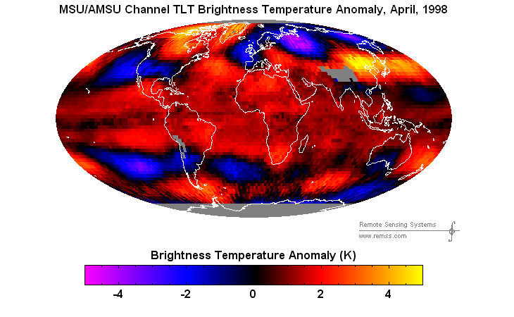
3. year: This indicates the warmest year on record so far for that particular data set. Note that the satellite data sets have 1998 as the warmest year and the others have 2014 as the warmest year.
4. ano: This is the average of the monthly anomalies of the warmest year just above.
5. mon: This is the month where that particular data set showed the highest anomaly. The months are identified by the first three letters of the month and the last two numbers of the year.
6. ano: This is the anomaly of the month just above.
7. y/m: This is the longest period of time where the slope is not positive given in years/months. So 16/2 means that for 16 years and 2 months the slope is essentially 0. Periods of around a year or less are not counted and are shown as “0”.
8. sig: This the first month for which warming is not statistically significant according to Nick’s criteria. The first three letters of the month are followed by the last two numbers of the year.
9. sy/m: This is the years and months for row 8. Depending on when the update was last done, the months may be off by one month.
10. McK: These are Dr. Ross McKitrick’s number of years for three of the data sets.
11. Jan: This is the January 2015 anomaly for that particular data set.
12. Feb: This is the February 2015 anomaly for that particular data set, etc.
14. ave: This is the average anomaly of all months to date taken by adding all numbers and dividing by the number of months.
15. rnk: This is the rank that each particular data set would have for 2015 without regards to error bars and assuming no changes. Think of it as an update 15 minutes into a game.
| Source | UAH | RSS | Had4 | Sst3 | GISS |
|---|---|---|---|---|---|
| 1.14ra | 3rd | 6th | 1st | 1st | 1st |
| 2.14a | 0.27 | 0.255 | 0.564 | 0.479 | 0.67 |
| 3.year | 1998 | 1998 | 2014 | 2014 | 2014 |
| 4.ano | 0.42 | 0.55 | 0.564 | 0.479 | 0.67 |
| 5.mon | Apr98 | Apr98 | Jan07 | Aug14 | Jan07 |
| 6.ano | 0.663 | 0.857 | 0.835 | 0.644 | 0.93 |
| 7.y/m | 6/0 | 18/4 | 0 | 0 | 0 |
| 8.sig | Aug96 | Jan93 | Apr00 | May95 | Nov00 |
| 9.sy/m | 18/8 | 22/3 | 14/11 | 19/11 | 14/5 |
| 10.McK | 16 | 26 | 19 | ||
| Source | UAH | RSS | Had4 | Sst3 | GISS |
| 11.Jan | 0.351 | 0.366 | 0.690 | 0.440 | 0.75 |
| 12.Feb | 0.296 | 0.327 | 0.656 | 0.406 | 0.78 |
| 13.Mar | 0.256 | 0.255 | 0.683 | 0.427 | 0.84 |
| Source | UAH | RSS | Had4 | Sst3 | GISS |
| 14.ave | 0.301 | 0.316 | 0.676 | 0.424 | 0.79 |
| 15.rnk | 3rd | 5th | 1st | 2nd | 1st |
If you wish to verify all of the latest anomalies, go to the following:
For UAH, version 5.6 was used. Note that WFT uses version 5.5 however this version was last updated for December 2014 and it looks like it will no longer be given.
http://vortex.nsstc.uah.edu/public/msu/t2lt/tltglhmam_5.6.txt
For RSS, see: ftp://ftp.ssmi.com/msu/monthly_time_series/rss_monthly_msu_amsu_channel_tlt_anomalies_land_and_ocean_v03_3.txt
For Hadcrut4, see: http://www.metoffice.gov.uk/hadobs/hadcrut4/data/current/time_series/HadCRUT.4.3.0.0.monthly_ns_avg.txt
For Hadsst3, see: http://www.cru.uea.ac.uk/cru/data/temperature/HadSST3-gl.dat
For GISS, see:
http://data.giss.nasa.gov/gistemp/tabledata_v3/GLB.Ts+dSST.txt
To see all points since January 2014 in the form of a graph, see the WFT graph below. Note that Hadcrut4 is the old version that has been discontinued. WFT does not show Hadcrut4.3 yet. As well, only UAH version 5.5 is shown which stopped in December. WFT does not show version 5.6 yet.
 - 1979 to Present")
As you can see, all lines have been offset so they all start at the same place in January 2014. This makes it easy to compare January 2014 with the latest anomaly.
Appendix
In this part, we are summarizing data for each set separately.
RSS
The slope is flat since December, 1996 or 18 years, 4 months. (goes to March)
For RSS: There is no statistically significant warming since January 1993: Cl from -0.014 to 1.700.
The RSS average anomaly so far for 2015 is 0.316. This would rank it as 5th place. 1998 was the warmest at 0.55. The highest ever monthly anomaly was in April of 1998 when it reached 0.857. The anomaly in 2014 was 0.255 and it was ranked 6th.
UAH
The slope is flat since April 2009 or an even 6 years. (goes to March using version 5.6)
For UAH: There is no statistically significant warming since August 1996: Cl from -0.027 to 2.198. (This is using version 5.6 according to Nick’s program.)
The UAH average anomaly so far for 2015 is 0.301. This would rank it as 3rd place. 1998 was the warmest at 0.42. The highest ever monthly anomaly was in April of 1998 when it reached 0.663. The anomaly in 2014 was 0.27 and it was ranked 3rd.
Hadcrut4.3
The slope is not flat for any period that is worth mentioning.
For Hadcrut4: There is no statistically significant warming since April 2000: Cl from -0.014 to 1.366.
The Hadcrut4 average anomaly so far for 2015 is 0.676. This would set a new record if it stayed this way. The highest ever monthly anomaly was in January of 2007 when it reached 0.835. The anomaly in 2014 was 0.564 and this set a new record.
Hadsst3
For Hadsst3, the slope is not flat for any period that is worth mentioning. For Hadsst3: There is no statistically significant warming since May 1995: Cl from -0.003 to 1.687.
The Hadsst3 average anomaly so far for 2015 is 0.424. This would rank 2nd if it stayed this way. The highest ever monthly anomaly was in August of 2014 when it reached 0.644. The anomaly in 2014 was 0.479 and this set a new record.
GISS
The slope is not flat for any period that is worth mentioning.
For GISS: There is no statistically significant warming since November 2000: Cl from -0.041 to 1.354.
The GISS average anomaly so far for 2015 is 0.79. This would set a new record if it stayed this way. The highest ever monthly anomaly was in January of 2007 when it reached 0.93. The anomaly in 2014 was 0.67 and it set a new record.
Conclusion
Nature has many negative feedbacks that help prevent Earth from getting too hot or too cold. If this were not the case, then we would not be here to discuss this. James Hansen once spoke of boiling oceans, be impressed…
UAH Update:
Version 5.6 had 2014 as third warmest and after 3 months in 2015, 5.6 was on track to be 3rd warmest.
However version 6 now has 2014 to be 6th warmest and after 3 months, version 6 is on track for 2015
to be 5th warmest, exactly like RSS.
In addition, the length of the pause on version 6 is over 18 years, similar to that of RSS.
Of course, the time for statistically significant warming would also greatly increase. I do not yet have that
period, however I expect it to be over 22 years in line with RSS.
April Update for UAH and RSS:
The April anomaly is out for UAH version 6.0 and it is 0.065, a drop of about 0.07 from March. As a result, after 4 months, UAH would rank in 8th place if the new average were to hold for the rest of the year. As well, since the pause was 18 years and 3 months after March, and since the March value was on the zero line, the pause with April is now at least 18 years and 4 months on UAH.
RSS for April is also out. It dropped from 0.255 to 0.174. Since the zero line was 0.24, the new pause will be at least 18 years and 5 months. However it could be longer. I will know for sure in 6 hours when WFT does the update. If the new average of 0.281 holds, RSS would end up in 6th place for 2015.
Up to this point, the lower troposphere does not seem to be aware of the fact that we have had an El Nino since October. See:
http://www.cpc.noaa.gov/products/analysis_monitoring/ensostuff/ensoyears.shtml
However GISS and Hadcrut4.3 are solidly in first place after 3 months by about 0.12 so it would take a huge drop in April to knock either one out of first place in April.
With respect to statistically significant warming, that is obviously going to increase greatly.
With version 5.6, Dr. McKitrick had it at 16 years while Nick Stokes had it at 18 years and 8 months.
For RSS, Dr. McKitrick had it at 26 years while Nick Stokes had it at 22 years and 3 months.
But with the pause being 18 years and 4 months on version 6, I would say Nick’s time would increase by 4 years to over 22 years.
As for Dr. McKitrick, notice that most of the points for RSS since last April when he made his calculation for RSS are below the trend line. So if he were to calculate RSS today, he could get 27 years. I have no clue about UAH6, but I would not be surprised if it would be similar.
http://www.woodfortrees.org/plot/rss/from:1988/plot/rss/from:1988/trend
Thanks Werner..
The whole discussion is nonsense, “Le Châtelier’s principle applies the species in a closed chemical equilibrium system, not the Earths climate. Its about as silly as applying Relativity to baking chicken pies
While it is true that this was its initial application, it can be applied to many things broadly speaking.
Werner Brozek says
“While it is true that this was its initial application, it can be applied to many things broadly speaking.”
What a load of ignorant crap, just shows the level of debate when all the science is against you and you have to make up snake oil to pretend there is some kind of debate
Unbolted says: “What a load of ignorant crap,…”
++++
Which part of a debate does this fall into? Which part of “all the science is against you” are you specifically talking about?
Please see the following near the end from another reader:
http://wattsupwiththat.com/2015/05/03/le-chatelier-and-climate-change-now-includes-march-data/#comment-1925306
Well the first reference is just pseudoscience misinformation and the second correctly states the atmospheric CO2 is part of an equilibrium system with oceanic carbonate. That is, the ocean is a carbon sink and the rate of uptake has been well documented. So what, none of this is any support for your unfounded ideas.
Do you have any Chemistry qualifications, you give the impression you are struggling with the basic concepts?
I have an engineering degree, but Lubos Motl was an assistant professor at Harvard University. And his article was the one I referenced at the start. If you do not believe me, you may want to take it up with him.
So the answer is no and Lubos Motl doesn’t either. Amateur nonsense.
“Nature has many negative feedbacks that help prevent Earth from getting too hot or too cold. If this were not the case, then we would not be here to discuss this.”
This may be the most astute sentence published here (or anywhere) on climate that I have seen in a long, long time.
We have a very complex weather system on this planet and mankind is only beginning to learn how it operates in regards to all the feedbacks. One thing we know, over time the climate has been remarkably stable.
False Precision Fallacy
==================
One really shouldn’t give any weight to a difference of 100th or even 1000th of a degree. This field of
studycharlatanism is rife with the false precision fallacy.What is the average temp of five measurements of 51F, 53F, 58F, 63F and 61F? 57.2F. But we were only given temperature values accurate to +/- half a degree. Clearly there was no measurement accurate to +/- 0.1 degrees. However, taking the average and leaving the digits gives a false sense of precision.
To be honest, the average should be given as 57F, within the accuracy of the original measurements. Do this and all the recent global warming disappears.
Fair enough. But that does not change the fact that UAH is 8th warmest after 4 months, or whatever range your error bars would indicate, and GISS is well on the way to a new record.
Ranking warmest numerically can easily present an inaccurate view. For instance, ten men run a race. First place comes in first by .75 seconds, while 2nd through 10th place have a total spread of ONLY .33 seconds.

Second lace is much closer to last in this example then to first.
Such is the case in comparing RSS and UAH to the surface record. Allow me to paint a pretty picture.
Werner, regarding the above post, lease note that NOAA claimed what?, a 36% chance of 2014 being number one based on .03 degree record. Using the same statistical method, then NOAA would say with 100 percent certainty that 1998 was hotter then 2014 and, thus far, 2015.
I do not have the NOAA numbers handy, but my understanding is that if the anomaly difference is 0.1 compared to the next warmest year, then you are close to 100%. And after 3 months, both GISS and Hadcrut4.3 are above this, so they could set a record with “100%” confidence, or close to it. But there are 9 months to go so anything can happen.
No it should not. One can calculate the propagation of uncertainties. Taking the mean of 5 values each with an uncertainty of 0.5 degrees leaves an uncertainty for the mean of about 0.2 degrees. Increasing the number of measurements further decreases the uncertainty. It’s just statistics.
“Taking the mean of 5 values each with an uncertainty of 0.5 degrees leaves an uncertainty for the mean of about 0.2 degrees. ”
I do not think this is correct.
What you say here is not at all what my understanding is.
For one thing, it is unstated if the five values are different measurement of the same measurand, or not. In other words, are these five readings from the same place and time, or from five different days or locations?
Then one must also define the systemic errors and the random errors, and calculate for each. The nature of what is being averaged must then be taken into account.
There is no reason to suppose that five readings on different days (or locations) will have a standard distribution!
I the given example, every one of the stated values might be .49 degrees higher than the true temp, or a similar amount too low. The reported numbers would remain the same in either case, but the trueness .98 apart.
And one must define terms.
Although I am loath to quote Wikipedia, for a subject such as this it serves as a convenient reference, and what is written her jibes with how I was taught:
“Accuracy and precision are defined in terms of systematic and random errors. The more common definition associates accuracy with systematic errors and precision with random errors. Another definition, advanced by ISO, associates trueness with systematic errors and precision with random errors, and defines accuracy as the combination of both trueness and precision.”
“In the fields of science, engineering, industry, and statistics, the accuracy of a measurement system is the degree of closeness of measurements of a quantity to that quantity’s true value.[1] The precision of a measurement system, related to reproducibility and repeatability, is the degree to which repeated measurements under unchanged conditions show the same results.[1][2] Although the two words precision and accuracy can be synonymous in colloquial use, they are deliberately contrasted in the context of the scientific method.
A measurement system can be accurate but not precise, precise but not accurate, neither, or both. For example, if an experiment contains a systematic error, then increasing the sample size generally increases precision but does not improve accuracy. The result would be a consistent yet inaccurate string of results from the flawed experiment. Eliminating the systematic error improves accuracy but does not change precision.
A measurement system is considered valid if it is both accurate and precise. Related terms include bias (non-random or directed effects caused by a factor or factors unrelated to the independent variable) and error (random variability).
The terminology is also applied to indirect measurements—that is, values obtained by a computational procedure from observed data.
In addition to accuracy and precision, measurements may also have a measurement resolution, which is the smallest change in the underlying physical quantity that produces a response in the measurement.
In numerical analysis, accuracy is also the nearness of a calculation to the true value; while precision is the resolution of the representation, typically defined by the number of decimal or binary digits.
Statistical literature prefers to use the terms bias and variability instead of accuracy and precision. Bias is the amount of inaccuracy and variability is the amount of imprecision”
http://en.wikipedia.org/wiki/Accuracy_and_precision
Aran, perhaps you could explain why you believe that more measurements means that uncertainty decreases?
If this is true, then presumably when one has thousands of readings from all over the world for every day of the year, there would no longer be any uncertainty to speak of, such being vanishingly small by then. Even if all the thermometers had large random errors and systemic ones!
I am not a mathematician, but it seems highly illogical to think that having a bunch of readings makes each one more “true”.
numbers with errors-
http://www.math-mate.com/chapter34_4.shtml
Exactly.
Unless the errors are NOT randomly distributed about the mean that is the case.
In the case of thermometer calibration it would be expected that they were random, unless a partucular thermometer type was always used that had been calibrated to a wrong standard. Or a particular measurement technique that always meant over reading were the case.
But even then the delta – the change in average – would still be valid. As long as the same thermometer were used in the same way every time. In the same environment. And the thermometer didn’t change with age…
In the given example, it was not stated that these were five measurements of the same measurand.
In fact, since the focus of our discussions here are always regarding some aspect of climate, and temperature readings are generally only taken once in each location using one device, the averages that we are constantly yammering about are from different sites, and different days, all averaged together.
This is completely different than the case where one is attempting to derive a precise and accurate number by averaging numerous readings at the same place and the same time of the same quantity.
In the latter case, standard distributions might be assumed, and many readings will tend to lower the random errors inherent in any measurements.
The same can not be said for temperature values from different points on the globe. Each reading is independent, and errors can not be assumed to cancel or diminish. Averaging cannot add a decimal place of precision.
Is there anywhere that the temperature is taken by having five thermometers and five readings for each each day? I think not, so to argue as if that is what is being discussed makes no sense to me.
*crickets*
Robert, back in the Early Cretaceous when I was a Chem. E. student, a prof asked us during a class to calculate a result, using temp data measured to the tenth of a degree.
When a student volunteered an answer to the thousandth degree he had worked out on his trusty K & E (old folks will understand the reference), the prof smiled and said, “That’s quite a slide rule you got there, son!”
Heh.
I’m a bit surprised that a real professor would use that insulting term of address, “son”.
Even though I have taught in three American universities, i have never heard it used.
“I’m a bit surprised that a real professor would use that insulting term of address.”
Perhaps not so insulting in certain places and depending on the tone of the lectures. Some are very formal, and some much less so.
In the south, this is a commonly used term in informal speech, although it seems to becoming less so.
And maybe he was just calling him that because he was a very bright young man.
RoHa, the term ‘son’ isn’t insulting! Jeez! Everyone is so ready to take offence. What has happened to people? People seem to want a go and cry in the corner as soon as someone ‘disrespects’ them. I’ve been called ‘son’ thousands of times – and not by my dad. I’ve been called all sorts of names, too, but none of them bother me. Why should they – it’s if you hit me that it matters!
Your professor was Foghorn Leghorn?
“Your professor was Foghorn Leghorn?”
Now cut that out boy, or I’ll spank you where the feathers are thinnest.
Robert of Ottawa,
Your measurements I presume are made on a single device for a specific time period:
N = 5 measurements, each with only two significant digits reported, not: “accurate to +/- half a degree.”
Average = 57 F, Not “57.2 F” – (remember only 2 significant digits)
range (R) : (X max – X min) = 12 F,
Uncertainty of the mean: R / (2 * square root N) = +/- 2.7 F ,
Average temp of 5 measurements, i.e the reported value = 57 +/- 2.7 F for the specific time period.
The average of five readings which are each accurate to the nearest degree (i,e, are +- 0.5 degree out worst case) is statistically accurate to that error margin divided by the sample size, so 57.2°F +- 0.1°F.
IF of course, there is no consistent bias in the readings. And they have a normal distribution about the mean.
Many years ago in skool, we did some experiments to determine the gravitational constant, and the most accurate way was by timing pendulums.
Every member of the class did this, and the results ranged quite widely. However the average of the results when one outlier was removed, were within 0.5% of the generally accepted value.
If you dont believe me, do a Monte Carlo analysis on the average of a fixed number to which a random offset is added. You will find it very near the constant. In the same way that throwing a coin many times will result in a very close to 50% heads over throws result.
I see this claim very often in sceptic blogs, that an average can be no more exact than the accuracy of any one of the sample points. This is simply not true, and degrades the sceptic position.
” In the same environment. And the thermometer didn’t change with age…”
this is what the error margins are for. there are many more things that can change between the same model of thermometer and siting. how on earth can one claim that the average of a particular thermometer be without bias etc when the claim is already accepted that the thermometer has an error margin of +-x. calibrate within its error margin and hope it never changes…
You are correct that an average can easily be more accurate than a single sample point, and I too am driven to distraction by those who claim otherwise. However, I am equally appalled by those who assume error bars consistent with a model of independent errors when there are obvious long term correlations in the data.
That’s not true….based on how I read this.
You don’t have a standard or constant like gravity. You don’t know what the actual temp is and you use measuring devices to see what they say. Measuring devices that have error built into them due to manufacturing and component limitations and tolerances.
If I tell you that the equipment with which you are measuring temp is only accurate to within +/- .5 degrees, millions of measurements do not make the equipment more accurate. It’s still and always +/- .5 degrees. In fact it could always bias 1 way and you may not know it. You calibrate it as close as you can and go from there.
You got it right HFB.
And we are never talking about the same temperature in the same place measured numerous times. We are talking about climate change, which uses readings from all over the world averaged together. Which makes it even worse. Not better.
Robert, If the five values you give are all the information that will ever be collected for your hypothetical observation site you can readily calculate all that can be logically deduced about its long-term state, provided that you assume that the observations you quote are a sample from a normally distributed population and are independent.. These assumptions are widely made, and in many cases reasonably valid, though one never actually knows!
Here’s the nitty gritty:- Mean 57.200, Std Dev 5.11859, Std Error 2.2891, Skewness -0.1928, Kurtosis -0.23014, Jarque Bera statistic 1.134 (Critical value for 95% 1.423), Approx prob for such a value 0.567 (needs to below 0.05 to disprove normality by the usual standard), 95% confidence intervals for a further single observation 42.986 to 71.414, and for the long-term mean 50.843 and 63.557.
For comparison I’ve generated a pseudo-normal variable of 100 items, where I specified a mean near 57.2 and an SD of 5. It produced the following:- Mean 57.103, SD 5.005, 95% lower confidence intervals 47.17, 56.11, and upper 58.096, 67.03, Jarue Bera 0.772 with a prob of 0.68. Thus very “normal” as expected, with much narrower intervals for the long-term mean. It all goes to show that you need to be careful about guessing averages from small amounts of data.
I’m being deliberately pedantic here of course. It is simply to illustrate that the amount of information you supplied really isn’t sufficient to do much in the way guessing what the “real” value is. Your statement on the mean value of the observations is totally correct, as are your comments of how it should be interpreted, but as you can see, to say much more in a statistical context is not very useful. These are simply the facts of life regarding analysis of observations, but in my experience not many people seem to know much about them.
Your estimate of 57.2 as the mean is the best that can be done, but as you say, don’t read too much into it!
Standard data handling methods govern presentation of significant figures.
Depending on the uncertainties, the number of significant figures is selected.
As I was taught, averages can rightly be quoted to a extra decimal place to the original data.
So thenths in the above case look OK, showing hundredths of a degree is stretching it.
“And in the end, the temperature will not be as hot as you may expect due to the counteraction.”
Actually, it will be exactly 20 degrees celsius. You might look at the definition of temperature, or alternatively the 0th law of thermodynamics.
What I wanted to say is, why should I read the rest of this post if you don’t understand thermal equilibrium better known as temperature?
Ooops! You got me there! I should have put a time limit on it such as five minutes. Sorry about that!
“In this case, it does so by freezing the water until it is all gone. And only after this will the temperature go down. And in the end, the temperature will not be as cold as you may expect due to the counteraction.”
Max, I picked up the same point on my way through the article. I would not have said that there has to be a time element, but would have constrained it with a total energy limit. The heat will be transferred from the hotter or colder environment at some rate (Joules per second) or up to some total. So for ANY given total time or total energy (regardless of time) the conclusion holds true.
Because this is a pretty basic omission it would be good to add a sentence saying at least that it holds true for a given time period – not to leave it as is.
Because alarmism thrives on confusing energy with temperature it is a great protection for the public to have a basic understanding of thermodynamics. It is not very complicated and is best taught by constantly referring to the units. Some units are ‘intensive’ like temperature with one dimension. Some are ‘extensive’ with two or three dimensions. The fuddle-duddle math of climate alarm has roots in the hope that the public doesn’t know how to think about the subject. The solution is education. An educated public is far less likely to attracted by toxic ideologies.
Sorry Max, you are the one who cannot understand simple concepts. The ice and water will actually cool the room to less than 20 degrees. It is a shame you must close your mind to new concepts.
It all depends on what assumptions we are making and I did not elaborate on this point. For example, how large is the room? Is it large enough to make the drop from 20.0000 to 19.9999 negligible for example? Is there a heat source that keeps the room at a steady 20 C, regardless what else happens? Is the room perfectly insulated? Are we waiting long enough for equilibrium to be reached? Etc.
Well, then we end up with the same problem about the definition of global temperature, as it is not temperature but just some value that gives a hint about temperature development.
That is a valid but totally different issue. Ignoring humidity, the global temperature varies by 3.8 C between January and June. But if we take into consideration whether very humid +40 C air is warmer or whether -30 C dry air is warmer makes a huge difference.
Dan the cup, water and ice were constrained. The room was not. Your poke is a miss.
The ocean and atmosphere climate system does not “count” as a system at equilibrium because there is always a net flow of energy from the sun and then radiating out into space. Hence the LeCh. principle in this simple form does not apply. Remember, life cannot exist in a system at thermodynamic equilibrium. Life flourishes on earth — hence earth is far from thermodynamic equilibrium
While it is true that Earth is never in equilibrium, it is also true that Earth is always striving to reach equilibrium.
@Brozek
Thank you
No it isn’t, unless you believe in divine intervention, the Gaia Hypothesis, or similar bollocks.
Yes it is, and the deity’s name is Entropy.
@D.Cohen
“…life cannot exist in a system at thermodynamic equilibrium. Life flourishes on earth — hence earth is far from thermodynamic equilibrium”
So, increasing the solar constant won’t lead to higher temperatures on earth`? Oh, I did not refer to the sentence cited by me, but this one is so wrong, it’s not even false.
Its a bounded system and no matter how many games you play with it the atmospheric “green house gasses” are not the control knob. Energy input from the sun, angle of the earth in relation to the sun, mass of the ocean, albedo, cloud cover and the mass of the atmosphere are the critical factors. Equilibrium is the range of temperatures possible in this bounded system so in essence the system is always in equilibrium, only a change in one of these controlling factors will move the range of possible temperatures and a new state of equilibrium will be met. The possible temperature range when modifying the actual control knobs is somewhere between slightly above absolute zero and the temperature that it would take to vaporize the earth, the few tenths of a degree K change we see and discuss is noise in the system.
When I see the three identical rates of temperature rises in the last century and a half, and with only the last being with rising CO2, and I see the nearly identical slopes of pause after those three rises, it occurs to me that either CO2 sensitivity is pretty small, or something powerful is pushing against the CO2 radiative effect.
Since it seems the oceanic oscillations account for the oscillations around the gradual rising trend, then this powerful agent is not the oceans. What else could it be but the sun? Well, it could be that the CO2 effect is weak.
Take your choice. Which would you prefer?
Which is more likely? I dunno, but I have my suspicions.
=======================
It’s a fairly stark choice: Either the CO2 effect is small, or the sun(or something) is pushing the Earth in a cooling direction.
=======================
At the moment, at least on the satellite data sets, it seems as if the spotless sun is “stronger” than both high CO2 levels as well as an El Nino combined. However we will see if this changes over the next few months.
Boiling oceans may sound like lunacy but I’ve actually had dim witted alarmists tell me such. I hadn’t appreciated the source of their claims.
If all the energy received by the oceans from the sun went into boiling the oceans and none was lost to anything else, at all, it would take 720 years to boil them.
Real losses ensure this can never happen, even if the sun’s energy output doubled. The suggestion that AG CO2 can cause the oceans to boil doesn’t make it out of the ditch of ‘stupidity’ onto the shore of ‘wrong’.
Yes, Hansen told us that the total influence for a doubling of CO2 was 3.7W and that the amount of that not taken up (for the CO2 rise relative to preindustrial) by the biosphere is 0.6W per square meter. A single incandescent Christmas light is about 1W and can act as a proxy. So if we laid a mat of little christmas lights 1 per square meter 1 meter above the ocean, leaving that ocean to cool naturally through evaporation how long would it take to get to boiling point.
Try it yourself, take a 1 Watt torch and suspend it, shining into a bucket of water, put another bucket of water next to it with an equal quantity of water (weigh the water), and leave both in the sun. when the bucket is down to 1/4 full measure the temperature of the two buckets. leave the buckets until they completely evaporate, when one evaporates weigh the amount of water in the other bucket. Does the bucket with the torch shining in ever boil?
Now in theory the bucket with the torch should be hotter, but it will not, the evaporation in the torch lit bucket will rise slightly so that the surface temperature of the water is affected less. Now at the same time both buckets are being flooded by variable effects, wind, rain, sun/cloud. the thermal conducivity of the earth under the bucket (depending on its wetness). If you do this 1000 times the chances are the outcomes will be completely random, despite the input of a constant watt of power to one of the buckets. (Now this is a watt into about 100 square cm extrapolate this to the same torch shining into an ocean square meter, x maybe 1Km depth (A cubic kiliometer (1000 Tonnes) of water).
Another experiment – take an large open saucepan of water, put it on the stove and put the heating element on 1. In this case you are pouring maybe 200 watts into maybe just 50 square cm (surface area) of water free to interact with the environment- will the water EVER boil? – No, the termperature just rises, until the losses equal the power input.
In the earth’s case, the sun is constantly pouring a Kiliiowatt into the ocean (well 300 or so watts averaged), and the ocean manages to only get to a few degrees above freezing before equilibriating (4.5 deg C average), Then we add a christmas light of energy to it (an extra 0.2%) and suddenly the oceans will come to a boil?
This is how ridiculous this is, no amount of low grade energy like this can boil the oceans
This myth is so BUSTED, it’s beyond stupid!
Boiling oceans sounds like lunacy because it is.
The notion that the oceans of the earth could possibly boil from a few degrees of temperature rise is beyond ludicrous, it is beyond idiotic, it is beyond alarmist hype.
It is literally insanity for anyone to believe that it could be true.
I would be interested to read somebody’s calculation of what would happen to thunderstorm activity if the oceans would even get to 100 or 110 or 120 degrees Fahrenheit?
I understand Hansen later retracted that statement. But to make such an alarmist statement in the first place is something. And as Tony pointed out above, others repeat that point without realizing how impossible it is.
Very good point Mr. Brozek.
I am reminded of a talk given by Dr. Lindzen, in which he was discussing a similar sort of thing. He had been listening to a speech by the President of MIT, in which she said that climate change was accelerating. When he approached her to ask why she was saying this, she said had it on good authority that this was the position of the IPCC. It was not true that the IPCC said this, but by now, everyone can say that the President of MIT says CC is accelerating.
Thank you! I will listen to it tomorrow.
All I now is that this decade will be the warmest, or the second warmest, this Century. Make sure this is understood in Paris 2015.
Why?
LOL Stein Gral even capitalized “century” for emphasis! Since there are only two decades to “this Century” so far, then this decade can only be the warmest (second coolest) or the second warmest (coolest).
“Since there are only two decades to “this Century” ”
I bump into that a lot. So Stein is technically correct in fact, but that fact is often irrelevant when put into perspective.
Like the alarmist’s claim of Antarctica losing “city sized” chunks of ice. A fact, but so what? The yearly summer – winter ice extent delta is more than the entire area of the CONUS.
This decade will be either the first or second warmest of this new century. I am absolutely sure that you are absolutely correct. To me it seems to be a mathematical certainty. It is seldom in climate science that we can make a statement about the future which is absolutely true.
Cheers.
Since this century is only 15 years old, is it not also true that this decade is the coolest or second coolest this century? ☺
Of course ! (I was just having fun, but seems like some did not take it, even WUWT-readers … ?)
Reminds me of an old British joke: A journalist says to John Lennon, “Is Ringo Starr the best drummer in the world?” Lennon says, “He isn’t even the best drummer in the Beatles!”
Should that be “Best” drummer (as in Pete?)
This reminds me of an old joke from the Cold War days.
The U.S. And the U.S.S.R. met in a two-country athletic contest to determine who had the fastest athletes. The next day, the U.S. headlines were, “U.S. Beats U.S.S.R. In Track Meet.” The headlines in the U.S.S.R. we’re, “U.S.S.R. Places Second in International Competition. U.S. Finishes Next to Last.”
“Lies, damn lies, and climate science.”
Props to Max Photon.
Re 2014 being the ‘warmest’ year: is 14.6C (or whatever it was) ‘warm’ ??
At least the ghastly ‘hottest’ seems to be going out of favour.
And wasn’t it the case that the margin of error was 5 times greater than
the difference between 2014 and the nearest ‘competitor’ ?
Further, the errors margins quoted are the statistical errors, which may
be somewhat less than the overall survey error. This is a common failing
among those reporting on consumer research and polling. How often have
you heard the perpetrators claim that, having done1000 interviews, the results
of their survey are subject to an error of +- 3.4% (or whatever it might be) ?
Bilgewater. The survey error is +- 5 – 7% … the 3.4 figure depends on the
methodology/sampling complying with a number of stringent criteria, which
compliance never happens, or very rarely.
And so it is with the networks of temperature stations, which some might
describe as a ‘survey’. More like a dog’s breakfast if you ask me.
That is correct. See my earlier post here where I discuss this: http://wattsupwiththat.com/2015/02/03/only-satellites-show-pause-wuwt-now-includes-december-data/
As well, note that this only applies to GISS and Hadcrut4.3. The satellites still have 1998 as the warmest year.
i know the outcome already: GIss will make it a record year.
problem is i don’t believe the GISS dataset anymore
Hadcrut4.3 is the same as GISS so far. So which are the outliers? Is it GISS and Hadcrut4.3 or is it RSS and UAH?
I suspect you pays your money and you takes your choice.
One must take the good with some bads.
======
Oh, they are getting away with the goods, that much is for sure, eh Kim?
HADCRUT4 and GISS don’t look the same to me.
What you are seeing is Hadcrut4.2 which has not been updated since July 2014 but this is all that WFT shows.
At the time, Hadcrut4.2 was flat since February 2001 or 13 years, 6 months. (went to July).
Hadcrut4.3 replaced Hadcrut4.2 and went on to set a record in 2014. Furthermore, it is set to have a new record in 2015. Both of these last two facts apply to GISS.
I wonder if 4.3 still shows the NH with a decided downturn…
I have no clue. It would be nice if WFT were updated. I know of two people who have written to Paul about this but without success.
Data tampering and the Internet not forgetting.
What would it have been if they were still using the semi-adjusted HADCRUT3 version instead of the full-adjusted HADCRUT4.
12 month
average
anomaly HADCRUT3 HADCRUT4
Dec 1998 0.55 0.52
Dec 2011 0.34 0.40
Increase/ -0.21 -0.12
The new version increases warming (or rather decreases cooling) since 1998 by 0.09C, a significant amount for a 13 year time span. Whilst the changes should not affect the trend in future years, they will affect the debate as to whether temperatures have increased in the last decade or so.
https://notalotofpeopleknowthat.wordpress.com/2012/10/10/hadcrut4-v-hadcrut3/Decrease
Also –
100% Of Reported US Warming Since 1990 Is Fake
Posted on February 4, 2015 by stevengoddard
https://stevengoddard.wordpress.com/2015/02/04/100-of-reported-us-warming-since-1990-is-fake/
The animation below flashes between the average of measured adjusted USHCN temperatures, and the estimated (infilled) ones – which are marked with an “E”. As you can see, all US warming since 1990 is due to infilling fake data. And even the measured zero warming temperatures have been tampered with using various other adjustments. USHCN is losing data at a spectacular rate over the last three years, with more than 50% of the 2015 data marked as estimated, and nearly 40% of the 2014 data marked as estimated.
And last – (1) The Climate of 1997 – Annual Global Temperature Index = 16.92°C.
http://www.ncdc.noaa.gov/sotc/global/1997/13
(2) 2014 annual global land and ocean surfaces temperature = 0.69°C above 13.9°C = 14.59°C
http://www.ncdc.noaa.gov/sotc/global/2014/13
Which number do you think NCDC/NOAA thinks is the record high. Failure at 3rd grade math or failure to scrub all the past. (See the ‘Ministry of Truth’ 1984).
How much of the Hadcrut4 increase is real?
http://www.woodfortrees.org/plot/hadcrut3gl/from:1997.3/to:2012.9/offset:0.043/plot/hadcrut3gl/from:1997.3/to:2012.9/trend/detrend/plot/hadcrut4gl/from:1997.3/to/plot/hadcrut4gl/from:1997.3/to:2012.9/trend/detrend:-0.0145/plot/hadcrut4gl/from:1997.3/trend/detrend:-0.0317
..” And only after this will the temperature go down. And in the end, the temperature will not be as cold as you may expect due to the counteraction.”
This whole thing is fairly rediculuse . The above quote is simply referring to latent heat and has nothing to do with “trying to counteract” or contains anything unexpected.
If you change a parameter in a system in equalibrium, a new equalibrium will be reached to balance the intputs and outputs. There is nothing “anticipating” the change and adjusting accordingly to balance it.
The main issue with climate prediction is that nobody knows ALL the inputs, outputs and feedback loops that control it. Looking at billions of years of proxy records it seems to indicate the climate is stuck within a narrow band of temperature for “whatever reason” or mechanism.
This is a good thread to pose this:
As the concentration of CO2 rises from 350 to 450, what is the power absorption is watts per square meter that goes into additional biomass in the ocean and on land?
The 30% of improvement in food production being attributed to CO2 fertilisation – that takes more energy out of the incident light ‘darkening’ the surface, meaning there isn’t as much energy to send away from the Earth. How much exactly? Approximately?
If there is established a new equilibrium, it will include the absorption of energy in endothermic conversion of CO2 into biomass. How many watts?
Good and interesting thoughts ! Perhaps this is “taking away energy” so it will not be warmer, but colder ? – since the overall energy ballance is constant ? Or am I lost here ?
However when all of this extra food is eaten by humans or animals, then the heat is given back as metabolism occurs, is it not? I think we need a biologist to take this further.
Photosythesis by my calcs absorbs about 3-4 Watts per square meter so 10% increase represents 0.3W about 1/2 the 0.6W supposed imbalance, and no Werner that is not true. When it is eaten, some of the energy is absorbed and some is excreted, energy leaves the animal as:
Sensible heat (from body temperature), kinetic, chemical, sound and electrical energies.
a fraction of the carbon is returned as CO2 to feed the plants again.
Some carbon gets retained. For every Killogram of carbon retained about 3.5kg of CO2 is sequestered.
There is a myth going around that the breakdown of plants results in the same amount of CO2 being released later – that is bulldust – as clearly evidenced by the amount of Oxygen in the atmosphere, pretty much all of it come from decomposing CO2 to solid/liquid Carbon compounds and O2.
Earth is on a one way trip to a Nitrogen/Oxygen atmosphere and isn’t heading back to a CO2 atmosphere any time soon. In fact if it weren’t for us, the atmosphere would be approaching CO2 depletion and the end of all life.
I don’t think we have any idea how much biomass, and hence carbon, is settling to the bottom of the ocean, practically irreversibly sequestered.
================
I believe we would still have some life, certain types of bacteria and the colonies around hydrothermal vents…the so called black smokers would be around for a while.
Plus, bolides impacting limestone or other carbonate rock formations might occasionally release a large amount of CO2, no?
As well as volcanoes, particularly following subduction of carbonate bearing sedimentary rocks.
While we are at it, what is the energy content of the ocean compost at the bottom of the oceans?
How are you measuring power? How are you measuring “warmer”/”colder”? If you are trying to use air temperature to measure energy, your answer will be garbage as temperature is not a measurement of energy, and as the author of the article points out, energy and temperature do not necessarily even correlate. I’m still trying to figure out how el-nino/nina can “change” the average global temperature, but weather/wind i.e. natural fluctuations can be ruled out as the cause of global “warming”. If the “heat” can go into the oceans, then the “heat” can come out of the oceans. The short of it is temperature alone is a useless measurement of the amount of energy the earth is retaining.
“Then the oceans would heat up more and water would evaporate more causing more clouds and perhaps earlier clouds which would reflect more heat away. As a result, the earth still warms but slower than would otherwise be the case.” This comment neglects the energy needed to convert said water into vapor. Suppose a change in wind currents drive this high humidity air over the Sahara where it is promptly absorbed by the sand/plants, now the humidity drops also so less clouds? It is a chaotic system w/too many variables, and we try to measure it by using temperature as a measurement of energy, epic fail. Yes, I know the ideal gas law and if it applied then the earths average temperature would be linearly rising if CAGW was true. You can’t change the energy of a system by moving it from one place to another and earths temperature varies from year to year and month to month. In the desert example, the humidity coming out of the air changes the pressure and number of moles which changes the temperature, and since average global temperatures don’t account for humidity or air pressure you can’t use temperature as a measure if you are really talking about energy.
So, no you are not lost, just realizing the amount of variables involved and the inherent inconsistency of it all.
To all the AGW believers, what are we measuring as rising when we talk about “warming”, temperature or energy? Remember if it is temperature then you can’t use “the oceans ate my warming” because that argument is about energy.
Also, has anyone calculated the increase in the circumference and atmosphere of the earths atmosphere by a rising of the temps and pressure, which increases the volume thereby modulating the pressure and the temperature? Would I be correct to presume a larger surface area would radiate more energy into space? Is it significant?
If the deep oceans warm from 3.0 C to 3.1 C, can that heat ever come out to warm the air?
True, but I did mention it earlier with the lake. Realize that I am barely scratching the surface here and a book or a doctor’s thesis could be written about Le Chatelier and climate.
Satellites in orbit could be affected by more drag, but I do not believe the area affects energy to space. But higher temperatures higher up would be more significant.
Don’t know the answer to your question Crispin but do know that global increases in plant productively and vegetative health are resulting in increasing evapotranspiration, which is having an effect,
Regionally, the Midwest Cornbelt has been like a giant laboratory over the last 3 decades. Corn plant populations have doubled during that time frame. The more tightly packed millions of acres of corn, have a big effect on weather, sometimes over an area the size of numerous states.
Starting in May(with early planting and corn off to an early start) and lasting thru August, increased transpiration from these plants causes in increase in dew points of over 5 deg C in some cases.
This causes a smaller diurnal temp range(lower highs/higher lows) lower lifting condensation levels/earlier cumulus formation, more precipitable water/rain and a positive feedback from the increase in rainfall, recharging surface moisture, which serves the corn plants and lead to additional evapotranspiration.
On a global scale, because of atmospheric fertilization from CO2, this effect is not as pronounced as the Midwest but is taking place during the growing seasons at mid/high latitudes and year round farther south.
Thanks everyone. I agree that there is a tangible change is the energy absorbed. I was wondering if the models consider that the efficiency of conversion to biomass increases with a rise in CO2 concentration. Perhaps some or all of the ‘missing heat’, which is the result of a bunch of modelling and fudge factors, is simply being absorbed. It is coal burning in reverse.
The energy available from burning a forest, net, per annum, is about 60% of the converted energy (no citation) because of the root system and tree products other than wood.
That could be used to calculate an energy conversion rate. The conversion efficiency of a maize field is high. The oceans are floating fields of microscopic plants. They too will benefit.
The globe’s biome may be more powerful than the globe’s people. It would be kinda funny if it turns out that 97% of the CO2 rise is from the oceans and the big jump is vegetative production is almost all natural. It seems we are puny after all.
Mike at 6:22 “Regionally, the Midwest Cornbelt has been like a giant laboratory over the last 3 decades.”
When I lived in the Corn belt (Iowa, actually) the crops were not irrigated. Much of the natural vegetation was grass. So, my thought is that the outcomes you suggest may be less than in some other regions.
I now live in a region where the once very dry land (under 10 inches of precip/year) is currently irrigated. Use Google Earth (or some such thing) and look for these towns in the State of Washington; then zoom-out:
Sunnyside (early, flood irrigation) [likewise Yakima and Ellensburg to the north];
The rest of these now specialize in central pivot irrigation.
Look for the green circles:
Irrigon, Oregon
Warden, WA
Quincy, WA
Picture:
http://img.bosscdn.com/photo/product/b9c2059a20f1ea14ef99873cfb272448/dyp-center-pivot-irrigation-system.jpg
I can’t.
However, it is good to remember David’s law; (-; “There are only two things that can change the energy content of any system in a rqdiative balance; a change in input, or a change in some aspect of the energy residence time within the system.”
To Werner Brozek at 4:36
Here are numbers you are looking for.
Sorry, the link did not work, so another try:
http://hyperphysics.phy-astr.gsu.edu/hbase/thermo/heatreg.html
Thank you! It looks like the human body also obeys La Chatelier’s Principle.
Le Châtelier’s principle does not really apply to your 2 examples.
If you do not know what the temperatures would be you have not applied all the facts at your disposal.
If you express surprise at where the conditions end up, ditto.
The principle though is to be applauded, CO2 increase on it’s own has a known effect on temperature in a test tube.
The multitude of feedbacks that oppose it are not known or identified and is the reason we do not have run away Climate change.
Surely we are due for some cold weather soon.
My thoughts exactly angeck2014.
If your dumb enough not to know the feed backs in place – it will always suprise you with its magical brilliance and intuition when everything works out.
Somebody needs to explain this “phenomenon” under discussion a bit better because it sounds like just another “word salad of wonder”.
I do not believe any one knows all forcings and all feedbacks. But the net result has to be that the net feedbacks are negative since we have never had run away cooling or heating. In other words, our Earth has a built in stability that allows only a limited change to its climate change.
Werner Brozek says:
…our Earth has a built in stability that allows only a limited change to its climate change.
That appears to be true. Prof Richard Lindzen writes:
There is ample evidence that the Earth’s temperature as measured at the equator has remained within ± 1°C for more than the past billion years. Those temperatures have not changed over the past century.
Natural variability increases as one approaches the Poles. But the planet’s over-all average temperature is amazingly constant, and it does not seem to matter what the atmospheric CO2 concentration is. The “carbon” narrative appears to be a red herring.
Werner Brozek
The April anomaly is out for UAH version 6.0 and it is 0.065, a drop of about 0.07 from March.
RSS for April is also out. It dropped from 0.255 to 0.174.
Will Gavin have to double down on his adjustments of the past to keep the land records up?
I will have been born in the last Ice Age at this rate, 1951.
My next post in a month will talk about the large discrepancies between the satellites and others. With the latest from Dr. Spencer, no one can claim RSS is just an outlier. Whatever Gavin does, he has to make sure it at least looks plausible. Of course that would be in the eye of the beholder.
I do not see how anything Gavin does with manipulated data will ever be plausible to any but the completely credulous.
And those folks need no convincing.
The big question is, what would it take to dissuade the average CAGW adherent?
Perhaps a huge newspaper headline saying an ice age is coming and that the scientists were wrong about global warming.
If it starts cooling, I bet that they will arrive at a way that the coming ice age was caused by warming. What will remain the same is the solution: More studies, more government control, less energy usage, more do-as-I-say-not-as-I-do sermonizing by the usual suspects, etc.
They may want to try that, but most people would see right through that. Even now, people recollect predictions about an ice age in the seventies, so they are skeptical about warming now.
The pause for RSS is now 221 months or 18 years and 5 months from December 1996 to April 2015.
Part the first: How much did anthropogenic CO2 contribute to the increase in atmospheric CO2 between 1750 and 2011?
Atmospheric dry air:……………………………5.14E18 kg
Atmospheric CO2 @ 390.5 ppm:……………….3.05E15 kg
(All ppm based on moles.)
Per IPCC AR5:
1750………………..278.0 ppm…………….2.17E15 kg
2011………………..390.5 ppm…………….3.05E15 kg
Increase……………..112.5 ppm…….………8.78E14 kg
Added anthropogenic CO2………………….5.55E14 kg
Retained in atmosphere, 45%:……………….2.50E14 kg
Added anthropogenic Fossil Fuel CO2….…..3.67E14 kg
Retained in atmosphere, 45%:……………….2.50E14 kg
Contribution of anthro CO2 to increase between 1750 and 2011: 2.50/8.78 = 28.5%.
Contribution of anthro CO2 to increase in atmospheric content: 2.50/30.5 = 8.2%.
Contribution of anthro FF CO2 to increase between 1750 and 2011: 2.50/8.78 = 19.2%.
Contribution of anthro FF CO2 to increase in atmospheric content: 2.50/30.5 = 5.5%.
The popular notion seems to be that anthropogenic CO2 was responsible for all of the added atmospheric CO2 between 1750 and 2011. The numbers don’t seem to bear that out. Over 70% might be due to natural variability, e.g ocean floor geothermal heat flux outgassing CO2 or volcanic vents producing CO2 or an entire world of unknown unknowns.
Part the second: How much heat was added to the global heat balance by anthropogenic CO2 between 1750 and 2011 and where did it go?
Atmospheric dry air:…………………5.14E18 kg
Atmospheric water vapor……….……1.27E16 kg
Heat capacity of dry air……………….0.24 Btu/(lb – °F)
Latent heat of water:…………………..950 Btu/lb
Atmospheric ToA surface area:…..…..5.14E15 ft^2
Watt:……………………….…………3.41 Btu/h
m^2:…………………………………10.76 ft^2
Per IPCC AR5:
Radiative forcing increase due to anthropogenic GHGs between 1750 and 2011: <3.0 W/m^2.
Heat delivered to atmosphere by increased AGW/RF GHGs over 365 days:…….1.91E18 Btu
Annual temperature rise of dry air to absorb additional heat:…….0.70 °F or 7.0 °F per decade or 3.9 C per decade.
Amount of additional water vapor needed to absorb heat without increasing atmospheric temperature: 1.91E19 Btu / 950 = 2.01E15 lb or 9.14E14 kg or 7.2% of atmospheric water vapor content.
More water vapor means more clouds and more albedo which reflects heat back into space, a powerful negative feedback.
I agree. Are you sure the rest was meant for this post?
Sort of, as a place to share ideas. I figure AGW/CCC boils down to these two points: what does man have to do with CO2 (not much) and what does CO2 have to do with global temperature and climate (a lot less than people think). All the rest is a bunch of noise, sea levels, ice sheets, extinctions, polar bears, drought, extreme weather, yadda, yadda. Kick these two legs out & AGW/CCC is so over.
Thank you. There were many recent posts that dealt with this. I happen to agree with Ferdinand Engelbeen here, however I do not wish to pursue that on this post on Le Chatelier’s principle.
This is also somewhat off topic, but when I see a very long reply, I tend to ignore it since I do not know if it is true and I know that not everyone will even read it or comment on it. However if your reply were to made into a new post, many would read it and point out errors if any as I have just discovered on this post.
I will not say you made any errors, but one thing that I find really disconcerting is if one person has an extremely long reply and after spending several minutes reading it, a presumably more knowledgeable person comes along and says the first person did not know what they were talking about.
From the examples one could conclude that the discrepancies were just the enthalpy of phase changes, but it seems the intention is to imply emergent properties. There may well be emergent properties, but these properties are the bane of reductive analysis. They become somewhat like “attractors” in complexity theory (I like to think of “tractors” pushing things into strange piles). For example early climate models could generate index for ENSO, an emergent property, but the index had absolutely no predictive ability. A strange pile indeed when it emerges from a GCM and the in real world, but neither is predictable.
Look, it’s May now. A headline which reads “now includes March data” leaves me cold. Not a draw card, no, no, really, not at all.
I totally agree! The problem is Hadcrut does not come out with its data for the previous month until the 28th of the next month or even later. Bob Tisdale gets around this in the middle of a month by saying he is dealing with a certain month, except a month earlier for Hadcrut for example.
And Lord Monckton comes out with RSS just after it comes out at the start of the new month.
So the three of us spread the news about the pause in our own way at our own time which is spread out over the month.
I thought it was established that GISS data was all “junk/fraudently manipulated data including all surface temp data, hadcrut ect as well why do you use it? (see Paul Homewood, Tony Heller, Mahorasy ect for plentiful evidence of this).
Did you see this article:
http://wattsupwiththat.com/2015/04/26/inquiry-launched-into-global-temperature-data-integrity/
I am curious as to what they will come up with.
I have come across a couple of other interesting web pages about the applications of Le Chatelier’s Principle to climate change.
Le Chatelier and his Principle vs The Trouble with Trenberth
https://chiefio.wordpress.com/2014/06/01/le-chatelier-and-his-principle-vs-the-trouble-with-trenberth/
Le Chatelier’s Principle: The Carbon Cycle and the climate
http://wiki.chemprime.chemeddl.org/index.php/Le_Chatelier's_Principle:_The_Carbon_Cycle_and_the_climate
Thank you very much for that! It is just in time. I will make sure another reader sees this who questioned this whole concept.
My chemistry teacher already [taught] us this rule of Le Chatelier (35 years ago).
That is why I always was curiuos why suddenly that would not apply to the [earth’s atmosphere].
Im glad [to] read somebody else also comes up with this.
Harry
Climate system is more or less steady state system, not dynamical equilibrium system. You must take this account when apply Le Chatelier to climate.
https://roskasaitti.wordpress.com/2015/05/04/le-chatelier-ja-ilmastonmuutos/
Do you have an English version? So you seem to be saying the broad principles of Le Chatelier can be applied, but some tweaks are necessary when applied to climate. Is that correct?
In dynamical equilibrium system (i.e. reaction vessel) you can always trust that things go with Le Chatelier principle. Because steady state system can do work there is some possibility that things go contrary to Le Chatelier in some occasions.
No, I have no English version but you can always try to use some translation program as Google translation.
On the other hand, Le Chatelier can easily be seen if just a single variable is changed in a system. But with real climate, there could be many things that are changing at the same time, and some changes will push certain things in one direction and the reverse for others. And there could be some unknowns so the net effect may be impossible to predict.
But one thing is clear. For whatever reason, our climate is relatively stable.
“But one thing is clear. For whatever reason, our climate is relatively stable.” yes if you say that the present temperature +/- 10 deg C is stable. How do you think our society would cope with a 10deg temperature rise and 40m sea level rise if the temperature went up by this amount? You make broad sweeping statements and then assume they are correct because you said them, delusional comes to mind
For hundreds of millions of years, life has existed on Earth and has not been wiped out due to unstable climates. And while a 40 m rise in ocean levels would affect people living close to the oceans, we will adapt. As for rising temperatures, there is a lot of area in the northern hemisphere that would be more habitable if the equator gets too hot. Never underestimate human ingenuity to cope with things.
I “never underestimate” human stupidity in thinking that a number of mass extinctions where 95% of life has died out, that have happened last few “hundreds of millions of years” as part of our “normal climate” is the preferred option to cutting GH emissions.
In this respect I agree with Bjorn Lomborg. There are much better uses for our money than to spend hundreds of billions to capture carbon and the like to stop global warming that is happening extremely slowly.
As for our stability, see:
http://wattsupwiththat.com/2015/05/03/le-chatelier-and-climate-change-now-includes-march-data/#comment-1925219
“Prof Richard Lindzen writes:
There is ample evidence that the Earth’s temperature as measured at the equator has remained within ± 1°C for more than the past billion years. Those temperatures have not changed over the past century.”
There are some things we can control, but there are many that we cannot control.
Werner Brozek, it’s not impossible that you have missed several of my attempts to attract interest in the Le Chatelier Principle in a number of occasions in comments on WUWT. Lord Monckton actually was the only one to find my “climate model (the principle)” interesting when I commented on one of his threads where he was defending his own work against Joe Born’s response thread on feedback in electronic circuits. I identified the Le Chatelier Principle as my “climate model” and opined that it also applied to feedback in electronic circuits, was a major player in chaos theory, was active in ice age cycles (and other cycles), gave an anticipatory basis for Hookes Law and Newton’s third law (when a A exerts a force on B, B exerts an equal and opposite force on A: if you push on a wall it pushes back until you exceed the strength of the wall and then it falls over – it actually bends first in its effort to push back (LC principle). I also pointed out Samuelson’s (?) idea of elasticity of demand (or supply) as behaving like the Principle.
You directed your reader to Motl’s article of a few years ago that I had not seen, so it was an independent discovery on my part. I’ve used LCP in hydrometallurgical research (precipitating mixed Rare Earth chlorides accompanied by Calcium chlorides and other work). The timing of your commenting on LCP from L. Motl. on an earlier thread, had me thinking I had twigged your interest and that you may have come across Motl’s essay in your follow up research. If so, it might have been a courtesy to acknowledge one of my comments on LCP if you had happened to see it on one of the same threads that I had commented on. Incidentally, L. Motl’s explanation of Samuelson’s implication of LCP in supply and demand elasticities, shows an incorrect understanding of this topic in economics. No big deal, he is a physicist after all.
Hello Gary, having an engineering degree since 1971, I certainly knew of Le Chatelier’s principle for a long time. And applying it to climate was just a small step away, especially when there was talk of positive or negative feedbacks. I also knew about Lubos’ article for several years and have often referred to it in the past when the subject came up. I do recall that you have also often mentioned Le Chatelier’s principle however I cannot honestly say exactly what inspired me to check out Lubos’ article several years ago. However my records indicate that I replied to Bart on June 5, 2013 where I referred to the article by Lubos so I was aware of it before then.
As for Joe Born’s article, I have to confess most of it was above my head so I ignored most of the comments there.
Thank you Werner. Like you, I’m a long time engineer (1961) and LCP was a standard in chemistry at least for about a century before that. Even Le Chatelier appeared not to be aware of its broader applicability – dare I say universal applicability? I have found it useful in predicting the most likely directions a reaction will go without the unnecessary equilibrium condition as it was defined. Perturbing a system that is heading toward an equilibrium will be changed, too, of course.
My main point has been that for climate scientists to be calculating all these futures based on assumptions that net feedbacks are LIKELY to be positive, is purely unscientific and a sign that they were starting from a preconceived outcome or a poor training in their often brandished physics. If it’s the fault of physcists, then maybe they should have their curriculum beefed up with chemistry. Surely a scientist’s first guess should be that negative feedbacks are the norm, the reality. When you start a motor, the lights dim because the resistance is low in a stationary core, drawing more power, but once it is spinning it is using energy to do useful work, but, at the same time, it also becomes a generator and now the power in is counteracted by the power back out and it is only the surplus going in that can do useful work turning the motor. The examples of negative feedbacks are virtually enormous in number. With negative feedbacks, CAGW proponents can still get their warming with them but they have to overpower the resistance to the change possibly with more heating than they apparently think they need. That the resulting warming is going to be less than they expected is certainly the present message from the so-called pause, which is something that LCP might have helped them see as one of the possibilities (pushing against a wall gives a pause until you overcome it as I said above and this is not a bad example for warming proponents to consider).
Of course, when you overpower the wall, it might lean against another wall and not fall down. Each event is another one to be resisted and this means the most probable thing to think is that at ever higher levels in a complex system, other resistances present themselves and the earth is going to be just fine. We are limited generally by the amount of sunshine received and most seem to think the sun isn’t a factor beyond being a prime fairly steady source of energy.
Surely the interglacial maximum Ts and the glacial minimum Ts, which have repeated themselves a number of times under different conditions tell us the barrier limits to ‘saving up’ the suns flux to warm the earth or dissipating it to space to cool it, are givens. The fact that the amount of CO2, biomass, different organisms, different distribution of continents, position of the solar system in the galaxy, reversals of magnetic poles, impacts of large bolides, etc don’t seem to change these limits, should tell us that different LCP resistance agents in this chaos of climate in combination eventually give us a maximum deviation of temperature either side of some median and it would appear to be more orderly than we seem to find credible.
I personally think that a well thought out post, wholly on the subject of the expande Le Chatelier Principle would be most convincing and likely to move the debate a little closer to reality for some. Perhaps a post where thoughtful commenters offer examples from every discipline would be powerful inculcation of a principle that could have anticipated, Hookes Law, Newtons Third Law of motion (and maybe the other two?). I think LCP could lead to the E=mc^2 of climate science.
Thank you for your comments! Are you interested in doing a guest post on LCP? You already have a good start with what you have just written. In addition, all comments to date on this thread would no doubt give more material. Please let me know if you want to think about a post. I could then let “Just The Facts” contact you and discuss it with you.
Hello Werner. I would like to think about doing a post on LCP. It would have to be in about a month because I’m busy and out of town a lot. I’m addicted to this darn WUWT site and trying to cut down on my commenting!! The frequency of my visits to the site give the impression that I’m retired with lots of time on my hands. In fact, I’m consulting on two projects in the mining and metallurgical sector.
Thank you!
As you know, I do a post every month so if you decide to try one in a month or two from now, please let me know in that future post and I will have “Just The Facts” get in touch with you.