James McCown writes:
A number of climatologists and economists have run statistical tests of the annual time series of greenhouse gas (GHG) concentrations and global average temperatures in order to determine if there is a relation between the variables. This is done in order to confirm or discredit the anthropogenic global warming (AGW) theory that burning of fossil fuels is raising global temperatures and causing severe weather and rises in the sea level. Many economists have become involved in this research because of the use of statistical tests for unit roots and cointegration, that were developed by economists in order to discern relations between macroeconomic variables. The list of economists who have become involved includes James Stock of Harvard, one of the foremost experts at time series statistics.
With a couple of notable exceptions, the conclusions of nearly all the studies are similar to the conclusion reached by Liu and Rodriguez (2005), from their abstract:
Using econometric tools for selecting I(1) and I(2) trends, we found the existence of static long-run steady-state and dynamic long-run steady-state relations between temperature and radiative forcing of solar irradiance and a set of three greenhouse gases series.
Many of the readers of WUWT will be familiar with the issues I raise about the pre-1958 CO2 data. The purpose of this essay is to explain how the data problems invalidate much of the statistical research that has been done on the relation between the atmospheric CO2 concentrations and global average temperatures. I suspect that many of the economists involved in this line of research do not fully realize the nature of the data they have been dealing with.
The usual sources of atmospheric CO2 concentration data, beginning with 1958, are flask measurements from the Scripps Institute of Oceanography and the National Oceanic and Atmospheric Administration, from observatories at Mauna Loa, Antarctica, and elsewhere. These have been sampled on a monthly basis, and sometimes more frequently, and thus provide a good level of temporal accuracy for use in comparing annual average CO2 concentrations with annual global average temperatures.
Unfortunately, there were only sporadic direct measurements of atmospheric CO2 concentrations prior to 1958. The late Ernst-Georg Beck collected much of the pre-1958 data and published on his website here: http://www.biomind.de/realCO2/realCO2-1.htm.
![CO2-MBL1826-2008-2n-SST-3k[1]](https://wattsupwiththat.files.wordpress.com/2014/08/co2-mbl1826-2008-2n-sst-3k1.jpg)
Most researchers who have examined pre-1958 relations between GHGs and temperature have used Antarctic ice core data provided by Etheridge et al (1996) (henceforth Etheridge). Etheridge measured the CO2 concentration of air trapped in the ice on Antarctica at the Law Dome, using three cores that varied from 200 to 1200 meters deep.
There have been several published papers by various groups of researchers that have used the pre-1958 CO2 concentrations from Etheridge. Recent statistical studies that utilize Etheridge’s data include Liu & Rodriguez (2005), Kaufmann, Kauppi & Stock (2006a), Kaufman, Kauppi, & Stock (2006b), Kaufmann, Kauppi, & Stock (2010), Beenstock, Reingewertz, & Paldor (2012), Kaufmann, Kauppi, Mann, & Stock (2013), and Pretis & Hendry (2013). Every one of these studies treat the Etheridge pre-1958 CO2 data as though it were annual samples of the atmospheric concentration of CO2.
Examination of Etheridge’s paper reveals the data comprise only 26 air samples taken at various times during the relevant period from 1850 to 1957. Furthermore, Etheridge state clearly in their paper that the air samples from the ice cores have an age spread of at least 10 – 15 years. They have further widened the temporal spread by fitting a “smoothing spline” with a 20 year window, to the data from two of the cores to compute annual estimates of the atmospheric CO2. These annual estimates, which form the basis for the 1850 – 1957 data on the GISS website, may have been suitable for whatever purpose Etheridge were using them, but are totally inappropriate for the statistical time series tests performed in the research papers mentioned above. The results from the tests of the pre-1958 data are almost certainly spurious.
Details of the Etheridge et al (1996) Ice Core Data
Etheridge drilled three ice cores at the Law Dome in East Antarctica between 1987 and 1993. The cores were labeled DE08 (drilled to 234 meters deep), DE08-2 (243 meters), and DSS (1200 meters). They then sampled the air bubbles that were trapped in the ice at various depths in order to determine how much CO2 was in the earth’s atmosphere at various points in the past. They determined the age of the ice and then the air of the air bubbles trapped in the ice. According to Etheridge:
The air enclosed by the ice has an age spread caused by diffusive mixing and gradual bubble closure…The majority of bubble closure occurs at greater densities and depths than those for sealing. Schwander and Stauffer [1984] found about 80% of bubble closure occurs mainly between firn densities of 795 and 830 kg m-3. Porosity measurements at DE08-2 give the range as 790 to 825 kg m-3 (J.M. Barnola, unpublished results, 1995), which corresponds to a duration of 8 years for DE08 and DE08-2 and about 21 years for DSS. If there is no air mixing past the sealing depth, the air age spread will originate mainly from diffusion, estimated from the firn diffusion models to be 10-15 years. If there is a small amount of mixing past the sealing depth, then the bubble closure duration would play a greater role in broadening the age spread. It is seen below that a wider air age spread than expected for diffusion alone is required to explain the observed CO2 differences between the ice cores.
In other words, Etheridge are not sure about the exact timing of the air samples they have retrieved from the bubbles in the ice cores. Gradual bubble closure has caused an air age spread of 8 years for the DE08 and DE08-2 cores, and diffusion has caused a spread of 10 – 15 years. Etheridge’s results for the DE08 and DE08-2 cores are shown below (from their Table 4):
Etheridge Table 4: Core DE08
| Mean Air Age, Year AD | CO2 Mixing Ratio, ppm | Mean Air Age, Year AD | CO2 Mixing Ratio, ppm | |
| 1840 | 283 | 1932 | 307.8 | |
| 1850 | 285.2 | 1938 | 310.5 | |
| 1854 | 284.9 | 1939 | 311 | |
| 1861 | 286.6 | 1944 | 309.7 | |
| 1869 | 287.4 | 1953 | 311.9 | |
| 1877 | 288.8 | 1953 | 311 | |
| 1882 | 291.9 | 1953 | 312.7 | |
| 1886 | 293.7 | 1962 | 318.7 | |
| 1892 | 294.6 | 1962 | 317 | |
| 1898 | 294.7 | 1962 | 319.4 | |
| 1905 | 296.9 | 1962 | 317 | |
| 1905 | 298.5 | 1963 | 318.2 | |
| 1912 | 300.7 | 1965 | 319.5 | |
| 1915 | 301.3 | 1965 | 318.8 | |
| 1924 | 304.8 | 1968 | 323.7 | |
| 1924 | 304.1 | 1969 | 323.2 |
Core DE08-2
| Mean Air Age, Year AD | CO2 Mixing Ratio, ppm | Mean Air Age, Year AD | CO2 Mixing Ratio, ppm | |
| 1832 | 284.5 | 1971 | 324.1 | |
| 1934 | 309.2 | 1973 | 328.1 | |
| 1940 | 310.5 | 1975 | 331.2 | |
| 1948 | 309.9 | 1978 | 335.2 | |
| 1970 | 325.2 | 1978 | 332 | |
| 1970 | 324.7 |
Due to the issues of diffusive mixing and gradual bubble closure, each of these figures give us only an estimate of the average CO2 concentration over a period that may be 15 years or more. If the distribution of the air age is symmetric about these mean air ages, the estimate of 310.5 ppm from the DE08 core for 1938 could include air from as early as 1930 and as late as 1946.
Etheridge combined the estimates from the DE08 and DE08-2 cores and fit a 20-year smoothing spline to the data, in order to obtain annual estimates of the CO2 concentrations. These can be seen here: http://cdiac.ornl.gov/ftp/trends/co2/lawdome.smoothed.yr20. These annual estimates, which are actually 20 year or more moving averages, were used by Dr. Makiko Sato, who was then affiliated with NASA-GISS, in order to compile an annual time series of CO2 concentrations for the period from 1850 to 1957. Dr. Sato used direct measurements of CO2 from Mauna Loa and elsewhere for 1958 to the present. He references the ice core data from Etheridge on that web page, and adds that it is “Adjusted for Global Mean”. Some of the papers reference the data from the website of NASA’s Goddard Institute for Space Science (GISS) here: http://data.giss.nasa.gov/modelforce/ghgases/Fig1A.ext.txt.
I emailed Dr. Sato (who is now at Columbia University) to ask if he had used the numbers from Etheridge’s 20-year smoothing spline and what exactly he had done to adjust for a global mean. He replied that he could not recall what he had done, but he is now displaying the same pre-1958 data on Columbia’s website here: http://www.columbia.edu/~mhs119/GHG_Forcing/CO2.1850-2013.txt.
I believe Sato’s data are derived from the numbers obtained from Etheridge’s 20-year smoothing spline. For every year from 1850 to 1957, they are less than 1 ppm apart. Because of the wide temporal inaccuracy of the CO2 estimates of the air trapped in the ice, exacerbated by the use of the 20-year smoothing spline, we have only rough moving average estimates of the CO2 concentration in the air for each year, not precise annual estimates. The estimate of 311.3 ppm for 1950 that is shown on the GISS and Columbia websites, for example, could include air from as early as 1922 and as late as 1978. Fitting the smoothing spline to the data may have been perfectly acceptable for Etheridge’s purposes, but as we shall see, it is completely inappropriate for use in the time series statistical tests previously mentioned.
Empirical Studies that Utilize Etheridge’s Pre-1958 Ice Core Data
As explained in the introduction, there are a number of statistical studies that attempt to discern a relation between GHGs and global average temperatures. These researchers have included climatologists, economists, and often a mixture of the two groups.
Liu and Rodriguez (2005), Beenstock et al (2012) and Pretis & Hendry (2013) use the annual Etheridge spline fit data for the 1850 – 1957 period, from the GISS website, as adjusted by Sato for the global mean.
Kaufmann, Kauppi, & Stock (2006a), (2006b), and (2010), and Kaufmann, Kauppi, Mann, & Stock (2013) also use the pre-1958 Etheridge (1996) data, and their own interpolation method. Their data source for CO2 is described in the appendix to Stern & Kaufmann (2000):
Prior to 1958, we used data from the Law Dome DE08 and DE08-2 ice cores (Etheridge et al., 1996). We interpolated the missing years using a natural cubic spline and two years of the Mauna Loa data (Keeling and Whorf, 1994) to provide the endpoint.
The research of Liu and Rodriguez (2005), Beenstock et al (2012), Pretis & Hendry (2013), and the four Kaufmann et al papers use a pair of common statistical techniques developed by economists. Their first step is to test the time series of the GHGs, including CO2, for stationarity. This is also called testing for a unit root, and there are a number of tests devised for this purpose. The mathematical expression for a time series with a unit root is, from Kaufmann et al (2006a):
(1) ![]()
Where ɛ is a random error term that represents shocks or innovations to the variable Y. The parameter λ is equal to one if the time series has a unit root. In such a case, any shock to Y will remain in perpetuity, and Y will have a nonstationary distribution. If λ is less than one, the ɛ shocks will eventually die out and Y will have a stationary distribution that reverts to a given mean, variance, and other moments. The statistical test used by Kaufmann et al (2006a) is the augmented Dickey-Fuller (ADF) test devised by Dickey and Fuller (1979) in which they run the following regression of the annual time series data of CO2, other GHGs, and temperatures:
(2) ![]()
Where ∆ is the first difference operator, t is a linear time trend, ɛ is a random error term, and
γ = λ – 1. The ADF test is for the null hypothesis that γ = 0, therefore λ = 1 and Y is a nonstationary variable with a unit root, also referred to as I(1).
There are several other tests for unit roots used by the various researchers, including Phillips & Perron (1988), Kwiatkowski, Phillips, Schmidt, & Shin (1992) , and Elliott, Rothenberg, & Stock (1996). The one thing they have in common is some form of regression of the time series variable on lagged values of itself as in equation (2).
Conducting a regression such as (2) can only be conducted properly on non-overlapping data. As explained previously, the pre-1958 Etheridge data from the ice cores may include air from 20 or more years before or after the given date. This problem is further complicated by the fact that Etheridge are not certain of the amount of diffusion, nor do we know the distribution of how much air from each year is in each sample. Thus, instead of regressing annual CO2 concentrations on past values (such as 1935 on 1934, 1934 on 1933, etc), these researchers are regressing some average of 1915 to 1955 on an average from 1914 to 1954, and then 1914 to 1954 on 1913 to 1953, and so forth. This can only lead to spurious results, because the test mostly consists of regressing the CO2 data for some period on itself.
The second statistical method used by the researchers is to test for cointegration of the GHGs (converted to radiative forcing) and the temperature data. This is done in order to determine if there is an equilibrium relation between the GHGs and temperature. The concept of cointegration was first introduced by Engle & Granger (1987), in order to combat the problem of discerning a relation between nonstationary variables. Traditional ordinary least squares regressions of nonstationary time series variables often lead to spurious results. Cointegration tests were first applied to macroeconomic time series data such as gross domestic product, money supply, and interest rates.
In most of the papers the radiative forcings from the various GHGs are added up and combined with estimates of solar irradiance. Aerosols and sulfur are also considered in some of the papers. Then a test is run of these measures to determine if they are cointegrated with annual temperature data (usually utilizing the annual averages of the GISS temperature series). The cointegration test involves finding a linear vector such that a combination of the nonstationary variables using that vector is itself stationary.
A cointegration test can only be valid if the data series have a high degree of temporal accuracy and are matched up properly. The temperature data likely have good temporal accuracy but the pre- 1958 Etheridge CO2 concentration data, from which part of the radiative forcing data are derived, are 20 year or greater moving averages, of unknown length and distribution. They cannot be properly tested for cointegration with annual temperature data without achieving spurious results. For example, instead of comparing the CO2 concentration for 1935 with the temperature of 1935, the cointegration test would be comparing some average of CO2 concentration for 1915 to 1955 with the temperature for 1935.
In defense of Beenstock et al (2012), the primary purpose of their paper was to show that the CO2 data, which they and the other researchers found to be I(2) (two unit roots), cannot be cointegrated with the I(1) temperature data unless it is polynomially cointegrated. They do not claim to find a relation between the pre-1958 CO2 data and the temperature series.
The conclusion of Kaufmann, Kauppi, & Stock (2006a), from their abstract:
Regression results provide direct evidence for a statistically meaningful relation
between radiative forcing and global surface temperature. A simple model based on these results indicates that greenhouse gases and anthropogenic sulfur emissions are largely responsible for the change in temperature over the last 130 years.
The other papers cited in this essay, except Beenstock et al (2012), come to similar conclusions. Due to the low level of temporal accuracy of the CO2 data pre-1958, their results for that period cannot be valid. The only proper way to use such data would be if an upper limit to the time spread caused by the length of bubble closure and diffusion of gases through the ice could be determined. For example, if an upper limit of 20 years could be established, then the researchers could then determine an average CO2 concentration for non-overlapping 20 year periods, and then perform the unit root and cointegration tests. Unfortunately, for the period from 1850 to 1957 that would include only five complete 20 year periods. Such a small sample is not useful. Unless and until a source of pre-1958 CO2 concentration data is found that has better temporal accuracy, there is no point in conducting cointegration tests with temperature data for that period.
References
Beenstock, M., Y. Reingewertz, and N. Paldor (2012). Polynomial cointegration tests of anthropogenic impact on global warming. Earth Syst. Dynam., 3, 173–188.
Dickey, D. A. and Fuller, W. A.: 1979, ‘Distribution of the estimators for autoregressive time series with a unit root’, J. Am. Stat. Assoc. 74, 427–431.
Elliott, G., Rothenberg, T. J., and Stock, J. H.: Efficient tests for an autoregressive unit root, Econometrica, 64, 813–836, 1996.
Engle, R. F. and Granger, C. W. J.: Co-integration and error correction: representation, estimation and testing, Econometrica, 55, 251–276, 1987.
Etheridge, D. M., Steele, L. P., Langenfelds, L. P., and Francey, R. J.: 1996, ‘Natural and anthropogenic changes in atmospheric CO2 over the last 1000 years from air in Antarctic ice and firn’, J. Geophys. Res. 101, 4115–4128.
Kaufmann, R. K., Kauppi, H., Mann, M. L., and Stock, J. H.: Does temperature contain a stochastic trend: linking statistical results to physical mechanisms, Climatic Change, 118, 729–743, 2013.
Kaufmann, R., Kauppi, H., and Stock, J. H.: Emissions, concentrations and temperature: a time series analysis, Climatic Change, 77, 248–278, 2006a.
Kaufmann, R., Kauppi, H., and Stock J. H.: The relationship between radiative forcing and temperature: what do statistical analyses of the instrumental temperature record measure?, Climatic Change, 77, 279–289, 2006b.
Kaufmann, R., H. Kauppi, and J. H. Stock, (2010) Does temperature contain a
stochastic trend? Evaluating Conflicting Statistical Results, Climatic Change, 101, 395-405.
Kwiatkowski, D., Phillips, P. C. B., Schmidt, P., and Shin, Y.: Testing the null hypothesis of stationarity against the alternative of a unit root, J. Economet., 54, 159–178, 1992.
Liu, H. and G. Rodriguez (2006), Human activities and global warming: a cointegration analysis. Environmental Modelling & Software 20: 761 – 773.
Phillips, P. C. B. and Perron, P.: Testing for a unit root in time series regression, Biometrika, 75, 335–346, 1988.
Pretis, F. and D. F. Hendry (2013). Comment on “Polynomial cointegration tests of anthropogenic impact on global warming” by Beenstock et al. (2012) – some hazards in econometric modelling of climate change. Earth Syst. Dynam., 4, 375–384.
Stern, D. I., and R. K. Kaufmann, Detecting a global warming signal in hemispheric temperature series: A structural time series analysis, Clim. Change, 47, 411 –438, 2000.
James, thank you
CO2 levels are the root of the entire global warming hoodoo…and people have been completely fooled into believing it
CO2 history has been almost completely ignored…and it’s the biggest h o a x of them all
All based on the wrong assumption that CO2 levels are the same the world over.
Many of the recent papers are based on the Callendar (1948) paper that ignored all CO2 levels OVER 285ppmv. During the mid to late 1800’s hundreds of CO2 level readings were measured around Europe with the highest being near 600ppmv. These were measured by the same methods used today, ie. a chemical method. The IR method, used today, is not actually preferred by the WMO who prefer the older chemical method.
yup
Yup what, Mosher? Or is that just another arrogant brain fart we’ve come to expect?
It should be noted that Pierre Perron also contributed to this literature:
http://www.plosone.org/article/info%3Adoi%2F10.1371%2Fjournal.pone.0060017
http://www.nature.com/ngeo/journal/v6/n12/full/ngeo1999.html
The Etheridge1996 Law Dome data are at odds with EGB data. Curious but not unexplainable if the EGB samples were not carefully drawn.
http://www.biomind.de/realCO2/bilder/CO2back1826-1960eorevk.jpg
makiko is a she
Thanks George. My apologies to Dr. Sato.
I have seen several postings and/or papers discrediting Ernst-Georg Beck but I had not realised that the pre 1958 data was so sparse. If that is the best data available it is very difficult to see that any supposed correlation between CO2 and temperature prior to 1958 can be anything but an act of faith.
I would only disagree with one word in James McCowan’s essay. In the sentence “The results from the tests of the pre-1958 data are almost certainly spurious” I think that he has shown that the words “almost” is not necessary.
EGB’s data would need to be attacked as that 60ppm spike centered on 1940 ± 10years is quite inconvenient to any narrative on anthropogenic warming from steadily rising CO2.
Joel, Beck’s compilation should be attacked because many of the historical data are taken on unreliable places: diurnal changes of 200 ppmv and more in forests. His 80 ppmv spike around 1942 is the equivalent of burning 1/3rd of all land vegetation and restoring it each in about 7 years.
Not seen in any other direct measurement (ice cores) or proxy (stomata data, coralline sponges).
Beck just complied research work from around the world. The spike around 1941 came from several independent researchers who were not aware of each others work. The test results of W Kreutz was published in a Botany journal and was not known until it was highlighted by Beck. Kreutz made 3 daily measurements with a highly accurate instrument (more accurate than instrument & analysis at the Hawaii volcano since 1960) over a period of 1.5 years but also made measurements as short as every 20 minutes over periods of one week.
FE (below ) has been criticised for his fixation of CO2 emissions from the burning of fuels. He does not accept that CO2 can vary by much larger amounts naturally. Much of the variation can come from changed absorption and release of CO2 from oceans. Beck found papers concerning measurements made by low flying planes in long passes over the south Atlantic ocean. World land and sea temperatures were very high in the late 1930’s and early 1940’s and that can be seen in the graph from Beck in the article.
I believe that Beck was a very sincere and honest scientist. I personally have measured CO2 and know the need for accuracy and calibration. I also know from my experience that many of the assumptions of so-called climate scientists and their fellow travelers are wrong.
cementafriend, as mentioned later in this discussion, the problems were not the with the accuracy of the historical measurements (with several exceptions), but where was measured. Of the Kreutz measurements of three times a day two were at the flanks of huge diurnal changes if under inversion. No matter how accurate the method was, or how good the skill of the researchers was, that gives already a bias of about +40 ppmv.
The variability of the Kreutz measurements at Giessen was 68 ppmv – 1 sigma. The variability at Mauna Loa is 4 ppmv – 1 sigma, including volcanic vents, depleted upwind from the valleys and seasonal changes. That shows the problem with many of the historical measurements…
I had years of discussions with the late Ernst Beck, but couldn’t convince him that such a series are of no value to know the real background CO2 levels of that time.
It must be a miracle that the “high” variability of CO2 levels before 1958 (where one was not even aware of the huge seasonal variability in the NH) suddenly stopped when the far more accurate measurements at the South Pole and Mauna Loa started…
McKibben will have to rename his band of tools & toons as 350±20.com. 🙂
OK, +1 for that!
This is where a ‘like’ button would make things easier.
LIKE!
Great post.
There is one phenomenon of measurement in this entire analysis that is worth pointing out: the range of man-made atmospheric influences, the man-made greenhouse gasses. Across this time span, many of the potential predictors of global temps have continued on within their normal range of variance. However, the man-made influences have ONLY trended in one way: up, and in a definitive way, from zero at baseline t1 to their max at the end of the time series.
We know temps overall have had a gradual but steady rise over these long time spans, as we escape the most recent ice age and the most recent little ice age.
ANY coincident variable that dramatically goes from zero at baseline to its highest values at the end of the time span will have relatively powerful mathematical relation with temp.
We could plug in the human population, or the number of computers, etc., and would get a similar result.
–This is similar to a problem in a lot of health/biomedical research: if two suspected predictors each have the same mathematical relation with some outcomes (possibly, inactivity and poor diet upon heart attack risk, where either could be causal or could merely be a proxy for time, as our health habits get lousier as we get older), then the variable that has the most valid measure will, mathematically, be assigned the greater weight, and have relatively less variance.
This is an artifact of the nature of the measurements.
There are many other human-activity-related measures that wold show up as significantly predictive. They only have to have their lower value at the beginning of the timeline, and highest value at the end.
If we go into another little ice age, and survive long enough, we will have a global temp measure that goes both up and down enough to test trends.
I have the Yaffee text on time trend analysis, and I have been trying to figure out, intuitively, how these trend analyses work. I think my criticism, there being very little down-trend in global temp, is a limiting factor.
I would appreciate hearing thoughts on this from others.
[noted – but off topic and better discussed here http://wattsupwiththat.com/2014/08/27/status-report-on-changes-to-wuwt-with-user-poll/ -mod]
@thelast democrat
good point. any activity that went from a zero baseline, to a peak, then a haitus would fit the bill.
so that rules out pirates and CO2. It also rules out everton football club, because they had a good season last year.
my guess would be a medley of different frequency natural events rather than a single linear effect that was suppressed by some sort of fluke
Is it really sensible to carry out linear projections and tests for linear effects, based on the short term behavior of a chaotic system of chaotic subsystems?
of course not
No.
Theory?
Not by empirical standards.
The Magic Gas Meme is either not falsifiable or it is long dead.
As temperature records from 1970 alone destroy it.
But then facts never did matter in the Great Cause, ™ Team IPCC.
So far all we have is weak speculation, that an increase in atmospheric concentrations of CO2 will cause a warmer planet.
Right now, in the incredibly short time we have data for, looks like CO2 = Cooler .
But we do not have sufficient data to say any more than; “Could be, couldn’t say for sure”.
I believe I can make a better case, that hysterical humans produce garage in the place of science.
In the comments on the last post Greg noted from Jimbo’s chart that the stomata data don’t agree with the ice-core data.
Especially with respect to the magnitude of the CO2 changes.
M Courtney, stomata data are calibrated by direct measurements and ice core data over the previous century.
The main problem is that they reflect local CO2 data over land where the plants grow, which in general gives already a positive bias compared to “background” and larger fluctuations, depending of main wind direction and changes in land use/plant growth in the main wind direction over the previous centuries.
Thus while the bias over the past century is calibrated away, there is no guarantee that the local bias didn’t change over the previous centuries. Neither that the local fluctuations by far exceed the averaged fluctuations when they reach the South Pole…
Stomata data to be taken with more grains of salt (for height and variability) than ice core data (for resolution)…
Thanks for the reply. I see the point you make… both data sets are flawed in their own way. We are used to the problems with bristlecones (which must apply to other plants too) and know that ice doesn’t permanently seal anything reliably.
So caution is required.
But that’s all I’m saying on this thread. If you’re here then Bart and my father will be along in a bit and jumping into that…
Well, I don’t comment on a Leif, Vukcevic thread either.
My understanding is that Mauna Loa data, while it certainly must be considered accurate in the here and now, actually is mirrored in ice core data from 83 years prior. I would suspect the ice core data is certainly subject to its own contaminations which might override its utility.
Tom J, the 83 years is an error: that is the difference between the age of the ice itself that contains the air bubbles, while the age of the bubbles is much younger: for a long time the pores in snow/firn remain open and thus there is a lot of exchange with the atmosphere.
If you compare the average gas age in the bubbles with atmospheric levels (there is a ~20 years overlap between Law Dome ice cores and the South Pole data), the atmospheric data are within the accuracy of the ice core data (+/- 1.2 ppmv – 1 sigma)…
M Courtney
You say to Ferdinand
Yes, and I have not “jumped in” to this debate because your point which I quote is what I say on the matter.
Stomata data and ice core data each have uses but neither is a direct measurement. Unfortunately, some people champion one over the other, and Ferdinand champions ice core data: he goes so far as to claim that the ice acts like “a sample bottle” but in reality it does not.
The stomata data and the ice core data are each proxy indications with unique properties.
Richard
Good point. Hendry and Pretis do comment on the regime shift in CO2 data at 1958, which shows up very clearly in their figure 2 (in an otherwise peculiar paper).
Since the Etheridge drillings several other ice cores were drilled with a variation in resolution. These give similar results as the three Law Dome series:
http://www.ferdinand-engelbeen.be/klimaat/klim_img/antarctic_cores_000_3kyr.jpg
data downloaded from http://www.ncdc.noaa.gov/paleo/icecore/current.html
I do count at least 40 data points since 1850, but I doubt if that makes the results more “robust”.
One remark about the “They have further widened the temporal spread by fitting a “smoothing spline” with a 20 year window”, The work of Etheridge only speaks of spline smoothing the South Pole atmospheric data in his comparison with the ice core data. His tables contain the direct measurements for the different cores, thus with a resolution of ~10 years for the two high resolution cores and ~20 years for the DSS core which was taken more downslope.
But I see that the data which are at the NCDC include a 20-year smoothed version of the combined three cores. Are these the data which were used by the statisticians?
Further, Beck’s historical compilation is completely unreliable, not because of the measurements themselves (with several exceptions), but for the places where was measured: in the middle of towns, forests, valleys,… The equivalent of measuring temperature on an asphalted parking lot. See:
http://www.ferdinand-engelbeen.be/klimaat/beck_data.html
But anyway, I agree that it is simply impossible to deduce from these few data points that humans are responsible for the warming in the period 1850-1958.
Some addition: the gas age distribution in ice cores is not symmetric, it is heavily weighted to more recent years with a long tail over the previous years, due to the period that the pores still were open to the atmosphere. See Fig. 11 in:
http://courses.washington.edu/proxies/GHG.pdf
@FerdinandEngelbeen I see. No matter what the distribution of the gas ages in the bubbles in the ice cores, they are not valid for use as annual data.
Agreed!
The DSS core goes back to 1006 A.D. Take a look at the related graph at Etheridge 1996 (and Etheridge 1998). Do its curves look familiar? Also note the Etheridge 1996 graph grafts a form of instrumental record to its plotting. Not instrumental temperature (direct heat sensing) readings, but modern South Pole CO2 concentration observations made by, well, instruments. Nothing necessarily wrong with that, but this could be the precedent for the idea of adding a modern “instrumental record,” presumably temperature (or…??), to subsequent multi-proxy spaghetti graph creations made by others.
“it is simply impossible to deduce from these few data points that humans are responsible for the warming in the period 1850-1958.” Ice core CO2 address part of the question, namely, “did atmospheric CO2 rise from 1850 to 1958.”
One question at a time. 1) Did CO2 rise from 1850 to 1958?
2) Are humans responsible for the warming over the same period. Different question.
Let’s take the first one for now.
To address one of the comments above, the validity of ice-core -based CO2 histories and air sampling programs carried out since the 1950’s (esp. Moana Loa), the analyses are done both by infrared analysis and direct (chemical) measurement. For the highest-resolution ice-cores CO2 records, Law Dome and WAIS, CO2 analysis was carried out by gas chromatography (MacFarling-Meure et al., 2006; Ahn et al. 2012). That is one way in which the ice core records constitute robust estimation of CO2. The Law Dome record confirms direct atmospheric CO2 records (Cape Grim Tasmania in this case) where the two overlap in time. (See fig. 1 in MacFarling-Meure et al 2006).

It’s also important to note that IR analyses are calibrated by analysis of samples with known CO2 concentrations (see Keeling and Whorf, 2005, for references to the methodologies of CO2 analysis). The same decadal trends (though not the same concentrations – there are hemispheric gradients) in CO2 are measured in the atmosphere all over the globe – Alaska, the South Pole, Cape Grim, and many places in between.
Ahn, J., E. J. Brook, L. Mitchell, J. Rosen, J. R. McConnell, K. Taylor, D. Etheridge, and M. Rubino (2012), Atmospheric CO2 over the last 1000 years: A high-resolution record from the West Antarctic Ice Sheet (WAIS) Divide ice core, Global Biogeochem. Cycles, 26(2), GB2027, doi:10.1029/2011GB004247.
Keeling, C. D., 1993, Global observations of atmospheric CO2, in Heimann, M., ed., The Global Carbon Cycle, New York, Springer-Verlag, p. 1-31.
Keeling, C. D., and Whorf, T. P., 2005, Atmospheric CO2 records from sites in the SIO air sampling network, Trends: A Compendium of Data on Global Change, Oak Ridge, TN, Carbon Dioxide Information Analysis Center, Oak Ridge National Laboratory.
MacFarling Meure, C., Etheridge, D., Trudinger, C., Steele, P., Langenfelds, R., van Ommen, T., Smith, A., and Elkins, J., 2006, Law Dome CO2, CH4 and N2O ice core records extended to 2000 years BP: Geophysical Research Letters, v. 33, p. L14810.
@wrhoward The point of my article is that you cannot do cointegration analysis with CO2 data like this in conjunction with annual temperature data. Perhaps there is some other way to deduce a causal relation between the pre-1958 GHG concentrations and temperatures. But the methodology used in the papers I cite is clearly inappropriate and the results are almost certainly spurious.
The “circular” ring of CAGW “junk science” dominoes are in “freefall” mode.
@FerdinandEngelbeen
But I see that the data which are at the NCDC include a 20-year smoothed version of the combined three cores. Are these the data which were used by the statisticians?
Yes I believe this 20 year smoothed data was used by three of the papers I cite. They likely Dr Sato’s data on the NASA-GISS site that includes her adjustment for ‘global mean’ to the Etheridge data.
The Kaufmann et al papers that I cite used the Etheridge data with their own smoothing spline to ontain annual figures.
The 26 data points of Etheridge I refer to are counting from 1850 to 1957. Post-1957, all the papers I have seen use the direct flask measurements of CO2 from Mauna Loa and elsewhere.
I, for one, would like to know how well the post-1958 ice core data compares with the instrumental data to test the validity/accuracy of the method.
@PeteLJ have a look at the Etheridge et al (1996) paper. They compare their ice core results from post-1957 bubbles with the direct flask measurements. They claim their method matches up well with the direct measurements, and I have no reason to doubt them. But that does not mitigate the problems I identify in my post.
There is an overlap of ~20 years between the Law Dome average CO2 levels and the direct measurements at the South Pole (which don’t differ from the CO2 levels more to the Antarctic coast where Law Dome is situated): From Etheridge e,a, (1996):
http://www.ferdinand-engelbeen.be/klimaat/klim_img/law_dome_sp_co2.jpg
Oo-eer. After two “corrections” and a smoothing they seem to line up fairly well, with south pole CO2.
Now how about MLO that seems to be the post-58 data in question.
Greg, the corrections are in the order of 0.5-1 ppmv, mainly because in stagnant air the heavier molecules and isotopes tend to increase to the bottom of the column over the 40 and more long period before bubble sealing. The corrections are based on the enrichment of 15N compared to 14N over the same column and time frame taking into account the difference in molecular weight of CO2.
The seasonal variation at the South Pole is in the order of 1 ppmv, no big deal…
MLO leads the South Pole data with ~1 year due to the mixing speed between NH and SH (which is only 10% per year in air mass) and shows a seasonal variation of +/- 4 ppmv. If they want to match the data, they need to correct for the lead time and use yearly averages.
But even so, I doubt that the ice core data can be used as surrogate yearly data in statistics…
Thanks for the detail on the adjustments. If it’s that small it’s not really an issue. I’m just _very_ mistrusting at this stage, there seems to be barely any datasets remaining that have not been “corrected” to fit expectations.
I am surprised that these papers got past peer review. The issue of applying sophisticated econometric time series techniques to data that are NOT times series is a gaffe that would have flunked you out of econometrics 101 even back when I took it and some of these methods had not yet been invented. A hammering screws level of incompetence.
And it obviously not the case that the Etheridge data is poorly discribed so somebody got confused. There really is no good excuse for such poor climate ‘nonscience’. Pun intended.
Bwa ha ha ha ha… those are mainstream climate science papers which support the CAGW meme. Sadly the norm appears to be that if it supports exactly what the peers believe it will pass most reviewers.
Technical error: “Where ∆ is the first difference operator, t is a linear time trend”
t is the time variable , beta is the linear trend. Suggest correcting the text.
Good article.
“… but the pre- 1958 Etheridge CO2 concentration data, from which part of the radiative forcing data are derived, are 20 year or greater moving averages, of unknown length and distribution. ”
This claim of “moving averages” is used several times and its inaccurate. A spline is not a moving average. It would be better to say that the interpolated data points are not statistically independent measurements. This is also true of a moving average or any low-pass filter or interpolation but it does not make them the same thing.
In terms of doing statistical tests it is the number of “degrees of freedom” that is greatly reduced in the earlier sparse and interpolated data. That totally changes the relation with nominally independent monthly temperature data and equally means that the results are spurious.
Equally any results from post 1958 data will be incompatible with the ( spurious ) results of the earlier data and should not be presented or plotted together.
Even some glaciologists working in Antarctica cannot reconcile historic emissions with CO2 from ice cores (see appendix): paper and data presented by Jeffrey P. Severinghaus & Mark O. Battle, EPSL 2006: South Pole 2001 and Siple Dome 1996 firn air experiments.
In order for ice cores to be of any use, they must preserve the mix gases in the air and the correct chronology must be applied to the depth-based samples. Are either or both of these criteria achievable? Data from the above mentioned paper assessed in an attempt to answer this question: http://www.scribd.com/doc/147447107/Breaking-Ice-Hockey-Sticks-Can-Ice-Be-Trusted
“I emailed Dr. Sato (who is now at Columbia University) to ask if he had used the numbers from Etheridge’s 20-year smoothing spline and what exactly he had done to adjust for a global mean. He replied that he could not recall what he had done”
It is quite amazing the flippant way these professional scientists can admit that they “can’t remember” how they produced a result but carry on presenting it as science.
Do they just do this stuff on the back of a napkin and the cleaning lady throws it out?
I seem to recall that there is a significant disconnection between ice core records and direct MLO data and some rather heavy, arbitrary fudging of dates and/or CO2 concentrations is needed to align the two datasets.
Clearly pre-58 and post-58 are totally incompatible datasets and simply cannot be presented or analysed together. This is just like Mann grafting thermometer data onto tree-ring proxies. No go.
The “arbitrary fudging” is on the account of the late Dr. Jaworowski, who used the column of the ice layer age from the Neftel Siple Dome ice core to compare with the Mauna Loa data instead of the adjacent average gas age column in the same table.
When I emailed him about that point, his answer was that the ice layer age is right as there shouldn’t be a difference between ice layer age and gas age, as the pores are immediately sealed from the atmosphere by remelt layers (there was one at 68 m depth as was commented by Neftel). Seems a quite remarkable answer for a former ice core specialist…
See further:
http://www.ferdinand-engelbeen.be/klimaat/jaworowski.html
Also Etheridge makes no attempt to estimate the loss of CO2 from the ice as the core decompresses, and before it is sampled. There is no way to know what the actual air concentration was from the ice cores. Beck had several locations that probably gave good measurements (it is a long time since I analyzed his work) and his peak in the 1940s can be explained as a ridge of high atmospheric CO2 resulting from WWII that gradually smoothed out with mixing before the reaching Antarctica. A flat or plateau is visible in the ice core data that corresponds well in time with Becks mainly European peak. Etheridges results are probably not indicative of actual atmospheric concentrations, and Beck’s data is probably not so bad.
Murray, the only good places where there might have good data are the same places as today: all over the oceans, as far from vegetation and other (human) disturbances as possible. Even near volcanoes (like on Mauna Loa), if you are out of the wind from the volcanic vents. The historical data taken over the oceans shows levels around the ice core data. Unfortunately the equipment used at the two most interesting historical (and current) places: Barrow and coastal Antarctica was too coarse (accuracy +/-300 ppmv and +/- 150 ppmv resp.) to be of any use.
The two main series which make his 1942 “peak” are completely worthless: one was in Poonah (India) taking CO2 levels under, between and above leaves of growing crops. The other taken in Giessen (Germany) shows a variability of 68 ppmv (1 sigma) from 3 samples a day. The modern station at near the same spot shows a diurnal change of hundreds of ppmv under inversion with the flanks at exactly the period where 2 of the samples were taken…
Thus forget the 1942 peak. It doesn’t exist in any other proxy, even not in beloved (by some skeptics) stomata data or coralline sponges (which show nothing special in δ13C which should be if there was a substantial release from oceans or vegetation). See further:
http://www.ferdinand-engelbeen.be/klimaat/beck_data.html
You keep on telling us about all the various data that is either wrong or unreliable and why.
Please tell us what in your view does constitute reliable data. Quite apart from Mr Istvan’s astute observation, this would be most useful in terms of getting to the bottom of the argument.
tetris, the main CO2 stations nowadays are either on islands in the Pacific, on high mountain ranges or coastal where the wind is mostly from the seaside. Including regular flights measuring CO2 on different heights. That shows that CO2 levels all over the oceans and above a few hundred meters over land gives not more variability than 2% of full scale and the same trend. That includes the seasonal variations and the NH-SH lag. That is for 95% of the atmospheric mass.
There is only a lot of variation in the first few hundred meters over land, where plants show a huge diurnal release/uptake and other natural and human emissions are not readily mixed in.
See further: http://www.ferdinand-engelbeen.be/klimaat/co2_measurements.html
And of course that is where the immediate radiative feedback occurs, as well. The in-band LWIR photons from ground/cooling emissions are absorbed within a few meters of the ground and thermalized almost immediately afterwards. The downwelling photons from the warmed air all originate within the same few meters. This in turn suggests that a large part of anthropogenic (or not) CO_2-driven warming variation should be highly localized around places like airports, farm fields, highways, power plants, and gas or oil heated urbs and suburbs where both CO_2 and H_2O concentrations are unusually high due to human activity.
This is also where weather stations tend to be located — airports, cities, towns — not so much out in the middle of untouched rural forestland or even historically stable rural farmlands. I suspect a rather significant fraction of what is passed off as global warming in the various temperature series is really local urban and semi-urban warming (and not just from the increased GHG concentration near the ground in those locations, also from things like pavement, buildings, channelling away of groundwater, loss of trees and other vegetation, and the substantial utilization of energy that all eventually becomes waste heat) projected onto the surrounding rural countryside rather than the other way around — rural temperatures used to smooth over hopelessly corrupted urban data.
It is very, very difficult to separate this UHI effect out from “global” warming natural and anthropogenic. After all, UHI is anthropogenic warming — just not global warming. Properly speaking, it should be averaged in only for the (still) comparatively small fraction of the land area that is urbanized, but even farmland is not going to have the same temperature as the forestland that once grew there fifty or a hundred or a hundred and fifty years ago. And warming due to conversion of forest to farm is also anthropogenic warming — just not global warming and not necessarily due to CO_2.
Humans have affected the ecology, and quite likely the weather and even perhaps the climate, in many ways. The Sahara’s original desertification may have been caused or hastened by the human introduction of goat husbandry (goats that quickly ate and destroyed the water-conserving vegetation) to feed and help clothe a burgeoning human population after the beginning of the Holocene. If one flies over places like Europe or the United States, one looks down at a near-infinity of farmed fields, neatly channelled rivers, roads, cities, towns, power distribution networks, human built reservoirs. If one flies at night, the ground glows as a direct measure of human occupancy, where land that was virgin forest 200 years ago or 300 years ago is utterly changed. Land use change and water management has very likely had an even broader impact on local temperatures than UHI, and some of it is broad enough to almost be considered global — to affect a significant fraction of the land surface area.
rgb
Jonathan, from the work you cited, the last-minute fractionation is for the smallest effective radius molecules like Ne, Ar and O2, not for CO2:
http://icebubbles.ucsd.edu/Publications/closeoff_EPSL.pdf
From Table 1:
These limits indicate that close-off fractionation is not significant for the (large) atmospheric variations in CO2 and CH4.We cannot rule out the possibility of smaller effects of order 1‰ based on present data.
Ferdinand, take a look at the data: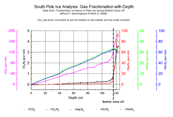 :large
South Pole ice core data shows similar gas composition trends with depth including change in fractionation rate around close-off where the fractionation rate increases.
Furthermore, as my document highlights:
“the authors demonstrate that they cannot reconcile the O2/N2 with the assumed correct CO2 record from ice cores. They find that the O2/N2 data shows fractionation that is about a factor of 4 greater than ‘expected’.”
Thus the ice core dO2/N2 record diverges from the purported CO2 history. http://www.scribd.com/doc/147447107/Breaking-Ice-Hockey-Sticks-Can-Ice-Be-Trusted
Jonathan, the problem is the O2 fractionation, not the CO2 fractionation, which is anyway small and, if present at all, in the order of 0.2-0.4 ppmv.
Did you take into account the change of CO2 in the atmosphere which goes on with depth, which doesn’t exist for other gases?
Latitude
August 29, 2014 at 10:21 am
James, thank you
CO2 levels are the root of the entire global warming hoodoo
Wouldn’t woodoo be a better word?
OK, statistical tests of the annual time series of greenhouse gas (GHG) concentrations and global average temperatures in order to determine if there is a relation between the variables finds that there is one. Huh?
I used the Historical CO2 record derived from a spline fit (20 year cutoff) of the Law Dome DE08
and DE08-2 ice cores for CO2 and my memory for the global temp changes-
The 35 years from 1910 to 1945, CO2 increased from about 300 to 310 ppm (10 ppm) about 3% and temperatures increased about 0.45 degrees C
The 33 years from 1945 to 1978, CO2 increased from about 310 to 333 ppm (23 ppm) about 7% and temperatures fell about 0.1 degrees C
The 36 years from 1978 to 2014, CO2 increased from about 333 ppm to 400 ppm (67 ppm) about 20% and temperatures increased about 0.45 degrees C.
From 1832 to 2014 CO2 increased from about 284 ppm to 400 ppm (116 ppm) about 40% and there was about 0.85 C global warming.
Before I apply any statistical tests, I want to eyeball the data and see if there appears to be a correlation. I suppose statistics is like gerrymandering. By choosing boundaries, you can get the results you’re looking for! The boundaries I choose above show no indication of correlation except the most general. Both CO2 ppm and global temperatures increased over the 1832 to 2014 time period, but not in any consistent way.
For extra credit- what is the inferred climate sensitivity from each of the above data sets?
How about the data set from 1978 to 1998 when CO2 increased from 333- 363 ppm (30 ppm) about 9%, and temperatures increased 0.45 degrees C. Aha, we found one that agrees with the IPCC climate models!
Now we’re cooking!
The Law Dome data is evidence that rising CO2 concentrations are not due to man’s CO2 output. 90% of man’s emissions occurred after 1945, yet the graph shows a steady increase from 1750, the Little Ice Age. There is no sudden increase in recent times. It would seem reasonable to propose that increases in CO2 have been caused by warming from the LIA.
http://www.ferdinand-engelbeen.be/klimaat/klim_img/antarctic_cores_000_3kyr.jpg
no sudden increase ?
I would say that the post 1950 section is a lot steeper in that graph. It’s all roughly exponential in form. If you took the log of the data you would surely get a notably different slope post 1950.
Having said that, that graph is a horrible pastiche of many sources each with their own adjustments and “gas age” guesses, which have very likely been adjusted by cross comparison and ‘corrected’ to fit with later flash measurements.
Ice cores was the first thing I looked into when I started to look more closely at climatology and I quickly found that, although the drilling data in terms of depth and gas analysis is generally well archived, there is a lot of unarchived, undocumented voodoo going on to convert to ice age and particularly gas age.
At that stage the curtain comes down and we’re back to “trust us we know what we are doing”.
Dr Burns, the human emissions were quite small in the period up to 1900, compared to the natural variation, but the increase in the atmosphere after 1900 is directly proportional to the accumulated human emissions:
http://www.ferdinand-engelbeen.be/klimaat/klim_img/acc_co2.jpg
Both accumulated emissions and increase in the atmosphere show a slight quadratic increase over time.
The MWP-LIA cooling shows only a 6 ppmv drop in CO2 for a ~0.8°C drop in temperature in the ice cores. The increase in temperature since the LIA is not more than the MWP-LIA drop, thus should give not more than 6 ppmv extra…
Ferdinand:
You write
That is because your two plotted parameters are each approximately linear with time.
The fact that they are “directly proportional” indicates nothing, suggests nothing, and implies nothing except that they are both approximately linear with time.
Richard
If one plots the accumulation rates over time, it is clear that both are slightly quadratic:
http://www.ferdinand-engelbeen.be/klimaat/klim_img/temp_emiss_increase.jpg
it is also clear that the temperature – CO2 increase relationship is far weaker than between CO2 emissions and CO2 increase. Even during periods of cooling, CO2 levels increase in ratio with the emissions.
Ferdinand
You say
We have been here so very many times before.
There is NO IMMEDIATE DIRECT RELATIONSHIP with anything.
The atmospheric CO2 increase is clearly NOT an accumulation of part of the human emission: in some years almost all of that emission seems to be sequestered and in other years almost none. The most likely explanation for the CO2 increase is an adjustment of the carbon cycle system towards an altered equilibrium. Some mechanisms of the carbon cycle have rate constants of years and decades so the system is responding to something that was decades ago: the temperature rise from the Little Ice Age (LIA) is the most likely cause of the atmospheric CO2 rise, but the human emission could be the cause.
Richard
Come on Richard, The relationship between CO2 emissions and CO2 increase in the atmosphere is very clear and supported by all known observations: mass balance, 13C/12C ratio, 14C bomb spike decay rate, oxygen balance,… Every alternative explanation like extra ocean releases violate one or more observations.
It is not because the “noise” of the year by year uptake is between 10% and 90% of human emissions (even if it was -100% to +200%) that that invalidates the cause: one can statistically calculate the sea level increase within the 1000 times higher noise of waves and tides, even if that needs 25 years of data.
Mosh,
Look at the graph at joelobryan August 29, 2014 at 10:38 am
Why the blip?
JF
Ferdinand,
How long should a CO2 excursion last before it is visible in sponges/stomata? (that must be two different numbers BTW.) How long would a transient blip in atmospheric CO2 take to be absorbed into the ocean?
JF
Any change in local CO2 levels over the growing season is directly visible in the stomata data of the next year, according to Tom van Hoof (stomata specialist), but in general one need several years of leaves to average them, depending of the layer thickness over time. For up to a few thousands years, that gives a resolution of less than a decade, for longer time frames up to several hundred years.
Coralline sponges have a resolution of 2-4 years over the past 600 years, The ocean surface waters where they grow follow the atmospheric δ13C levels within 2-3 years.
The decay rate for a CO2 spike in the atmosphere above equilibrium is over 50 years, or a half life time of ~40 years. See e.g.:
http://www.john-daly.com/carbon.htm
“Any change in local CO2 levels over the growing season is directly visible in the stomata data of the next year, according to Tom van Hoof (stomata specialist),”
———————
Ferdinand, ….. are you trying to tell us that all stomata producing vegetation (plants) …. not only possess “memory storage” capabilities for the recording of environmentally sensed information (CO2 ppm quantities) …. but also possess intelligent reasoning abilities that can “recall” the aforesaid stored environmental data and then make a logical decision on “how many stomata per leaf surface area” will be required during the next growing season?
Not my story: that was told to me by Tom van Hoof, who studied stomata data at the Agricultural University of Wageningen (The Netherlands), where the whole stomata story was born.
There may be some truth in that story, as the leaf buds are formed at the end of the growing season. What is measured is that the stomata density and SI (stomata index: % of stomata cells in total cells) are roughly influenced by CO2 levels. Maybe of the previous year or the year they start to grow, doesn’t make much difference…
Anyway it is a proxy, which isn’t influenced by CO2 alone and it gives a reaction on local CO2 levels over land, which are not easy to compare to “background” CO2 levels…
Here a typical calibration line for two types of oak leaves in SE Netherlands over the past century against ice cores and Mauna Loa CO2 levels:
http://www.ferdinand-engelbeen.be/klimaat/klim_img/stomata.jpg
Interesting paper, but isn’t it sort of self-refuting after only 14 years? The curve in his figure 3 shows atmospheric CO_2 reaching 400 ppm after 2050 and saturating around 420 ppm. In reality, it is 2014 and it is already roughly 400 ppm. In fact, it has increased slightly faster than the solid straight line in this figure (which has it reaching 400 ppm in roughly 2020) which is in accord with Mauna Loa data and data you present above — atmospheric CO_2 is increasing roughly quadratically.
Or, does this figure assume a constant input where the actual input is itself increasing? I mean, I like the model (I would have made it a linearized capacitance model if I were doing it even though I’m not an electrical engineer, but I do teach this stuff to future engineers and his point about the multiple-sink lifetime being dominated by the SMALLEST time constant and being REDUCED by additional parallel channels is entirely apropos).
It also seems as though Trenberth’s assertion that there is sufficient deep ocean mixing to take up the “missing heat” implies that there is sufficient deep ocean mixing to maintain exponential flow of CO_2 into the deep, cold ocean to be sequestered for a hundred thousand years or so.
I have never found the Bern model particularly convincing, but as long as everything proceeds slowly and smoothly we won’t have any actual data to do much better. What we “need” is a discrete accident of some sort that injects several Gt of CO_2 directly into the atmosphere as a bolus so that we can watch/compute the saturation curve, which would contain the time constant. As it is, we are increasing the flow into the reservoir at a rate that prevents it from ever saturating, riding up the slope so that the relaxation time constants are obscured by the time dependence of the input. Sure, in principle one can do deep calculus to extract them from the observed function now, but this relies on knowing the inputs (at least) to very high precision and is going to be an entirely model dependent result — which is IIRC Richard’s point. There is secondary support for at least some aspects of the Bern model, but it isn’t clear what linear models remain viable given the data. I have yet to see a truly convincing presentation on this in all of the discussion of (predominantly ocean) sequestration as everybody makes assumptions that aren’t AFAIK soundly based on accurate measurements or that cannot be supported or refuted by Mauna Loa given a smoothly increasing input.
If you have a better quantitative treatment of this, I’d be very interested.
rgb
rgb, Peter Dietze’s Fig. 3 curve was based on a constant emission of 7 GtC from 1950 on, which is purely theoretical as the real emissions still go on at an increasing rate per year, which is what the fine “cumulation line” in his figure shows.
The remarkable point is that Dietze’s estimate of the overall e-fold decay rate of the extra CO2 in the atmosphere was about 55 years in 1997 when he wrote that paper, while the current e-fold decay rate of the extra CO2 pressure vs, the net sink rate is ~51.5 years, 17 years later…
That means that contrary to the dire predictions of some IPCC members several years ago of a saturation of the deep oceans, that didn’t occur and that vegetation is an increasing sink… Which is bad news for the Bern model and good news for the plants on earth…
Using CO2 to validate CO2 is silly. What about C14 or other techniques to determine the actual ice age?
There are lots of techniques used to determine ice age and gas age. In general, the age of the ice is easier to detect, as there is a difference in density and conductivity between winter and summer layers. Also dust inclusions from known volcanic outbreaks can be used as age markers.
For the ice age – gas age indeed 14C is used and other isotopes like 40Ar and 15N, but still there are a lot of problems to determine the exact age difference and thus the average age of the CO2 levels.
Is there a difference in the quantity of CO2 that is being “trapped” by falling snow verses wind-blown snow?
Is there a difference in the quantity of CO2 that is being “trapped” by “wet” snow verses “dry” snow?
Is there a difference in the quantity of CO2 that is being “trapped” by extremely large or “cluster” snowflakes verses very small or granular snowfall?
Curious minds would like to know.
And just how does one account for the potential surface “melting” of the glacial snowfall and/or glacial ice?
Greenland and other glaciers have been highly subject to said potential surface “melting” during the past 25,000 years.
Samuel, I don’t think that there are differences in CO2 level for different types and quantities of snow (except wet, because of the solubility in water), because there are continuous air and thus CO2 exchanges with the surrounding air.
If there is a remelt layer, then the air under the remelt layer are isolated from the atmosphere and the levels don’t change anymore, while with open pores, the CO2 levels may integrate to the (increasing) level of CO2 in the atmosphere, be it slower and slower with decreased porosity in the depth, until the pores are too small to allow migration…
Ferdinand – simp-ly look at CO2 concentrations in and around Paris, and look at fluctuations over time. Do you think that local fluctuations were unlikely during WWII in Germany. Also note that Poonah and Alaska were both staging areas during WWII. You are expecting instant mixing to provide stable concentrations. I am suggesting that it doesn’t work that way. The unstable WWII sites have recent readings very similar to worldwide averages.
murrayv, I think you have misunderstood me: I do know that such local data like at Poonah and Giessen which make the bulk of the 1942 “peak” in the late Beck’s data should never be used to compile the historical background levels.
I had years of direct discussions with him until his untimely death. I had convinced him to discard the ugly data from Barrow, where the accuracy of the apparatus was +/- 150 ppmv, but couldn’t convince him that the data from Poonah and Giessen were near as bad…
There is a modern station at Linden/Giessen, not far from the historical site where the small town didn’t change that much over time (except for the number of cars I suppose). Here a few summer days (with inversion) out of the CO2 life of Giessen, compared to the (raw!) data from Barrow, Mauna Loa and the South Pole for the same days:
http://www.ferdinand-engelbeen.be/klimaat/klim_img/giessen_background.jpg
two out of three historical samples per day were taken at the flanks of the peaks, the third at the low day level (photosynthesis). That alone gives already a bias of +40 ppmv…
Question: should we use the Giessen data in any compilation of “background” CO2?
I went from
> Jaworowski to Beck, to RC on Beck, to Law Dome, and to
> several other sources. Seems to me that most all are right, and most all
> are wrong. To wit:
> Both Jaworowski and Beck seem to think that the measurements Beck presents
> are global, and therefore ice cores are wrong. They also are thinking
> statically rather than dynamically. RC agrees and points out, corectly,
> that there was no CO2 source that could create the 1942 peak (globally).
> Beck says the peak is not WWII because there are elevated readings in
> Alaska and Poona India.
> Let’s assume that the warm spell peaking about 1938 made a small
> contribution and WWII made a large contribution. There is no reason that
> there couldn’t have been local spikes also in Alaska (military staging)
> and Poona (industrialized part of India supporting the Asian campaign).
> Most of the measurements were from Europe, and in ’41/’42 Europe was in
> flames. Imagine a high ridge of elevated CO2 across Europe that is
> continuously flowing out to become well mixed around the world. By the
> time it gets to the South Pole 200 ppm would probably be no more than 20
> ppm.
> Now consider that a few year spike (bottom to bottom 1935 to 1952) gets
> averaged out over abouit 80 years during ice closure, so its maybe 4 ppm.
> By the time the core is made, 1942 ice is deep enough to form CO2
> clathrates, but not oxygen or nitrogen per Jaworowski, so when the core
> depressurizes, some more of the peak is lost, now 1 ppm.
> Now see Law Dome, per Etheridge “flat to slightly up and down” from about
> 1935 to 1952.
> You can take the Law Dome CO2 plot, look only at the last 100 years, and
> fit Beck’s peak right on the unexplained flat.
> There was plenty of CO2 to generate that ridge over Europe, and it was
> WWII. Beck is right, the ice core is right, RC is right; Beck is wrong, RC
> is wrong, but the ice core remains right.
> It would be nice if people didn’t jump to conclusions and would think
> dynamically.
murrayv
You assert much certainty over matters that are not known. For example, you write
As is usual, RC is not correct.
Almost all the CO2 in the world is in the ocean. A small change in pH of the surface layer would alter the equilibrium concentrations of CO2 in the air and in the ocean. Such a change cannot be obtained by additional dissolved carbon because of the carbonate buffer. However, an injection of dissolved sulphur would do it, and undersea volcanoes may have injected a sulphur pulse into the ocean. Nobody can know if this happened or not, but if it did then the 1942 peak could have resulted.
So, it is a matter of opinion whether the pulse is real or an artifact of the measurements. Nobody knows but some claim to know.
Richard
Richard, there is a pure theoretical possibility that the oceans provided the 1942 peak in CO2 of Beck’s compilation in only 7 years (but not seen in any other indication, including your beloved stomata data), if they suddenly increased in acidity.
But there is not the slightest possibility that the same oceans or any other sink removed that peak in only 7 years again. We are talking about the equivalent of 1/3rd of all land vegetation as release and uptake…
Ferdinand
You are right when you say
except that I DON’T thing the stomata data is “beloved”: It think it has equal but different usefulness to the ice core data.
All of this stuff is “pure theoretical possibility”.
But you are wrong when you write
This is the Mauna Loa data and it shows that for 6 months of each year the net (n.b. net and net total) sequestration rate is sufficient. An assumed reduction to emission – not an assumed increase to sequestration – solves your problem.
Richard
Richard, the 70 ppmv extra CO2 in the atmosphere since Mauna Loa started didn’t change the seasonal variation that much and only caused an extra uptake of 0.7 ppmv/year (1.5 GtC/year) out of the atmosphere.
Therefore it is impossible that the 80 ppmv 1942 “peak” in Beck’s compilation was removed by vegetation in only 7 years. Moreover that would give a huge fingerprint of δ13C changes in both ice cores and coralline sponges. The latter have a resolution of 2-4 years in ocean surface waters, which follow the δ13C changes of the atmosphere within 1-3 years. But there is nothing special to see around the 1942: only a monotone drop in δ13C in ratio to the human emissions.
Neither is it possible that the oceans did take the extra CO2 away in such a short time: the surface is limited in capacity to 10% of the change in the atmosphere and in fast equilibrium, the deep oceans are limited in exchange rate and uptake speed: the current 120 ppmv extra (of which 70 ppmv since Mauna Loa) only give 3 GtC/year extra uptake in the deep oceans.
If the peak was caused by increased acidification of the oceans, what then caused the reduction back to “normal” alkalinity of the oceans? Even massive dissolution of carbonates (which is not noticed in any part of the world for that period) would only restore the alkalinity and the “normal” uptake speed of CO2, which is too slow to remove the “peak” in only 7 years.
That means that the 80 ppmv 1942 peak in Beck’s compilation simply didn’t exist and is only the result of using series which are completely unsuitable to derive background CO2 levels of that time…
Sorry, Ferdinand, but you are wrong.
Anybody can use the link I provided to the MLO data and see that the net sequestration is ~8ppmv for 6 months of each year. And net emission is more than that for the other six months. It is the difference between these half-year periods of net emission and net sequestration which provides the annual rise of each year.
Clearly, variations of 16ppmv in annual net emission and annual net sequestration are hypothetically possible. Thus, you are wrong in two ways when you write
The 80 ppmv 1942 “peak” in Beck’s compilation is not “impossible”
and
your assumption that the CO2 removal from the air would be purely vegetation is wrong: the postulated addition to the air and the postulated removal from the air each results from a change to the equilibrium between air and oceans (although oceanic biota play a large part in this).
I am talking about possibilities which the available data allows.
You are talking about possibilities which your prejudices assert are “impossible”.
Please remember that every part of the AGW scare is based on the assumption that “Nobody can think of anything else” for atmospheric CO2 rise, for global temperature rise, for …etc.. I am saying I can think of other possible attributions, and any other open-minded person can, too.
Richard
Richard, it seems difficult to show you that what you say is simply impossible.
It is -theoretically- possible that the acidification of the oceans should give an extra peak of 80 ppmv in the atmosphere, as the driving force of a lower pH is very huge. But even if the pH returned to “normal” in the subsequent 7 years, it is impossible to push the extra 80 ppmv (170 GtC) back into the oceans (or vegetation) in that time frame.
The current uptake by the (deep) oceans is 1.5 ppmv/year as result of a pCO2 difference of 400 – 250 = 150 μatm between current atmospheric level and cold oceanic temperatures (including biolife) near the poles.
Even if the polar cold waters reduced its pCO2 to zero, the maximum uptake only increased to 4 ppmv/year in the first year, decreasing over time as the pCO2 level in the atmosphere decrease. Thus at least some 30 years that the increased levels should be measurable, that is over 10 years into the Mauna Loa sampling, which show only monotonic increases.
Thus either Beck’s 1942 peak doesn’t exist, consistent with all other indications, or his compilation after 1950 is wrong, as that indicates the same CO2 levels as in ice cores.
We know that the two main series he used which are largely responsible for the 1942 “peak” are heavily biased to higher values and show extreme diurnal variability both today as in the historical samples (Giessen: 68 ppmv – 1 sigma).
We know that both series show no correlation with current or historical “background” CO2 levels.
For all indications, the 1942 “peak” in Beck’s compilation never existed in reality.
I’d like to insert myself briefly into this remarkably polite and courteous disagreement on Ferdinand’s side (sorry Richard). The wiggle in Mauna Loa is clearly a response to an environmental modulator of the oceanic uptake with the periodicity of a year. Almost without any doubt, this is some mix of temperature variation and insolation projected out on sea surface and global vegetation. Much as I truly love fluctuation-dissipation, one cannot conclude that the period of a harmonic component that modulates uptake is itself an exponential time constant. , cooling rates are highly nonlinear as this concentration and atmospheric pressure and things like cloud cover and humidity vary, yet the models attempt to linearize this on 100 km square chunks a km thick as if they have well-mixed concentrations throughout.
To put it in simple terms, imagine that the system is a damped, driven oscillator, e.g. an LRC circuit. Over time, the system will come to oscillate with the frequency of the driver. That frequency is completely independent of the damping resistance. It is not at all trivial to take the behavior of such an oscillator only and make any inferences at all about the effective resistance/damping RC time constant — it requires additional knowledge. This isn’t just an idle example — one can actually view the system as a damped, driven oscillator with a slowly varying DC component that is shifting the “charge” stored on the capacitor up while also making it bounce a bit.
That knowledge (about the damping times) could easily be obtained if the system were hit with a “sudden” forcing — a huge bolus of CO_2 delivered in a very short time to seriously change the persistent disequilibration of the atmosphere with all sinks. The resulting transient behavior as the system returns to a “steady state” behavior consistent with the slowly varying driving plus annual modulation would — if it persisted long enough — permit at least the first few linearized time constants to be extracted from the data via fluctuation-dissipation. As it is now, there ain’t no fluctuations, so it is very difficult to determine the dissipation.
I do happen to think that it is unlikely that the ocean’s exponential lifetime in the multichannel system — as the only really large “ground” sink capable of taking up the additional CO_2 without itself saturating (and hence no longer behaving linearly) is only 7-8 years. There may be reservoirs in the system with time constants this small, but they are likely to have capacitance commensurate with the atmosphere itself and hence are unable to act as a “ground” to it.
Either way, we can all agree that one of the fundamental problems with climate science is the enormous difficulty of determining the precise time dependent past state of the Earth in any time frame prior to the satellite era and modern solid-state instrumentation capable of sampling in many places at high precision. Even where we have data like Beck’s that is reliable from the point of view of the instrumentation, we have far, far too sparse a set of sample sites and some unknown number of those sites are likely to be biased in some equally unknown way. The point is that even if one KEEPS e.g. Poona in Beck’s data, the error estimate for the average should reflect both this and the enormous sparsity of the sampling compared to the surface area of the earth times the height of the atmosphere. All it really tells us is that CO_2 levels near the ground are highly variable and do not necessarily reflect the concentration of “well-mixed” CO_2 a kilometer up and higher.
This itself is not irrelevant to the climate discussion, because most climate models presume “well-mixed” CO_2 all the way to the ground and “most” of the greenhouse warming or lack thereof arises from the CO_2 in that first kilometer, so the models should really be integrating atmospheric radiation rates against things like the Poona curves (something that is probably completely impossible at the current model resolutions, of course). Because of the
In time, this sort of question will eventually be resolved. It won’t be easy, though. Even things like forest fires or Iraq’s torching of oil wells in the 90’s don’t show up as so much as a blip on Mauna Loa compared to the tiny bit of “noise” already visible as a weak variability of the otherwise smooth curve underneath the annual oscillation. In WWII it isn’t even clear that things like the firebombed and nuclear-bombed cities would have produced enough of a pulse to be visible, especially since the pulse itself is subject to yet another exponential time constant, the atmospheric mixing rate, that smooths it out so that it isn’t actually a square pulse by the time it reaches Mauna Loa. It would actually be simpler if we could “discretely” turn off all sources of CO_2 for six months or so and not kill fifty or a hundred million people in the process. That might produce enough of the saturation curve to estimate the leading order time constants.
But even that might not convince the Bern model enthusiasts, as they are asserting a multi-stage oceanic mixing with a very, very long time constant between the low-capacitance surface water and the high-capacitance deep ocean, permitting the sea surface to have a short time constant but still be unable to take up all the atmospheric CO_2. Basically, they assert that atmosphere, biosphere, and upper ocean together are being charged up by the burning of CO_2 (which is yes, split up between them all) but that raises their MUTUAL equilibrium, which can only trickle back to “ground” (deep ocean) on century-plus time scales. This assertion is essentially impossible to refute (or affirm) with current data. Even dumping in a bolus or shutting it all down for a decade might not do it. A huge number of very high precision measurements of oceanic state might do it over several decades. As noted elsewhere, the problem is analogous to Trenberth’s problem with asserting that the missing heat is disappearing into the deep ocean. If so, it could be taking the CO_2 with it. Or not.
Since we don’t have much of a theory or model that could explain either one, and have to rely in improbably precise measurements of e.g. deep ocean temperature variation and/or CO_2 concentration (given the current density and resolution of our measurment apparatus and grid) we’ll have to wait for a very long time for the changes to be clearly and believably resolved and all confounding causes for variation to be accounted for.
rgb
rgbatduke
Thankyou for joining the argument between Ferdinand and me that has been raging for many years. We have often been heated but always mutually respectful so I do not understand your saying
I do not see the relevance of your electrical circuit which does not seem to be anything like an analogue of the carbon cycle system except that you say of your circuit
And I say the time constants of several mechanisms of the carbon cycle are not known.
At issue is what is possible in light of the existing very limited knowledge. As I said to Ferdinand
Failure to recognise what we do not know removes the possibility of looking to correct that lack of knowledge.
Ferdinand makes assumptions that even NOAA is not willing to accept concerning exchanges with deep ocean.
I wrote of Beck’s 1942 pulse
Ferdinand replied
And you have replied
Well, yes, that seems to be agreement with my more succinct statement it replies.
Richard
rgb, thanks for your kind words… I was hardened some long time ago in discussions with activists, where a calm approach was far more effective to convince more moderate people and watchers at the sideline while I was under fire with sometimes very harsh personal attacks…
I do like your electric circuit, as the seasonal component is what the AC component does.
Only one remark: in the case of the seasonal in/out fluxes, vegetation is dominant, not the oceans, although also a lot CO2 is going in and out over the seasons. Because the in/out fluxes with temperature are countercurrent for oceans and vegetation, the net result is quite modest: some 10 GtC/K (global average) from 50 GtC in/out of the oceans and 60 GtC out/in of vegetation.
That are of course rough figures, but not far off reality, as based on O2 use/release (vegetation) and δ13C changes (oceans and vegetation).
The thought error that Richard indeed makes is that he thinks that the seasonal variation shows that the capacity of the sinks is large enough to accommodate for all extra CO2, while that is only the AC component of nature, which says next to nothing about the real capacity to accommodate with increased CO2.
Moreover, the seasonal variations are directly temperature driven, while the (more permanent) storages are pressure related, thus in fact caused by different influences. Or the AC and DC components at work…
To take your analogy further: The ocean surface has a low resistance / low capacity circuit for CO2, while the deep oceans have a high resistance / high capacity circuit. There is hardly any exchange between the ocean surface and the deep oceans. Most exchange between the atmosphere and the deep oceans is in less than 5% of the ocean area each way, largely bypassing the rest of the surface layer.
The atmosphere – deep ocean exchanges are estimated at around 40 GtC/year, based on the “thinning” of the human low δ13C contribution from fossil fuels by the high δ13C from the ocean circulation, where outputs and inputs are largely disconnected. And from the 14C atomic bomb testing spike decay rate and other tracers (CFC’s) of more recent human origin.
About the response to a CO2 spike, although we don’t have a short “spike” the continuous increase of CO2 in the atmosphere gives us an idea about the resistance/capacity of all sinks combined:
The current CO2 level is about 110 ppmv above the historical level for the current temperature.
The sink rate for that pressure difference is about 2.15 ppmv/year, which gives a halve life time of slightly over 50 years.
The Bern model is what one can expect for a lot of parallel working RC sinks, but with several caveats: the limited capacity of the ocean surface is real, but there is no sign that the deep oceans are saturating (as the Bern model implies) and the capacity of vegetation is in fact unlimited as that is what we are burning as coal from long past uptakes.
What we see is that there was no change in uptake over the past 100 years: the uptake remained in the same ratio (in average 50-55% of the emissions, in fact in direct ratio to the increase in the atmosphere) over the whole time frame.
The radiation influence of increased CO2 levels in the first few hundred meters over land may not be that high as you think, but that is not my best area of knowledge…
Please see a boiled down presentation of the pre-1958 CO2 data issues,
“Climate DATA change, its wors than we thought: Atmospheric CO2 concentration”
http://hidethedecline.eu/pages/posts/climate-data-change-atmospheric-co2-concentration-286.php
/ Frank Lansner
Frank: a few remarks:
– deposits in ice are in the year the snow did fall, SO4 is not a gas, that are aerosols which follow the ice phase, not the gas phase.
– gas distribution is quite different and is mainly from the last years before the gas is isolated from the atmosphere.
– there is no problem with the 83 years shift of the Siple Dome data. That story originated from the late Dr. Jawarowski, who looked up the wrong column (ice age i.s.o. average gas age) in the table of the Siple Dome by Neftel.
– wind data only can be used for background estimates if there are sufficient data points above 4 m/s and there is a convergence in the data. Unfortunately that is not the case for the Liège and Giessen data.
Why is it that CO2 gas trapped in an air bubble within the ice core is presumed to be representative of its concentration in the atmosphere? Is there really no chemical activity at all with respect to the gas bubble/ice interface?
In ice cores one can find some seasalt deposits and volcanic and sand dusts, depending of distance and wind speed, even bacteria and algue. The inland Antarctic ice cores have less deposits than the coastal ones. In general that gives no problems for CO2 levels or measurements. But for the Greenland ice cores, that gives huge problems: they have frequent highly acidic deposits from the nearby Icelandic volcanoes. These may react with the seasalts (carbonates) in situ and at measuring time, which gives much higher CO2 levels.
Therefore they don’t use CO2 measurements from the Greenland cores and they changed the wet measuring method for CO2 to measurements in the ice by grating it under vacuum or by total sublimation over cryogenic traps to separate all constituents.
Further, there is a (short) overlap between ice cores and direct atmospheric measurements plus measurements of the distributions of gases in firn top down from the surface to bubble closing depth which shows that for CO2 there is no difference in level between still open pores and already fully closed bubbles at closing depth.
and also
– – – – – – – – – –
James McCown,
Your post is a valuable contribution to the critical dialog on the history of atmospheric CO2 measurements and analysis during the period of the instrumental surface temp measurement from ~1860 to 1958. Your post has that rare attribute in climate science technical discussion of being lucid. Thank you.
It appears to me that, being fully aware of the vociferous criticisms of Beck 2009 (and consequent studies) from a broad spectrum of supporters of mainstream IPCC centric evaluation processes, the datasets in Beck 2009 might possibly form the basis of yearly CO2 values which can potentially be legitimately used in conducting cointegration tests with temperature data for the 100 yr period of ~1858 to 1958. All critical issues with any approach like Beck 2009 having biases inherent in forming the historic chemical measured CO2 datasets can be dealt with in the open dialog of science; the open dialog can sort out the lease problematic solution to utilizing such chemical measured CO2 datasets in conducting cointegration tests. Deal with the Beck 2009 dataset issues like we have all seen that legitimate science can openly deal with inherent problems in sunspot datasets, or surface temp instrument datasets, or sealevel datasets or any climate science timeseries dataset going back >160 yrs. => So one could also do that kind of timeseries issue mitigation process to evaluate if and how to use Beck 2009 datasets to do cointegration tests with temperature data for the 100 yr period of ~1858 to 1958.
John
John, thank you for the nice thoughts.
That was in fact already done by Guy Callendar, mentioned by climatereason further on. He used stringent criteria to include or exclude CO2 measurements like “not used for agricultural purposes”, which excluded problematic series like Poonah and Giessen which cause the 1942 “peak” in Beck’s compilation.
One can have objections against some of his criteria, but the opposite, no criteria at all, is far worse…
Decennia later, Callendar’s estimates were proven right by the data measured in ice cores. Even if one takes the historical data which were taken over the oceans or coastal with wind from the sea: these are all around the ice core data…
@ferdinand meeus Engelbeen August 30, 2014 at 12:22 pm
WRT your first point:
Callendar’s questionable extreme selectivity in his dataset that excluded more than a hundred thousand chemical based measurements of CO2 before ~1940 was done many decades before Beck’s (2009) comprehensively expanded dataset that went up to ~1958. It was the surprising lack of any attempt at comprehensive data in Callendar’s dataset that raised a very reasonably based motivation for work like Beck’s.
WRT your second point:
I suggest we try to avoid begging the question. The comprehensive critical view of the pre-industrial level of CO2 leads critics to a very key question about how the ice core data came to be matched to the extremely selective dataset of Callendar. It is an obvious and critical point of contention, so matching is not evidence of the correctness of Callendar or of the ice core researchers.
Going back to the original point of my comment above, I suggest it would be an advance of knowledge if we could use Beck 2009 datasets to do cointegration tests with temperature data for the 100 yr period of ~1858 to 1958.
John
John, one can discuss the criteria which were used by Callendar, like excluding every measurement that differed more than 10% from the most probable level of that time, but as modern measurements show, in 95% of the atmosphere, the difference between near the North Pole and the South Pole is not more than 2% of full scale.
In contrast, Beck used no criteria at all: he lumped everything together, the good, the bad and the ugly. The latter from measurements with an accuracy of the equipment around +/- 150 ppmv, intended for measuring CO2 in exhaled air (20,000 ppmv and more). Fit for that purpose, but by far not accurate enough to have any idea of background CO2 levels of that time…
The work of Callendar and the ice core measurements were completely independent of each other. Given that the historical measurements taken over the oceans match the ice core data, that are two independent datasets which match each other, where Callendar added some more land based data. Unfortunately there are no ocean based data around the 1942 “peak”…
In my opinion, it is of no use to take the compilation by Beck as base for any comparison. Neither is it of any use to take temperature data from the middle of towns or on an asphalted parking lot in any comparison… Only if Beck’s compilation is cleaned for local CO2 biases, that would be of use (which is a hell of a job). If there are modern measurements at the same places as the historical ones, that would already give a better indication of the local biases, as is the case for Giessen…
@JohnWhitman I took a look at Beck’s spreadsheet. The problem is, there are a number of years in the 20th century that don’t have any data at all. But it may be possible to compute 5 year averages and do the unit root and cointegration tests with that.
Ferdinand Engelbeen
August 31, 2014 at 11:30 am
– – – – – – – –
Ferdinand Engelbeen,
That Beck (2009) included a dramatic several orders of magnitude increase in the volume of measurements in his dataset is a clear merit for the advance of science. It is the launching pad of more comprehensive and circumspect research than Callendar’s. Now we have a several order magnitude broader base to promote more knowledge of the Earth Atmosphere System (EAS).
You seem to imply that a several order magnitude increase to a more comprehensive measurement dataset is somehow not better for climate science research to be done on. Why (if that is your implication)?
John
James McCown August 31, 2014 at 1:20 pm
– – – – – –
James McCown,
I appreciate the observation on Beck’s dataset.
John
John Whitman
September 1, 2014 at 11:08 am
More data are not necessary beneficial for knowledge. Much depends of the quality of the data. For equal quality, more data give more knowledge. If the extra data are of worse quality than the sparse data you have, that doesn’t benefit your knowledge, to the contrary…
Take e.g. the surface stations project: quality criteria are necessary to separate the good, the bad and the ugly stations. 100 good stations are much better than a mix of 1000 good and bad situated stations…. Callendar did do that, Beck didn’t do that. With as result that he mixed the good and the bad data and even the ugly ones, which he removed only because we could convince him that these were ugly.
If we want to take advantage of the extra data which were compiled by Beck, we need to go over all the data he managed to retrieve (which was an enormous job), taking into account the current knowledge of good sampling places.
Current good sampling places are over the oceans, coastal with wind from the oceans, in deserts (like the South Pole), high on mountains… Not in the middle of towns, forests, growing crops…
I discussed the data over the period 1935-1955 with him where his second “peak” was situated. There were only a few good sampling places in a few separate years over the whole period. Two of the best places (Barrow and Antarctica) had equipment which was much too inaccurate, which is very unfortunate and the two series which largely make his 1942 “peak” were at places which should never be used for “background” CO2 measurements, as the wide variability in measurements show. Here for Poona, measured by Misra:
http://www.ferdinand-engelbeen.be/klimaat/klim_img/misra_wind.jpg
From November 1942 to July 1943, CO2 levels dropped from 700 ppmv to 300 ppmv. If you think that such a drop is physically possible for “background” CO2 levels, I like to know what mechanism may be behind that…
I can’t comment on the physics of it. But I always did wonder a little that there was not a large CO2 blip during WWII.
Yes, I know that many oil fields were rendered inoperable and available manpower and transportation was always an issue with coal. But not only did the world blow out all its reserves and increased production wherever possible, but the upwards of 100 cities were incinerated or blasted into rubble. The RAF was pleased to refer to this as “terrorisation” and “dehousing”. A large amount of CO2 is released by burning things. And in a war, burning things is a hockey stick.
So I always was a little uncomfortable regarding the issue.
evanmjones
Ironically Guy Callendar played a great part in the British war effort and among other things banished fog from airfields that threatened to seriously disrupt the war effort. He did this by laying large pipes which carried petrol to the runways and then setting fire to the thousands of gallons that were then pumped out.
This apparently drove away the moisture so successfully that it was adopted widely. Presumably it had an effect on the co2 levels he noted in his 1938 Co2 paper which his peers pointed out was incorrect as it was well known that co2 was around 400ppm at that time (courtesy of Callendars archives and biography)
tonyb
If the 1942 spike in CO2 as shown in Beck’s compilation actually happened, then there should be an all-out effort to determine how that spike dissipated as quickly as it did, for obvious reason.
I am curious why there is no indication of WWII or Cold War nuke testing in the data. It seems to me that blowing up millions of pounds of munitions, burning hundreds of thousands of gallons of diesel and petrol, fire-bombing cities, and destroying two cities with nukes, followed by two decades with over two-thousand nuclear tests would produce quite a bit of CO2.
It could have dissipated quickly just because it was measured in non-well-mixed CO_2 near the ground, and took several years to mix with the rest of the atmosphere. Or not. To paraphrase Yogi Berra and indicate the second half of a very big problem with climate science: It’s tough to make measurements, especially of the past.
Tough to make predictions, especially of the future, tough to make measurements, especially of the past, makes it very tough indeed to build models that rely on an accurate knowledge of the past that actually work to predict the future.
rgb
Reference graph @ joelobryan August 29, 2014 at 10:38 am
One thing I also note of interest is the sudden drop of the CO2 level from the early 1940’s blip. Eyeball scaling looks like a drop of about 70 ppm in about 10 years time. Planet Earth may be quite efficient at carbon sequestering. Guess that could put a damper on the supposed long life of CO2 in the atmosphere.
But then as rgb notes, where was it measured?
@eternaloptimist
“any activity that went from a zero baseline, to a peak, then a haitus would fit the bill.”
Our confidence in the accuracy of global temperatures as measured by satellites would fit. From zero when there were no satellites through the beginning of the satellite era where confidence rose and fell depending on the adjustments and error corrections until it leveled off at a high level and has pretty much stayed there since. And AQUA doesn’t even drift.
Added benefit is the irony.
Me thinks that after Keeling started measuring and recording semi-accurate atmospheric CO2 ppm quantities in 1958, ….. then everyone else started their per se, “reverse engineering” of their CO2 ppm proxy data to make sure theirs “correlated” with Keeling’s starting quantities and/or average yearly increases.
The estimated yearly “human emissions” of CO2 has always been based in/on Keeling’s average yearly increases.