This exercise in data analysis pins down a value of 1.8C for ECS.
Guest essay by Jeff L.
Introduction:
If the global climate debate between skeptics and alarmists were cooked down to one topic, it would be Equilibrium Climate Sensitivity to CO2 (ECS) , or how much will the atmosphere warm for a given increase in CO2 .
Temperature change as a function of CO2 concentration is a logarithmic function, so ECS is commonly expressed as X ° C per doubling of CO2. Estimates vary widely , from less than 1 ° C/ doubling to over 5 ° C / doubling. Alarmists would suggest sensitivity is on the high end and that catastrophic effects are inevitable. Skeptics would say sensitivity is on the low end and any changes will be non-catastrophic and easily adapted to.
All potential “catastrophic” consequences are based on one key assumption : High ECS ( generally > 3.0 ° C/ doubling of CO2). Without high sensitivity , there will not be large temperature changes and there will not be catastrophic consequences. As such, this is essentially the crux of the argument : if sensitivity is not high, all the “catastrophic” and destructive effects hypothesized will not happen. One could argue this makes ECS the most fundamental quantity to be understood.
In general, those who are supportive of the catastrophic hypothesis reach their conclusion based on global climate model output. As has been observed by many interested in the climate debate, over the last 15 + years, there has been a “pause” in global warming, illustrating that there are significant uncertainties in the validity of global climate models and the ECS associated with them.
There is a better alternative to using models to test the hypothesis of high ECS. We have temperature and CO2 data from pre-industrial times to present day. According to the catastrophic theory, the driver of all longer trends in modern temperature changes is CO2. As such, the catastrophic hypothesis is easily tested with the available data. We can use the CO2 record to calculate a series of synthetic temperature records using different assumed sensitivities and see what sensitivity best matches the observed temperature record.
The rest of this paper will explore testing the hypothesis of high ECS based on the observed data. I want to re-iterate the assumption of this hypothesis, which is also the assumption of the catastrophists position, that all longer term temperature change is driven by changes in CO2. I do not want to imply that I necessarily endorse this assumption, but I do want to illustrate the implications of this assumption. This is important to keep in mind as I will attribute all longer term temperature changes to CO2 in this analysis. I will comment at the end of this paper on the implications if this assumption is violated.
Data:
There are several potential datasets that could be used for the global temperature record. One of the longer and more commonly referenced datasets is HADCRUT4, which I have used for this study (plotted in fig. 1) The data may be found at the following weblink :
http://www.cru.uea.ac.uk/cru/data/temperature/HadCRUT4-gl.dat
I have used the annualized Global Average Annual Temperature anomaly from this data set. This data record starts in 1850 and goes to present, so we have 163 years of data. For the purposes on this analysis, the various adjustments that have been made to the data over the years will make very little difference to the best fit ECS. I will calculate what ECS best fits this temperature record, given the CO2 record.

Figure 1 : HADCRUT4 Global Average Annual Temperature Anomaly
The CO2 data set is from 2 sources. From 1959 to present, the Mauna Loa annual mean CO2 concentration is used. The data may be found at the following weblink :
ftp://aftp.cmdl.noaa.gov/products/trends/co2/co2_annmean_mlo.txt
For pre-1959, ice core data from Law Dome is used. The data may be found at the following weblink :
ftp://ftp.ncdc.noaa.gov/pub/data/paleo/icecore/antarctica/law/law_co2.txt
The Law Dome data record runs from 1832 to 1978. This is important for 2 reasons. First, and most importantly, it overlaps Mauna Loa data set. It can easily be seen in figure 2 that it is internally consistent with the Mauna Loa data set, thus providing higher confidence in the pre-Mauna Loa portion of the record. Second, the start of the data record pre-dates the start of the HADCRUT4 temperature record, allowing estimates of ECS to be tested against the entire HADCRUT4 temperature record. For the calculations that follow, a simple splice of the pre-1959 Law Dome data onto the Mauna Loa data was made , as the two data sets tie with little offset.

Figure 2 : Modern CO2 concentration record from Mauna Loa and Law Dome Ice Core.
Calculations:
From the above CO2 record, a set of synthetic temperature records can be constructed with various assumed ECS values. The synthetic records can then be compared to the observed data (HADCRUT4) and a determination of the best fit ECS can be made.
The equation needed for the calculation of the synthetic temperature record is as follows :
∆T = ECS* ln(C2/C1)) / ln(2)
where :
∆T = Change in temperature, ° C
ECS = Equilibrium Climate Sensitivity , ° C /doubling
C1 = CO2 concentration (PPM) at time 1
C2 = CO2 concentration (PPM) at time 2
For the purposes of this test of sensitivity, I set time 1 to 1850, the start of the HADCRUT4 temperature dataset. C1 at the same time from the Law Dome data set is 284.7 PPM. For each year from 1850 to 2013, I use the appropriate C2 value for that time and calculate ∆T with the formula above. To tie back to the HADCRUT4 data set, I use the HADCRUT4 temperature anomaly in 1850 ( -0.374 ° C) and add on the calculated ∆T value to create a synthetic temperature record.
ECS values ranging from 0.0 to 5.0 ° C /doubling were used to create a series of synthetic temperature records. Figure 3 shows the calculated synthetic records, labeled by their input ECS, as well as the observed HADCRUT4 data.

Figure 3: HADCRUT4 Observed data and synthetic temperature records for ECS values between 0.0 and 5.0 ° C / doubling. Where not labeled, synthetic records are at increments of 0.2 ° C / doubling. Warmer colors are warmer synthetic records.
From Figure 3, it is visually apparent that a ECS value somewhere close to 2.0 ° C/ doubling is a reasonable match to the observed data. This can be more specifically quantified by calculating the Mean Squared Error (MSE) of the synthetic records against the observed data. This is a “goodness of fit” measurement, with the minimum MSE representing the best fit ECS value. Figure 4 is a plot of MSE values for each ECS synthetic record.

Figure 4 : Mean Squared Error vs ECS values. A few ECS values of interest are labeled for further discussion
In plotting, the MSE values, a ECS value 1.8 ° C/ doubling is found to have the minimum MSE and thus is determined to be the best estimate of ECS based on the observed data over the last 163 years.
Discussion :
A comparison to various past estimates of ECS is made in figure 5. The base for figure 5 comes from the following weblink :
http://www.cato.org/sites/cato.org/files/wp-content/uploads/gsr_042513_fig1.jpg
See link for the original figure.

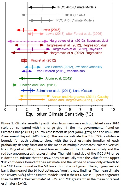
Figure 5 : Comparison of the results of this study (1.8) to other recent ECS estimates.
The estimate derived from this study agrees very closely with other recent studies. The gray line on figure 5 at a value of 2.0 represents the mean of 14 recent studies. Looking at the MSE curve in figure 4, 2.0 is essentially flat with 1.8 and would have a similar probability. This study further reinforces the conclusions of other recent studies which suggest climate sensitivity to CO2 is low relative to IPCC estimates .
The big difference with this study is that it is strictly based on the observed data. There are no models involved and only one assumption – that the longer period variation in temperature is driven by CO2 only. Given that the conclusion of a most likely sensitivity of 1.8 ° C / doubling is based on 163 years of observed data, the conclusion is likely to be quite robust.
A brief discussion of the assumption will now be made in light of the conclusion. The question to be asked is : If there are other factors affecting the long period trend of the observed temperature trend (there are many other potential factors, none of which will be discussed in this paper), what does that mean in terms of this best fit ECS curve ?
There are 2 options. If the true ECS is higher than 1.8, by definition , to match the observed data, there has to be some sort of negative forcing in the climate system pushing the temperature down from where it would be expected to be. In this scenario, CO2 forcing would be preventing the temperature trend from falling and is providing a net benefit.
The second option is the true ECS is lower than 1.8. In this scenario, also by definition, there has to be another positive forcing in the climate system pushing the temperature up to match the observed data. In this case CO2 forcing is smaller and poses no concern for detrimental effects.
For both of these options, it is hard to paint a picture where CO2 is going to be significantly detrimental to human welfare. The observed temperature and CO2 data over the last 163 years simply doesn’t allow for it.
Conclusion :
Based on data sets over the last 163 years, a most likely ECS of 1.8 ° C / doubling has been determined. This is a simple calculation based only on data , with no complicated computer models needed.
An ECS value of 1.8 is not consistent with any catastrophic warming estimates but is consistent with skeptical arguments that warming will be mild and non-catastrophic. At the current rate of increase of atmospheric CO2 (about 2.1 ppm/yr), and an ECS of 1.8, we should expect 1.0 ° C of warming by 2100. By comparison, we have experienced 0.86 ° C warming since the start of the HADCRUT4 data set. This warming is similar to what would be expected over the next ~ 100 years and has not been catastrophic by any measure.
For comparison of how unlikely the catastrophic scenario is, the IPCC AR5 estimate of 3.4 has an MSE error nearly as large as assuming that CO2 has zero effect on atmospheric temperature (see fig. 4).
There had been much discussion lately of how the climate models are diverging from the observed record over the last 15 years , due to “the pause”. All sorts of explanations have been posited by those supporting a high ECS value. The most obvious resolution is that the true ECS is lower, such as concluded in this paper. Note how “the pause” brings the observed temperature curve right to the 1.8 ECS synthetic record (see fig. 3). Given an ECS of 1.8, the global temperature is right where one would predict it should be. No convoluted explanations for “the pause” are needed with a lower ECS.
The high sensitivity values used by the IPCC , with their assumption that long term temperature trends are driven by CO2, are completely unsupportable based on the observed data. Along with that, all conclusions of “climate change” catastrophes are also completely unsupportable because they have the high ECS values the IPCC uses built into them (high ECS to get large temperature changes to get catastrophic effects).
Furthermore and most importantly, any policy changes designed to curb “climate change” are also unsupportable based on the data. It is assumed that the need for these policies is because of potential future catastrophic effects of CO2 but that is predicated on the high ECS values of the IPCC.
Files:
I have also attached a spreadsheet with all my raw data and calculations so anyone can easily replicate the work.
ECS Data (xlsx)
=============================================================
About Jeff:
I have followed the climate debate since the 90s. I was an early “skeptic” based on my geologic background – having knowledge of how climate had varied over geologic time, the fact that no one was talking about natural variation and natural cycles was an immediate red flag. The further I dug into the subject, the more I realized there were substantial scientific problems. The paper I am submitting is a paper I have wanted to write for years , as I did the basic calculations several years ago & realized there was no support in the observed data for high climate sensitivity.
This simplistic and faulty analysis assumes that the Hadrut temperature record is a true representation of World temperatures over the period shown. In fact, the Hadcrut graph, like all similar ones is the result of continuous ‘adjustment’ to increase recent temperatures and reduce past temperature records. Most recent temperature increases are solely the result of beneficial ‘adjustments’.
Basing a comparison and sensitivity between CO2 levels and temperature also assumes that there are no other influences at all (like the Sun) on Earth’s average temperature. Coming up with a figure of 1.8 or the IPCC 2.1 or the alarmist 4 is just folly.
First one has to establish what are the real influences on Earth temperature and then work back to their likely effects, not assume that it is just CO2 and attribute ‘adjusted’ temperature rise to that.
REPLY: Then go do it, but in the meantime your comment is little more than whining – Anthony
Simple and elegant.
Thermal mass seems to be ignored.
You can’t calculate an equilibrium value without a thermal mass unless you assume the thermal mass is negligible – making the instantaneous value the equilibrium value. Considering the amount of water on the planet, it seems unlikely that the thermal mass of the planet is negligible.
And, of course, the oceans move heat spatially and temporally. The simplest acceptably accurate solution to a problem is definitely the best one, but this solution is too simple, too inaccurate.
The assumption relating to climate sensitivity to carbon dioxide is dependent upon an assumption that there would be uniform temperatures in the troposphere in the absence of moisture and so-called greenhouse gases. GH gases are assumed to establish a “lapse rate” by radiative forcing and subsequent upward convection.
In physics “convection” can be diffusion at the molecular level or advection or both. It is important to understand that the so-called “lapse rate” (which is a thermal gradient) evolves spontaneously at the molecular level, because the laws of physics tell us such a state is one with maximum entropy and no unbalanced energy potentials. In effect, for individual molecules the mean sum of kinetic energy and gravitational potential energy is constant.
So this thermal gradient is in fact a state of thermodynamic equilibrium. If it is already formed in any particular region then indeed extra thermal energy absorbed at the bottom of a column of air will give the impression of warm air rising. But that may not be the case if the thermal gradient is not in thermodynamic equilibrium and is initially not as steep as it normally would be. In such a case thermal energy can actually flow downwards in order to restore thermodynamic equilibrium with the correct thermal gradient.
What then is the “correct” thermal gradient? The equation (PE+KE)=constant amounts to MgH+MCpT=constant (where M is the mass, H is the height differential and T the temperature differential and Cp the specific heat.) So the theoretical gradient for a pure non-radiating gas is -g/Cp as is well known to be the so-called dry adiabatic lapse rate. However, thermodynamic equilibrium must also take into account the fact that radiation could be transferring energy between any radiating molecules (such as water vapour or carbon dioxide) and this has a propensity to reduce the net result for the thermal gradient. Hence we get the environmental lapse rate representing the overall state of thermodynamic equilibrium.
This can’t be! The data agrees with the conclusions! (sarc off)
The simple fact is this; warmists believe that traces of CO2 generated at ground level by the burning of so called “fossil fuels” make the implausible journey to the upper atmosphere and cause CAGW – they have NO other position whatsoever, and since despite their mantra and models, recent GW has ceased for 17.5 years, they have NO position whatsoever.
Case proven and closed, time to get a real job and stop wasting the taxpayers money!
Good work. But the assumption that I find almost universal and, to my mind, the most unlikely, is that CO2 emissions will continue at the current rate. Look at the full range of assumptions
that simple assumption requires : that electric cars will not replace current ICE vehicles for many decades; that electricity will not be increasingly produced by non-CO2 emitting generators (especially nuclear, which is experiencing unprecedented adoption in India, China, the Middle East, South America, Britain, etc, places where a large portion of the CO2 emission sources are located), that natural gas will not continue to replace most coal generation, or alternatively, that the non-emitting coal combustion process developed at Ohio State will not become commercialized).
That CO2 emissions will remain the same for the extended future I find utterly implausible and
practically impossible. Time and technology marches on. Always has, always will.
ntesdorf: I suppose if you find the analysis simplistic and faulty, you might as well criticize it on the same basis, which you seem to have done quite nicely.
[snip – waaaaaaaaaaayyy off topic – Anthony]
I always suspect calculations based on 100 plus years which eliminates the historical earth climate. Other warm periods in time plus the various ice ages. However I do understand in the AGW camp CO2 as THE factor. What I don’t get is why we always fall into the AGW trap and only concentrate what the AGW camp wants us to talk about, CO2. Something melted each ice age long before man ever existed. I know, I know – trying to prove man is entirely responsible is the buzz words. With respect – I don’t trust any temperature massaged so many times none of us know what real temperature were or supposed to be anymore. Even the different data collected by different device cannot agree with each other and have to be massaged.
Well, setting aside the raging debate on the credibility of the data set being used, this is assuming that ALL influences on global temperature are solely attributable to carbon dioxide concentrations, which I presume most sincere people would doubt. However, as a tact to take while in a bar debating the severity of anthropogenic global warming, I fully support its simplicity in pointing out the flaws of an alarmist’s argument for catastrophe.
I hate to be the guy throwing cold water, but that method needs to be tested on out-of sample data. All you’ve done up there is a simple fit of CO2 to temperature. I can do the same thing with the cost of US postage stamps, and get the same level of significance. Or I can do it with population, or with the cumulative inflation rate … so what?
As a first test of your results, you need to do an “out-of-sample” test by doing the following:
1. Divide your data into 3 periods of ~ 50 years each.
2. Fit the CO2 increase to the temperature in each of the periods separately.
3. Apply the “climate sensitivity” you found in step 2 to the other two segments of the data and note how poorly they fit.
Give that a shot, report back your results …
w.
‘In general, those who are supportive of the catastrophic hypothesis reach their conclusion based on global climate model output.”
Wrong. Hansen for example relies on Paleo data.
REPLY: and I call BS on your “wrong”
From Hansen’s “paper”:
Hansen, J., 2007: Climate catastrophe. New Scientist, 195, no. 2614 (July 28), 30-34.
A sea level rise of several metres will be a near certainty if greenhouse gas emissions keep increasing unchecked. Why are scientists reluctant to speak out? http://pubs.giss.nasa.gov/docs/2007/2007_Hansen_2.pdf
– Anthony
“Hansen for example relies on Paleo data.”
But who relies on Hansen? Anyone? [I mean, anyone rational.]
Here’s Siple vs Mauna Loa. I wouldn’t be surprised if Law Dome has also been faked.
http://www.ferdinand-engelbeen.be/klimaat/klim_img/siple1a.jpg
I saw no formulas in the “modeled temps” tab of your spreadsheet, but I infer from your discussion that you assumed no delay. My understanding of “equilibrium climate sensitivity” is the temperature increase that results after the C02 concentration has reached double and remained there indefinitely.
In other words, proponents of high equilibrium client sensitivity would say that temperatures would continue to climb even if CO2 concentration remained fixed; it would approach the equilibrium value asymptotically.
This means you need at least two parameters (only two if you assume a first-order linear system): equilibrium climate sensitivity and time constant, or, as vboring put it, thermal mass.
The article ignors the fact that CO2 changes are a result of warming rather than a cause.
A perfectly reasonable analysis as far as it goes. It suffers from the usual — the assumption that CO_2 is the only knob is almost certainly false. For example, would anyone care to take the model and hindcast the Little Ice Age from it? How about the Medieval Warm Period? We know that the climate varies naturally by order of 1 C or more on a century time scale. Indeed, if one looks even at HADCRUT4:
http://www.woodfortrees.org/plot/hadcrut4gl/from:1800/to:2013/plot/hadcrut4gl/trend
The rule rather than the exception is for the climate to vary by 0.1C or more over a decade. Furthermore, the rule rather than the exception is for the climate to vary by 0.1/decade or more over multiple decades in a row in a single direction.
How anyone could call the stretch from 1970 to 2000 “unusual” is beyond me, when the stretch from 1910 to 1940 is almost identical in structure and span.
Note well that CO_2 did not descend or remain neutral from 1855 to 1910, or from 1950 to 1970, or from 2000 to the present, but the climate did.
Basically, one simply cannot look at the temperature record anywhere and ascertain how much of any given stretch of temperature or its variation occurs due to “natural” causes and how much occurs due to variations in atmospheric GHG chemistry. No simple model fits (even when reasonably well done, as this one is) can accomplish it. Neither, apparently, can predictive models.
rgb
It seems to me there is a fundamental mental error being made if one considers the ECS as anything but the net end result. The author discusses the possibilities of a high ECS with negative forcings keeping temperatures lower, and a low ECS with positive forcings keeping temperatures elevated. I see the ECS as the final result of all the forcings, negative and positive, on the global temperature. If the temperature and CO2 observations suggest a value of 1.8, then that is the true value. Period. The end.
In a complex system like the climate, wouldn’t all of the myriad variables and forcings mingle to determine how the climate reacts to increased CO2, and then that would BE the ECS? Maybe I’m seeing it wrong, and I would certainly appreciate seeing where I’ve made my error.
The problem with this analysis is that it assumes that all warming is caused by CO2, which is obviously wrong when viewing the HADCRUT plot. There is clearly a natural components which caused warming in early 1900s, and some cooling 1940-1970. It is faulty logic to make an assumption that is wrong, and then declaring that if there is a natural component then the situation is even better. In fact, addition of a natural component that suggests a higher ECS, is not a good thing because we don’t know what are the future natural drivers to the climate. There may be in the future natural warming added to CO2 forcing.
So the error here is that we are suggesting we know something, when in fact we don’t. We face an unquantified future risk (it may be bad, it may not be). When we acknowledge this uncertainty, it is wrong to be panicking and declaring that we face certain doom unless we dismantle our energy technology base, but fooling ourselves into believing everything is OK is also self-deceit.
I would encourage the author of this essay to do the analysis again for a range of assumptions of natural climate change vs CO2 forcing see what results. Instead of pinning down a value for ECS, I suggest it would probably result in a wide range of values. But I believe it would be a worthwhile venture, if only to show the impact of assumptions of natural vs human induced in this debate.
“The big difference with this study is that it is strictly based on the observed data. There are no models involved and only one assumption – that the longer period variation in temperature is driven by CO2 only.”
Well there MUST be some natural variability in there as well. So the figure could be lower (or higher) than that quoted.
http://i29.photobucket.com/albums/c274/richardlinsleyhood/Fig8HadCrutGISSRSSandUAHGlobalAnnualAnomalies-Aligned1979-2013withGaussianlowpassandSavitzky-Golay15yearfilters_zps670ad950.png
1. to calculate ECS you have to include OHC ( or assume) that OHC is zero.
in other words, ECS implies that the system has reached equillibrium. So since the
system has not, you need to have an estimate for delta OHC.
2. If you do not include delta OHC, then you are estimating something closer to TCR
TCR is roughly 1.3 to 2.2 so your estimate is in line with this
Next, to do the estimate properly you need all Forcing
use all forcing to give you lambda.. the system response to all forcing
from lambda you can calculate the senitivity to C02 doubling
I concur with what Willis stated, but I propose you take your simple analysis a little further. Show us a graph of the deviation of the “actual” temperature record from the “1.8” calculated record, then calculate the simple statistical values that determine the “cause/effect” certainty of your “model”. Second, you need to turn the whole concept on it’s head and ask the question, does the temperature record cause the CO2 change instead of vice versa. Others have proposed and documented with a fair degree of certainty that the integral of the actual temperature trends predict the current CO2 values.
IMHO temperature drives CO2 increase and the burning of fossil fuels is dwarfed by simple outgassing from the integral effect of accumulated ocean warming. More importantly than that, you are falling into the trap of arguing about the “noise” when in fact on any given day/month/year temperature changes far above 1 or 2 degrees in spite of a relatively CONSTANT CO2. There is NO temperature signal at Mauna Loa that matches the annual cyclical CO2 concentration signal!
There are a number of factors of unknown magnitude that render any attempt to derive the right value of sensitivity in the manner done here essentially impossible.
To begin with, a proper model must recognize that the real Earth has thermal inertia. This means, at the very least, one needs to use a differential equation of the form:
T = sensitivity*Forcing -response time*dT/dt
The second problem is that one needs to recognize that more forcings other than CO2 act on the temperature record. These include volcanic eruptions, variations in solar brightness, other greenhouse gases (such as methane, CFCs, N2O, etc), dynamically induced non feedback variations in cloud cover, sulphates, black carbon, land use change, and many, many more factors, most of which are highly uncertain.
The third problem is uncertainty of the temperature record itself-how much of the change is real versus due to data biases?
The fourth problem is non linearity of sensitivity-that is, df/dT, where f represents the rate of radiative heat loss, is not a constant, as various effects can increase or decrease the change of rate with temperature at higher temperatures.
All of these problems make attempting to estimate the sensitivity in this way pretty much a pointless exercise. Something that would make more sense would be to attempt to estimate the magnitude of the feedback response, which overcomes every problem except the fourth.
Of course, if you do that, you’re going to get an answer that’s like a third what you’re getting here. But given all the problems with this approach, that’s not that surprising.
The most significant evidence we have of low sensitivity is the pause. The alarmist need the heat to be in the ocean. They need it or they know it is game over.
If we have perfect measurements from satellites of the input and output heat radiation budget then we will know if heat is in ocean.
My guess is that there is a big negative feedback mechanism we do not fully understand. There is some type of release valve , throttle as Willis says. It has to do with water cycle or wind in my opinion.
Here you go, it’s the secret of climate that we’ve searched for so long …

SO … I can use that to calculate the climate sensitivity of the relationship. Just like the head post, I’ve used the log of the underlying data (to base 2, as in the head post).
Only problem?
The red line is not CO2. It’s the CPI, the Consumer Price Index, since 1850 …
Jeff, I hope you can see that this type of “match up the curves” is not all that diagnostic …
w.
PS: If you truly want to do this kind of analysis, you need to use a lagging equation on your forcings, and you need to include all known forcings. The problem is, most forcings we have no clue about for the 1800’s … so we end up with error bars (which you’ve neglected) from floor to ceiling.
Jeff, what is your uncertainty estimate, plus/minus degrees C ?
Also what you are estimating is the transient climate response since it will take additional time for the oceans to adjust to changes in temperature.
Continuing from my comment at 2:16pm, the inevitable conclusion is that it is not greenhouse gases that are raising the surface temperature by 33 degrees or whatever, but the fact that the thermal profile is already established by the force of gravity acting at the molecular level on all solids, liquids and gases. So the “lapse rate” is already there, and indeed we see it in the atmospheres of other planets as well, even where no significant solar radiation penetrates.
In fact, because the “dry” lapse rate is steeper, and that is what would evolve spontaneously in a pure nitrogen and oxygen atmosphere, and because we know that the wet adiabatic lapse rate is less steep than the dry one, it is obvious that the surface temperature is not as high because of these greenhouse gases. Carbon dioxide (being one molecule in about 2,500 other molecules) has very little effect, but whatever effect it does have would thus be very minor cooling.
I don’t care what you think you can deduce from whatever apparent correlation you think you can demonstrate from historical data, there is no valid physics which points to carbon dioxide warming.
You are looking at transient climate response (TCR), not equilibrium climate sensitivity (ECS). The IPCC AR4 TCR numbers are 1.5 to 2.8 C per doubling of CO2, with a mean estimate of 2.1. In the AR5, the average TCR across CMIP5 models was 1.8 C per doubling. So technically your result ends up being exactly the same as the models :-p
Mosher says
“‘In general, those who are supportive of the catastrophic hypothesis reach their conclusion based on global climate model output.”
Wrong. Hansen for example relies on Paleo data.”
Really Mosh? No one has ever shown any DATA that demonstrates that CAGW is real. That is the problem, if there was DATA that demonstrates that, there would be no issue whatsover. with us skeptics, except for perhaps on how to address/solve it. CAGW currently exists ONLY in the models. Hansen does not rely on Paleo data to prove CAGW. Perhaps he uses paleo data, sticks it into his MODEL, and viola!…. CAGW.
Aslo, if you are mentioning Paleo data because of the recent paper. I scanned through the paper and saw no graphical presentation of any of the temperature data the were fitting the models too. Is that because all of the paleo temperature data series being investigated were “hockey sticks” and they are trying to “Hide” that fact as best they can?
Granting the analysis, the result is that 1.8 C is the upper limit of climate sensitivity, not the most likely value. The reason is that the analysis assumes that all the warming since 1850 is due to CO2. Enter any other source of warming, the fraction of warming due to CO2 decreases below 1.0, and climate sensitivity is less than 1.8 C.
It’s not the equilibrium climate sensitivity you’re working here with, by the way, but the transient climate sensitivity. Equilibrium climate sensitivity is determined by the final temperature state reached after the GHG emissions stop and atmospheric [CO2] has become constant (no longer increasing). Transient CS is the immediate increase in air temperature in response to steadily increasing CO2.
That all said, there is still zero evidence that any of the warming since 1880 is due to increased atmospheric CO2.
“The problem with this analysis is that it assumes that all warming is caused by CO2, which is obviously wrong when viewing the HADCRUT plot.”
its also wrong given what we know about other GHG forcings.
all that said, he almost has all of the pieces.. many others have done similar efforts.
they are used by the IPCC.
There are 3 sources of estimates
A) Paleo estimates ( LGM typically)
B) observation estimates ( like this one and Nic Lewis)
C) models.
Note. Most folks put higher weights on A and B. Hansen for example argues that C) is the least
reliable.
This effort falls in the B) class.
Its a start, but the author would do well to read all the papers that have done similar estimates.
once upon a time Nic Lewis did this. Rather than working from ignorance he read the science.
He found some areas that needed improvement. He improved known approaches. He came up
with lowered estimates. he testified in from of parliment.
Here is a lesson. If you want to argue that sensitivity as a metric makes no sense or makes unwarranted assumptions.. nobody is going to listen to you. Thats voice in the wilderness stuff. You are outside the tent pissing in.
IF you read the science, find assumptions, mistakes, etc and come up with improvements,
then you can make a difference.
Your choice: stay on the outside and make no difference. work from the inside and improve.
simple choice, you are free to do either.
@Zeke Hausfather-No, he’s not looking at that either. He’s not looking at anything. There are a number of reasons this isn’t even an estimate of the “transient response”
But as usual the “let’s push the number higher” crowd wants people to only listen to their arguments that whenever anyone gets an answer they don’t like, that the truth can only be higher. it’s got to be higher. Because the real answer is ~3 and you just known.
Guess what. You’re wrong. Really badly wrong.
I got 1.71 using a similar approach.
http://judithcurry.com/2013/05/16/docmartyns-estimate-of-climate-sensitivity-and-forecast-of-future-global-temperatures/
I actually think that this methodology is rather good at resolving the lag between transient and ‘equilibrium’ climate sensitivity. The inflection around the 50’s in the Keeling Curve should be reflected in the line shape of temperature; which it does if you assume no lag. You can play with any lag you like, but warming and pause, screw up any lag >12 months.
Haven’t read it all the way through yet, but the analysis seems to be assuming that all of the warming in recent decades is the result of CO2.
Jeff: Do not despair. There are wriggles in the data (mustn’t call then cycles) that cannot be CO2 related so we need to take that into account as well.
http://i29.photobucket.com/albums/c274/richardlinsleyhood/Fig8HadCrutGISSRSSandUAHGlobalAnnualAnomalies-Aligned1979-2013withGaussianlowpassandSavitzky-Golay15yearfilters_zps670ad950.png
And the future (LOWESS style) looks downwards!
MarkW says:
February 13, 2014 at 3:30 pm
“Haven’t read it all the way through yet, but the analysis seems to be assuming that all of the warming in recent decades is the result of CO2.”
You’re not suggesting that we need to flatten the CO2 line still further because there might be some natural variability in there as well are you? You know, like what the IPCC says there is?
Zeke Hausfather says:
February 13, 2014 at 3:14 pm
“You are looking at transient climate response (TCR), not equilibrium climate sensitivity (ECS). The IPCC AR4 TCR numbers are 1.5 to 2.8 C per doubling of CO2, with a mean estimate of 2.1”
Remind me again why we are tiptoeing down the dotted line drawn by Scenario C?
http://i29.photobucket.com/albums/c274/richardlinsleyhood/HansenUpdated_zpsb8693b6e.png
Pat Frank says:
February 13, 2014 at 3:16 pm
“That all said, there is still zero [hard] evidence that any of the warming since 1880 is due to increased atmospheric CO2.”
+1
Let me support what Pat Frank writes You write ” I want to re-iterate the assumption of this hypothesis, which is also the assumption of the catastrophists position, that all longer term temperature change is driven by changes in CO2.”
There is nothing wrong with this as long as you state, explicitly, that what you are estimating is the maximum value for climate sensitivity. If all of the observed rise in temperature is due to natural causes, and not CO2, then the value of climate sensitivity is 0 C
Jim Cripwell says:
February 13, 2014 at 4:00 pm
“There is nothing wrong with this as long as you state, explicitly, that what you are estimating is the maximum value for climate sensitivity. If all of the observed rise in temperature is due to natural causes, and not CO2, then the value of climate sensitivity is 0 C”
But that’s heresy! CO2 MUST be the cause. I mean…….
“Steven Mosher
its also wrong given what we know about other GHG forcings.
all that said, he almost has all of the pieces.. many others have done similar efforts.
they are used by the IPCC.
There are 3 sources of estimates
A) Paleo estimates ( LGM typically)”
I am quite happy for them to use the ice core CO2/Temperature record to calculate ECS, as long as they use the atmospheric Dust levels as a proxy for aerosol forcing. Given that dust levels change by three orders of magnitude from warm to cold ages, with 1000 times more atmospheric dust in the ice ages when compared to the warmest parts of the record, they don’t use them
Any reconstruction that ignores the dust levels is completely and utterly bogus; but then you knew that Mosher.
Seems to me the point is to put an upper limit on sensitivity – not that the value is likely. If the upper limit (using ridiculous assumptions all in favor of CAGW) is less than 2C, then the models are falsified (again).
So if the point was to actually compute the sensitivity, the approach is too simple and inaccurate and would have to identify and categorize all of the forcings If the point was merely to show 2C+ sensitivity is not supported by data, the approach seems to work (at least for me).
I do like the simple approach. I do also understand it isn’t the same as computing the sensitivity; Its a way of putting a boundary on it.
Mosher says “Hansen for example relies on Paleo data.”
Let’s take the last glacial maximum and Hansen’s estimates based on that (and he actually wrote a paper on it). Temps were -5.0C lower, CO2 was at 185 ppm. Hansen should have calculated climate sensitivity of 8.3C per doubling based on those numbers. But he came up with 3.0C per doubling. How did he manage that? Only two possible explanations. He is very bad at the math of global warming or he faked up the numbers.
Steven Mosher:
“Hansen for example relies on Paleo data.”
And he was SO right about how all this would play out wasn’t he?
http://i29.photobucket.com/albums/c274/richardlinsleyhood/HansenUpdated_zpsb8693b6e.png
What was Scenario C again? Why would we follow that dotted line?
Here’s one
http://i56.tinypic.com/f3tlb6.jpg
I did a few years back.
You can also compare CO2 to major league home runs and get a nice fit.
And I’ve done the CO2 to HADCRUT4 comparison, goes something like this:
1850 – 1878 CO2 up less than 1 ppm temp up 0.4 deg 28 yrs
1878 – 1911 CO2 up 5 ppm temp down a minus -0.4 deg 33 yrs
1911 – 1944 CO2 up 15 ppm temp up 0.7 deg 33 yrs
1944 – 1977 CO2 up 30 ppm temp down minus -0.4 deg 33yrs
1977 – 2010 CO2 up 60 ppm temp up 0.8 ppm 33 yrs
Looks like CO2 doesn’t have much to do with it and some sort of 66 year cycle seems to have a lot more.
Personally think the feedbacks are negative, and climate sensitivity is less than 1.2 deg Celsius per doubling of CO2.
Thank you for your research and publication.
I feel that if the HADCRUT, and other temperature records, including the satellite data, have been so grossly adjusted to reduce warming periods before CO2 started its rapid increase and to increase warming as the atmospheric CO2 levels increased, that they are false. This dishonest and criminal tampering with the data to suggest global warming that just never happened means that accurate and true measured temperature to compute global temperature simply do not exist.
Thus, we have no measured data to compare with modeling results. Unless something like another little ice age (which I hope does not occur) cools to the extent that future data cannot be adjusted upward without it being obviously and criminally altered, then we are stuck with adjusted data.
The solution to the problem seems to be to elect politicians who will disavow global warming, un-fund those who claim it is real (as happened in Australia, at least at the federal level). and refocus our research to real problems. If we did not fund any any more dishonest “global warming, climate change, …, scientists”, that might partially solve the problem.
Engineers must often seek professional registration before they engineer projects, and the registered engineers are accountable for their work. MDs are also held accountable for their work via malpractice lawsuits, fines, etc. and they too must be certified as professionals. Perhaps it is time to make scientists and lawyers accountable for the honesty and quality of their work.
Steve Case says:
February 13, 2014 at 4:25 pm
“Looks like CO2 doesn’t have much to do with it and some sort of 66 year cycle seems to have a lot more.”
The data says you’re right.
http://i29.photobucket.com/albums/c274/richardlinsleyhood/Fig8HadCrutGISSRSSandUAHGlobalAnnualAnomalies-Aligned1979-2013withGaussianlowpassandSavitzky-Golay15yearfilters_zps670ad950.png
Alex Hamilton says: February 13, 2014 at 3:13 pm
In fact, because the “dry” lapse rate is steeper, and that is what would evolve spontaneously in a pure nitrogen and oxygen atmosphere, and because we know that the wet adiabatic lapse rate [with water vapor] is less steep than the dry one, it is obvious that the surface temperature is not as high because of these greenhouse gases. Carbon dioxide (being one molecule in about 2,500 other molecules) has very little effect, but whatever effect it does have would thus be very minor cooling.
Absolutely, great comment.
If only Mosher et al would read & understand Dr. Hans Jelbring’s paper
http://ruby.fgcu.edu/courses/twimberley/EnviroPhilo/FunctionOfMass.pdf
Jeff L,
Please don’t take my comments as too negative, because I think it is always good for people to test stuff for themselves, and I am honestly not trying to discourage you, but…
That said, your analysis is flawed in a number of different ways. (1) You cannot fit a memoryless formula, which relates equilibrium temperature change to forcing, to realworld data which should reflect transient temperature change against forcing (2) you are assuming that all of the temperature change is due to CO2 (3) you are ignoring the spurious nature of your final correlation/prediction which should be evident to you if you examine the cyclic nature of your error function.
All,
Thanks for your comments. Let me say a few words on what I view as the most significant comments.
1) A lot of people have commented about what wasn’t addressed, how the analysis could be done better, etc. I agree with and recognize all of those criticisms. Perhaps I didn’t make my self clear enough at the beginning of the essay that this was a data analysis with a specific assumption – what ECS number would you calculate if you assumed all the longer period trend was from CO2. The reason for doing this isn’t because that is right assumption but because it gives you a base line for comparison.
If you assume all long term change is due to CO2 & you can’t match the observed data with a high ECS value, how can you reasonably expect to have a high sensitivity with other assumptions ? That was fundamentally the point of this essay, which may have been lost in the sauce , so to speak.
The observed data (not some black box climate model) strongly argues against a high ECS – that is the key point I hope everyone takes away
2) Several people commented on TCR vs ECS. Here’s assumption – we are looking at 163 years of data and only looking at the long period of the record (best fit over the entire record, where most of the energy of the signal is located). Yes, CO2 is still being added and yes it may not be a pure ECS but it a lot closer to ECS than TCR.
3) Several people have commented on the choice of HADCRUT4 vs other data sets & data massaging. Just to re-iterate what was said in the body of the essay – all these have negligible effects on this calculation. You might move the ECS value up or down by 0.1 but you certainly won’t move it to a value greater than 3 – a catastrophic value. Llook at the synthetic curves – the data adjustments are small compared to the differences of the observed data and catastrophic trend curves.
4) Comments of lag : definitely recognized but beyond the scope of this analysis. However, unless the lag is decades, this will not substantially alter the calculated event & certainly will not alter the main conclusion – that high ECS is not supported by the observed data
I suppose some may doubt in my comment at 3:13pm that carbon dioxide acts in the same way as moisture in the air in reducing the lapse rate and thus reducing the greater surface warming resulting from the thermal gradient (dry lapse rate) which evolves spontaneously simply because it is the state of greatest entropy that can be accessed in the gravitational field.
Many think, as climatologists teach their climatology students, that the release of latent heat is what reduces the lapse rate over the whole troposphere.
Well it’s not the primary cause of any overall effect on the lapse rate. That effect is fairly homogeneous, so the mean annual lapse rate in the tropics, for example is fairly similar at most altitudes. But the release of latent heat during condensation is not equal at all altitudes and warming at all altitudes would not necessarily reduce the gradient anyway. In fact, one would expect more such warming in the lower troposphere.
The effect of reducing the lapse rate is to cool temperatures in the lower 4 or 5Km of the troposphere and raise them in the upper troposphere, so that this all helps to retain radiative balance with the Sun, such as is observed.
So where is all the condensation in the uppermost regions of the troposphere and why is there apparently a cooling effect from whatever latent heat is released in the lower altitudes below 4 or 5Km?
It’s nonsense what climatologists teach themselves, and the claims made are simply not backed up by physics.
Radiation can transfer energy from warmer to cooler molecules within the system being considered, so this transfers energy far faster than the slow process that involves molecular collisions. That is why the gradient is reduced and the reduction also happens on other planets where no water is present. That is why water molecules and suspended droplets in the atmosphere, as well as carbon dioxide and other GHG all lead to cooler surface temperatures.
@Robert of Texas says:
February 13, 2014 at 4:04 pm
The problem, Robert, is that you have it exactly the wrong way round. If Jeff L shows a correlation against a transient sensitivity which is X then the equilibrium sensitivity is greater than X. Hence, if Jeff L’s analysis were valid then it would prove a higher equibrium sensitivity than his result. In other words it would be a lower bound. The reality is that his analysis method is flawed.
Jeff L. says:
February 13, 2014 at 4:49 pm
“Perhaps I didn’t make my self clear enough at the beginning of the essay that this was a data analysis with a specific assumption – what ECS number would you calculate if you assumed all the longer period trend was from CO2.”
and there is no significant input from natural variability over that time period either.
I think the work you have done is valuable in that it describes what must be true if all the other parts of the equation are set to zero. Any changes to those values would then have to be applied to the figure so derived. Some might be up, some down. The chance that they would all cancel out nicely or all be in the same direction are small.
The “”CLIMATE SENSITIVITY” was elaborated in a model of Schneider&Maas, 1975.
This model was proven wrong in its physics, has no merit….therefore, all this curve
matching and best guess fiting is without any sense. There is unrefuted literature
out, proving the failure of Schneider and Maas. We better do something what generates
progress instead of remasticating the old sensitivity weed….
Jeff L.
I suspect that we cross-posted, but just to reiterate: you have not put an upper bound on ECS. If your analysis were valid, (which it isn’t), then you have put a lower bound on the ECS.
The reality is that if you match HADCRUT4 against the forcing (RCP suite) and OHC data (Levitus) using a transient model, then you will find that your equilibrium sensitivity should come out around 1.6 deg C/Watt/m2 assuming linearity of net flux response to temperature. What you are doing is retrogressive relative to that result – which is quite well published.
Paul_K says:
February 13, 2014 at 5:15 pm
Remind me once again about how the models so well predicted things with regard to forcings that this is what has actually occurred.
http://i29.photobucket.com/albums/c274/richardlinsleyhood/HansenUpdated_zpsb8693b6e.png
Just what WERE the model forcing settings and their combined outcomes for Scenario C again?
We seem to be tiptoeing down that dotted line after all, models or not.
Dr Burns says:
February 13, 2014 at 2:53 pm
Since your chart has no provenance or underlying data, it’s useless.
It appears to be a chart of CO2 vs ice age from the Siple core. However, it is well known that the snow doesn’t close up the bubbles until the firn is squashed down by subsequent winters. As a result, the air enclosed in the bubble is ALWAYS younger than the age of the ice itself.
There is both a graph and the underlying Siple data here … and Dr. Burns, please don’t bother posting further uncited, un-commented graphs with no provenance. They are merely advertising and anecdote, and are a distraction from actual science.
Regards,
w.
A fine assessmet, based on the assumptions given.
Take the IPCC assumption,their temperature reconstruction and CO2 concentrations estimates and analyse thus.The accused magic gas is found innocent?.
Or insufficient evidence?
Based on the geological record, climate sensitivity to all kinds of effects is tiny.
A bistable system seems evident, with 1000s of years between the mystery trigger that oscillates between ice age or not ice age.
The catastrophic warm event, much feared by the team, is not evident.
Greig says:
February 13, 2014 at 3:02 pm
The problem with this analysis is that it assumes that all warming is caused by CO2, which is obviously wrong when viewing the HADCRUT plot. There is clearly a natural components which caused warming in early 1900s, and some cooling 1940-1970. It is faulty logic to make an assumption that is wrong, and then declaring that if there is a natural component then the situation is even better. In fact, addition of a natural component that suggests a higher ECS, is not a good thing because we don’t know what are the future natural drivers to the climate. There may be in the future natural warming added to CO2 forcing.
______
You’re not exactly catching the strategy that Jeff L. is employing. The idea is to grant the warmists their apparent assumption that CO2 is the driver of temperature change, and see, using actual observations, what climate sensitivity this would imply. The answer, given Jeff’s methods, is that sensitivity would be considerably lower than what would be needed to cause alarm. Jeff is not necessarily assuming that the warmists’ idea is correct. As he states clearly:
“The rest of this paper will explore testing the hypothesis of high ECS based on the observed data. I want to re-iterate the assumption of this hypothesis, which is also the assumption of the catastrophists position, that all longer term temperature change is driven by changes in CO2. I do not want to imply that I necessarily endorse this assumption, but I do want to illustrate the implications of this assumption.”
He takes their assumption at face value and shows how it explodes when applied to real historical data.
You’re not exactly catching the strategy that Jeff L. is employing.
On the contrary, I fully understand the strategy, merely pointing out that it achieves nothing of value. HADCRUT clearly shows natural warming and cooling, and Jeff L is fitting a curve based on a calculation that does not contain the same natural warming/cooling effects. Hence the number for ECS is wrong, and it may be any number between 1 and 5 depending on how the Earth’s temperature would have changed in the absence of a change in CO2. The only way to reach a number for ECS is to know exactly what the natural warming/cooling is. And we don’t know that. Therefore this analysis does not reveal anything valid on future warming.
Further, as others have noted, the lag in warming (eg due to ocean buffering, feedbacks from albedo, etc) is also not included in the analysis, and this is also critical to understanding future warming.
I am also no fan of the climate models being used in policy making, and well aware that they are not matching observations as acknowledged by the IPCC.
The fact is we do not know how much (or even if) it will warm in the future, and we should acknowledge that and policy should match.
Willis Eschenbach says:
February 13, 2014 at 5:21 pm
“There is both a graph and the underlying Siple data here …”
Adding that to the temperature record fits pretty well after 1900 or so but before……
http://i29.photobucket.com/albums/c274/richardlinsleyhood/200YearsofTemperatureSatelliteThermometerandProxySimple_zpsf4c9b7bf.gif
[ snip – fake email address used to submit comments, policy violation
MX record about ‘gmail.edu’ does not exist.
trafamadore@gmail.edu – Result: Bad – mod]
But who relies on Hansen? Anyone?
If Hansen is involved, or someone trained by Hansen, or someone who co authored with Hansen, or is associated with major universities that use data prepared by his NASA organization I use the verify before accepting any results.
If you sleep with scum like Hansen, you will get his fleas.
@Paul_K-Key words “RCP suite”-whether this accurately reflects the actual forcings acting on the system is another matter entirely.
Or whether explaining as much of the variance as possible really amounts to getting the correct sensitivity value.
RichardLH says:
February 13, 2014 at 5:20 pm
I am not talking about GCM predictions. Your comment is irrelevant. Observation-based estimates of climate sensitivity are normally based on transient behaviour, typically captured in a simple zero-dimensional flux balance equation. This is a differential equation which requires forward modeling, not a memoryless equation, such as that used by Jeff L.
Paul_K says:
February 13, 2014 at 5:54 pm
“I am not talking about GCM predictions. Your comment is irrelevant. Observation-based estimates of climate sensitivity are normally based on transient behaviour, typically captured in a simple zero-dimensional flux balance equation.”
Climate sensitivity calculations (transient or otherwise) are what the models base their outputs on.
Observation-based estimates of climate sensitivity are normally based on transient behaviour, typically captured in a simple zero-dimensional flux balance equation should at least have some bearing or relevance on the root of those calculations.
If the models using those same calculations don’t track reality at all, how then can we rely on the calculations themselves?
@timetochooseagain says:
February 13, 2014 at 5:48 pm
I don’t doubt that the RCP suite is inaccurate. My main point is that if you consider this mainstream data, it takes you to a different lower conclusion about ECS than Jeff L’s..
@RichardLH says:
February 13, 2014 at 6:01 pm
Boy, are you confused or what? The GCMs calculate climate sensitivity based on their long-term predictions of temperature for a given input forcing scenario. Are they wrong? Yes, without a doubt.
Does this have anything to do with observation-based estimates? Well it would if the GCMs could match historical estimates of net flux, ocean heat uptake, forcings and tropospheric temperatures.
Can they do that? No.
So GCM predictions have nothing to do with the application of offline aggregate net flux balance calculations,
Paul_K says:
February 13, 2014 at 6:17 pm
“So GCM predictions have nothing to do with the application of offline aggregate net flux balance calculations”
But the net flux balance calculations are part of what the model is supposed to observe. If that figure is wrong (or there is in fact no net imbalance) then where are we?
Assuming that the amount of heat CO2 can absorb is finite (I’m not a scientist, but recall reading that it is), doesn’t that have to be considered as part of the formula? At some point the temperature rise would begin to flatten with CO2 increasing.
@Paul_K
Yes, agreement! I seem to find few people I agree with these days.
@RichardLH says:
February 13, 2014 at 6:29 pm
We don’t know what the net flux imbalance is, that’s for sure. Satellite measurements have high precision but low accuracy. We do know that it has been declining since the turn of the century – from direct satellite measurement, from (derivative of) ocean heat content data and from (the derivative of) MSL data. There may still be a positive flux imbalance and all of the extra energy is going into ocean heat, but the more interesting question is why is the net TOA downward flux declining in light of the increasing forcing from CO2.? I think I know the answer to this question but I am waiting for an offer from a rich fossil fuel company to produce it..
Jeff L,
Just one more time…
You use an equation that states
Expected change in (surface) temperature = Forcing as a ratio to a doubling of CO2 times the equilibrium (surface) temperature as a result of a doubling of CO2.
The LHS of this equation is clearly an equilibrium response. Now in any circumstance the equilibrium response is expected to be greater than the transient response. Yes? But you substitute the realworld transient response for the LHS of this equation in order to estimate the equlibrium response to a doubling of CO2 from the RHS of this equation, the ECS. Hence you end up with a lower bound on the estimate of ECS, by your methodology. Is it right? No.
@ Willis re cpi- I am not clever enough to understand the maths so I humbly ask isn’t the point that if we assume CPI is related to surface temperature we can work out the magnitude of the imaginary relationship?
As you point out we can look at this for changes in CPI, CO2, divorce rates, number of domestic guinea pigs etc.
The curve fit doesn’t imply causation or even correlation but when we assume causation it can give an idea of the magnitude of the hypothetical effect can’t it? Using Jeff’s technique we could for example look at what doubling divorce rates would do to global temperature assuming they were related. This would be nonsense but while over simple it might not be nonsense for CO2 . it is certainly interesting because it is based on the generous assumption that all observed warming in hadcrut 4 was co2 related.
Willis,
Some push pack. Dividing data into three 50 year periods will mainly show us that the longer (and shorter) than 50 year ocean oscillations do not cancel out in that short a period. (and probably not 150 years either, I admit).
Also, you don’t need all the other forcings which you admit are unknown. You don’t need any of them. You assume that CO2 is the entire forcing. You end up with a climate sensitivity of 1.8 (thanks for showing the calculations Jeff L.) which is higher than the actual climate sensitivity if there are other positive forcings. Only if there are net negative non-GHC forcings, would the climate sensitivity be higher. Based on “persistence forecasting” we can have some confidence (its “likely”) that the positive unknown forcings of the past several hundred years are continuing. Therefore, it is also “likely” that climate sensitivity is less than 1.8. This is a very simple semi-empirical model that I’ve used to explain climate sensitivity many times. With all the problems I’m sure we can find with it, I’ll bet you that it shows more skill than the IPCC and Hansen super computer model projections over the next 86 years. How about a bet on on the relative skills of the IPCC mean sensitivity 3 (you) versus the 1.8 of this model (me) for the remainder of this century. Mosh and Anthony can work out the details and be the judges. What do you want to bet. I’m so confident, I’m willing to bet everything I own in 2100. Even though you may correctly argue that there is no real climate sensitivity, we’ll have a calculated one based on CO2 emissions and temp in 86 years. Exciting, yes, and good deal for you. Actually Mosh might also want to bet and take Hansen’s high end of the lukewarmer sensitivity continuum which would be, ah what? And Anthony could take Lindzen’s climate sensitivity of 1, but then we’ve have no judges, ah ,no confirmation biasless judges.
Only time to read the first half of comments so maybe someone already beat me out and devised some fantastic bets- or maybe we have to go to The Blackboard to see if that’s true.
Cautious Doug
@Doug Allen-If you think Willis thinks climate sensitivity is ~3, you haven’t been around or paying very much attention at all.
The 1.8 ECS would seem to be worst case given the period chosen, which is highly likely to have seen temperature increases anyway as we came out of the mini ice age around the time this data series started. While some of this is ironed out in the best fit exercise, one would think there is still an artificial lift given to the ECS here(?). The time period chosen is large enough to see 2+ cycles of natural factors of around 60 year periodicity (ENSO?) but not large enough to include a good sample of 100-200+ year cycles of which I believe there is at least one significant one. Interesting, but will have to read through more comments to understand the robustness of it. Appreciate the work.
alcheson says:
February 13, 2014 at 3:15 pm
Mosher says
“‘In general, those who are supportive of the catastrophic hypothesis reach their conclusion based on global climate model output.”
Wrong. Hansen for example relies on Paleo data.”
Really Mosh?
#######################
YES do not be stuck on stupid
http://blogs.plos.org/retort/2013/12/03/qa-with-james-hansen/
Q& A with Hansen
Q:At first glance there are a lot of messages in the paper that people could say they’ve heard before. We’ve heard before, obviously, that we need to reduce CO2 emissions. We’ve heard before that there’s a danger of moving the climate out of the conditions seen in the Holocene. How does your paper move those messages past what we’ve heard previously?
A: I think it’s more persuasive. It’s based fundamentally on observations, on studies of earth’s energy imbalance and the paleoclimate rather than on climate models. Although I’ve spent decades working on [climate models], I think there probably will remain for a long time major uncertainties, because you just don’t know if you have all of the physics in there. Some of it, like about clouds and aerosols, is just so hard that you can’t have very firm confidence. So yes, while you could say most of these [messages] you can find one place or another, but we’ve put the whole story together. The idea was not that we were producing a really new finding but rather that we were making a persuasive case for the judge.
############
https://www.skepticalscience.com/hansen-and-sato-2012-climate-sensitivity.html
“”These model-based studies provide invaluable insight into the functioning of the climate system, because it is possible to vary processes and parameters independently, thus examining the role and importance of different climate mechanisms. However, the model studies also make clear that the results vary substantially from one model to another, and experience of the past few decades suggests that models are not likely to converge to a narrow range in the near future.
Therefore there is considerable merit in also pursuing a complementary approach that estimates climate sensitivity empirically from known climate change and climate forcings.”
“”the empirical paleoclimate estimate of climate sensitivity is inherently more accurate than model-based estimates because of the difficulty of simulating cloud changes (NYTimes, 2012), aerosol changes, and aerosol effects on clouds.”
Dr. Nir Shaviv performed a somewhat more comprehensive analysis, and pointed out in
http://www.sciencebits.com/OnClimateSensitivity
“If the cosmic ray flux climate link is included in the radiation budget, averaging the different estimates for the sensitivity give a somewhat lower result…(Corresponding to ΔTx2=1.3±0.4°). Interestingly, this result is quite similar to the so called “black body” (i.e., corresponding to a climate system with feedbacks that tend to cancel each other).”
REPLY: and I call BS on your “wrong”
you havent read Hansen. See the comment above. Plus I’ve had the opportunity to listen to him and others on many occasions make the same argument.
Plus the IPCC charts show the same thing.
Hansen thinks the BEST argument is made from Paleo. He has written this on many occasions.
He thinks 3C will be catastrophic.
Look at the figures here Figure 3.
http://www.iac.ethz.ch/people/knuttir/papers/knutti08natgeo.pdf
NOTE: models do NOT present the long tails that some worry about. the instrumental period does
“If only Mosher et al would read & understand Dr. Hans Jelbring’s paper”
I’ll summarize it: lunatic.
“I am quite happy for them to use the ice core CO2/Temperature record to calculate ECS, as long as they use the atmospheric Dust levels as a proxy for aerosol forcing. Given that dust levels change by three orders of magnitude from warm to cold ages, with 1000 times more atmospheric dust in the ice ages when compared to the warmest parts of the record, they don’t use them
Any reconstruction that ignores the dust levels is completely and utterly bogus; but then you knew that Mosher.”
Doc, you should read Hansen’s Paper.
Look, you guys do STILL not get it.
Nic Lewis took an ACCEPTED paper and Improved it and the estimate went down
These approaches are filled with assumptions and uncertainty. You could take Hansens approach, take his LGM paper improve his method and argue for less than the 3C he found.
Some have.. they get to around 2.5C
It is FAR FAR FAR Better to accept the tools of your opponent, sharpen them, and use them against your opponents.
RichardLH says:
February 13, 2014 at 4:10 pm
Steven Mosher:
“Hansen for example relies on Paleo data.”
And he was SO right about how all this would play out wasn’t he?
###################
which part of logic dont you get.
The claim was made that high estimates from MODELS drove the CAGW storyline
Thats wrong.
the highest values come from studies of the instrumental period.
once folks ran a computer experiment that generated really high numbers
GAVIN SCHMIDT SHOT IT DOWN FOR CHRISTS SAKE.
http://www.realclimate.org/index.php/archives/2005/01/climatepredictionnet-climate-challenges-and-climate-sensitivity/
“Uncertainty in climate sensitivity is not going to disappear any time soon, and should therefore be built into assessments of future climate. However, it is not a completely free variable, and the extremely high end values that have been discussed in media reports over the last couple of weeks are not scientifically credible. ”
##############
Bottom line. As I said there are basically three approaches to deriving sensitivity. Models is ONE. The results from models tend to be TIGHTER than those from instruments or paleo.
The HIGHEST ESTIMATES do not come from models. The LOWEST estimates do not come from models.. in short models do very little to constrain the estimate.
Correlation is not causation comes to mind. Historically, as you go much further back then this analysis, temps and CO2 do not correlate well. In fact, in the historical record, CO2 lags temps.
Of course, our levels of C02 are historically high, I’m just saying, it’s wrong to conclude a sensitivity value with such a meaninglessly short period of time which may simply be a short term correlation that already seems to be coming apart with the increasing ‘pause’ or even slight ‘decline’ in temps.
“If all of the observed rise in temperature is due to natural causes, and not CO2, then the value of climate sensitivity is 0 C”
WRONG WRONG WRONG
climate sensitivity is the Change in Temperature given a Change in forcing
If the SUN increases by 1 watt and the temperature goes up by .5C.. your SENSITIVITY is .5C per watt.
Sensitivity has NOTHING to do with the nature of the cause. zero. zip.
What you have calculated is an analog for forcing over time (you calculated the number of doublings at each year, and applied a °C per doubling to see what curve matched best.) Unfortunately, you’re not taking into account heat capacity of the oceans, etc. I have taken your sheet, and added ocean heat, and converted the CO2 calculations to the direct forcing using 3.7W/m^2 per doubling, converted that to joules, and then matched that to the ocean heat measurements of 0-2000M from NODC from 1957 to 2011. This way, we can calculate the entire accumulated energy into the system since your sheet began, though I only attempt to match it from 1957 to 2011.
Then we can see whether the total accumulated heat calculated from the direct forcing is more or less than the measured accumulated heat from NODC/NOAA. In fact, I ignored HadCRUT4 surface temps altogether, since these have less than 1/1000th of the heat capacity of the oceans. If the actual accumulated heat is less than the direct forcing, then we can say that the sensitivity factor is 1 and feedback is positive.
The measured accumulated heat indicates that feedback is negative. The best match is 0.664. One doubling of direct forcing is estimated to bring between 1 and 1.2°C of warming, and 3.7W/m^2 will accumulate until equilibrium is restored. The 0.664 factor means that one doubling of CO2 will increase temperature between 0.664 and 0.80°C. This is the same as saying the doubling will produce 3.7W/m^2 of direct forcing, and -1.24W/m^2 of feedback.
This is yet another example of negative feedback. I likewise calculated that the “4 Hiroshimas per second” popularized by SkS was, in fact, a huge relief. It means that even now, with the pause, over the last 16 years, heat is accumulating in the system at only 0.5W/m^2. Since 3.7W/m^2 = 1°C, 0.5W/m^2 means there is 0.13°C TOTAL warming potential affecting the planet, right now. This is because the planet has already warmed, is already radiating more, and there simply isn’t much oomph left (plus there may be large internal variability in the last 16 years). Since we’ve accounted for everything since 1957 in my analysis, that is enough to flatten most internal variability. While the atmosphere is important and has also heated, it has so little heat capacity, it can be ignored from that point of view. It is producing the desired effect by warming (quickly) and improving radiation to space until the actual heat accumulating on the planet (in the ocean) is so small, it can be ignored too. There simply isn’t enough energy accumulating now to be even remotely concerned about.
You really have to break it down into a forcing, multiply by an area, compare to the total energy increase observed, and calculate the ratio. The ratio times the direct forcing heating of 1-1.2°C per doubling is the sensitivity.
The sensitivity is MUCH less than 1.8°C per doubling. I get about 1/3 of that using ocean heat. I think I’ll make a blog post about this.
Here is a shot of the curve match that arrived at a low sensitivity: https://drive.google.com/file/d/0B28vXDmHmE-dSUJ1QXI5NERNdm8/edit?usp=sharing
Correction: paragraph 2 ” If the actual accumulated heat is less than the direct forcing, then we can say that the sensitivity factor is GREATER THAN 1 and feedback is positive ” (forgot you can’t use GT/LT symbols)
Uh, make that LESS THAN. Sorry.
Good attempt. However,
An Israeli group concluded, “We have shown that anthropogenic forcings do not polynomially cointegrate with global temperature and solar irradiance. Therefore, data for 1880–2007 do not support the anthropogenic interpretation of global warming during this period.”
Reference: Beenstock, Reingewertz, and Paldor Polynomial cointegration tests of anthropogenic impact on global warming, Earth Syst. Dynam. Discuss., 3, 561–596, 2012.
URL: http://www.earth-syst-dynam-discuss.net/3/561/2012/esdd-3-561-2012.html
In simple English, the correlations are spurious like many, if not most correlations involving time series.
Co-integration was developed by Granger and Engle for econometrics. They received a Nobel Prize for this statistical approach which is as valid for physical phenomena as it is for social phenomena.
sam martin says:
February 13, 2014 at 8:07 pm
Not really, Sam. I mean, if we assume causation for the CPI, does that mean that the parameters we then discover give us an idea of the magnitude of the CPI effect?
Nor is that the only problem. He hasn’t included the ocean storage factor. He has assumed that there is no thermal lag in the system. He has assumed that there are no other factors of consequence, either positive or negative.
Finally, there is the underlying theoretical problem, which is that we have no evidence that there is ANY relationship between CO2 and temperature, much less a linear relationship. So he’s way, way out into the world of “if” …
Given all of that, it seems a bit … well … the best way I could put it is that when I was a kid, we’d say “If? What do you mean if? If my aunt had wheels, would she be a tea tray or a Ferrari?” That’s the problem with assumptions, once you’ve entered that realm, a tea tray and a Ferrari are equally possible.
So in response to your question about assuming causation, I’d say “IF we assume causation for the CO2, would it be a tea tray or a Ferrari?”
w.
Doug Allen says:
February 13, 2014 at 8:24 pm
Thanks, Doug. Instead, how about a bet on whether I think that “climate sensitivity” is a meaningful concept for understanding the climate? …
Me, I think that the concept of “climate sensitivity” is one of the larger scientific errors of the century. To me, the idea that the global temperature slavishly and linearly follows the changes in the forcings is a sick joke. The temperature is not ruled by the forcings. It is ruled by the emergent phenomena that appear as soon as the world gets too hot, and which work in concert to regulate the temperature and keep it within a very narrow range (plus or minus a third of a degree over the entire 20th century).
See, e.g. It’s Not About Feedback, where I discuss this in some detail.
w.
@Michael D Smith says:
February 13, 2014 at 9:35 pm
Michael, whatever it is that you are doing, you are doing it incorrectly or you are using some very funny data. The net flux balance definitionally for a cumulative forcing, F(t), is given by:
Net flux imbalance = N(t) = F(t) – lambda*T
where lambda = the total feedback term = the inverse of the unit climate sensitivity
The common assumption is that all of the accumulated energy ends up in the oceans so the integral of the LHS (or RHS )= ocean heat
You can’t just integrate the forcing and assume that it all goes in as ocean heat, which I suspect is what you are doing. Many people, including respected sceptical scientists have used this equation to estimate lambda using data from the period you reference. Typically it yields a value of lambda of around 2.2 Watts/m2/deg C, equivalent to a unit climate sensitivity of 1/2.2 = 0.4 deg C/W/m2, equivalent to an ECS of around 1.6 deg C. If you use low forcing data or high ocean heat estimates, you can get to 2 deg C for a doubling. You can’t get to the numbers you are suggesting without using funny data or a funny governing equation.
Jeff L: Carbon dioxide isn’t the only GHG in the atmosphere and a variety of aerosols also influence the balance between incoming and outgoing radiation. In particular, aerosols from burning coal have a significant cooling influence, though the magnitude of that cooling has been reduced recently. The IPCCs best estimates for the radiative forcing provided all anthropogenic factors.
As others have noted, you are also calculating the transient climate response associated with the change in CO2, not the equilibrium climate sensitivity. At least five publications have recently calculated transient climate sensitivity using all forcings (and equilibrium by correcting for heat flux into the ocean.) The senisitivities are about 1/3 below the values obtained from climate models.
A. Otto et al, “Energy Budget Constraints on Climate Response”, Nature Geoscience (2013), 6, 415–416.
M. J, Ring et al, “Causes of the Global Warming Observed since the 19th Century.” Atmos. Clim. Sci. (2012), 2, 401–415.
M. Aldrin et al, “Bayesian estimation of climate sensitivity based on a simple climate model fitted to observations of hemispheric temperatures and global ocean heat content.” Environmetrics (2012), 23, 253–271.
N. J. Lewis, “An objective Bayesian, improved approach for applying optimal fingerprint techniques to estimate climate sensitivity.” J. Climate, in press. doi:10.1175/JCLI-D-12-00473.1.
T. Masters, “Observational estimate of climate sensitivity from changes in the rate of ocean heat uptake and comparison to CMIP5 models.” Clim. Dyn., in press. DOI 10.1007/s00382-013-1770-4
Hockey Schtick says:February 13, 2014 at 4:44 pm Alex Hamilton says: February 13, 2014 at 3:13 pm
In fact, because the “dry” lapse rate is steeper, and that is what would evolve spontaneously in a pure nitrogen and oxygen atmosphere, and because we know that the wet adiabatic lapse rate [with water vapor] is less steep than the dry one, it is obvious that the surface temperature is not as high because of these greenhouse gases. Carbon dioxide (being one molecule in about 2,500 other molecules) has very little effect, but whatever effect it does have would thus be very minor cooling.
Absolutely, great comment. If only Mosher et al would read & understand Dr. Hans Jelbring’s paper
“Mosher: I’ll summarize it: lunatic.”
Thanks, your ad homs are helpful in identifying what you don’t have a reasoned argument for and thus resort to attacking the author.
According to Mosher, Jelbring is a “lunatic” to point out that the adiabatic lapse rate alone fully explains Earth’s surface temperatures, with or without the presence of the primary greenhouse gas water vapor. The dry adiabatic lapse rate exists even without the presence of water vapor, and is much steeper [almost double] the wet adiabatic lapse rate. Therefore, as Alex Hamilton points out above, the Earth surface temperature would be warmer without the presence of water vapor, water vapor therefore has a net negative-feedback cooling effect, and the whole water-vapor amplification concept of CAGW a myth.
Temperature change as a function of CO2 concentration is a logarithmic function
REALLY. There is no other GHG. There is only co².??
Willis Eschenbach says:
February 13, 2014 at 10:34 pm
“Me, I think that the concept of “climate sensitivity” is one of the larger scientific errors of the century. To me, the idea that the global temperature slavishly and linearly follows the changes in the forcings is a sick joke. The temperature is not ruled by the forcings. It is ruled by the emergent phenomena that appear as soon as the world gets too hot, and which work in concert to regulate the temperature and keep it within a very narrow range (plus or minus a third of a degree over the entire 20th century).”
I agree. The whole house of cards is balanced on a very thin edge.
Steven Mosher says:
“climate sensitivity is the Change in Temperature given a Change in forcing
If the SUN increases by 1 watt and the temperature goes up by .5C.. your SENSITIVITY is .5C per watt.
Sensitivity has NOTHING to do with the nature of the cause. zero. zip.”
So
x * y = z
x = external factor
y = sensitivity to that factor
z = outcome of the two together as measured by climate temperatures.
We have measured z (short high quality data series).
We have kinda measured x (often shorter high quality data series)
y is what’s left (and -very?- broadly estimated from the above).
Now add in the fact that there is only one z, but multiple x’s and y’s and we are where we are today.
The loose foundations of the several assumptions can be shown by an old friend, the choice of start and end dates for the data. No physics required, just simple algebra.
Some agencies like Australia’s BOM mistrust temperature data before 1910, so their newish Acorn data set starts at 1910. Imagine that all of your data start at 1910 and recalculate. It’s as valid as starting at 1860.
Then, in recent times, imagine that something odd is going on with temperature data, to give the hiatus. So, do away with everything after 1999 and recalculate using 1910-1999.
Then, you find that much of the time span is filled by a time of abnormal temperature increase and it might not be typical – say 1970-1999.
In short, while the CO2 curve has a monotonous shape, the temperature curve has positive and negative gradient periods at many time scales. The inclusion or exclusion of the longer sets – say 30 years – changes the result. This applies to the analyses of others such as Otto et al 2013 (joint author Nic Lewis).
That is without even considering why temperatures can go down when CO2 is going up.
Yep, it’s a matter of causation at the most fundamental.
After all the expenditure, we still do not have what Steve McIntyre was calling for in 2006, an engineering quality, accepted, physics based publication that demonstrates a causative link between CO2 and atmospheric temperature.
We don’t even have agreement about which one of the pair is the dependent variable, if they do rely on each other.
And on this lack of understanding we make social policies that cost billions?
That’s as stupid as society’s earlier denial of the vote to women or slaves. No logic, no reasons, just a social acceptance of what is “good for the people”.
Michael D Smith says:
February 13, 2014 at 9:35 pm
“Unfortunately, you’re not taking into account heat capacity of the oceans, etc. I have taken your sheet, and added ocean heat, and converted the CO2 calculations to the direct forcing using 3.7W/m^2 per doubling, converted that to joules, and then matched that to the ocean heat measurements of 0-2000M from NODC from 1957 to 2011. This way, we can calculate the entire accumulated energy into the system since your sheet began, though I only attempt to match it from 1957 to 2011. ”
You want to estimate how close to the required Nyquist sampling intervals (time and space) that you are for that “Ocean Heat Measurement” figure you plugged into the spreadsheet?
Just a rough estimate will do. Or was that just a wild guess?
Frederick Colbourne says:
February 13, 2014 at 10:14 pm
“In simple English, the correlations are spurious like many, if not most correlations involving time series.”
But they match my theory SO well. /sarc
According to the IPCC’s understanding of the failed models, the climate sensitivity parameter (the quantity in Kelvin per Watt per square meter by which the CO2 radiative forcing is multiplied to give the resultant global warming) has an instantaneous value 0.31 K/W/m2, rising to 0.44 K/W/m2 after 100 years, 0.5 K/W/m2 after 200 years and 0.88 K/W/m2 at equilibrium (after 1000-3000 years).
It is not clear to me what account the head posting takes of these imagined (and largely imaginary) variations in the climate-sensitivity parameter that are thought to be caused by the evolution of net-positive temperature feedbacks.
The feedbacks approximately triple the direct warming from CO2 or from any other cause, if the models are right, but the tripling occurs only after milllennia. None of the feedbacks can be directly measured; none can be indirectly determined by any theoretical method; and, even if they could, it is not possible clearly to distinguish the anthropogenic from the natural component in past global warming. And I do mean “past”: there has been no warming for 13 years, on the average of all five global temperature datasets.
I did not see any comments from the poster (correct me if I am wrong), but all he has done is to prove that which we already know: more heat causes more carbondioxide.
Any first year chemistry student knows that to make a water based standard solution you have to remove the carbondioxide by boiling.
Any (good) chemist knows that there are giga tons and giga tons of bi-carbonates dissolved in the oceans and that (any type of) warming would cause it to be released:
HCO3- + (more) heat => (more) CO2 (g) + OH-.
This is the actual reason we are alive today. Cause and effect, get it? There is a causal relationship. More warming naturally causes more CO2. It is not the other way around, as Al Gore alleges in his movie. Without warmth and carbon dioxide there would be nothing, really. To make that what we dearly want, i.e. more crops, more trees, lawns and animals and people, nature uses water and carbon dioxide and warmth, mostly. The fact that humanity adds a bit of carbon dioxide to the atmosphere is purely co-incidental, and appears to be beneficial, if you want to have a green world.
If you want to prove that, in its turn, more carbondioxide also “produces” or “retains” more heat, you could follow the procedure that I have done, namely,
I first studied the mechanism by which AGW is supposed to work. I will spare you all the scientific details. However, if you are interested you can read some of my musings here:
http://blogs.24.com/henryp/2011/08/11/the-greenhouse-effect-and-the-principle-of-re-radiation-11-aug-2011/
I quickly figured that the proposed mechanism implies that more GHG would cause a delay in radiation being able to escape from earth, which then causes a delay in cooling, from earth to space, resulting in a warming effect.
It followed naturally, that if more carbon dioxide (CO2) or more water (H2O) or more other GHG’s were to be blamed for extra warming we should see minimum temperatures (minima) rising faster, pushing up the average temperature (means) on earth.
I subsequently took a sample of 47 weather stations, analysed all daily data, and determined the ratio of the speed in the increase of the maximum temperature (maxima), means and minima. I have reported my results here many times
You will find that if we take the speed of warming over the longest period (i.e. from 1973/1974) for which we have very reliable records,
we find the results of the speed of warming, maxima : means: minima
0.036 : 0.014 : 0.006 in degrees C/annum.
That is ca. 6:2:1. So it was maxima pushing up minima and means and not the other way around. Anyone can duplicate this experiment and check this trend in their own backyard or at the weather station nearest to you.
Interestingly enough, plotted against time, in places on earth where they chopped the trees (e.g. Argentina) I found minima dropping even further, below average. Where more green was planted (e.g. Las Vegas) I did find minima rising somewhat more than average.
So, what it showed me is that (more) nature naturally traps some (more) heat.
In so far as this can be termed “AGW”
perhaps yes, then,
if you mean with that people want more trees, more crops, more lawns, etc
then indeed this does trap some heat.
There is also clear eveidence that the biosphere has been booming since 1950.
But, please, please, don’t blame the poor carbon dioxide for the warming.
Nobody. Really. This is just so silliy, so wrong and unscientific. Tell me you agree.
HenryP says:
February 14, 2014 at 3:23 am
“But, please, please, don’t blame the poor carbon dioxide for the warming.
Nobody. Really. This is just so silliy, so wrong and unscientific. Tell me you agree.”
There are no current measurements of temperatures on a Global, historical, basis that allows the claim that CO2 is the cause of the warming to be proven beyond doubt.
That cuts both ways unfortunately.
As has been pointed out, this analysis assumes that the warming was caused entirely by CO2. So, based on this assumption, which warmists would certainly agree to, the warming over the rest of this century will be modest.
But the assumption is clearly nonsense, and almost certainly the figure of 1.8 degrees is also nonsense.
Despite increasing CO2 levels there has been no warming in this century. This strongly suggests that some natural processes are more significant than CO2, at least over this time period.
But the most damning evidence comes from the ice cores. They show that the CO2 follows the temperature, and not the other way around. As far as I’m aware, the ice cores do not provide the slightest evidence that CO2 can control the global temperature. If the sensitivity is around 2 degrees, why doesn’t it show up clearly in the ice core data?
So, here’s a challenge to anyone who believes the sensitivity is 1.8 degrees or higher: show me some historical data from before the 20th century that shows a change in CO2 that was followed by a corresponding change in temperature.
Chris
The Paleoclimate sensitivity as expressed in K/W/m2 is actually 0.0 K/W/m2 +/- 40.0 K/W/m2
… which would normally be thought of as a “null” or random result.
http://s15.postimg.org/4e2xjsjmj/Temp_C_Wm2_Making_Sense2012.png
I’m in the process of updating this to 2,500 datapoints but it is very computational intensive, I can only do about 30 datapoints at a time before the PC says it is overtaxed. Essentially back-fitting the high-res temperature line to the exact time that reliable CO2 estimates are available.
@RichardLH
1) but we don’t see minimum temperatures rising?
all three tables
http://blogs.24.com/henryp/2013/02/21/henrys-pool-tables-on-global-warmingcooling/
showed that the big cooler has come on, a few years before the end of the last milennium.
We must get the world off the CO2 horse now, and boldly announce that global cooling will rule in the next two to three decades.
2) I have thought long if one would be able to do an experiment to prove if the net effect of more CO2 is that of warming or cooling. Obviously you cannot use a closed box.
You have to assess both the cooling of the gas (by measuring deflected sunlight to space) and the warming of the gas (by deflecting earthshine to earth).
It seems impossible.
3) CO2 also causes cooling by taking part in the life cycle. Plants and trees need warmth and CO2 to grow – which is why you don’t see trees at high latitudes and – altitudes. It appears no one has any figures on how much this cooling effect might be. There is clear evidence that there has been a big increase in greenery on earth in the past 4 decades.
http://wattsupwiththat.com/2011/03/24/the-earths-biosphere-is-booming-data-suggests-that-co2-is-the-cause-part-2/
It seems that an awful lot of posters are trying to read far more into this than the author intended, despite his clear (to me, at least) explanation in a later post.
He is not trying to obtain a “correct” figure for the ECS. Nor is he claiming to acount for the myriad factors needed to do so, even if such a figure is meaningful (and static) in the first place.
His argument is really a very simple and logical one, based on two assumptions that he admits openly are likely to be invalid:
(1) CO2 concentration affects global average temperature by a simple logarithmic function
(2) No other factors affect global average temperature..
He also makes the common, implied, assumption that “global average temperature” has any sensible physical meaning or consequence. Unfortunately, that’s one that we all have to make if we’re to take an interest in questions of climate because the whole world and his dog has been told how vital it is. Just saying “it’s meaningless”may well be true, but it’s a truth that no-one’s going to hear no matter how loud you shout it.
Given those (admittedly faulty) assumtions, it’s entirely reasonable to “curve fit” because the assumptions themselves define global average temperature as a function of CO2:
(CO2 affects temperature) & (nothing else changes temperature) -> temperature = f(CO2)
is perfectly valid logic.
So, given those assumptions, a curve fit of CO2 against Temp will allow us to obtain an ECS that is valid within the assumptions . The figure he arrives at is 1.8 deg C per doubling.
He also then comments about the logical inferences possible if the main assumptions are incorrect, and other factors do also affect temperature:
(a) If the net effect of “other factors” is to reduce temperature then the global average temperature must be more sensitive to CO2 than calculated .but, without the CO2 increase to offset the other factors the world would now be cooling,l which makes CO2 very important unless we all want to freeze.
(b) If the net effect of “other factors” is to increase temperature then the global average temperature must be less sensitive to CO2 than calculated, which makes CO2 unimportant other than as plant food.
Note that, in (b), any simple feedbacks that might amplify the resulting small effect of CO2 to dangerous levels will similarly amplify the “other factors” so you can’t invoke feedbacks to make CO2 dangerous without also making the “other factors” dangerous.
The beauty of logic is that it often allows you to reach sound conclusions, very simply, and without sheaves of statistical manipulations that are prone to mistakes, abuse and general incompetence. In this case the conclusions are simple:
IF (CO2 is the only driver of temperature) THEN (sensitivity is low)
IF (CO2 is not the only driver of temperature) THEN (CO2 isn’t harmful)
Joe says:
February 14, 2014 at 5:24 am
“IF (CO2 is the only driver of temperature) THEN (sensitivity is low)
IF (CO2 is not the only driver of temperature) THEN (CO2 isn’t harmful)”
———————–
Summarized very nicely and spot on with the point I was trying to make & evidently didn’t communicate effectively given the myriad of posts thinking I was trying to make some larger point.
And why make this point at all ??
Because how many times have you heard warmist / catastrophists try to argue their point using this logic ? And how many times have you seen policy makers base their decisions essentially using the same logic ??? All the time on both accounts. This essay was put together only to show that by their own logic, there would be no problem. Most of the criticisms of the essay were about faulty logic, which was clearly stated & acknowledged at the beginning of the essay :
“I want to re-iterate the assumption of this hypothesis, which is also the assumption of the catastrophists position, that all longer term temperature change is driven by changes in CO2. I do not want to imply that I necessarily endorse this assumption, but I do want to illustrate the implications of this assumption.”
I don’t think I could have made that point much clearer.
And of course I do bring it full circle at the end indicating policy changes based on this logic are unwarranted….. because by their own logic, it doesn’t compute !
The reason I haven’t commented further on all the myriad of posts about faulty logic was that it was that those posters had missed the entire point of the paper & were talking about issues that I never intended to address BUT I want to assure you, I was readily aware of.
HenryP says:
February 14, 2014 at 5:11 am
“We must get the world off the CO2 horse now, and boldly announce that global cooling will rule in the next two to three decades.”
I would agree that the data appears to support your conclusion on a Global scale as well.
http://i29.photobucket.com/albums/c274/richardlinsleyhood/Fig8HadCrutGISSRSSandUAHGlobalAnnualAnomalies-Aligned1979-2013withGaussianlowpassandSavitzky-Golay15yearfilters_zps670ad950.png
though the data seems to suggest a more recent turning point. This is a S-G curve (similar to LOWESS) so it could change with new data but I do not think it will be a sharper curve than currently displayed. YMMV.
Joe says:
February 14, 2014 at 5:24 am
“It seems that an awful lot of posters are trying to read far more into this than the author intended, despite his clear (to me, at least) explanation in a later post.
…
IF (CO2 is the only driver of temperature) THEN (sensitivity is low)
IF (CO2 is not the only driver of temperature) THEN (CO2 isn’t harmful)”
Agreed. This is a UPPER level for sensitivity – not a central value.
Joe says:
February 14, 2014 at 5:24 am
It seems that an awful lot of posters are trying to read far more into this than the author intended
========
Agreed. The analysis is reasonable within the assumptions. Catastrophic warming is not supported by the data.
Steven Mosher writes-
“Hansen for example relies on Paleo data.”
As with all of his work product, Hansen cherry picks the bits he likes, adjusts everything within his reach, and poo-poo’s the rest.
Hansen’s use of Paleo data to support a high climate sensitivity was slammed almost 15 years ago.
As reported here by Anthony and friends-
http://wattsupwiththat.com/2011/11/28/senior-ncar-scientist-admits-quantifying-climate-sensitivity-from-real-world-data-cannot-even-be-done-using-present-day-data/
“date: Fri, 30 Jun 2000 12:30:43 -0600 (MDT)
from: Tom Wigley…
subject: Re: …
to: Keith Briffa…
Keith and Simon (and no-one else),
Paleo data cannot inform us *directly* about how the climate sensitivity
(as climate sensitivity is defined). Note the stressed word. The whole
point here is that the text cannot afford to make statements that are
manifestly incorrect. This is *not* mere pedantry. If you can tell me
where or why the above statement is wrong, then please do so.
Quantifying climate sensitivity from real world data cannot even be done
using present-day data, including satellite data. If you think that one
could do better with paleo data, then you’re fooling yourself. This is
fine, but there is no need to try to fool others by making extravagant
claims.”
Hansen also claims a TOA electromagnetic intensity imbalance by cherry picking his climate model, because the satellite observations do not provide the resolution needed to support his pre-ordained imbalance.
Hansen is a first rate activist of opportunity.
The atmosphere is gas.
Gas is the simplest phase of matter.
If you don’t have your gas mechanics down
you’re going to be a failure anywhere energy and matter
are discussed.
CO2 sensitivity people were wrong.
The only thing keeping it alive is the same bad judgement
that got them believing it was anything but a canard fronting a scam in the first place.
Nice summary Henry P-
IF (CO2 is the only driver of temperature) THEN (sensitivity is low)
IF (CO2 is not the only driver of temperature) THEN (CO2 isn’t harmful)
The exception, not noted, is if the unaccounted for, other drivers are negative and temporary.
The PDO is an example that we understand better than most. It’s in its negative phase and probably, IMO, masking the GHG forcing. We can look at the 1942-1978 and earlier time periods when the negative phase of the PDO, presumably, forced temporary global cooling. Jeff L. provides a simple semi-empirical model with just one variable, CO2. Fair enough. If you add a second variable, the PDO, you actually get a similar climate sensitivity. Anyone care to do the math. I can’t find the napkin where i did it. Yes, as always, one makes plenty of assumptions.
Willis E. Yes, in my mostly tongue-in-cheek post, I actually referred to your post “It’s Not About The Feedbacks” and remember it well.
Now to something important. Didn’t Naomi Oreskes recently say- shut up, we need 50-100 years to evaluate the Hansen and IPCC models? Maybe I dreamed that?
Anyway I wrote the following letter-
My dear Oreskes,
The world is no longer 6000 years old. Haven’t you noticed? Some say we’ve had billions of years of climate change. And you trifle with 50-100 year evaluations. These marvelous models deserve time. Do right by them. Don’t have the perspective of a fruit fly. One thousand years isn’t too little time to evaluate models that are “very likely” to be correct.
With warm regards,
Doug Allen
yep the atmosphere works like my bath, I like my bath at a certain temp, running the hot water whilst making my cup of tea, darn it too hot- the bath not the tea, like the tea steaming hot. running the cold, darn too cold, running the hot – darn to hot, a few minutes later, perfect, getting in , darn needs a top up of hot water,
Simple, it’s just this with the atmosphere only on such a scale that it takes decades to keep correcting – bugger the co2 – a blanket my a…, be like having a roof with 99.6 percent of the roof missing.
Ok, only joking having some fun, it is valentines day.
BTW my tea was a perfect temp.
Joe says:
”IF (CO2 is the only driver of temperature) THEN (sensitivity is low)
IF (CO2 is not the only driver of temperature) THEN (CO2 isn’t harmful)”
After reading the post and then the comments I was beginning to wonder if anyone got it at all. Nice job of explaining it, Joe. The conclusion is as “robust” as the data and works with Willis’ example above as well:
IF (CPI is the only driver of temperature) THEN (sensitivity [to CPI] is low)
IF (CPI is not the only driver [or not one at all] of temperature) THEN (CPI isn’t harmful [wrt GAST])
However, I do have to agree with many of the comments that it’s really transient sensitivity rather than equilibrium sensitivity that is applicable to the conclusion. This is not controversial as pointed out by Mosher (please take a valium).
RichardLH makes an excellent point about Hansen’s scenario “C” which has essentially no additional CO2 “forcing” from late 20th century and yet that is what observations match rather closely, suggesting that either 1) CO2 sensitivity is very low @ circa current concentrations, 2) other “forcings” or phenomena counteracted CO2’s effects, 3) the lag time involved between TS and ES is larger than Hansen realized, or 4) TS is closer to ES in magnitude than Hansen realized; considering CO2 emissions and atmospheric concentration increased over the time period.
In your graphic of ECS values compared to HADCRUT4 temperature data you show the expected temperature response to multiple ECS values. Here
1. how do you reconcile the fact that the ECS value is not an instantaneous value?
in other words, you plotted the ECS curves as though the earth’s temperature changed instantly to CO2 but we know that there is over a 100 year time lag to increased emissions.
2. The temperature curve you showed also includes negative (cooling) effects of stratospheric volcano and SO2 emissions. Currently, the calculated amount of SO2 cooling is approximately equal to the total amount of warming produced by the CO2 component of GHG warming.
How do you reconcile that the temperature response curve reflects these short-term SO2 values, that, absent the short-term SO2 in the atmosphere, the temperatures would warm more rapidly?
If you take 1 and 2 above together, the temperature response curve is responding much more rapidly than even the 5 ECS value.
@RichardLH
you have energy-in (maxima) and energy-out (means)
Looking at energy-in the descend began in somewhere in 1995
http://blogs.24.com/henryp/2012/10/02/best-sine-wave-fit-for-the-drop-in-global-maximum-temperatures/
looking at energy out it seems more like 2002
http://www.woodfortrees.org/plot/hadcrut4gl/from:1987/to:2015/plot/hadcrut4gl/from:2002/to:2015/trend/plot/hadcrut3gl/from:1987/to:2015/plot/hadcrut3gl/from:2002/to:2015/trend/plot/rss/from:1987/to:2015/plot/rss/from:2002/to:2015/trend/plot/hadsst2gl/from:1987/to:2015/plot/hadsst2gl/from:2002/to:2015/trend/plot/hadcrut4gl/from:1987/to:2002/trend/plot/hadcrut3gl/from:1987/to:2002/trend/plot/hadsst2gl/from:1987/to:2002/trend/plot/rss/from:1987/to:2002/trend
Earth has an intricate way of storing energy in the oceans. There is also earth’s own volcanic action, lunar interaction, the turning of Earth’s inner iron core, electromagnetic force changes, etc. It seems to me that a delay of about 5-7 years from energy-in to energy-out is quite normal. That would place the half cycle time as observed from earth at around 50 years, on average. 50 years of warming followed by 50 years of cooling. It seems to me the ancients knew this. Remember 7 x 7 years + 1 Jubilee year?
@all
I concur with the sentiments of AaronL
The more you make people believe or justify their belief that CO2 is or could be a factor, at all, the more they are not going to worry about the global cooling that is coming up.
It really was very cold in 1940′s….The Dust Bowl drought 1932-1939 was one of the worst environmental disasters of the Twentieth Century anywhere in the world. Three million people left their farms on the Great Plains during the drought and half a million migrated to other states, almost all to the West. http://www.ldeo.columbia.edu/res/div/ocp/drought/dust_storms.shtml
I find that as we are moving back, up, from the deep end of the 88 year sine wave, there will be standstill in the change of the speed of cooling, neither accelerating nor decelerating, on the bottom of the wave; therefore naturally, there will also be a lull in pressure difference at that > [40 latitude], where the Dust Bowl drought took place, meaning: no wind and no weather (read: rain). However, one would apparently note this from an earlier change in direction of wind, as was the case in Joseph’s time. According to my calculations, this will start around 2020 or 2021…..i.e. 1927=2016 (projected, by myself and the planets…)> add 5 years and we are in 2021.
Danger from global cooling is documented and provable. It looks we have only ca. 7 “fat” years left……
WHAT MUST WE DO?
We urgently need to develop and encourage more agriculture at lower latitudes, like in Africa and/or South America. This is where we can expect to find warmth and more rain during a global cooling period.
We need to warn the farmers living at the higher latitudes (>40) who already suffered poor crops due to the droughts that things are not going to get better there for the next few decades. It will only get worse as time goes by.
We also have to provide more protection against more precipitation at certain places of lower latitudes (FLOODS!), <[30] latitude, especially around the equator.
jai mitchell says:
February 14, 2014 at 7:28 am
There have been NO stratospheric volcanic influences ..NONE AT ALL – since 1992-93-94. Those “cooling” forcings you are trying to claim from volcanoes?
THEY ARE NOT PRESENT.
That calculation of course follows the simplistic idea that CO2 is the one and only regulatory factor in climate. Which, for obvious reasons of system complexity, is wrong.
Willis, financial activity is a good proxy for economic activity, which drives CO2 emissions.
Except it’s not right. Say the natural variations (or other forcings) were in the downward direction, so that the CO2 sensitivity is higher than expected.
Does this mean that future CO2 emissions won’t be harmful? No. That’s true only if you think that the downward variations are going to strengthen to compensate for the increased CO2. IOW, all that Joe showed is that the past CO2 emissions may have been helpful or neutral, not that future emissions will also be.
In reality, we need a full, comprehensive picture, of what CO2 contributes, what the Sun contributes, and so on for aerosols, methane, and everything else. You might disagree with their results or methods, but that’s what climate scientists are trying to get. A simplistic analysis is a fine starting place, but it doesn’t really tell you that much, and we should have moved on by now.
HenryP says:
February 14, 2014 at 7:48 am
“@RichardLH
you have energy-in (maxima) and energy-out (means)
Looking at energy-in the descend began in somewhere in 1995
http://blogs.24.com/henryp/2012/10/02/best-sine-wave-fit-for-the-drop-in-global-maximum-temperatures/”
Never, ever do curve fits to data. You can draw almost any curve and make it fit if you try hard enough. Let the data tell you what is there as I do. If you see a curve, it is because the data drew it, not me.
“looking at energy out it seems more like 2002
http://www.woodfortrees.org/plot/hadcrut4gl/from:1987/to:2015/plot/hadcrut4gl/from:2002/to:2015/trend/plot/hadcrut3gl/from”
Never, ever use straight lines to fit to the data either.
Linear Trend = Tangent to the curve = Flat Earth
Use a continuous function, such as a filter, then you do not get to ‘cherry pick’ what you think you see.
That is what I attempting to show. The data says there is something worth looking at ~60 years.
Great exercise in inductive reasoning, based upon certain premises. From my perspective the conclusion offers an upper level bracket on ECS values…….. If the premise can be articulated and parsed over time to show there are no other significant factors effecting the results, (BIG IF!) it may still exhibit skill.. This is the examination of a truly stochastic system so it is unlikely that there will be a unifying formula. It seems that as long as a 1.8 sensitivity provides a reliable skill in prediction why not use it while it is useful and there is nothing better? We can use this number even though the IPC models have failed. BECAUSE it is inductive and we understand the limitations.
“There are 2 options. ”
There is a dynamic 3rd option and that is that whatever warming occurs, it will be pushed back bynegative “forcings” CREATED by the warming, not just an independent negative factor – the thermostat hypothesis of Willis. The pause may well be a lagged correction by the thermostat which will get some support if things turn cooler.
“Temperature change as a function of CO2 concentration is a logarithmic function”
May be approximated by a log function over some range, but logarithms are unbounded, whereas energy absorption by CO2 must be bounded. At some point doublings should produce less increase in temp, eventually down to none.
Alex Hamilton.
I’ve been saying much the same thing about the lapse rate for some time.
@RichardLH
Correct curve fitting depends on high the correlation coefficient is. Anything below 0.5 is not significant and might be meaningless.
If it is higher than 0.99 you know that you have got it right. The binomial for the drop in maxima was 0.995 but still I decided that that was not the best fit….although I could use that fit to determine that 1972 was the turning point.
Somebody mentioned that it must be an a-c curve
I agreed, as otherwise we will all freeze to death….soon.
perhaps you should try to capture what I said before my tables begin?
Linear curve fitting is done to show a direction, from what we know is chaotic system, but most probably dependant on cycles. The slope shows the average change over time.
Would you agree with me that it is cooling in Alaska?
http://oi40.tinypic.com/2ql5zq8.jpg
(from 1998 it is cooling in Alaska at an average rate of -0.55 degrees C /decade)
Given that the temperature record seems to be continually adjusted (some may say tampered with) to effectively cool the past and warm the present, then this estimate of climate sensitivity to CO2 is likely to be an over-estimate.
Moreover, other work published on this site: http://wattsupwiththat.com/2010/03/08/the-logarithmic-effect-of-carbon-dioxide/
would also suggest that the ealier years of the graph would skew the result towards a higher estimate of sensitivity, given we might expect any further impact of increased CO2 emissions to be lower than for say 1850 to 2014.
In addition, we should expect US financial markets to relate more to temp than CO2 because of the heat island effect and agriculture affecting land temperature. The very near surface GHG concentrations probably also relate to economic activity (water vapor). I bet the relationship is stronger with surface station data than satellite.
Jeff,
How does your analysis and assumptions jive with what we do know about climate sensitivity?
We know that we get about 340 W/m^2 average power coming into the atmosphere and that about 30% is reflected/scattered away, leaving 70% to be absorbed which leaves us with 239 W/m^2 average that does get absorbed and must be balanced with what is radiated away from Earth. The average T of Earth is about 288.2K which leads to a surface emission of about 390 W/m^2 (stefan’s law).
Since what is radiated must be about 239 and what leaves the surface is 390, the atmosphere must absorb 390-239 =~ 150 W/m^2 over and above what it emits to space. Also, if we had an albedo of 0.30 without an atmosphere blocking any outgoing surface radiation, our mean surface temperature would have to be ~ 255K. That gives us an average sensitivity of (288-255) / 150 W/m^2 = 33/150 = 0.22 Deg C per W/m^2. Also, having an atmosphere ‘block’ 150 W/m^2 out of 390 W/m^2 means that about 62% of surface radiation (including what the atmosphere radiates beyond what it absorbs) actually makes it into space through the atmosphere.
Analysis of CO2 absorption in the standard atmosphere (clear skies only) results in about 3.7 W/m^2 increased atmospheric absorption for a doubling from around 370 ppm. This leads to a co2 doubling sensitivity of about 0.8 deg C.
Doing a small perturbation to T – increasing the surface T to compensate for the added co2 absorption we’d need 3.7/62% = 6 W/m^2 additional leaving the surface. This corresponds to 289.7 K average T versus 288.2 K or a rise of ~ 1.5 deg C. This is using Stefan’s law and the amount of power increase (assuming clear skies again) needed to balance a slightly more opaque atmosphere. If we apply the 0.22 sensitivity number, we see that 6W/m^2 would only need an increase of 1.3 deg C. The difference suggests a negative feedback. However, the 3.7 W/m^2 co2 factor is only valid for clear skies and less than half of the sky is clear as cloud cover tends to run close to 62%.
The catastrophic gw bunk comes from hansen and his pals. While they like to claim their fancy global coupled models are showing us the warming, reading the fine print shows something a bit different. Turns out they are using one dimensional modelling and assumptions, some perhaps dubious, about the details of clouds. Essentially, they exaggerate the results and assumptions always in the direction of more warming. Their warming comes from the resulting conclusion that added co2 and warmer conditions will result in more water vapor in the air but fewer clouds being formed. This means that since cloud cover drops with lower T, it must also drop with higher T and that means that Earth can never have 100% h2o vapor cloud cover if you are to believe hansen and his pal lacis, the 1-d modeling guy.
BTW, water vapor is quite similar to co2 in effect – both are virtually log factors with h2o being about twice the total effect and twice the effect of doubling. That means slight increases in h2o vapor content have very little effect and the shift of RH over small temperature ranges is also quite small. That is doubling does get you around 2 – 2 1/2 times the effect of co2 but a 5 deg C rise in atmospheric column temperature doesn’t get you beyond a 30% increase in absolute humidity (what counts) keeping the RH constant. Consequently, h2o cannot provide the killer positive feedback needed to raise the T.
Meanwhile, back at the ranch – we have no acceptable record of Earth’s albedo to come close to comparing with the TSI records. However, the factor that really counts is power absorbed, TSI * (1 – albedo), not TSI. Even more unfortunate is unlike Mars or the Moon, our albedo is 75% dependent on clouds and atmospheric factors and only around 25% dependent upon the surface – which is over 2/3 water. You can tell where these CAGW clowns are from when they spout off about albedo variations mostly being caused by human induced land use changes.
Paul_K says:
February 13, 2014 at 10:47 pm
@Michael D Smith says:
February 13, 2014 at 9:35 pm
Michael, whatever it is that you are doing, you are doing it incorrectly or you are using some very funny data. The net flux balance definitionally for a cumulative forcing, F(t), is given by:
Net flux imbalance = N(t) = F(t) – lambda*T
where lambda = the total feedback term = the inverse of the unit climate sensitivity
The common assumption is that all of the accumulated energy ends up in the oceans so the integral of the LHS (or RHS )= ocean heat
You can’t just integrate the forcing and assume that it all goes in as ocean heat, which I suspect is what you are doing. Many people, including respected sceptical scientists have used this equation to estimate lambda using data from the period you reference. Typically it yields a value of lambda of around 2.2 Watts/m2/deg C, equivalent to a unit climate sensitivity of 1/2.2 = 0.4 deg C/W/m2, equivalent to an ECS of around 1.6 deg C. If you use low forcing data or high ocean heat estimates, you can get to 2 deg C for a doubling. You can’t get to the numbers you are suggesting without using funny data or a funny governing equation.
I didn’t assume that it all went in as ocean heat. I determined that only 66.4% of it went in as ocean heat, as measured by temperature changes since 1957. This means that 33.6% did not. This means that 33.6% of the direct forcing was not absorbed by the system, which means it did not enter the system, (it was probably reflected / radiated by the increased cloud cover needed to reject the heat), or it has already left.
We have the direct forcing as 3.7W/m^2 per doubling of CO2 http://www.ipcc.ch/publications_and_data/ar4/wg1/en/ch2s2-3.html . 1.24W/m^2 of that since 1957 is not accounted for, and it’s a travesty™ that it isn’t. That is negative feedback. The imbalance right now, as measured by the accumulation of energy in the oceans, is only 0.5W/m^2. 0.5W/m^2, by anyone’s wildest estimate, is not enough to present a threat.
Unless perhaps you can show me that the imbalance that produces accumulation of energy in the system at 0.5W/m^2 is somehow not 0.5W/m^2.
I disagree. That is not where the real argument is.
The CAGW theory assumes that humidity and clouds amplify the warming due to CO2 by a factor of three: extra CO2 warms the ocean surface, causing more evaporation and extra humidity. Water vapor, or humidity, is the main greenhouse gas, so this causes even more surface warming. You can also add in the energy transport from latent heat of evaporation and convection too. So all these effects are bundled up and shoved under the rug called CO2 effect.
It is clearly stated by Rich Green a physical chemist:
This thinking is backed up by NASA:
Two of the most important drivers of the earth’s climate are the sun and water, yet the backa$$wards thinking of these CAGW modelers is that a miniscule addition to the amount of CO2 in the atmosphere (~40ppm) is DRIVING 1,386,000,000 cubic kilometers (332,519,000 cubic miles) of water.
RichardLH says:
February 14, 2014 at 2:47 am
Michael D Smith says:
February 13, 2014 at 9:35 pm
“…”
You want to estimate how close to the required Nyquist sampling intervals (time and space) that you are for that “Ocean Heat Measurement” figure you plugged into the spreadsheet?
Just a rough estimate will do. Or was that just a wild guess?
Well, I don’t think we’re going to resolve MHz signals in it. Did you think I was going to go and measure ocean heat myself?
But I would be very interested to hear why you think it will make a material difference over 55 years.
Here is a lesson. If you want to argue that sensitivity as a metric makes no sense or makes unwarranted assumptions.. nobody is going to listen to you. Thats voice in the wilderness stuff. You are outside the tent pissing in.
Steve, sadly, sensitivity as a metric makes no sense and makes unwarranted assumptions, whether or not anybody listens to me.
What sensitivity “should” be is the partial integral of the partial derivative of the global average temperature with respect to the carbon dioxide concentration. What sensitivity “is” is the voodoo-estimated global average temperature anomaly expected in the year 2100 from all causes. It is, in other words, completely misnamed, and for all practical purposes not computable.
Not computable? Did I say that? Sure I did. First of all, one cannot compute the global average temperature anomaly, not even with GCMs. One can only compute the global average (surface or otherwise) temperature, in degrees Kelvin. None of the physics — the Navier-Stokes equation, the various full-spectrum radiation formulae, phase transitions and albedo, latent heat, cloud dynamics — runs on any sort of “anomaly”. It requires initialization from and subsequently computes the temperature field, in depth, for every (silly) latitude/longitude pseudocartesian cell on the extremely non-flat surface of the globe for as many layers/slabs as the model descends into the ocean and into the atmosphere in addition to the “surface”.
The problem is, we do not know the temperature field. We do not know the actual average surface temperature of the planet within one whole degree Kelvin either way, and our knowledge of the surface temperature is better than our knowledge of the temperature field in depth. Perturbed parameter ensemble runs of the various CMIP5 models fairly clearly indicate that the future 100 year integrations of climate are highly “sensitive” to tiny perturbations of the initial conditions in degrees Kelvin, ones that more or less preserve some assumed starting temperature. They don’t even begin to explore the true range of uncertainty in just the initial temperature field, and one imagines that differences in the average of a degree might make major differences in 2100 absolute temperature prediction.
Finally, we have no way if “separating” the so-called sensitivity in the anomaly into natural vs anthropogenic components, because we do not know how to hindcast even the last 155 years with the models of CMIP5. They collectively fail to hindcast HADCRUT4 (with many of them failing worse than others, but none of them doing particularly well). CMIP5 completely misses the entire mostly natural cooling/warming pattern of the early 20th century, so it is not really that surprising that it overattributes the nearly identical warming of the late 20th century to anthropogenic cases.
Maybe. We really don’t know. The errors in HADCRUT4 or the other surface temperature measures are substantial and grow rapidly as one goes back in the past. Perhaps the CMIP5 MME mean is — inexplicably, given its complete lack of theoretical statistical foundation — dead on the money and it is HADCRUT, GISS, and so on that are wrong. Eventually the future will play out and maybe we will learn, just as we’ve been learning from the entire interval after the CMIP5 reference period (and before the reference period) that the CMIP5 models are failing badly — so far.
However, model by model, the prediction of the mean global average surface temperature in 2100 is not sensitivity to anthropogenic CO_2 because it contains an unknown admixture of natural warming and, in general, the models one at a time are doing a terrible job at predicting almost the entire climate period outside of their reference (training) set. The models themselves tell us that they cannot be trusted to the extent that we can compare their predictions to actual data. At this time we Do Not Know if the climate is very insensitive to additional CO_2, with natural feedbacks largely cancelling, or if The Hansen Story is true, and natural feedbacks strongly augment the warming due to additional CO_2. We don’t even know if either scenario is written in stone, or if one or the other are equally possible due to vagrant random fluctuations or unknown internal dynamics associated with e.g. decadal oscillations or in the event that there really is some sort of connection between solar state and climate outside of the small variation in direct forcing.
We do know that Hansen’s oft-and-highly-publicly-stated beliefs in extreme “sensitivity” (or total warming from all sources and causes) are probably wrong at this point — the actual climate is way off the tracks that any of the models that come close to this extreme sensitivity produce when their initial conditions are perturbed. We even know that the CMIP5 MME mean is probably wrong at this point, and that the total warming from all sources is going to end up being less than the 2.7ish degrees C it produces, understandably since it still contains all of the egregiously failed CMIP5 models in its equally weighted average. AR5, chapter 9, admits all of this — while carefully omitting any mention of the uncertainties in the SPM and “magically” transforming a mean that has no meaning whatsoever derived from the theory of statistics into “confidence” in the SPM.
In the end, as a matter of fact, we don’t know what the climate will do in/by 2100. We don’t even have a good idea.
rgb
Windchasers says:
February 14, 2014 at 8:14 am
IF (CPI is the only driver of temperature) THEN (sensitivity [to CPI] is low)
IF (CPI is not the only driver [or not one at all] of temperature) THEN (CPI isn’t harmful [wrt GAST])
Except it’s not right. Say the natural variations (or other forcings) were in the downward direction, so that the CO2 sensitivity is higher than expected.
Does this mean that future CO2 emissions won’t be harmful? No. That’s true only if you think that the downward variations are going to strengthen to compensate for the increased CO2. IOW, all that Joe showed is that the past CO2 emissions may have been helpful or neutral, not that future emissions will also be.
———————————————————————————————————————-
That’s a fair point but the past 17 years of the observational record suggest otherwise.
If the correct situation is that “other factors cool” then, for about 2 decades up to 1997, they were having less of an effect than the increase in CO2 because the overall trend was upwards. Since then they’ve (at least) matched the effect of further CO2 increase which would mean that, for the moment at least, they’re increasingly quite alarmingly in the strength of their cooling.
Natural cycles tend not to “switch” instantly, so having had 17 years of “the other” factors increasing their cooling effect it would be likely that we’d be facing at least a similar period of continued cooling even if they’d started to relent.
Dr Burns says: @ February 13, 2014 at 2:53 pm
…..I wouldn’t be surprised if Law Dome has also been faked.
>>>>>>>>>>>>>>>
The CO2 data is as manipulated as the temperature data:
An example of present day manipulation, note the cherry picking of values, is outlined by Mauna Loa Obs. The Lab sits on top of an active volcano (fumes) near an ocean full of living things.
It is a very nice way to get a small standard deviation in your data and get rid of any pesky results that do not fit the ‘Cause’
This reminds me of the same manipulation we see in the temperature data where the temperature from the few and far between truly rural stations is adjusted UP to match the more plentiful airport and city stations.
HenryP Thanks, I copied your Alaska temp graph
HenryP, do you have temp graphs from other land masses bordering the Arctic Ocean?
I understand that the poles have less accurate measurements, including by satellite for various reasons. Although I think Ocean oscillations, in particular the Pacific are most significant contributors to ice melt and freezing, it would be interesting to see if there is a consistent lag between land temps and Arctic melt and freeze.
” rgbatduke says:
February 14, 2014 at 11:02 am
”
Robert,
Please take a look at my (slightly unwieldy) post of 2/14/2014 10:46 am and let me know if it mostly makes sense.
Bill Illis says: @ February 13, 2014 at 4:05 pm
Mosher says “Hansen for example relies on Paleo data.”
Let’s take the last glacial maximum and Hansen’s estimates based on that (and he actually wrote a paper on it). Temps were -5.0C lower, CO2 was at 185 ppm….
>>>>>>>>>>>>>>>>>>
If the CO2 was really 185 ppm during the ast glacial maximum then we would not be here. (Based on the ASSumption of CO2 is uniform throughout the atmosphere.)
Bill Illis says: @ February 13, 2014 at 4:05 pm
Here are plants at different CO2 levels:
http://i32.tinypic.com/nwix4x.png
http://wattsupwiththat.files.wordpress.com/2012/06/image_thumb4.png?w=625&h=389
(Remember a plant has to have enough CO2 to support seed production and not just to survive.)
“Does this mean that future CO2 emissions won’t be harmful? No. That’s true only if you think that the downward variations are going to strengthen to compensate for the increased CO2. IOW, all that Joe showed is that the past CO2 emissions may have been helpful or neutral, not that future emissions will also be.”
This is true but you need to consider what its likely to mean in the context of the next century or two. There’s a plank to CGW that is often missed- not only does it have to be caused by man-made carbon, and harmful, and catastrophic.. it needs to be so in a timeframe whereby heavy CO2 production both remains essential to human society, and technology hasnt advanced enough to either neutralize or mitigate the CO2 or its effects. IE- even a 1:1 ECS would be catastrophic over a long enough time frame (for that matter cotton candy production would be catastrophic over a long enough time frame). What a manageable ECS tells us is that there won’t likely be catastrophic (or even harmful) results in the timeframe such that it matters. Even without considering the advance of technology, fossil fuels would eventually diminish thereby diminishing CO2 production. That tells us that there is a finite volume of CO2 production in our future. The only thing relevant is if some concentration in the next century or two is truly dangerous. But the idea that we’ll be burning coal in 200 years is hard to swallow… barring some bigger catastrophe that sets civilization back (or perhaps some economic lunacy). The analogy of shutting down 18th century NYC out of concern for mounting piles of horse dung given population projections is always cogent.
With warmists, you always have to keep your eye on the ball. Catastrophic global warming is the only warming that means anything to anyone but climate scientists.
HenryP says:
February 14, 2014 at 9:57 am
“RichardLH
Correct curve fitting depends on high the correlation coefficient is. Anything below 0.5 is not significant and might be meaningless.
If it is higher than 0.99 you know that you have got it right. The binomial for the drop in maxima was 0.995 but still I decided that that was not the best fit….although I could use that fit to determine that 1972 was the turning point.”
Assuming you have any clue as to what the underlying period functions and the min and max that apply to their frequencies are – sure. But you don’t so you can’t.
“Would you agree with me that it is cooling in Alaska?”
I would agree that it has cooled in Alaska over the period in question. However that says nothing at all about what will happen next. It could go 45 degree upwards from now on!
Linear functions are only valid over the range they are drawn from. All the rest is illusion.
Michael D Smith says:
February 14, 2014 at 10:58 am
“Well, I don’t think we’re going to resolve MHz signals in it. Did you think I was going to go and measure ocean heat myself?”
Not really, but you shouldn’t assume that others have done it to the required accuracy for you either. Nyquist applies to all fields and sampling distances in time and space, from MHz to Millennia, and from mm to 1000’s km.
If you want to determine a field and the changes in that field (which is what you need) then you have to sample that field above the Nyquist rate or it is all just guesswork.
“But I would be very interested to hear why you think it will make a material difference over 55 years.”
Because if you do not know the field and how it has changed in time you cannot derive an average that says how much heat has moved and in which direction over, say, 55 years.
richardLH says
I would agree that it has cooled in Alaska over the period in question. However that says nothing at all about what will happen next.
Henry say
I know what will happen next: global cooling until around 2040
http://blogs.24.com/henryp/2012/10/02/best-sine-wave-fit-for-the-drop-in-global-maximum-temperatures/
I don’t think I can give you more clues.
@darrylb
darryl, we are cooling from the top [90] latitude down, as my results from Alsaka clearly show,
and also from the other side, e.g.
http://wattsupwiththat.com/2013/10/22/nasa-announces-new-record-growth-of-antarctic-sea-ice-extent/#more-96133
I only have the results of the stations reported in my tables, and it only shows the slopes (the linear trend) over the specific periods mentioned, that is the speed of change over the specific period observed.
Basiccally I only trust my own data, as I can provide proof of tampering of the results coming from Gibraltar. Since then, I distrust anglo saxon stations, generally…
Whatever you do to data (measurement results) you do not “correct” them..
The satelites data sets also worry me. I don’t understand how they calibrate and I suspect that the temp.(“zero”) in our solar system might not be unmovable (is it about 0.285 K?). It might shift. So I don’t know how they figured that problem out.
As I always say in science, don’t trust anyone but yourself.
Assuming the formula for deltaT is ok , there’s nothing wrong with the ECS curves. I’m not sure the observed ‘curve’ provides a valid comparison, though, since it is that which is measuring the instantaneous response to CO2 at ~400 ppm.
I don’t have any reason to criticize Jeff’s analysis; he explains what he did.
I have a basic distrust of particularly the HadCRUT data set, that is I don’t believe the data itself. John Christy et al showed that ocean water and ocean air temperatures are not the same and are not correlated (why would they be, given ocean currents and wind speeds).
So I don’t believe any data earlier than about 1980 when the Ocean floating buoys were put out there, or thereabouts.
And I also believe that the ocean evap / vapor / cloud /precip water cycle is in full negative feedback control of the whole system; which doesn’t mean there is no variation; just no catastrophic consequence. The system forward amplifier gain (if any) cannot be very high, so we can’t expect the stability common with electronic feedback systems.
Peter Humbug did an experiment on his play station where he removed ALL of the water from the atmosphere; so no vapor, and no clouds, and then let his gizmo run. He got all the water back in three months. As I recall he reported this in a peer reviewed paper in SCIENCE, but I may have the wrong journal. (I actually read his paper in the Journal). I think he would have had the same result if he had removed all of the CO2 as well.
I don’t believe that the earth would be a frozen ice ball if it had no atmospheric CO2.
My reason is that the solar blow torch that warms the earth is 1366 W/m^2, NOT 342 W/m^2, and at the surface, that becomes maybe 1,000 W/m^2, not 250 W/m^2.
Maybe after sunset, the dark earth is radiation all the time at whatever Trenberth’s number is, but during the daylit hours, when the surface is being cooked by 1,000-1366 W/m^2, it is also hotter and simultaneously radiating much more than 390 W/m^2 for a 288 K black body rate.
Take ALL of the GHG out of the atmosphere and the ground level TSI, would be closer to 1366 W/m^2, (less blues sky scattered), and we would get bags of water in the atmosphere in a big hurry; even if you started with a frozen ice ball.
You seem remarkably confident. Why don’t you try and make a bit of money from your predictions. There are plenty of warmers who are happy to bet on future temperature change over various timescales. Unfortunately , too few sceptics are prepared to take them on. I am sceptical of catastrophic global warming but I still expect modest warming over the next few decades.
Alex Hamilton, I agree with you. The whole AGW/GHE thing is not even wrong.
HenryP says:
February 14, 2014 at 12:22 pm
“I know what will happen next: global cooling until around 2040…I don’t think I can give you more clues.”
I do understand that you genuinely believe that you know what will happen next. I too am fairly sure that the immediate trend will be downwards. What I do not know for sure is the depth and length of that period.
The data (and reasonable projections based on that data) do not allow for me to come to a firmer conclusion. IMHO.
Sorry, I am going to sleep now,
I will check you guys tomorrow again
just try to understand me
I even do give an accurate prediction by how much the global temperature will fall
http://blogs.24.com/henryp/2013/04/29/the-climate-is-changing/
it is really fairly simple
by 2040 the temp. will be as it was in 1950.
Don’t confuse energy out with energy in
Good night you all
Jeff L – Although you do comment about your assumption that CO2 is the only significant variable in the temperature rise across the dataset, that still is a classic example of omitted-variable bias.
To start, if you were to include the effect of the ~60 year cycle, you would note it would be near bottom in 1850, 1910, 1970 and top roughly in 1880, 1940 and 2000. The peak to trough swing is about 0.3 C. Because your calculation starts at the bottom of a trough and finishes at the top of a later cycle the swing is overegging the ECS calc. If you remove the 0.3 C as an artefact, it drops your ECS calc to 1.1 C/doubling. It may be less than the full 0.3 C, but it is still highly significant.
The IPCC ensemble modellers are doing exactly the same thing, but are starting one cycle later. Their century is 1906-2005, with the ~60 year cycle being at bottom in 1906.
Including a solar effect would probably also drop the ECS a bit more, but I suspect not much, since 1850 was near solar max of SC9. On the data it looks like 1850 may have been similar to 2005 in combined solar effect. On the other hand there are several papers around finding that solar activity was at a multimillenial peak in 2005 or so.
The third omitted variable is UHIE, which appears to be worth about 0.4 out of the remaining 1.1 C/doubling. That is based on a cross comparison of HadCET and HadCRUT using the same methodology. This is not a perfect like with like comparison, but gives an idea of how much residual UHIE contamination may remain in the HadCRUT dataset. My estimate based on 250 years of HadCET is an ECS of about 0.7 C/doubling with solar (based on BJ1996) and the ~60 year cycle included, but with volcanoes and UHIE excluded.
So, yes, the method may be reasonable, but unless all the significant variables are included you are quite massively overestimating ECS – exactly as the IPCC ensemble modellers are doing.
george e. smith says:
February 14, 2014 at 12:45 pm
George!
I am disappointed in your multiple poor assumptions of:
A perfectly clear sky (seriously -> NO attenuation in the world’s “clear-sky” atmosphere?)
At noon, on the equator on the equinox, is not every other hour of the day at the the rest of the latitudes on the rest of the days of the year.
You used NASA’s “joke” of a yearly average TSI rather than the daily TOA values.
No declination corrction for axial polar tilt for other days of the year.
Regardless, on your “perfectly clear day” on the equinox on the equator, here is the rest of the world’s latitudes. Attenuation factor = 0.85 – adequate for a very clear low humidity polar sky with no clouds, air masses from NOAA and Bason.
Day-of-Year=> 267 1361 <=TSI-this-Year (Average Radiation) Today=> 23-Sep 1353 <=TOA Today (Actual Radiation) Theoretical Clear Day, 0.85 Att. Coef. (Artic, Low Humidity) Direct Direct Direct Direct Direct Direct Direct Direct SEA SEA Air Rad Rad. Rad. Cos Ocean Rad. Rad. Rad. Rad. Lat_W Hour HRA Radian Degree Mass Attenu. Perp. Hori. (SZA) Albedo Ocean Ocean Ice Ice Factor Surf Surf Absorb Refl Absorb Refl 80 12.0 0.0000 0.1721 9.9 5.658 0.399 540 92 0.171 0.343 61 32 19 74 70 12.0 0.0000 0.3467 19.9 2.922 0.622 842 286 0.340 0.143 245 41 57 229 67.5 12.0 0.0000 0.3903 22.4 2.614 0.654 885 337 0.380 0.121 296 41 68 269 60 12.0 0.0000 0.5212 29.9 2.003 0.722 977 487 0.498 0.078 448 38 98 389 50 12.0 0.0000 0.6957 39.9 1.558 0.776 1051 673 0.641 0.048 641 33 135 538 40 12.0 0.0000 0.8703 49.9 1.307 0.809 1094 837 0.765 0.033 809 28 168 669 30 12.0 0.0000 1.0448 59.9 1.156 0.829 1121 970 0.865 0.027 944 26 195 775 23.5 12.0 0.0000 1.1582 66.4 1.091 0.838 1133 1038 0.916 0.025 1012 26 208 830 20 12.0 0.0000 1.2193 69.9 1.065 0.841 1138 1069 0.939 0.025 1042 26 214 854 10 12.0 0.0000 1.3939 79.9 1.016 0.848 1147 1129 0.984 0.025 1101 28 227 903 0 12.0 0.0000 1.5684 89.9 1.000 0.850 1150 1150 1.000 0.025 1121 29 231 920 -10 12.0 0.0000 1.3987 80.1 1.015 0.848 1147 1131 0.985 0.025 1102 28 227 904 -20 12.0 0.0000 1.2241 70.1 1.063 0.841 1139 1071 0.941 0.025 1044 26 215 856 -23.5 12.0 0.0000 1.1630 66.6 1.089 0.838 1134 1041 0.918 0.025 1015 26 209 832 -30 12.0 0.0000 1.0496 60.1 1.152 0.829 1122 973 0.867 0.026 947 26 195 778 -45 12.0 0.0000 0.7878 45.1 1.409 0.795 1076 763 0.709 0.039 733 30 153 610 -60 12.0 0.0000 0.5260 30.1 1.986 0.724 980 492 0.502 0.077 454 38 99 393 -67.5 12.0 0.0000 0.3951 22.6 2.584 0.657 889 342 0.385 0.119 301 41 69 274 -70 12.0 0.0000 0.3515 20.1 2.884 0.626 847 292 0.344 0.141 250 41 58 233 -80 12.0 0.0000 0.1769 10.1 5.516 0.408 552 97 0.176 0.333 65 32 19 78Bruce of Newcastle says:
February 14, 2014 at 1:56 pm
“To start, if you were to include the effect of the ~60 year cycle, you would note it would be near bottom in 1850, 1910, 1970 and top roughly in 1880, 1940 and 2000.”
Interestingly you don’t need to curve fit to get the ~60 year signal.
http://i29.photobucket.com/albums/c274/richardlinsleyhood/Fig8HadCrutGISSRSSandUAHGlobalAnnualAnomalies-Aligned1979-2013withGaussianlowpassandSavitzky-Golay15yearfilters_zps670ad950.png
Is a simple 15 year low pass on HadCrut4,etc. which say the same thing as you are saying. That is the DATA saying it – not me.
Gail Combs says:
February 14, 2014 at 11:44 am
Bill Illis says: @ February 13, 2014 at 4:05 pm
Mosher says “Hansen for example relies on Paleo data.”
Let’s take the last glacial maximum and Hansen’s estimates based on that (and he actually wrote a paper on it). Temps were -5.0C lower, CO2 was at 185 ppm….
>>>>>>>>>>>>>>>>>>
If the CO2 was really 185 ppm during the last glacial maximum then … plants in environments with inadequate CO2 levels of below 200 ppm will generally cease to grow or produce…
————-
In the deepest parts of the ice ages, C4 bushes and trees only grew in a few places. Southeast US, the current topical rainforest regions at 50% of the extent of today.
The planet was a C3 grassland, tundra and desert planet other than the ice and snow-covered regions and the occasional region which had lots of rainfall having trees and bushes.
Richard – Our esteemed host did a nice Morelet wavelet analysis once – you can see the ~60 year signal clearly. More at this link.
The irony is that IPCC consensus climate scientists are now starting to mention the AMO and PDO in conjunction with the “pause”. Which is quite true – except they never mention their contribution of half or more of the temperature rise from 1970 to 2000.
(Apologies to Bob Tisdale, I am using AMO and PDO in respect to their combined and hemispheric effect on average temperature anomaly. Please don’t hit me!)
A lot of discussion of Hansen’s opinions above. I do have a download of the slides and notes from one of his lectures, fwiw. Here a couple of highlights:
Climate Threat to the Planet:* Implications for Energy Policy and Intergenerational Justice
Jim Hansen
December 17, 2008
Bjerknes Lecture, American Geophysical Union
San Francisco, California
*Any Policy-Related Statements are Personal Opinion
Our understanding of climate change, our expectation of human-made global warming comes principally from the history of the Earth, from increasingly detailed knowledge of how the Earth responded in the past to changes of boundary conditions, including atmospheric composition.
Our second most important source of understanding comes from global observations of what is happening now, in response to perturbations of the past century, especially the rapid warming of the past three decades.
Climate models, used with understanding of their limitations, are useful, especially for extrapolating into the future, but they are clearly number three on the list.
Empirical Climate Sensitivity
3 ± 0.5C for 2XCO 2
1. Includes all fast-feedbacks*
*water vapor, clouds, aerosols, surface albedo
(Note: aerosol feedback included)
2. Paleo yields precise result
3. Relevant to today’s climate sensitivity generally depends on climate state
Notes:
(1) It is unwise to attempt to treat glacial-interglacial aerosol changes as a specified boundary condition (as per Hansen et al. 1984), because aerosols are inhomogeneously distributed, and their forcing depends strongly on aerosol altitude and aerosol absorbtivity, all poorly known. But why even attempt that? Human-made aerosol changes are a forcing, but aerosol changes in response to climate change are a fast feedback.
(2) The accuracy of our knowledge of climate sensitivity is set by our best source of information, not by bad sources. Estimates of climate sensitivity based on the last 100 years of climate change are practically worthless, because we do not know the net climate forcing. Also, transient change is much less sensitive than the equilibrium response and the transient response is affected by uncertainty in ocean mixing.
(3) Although, in general, climate sensitivity is a function of the climate state, the fast feedback sensitivity is just as great going toward warmer climate as it is going toward colder climate. Slow feedbacks (ice sheet changes, greenhouse gas changes) are more sensitive to the climate state.
jai mitchell says:
February 14, 2014 at 7:28 am
but we know that there is over a 100 year time lag to increased emissions.
Are you sure this is the right way around? See the following where lower temperatures occurred after CO2 reached its peak.
http://motls.blogspot.ca/2006/07/carbon-dioxide-and-temperatures-ice.html
Monckton of Brenchley
I refer to your comment pertaining to climate sensitivity and I am of course aware of your efforts in the field. I respect your knowledge of the history of all this, but, when it comes to science,the only thing I respect is the truth based on valid science and empirical data.
There is a whole new paradigm emerging, Sir, which I believe you need to heed and which I have outlined in my comments on this thread. The greenhouse radiative forcing conjecture can be shown to be incorrect with valid physics. There is no “33 degrees of warrming” supposedly caused by back radiation from the cold atmosphere. Radiation doesn’t raise the temperature of a warmer body. Thus you cannot calculate sensitivity to radiating gases because the underlying assumption is false.
The reality is that there is indeed a lapse rate (or thermal gradient) but this evolves autonomously not only in Earth’s atmosphere but also that of any planet, with or without a surface, with or without any significant direct solar radiation reaching to the depths of the planet’s troposphere. the
(continued)
The first comment to which I referred is
http://wattsupwiththat.com/2014/02/13/assessment-of-equilibrium-climate-sensitivity-and-catastrophic-global-warming-potential-based-on-the-historical-data-record/#comment-1566978
This nonsense is becoming tedious. Can you point to a single scientific paper which provides compelling evidence that the basic GHE theory is wrong. Your post suggests that you don’t understand the mechanism by which “greenhouse gases” in the atmosphere keep the earth’s surface and lower atmosphere warmer than it would otherwise be. You appear to be stuck in a place many of us were initially but, after a few minutes reading and a bit of thought, we manage to reconcile any apparent paradoxes.
Take a look at this post by Roy Spencer for an insight into the interaction between the GHE and lapse rate.
http://www.drroyspencer.com/2009/12/what-if-there-was-no-greenhouse-effect/
John Finn
I have a far better and more accurate understanding of thermodynamics than Dr Roy Spencer.
When you can explain how the necessary energy gets into the surface of Venus in order to cause its temperature to rise by just over one degree for each of the four months of the Venus sunlit day, I will be interested to see if you are using valid physics. I am not interested in mere repetition of propaganda promulgated by climatologists who probably cannot even recite the Second Law of Thermodynamics in its modern entropy form. But I am not here to teach you such physics. I get paid for doing that.
Then you need to publish your own scientific paper .. or, as I asked in my previous post, direct me to papers which provide evidence for your viewpoint. Lindzen, Spencer, Paltridge and Jack Barrett are all notable sceptics who have argued against the IPCC case – but none of them denies that the greenhouse effect exists.
I also like looking at the Paleo for possible signs of the future. No matter how hard I try I can’t see the destruction of our beloved biosphere. Even today I find scientists claiming they have seen recent greening over the decades. This can’t be a good sign.
I did a similar regression – the difference being I overlaid a 60 year cycle fitted by eye to historical peaks and troughs in HadCRUT4 data. (You might call that the PDO, but I didn’t assume any causative explanation – just the cycle itself.)
I ended up with a similar 1.8C as the climate sensitivity. Of course, due to the pre-existing post-LIA temp trend, this may well be spurious and I consider it an UPPER bound rather than a best estimate. The reality is it can’t be any more than that (barring a completely unknown Ice Age factor that happened to start just as we opened coal generators en masse), but it could be close to zero.
The warmies are very angry when I show my analysis.
@ Alex Hamilton
there are several ways to prove that a GH effect does exist. Moving out from a cubicle where you just showered is an example (it is cooler around the cubicle where you just showered even after the flow of water had stopped a long time ago?)
On a winters’ night it is warmer when there are clouds in the sky? or is it different where you live?
However, as far as CO2 is concerned, we must consider all the factors, including radiative cooling and the fact that photosynthesis employing CO2 extracts energy from its surroundings…
My best advice to you is to study my findings here
http://blogs.24.com/henryp/2011/08/11/the-greenhouse-effect-and-the-principle-of-re-radiation-11-aug-2011/
Steven Mosher says:
February 13, 2014 at 3:08 pm
TCR is roughly 1.3 to 2.2 so your estimate is in line with this
==========
The IPCC says CO2 is responsible for about 1/2 the warming. The author shows 1.8C under the assumption that CO2 is 100% responsible. Which means the author has set an upper limit for TCR below 1.8C*1/2 = 0.9C based on observed data.
ferdberple:
At February 15, 2014 at 7:41 am you say
Yes, and I have been making the same argument repeatedly for years.
For example, I used it in response to an especially egregious troll a few weeks ago. My pertinent two posts are
here
and
here
I copy to this post the latter of those two posts.
Richard
————————–
James Abbott:
In your post at January 25, 2014 at 3:39 pm you say to me
Firstly, what the Dickens do you mean by “catastrophic warming”.
Secondly, it is only arithmetic, not maths.
And I did it to maximise the possible warming by doubling from the present ~400 ppmv to ~800 ppmv.
But you want me to lower the estimate. OK.
Double the pre-industrial level of ~280 ppmv takes us to 560 ppmv. Let us exagerate it to 600 ppmv.
We are now at ~400 ppmv. So, the doubling you are considering is an exaggerated rise of 200 ppmv.
But 280 ppmv to 400 ppmv (i.e. a rise of 120 ppmv) caused at most 0.8°C.
Forget that the effect is logarithmic because we are trying to exaggerate the possible future temperature rise as much as possible. So, to increase the exaggeration of future warming even more, let us assume the effect is linear.
The rise of 200 ppmv from present level to the exaggerated 600 ppmv gives an exaggerated linear effect rise in temperature of
(0.8/120) * 200 = 1.3°C
That is much less than 2°C.
There is no reason for concern so cool out.
Richard
John West says:
February 14, 2014 at 6:59 am
However, I do have to agree with many of the comments that it’s really transient sensitivity rather than equilibrium sensitivity that is applicable to the conclusion.
==========
doesn’t that assume the the climate was in equilibrium at the start of the temperature record?
Chris Wright says:
February 14, 2014 at 4:02 am
But the assumption is clearly nonsense, and almost certainly the figure of 1.8 degrees is also nonsense.
===============
As an upper limit for TCS, under the assumption that warming is 100% due to CO2, the method appears quite reasonable. As an upper limit for ECS, it is perhaps arguable that there is some room for error.
Steven Mosher says:
February 13, 2014 at 9:31 pm
“The HIGHEST ESTIMATES do not come from models. The LOWEST estimates do not come from models.. in short models do very little to constrain the estimate.”
As the models also do not provide the MOST ACCURATE ESTIMATES either I am not sure what the point of them is either 🙂
Bruce of Newcastle says:
February 14, 2014 at 3:23 pm
“Richard – Our esteemed host did a nice Morelet wavelet analysis once – you can see the ~60 year signal clearly. More at this link.”
There have been analysis done over time (pun) What I find surprising is that a high quality low pass shows that it is there also.
That methodology has the great advantage of making no assumptions at all. It is just the data and summaries/averages of that data. Nothing more. No higher maths, No windows. No curve matching.
Just averages.
ferdberple says:
February 15, 2014 at 7:41 am
“The IPCC says CO2 is responsible for about 1/2 the warming. The author shows 1.8C under the assumption that CO2 is 100% responsible. Which means the author has set an upper limit for TCR below 1.8C*1/2 = 0.9C based on observed data.”
And if the IPCC has got that wrong as well? I pitch it below 0.5C based on the work I have done.
rgbatduke says:
February 14, 2014 at 11:02 am
Perturbed parameter ensemble runs of the various CMIP5 models fairly clearly indicate that the future 100 year integrations of climate are highly “sensitive” to tiny perturbations of the initial conditions
==============
To the extent the models describe the climate system, doesn’t this high sensitivity to initial condition provide some measure of natural variability?
For example, say you had a model that showed 2C variability between runs. Now the IPCC says you can average this out and the average is your forecast. This is statistical nonsense. The future is not an average. It is a probability function, like a throw of the dice.
When you throw the dice, you might get 2, you might get 12. You are most likely to get 7, which is the average, but this doesn’t mean you will get 7. This difference between 2 and 12; 10 gives a measure of the natural variability that can result from a throw of the dice.
So the 2C variability in the model is telling us something useful about the future. That we might see as much as a 2C swing in temperature without any change in forcings. So when we look at the IPCC spaghetti graph, it is showing something very informative that seems to have been largely over looked, perhaps because it runs contrary to the IPCC position of low natural variability.
The IPCC spaghetti graph shows a wide variability between model runs. And this graph is itself is composed of averages, so the raw data must show even more variability. And to the degree that the models describe reality, what the variability in the model runs is showing us is the natural variability that will result without any change in forcings. Thus, the models are showing us that natural variability is high.
ferdberple:
At February 15, 2014 at 9:56 am you conclude
Sorry, but no.
The models only indicate how the models operate. They are not validated as being representative of the climate system.
Hence, the models are only showing us that variability of model behaviour is high.
Richard
RichardLH says
And if the IPCC has got that wrong as well? I pitch it below 0.5C based on the work I have done.
Henry says
I am not sure if you know, but by taking part in photosythesis, carbondioxide extracts energy from the atmosphere, to make greenery and higher carbohydrates and sugars (food).
So, do you have any figures on this (note that the biosphere has been increasing) (e.g. -0.?) and if not, how do you know for sure that the net effect of more CO2 is warming rather than cooling?
Alex Hamilton says:
February 15, 2014 at 4:25 am
John Finn
I have a far better and more accurate understanding of thermodynamics than Dr Roy Spencer.
——————————————————————————————————-
And I have a full understanding of both special and general relativity, including one-paragraph proofs of both which I worked out in some spare time a while back.
Like you, I won’t bother to back that assertion up in any way.
ferdberple says:
“doesn’t that assume the the climate was in equilibrium at the start of the temperature record?
Excellent point! Yes, it does sort of assume that. If we assumed it was equaly distant from equilibrium at the beginning and end (unlikely, but more likely than the condition of closest to equilibrium at the beginning and furthest at the end) then it would be equilibrium sensitivity.
So, we can say with even greater confidence that given the data CO2 isn’t a problem.
HenryP says:
February 15, 2014 at 10:13 am
“So, do you have any figures on this (note that the biosphere has been increasing) (e.g. -0.?) and if not, how do you know for sure that the net effect of more CO2 is warming rather than cooling?”
Observation and logic has it that the system remains within an overall stability despite other factors coming that could possibly deflect it.
This would appear to be a sign that there are many, opportunistic, feed back loops that keep the overall picture stable.
How much any individual, tiny, details matter is a great puzzle.
richardscourtney says:
February 15, 2014 at 10:07 am
“Hence, the models are only showing us that variability of model behaviour is high.”
and the probably that “The Wisdom of Crowds” can apply equally to deluded idiots as well as ordinary people. The challenge is in finding which group it is that you are studying.
RichardLH:
At February 15, 2014 at 11:47 am you write
I said nothing about “idiots”, “ordinary people” or any “group” of such.
I was commenting on climate models.
Richard
RichardLH says
How much any individual, tiny, details matter is a great puzzle.
Henry says
The problem is that you claim to know that it lies between 0 and 0.5
(we are talking of a difference of 0.01% in the composition of the atmosphere over 100 years)
Taking also radiative cooling into account, what if it is negative?
Betterfor you is to say that you don’t know if it has any influnce at all (on warming)
http://wattsupwiththat.com/2014/02/13/assessment-of-equilibrium-climate-sensitivity-and-catastrophic-global-warming-potential-based-on-the-historical-data-record/#comment-1567510
and start at the beginning
http://blogs.24.com/henryp/2011/08/11/the-greenhouse-effect-and-the-principle-of-re-radiation-11-aug-2011/
This simple and elegant analysis, based on the data (as good or as bad as it is) it is showing that even assuming that CO_2 would be the only knob affecting the temperature there is no reason for alarmism.
Even if the data sets would be right, with all those adjustments always cooling the past and warming the recent temperatures,
http://stevengoddard.wordpress.com/2014/02/13/a-closer-look-at-ushcn-tobs-adjustments/
http://wattsupwiththat.com/2013/07/15/central-park-in-ushcnv2-5-october-2012-magically-becomes-cooler-in-july-in-the-dust-bowl-years/
ignoring the UHI, assuming everything was caused by anthropogenic CO_2, even in such case, there is no reason for panic.
The only certified effect of the added CO_2 in the atmosphere so far is the increase in the biosphere.
http://www.co2science.org/data/plant_growth/plantgrowth.php
So enjoying the further beneficial CO_2 effect, we can concentrate on improving human life and ignore the prophets of doom.
Thank you for this Jeff L., I almost can hear the relief in the very stressed warmist camp, come on boys and girls, we will be ok stop doing this to you:
http://notrickszone.com/2013/10/31/green-psychologists-confirm-climate-alarmists-are-making-themselves-mentally-sick-doomer-depression/
richardscourtney says:
February 15, 2014 at 11:57 am
“I said nothing about “idiots”, “ordinary people” or any “group” of such.
I was commenting on climate models.”
Allegory.
I was observing that “The Wisdom of Crowds” which applies to the statistics assessing questions posed to a group of people of unknown origin as well as a well selected group by using an average to deduce an accurate result from a group of widely disparate choices has also been used to derive a conclusion from Climate Models.
It was a wry observation that an average so produced may well be wrong as well as right.
HenryP says:
February 15, 2014 at 12:01 pm
“The problem is that you claim to know that it lies between 0 and 0.5”
Please do not re-phrase what I said.
I said the data indicates that it lies between 0 and 0.5 assuming a reasonable distribution into the other factors that have to be taken into account.
I’m starting to see a series of instant replays of the typical arguments – in particular those involving the Dean of “Science is Settled U.” – James Hansen. Without casting any aspersions on the AGWer’s can anyone who is happy to quote politically loaded pronouncements from James Hansen — quote anything which Dr. Hansen has written and which has been found to be scientifically reliable and valid when tested — I presume that he published a dissertation — has anyone ever read it?
To put this discussion in simple terms ==> You Can’t !!
1) To try to unravel the onion — let’s see if there are things which we can agree on:
a. The earth-sun system is fiendishly complex. Nevertheless, It is relatively easy to make reasonably well characterized measurements which are local in-time and space of various parameters — such as the current temperature of the air at human height near to my house in a suburb of Boston. I have up to 6 wired, wireless and the old fashioned optically monitored thermometers located at various heights, distances from the structure, cardinal directions, amounts of shade, etc.. To a general level they agree with interesting variability depending on the seasons, time of day, weather, etc.
b. However, Its considerably more difficult to develop a well characterized spatially averaged value for a given parameter
c. and even more difficult to develop meaningful time series of these global values.
Why — because things change beyond our control such as the immediate surroundings of a monitoring station; instrumentation used; or the protocols used to make the measurements and calibrate.. Corrections can be applied to the individual datums or various aggregates — but they can never be verified without access to the Proverbial Time Machine. So what we have to work with is poorly characterized time series of data which we even less reliably attempt to average.
2) From now on I’m assuming that some of us will not agree with the following:
a. Now to try to characterize the behavior of one such difficult to quantify parameter — e.g. the earth’s surface temperature measurements in terms of any one other parameter, e.g. global CO2 conentration in the atmosphere is a fools errand
b. The vaunted models are even worse as we don’t know which elements of the overall physics has been omitted from the model let alone the relevant weighting factor to apply to each scalar or vector parameter —
c. The above results in the despicable practice of fitting the model with an abundance of guestimated weighting factors which seem to change as needed to meet the political requirements.
3) Hope now that most will be tuned back in a agree with the following:
a. The only thing that we can say with reasonable certainty is that whatever we [people the rest of the biosphere and even the geology] do here will have no noticeable impact on the behavior of the sun.
b. Almost nothing can be categorically excluded with respect to the influence of the Sun on the behavior of the overall system.
4) To then use the results of these hopelessly incompletely constructed models as the basis for public policy which has the potential to disadvantage millions and possibly destroy the most productive global economy in history is far beyond insanity — its criminal insanity.
5) Instead of wasting Billions on Solyndria, Ivanophahotep? and CapeWind – here’s a policy every country on the planet can contribute to in a meaningful way:
a. Fund as yet uncorrupted students to:
i. Design good, long MTBF easily, fabricated, easily deployed and maintained automated instrumentation with cloud-based global access to the raw data
ii. Design web-based experimental protocols and data analysis tools — as if we were planning a Voyager-type mission to planet earth – 15 years should suffice
b. “Launch” and collect good data for the next 50+ years
c. Fund students to challenge the accepted and orthodox interpretation of the real-time data and any paleo, proxy, etc.
d. Somewhere around 2080 we can revisit the question of APG or not and if so how much.
e. Meantime we can always build a few seawalls to adapt to the changes as we always have adapted to a changing climate in the past.
richardscourtney says:
February 15, 2014 at 10:07 am
They are not validated as being representative of the climate system.
============
I agree. My argument is that the IPCC believes the models are representative. If you accept this belief as correct, then the models are telling us that natural variability is high.
The IPCC argument in support of CO2 warming is largely based on the position that natural variability is low, and could not have caused the late 20th century warming. But the models themselves are saying that variability is high, which is consistent with the “pause”.
”
Alex Hamilton says:
February 15, 2014 at 2:37 am
Monckton of Brenchley
I refer to your comment pertaining to climate sensitivity and I am of course aware of your efforts in the field. I respect your knowledge of the history of all this, but, when it comes to science,the only thing I respect is the truth based on valid science and empirical data.
There is a whole new paradigm emerging, Sir, which I believe you need to heed and which I have outlined in my comments on this thread. The greenhouse radiative forcing conjecture can be shown to be incorrect with valid physics. There is no “33 degrees of warrming” supposedly caused by back radiation from the cold atmosphere. Radiation doesn’t raise the temperature of a warmer body. Thus you cannot calculate sensitivity to radiating gases because the underlying assumption is false.
”
Sorry alex but your paradigm results in the conclusion that wearing a coat doesn’t help when you’re out in the cold. There’s so much energy coming to the Earth’s surface, mostly from the Sun, a little from the planet’s interior and a pittance from man using energy. To quantify, we get an average power input of around 240 W/m^2. We enjoy a global average temperature of around 288 kelvins. The surface radiates about 390 W/m^2 on average. Notice that we do not have enough incoming power (240 W/m^2) to compensate for the 390 W/m^2 power radiated. There’s about 150 W/m^2 discrepancy here – enough to cause the Earth to cool off by about33 deg C before the outgoing power is balanced again by the incoming.
When it comes to matter, everything above absolute zero is going to radiate power. When something is the same temperature as its surroundings, it will still continue to radiate the same amount of power – based upon its own temperature. This object will stay at the same temperature as its surroundings and that means also that there can be no net flow of energy into or out of the object. It it were not this way, then an object that behaves this way could be placed into a box of the same temperature and this object would change temperature away from its original temperature. If you can come up with this, you’ve just solved the energy problem of mankind forever because you have just invented the perpetual motion heat engine – no additional energy sources needed. Better go secure your patent before the Japanese figure it out and beat you to it.
WestHighlander says:
February 15, 2014 at 1:47 pm
Actually I can sum it up in two words. (for the measurements anyway)
Nyquist Rate.
If you wish to accurately determine a field and its evolution in time then you need to sample at better than twice the expected maximum spacial trend curve (2D grid if at a fixed potion above the ground – say 2 meters) and better that twice the expected maximum rate of change – preferably below hourly at the very least in this case.
Now if we had that number of continuously recording thermometers…..
Otherwise it is just a glorified guess/estimate with error bounds you could drive all sorts of things through.
Shame on all of you from both sides of the AGW issue who are so critical of Jeff L’s reasoning and work. Especially you Willis E. who I somewhat admired before your rants in your comments here to Jeff L. He made it clear he was looking to bound the possible effects of CO2 and he did.
The important lags you are harping on are incorporated into the HadCRUT data for CO2 rise in previous years…..and read on before you reply. I endorse the supportive comments from Jim Cripwell and Doc Martyn.
And to all of you who beat up on Jeff about ECS, if he didn’t understand completely the differences between ECS and TCR, then he had the same problem I did until about 9 months ago, because it isn’t talked about that much in the peer-reviewed literature. You want proof? Ask yourself why our EPA is focused on ECS and not TCR in trying to predict global warming over the next couple of centuries, while writing their CO2 emissions control regulations focused on that period of time. ECS is a purely academic concept that can’t be verified by actual physical data. The IPCC’s other climate sensitivity metric, TCR, also theoretically can’t be verified by physical data. What climate sensitivity metric does the IPCC utilize that could actually be verified by actual physical data? That they don’t demonstrates their ill-advised dependence on un-validated climate models. Focusing on ECS that is such the impractical darling of peer-reviewed research, is a waste of resources for many reasons too numerous to list here, if one is really trying to understand what will happen with AGW over the next couple of centuries. The ECS forcing scenario is preposterous, unrealistic and a total waste of computer time.
Jeff L has extracted from the HadCRUT4 data an upper bound for what I define as Total Radiative Force (TRF) Transient Climate Sensitivity (TCS). That is the global average surface temperature achieved in the year CO2 doubles in the atmosphere from the actual slowly rising TRF. The TRF involved is from CO2, other GHG, and primarily Total Solar Irradiance (TSI) changes referenced to 1850 levels. Natural climate cycles in play can skew the results either way. If the internal dynamics of the climate system provides surface warming over the data analysis period, then Jeff L’s approach is conservative in identifying TCS TCR. If there is something cooling it (and there is very some slow cooling from the Milankovic’ cycle) then his analysis may underestimate climate sensitivity to CO2, but we can bound that possibility also in trying to figure out how much AGW we can possibly get before we run out of all fossil fuels on the planet to burn within 125 years. One has to be aware of the approx. 60 year internal climate cycles and what effect they may have on Jeff’s straightforward analysis method. If you pick a time period that goes from one peak in this cycle to a peak several cycles later then you can minimize the effects of this natural climate cycle on the accuracy of his analysis method.
For all of you who beat Jeff up about equilibrium conditions, I submit that the climate is approximately in equilibrium for the average total radiative force in any year, if the radiative forcing applied is very gradually like it actually is in the real world. Don’t believe me? Consider a simple spring-mass-damper system in a 1G gravity field and that initially you are holding the mass in place by pushing upward on the mass with a constant force = 1/4 the tension force in the spring and the mass is at rest. If you slowly start to increase the upward force by pushing up with your finger to a new equilibrium position such that the final increased force you apply to the mass is twice the initial force (equal to 1/2 the original tension force in the spring) and then you stop pushing and hold the mass in place with this final force, the mass is in a new equilibrium position with twice the initial upward force and you just hold it there. If you take care to push the mass very slowly upward so you don’t excite any oscillatory behavior, the mass undergoes a gradually changing equilibrium condition that can be assumed to be constant in any one year. So when the CO2 reaches a doubled value in the atmosphere, because of non-linearities in the climate system, some CO2 transfers to the atmosphere from warming oceans and land masses, but when the CO2 in the atmosphere reaches a doubled value, some injected and some from the earth’s surface, the climate will be in a new quasi-steady equilibrium point for that Total Radiative Force level.
Once an upper bound for the TRF TCS value is extracted from the data using Jeff’ approach, it can be corrected for any TSI changes that occurred over the data analysis period. When considering the actual slow gradual radiative force rise when CO2 and TSI are both increasing over a long period of time, thinking about the simple dynamics problem above will lead you to understand that TCS as defined here, is approximately equal to TCR. The average of TCR and ECS values in Table 8.2 of the IPCC AR4 report provide an average ratio of ECS/TCR = 1.8. Therefore, if TCS = TCR, then ECS = (Jeff L’s 1.8 deg C value)(1.8) = 3.2 deg C. However, Jeff L’s 1.8 deg C value extracted from the data can be lowered to 1.6 deg C by correcting for about 0.4 W/m^2 TSI rise from 1850 to 2010. Also his sensitivity value is for all GHG effects since 1850, not just CO2, but germane to bounding the AGW threat Throwing out some spurious “out of family” HadCrut4 data points like the 1998 data point we know is associated with a naturally occurring El Nino event that yea,r could get his upper bound value a little lower to my least upper bound value for ECS = 2.5 deg C. But, he has performed a very simple and easy to understand analysis that is much, much better than the IPCC AR5 report’s new climate sensitivity uncertainty range of 1.5 < ECS < 4.5 deg C. And he did it simply and inexpensively.
All of you take notice because more of us are going to join his bandwagon to rigorously lower the IPCC ECS uncertainty range using similar reasoning. The upper bound for ECS buried in the HadCRUT4 data is below the mid-point of the official IPCC uncertainty range. But we shouldn't be bothering with ECS to predict climate over the next 200 years. TCS as extracted from the data, is a more appropriate measure of climate sensitivity we really need to be worried about. If you use methods similar to Jeff's to bound all-GHG TCS and consider the remaining economically recoverable fossil fuels on the planet, we can only get about 1 deg C more of AGW warming before we have to be completely transitioned to alternative fuels that do not emit CO2.
To other critics that pointed out the hadCRUT4 Global Average Temperature Anomaly (GATA) is not global average surface temperature (GAST), what else are you going to use to cut through all the BS from the IPCC and get them to get real about a useful climate sensitivity metric that could be used to accurately assess the maximum possible "heat pulse" we might get from AGW over the next 200 years? Its time to cut off all of the alarm bells, agree that climate sensitivity of importance is not ECS and closer to TCS = TCR and work the problem.
The peer-reviewed literature on climate science is voluminous and full of useless claims. Amateurs like Jeff and myself don't have time to wade through all of this mostly useless literature. What reputable journal would even publish results of a study based only on results of un-validated climate models. Those of us who have to solve critical problems quickly in the real world can do something simple to try to bound the problem and Jeff L. did. Please congratulate him for his interesting effort and help him to get closer to the truth. Don't bully and discourage him with your nasty and pompous remarks.
@Dr Burns, rgbatduke –
I think your comments cut to the real issues – both the lag of CO2 to temperature, and the range of natural variation, which together blow ANY definitive claims of significant warming effect from CO2, let alone from human emission of CO2 (and let’s don’t forget that human BREATHING emits a major fraction of what burning coal does! and animal respiration many times more) out of the water. If you consider the entire historical record and paleo record, the lack of correlation between CO2 concentrations and temps is incontrovertible.
If you are going to plot climate response to influencing factors realistically, you have to consider a lot more than CO2, which is actually minuscule compared to the Sun, the Earth’s orbital motions and the behavior of ocean currents. It’s actually a very minor factor in the overall climate picture, demonstrably much less even than the variation or noise in the actual major drivers of climate. If you don’t do it that way, you repeat the error of alarmists who fixate on CO2.
Harold H Doiron, PhD says:
February 15, 2014 at 6:29 pm
Oh, please, stop your pearl-clutching. Many people pointed out mistakes Jeff made, myself included. Because of the mistakes he made, he didn’t even come close to being able to “bound the possible effects of CO2”.
If he listens to the scientific objections various people made to his work, he could actually get much closer to what he’s trying to do. For example, I said:
If he does that, his understanding will be greater and his future work will be stronger … what’s not to like?
On the other hand, if he listens to you whine and bitch about all the mean, krool people like myself who pointed out his mistakes, he’ll never get anywhere.
Science is a blood sport, Harold. You put your ideas out there, hand around the hammers, and invite people to see if they can break it. You don’t bitch when they do just that, you invite them to do just that.
You don’t complain about peoples’ objections. You learn from them. That’s science.
w.
PS—I am as even-handed as I can be, in that I make every effort to apply the same standards to skeptics as to activists. I’m sorry if that offends you, but bad science is bad science on either side of the aisle.
I do love it, however, when folks agree with my standards when I apply them to activists, but suddenly I’m an idiot and a bad person when I apply them to skeptics …
RichardLH says
http://wattsupwiththat.com/2014/02/13/assessment-of-equilibrium-climate-sensitivity-and-catastrophic-global-warming-potential-based-on-the-historical-data-record/#comment-1568811
Henry says
you were challenged to bring a balance sheet showing me how much cooling and how much warming is caused by an increase of 0.01% of CO2.
If you cannot bring any proof, how can you make any claim that it must have some warming effect?
I, OTOH, showed you that minimum temps. have been falling faster than means and therefore the CO2 warming mantra is false and utter scientific nonsense.
There is no global warming and there is no man made global warming. There has not been global warming for a long time, period. My results clearly showed that there is only global cooling,
http://www.woodfortrees.org/plot/hadcrut4gl/from:1987/to:2015/plot/hadcrut4gl/from:2002/to:2015/trend/plot/hadcrut3gl/from:1987/to:2015/plot/hadcrut3gl/from:2002/to:2015/trend/plot/rss/from:1987/to:2015/plot/rss/from:2002/to:2015/trend/plot/hadsst2gl/from:1987/to:2015/plot/hadsst2gl/from:2002/to:2015/trend/plot/hadcrut4gl/from:1987/to:2002/trend/plot/hadcrut3gl/from:1987/to:2002/trend/plot/hadsst2gl/from:1987/to:2002/trend/plot/rss/from:1987/to:2002/trend
and this this will go for the next 2-3 decades.
Note that there are going to be a few problems due to this global cooling
e.g. the jets stay further south, flooding England
At the higher latitudes >[40] it will become progressively drier, from now onward, ultimately culminating in a big drought period similar to the dust bowl drought 1932-1939. My various calculations all bring me to believe that this main drought period on the Great Plains will be from 2021-2028. It looks like we have only 7 “fat” years left…..
The sooner we get everybody off their CO2 warmed horsebacks , the better we can plan for the bleak future coming up ahead.
Willis Eschenbach says:
February 16, 2014 at 12:03 am
Oh, please, stop your pearl-clutching. Many people pointed out mistakes Jeff made, myself included. Because of the mistakes he made, he didn’t even come close to being able to “bound the possible effects of CO2″.
[…]
——————————————————————————————————————–
Willis, while your suggestion for testing the OP out of sample has a lot of merit, I can’t help feeling that you’re falling nto the same mistake as others of reading more into the post than was ever intended. That’s maybe not surprising seeing as most people on both sides of the climate debate seem to be forever looking for a “smoking gun” or silver bullet. But that’s not what the Op was ever offering.
Let’s say I want to get a feel for the Sun’s energy output.
I could set out a few solar panels in my back yard in the UK and measure the energy they capture. I find that I capture about 125 W / m^2. From that it would be madness to back-calcuate and claim I had an accurate figure for the Great Fireball’s output but I would be perfectly entitled to calculate back and say something like:
“Assuming the solar energy per area falling on the uk equals the average energy falling across the Earth’s surface, the total output of the Sun is at least the value I’ve calculated.
That statement takes no account of factors such as the efficiency of my panels, their response to different wavelengths, the atmosphere or anything else intercepting the incoming radiation but it would still be valid statement if I took my measurements using a selenium cell under cloudy skies during a total eclipse!
The complaints about TCS / ECS are more or less irrelevant because (a) the climate is never in equilibrium and (b) they’re both defined in terms of an instantaneous doubling of CO2 which is a physical absurdity. Unless the lag to ECS is several centuries the actual rate of increase is slow enough for thde climate to keep up.
The complaints about factors he’s ignored are irrelevant because (a) he’s openly stated that he’s ignored them, (b) they will ALL tend to reduce, rather than increase, the observed direct response to CO2 under the “CO2 does it all” assumption, so they will ALL lead to a lower figure in reality and (c) he’s (briefly) considered what the implications of including any other factors would be, regardless of the “direction” in which they operate.
Incidentally, that final point is where your suggestion of looking out of sample falters a little. It would be an interesting exercise in its own right but unless the assumption that “it’s all CO2” is actually true we would expect a model that ignores lots of known factors to fail out of sample. If it didn’t then it would be telling us that it really IS “all CO2”, which would be an incredible result
You’re quite right that science progresses by inviting people to knock holes in your ideas, but that’s only true when the people with the hammers actually aim at your ideas, rather than what they imagine your ideas to be!
wbrozek says:
Are you sure this is the right way around? See the following where lower temperatures occurred after CO2 reached its peak.
http://motls.blogspot.ca/2006/07/carbon-dioxide-and-temperatures-ice.html
-yes, I know it is a common misunderstanding that some people have that climate scientists assert that CO2 changes caused the milankovitch cycles (ice age cycles). What climate scientists actually say is that the CO2 changes respond to the changes in the temperatures caused by the solar cycle, that the changes in CO2 produces a positive feedback (CO2 goes down when temps go down slightly, water vapor goes down even more, then temperatures go down even further). . . and vice versa during a warming period, warming causes more CO2 due to carbon cycle feedbacks, more warming ensues producing more water vapor, etc.
The climate scientists know that this is true because they can precisely measure the difference in the amount of heat energy produced by the solar cycles and the understand that it simply isn’t enough by itself to cause the changes in temperature that have been observed.
Alex Hamilton says:
“I have a far better and more accurate understanding of thermodynamics than Dr Roy Spencer.”
I think not.
+++++++++++++++++++
jai mitchell says:
“…the amount of heat energy produced by the solar cycles and the understand that it simply isn’t enough by itself to cause the changes in temperature that have been observed.”
The implication is that CO2 is the culprit. How do I know this? I know, because it is jai mitchell’s comment. ☺
But as Pat Frank notes above, there is still zero hard evidence that any of the warming since 1880 is due to increased atmospheric CO2.
Almost all of the effect from CO2 happened in the first few dozen parts per million of atmospheric concentration. Since then, all added CO2 has been, in effect, ‘painting the window’ again. The first coat of paint had by far the greatest effect. But now, the effect of any additional CO2 is so small that it is not even measurable.
There is no catastrophic global warming. There isn’t even any hint of such. All of the many alarmist predictions of catastrophic AGW have come to nothing. The only remaining question is: why would jai mitchell or anyone else still believe in that debunked nonsense?
One additional comment:
jai mitchell says is that: “…CO2 changes respond to the changes in the temperatures…”
If mitchell stops there, we are in agreement. Because there is verifiable, measurable scientific evidence showing that comment is correct [while there are no verifiable, testable measurements showing that ∆CO2 causes ∆T].
Beyond stating that ∆T causes ∆CO2, there is no measurable, testable evidence that the rest is so. It is merely an assertion; a conjecture. An opinion.
Baseless assertions are good enough at SkS, tamino, realclimate, etc. But they aren’t good enough here at the internet’s “Best Science & Technology” site. Here, we need verifiable measurements.
cba
Well now perhaps you would like to explain (by quantifying the radiative and non-radiative energy flows) just exactly why the base of the Uranus tropsphere is about 320K (see Wikipedia “Uranus | troposphere”) even though virtually all solar radiation is absorbed near the top of the atmosphere and there is no convincing evidence of any internal heat generation or energy imbalance at TOA, and so no evidence that the 5,000K core temperature is cooling off out there – about 30 times further from the Sun than we are.
“The equilibrium climate sensitivity” and “the climate response” are loaded terms implying the existence of the corresponding constants. There is no reason to believe in the existence of these constants.
Terry says
http://wattsupwiththat.com/2014/02/13/assessment-of-equilibrium-climate-sensitivity-and-catastrophic-global-warming-potential-based-on-the-historical-data-record/#comment-1569907
Henry says
my thinking exactly
and the more we give credence to such a relationship actually exisiting the farther we move away from that what matters.
We are currently globally cooling from the top down
as my results from Alaska
http://oi40.tinypic.com/2ql5zq8.jpg
and ice from Antarctica are showing
http://wattsupwiththat.com/2013/10/22/nasa-announces-new-record-growth-of-antarctic-sea-ice-extent/#more-96133
We already SEE the results of this global cooling
As the temp. differential between the equator and the poles grow, we will have more rain around the equator (flooding in Brazil, Indonesia, Philipines) and the jets are staying further south (flooding of England). Anyone with a brain can predict what will happen next. There will simply be less moisture around to go to the higher latitudes….that means droughts. We will have serious droughts coming up soon. In fact I calculated that the dust bowl drought of 1932-1939 will be back on the Great Plains from 2021-2028.
So, if we could just get everybody off their CO2 warmed horses, we might actually prevent a greater disaster, by getting the farmers to all move south, to Africa and South America, where there is more rain and warmth during a global cooling period.
”
Alex Hamilton says:
February 16, 2014 at 7:47 pm
cba
Well now perhaps you would like to explain (by quantifying the radiative and non-radiative energy flows) just exactly why the base of the Uranus tropsphere is about 320K (see Wikipedia “Uranus | troposphere”) even though virtually all solar radiation is absorbed near the top of the atmosphere and there is no convincing evidence of any internal heat generation or energy imbalance at TOA, and so no evidence that the 5,000K core temperature is cooling off out there – about 30 times further from the Sun than we are.
”
The base of the the atmosphere (defined by how low we think we can measure – not by the presence of solid surface) is obviously 320k as compared to the 50k near the top is due to the conservation of energy and to the heat flow. A 5000k core indicates it has cooled off stupendously – as the wiki article suggests, due to the catastrophic event that flipped the pole to the side rather than perpendicular to the orbital plane like other planets. Neptune and Uranus are or were essentially twins. Checkout what Neptune is like. As for heat flow through ‘ice’ that is 9g/cm^3 at 8megabars, I wouldn’t know. Maybe you could do a lab bench measure?
Robert,
Please take a look at my (slightly unwieldy) post of 2/14/2014 10:46 am and let me know if it mostly makes sense.
Yes.
Fred, yes, the Perturbed Parameter Ensemble runs described in section 9 a) really are a meaningful statistical ensemble, as they are essentially Monte Carlo samples from a single (if complex) “randomly perturbed” process, and hence should give a meaningful picture of the variance and mean of the climate according to the model. That’s why meaningful hypothesis tests can be applied to the PPE output. It also should be something of a measure of the natural variability built into the model.
However, because it is meaningful, one needs to look at a lot more than just this, and one needs to start with a broad spectrum of hypothesis tests because if the model isn’t working in any critical dimension, there is little point in attaching too much meaning to its predictions. GCMs get away with statistical murder — never have I seen so many theoretical results that individually fail an ordinary hypothesis test used collectively to justify assertions at high confidence based on a model mean that itself badly fails an ordinary hypothesis test and has absolutely no statistically defensible meaning.
You can average 1, 10, 100 distinct quantum chemistry calculations based on the use of a Hartree model of the atoms, and they won’t ever predict the correct quantum structure either atoms or molecules. That is because the average of an incorrect model for some stochastic or deterministic process has no statistically necessary connection with the true mean/behavior of the actual process. The problem is that everybody grows up thinking that the central limit theorem, powerful as it indeed is, is universal, and it is not. It applies precisely in the domain specified by its axioms — to the averages built from independent and identically distributed samples from some underlying random ensemble. GCMs do not in any sense whatsoever constitute an ensemble; the very name “MultiModel Ensemble” to describe the collection of model results produced by the many not even independent models in CMIP5 is an abomination, and to pass off the enormous problem with using it as if it is a statistical ensemble anyway in a single paragraph buried in the middle of an enormous report when it is arguably the most important single paragraph in that report is unconscionable.
That’s because the paragraph explicitly states that MME mean results are meaningless, and lists three of the more important reasons out of a much longer list of reasons why. As a consequence one can place no confidence whatsoever in the collective predictions of CMIP5, certainly not without doing all sorts of statistical work (like exposing individual models to hypothesis testing) that this paragraph acknowledges is a necessary prior condition to any sort of meaningful analysis and that is deliberately omitted in AR5.
rgb
rgbatduke says:
February 17, 2014 at 8:36 am
[Some stuff i think I get the gist of]
————————————————————————————————————-
Robert,
As my summary above the line says, I think I get what you’re saying but, with very little statistics sinice high school and not much time to research it, can I ask if I’ve got it right?
Basically, averaging a whole load of results from models that individually may, or may not, be even remotely correct, in order to try and get a better constrained answer doesn’t work. Averaging a whole load of results from a single model to get a better constrained result can work if the model is at least broadly correct in the first place.
So, I can average my driving time over 50 trips to my parents (300 miles away in Devon) and get a reasonable idea of how long the next trip is likely to take. But taking an average of 5 trips by other drivers, in other vehicles, a few horse riders, and a couple of pedestrians thrown in for good measure, won’t tell me anything.
Is that a reasonably fair summing up?
And, if it is, am I understanding you correctly that the IPCC actually admit that’s the case but go on and do it anyway as the basis for their projections?
Dear Joe,
That’s not too bad, but let’s throw in the fact that before we can conclude that any of the models can be shown to constrain the result, they have to be shown to be broadly correct, and comparing the load of results from a single model to what actually happens is how one does this.
The point is that if you record your driving time over 50 trips and somebody tries to estimate it by averaging horse carts and airplanes, they might cancel and give a decent result even though they are neither of them individually anything like driving your car. Note that the fortuitous cancellation of errors is the best that the CMIP5 models can hope for, and because they are not really independent (many of the models are derived from a common code base and share both code and methodology) and they don’t get it because they are more like estimating your trip time using airplanes and other airplanes, or failing to allow for your weak bladder and the need for the kids to get out and run around and the fact that cars have to get fuelled and you can’t drive for more than eight hours without a good night’s sleep (that their “theoretical speed divided into the distance” omits) — they always estimate it too fast.
And even sadder, yes, they actually admit this in 9.2.2.3 of AR5.
rgb
Thanks for that. Maybe they should divert a small part of the climate research funds into investgating exactly when we all fell down the rabbit hole!
What unbeleiveable nonsence. The power in tends to an equal power out. an equilibrium power transfer is indepentent of temperature. If one does a careful measurement of Solar flux, not some average but truly the frequency dependent variance. It must be and is obvious that the variance must show a 1/f spectrum . In electrical terms this the frequency dependant “noise” caused caused by turning on the power supply or connecting the battery, a power step functiom that demands higher swings from average with increasing time. This is not a function of CO2 ppmv , but a function of turning on the Sun, again a step function. The high frequency swings can be trivial, from the average.
But like the one/10,000 years frequency, The swings with increasing time are huge. nothing a puny hairless earthling or all of them can ever influence. Perhaps your offsprouts should migrate to Nova Scotia to survive, or flip the coin, Venezuela to survive. Fortunately offsprouts never listen to parents. but do tend to survive.
It is worth remembering that data corruption also needs to be backed out, if ever we are to escape from the GIGO trap. Steve Goddard has demonstrated uni-directional retroactive official data base alterations equal to the entire supposed temperature rise in the 20th and 21st C.