Guest essay by Joe Born
In a recent post Christopher Monckton identified me as a proponent of the following proposition: The observed decay of bomb-generated atmospheric-carbon-14 concentration does not tell us how fast elevated atmospheric carbon-dioxide levels would subside if we discontinued the elevated emissions that are causing them. He was entirely justified in doing so; I had gone out of my way to bring that argument to his attention.
But I was merely passing along an argument to which a previous WUWT post had alerted me, and the truth is that I’m not at all sure what the answer is. Moreover, semantic issues diverted the ensuing discussion from what Lord Monckton probably intended to elicit. So, at least in my view, we failed to join issue.
In this post I will attempt to remedy that failure by explaining the weakness that afflicts the position attributed (again, understandably) to me. I hasten to add that I don’t profess to have the answer, so be forewarned that no conclusion lies at the end of this post. But I do hope to make clearer where at least this layman thinks the real questions lie.

To start off, let’s review the argument I made, which is that the atmospheric-carbon-dioxide turnover time is what determined how long the post-bomb-test excess-carbon-14 level took to decay. That argument was based on the “bathtub” model, which Fig. 1 depicts. The rate at which the quantity <i>m</i> of water the tub contains changes is equal to the difference between the respective rates <i>e</i> (emissions) and <i>u</i> (uptake) at which water enters from a faucet and leaves through a drain:

The same thing can, <i>mutatis mutandis</i>, be said of contaminants (read carbon-14) in the water. But in the case of well-mixed contaminants one of the <i>mutanda</i> is that the rate at which the contaminants leave is dictated by the rate at which water leaves:

where 

Consequently, if the water quantity increases for an interval during which <i>e</i> exceeds <i>u</i>, it will thereafter remain elevated if the emissions rate <i>e</i> then falls no lower than the drain rate <i>u</i>. If a dose of contaminants is added to the water, though, the resultant contaminant amount falls, even when there’s no difference between <i>u</i> and <i>e</i>, in accordance with the <i>turnover</i> rate, i.e., with the ratio of <i>u</i> to <i>m</i>. So, to the extent that this model reflects reality’s relevant aspects, we can conclude that the rate at which the carbon-14 concentration decays tells us nothing about what happens when total-CO2 emissions return to a “normal” level.
But among the foregoing model’s deficiencies is that it says nothing about a possible dependence of overall drain rate <i>u</i> on the water quantity <i>m</i>, whereas we may expect biosphere uptake (and emissions) to respond to the atmosphere’s carbon-dioxide content. Nor does it deal with the possibility that after contamination has flowed out the drain it will be recycled through the faucet. In contrast, the biosphere no doubt returns to the atmosphere at least some of the carbon-14 it has previously taken from it.

A model that takes such factors into account could support a conclusion different from the one to which the bathtub led us. Consistently with my last post’s approach, Fig. 2 uses interconnected pressure vessels to represent one such model. In this case there are only two vessels, the left one representing the atmosphere and the right one representing carbon sinks such as the ocean and the biosphere.
The vessels contain respective quantities 


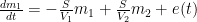
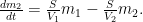
Those equations tell us that the carbon quantity 
![m_1(t) = \left[ \frac{V_1}{V_1+V_2}+\frac{V_2}{V_1+V_2} \exp\left(-\frac{V_1+V_2}{V_1V_2}St \right)\right] m_0 ,](https://s0.wp.com/latex.php?latex=m_1%28t%29+%3D+%5Cleft%5B+%5Cfrac%7BV_1%7D%7BV_1%2BV_2%7D%2B%5Cfrac%7BV_2%7D%7BV_1%2BV_2%7D+%5Cexp%5Cleft%28-%5Cfrac%7BV_1%2BV_2%7D%7BV_1V_2%7DSt+%5Cright%29%5Cright%5D+m_0+%2C+&bg=ffffff&fg=000&s=0&c=20201002)
which the substitutions 

Note that in the Fig. 2 system any constituent of the gas would be exchanged between vessels in accordance with the partial-pressure difference of that constituent alone, as if it were the only component the vessels contained. By thus constraining the flow from (and to) the first, atmosphere-representing vessel, this model supports the conclusion that the overall-carbon-dioxide quantity would, contrary to my previous argument, decay just as the excess, bomb-caused quantity of atmospheric carbon-14 did.

Could providing more than one sink enable us to escape that conclusion? Not necessarily. Consider the more-complex system that Fig. 3 depicts. Just as the system that my previous post described, this one can embody the TAR Bern-model parameters. As that post indicated, describing such a system requires a fourth-order linear differential equation. So that system does have more degrees of freedom in its initial conditions and can therefore exhibit a wider range of responses.
But it still constrains the flow among its four vessels linearly in accordance with partial pressures, just as the Fig. 2 system does. From complete equilibrium, therefore, its behavior for any constituent is the same as for any other constituent as well as for the contents as a whole. In other words, this model, too, seems to support the notion that the bomb-test results do indeed tell us how long excess carbon dioxide will remain if we stop taking advantage of fossil fuels.
In a sense, though, the models of Figs. 2 and 3 beg the question; they use the same uptake- and emissions-process-representing
So one question is how significant that difference is in the present context. I don’t have the answer, although my guess is, not very. But readers attempting to answer that question could do worse than start by referring to a previous WUWT post by Ferdinand Engelbeen.

Another way in which carbon-14 differs from the other two carbon isotopes is that it’s unstable. So, if the Fig. 3 model is adequate for carbon-12 or -13, a different model, which Fig. 4 depicts, would have to be used for carbon-14 if its radioactive decay is significant. That diagram differs from Fig. 3 in that it includes a flow 
To the extent that those different models produce different responses, using bomb-test data to predict the total carbon content’s behavior is problematic. But the Engelbeen post mentioned above seems to say that even deep-ocean residence times tend to be only a minor fraction of carbon-14’s half-life: this factor’s impact may be small.
A possibly more-significant factor is that the carbon cycle is undoubtedly non-linear, whereas the conclusions we tentatively drew from the models above depend greatly on their linearity. Before I reach that issue, though, I should point out an aspect of the Bern model that was not relevant to my previous post. The Bern equations I set forth in my last post were indeed linear. But that does not mean that their authors meant to say that the carbon cycle itself is. Although for the sake of simplicity I’ve discussed the models’ physical quantities as though they represented, e.g., the entire mass of carbon in a reservoir, their authors no doubt intended their (linear) models’ quantities to represent only the differences from some base, pre-industrial values. Presumably the purpose was to limit their range enough that the corresponding real-world behavior would approximate linearity.
But such linearization compromises the conclusions to which the models of Figs. 2 and 3 led us. A linear system is distinguished by the fact that its response to a composite stimulus always equals the sum of its individual responses to the stimulus’s various constituents; if the stimulus equals the sum of a step and a sine wave, for example, the system’s response to that stimulus will equal the sum of what its respective responses would have been to separate applications of the step and the sine wave. And this “superposition” property was central to drawing the conclusions we did from those models: the response to a large stimulus is proportionately the same as the response to a small one.

To appreciate this, consider Fig. 5, which depicts scaled values of the Fig. 2 model’s left-vessel total-carbon and carbon-14 contents. Initially, the system is at equilibrium, with zero outside emissions 


At time t = 5, a bolus of carbon-14 appears in the (atmosphere-representing) left vessel. Compared with the total carbon content, the added quantity is tiny, but it is large enough to double the small existing carbon-14 content. As the distance between the red dotted vertical lines shows, the resultant increase in carbon-14 content decays toward its new equilibrium value with a time constant of just about seven years. (I’ve assumed that the processes greatly favor the sink-representing right vessel—i.e., that its “volume” is much greater than the left vessel’s—so that the new equilibrium value is not much greater than the original.)
Now consider what happens at t = 45, when the left vessel’s total-carbon quantity suddenly increases. Although the two quantities are scaled to their respective initial values, this total-carbon increase is orders of magnitude greater than the t = 5 carbon-14 increase. Yet, as the black dotted vertical lines show, the decay of the left vessel’s total-carbon content proceeds just as fast proportionately as the much-smaller carbon-14 content did. As was observed above, this could tempt one to conclude that the carbon-14 decay we’ve observed in the real world tells us how fast the atmosphere would respond to our discontinuing fossil-fuel use.
![clip_image009[1]](http://wattsupwiththat.files.wordpress.com/2013/12/clip_image0091.png "clip_image009[1]")
But now consider what can happen if we relax the linearity assumption. Specifically, let’s say that the Fig. 2 model’s proportionality “constant”

In that plot, the red lines show that the carbon-14 decay occurs just as fast as in the previous plot, the carbon-14 content falling to exp(-1) above its new equilibrium value in around seven years. But the much-larger total-carbon increase brings the system into a lower-efficiency range, so that quantity subsides at a more-leisurely pace, taking over forty years. If such results are any indication, bomb-test results are a poor predictor of how long total-carbon content will settle.
Now permit me a digression in which I attempt to forestall pointless discussion of precisely what the quantities are that the graphs show. I believe the exposition is clearest if it is directed, as in Figs. 5 and 6, to ratios that carbon 14 and total carbon bear to their own initial values. But it appears customary to express the carbon-14 content instead in terms of its ratio to total carbon content. This means that, since total carbon has been increasing, the numbers commonly used in carbon-14 discussions could fall below the pre-bomb values, even though total carbon-14 has in fact increased.
For the sake of those to whom that issue looms large, I have attached Fig. 7 to illustrate how the values for carbon-14 itself could differ from those of its ratio to total carbon in a situation in which new (carbon-14-depleted) carbon is continually injected into the atmosphere.

But that’s a detail. More important is the issue that Fig. 6 raises.
Now, I “cooked” Fig. 6’s numbers to emphasize the point that nonlinearity can undermine conclusions based on linear models. Specifically, Fig. 6 depicts the results of making the flows proportional only to the fifth root of the carbon content.
But non-linearity must have some effect. How much? I don’t know. Together with the differences in behavior between carbon-14 and its stable siblings, though, it is among the considerations to take into account in assessing how informative the bomb-test data are.
As I warned at the top of the post, this post draws no conclusions from these considerations. But maybe the foregoing analysis will prompt knowledgeable readers’ comments that help narrow the issues.
Having studied archaeology, C14 is a radioactive isotope that is absorbed by all organic matter. Then it decays slowly. It has fluctuated over the years because of sun spot activity that deflect galactic sub atomic particles bombarding the earth. The same sub atomic particles also when they meld with water vapor molecules form clouds. I don’t know if it is correct, but before they banned atmospheric Atom and Hydrogen bombs the C.14 increased. We had terrible weather too lots of rain and cold temps in UK. That is why any carbon 14 dating usually gets a + or minus, and anything younger than say 2,000 is harder to date accurately and other dating methods have to be used.
OT but very funny and scary at the same time.
Stephen Colbert Tells David Keith Government is Already Spraying Us « GeoEngineering Exposed
Connecting CO2 sources/sinks in the manner shown here is analogous to the way an electrical engineer might connect multiple resistors and capacitors in a network without using any active elements (amplifiers or buffers). Because you can never achieve complex poles with this restriction, the resulting low-pass filters are not very useful (frequency characteristics are way too wimpy). We don’t do it that way.
This is NOT to suggest that the electrical equivalents could not be completely correct and very useful as models for CO2 migrations. The mathematics (that is – the physics) is very similar if not identical.
While NOT very useful for usual signal processing (analog filtering here) we do use these schemes for “envelope generators” for electronic music generation as I have recently reviewed at
http://electronotes.netfirms.com/EN210.pdf
[ In synthesizer design, “envelopes” are slowly-varying contours (way sub-audio) which are the parameters or controls for single tones (single notes).] My summary referenced here shows four approaches to solutions: the differential equation approach (eigen-analysis), but also the corresponding Laplace transform method, numerical simulation solutions, and finally a (gasp!) experiment. This comparison smorgasbord may be of interest here.
seeing as temperature over the history of the earth has changed dramatically, and the CO2 has changed with that temperature with a lag, then who cares. it seems rather obvious that the earth was & still is capable of absorbing CO2 in cooling conditions, so really it must be linear or something close to it or earth would not have survived as we know it.
Hopelessly over complicated. From Fig 5 and discussion, I question whether the writer understands the system we are talking about. 14C is effectively a tracer. There is a steady state level maintained by adding the same amount to the atmosphere each year from transmutation via cosmic ray interactions with nitrogen atoms in the atmosphere. The total amount of carbon is essentially unchanged. The atomic bombs did not increase the amount of CO2 in the atmosphere, but did almost double the tiny amount of 14C.
A basic reasonable assumption of a single turnover kinetics is the tracer leaves the reservoir and does not come back. 14C leaving the atmosphere can safely be assumed to not return in any significant fraction. Hence, when we see it leave, that is the off rate cleanly determined. Now when we have an equilibrium level, we can calculate the on rate as well. It doesn’t matter how complicated the reservoir system you create. The only part that matters is the off rate constant. We don’t know how the material partitions into other reservoirs, but that issue is beyond the scope of this experiment.
I showed previously [1] the math works out nicely, and essentially you can slice off the steady-state amount of 14C and look at the decay of the excess alone. The t1/2 is about 5 years. Even accounting for the increase in ppmv CO2 diluting the 14C from 1963 to 1993 and beyond, the t1/2 is still about 5 years (at least it was in my hands). Once you know the t1/2 is 5 years, a number of interesting calculations follow.
For one thing, it becomes pretty clear the increase in atmospheric CO2 cannot possibly be due to anthropogenic CO2. The CO2 quantity changes simply don’t match what humans have produced given the amount of CO2 we have produced each year from the late 1700s and how much would be left Y years after emission.
1) http://wattsupwiththat.com/2013/11/21/on-co2-residence-times-the-chicken-or-the-egg/#comment-1481426
Dear Joe,
By thus constraining the flow from (and to) the first, atmosphere-representing vessel, this model supports the conclusion that the overall-carbon-dioxide quantity would, contrary to my previous argument, decay just as the excess, bomb-caused quantity of atmospheric carbon-14 did.
The main problem with that model is that there is no lag included between the outflow (from the atmosphere in the deep oceans) and the inflow (from the deep oceans to the atmosphere). That makes that there is not only a huge difference in mass, but also a huge difference in concentrations of 14C.
What goes into the deep oceans is in direct ratio to the partial pressure difference of CO2 between atmosphere and ocean surface. What comes out is in direct ratio to the partial pressure difference of CO2 between ocean surface and atmosphere. That is the same for 12CO2 and 14CO2, with a small difference due to kinetics.
What goes into and comes from the deep oceans is thus directly related to their relative partial pressure differences.
For 12CO2 that is about 97% (in mass) * 99% (in concentration) that returns of what is going into the deep oceans, but for 14CO2, that is only 97% (in mass) * 45% (in concentration) at the time of the peak bomb test (1960):
http://www.ferdinand-engelbeen.be/klimaat/klim_img/14co2_distri_1960.jpg
The mass difference in this scheme is only at the inputs (to make the difference clear), but in reality it is equally distributed between deep ocean input and output to/from the atmosphere.
In pre-industrial times about 90% (45% of the bomb spike) of 14CO2 returned from the deep oceans for a ~1000 years lag, but that was about compensated by fresh production from cosmic rays.
Thus the 14CO2 decay is a mix of the mass spike decay (about equal to a 12CO2 mass spike decay) which depends of the atmospheric partial pressure and the “contamination” spike decay, which depends of the residence time.
That makes that the 14CO2 bomb spike decay rate of ~14 years is longer that the residence time, but shorter than the decay rate of a 12CO2 mass spike.
Something similar happens to the 13CO2 rate decay caused by the use of low-13C fossil fuels. If we look at the decrease of the 13C/12C ratio in the atmosphere, we see a decay rate which is only 1/3rd of what can be expected from the use of fossil fuels. That too is caused by the “thinning” from 13C-rich upwelling waters from the deep oceans. That can be used to estimate the deep ocean – atmosphere exchanges over a year:
http://www.ferdinand-engelbeen.be/klimaat/klim_img/deep_ocean_air_zero.jpg
or about 40 GtC/year in and out between atmosphere and deep oceans.
With that in mind, the residence times of a “human” CO2 spike can be estimated if we give a pulse of 13c-depleted CO2 of 100 GtC to the pre-industrial CO2 level of 580 Gtc:
http://www.ferdinand-engelbeen.be/klimaat/klim_img/fract_level_pulse.jpg
where FA is the fraction of “human” CO2 in the atmosphere, FL in surface waters, tCA total carbon in the atmosphere and nCA natural carbon in the atmosphere.
After ~60 years all low-13C from fossil fuels is replaced by “natural” CO2 from the deep oceans, while still 45% of the original total CO2 spike is present…
Hoser says:
December 11, 2013 at 11:32 pm
Your calcualtion is for the thinning of 14CO2 by the total CO2 turnover, which gives you the residence time (which is mainly temperature difference dependent), but that has nothing to do with the decay time for a mass pulse (which is mainly pressure difference dependent).
It is nothing humans can control anyway.
I’m grateful to Mr. Born for his detailed consideration of the CO2-lifetime question..The literature from Revelle onwards supports Hoser’s contention that the turnover time is 5-7 years: but that, as Mr. Engelbeen reminds us, is not the whole story. Dick Lindzen estimates that most CO2 molecules added to the atmosphere will have found their way out of it again in about 40 years. That is below the IPCC’s 50-200 years.
And the missing sink remains missing. Why is half of all the CO2 we emit disappearing instantaneously from the atmosphere? I’d be most grateful if wiser heads than mine were able to explain that.
Ferdinand Engelbeen says:
December 12, 2013 at 12:27 am
Hoser says:
December 11, 2013 at 11:32 pm
Your calcualtion is for the thinning of 14CO2 by the total CO2 turnover, which gives you the residence time (which is mainly temperature difference dependent), but that has nothing to do with the decay time for a mass pulse (which is mainly pressure difference dependent).
NO NO NO NO NO NO NO NOOOOOO! (adopts facial expression of The scream by Munch)
Ferdninand we all respect your erudition in regard to atmospheric CO2 but I fully agree here with Hoser that all this discussion is completely missing what a radio tracer measurement really is. And vastly over-complicating the discussion as a result.
A radiotracer measures a single removal term. PERIOD. A pulse of CO2 enters the atmosphere different from the other CO2 due to 14C. So it can be tracked in exclusion of any other CO2.
It is COMPLETELY IRRELEVANT all the other cycling and dilution and dynamics, pressure, temperature etc. of CO2 that are going on, the 14 tracer simply tells us the removal term for CO2. That is the whole point of a radiotracer measurement.
From the bomb test data we know that:
CO2 removal half life = 5 years
CO2 residence time = half life / ln2 = 5 / 0.693 = 7.7 years
That is the WHAT. Everything else is the WHY.
Cl4 can not be absorbed once the organism dies, or is buried. So that is how they can calculate by the amount of half life remaining how old the organism is. Anything organic including bones, trees etc., that have been unearthed in an archaeological site. I can’t see the problem really, we are bombarded all the time by galactic sub atomic particles. When sun pot activity is large then we don’t receive as much. Inactive and we receive a lot, including more clouds.
As a layman reading this it seems to over complicate the issue but you will see my ignorance shine through from my comment ! C14 as a tracer should provide a reasonable means of tracking the removal or sequestration rate of CO2.
We know from NASA that higher levels of CO2 have resulted in an increase of ~15% in vegetative matter globally which has ‘captured’ and removed CO2, although I don’t know if any calculations or studies show the likely amount of CO2 by weight and percentage that is. I assume there must be and that forward projections of increased rates of capture in higher CO2 levels are there somewhere. As an aside – I wonder if the increase in tree growth and number of leaves increases the release rate of volatile organics which in turn serve to increase forest related cloud formation and increased rainfall – or maybe with less water requirement (elevated CO2 and fewer stoma) they respond by producing less VO ?
Bacteria (some anyway) capture carbon and there is a strong likelihood that the populations of these may explode or implode depending on ambient CO2 levels which suit them best, again I don’t know if this has been studied or evaluated although it potentially may have very dramatic effects on the rate of carbon sequestration. Ditto bacteria which emit CO2.
I cannot see how the ‘bath tub’ simile has any value at all without including a means to show some form of active sequestration within the first bath tub. As you can see I am filled with curious ignorance.
Joe Born: “The observed decay of bomb-generated atmospheric-carbon-14 concentration does not tell us how fast elevated atmospheric carbon-dioxide levels would subside if we discontinued the elevated emissions that are causing them.”
Yes, but as Lubos Motl has pointed out, we can easily calculate this rate without bothering with 14C.
Lubos Motl says:
November 22, 2013 at 1:42 am
“It’s trivial to see that the residence time of CO2 is of order 30 years or longer. We emit 4 ppm worth of CO2 a year; the CO2 concentration increases by 2 ppm per year. So it’s clear that the “excess uptake” (which is natural and depends on the elevated CO2 relatively to the equilibrium) is also 2 ppm pear year. The excess CO2 above the equilibrium value for our temperature- which is still around 280 ppm – is about 120 ppm so one needs about 30 years to halve the excess CO2 and 50 years to divide it by e.”
Residence time τ can been defined (Barth, 1952, quoted by Henderson, 1982§) as τ = A/(dA/dt), where A is the amount of a substance dissolved or contained in a reservoir and dA/dt is the rate of efflux of that substance from the reservoir. In the case here considered the ‘substance’ can be considered as the excess atmospheric CO2 above the equilibrium value for today’s temperatures (around 280ppm). So if today’s CO2 concentration is about 400ppm, then A = 400 – 280 = 120ppm.
If (as Lubos states) the equivalent of 4ppm excess (i.e. anthropogenic) CO2 is being emitted to the atmosphere annually, while the concentration in the atmosphere is increasing by 2ppm/year, then dA/dt = 2ppm/year and τ (the residence time in the atmosphere of the excess CO2) is 120/2 years, so 60 years. Of course that assumes that anthropogenic omissions cease now, which they won’t…but any talk of residence time being less than 10 years is unrealistic.
§ Henderson, P. 1982. Inorganic geochemistry. p. 287.
Ferdinand Engelbeen:
Thank you very much for the response. I’m going to have to get some coffee in me before I digest it all, but it seems to me that your third graph is actually your answer to the ultimate question. I think I’ll have questions about how you get there, but I won’t impose upon you until I’ve prayed and fasted a bit over what you’ve already said. Except for one question now:
I didn’t quite understand that passage:
“For 12CO2 that is about 97% (in mass) * 99% (in concentration) that returns of what is going into the deep oceans, but for 14CO2, that is only 97% (in mass) * 45% (in concentration) at the time of the peak bomb test (1960).”
. The 45% figure, I take it, comes from the fact that the deep oceans absorbed half the bomb-peak concentration and so are returning that, minus a 10% loss from beta decay: 0.5 * (1.0 – 0.1) = 0.45. So the 14C02 partial pressure from the deep oceans is 45% that of the bomb-peak atmosphere’s? And what is the “97% (mass)” by which you multiply the concentrations?
There are other ways of getting an estimate on the withdrawal rate of CO2.
http://wattsupwiththat.com/2008/04/06/co2-monthly-mean-at-mauna-loa-leveling-off/
Has graphs of the CO2 measured in Hawaii.
You can see that at particular times of the year, there are drops. That drop shows the rate at which C02 can be withdrawn by the system. It’s large.
There are other examples with temperature lags in the system. Now if only we could experiment with the earth we could find out those lags. Right? Hmmm, how about turning the sun off for 12 hours and seeing how quickly things cool. Small drops in temperature mean large lags. Large drops small lags. Low an behold the night day temperature difference shows very small lags in the system to changes in forcings.
Do we have data on the response to 14C bomb spike of carbon reservoirs other than the atmosphere?
phlogiston says:
December 12, 2013 at 12:53 am
A radiotracer measures a single removal term. PERIOD. A pulse of CO2 enters the atmosphere different from the other CO2 due to 14C. So it can be tracked in exclusion of any other CO2.
In this case, the radiotracer meausures not only the removal term (as mass), but also the “thinning” of the concentration, because what returns from the deep is only halve the concentration (at the height of the bomb spike) of what goes into the deep oceans. Two distinct removal rates without much connection with each other.
The decay rate of a 12CO2 pulse only depends of the mass balance between ins and outs, the decay rate of a 14CO2 pulse mainly depends of the concentration balance and hardly the (total) mass balance between ins and outs.
An important problem is emerging. The Kyoto Annexe II countries are gearing up to impose financial penalties on Annexe I (‘developed’) countries proportional to their cumulative CO2 emissions. But if the half-life of CO2 in the air is (say)20 years, instead of the thousands that some claim, then the ‘legacy’ CO2 of Annexe I countries is much lower. Indeed, as China now emits more COS then the US, then it will soon have a larger legacy concentration. China is of course an Annexe II country, and determined to remain so. But their share of the COs now in the atmosphere is rapidly heading into second place, given that mush of the US CO2 was emitted long ago.
studying the decay times for C14 does not help calculate the CO2 residence time. C12 is preferentially used by plants in photosynthesis as opposed to other isotopes. They remain in the atmosphere so would give a false reading.
I loved your discussion but it caused a flashback to my nightmarish college calculus classes.
Joe Born says:
December 12, 2013 at 1:49 am
Some background:
The 1950-1960 bomb spike almost doubled the existing 14CO2 “background” levels. If we take the maximum bomb spike level of 1960 as 100%, the pre-industrial 14CO2 level in the atmosphere thus was 50% of the bomb spike.
– in pre-industrial times there was a balance between decay and production of 14CO2:
http://www.ferdinand-engelbeen.be/klimaat/klim_img/14co2_distri_1850.jpg
Some 14CO2 is distributed and removed via vegetation and the ocean surface, but the bulk is removed by the deep oceans: 50% bomb spike level goes into the deep oceans, 45% comes out after ~1000 years, that is 90% coming back, the difference is the radioactive decay of 14CO2 over that time span + mixing in of older 14CO2 free carbon from deep sources (CH4, carbonate dissolution).
The continuous 14CO2 production in the atmosphere from cosmic rays compensated for the losses.
– since ~1850 there is an increase of 14CO2-free fossil emissions, which had some impact on the 14C/12C ratio, which made it necessary to adjust the radiocarbon dating tables.
– about 1960, at the height of the 14CO2 bomb spike, there was already a measurable increase of (mainly) 12CO2 in the atmosphere:
http://www.ferdinand-engelbeen.be/klimaat/klim_img/14co2_distri_1960.jpg
That caused an imbalance between atmosphere and deep oceans where inputs and outputs aren’t equal anymore. While that mainly influenced the bulk of CO2 (which is ~99% 12CO2), that also influenced the 14CO2 spike to a lesser extent: 40.5 GtC out of the atmosphere into the deep oceans, 39.5 GtC into the atmosphere, caused by the extra pressure from the 100 GtC increase of CO2 in the atmosphere. That is for 100% CO2 out into the deep, 97.5% is coming back from the deep oceans. The difference in 12CO2 concentration between ins and outs (both ~99%) is negligible.
Not so for 13CO2 and 14CO2.
From the 100% 14CO2 spike going into the deep (1960), 97.5% (as mass) * 45% (as concentration) is coming back, that is only 42.8% is coming back from the deep oceans.
The difference between a 12CO2 spike and a 14CO2 spike is caused by the long delay between what goes into the oceans and what comes out, which makes that the 14CO2 (and 13CO2) input is effectively decoupled from the output, while that is hardly the case for 12CO2.
For the year 2000, things changed for both 14CO2 and 12CO2:
http://www.ferdinand-engelbeen.be/klimaat/klim_img/14co2_distri_2000.jpg
Berényi Péter says:
December 12, 2013 at 1:53 am
Do we have data on the response to 14C bomb spike of carbon reservoirs other than the atmosphere?
Here an interesting reference for the 14CO2 distribution in general and specific for the bomb spike:
http://shadow.eas.gatech.edu/~kcobb/isochem/lectures/lecture10_14C.ppt
Isn’t open science fascinating?
“….. if we stop taking advantage of fossil fuels.”
Damn! I like that term.
That’s exactly how it should be looked at and expressed every time – fossil fuel is not pollution…it’s an advantage.
cn
Ahhh. My first day of pharmacology. This is a multi-compartment model — atmosphere, oceans, plants, soil etc.
A multi-compartment model is a type of mathematical model used for describing the way materials or energies are transmitted among the compartments of a system. Each compartment is assumed to be a homogenous entity within which the entities being modelled are equivalent. For instance, in a pharmacokinetic model, the compartments may represent different sections of a body within which the concentration of a drug is assumed to be uniformly equal.
Hence a multi-compartment model is a lumped parameters model.
Multi-compartment models are used in many fields including pharmacokinetics, epidemiology, biomedicine, systems theory, complexity theory, engineering, physics, information science and social science. The circuits systems can be viewed as a multi-compartment model as well.
http://en.wikipedia.org/wiki/Multi-compartment_model
I have seen the point made hundreds of times that the residence time of an average molecule is different than the time for a pulse to decay back to equilibrium. Usually this point is made in pedantic fashion, as if it were a tiresome chore to explain such a simple point to such simpletons. But I still don’t get it. Are the molecules in the pulse exempt from the processes giving rise to the properties of the residence time of average molecules? Are they not average molecules? How so? What qualifies a molecule, or group of molecules, to be treated as part of a slug or pulse on the one hand that is governed by pulse decay rules or merely part of the background sources of emissions governed by residence time of average molecule rules? How do it know? Where human emissions are a single digit percentage of natural emissions, which source is the slug? What is the threshold at which or the rules by which emissions from one or the other, human or natural, transition from being subject to average molecule processes to slug molecule processes? How do it know?
Ferdinand Engelbeen: “40.5 GtC out of the atmosphere into the deep oceans, 39.5 GtC into the atmosphere, caused by the extra pressure from the 100 GtC increase of CO2 in the atmosphere. That is for 100% CO2 out into the deep, 97.5% is coming back from the deep oceans.”
Thanks a lot for that response; it answers my question nicely.
If I can again abuse your patience, what are K and k in your diagrams? I couldn’t readily find the accompanying text on your site.
Ferdinand Englebeen: “From the 100% 14CO2 spike going into the deep (1960), 97.5% (as mass) * 45% (as concentration) is coming back, that is only 42.8% is coming back from the deep oceans.” Is this the loss of that spike since 1960 or is it a suggestion that the kinetic difference between 14C and 12C is that large? I couldn’t quickly find kinetic differences for carbon isotopes but would be surprised if they are that large. I’d also expect the kinetic differences to be process dependent.
Bernie Hutchins “This is NOT to suggest that the electrical equivalents could not be completely correct and very useful as models for CO2 migrations. The mathematics (that is – the physics) is very similar if not identical.”
For the linear models above, RC-circuit mathematics is indeed identical. But using a signed quantity (charge) to represent an unsigned quantity (mass) can lead to some conceptual confusion. Although the left vessel is connected in series between the source and the right vessel, for example, the analog’s current source would have to be wired in parallel with the capacitor representing the left vessel and with the RC-series combination representing the right vessel and its flow restriction.
I assume all the discussion of CO2 mass balance is based on the assumption that the CO2 distribution in the atmosphere is homogeneous and can be represented by one measuring location. Other things, liquid or gas, require relatively great amounts of energy to get homogeneous mixtures at much lower volumes. Is the atmospheric CO2 that homogeneous and if not, how much does that affect these estimates?
Bob Greene: “Is the atmospheric CO2 that homogeneous and if not, how much does that affect these estimates?”
Someone has probably already answered this question somewhere, but I haven’t found it yet myself. I’ve wondered whether the “missing sink” may be a reflection of greatly enhanced uptake at areas of locally intense near-power-plant (or -highway) concentrations not reflected in the more-general CO2 numbers we see–uptake that is not offset substantially by locally enhanced natural emissions.
No doubt a naive notion that has already been laid to rest elsewhere, but it’s one of which I haven’t yet been disabused.
Quinn the Eskimo says:
December 12, 2013 at 4:07 am
I have seen the point made hundreds of times that the residence time of an average molecule is different than the time for a pulse to decay back to equilibrium.
I know, this seems to be one of the most difficult points to be explained…
The simplest way is to describe it as the difference between the turnover of capital (thus goods) in a factory and the gain or loss that that capital makes (over a year).
The turnover gives how much times a capital is going through the factory: from the purchase of raw materials to the sales of the endproduct.
The yield of the factory is what is gained or lost of its capital after the turnover(s).
Both are about the same money, but they are largely independent of each other: you can double the turnover, but that may or may not increase the gain, because you have to pay higher wages for overtime, or you may get from a loss to a gain…
The same for 14CO2 vs. 12CO2:
With the 14CO2 bomb spike, you are mostly measuring the turnover of CO2 through the atmosphere, without influencing the mass (total capital).
With a 12CO2 spike, you are increasing the total mass (capital), whithout influencing the turnover that much: the turnover will be somewhat diluted (more in the atmosphere, about the same througput).
The decay rate of an excess mass of 12CO2 depends of how fast the deep oceans (less for other reservoirs) take an extra mass of CO2 away from the atmosphere (partial pressure difference related), while the decay rate of an excess concentration of 14CO2 depends of the turnover (which is temperature difference related, mostly between equator and poles)…
Monckton of Brenchley says:
December 12, 2013 at 12:51 am
Why is half of all the CO2 we emit disappearing instantaneously from the atmosphere?
============
This does appear to be the nub of the problem. Why does this number remain at 1/2 of human emissions, rather than a fraction of cumulative CO2 excess?
If we consider the bathtub model, then the amount flowing out remains at 1/2 the amount flowing in, regardless of the height of water in the tub. Which makes no sense. The amount flowing out should vary as the height of water in the tub, not as the amount flowing in.
Which argues that the bathtub model does not describe CO2 reality.
Joe Born says:
December 12, 2013 at 4:16 am
If I can again abuse your patience, what are K and k in your diagrams? I couldn’t readily find the accompanying text on your site.
You are welcome…
K and k should all be k and are the rate constants for all transfers, where I should switch the +’s and -‘s, as normally one looks at the atmosphere as starting and end place…
Still to be worked out, as good as the whole page I need to devote to the explanation of all these diagrams and a lot more…
The methane residency time is also likely much lower than currently believed. As we discover more and more sources, we must realize that there more sinks or that sinks respond to emissions to keep methane levels from growing much.
ferd berple says:
December 12, 2013 at 4:47 am
This does appear to be the nub of the problem. Why does this number remain at 1/2 of human emissions, rather than a fraction of cumulative CO2 excess?
In fact it is pure coincidence: human emissions increased slightly quadratic over time, which gives a slightly quadratic increase of the residuals in the atmosphere (= pressure) and which causes a slightly quadratic increase in sink rate. The result is an astonishing fixed ratio between emissions and increase in the atmosphere (the “airborne fraction”):
http://www.ferdinand-engelbeen.be/klimaat/klim_img/temp_co2_acc_1960_cur.jpg
or in ratio since 1900:
http://www.ferdinand-engelbeen.be/klimaat/klim_img/acc_co2_1900_cur.jpg
or since 1960:
http://www.ferdinand-engelbeen.be/klimaat/klim_img/acc_co2_1960_cur.jpg
where the South Pole (SPO) lags the Mauna Loa (MLO) data.
If the human emissions would stay the same, the “airborne fraction” would decrease and CO2 levels would go assymptotically to a new steady state equilibrium CO2 level…
Hoser says:
December 11, 2013 at 11:32 pm
Hopelessly over complicated.
—————————
Indeed. All this analysis of 1 part of 20,000 parts of the atmosphere changing from “something” to CO2. A change of .005%, while the other 99.995% purportedly has been expected to remain stable and have influence. Oh the effort that has been spent on solving a puzzle that is simply a figment of someone’s overactive imagination.
Bob Greene says:
December 12, 2013 at 4:29 am
I assume all the discussion of CO2 mass balance is based on the assumption that the CO2 distribution in the atmosphere is homogeneous and can be represented by one measuring location.
For most of the atmosphere, the CO2 levels are within +/- 2% of full scale, despite that some 20% of all CO2 in the atmosphere is exchanged with CO2 of other reservoirs each year. Seems to be quite nicely and fast mixed. There are lags between near-ground and height and between the NH and the SH. The largest differences are in the first few hundred meters over land, where the largest/fastest sources and sinks are at work.
But have a look at what different stations find:
http://www.esrl.noaa.gov/gmd/dv/iadv/
Thus while there are huge CO2 level differences around vegetation (day/night difference of several hundred ppmv!), that doesn’t exist for the air over the oceans, where the 14C/12C decay rates have the highest difference in decay rate…
It also means there’s a good bit of fossil carbon in the atmosphere from natural sources.
I take no joy in this, but the fallacies are so deep that it warrants no less than a full fisking of Ferdinand:
” 50% bomb spike level goes into the deep oceans, 45% comes out after ~1000 years,”
Maxwell called and said he wanted his demon back. Putting aside gedankens of nonsense, it is wholly irrelevant to the topic at hand: The bomb spikes that happened ~50 years ago. Perhaps the argument can be salvaged with clarity, and perhaps it would be worthwhile to do so if we were discussing some other subject.
“That caused an imbalance between atmosphere and deep oceans where inputs and outputs aren’t equal anymore. ”
The ice core records show that ‘aren’t equal anymore‘ places ‘anymore’ prior to the ice core records themselves. There has never been a proper equality. This is confused and nonresponsive at best, and an attempt at sophistical obfuscation at worst.
“40.5 GtC out of the atmosphere into the deep oceans, 39.5 GtC into the atmosphere, caused by the extra pressure from the 100 GtC increase of CO2 in the atmosphere. ”
Based on what measurements? This is first-order circular nonsense. As it presumes the rates to exist — without any measurements taken — on the basis of global average temperatures as compared to salinity and etc. The 14CO2 discussion is precisely about discarding this vulgar fallacy and making use of actual observations — for good or ill. One cannot ‘prove’ your conclusion by assuming it as a premise. Again, a thoroughly confused point at best, or a sophistry at worst.
“The difference in 12CO2 concentration between ins and outs (both ~99%) is negligible.
Not so for 13CO2 and 14CO2.”
With respect to 14C there is the issue of the radioactive decay that would occur with or without Maxwell’s lesser demon of oceanic circulation. But it was already stated in the same post that: in pre-industrial times there was a balance between decay and production of 14CO2:
Whatever the case may be with radioactive decay is meaningless here. For there was, and ppresumptively is, the same process extant. To the degree there is not that can be haggled over. But tagging a herd of Carbon Dioxide with radioactive tracers isn’t going to upset this long running process that has been stated to be balanced. Again, deep confusion or sophistry.
With respect to isotopic fixation in organisms, it only needs noted that 12C is preferred. So we would see
more 12C sequestered — versus exchanged — than 13C and 14C. That is, the decay curve in the bomb spike represents an upper bound on time for the process in question. But this has precisely nothing to do with the thrust of the ‘ins and outs’ statement or the statements about 14C and CH4.
“The difference between a 12CO2 spike and a 14CO2 spike is caused by the long delay between what goes into the oceans and what comes out, which makes that the 14CO2 (and 13CO2) input is effectively decoupled from the output, while that is hardly the case for 12CO2.”
This is again an instance of Maxwell’s demon. But the difference is between a bolus of CO2 — of any and all isotopes — and radioactively tagging a set of the existing bolus. And to be sure, the idea that there is an increasing ppm of atmospheric CO2 is the entire argument of AGW. That there is a constant excess above equilibrium injected into the atmospheric reservoir. So yes, they are different creatures. One is a bolus without remark, as a pure gedanken, and the other is the actual physical process the gedanken represents — just with extra tagging of the molecules. No more nor less.
So the 13 and 14 CO2 are only decoupled from the output in the same manner that the pedestrian evil of 12CO2 is decoupled. Which is: They aren’t. Perhaps in the purely fictional land of idealized models that have no application outside of validation with measurement. But, once more, this entire discussion is about the rare sighting of a wild observation. A practically mythical beast long thought to be extinct.
Lastly, and out of order from the rest: “From the 100% 14CO2 spike going into the deep (1960), 97.5% (as mass) * 45% (as concentration) is coming back, that is only 42.8% is coming back from the deep oceans.”
Sadly, this one is full of confusion and/or sophistry again. There is again the circular argument based on the models proving the models. There is again, the idea that theory trumps measurement. There is again the special pleading about the deep oceans. The only relevant part to this is that the exchange does matter. And is the entire point behind looking at the bomb test curve in the first place. As given the increasing ppm of CO2, it is not a question that more CO2 is entering the atmosphere than leaving it. And the 14CO2 decay curve gives us an idea of the net flow on the basis of that decay.
There is a lot of heel digging on this issue for no good reason, as the math is entirely straight forward for it. We know the 14CO2 production rate, the (Bomb14)CO2 decay rate, and the historical levels — and so the partial pressure of the atmospheric reservoir of 14CO2; if you’re into bathtub models. Everything is right there to gain the answer.
It is, of course, wholly optional. As we can also get the same sanity check on CO2 cycling by looking at the unsmoothed data from Mauna Loa and other measuring sites. As every summer season the CO2 levels fair plummet. To the degree we add man’s culpability, and have a good measure of how much CO2 that dire beast is putting in the atmostphere, then the rest can be figured out independently from there as well.
That’s two — count them, two — independent sources of actual measurement that can be used to ground the entire discussion in science. The utter allergy to approaching the simple math for either of these is wholly incomprehensible. But Ferdinand deserves a round of applause for suffocating his straw man under a heap of errors.
Ferdinand Engelbeen says:
December 12, 2013 at 5:07 am
In fact it is pure coincidence: …. The result is an astonishing fixed ratio between emissions and increase in the atmosphere
==============
As I explained to the police, it was pure co-incidence my gun was smoking when the victim dropped dead.
What if we make the other assumption, that it is not co-incidence? Does this have implications for the choice of model? If the ratio is not due to co-incidence, but rather the nature of the system, how would this change the model?
phlogiston says:
December 12, 2013 at 12:53 am
It is COMPLETELY IRRELEVANT all the other cycling and dilution and dynamics, pressure, temperature etc. of CO2 that are going on, the 14 tracer simply tells us the removal term for CO2. That is the whole point of a radiotracer measurement.
———————————————————
Amen to that, and no amount of mental masturbation can change it.
This math(s) is virtually identical to that used by pharmacologists/pharmacokineticists for calculating drug dosage in animal models and human studies and treatment. They get it wrong, people die.
Typically, the drug is considered to be, for all intents and purposes, gone at six half-lives, explaining approximately, by analogy, Lindzen’s number (40 years) mentioned in Lord Monckton’s post above.
What reemerges from the sinks, and why is a separate discussion from this. This is the experimentally observed removal term which anyone can see from eyeballing the bomb data is a half-life of 5 or so years.
Ferdinand,
You have the patience of a saint, but are you really making progress? There are none so blind as those who refuse to see.
An elegant mathematical exploration of the travels of our most talked about substance. However indeed,
“Maybe various sinks saturate or become less efficient with increased concentration.”
So far, only the gas guys have responded. CO2 is also a complex chemical, forming carbonic acid in the atmosphere with rain and in its solution into the ocean. Once in the water the acid dissociates into three species:
CO2 +;H2O => H2CO3 => H^+ + HCO3^- => 2nd H^+ + CO3^-2
Now in seawater we have Ca^++ (and other cations which reacts which forms both inorganic limestone precipitate and biologically produced CaCO3 in shells (possibly through the bicarbonate stage), etc. This is sequestered CO2. Also, probably C14 is probably taken up by algae, plankton and the like, similar to the absorption by land plants. Go for the model where the sinks INCREASE their intake by sequestration.
ferd berple says:
December 12, 2013 at 5:43 am
If the ratio is not due to co-incidence, but rather the nature of the system, how would this change the model?
The “model” in this case is the most simple form of reaction: the sink rate of CO2 is directly proportional to the increase in the atmosphere above the (temperature controlled) equilibrium…
Oh my! I remember the hours spent learning to produce qualitatively effective curves of individual isotope activities in a closely empirically engineered system, a nuclear reactor. To attempt the same in an open system is amazing and beyond my ken. I knew that my curves were merely CARTOONS of reality.
Gary Pearse says:
December 12, 2013 at 5:47 am
Go for the model where the sinks INCREASE their intake by sequestration.
==========
In such a bathtub, the drain gets bigger as you increase the input flow. The output is no longer coupled to the height of the bath, rather to the inflow rate.
So, in such a model we have a reverse of the co-incidence proposed above. It is the cumulative excess that is the co-incidence, and the inflow rate that is the determining factor in the outflow.
Such a model may in fact be more likely than the standard bathtub model because the water in a bathtub is not in short supply. But in nature there is ample evidence that CO2 is barely above the minimum required by plants to maintain photosynthesis. As we add CO2 the drain (life) is increasing in size.
In this case it would not be partial pressure that is steering the good ship CO2, rather it is life.
Your figure 4 is essentially right from a simplest box model approach; with V1 atmosphere, V2 terrestrial biomass, V3 the ocean SURFACE and V4 the depths.
Please do not use the word SINK when you mean reservoir, a sink in local or process that is infinite, a kinetic black hole where there is, on the time scale analyzed, zero back rate. In your figure 4 you include a true sink out of V4, the mineralization of carbon.
Now mechanistically we know that the atmosphere. V1, can ‘talk’ to the ocean surface, V3, but cannot ‘talk’ to the deep ocean, V4.
Let us take what we know we know:-
The disappearance of 14CO2 from the atmosphere is first order all the way from the 70’s with a t1/2 of approx 12.5 years.
The disappearance of 14CO2 from the atmosphere has a projected endpoint very near to the pre-1945 levels.
What we can logically conclude from these two observations.
As atmospheric 14CO2 is being diluted into a reservoir that >40 times bigger, and we know the approximate sizes of all the reservoir’s, we can conclude that the only reservoir big enough to dilute 14CO2 is the deep ocean.
We know that atmospheric 14CO2 MUST interact with the surface layer, before it can interrogate the depths.
The rate of 14CO2 in V1, into V3 and then into V4 has an overall t1/2 of 12.5 years, which is the rate of V1 to V3 or V3 to V4.
As some estimates of residency time of atmospheric CO2 suggest half-lives of 4-7 years, it follows that the simplest mechanism is that
V1 to V3 has a half-life of 6 years, a first order rate of 0.11 y-1
V3 to V4 has a half-life of 12.5 years, a first order rate of 0.055 y-1
The sink rate, mineralization, should match the rate that volcanic CO2 is added to the system, over geological time.
Over geological time, 800,000 years, the volcanic injection of CO2 into the atmosphere is not stable, indicated by ice-core sulphate levels.
Over geological time, 800,000 years, the levels of atmospheric CO2 are pretty stable (230-290 ppm), indicated by ice-core CO2 levels.
It follows that the sink rate is dynamic with respect to atmospheric CO2, and when CO2 levels are low, atmospheric CO2 is not mineralized, but when large amounts of CO2 is injected into the atmospheric by large scale volcanic activity, atmospheric CO2 levels fall quickly back to the ‘normal’ steady state levels.
Typically, chemical processes do not have such concentration threshold effects, but crucially, biological processes like carbon fixation do.
We can therefore speculate that the mineralization sink rate is governed by biological, and not chemical, activity and kinetics.
PS Carbon dioxide molecules do no know what they are doing in a reservoir and do not calculate if it is the thermodynamical appropriate thing to do to move from one reservoir to another, they do not know what a delta[CO2] is and don’t care a damn about entropy; they just move, without thought, plan or knowledge of the system they are in.
Thinking back many years to my chemical engineering phase, it seems to me this process may bear some resemblance to the concepts I studied and applied then, the ‘purge stream’, for example.
So this document might throw some light on the subject (or not, of course!)
http://che31.weebly.com/uploads/3/7/4/3/3743741/lect12-recycle-bypass-purge.pdf
Just a thought…
Jquip says:
December 12, 2013 at 5:40 am
Putting aside gedankens of nonsense, it is wholly irrelevant to the topic at hand: The bomb spikes that happened ~50 years ago.
Jquip, what goes into the deep oceans is the isotopic composition of today (minus some fractionation), what comes out of the deep oceans is the isotopic composition of ~1000 years ago (minus some fractionation and some radioactive dexay). That is irrelevant for what happens with a 12CO2 mass spike, but that is highly relevant for the 14CO2 concentration spike.
That gives completely different decay rates for a 12CO2 spike, which is only mass/pressure dependent and for a 14CO2 spike which is (total CO2) mass dependent and concentration dependent. Which makes that the 14CO2 concentration decay is much faster than for a 12CO2 excess mass decay.
The ice core records show that ‘aren’t equal anymore‘ places ‘anymore’ prior to the ice core records themselves. There has never been a proper equality.
The ice core records show a thight ratio between CO2 levels and T levels of ~8 ppmv/K ranging over periods from a few decades (MWP-LIA) to multi-millennia. The rate of change was at maximum 0.8 K for 6 ppmv over 5o years (MWP-LIA) or 0.12 ppmv/yr. The current rate of change in the past 50 years is near 20 times faster for an increase of 0.6 K and increasing even in the past 17 years without T increase. Just by coincidence, while humans are emitting twice the increase of CO2 in the atmosphere?
As it presumes the rates to exist — without any measurements taken —
The 40 GtC/yr exchange rate is my own estimate based on the difference between the theoretical decrease of the 13C/12C ratio in the atmosphere and the observed decrease. Thus based on measurements:
http://www.ferdinand-engelbeen.be/klimaat/klim_img/deep_ocean_air_zero.jpg
It may be 40 GtC/yr or more or less. That is important for the decay rate of the 14CO2 concentration spike, but is completely unimportant for a 12CO2 mass spike: the latter only decays from a differencein mass flow between inputs and outputs, not from a difference in concentration between inputs and outputs, neither from the absolute height of the carbon exchange.
Any uptake of CO2 by the oceans (and reverse) is directly proportional to the partial pressure difference between atmosphere and oceans. If the levels in the atmosphere increase, more is going into the ocean sinks and less is coming out of the upwelling sites. It is the unbalance between the uptake and release that makes that a part of the excess CO2 (currently ~2 ppmv for an excess level of 110 ppmv) is absorbed by the oceans and other reservoirs. If there was no unbalance, then any 12CO2 spike would remain forever in the atmosphere, whatever the 14CO2 spike decay. But there is hardly any connection between the height of the throughput (the 40 GtC/yr) and the unbalance.
But, once more, this entire discussion is about the rare sighting of a wild observation.
Except that the observation does observe the exchange rate of 14CO2 and 12CO2 between the different reservoirs alike, but doesn’t show the decay rate of an excess amount of CO2 in the atmosphere, as that is independent of the exchange rate…
There is again the circular argument based on the models proving the models.
Nothing to do with models: what goes into the deep is the measured isotopic composition of the day. What comes out is the measured composition of ~1000 years ago minus the radioactive decay. 14CO2: 100% in, 45% out; 12CO2: 99% in, 99% out (1960) * the ins/outs as total mass.
hogwash….it’s the equivalent of the residence time of water in a sponge
It doesn’t matter how ‘high’ CO2 levels go…it’s not sustained
If it’s not replaced it still goes to zero
DocMartyn: “Now mechanistically we know that the atmosphere. V1, can ‘talk’ to the ocean surface, V3, but cannot ‘talk’ to the deep ocean, V4.”
Of course, deep-ocean water does have to come to the surface for interchange with the atmosphere. But looking at Mr. Engelbeen’s diagrams made me wonder whether the thermohaline circulation might result in behavior that mathematically is better matched by a model like the one you commented on in my last post.
I have no idea. But my (very brief) attempt to get the model above to match the Bern TAR behavior resulted in V values that didn’t immediately appeal to my intuition.
Michael, that is just plain nuts, but you don’t know that.
It’s too bad people like yourself NEVER got out more and experienced the REAL world, like a stint in the air force or the flying in the Navy, THEN you would not look so gullible and stupid posting material like this and making ridiculous claims, and this is sad, because, you *could* have something to contribute if and only if you were rational.
Sadly, you are not, rather, you appear to be ‘permanently wired’ for con spiracies not being able to work out the logistics (the material, the machines, and the men to carry it out) for the assertions (the ‘act’ of large scale or even small scale geo engineering) WHICH would show they are both highly improbable AND impractical.
Again, in your isolation, not associating with REAL people in the world (via church or social organizations or professional organizations; simply reading ZH does not count!)
Get a job, volunteer to work with the Red Cross or join some other civic organization and get some EXPOSURE to the rel world before its too late! Recovery will NOT become easier as you age … you don’t want to be known as a ‘raving nutter’ in your 60’s!!!!
.
DocMartyn says:
December 12, 2013 at 6:42 am
The connection between atmosphere and deep oceans is rather direct: sinks are going straight into the deep oceans and upwelling is also direct. Both are 5% of the total surface area of the oceans. For the rest of the oceans there is little connection between ocean surface and deep oceans, not in migration, not in temperature. There are exchanges by biolife, but as biolife in the oceans is not CO2 starved contrary to land plants, more CO2 in the oceans has no influence on biolife.
Therefore one can better see V3 and V4 as both directly connected to V1, which makes the calculations easier to follow with each their own exchange rates.
PS, CO2 movements between the oceans and the atmosphere are directly in ratio to the pCO2 difference between both: pCO2 is a measure for the number of CO2 molecules moving out of the water – for pCO2(aq) – or into the water – for pCO2(atm) -.
If pCO2(aq) = pCO2(atm) the same number of CO2 molecules get out as get in over the same time span…
[mods again… forgot the closing / tag in my previous message of December 12, 2013 at 7:06 am. Sorry again and thanks for your continuous effort]
I’m going to sit most of this one out, with popcorn, much as I love ODE systems linear or otherwise. I am far from convinced that the Bern model’s predictions of extremely long anthropogenic CO_2 residence times are correct, that the addition of previously sequestered carbon will substantially change the baseline equilibrium. But I’m also far from convinced that it won’t. Note well I’m also leaving out entirely a discussion of whether or not it will matter — the connection of climate catastrophe and increased CO_2 is highly speculative and not terribly well supported by ongoing empirical observation at the moment.
I will throw in one comment, however. All of the models above are linear, at least to leading order. As noted, linear models typically result in exponential decay, or in this case multiexponential decay, decay with many disparate time constants. That is, any “bolus” of CO_2 that enters the atmosphere should decay towards the current equilibrium. By (empirically) observing the time constant(s) of the decay of fluctuations, one (empirically) learns the dissipation rate(s) in the linear model. This is (in essence) the http://en.wikipedia.org/wiki/Fluctuation-dissipation_theorem, arguably the most underutilized non-equilibrium thermodynamic concept in climate science.
Sadly, the Mauna Loa data is nearly monotonic, with only the seasonal countervariation visible as a small wiggle on a weakly exponential (or, as noted, weakly quadratic as at this point the two are probably indistinguishable)growth. One could possibly infer seasonal uptake/outflow rates from the wiggles, although they are the average over two hemispheres of countervarying processes, but this will probably not give one the information one seeks about the overall rates, especially the rate at which CO_2 taken up and released at the ocean surface is equilibrated with the deep ocean and effectively sequestered in 4 C water (or, as noted, the rate at which previously sequestered CO_2 in the deep ocean is released where the cold waters upwell and are warmed). C14 is being used as a marker for a “bolus” not of absolute CO_2 but of CO_2 in a form that we can track directly as it is removed from the system. Sadly, this isn’t really a valid idea because (again to first order) the CO_2 removal mechanisms are likely to be insensitive to isotope, so all one obtains information on is a diffusion rate, not a removal rate. If I go and magically transmute a bunch of the CO_2 in one corner of my den into tagged C14-O_2 and then measure the C14-O_2 content of just the air in that corner, I’ll most definitely see it go down as the C14-O_2 diffuses into the rest of the air in the room, but that measurement will tell me next to nothing about how the CO_2 concentration in the room itself is varying. It will go down if the room CO_2 is constant. It will go down if the room CO_2 is increasing (as long as the increase isn’t more C14-O_2). It will go down if the room CO_2 is decreasing. This is because molecules from the rest of the room are diffusing in both directions — it is pure second law stuff.
The “room” in the current discussion is the entire system exclusive of “external” sources and sinks. External sources in this case are CO_2 created by burning stuff and chemical processes, CO_2 released from volcanoes and the Earth’s mantle (curiously excluded in the discussion above, curiously because various recent posts suggest that this source may not be in any sense negligible compared to anthropogenic contributions and we may not have the right order of MAGNITUDE of its contribution), and CO_2 from deep ocean upwelling (long time constant processes or immediate processes, the equivalent of me making beer in my den so that a fermenter filled with a previously stable organic compound — barley dextrose — is constantly adding new CO_2 to it at some rate). External sinks are pretty much the deep ocean — note that it is source and sink, but it is a HUGE source and HUGE sink with a VERY LONG time residence time and with multiple processes that can cause it to take up or release CO_2 — chemical processes within the ocean (creation of new carbonate shells, limestone) and the perpetual rain of dead ocean life from the upper surface that carries some of their carbon down to the deep sea bottom to eventually be subducted, to be tied up as methane and clathrates, to effectively be sequestered not really forever but for oceanic turnover timescales. The land biosphere COULD be a long time constant sink, but it is far more likely an anthropogenic source as we convert is previously long time constant stable turnover in the form of old-growth forests into short growth crops and timber sources.
At the moment I rather despair of being able to empirically determine the validity of the Bern model or any of the various alternatives capable of explaining the observational data equally well (it’s easy to explain a boring monotonic rise with a linear model. One might hope to learn something from events like the Gulf War (when many oil fields were torched, adding a bolus of CO_2 to the atmosphere) or when Gulf oil spill (where a supposedly huge amount of both oil and methane were released and where the methane at least should have ended up being a bolus of CO_2). Sadly, there isn’t a trace of them in the Mauna Loa data — no opportunity to use fluctuation-dissipation to learn something useful (at least, no opportunity that I would trust if you can’t eyeball an effect, even if a very sensitive program can find some associated statistical anomaly around those times). We cannot tell if the Mauna Loa increase is primarily from oceans still warming from the LIA with a century-scale time lag, from human CO_2, or from decadal-scale changes in deep ocean vulcanism. Even when surface boluses are released, by the time ML reads them they are well mixed and all we learn is that the CO_2 level in my den is slowly going up, not why or how long it is likely to remain resident.
So I share the frustration of Mr. Born. I have yet to be convinced by any argument that we really understand the baseline carbon cycle. It is fairly reasonable that human introduced CO_2 is contributing to the general increase, but it isn’t a slam-dunk by any means and offhand I don’t know how one could observationally confirm or falsify any of the really long term source or sink rates, especially if we haven’t even gotten vulcanism right to within orders of magnitude. If the Earth has been chasing near equilibrium (on the many and various timescales) with volcanoes that are a substantial source over geological time, then it is possible that we are substantially underestimating deep oceanic capacity and uptake rates and human contributions may be proportionally less important and/or have a much smaller resident lifetime than anticipated. Or not.
rgb
Ferdinand, you keep denying the data and concentrating on the mechanisms you know about.
The rule is analysis first, mechanism later.
This comment is stupid
“The connection between atmosphere and deep oceans is rather direct: sinks are going straight into the deep oceans and upwelling is also direct. Both are 5% of the total surface area of the oceans.”
If deep water makes its way to the surface it is surface water, if surface water makes its way to the depths, it become deep water. This potential flux is of course part of the V3 to V4 rate.
Joe, while non-linearity is well worth mentioning , I think it is something of a red-herring until we have a grasp on the more trivial, linear arguments.
I think figure is probably adequate and possibly vessel 2 may turn out to be expendible, within a good degree of approximation.
C14 decay is a minor issue that can be accounted for reasonably easily and accurately. Again probably a distraction until basic mechanism is roughed out.
Isotropic fractionation at atm/ocean surface likewise. It does matter (order of a few %) but not to first order guessing. Gosta states that C14 fractionation is about the same as C13 and this seems to be assumed in the C13 “correction” in the Nydal et al paper that goes with the airborne C14 data.
Probably the most important adjustment is Suess effect. ie dilution by emissions, that was already a notable effect before testing started but got drowned out by it. This could probably be ignored in the first 10 or so years after the test ban but then become more significant again.
Gosta is currently arguing (personal communication) that we should be looking at _number_ of C14 atoms, not C14 proportion (ppmv) and this changes the atm content curve.
This is a plot of the (C13 ‘corrected’) data as supplies by Nydal et al , ie ppm not number of C14. It may help concentrate minds to see it in detail.
http://climategrog.wordpress.com/?attachment_id=725
michaelwiseguy says:
December 11, 2013 at 10:29 pm
“OT but very funny and scary at the same time.
_________________________
So, David Keith says that his idea will kill 10,000 people a year in order to save the planet from Global Warming, but we will agree not to talk about it in polite society.
Got it.
stevefitzpatrick says:
December 12, 2013 at 5:46 am
Ferdinand,
You have the patience of a saint, but are you really making progress? There are none so blind as those who refuse to see.
Thanks a lot! Sometimes I think that I have better things to do (a lot of hobby’s – too many) than arguing the obvious, but as I see that this kind of totally outdated arguments come up again and again in debates with AGW proponents, that completely undermines the credibility of the skeptics who have much better defendable arguments where the AGW crowd is much weaker: the real impact of CO2 on climate, which is far below what most models “project”…
Thus I do my best to show my arguments to people who (still) want to listen, be it that some never will listen to any argument. That is the case for the extremes at either side of the fence…
Doc Martyn: “If deep water makes its way to the surface it is surface water, if surface water makes its way to the depths, it become deep water. This potential flux is of course part of the V3 to V4 rate.”
Be careful, this movement short circuits the model of series linked reservoirs. It may make more sense for vessel 2 to be a direct link to deep water. This is probably the cause of the 800y lag in the ice record. That is it has a 1/e time const of circa 800y and thus takes about 4000y to equilibrate.
It will equilbrate very quickly once at the surface but the physical mass movement and the massive reservoir makes it slow to respond.
Scrips Institude ‘cruise’ data shows upwelling deep water in Indian ocean to be a significant source of CO2
http://climategrog.wordpress.com/?attachment_id=715
DocMartyn says:
December 12, 2013 at 8:02 am
If deep water makes its way to the surface it is surface water, if surface water makes its way to the depths, it become deep water. This potential flux is of course part of the V3 to V4 rate.
As the surface area for the deep ocean sinks/sources is only 5% of the total surface, 95% of the ocean surface is bypassed and a large part of the V3 rate is bypassed by a V4 rate practically directly connected with V1.
RGB: “Sadly, the Mauna Loa data is nearly monotonic, with only the seasonal countervariation visible as a small wiggle on a weakly exponential (
or, as noted, weakly quadratic as at this point the two are probably indistinguishable)growth. One could possibly infer seasonal uptake/outflow rates from the wiggles, although they are the average over two hemispheres of countervarying processes, but this will probably not give one the information one seeks about the overall rates, ”
It’s only monotonic if you look at the integral accumulation. If you look at d/dt(CO2) it gets a lot more informative. And since it’s d/dt(CO2) that is affected by SST that is probably where we should be looking anyway.
http://climategrog.wordpress.com/?attachment_id=259
http://climategrog.wordpress.com/?attachment_id=233
Mike Jowsey says:
December 12, 2013 at 2:54 am
Isn’t open science fascinating?
___________________
Bless WUWT.
” Ferdinand
As the surface area for the deep ocean sinks/sources is only 5% of the total surface, 95% of the ocean surface is bypassed and a large part of the V3 rate is bypassed by a V4 rate practically directly connected with V1″
We have a language that has defined terms. Top and bottom have actual meanings, as do the phrases ‘deep water’ and ‘surface water’. Why do you want to destroy the accepted convention of what words actually mean? The interface between the atmosphere and the oceans is at the surface; period. The atmosphere does not meet the ocean anywhere else. In kinetic terms it does not matter a fetid dingoes kidney if CO2 is transported between the surface and depths by diffusion, unicorn’s pulling wagons loaded with DIC or by water currents; these are all parts of the flux between the surface and depths.
STOP mixing models and mechanisms; a little knowledge is a dangerous thing.
Thanks Joe Born. Food for thought.
Merry Christmas!
What a long post about nothing.
Plus (why he did it?) two equations which are actually only one.
The author is rather strange.
Of course C14 lifetime after a bomb explosion tells you nothing about the lifetime of anthropogenic CO2.
The bomb C14 was simply dissolved in the ocean forever and disappeared very fast.
There is very little C14 in the ocean otherwise.
The normal CO2 is in a quasi-equilibrium with the ocean. When the CO2-level slowly rises in the atmosphere, it means there is already a lot of CO2 dissolved additionally in the ocean. This dissolved CO2 will maintain the atmospheric CO2 level for hundreds or may be for thousands of years.
This is trivial.
In addition, the CO2 concerntration is described by a high order ODE, not by the baby-like first order one, as the author postulates.
Ferdinand Engelbeen: “Jquip, what goes into the deep oceans is the isotopic composition of today (minus some fractionation), what comes out of the deep oceans is the isotopic composition of ~1000 years ago (minus some fractionation and some radioactive dexay). That is irrelevant for what happens with a 12CO2 mass spike, but that is highly relevant for the 14CO2 concentration spike.”
At first this seems to make sense, but I haven’t been able to make the math work. Here’s my problem.
For eons, carbon-14 remains at a mass of 1000 in the atmosphere. It loses 100 every year to the Arctic Ocean (say) but receives 90 back every year from the Southern Ocean and has 10 added every year thanks to cosmic rays, so there’s no net change. (In this hypothetical the biosphere and mixed-ocean layers don’t exist. Also, magically, the Arctic Ocean emits no carbon dioxide, and the Southern Ocean absorbs none.) Now another 1000 is suddenly added, doubling the atmospheric content to 2000, but the Arctic Ocean responds by taking 200, while the Southern Ocean still is returning only 90 and the cosmic rays are still generating only 10. So the carbon-14 content decays by 100.
Now we’ll tell the same story, but this time we’re talking total carbon, of which the content has been 1000M for eons. It loses 100M every year to the Arctic Ocean but receives 100M back every year from the Southern Ocean, so its content remains the same. Now another 1000M is suddenly added, doubling the atmospheric content to 2000M, but the Arctic Ocean responds by taking 200M, while the Southern Ocean still is returning only 100M, so the total-carbon content decays by 100M.
The two quantities behaviors seem to parallel one another’s. What have I gotten wrong?
There ar eat least two missing “drain effects” on oceanic CO2 that are not accounted for. There is a drain rate due to the formation of limestone, and the drain rate due to algal formation of one type the most common type of Carbon by life, in the form of algal photosynthesis. Which in turn becomes plant and animal mass,and on death da significant proportion descends ot the abyssal depths.
So the fundamental equation is wrong due to the missing terms. In addition atmospheric CO2 is NOT anywhere near constant. Approximately in a proportion of 97 to 3 the CO2 is removed annually by some means of which presumably in a 30/70 the proportion is by land based CO2 sequestration, as well.
The results are significantly changed, far from reality.
The relevant issue is water.
98% of the CO2 in the lithosphere is dissolved in water as COC03.
The part pressure of gazeous CO2 in the athmosphe is a function of the proportion of CO2 in the water and its temperature (Henry’s law). Think cold beer, warm beer.
However much CO2 is injected into the athmosphere it will be dissolved in cold raindrops and cold surface water.
See the correlation between athmospheric background CO2 and SST since 1850 on http://www.biomind.de/realCO2/ , webiste of the late Ernst-Georg Beck.
Bless him for taking the trouble to collect, analyse and compile the data from direct measurements of athmospheric CO2 since the early 19th century!
Jquip: The utter allergy to approaching the simple math for either of these is wholly incomprehensible.
Simple compartment models with serious consideration of the rates (e.g. is CO2 uptake capacity-limited, zero-order or first-order?) are the minimum amount of consideration necessary to tackle this problem. Figures 6 and 7 by Joe Born illustrate why you can not simply think about this in terms of half-lives, and Ferdinand Engelbeen’s comments show what is necessary to start addressing the questions with any accuracy.
Thank you to Joe Born and Ferdinand Engelbeen for interesting posts.
rgb at duke, thank you for the link to the fluctuation-dissipation theorem.
Greg: “Gosta is currently arguing (personal communication) that we should be looking at _number_ of C14 atoms, not C14 proportion (ppmv) and this changes the atm content curve.”
I don’t understand that comment. As far as the atmosphere is concerned, I would have thought that, since carbon dioxide is such a small constituent of the atmosphere, the number of atoms would be almost exactly proportional to the number of parts per million.
Or were you talking about the distinction between Fig. 7’s red and green lines?
David Cole claims he has the answer to where the %50 split comes from. See his four part paper below:
http://bishophill.squarespace.com/storage/Atmospheric%20Carbon%20Dioxide%20Control%20Mechanisms-Part%201.pdf
http://www.bishop-hill.net/storage/Atmospheric%20Carbon%20Dioxide%20Control%20Mechanisms-Part%202.pdf
http://www.bishop-hill.net/storage/Atmospheric%20Carbon%20Dioxide%20Control%20Mechanisms-Part%203.pdf
http://www.bishop-hill.net/storage/Atmospheric%20Carbon%20Dioxide%20Control%20Mechanisms-Part%204%20_2_.pdf
rgb at duke, thank you for the link to the fluctuation-dissipation theorem.
De nada. Not enough people outside of physics seem aware of it, or seem aware that it is relevant to the climate. A thorough analysis of the noise in the climate system would actually teach us a lot about the underlying linear response coefficients of the many coupled processes that drive it. Roy Spencer effectively used it (but not by name) in work he talks about in his book — analyzing the lifetime of persistent fluctuations to try to determine the sign of certain feedbacks, IIRC. I’ve tried to encourage him to do more of the same, as I think it is a gold mine of information, especially about the rapidly fluctuating water cycle.
rgb
Ferdinand, You are drowning in a sea of detail (if not comments), one of your own making. Step back and look at the big picture. Hoser and phlogiston are bang on. Their points lead to the same conclusion – Monckton’s thesis on CO2.
_Jim says:
December 12, 2013 at 7:36 am
“Michael, that is just plain nuts, but you don’t know that.”
Nice to see you’re still obsessed with following me Jim. I must be doing something right, unlike you who can only write ad hominem attacks. Sorry we had to bust your Romney bubble, but you needed to be taught a lesson you will never forget. Besides, Romney wouldn’t have hesitated in attacking Syria and starting WW3. Actually the democrats are learning a valuable lesson from their devotion to Obama as well these days. Win Win. The divide and conker strategy, Red Team vs Blue Team, is so yesterday.
Joe Born says:
December 12, 2013 at 9:08 am
The problem is in the following:
Now we’ll tell the same story, but this time we’re talking total carbon, of which the content has been 1000M for eons. It loses 100M every year to the Arctic Ocean but receives 100M back every year from the Southern Ocean, so its content remains the same. Now another 1000M is suddenly added, doubling the atmospheric content to 2000M, but the Arctic Ocean responds by taking 200M, while the Southern Ocean still is returning only 100M, so the total-carbon content decays by 100M.
The circulation of 14C was 100M into the oceans, 90M out, 10M production in the atmosphere.
A doubling of 14C in the atmosphere gives 200M into the oceans, 90 M out, 10 M production, a loss of 100M 14C.
So far so good.
The circulation of 12C was 100M into the oceans, 100M out.
A doubling of 12C in the atmosphere doesn’t give 200M into the oceans, but only 110M and 90M out, a loss of 20M 12C.
Why the difference?
The 100M 14C is transported by 100M 12C in and out. That is a temperature dependent process: the high temperatures at the upwelling places give a continuous stream of CO2 in the atmosphere and the low temperatures near the poles give a permanent sink of CO2.
The 100M 14C in and out follows the same rules as the 12C transport in/out for the same temperature difference and as the extra mass of 14C is negligible, there is no change in mass flow of 12C.
If you add 100M extra 12C, then you invoke a different process.
Assuming that the temperature of the seawater didn’t change, the pCO2(aq) didn’t change at the upwelling and downwelling places. But the pCO2 of the atmosphere doubled.
The most extreme pCO2 levels found in the oceans were 150 μatm at the sink places and 750 μatm at the source places. That made a more or less balanced in/outflux at ~40 GtC/year for an atmosphere at pre-industrial 290 μatm.
For the sink places:
100M / (290-150) μatm = 0.71M / μatm
For the source places:
100M / (750-290) μatm = 0.22M / μatm
Now we increase the 290 μatm in the atmosphere to 580 μatm:
For the sink places:
100M * (580-150) / (290-150) = 307M
For the source places:
100M * (750-580) / (750-290) = 37M
The net increase in sink rate in this case increased from a balanced zero change to 107 GtC/year sink rate. Compared to the balanced flux, the sink rate is 2.5 times higher. For the sink places, a doubling in the atmosphere gives a tripling in output rate. For the source places, a doubling in the atmosphere gives an almost 3-fold decrease in input.
As you can see, there is not the slightest connection with the 14C decay rate which is based on an unchanged throughput, but a huge change in concentrations, while the 12C decay rate is based on huge changes in in/out fluxes, but no change in concentrations.
Several caveats: the calculation is for the most extreme differences in a small area of the oceans, not direct translateable to the full oceans surface. For that purpose one need all pCO2 differences in all areas and where the direct sink/source areas from the deep oceans are…
The real, measured net sink rate is about 2.15 ppmv/year for an increase of 110 ppmv in the atmosphere above equilibrium (~290 ppmv) at the current temperature. Or an e-fold decay rate of 110/2.15 = ~50 years.
Hoser,
“For one thing, it becomes pretty clear the increase in atmospheric CO2 cannot possibly be due to anthropogenic CO2. The CO2 quantity changes simply don’t match what humans have produced given the amount of CO2 we have produced each year from the late 1700s and how much would be left Y years after emission.”
Can you give details please ?
stas peterson: “There ar eat least two missing “drain effects” on oceanic CO2 that are not accounted for. There is a drain rate due to the formation of limestone, and the drain rate due to algal formation of one type the most common type of Carbon by life, in the form of algal photosynthesis. Which in turn becomes plant and animal mass,and on death da significant proportion descends ot the abyssal depths.”
Exactly so. I omitted those and other effects I thought of because they would have unduly complicated an already long post. And, for present purposes, they were not relevant; in contrast to the beta-decay leak, those additional effects do not treat the different isotopes much differently from each other.
DocMartyn says:
December 12, 2013 at 8:39 am
We have a language that has defined terms. Top and bottom have actual meanings, as do the phrases ‘deep water’ and ‘surface water’. Why do you want to destroy the accepted convention of what words actually mean? The interface between the atmosphere and the oceans is at the surface; period.
Doc, you are sometimes a difficult person to discuss with. Of course the deep oceans connect with the atmsophere via a surface layer. But that surface layer is not the whole “mixed layer” which is 95% of the oceans surface. It is about the 5% that goes straight from the surface into the deep and from the deep directly to the surface. That has little to do with the rest of the surface layer. From a process viewpoint that can be seen as a direct connection between deep oceans and the atmosphere. No matter how you define surface and deep.
Monckton of Brenchley says:
December 12, 2013 at 12:51 am
Why is half of all the CO2 we emit disappearing instantaneously from the atmosphere?
============
We live in an atmosphere without a lid, CO2 into space, mechanism unknown.
Ferdinand Engelbeen: “The 100M 14C is transported by 100M 12C in and out.”
I’m afraid you’ve caught me with my chemistry down. (That’s what happens when you get a layman trying to discuss this stuff.) I didn’t think equilibrium processes worked that way; it appears to be a non-linearity.
Although you’ve been very patient, I have yet another question, but I’ll have to take a brake because my wife just had an auto accident. (Just a fender-bender, but it has to be dealt with.)
So I hope you’ll stay tuned until I can get back to ask it.
rgbatduke says:
December 12, 2013 at 8:00 am
We cannot tell if the Mauna Loa increase is primarily from oceans still warming from the LIA with a century-scale time lag, from human CO_2, or from decadal-scale changes in deep ocean vulcanism.
While I appreciate most of what you told, there is already more known on a lot of things. By far not enough, but the general concept of the carbon cycle is is sufficiently known to exclude several causes.
Take the oxygen balance: that shows that the biosphere as a whole is a net uptaker of CO2, despite humans clearing a lot of land, etc. It may be that land uptake is 1 GtC/yr from 60 GtC out and 59 GtC in (the atmosphere) or 64 GtC out, 59 GtC in and 4 GtC extra in from forest destruction by humans (thus an extra human input) or 120 GtC out, 119 GtC in (unlikely, as that would be seen in the δ13C ratio’s). But the net result is ~1 GtC/yr more uptake than release:
http://www.bowdoin.edu/~mbattle/papers_posters_and_talks/BenderGBC2005.pdf
That effectively excludes the biosphere as cause of the increase in the atmosphere.
Take the δ13C balance:
The oceans are a lot higher in δ13C level than the atmosphere. The deep oceans are at ~zero per mil, the ocean surface (thanks to biolife) at +1 to +5 per mil δ13C. Fossil fuel burning is average at -24 per mil and the atmosphere is at -8 per mil, down from average -6.4 per mil around 1850 and before.
Even including the partitioning in δ13C at the sea-air border and back, any substantial increase of oceanic releases (additional or more circulation) would increase the δ13C ratio of the atmosphere, not the decrease we see in atmosphere and ocean surface:
http://www.ferdinand-engelbeen.be/klimaat/klim_img/sponges.gif
That effectively excludes the (deep) oceans as cause of the increase in the atmosphere.
As nature is a net sink for about halve the human emissions (as mass, not as original molecules), that must be stored in medium-fast sinks (the fastest sinks being fast saturated), which are the deep oceans and the more permament storage in vegetation. Both are net sinks for CO2…
Thus what is left, besides human emissions?
Ferdinand Engelbeen says:
December 12, 2013 at 12:27 am
Exactly. I have little interest in that part yet. We first need to understand the rate constants where we can. Knowing the off rate is a good first step. I am not trying to predict when the increase in atmospheric CO2 will reverse course. I am interested in determining whether humans are the cause, and with this information, coupled with the estimates of global anthropogenic CO2 emissions since the late 1700s, it is clear to me humans are not driving the observed CO2 increase.
Lars Magnus Hagelstam says:
December 12, 2013 at 9:43 am
The part pressure of gazeous CO2 in the athmosphe is a function of the proportion of CO2 in the water and its temperature (Henry’s law).
According to Henry’s law, an increase of 1°C of the total ocean surface will increase the pCO2 of the ocean surface with 17 μatm. An increase with 17 μatm (=17 ppmv) in the atmosphere is enough to compensate for the temperature increase.
However much CO2 is injected into the athmosphere it will be dissolved in cold raindrops and cold surface water.
Forget raindrops and fresh water: at 0.0004 bar CO2 pressure, the solubility in fresh water is very low. That removes less than 1 ppmv where the raindrops are formed and may increase 1 ppmv where they fall on earth.
See the correlation between atmospheric background CO2 and SST since 1850 on http://www.biomind.de/realCO2/ , webiste of the late Ernst-Georg Beck.
While I appreciate the enormous amount of work the late Ernst Beck has done, I don’t agree with any of his conclusions: most of the historical measurements were taken at places completely unsuitable for “background” CO2. There is no 1942 “peak” in the CO2 data in any other direct measurement (high resolution ice cores) or proxy (stomata data, coralline sponges)…
Dr Burns says:
December 12, 2013 at 12:06 pm
Details….
I’ll try to do it fast, but I may have to come back later to finish.
CO2 global emissions, anthropogenic
ftp://ftp.cmdl.noaa.gov/ccg/co2/trends/co2_annmean_mlo.txt
If we know the off rate of CO2a (anthropogenic) we can estimate the amount left after Y years. We know the amount produced by humans. So how much CO2a should there be in the atmosphere?
I can only give the numbers now with the time I have. I’ll come back with the reasoning.
Calculation based on
C = N/K * (1 – e ^ -kt ) + H/(h+k) * (e ^ ht – e ^ -kt ) + (N + H) * e ^ -kt
N = 370
k = -0.13540755
h = 0.034819875
Ho = 0.005
kML = 0.004232537
Co = 243
I wouldn’t be surprised if it doesn’t make sense right now. I’ll come back later. Copy below into Excel.
Compare curves from column B and J (the ppm values)
400 ppmv CO2 is 3264.094955 Gton CO2 in atm
Mauna Loa data ORNL Natural
year mean ln Gtons fit Gtons hCO2 nCO2 n ppmv CO2 atm fit ppmv
1959 315.97 7.854920533 311.9307232 2578.390208 50.10007007 2528.290138 309.8304641 2773.543536 339.8851534
1960 316.91 7.857891082 313.2537795 2586.060831 52.28016355 2533.780667 310.5033036 2774.998135 340.0634078
1961 317.64 7.860191926 314.5824475 2592.017804 54.18113143 2537.836673 311.0003486 2776.504275 340.2479784
1962 318.45 7.862738737 315.9167511 2598.627596 56.14378616 2542.48381 311.5698342 2778.063782 340.4390889
1963 318.99 7.864433015 317.2567141 2603.034125 58.36031873 2544.673806 311.8382082 2779.678547 340.6369711
1964 319.62 7.86640605 318.6023606 2608.175074 60.76998462 2547.40509 312.1729146 2781.350529 340.8418648
1965 320.04 7.867719248 319.9537147 2611.602374 63.33283872 2548.269535 312.2788485 2783.081754 341.0540186
1966 321.38 7.871897484 321.3108005 2622.537092 66.03744066 2556.499651 313.2874118 2784.874322 341.2736897
1967 322.16 7.874321577 322.6736424 2628.902077 68.72986128 2560.172216 313.7374679 2786.730407 341.5011444
1968 323.04 7.877049415 324.0422649 2636.083086 71.68452893 2564.398557 314.2553868 2788.652259 341.7366586
1969 324.62 7.881928528 325.4166923 2648.976261 75.0489219 2573.927339 315.4230958 2790.642207 341.9805178
1970 325.68 7.885188565 326.7969494 2657.626113 79.0277011 2578.598412 315.9955144 2792.702666 342.2330177
1971 326.32 7.887151755 328.1830609 2662.848665 83.04582391 2579.802841 316.1431118 2794.836134 342.4944644
1972 327.45 7.890608632 329.5750516 2672.069733 87.20012689 2584.869606 316.7640208 2797.045197 342.7651751
1973 329.68 7.897395747 330.9729464 2690.267062 91.6020311 2598.665031 318.4545875 2799.332535 343.0454779
1974 330.18 7.898911221 332.3767704 2694.347181 95.41286384 2598.934317 318.4875872 2801.70092 343.3357127
1975 331.08 7.901633298 333.7865487 2701.691395 98.7607216 2602.930673 318.9773225 2804.153224 343.6362315
1976 332.05 7.90455882 335.2023066 2709.606825 102.5341545 2607.07267 319.4849054 2806.692422 343.9473986
1977 333.78 7.909755354 336.6240694 2723.724036 106.3083008 2617.415735 320.752401 2809.321591 344.2695913
1978 335.41 7.914626924 338.0518627 2737.025223 110.2389486 2626.786274 321.9007179 2812.04392 344.6032004
1979 336.78 7.918703158 339.485712 2748.204748 114.1417549 2634.062993 322.7924468 2814.86271 344.9486303
1980 338.68 7.924328969 340.9256429 2763.709199 117.4796969 2646.229502 324.2833971 2817.781379 345.3062998
1981 340.1 7.928512952 342.3716813 2775.296736 119.9343166 2655.362419 325.4025947 2820.803465 345.6766428
1982 341.44 7.932445228 343.8238531 2786.231454 121.9953136 2664.23614 326.4900288 2823.932633 346.0601082
1983 343.03 7.937091167 345.2821843 2799.206231 123.9840265 2675.222205 327.8363211 2827.172678 346.4571609
1984 344.58 7.941599544 346.7467011 2811.854599 126.2405459 2685.614053 329.1097949 2830.527528 346.8682825
1985 346.04 7.945827636 348.2174295 2823.768546 128.8634372 2694.905109 330.2483715 2834.001251 347.2939715
1986 347.39 7.949721328 349.6943961 2834.784866 131.4126034 2703.372263 331.2859828 2837.598059 347.734744
1987 349.16 7.95480353 351.1776273 2849.228487 134.3131036 2714.915383 332.7005397 2841.322314 348.1911344
1988 351.56 7.961653654 352.6671495 2868.813056 137.5972813 2731.215775 334.6980786 2845.17853 348.6636963
1989 353.07 7.965939598 354.1629896 2881.135015 140.7781165 2740.356898 335.8182817 2849.171385 349.1530024
1990 354.35 7.969558386 355.6651744 2891.580119 143.2211814 2748.358937 336.7988952 2853.305719 349.6596463
1991 355.57 7.972995396 357.1737306 2901.535608 145.958281 2755.577327 337.6834761 2857.586546 350.1842422
1992 356.38 7.975270838 358.6886854 2908.145401 148.0453305 2760.10007 338.2377177 2862.019056 350.7274262
1993 357.07 7.977205101 360.2100659 2913.775964 150.0175414 2763.758423 338.6860322 2866.608624 351.2898569
1994 358.82 7.98209413 361.7378993 2928.05638 151.8337104 2776.222669 340.2134689 2871.360815 351.8722163
1995 360.8 7.987597048 363.2722131 2944.21365 153.8023825 2790.411267 341.9522171 2876.281392 352.4752106
1996 362.59 7.99254598 364.8130346 2958.820475 156.1153998 2802.705075 343.4587674 2881.37632 353.0995708
1997 363.71 7.995630107 366.3603916 2967.959941 158.2119386 2809.748002 344.3218461 2886.651777 353.7460542
1998 366.65 8.003680975 367.9143116 2991.951039 159.79918 2832.151859 347.0673369 2892.114161 354.4154445
1999 368.33 8.008252536 369.4748227 3005.660237 161.4127268 2844.247511 348.549604 2897.770095 355.1085534
2000 369.52 8.011478126 371.0419526 3015.37092 163.4708515 2851.900068 349.4873902 2903.626436 355.8262214
2001 371.13 8.015825666 372.6157296 3028.508902 165.4288224 2863.08008 350.8574498 2909.690286 356.5693187
2002 373.22 8.021441318 374.1961817 3045.563798 167.495084 2878.068714 352.6942388 2915.968998 357.3387463
2003 375.77 8.028250514 375.7833374 3066.372404 170.609299 2895.763105 354.8626059 2922.470184 358.1354371
2004 377.49 8.032817339 377.3772249 3080.408012 174.5934778 2905.814534 356.0943629 2929.201728 358.9603572
2005 379.8 8.038918059 378.977873 3099.25816 178.7722016 2920.485959 357.8922793 2936.171792 359.8145069
2006 381.9 8.044432055 380.5853102 3116.394659 183.2939883 2933.10067 359.4381549 2943.388828 360.6989218
2007 383.76 8.049290618 382.1995654 3131.5727 188.0361861 2943.536514 360.7170201 2950.861586 361.6146744
2008 385.59 8.054047889 383.8206674 3146.505935 192.6440434 2953.861891 361.9823481 2958.599128 362.562875
2009 387.37 8.058653569 385.4486453 3161.031157 196.5549512 2964.476206 363.2830842 2966.610836 363.5446733
2010 389.85 8.06503531 387.0835284 3181.268546 201.259322 2980.009224 365.1865849 2974.906424 364.5612599
2011 391.63 8.069590777 388.7253458 3195.793769 2983.495951 365.6138674
2012 393.82 8.075167212 390.374127 3213.664688 2992.389832 366.7037721
I’ve mixed up naming conventions above. This might help – hCO2 = CO2a. human / anthropogenic
Val says:
December 12, 2013 at 11:24 am
Ferdinand, You are drowning in a sea of detail (if not comments), one of your own making. Step back and look at the big picture. Hoser and phlogiston are bang on.
Val, the big picture is that the decay rate of 14CO2 is caused by the turnover, the residence time of all CO2 (whatever the isotope) in the atmosphere. That is directly in ratio with the total amount of CO2 going through the atmosphere (in and/or out).
The decay rate of an excess amount of 12CO2 above equilibrium is independent of the total amount of CO2 going through the atmosphere. It only depends of the difference between the inputs and outputs.
Two very distinct decay rates, as distinct as the difference between turnover and gain or loss of a capital through a factory…
Hoser says:
December 12, 2013 at 1:43 pm
If we know the off rate of CO2a (anthropogenic) we can estimate the amount left after Y years. We know the amount produced by humans. So how much CO2a should there be in the atmosphere?
I made a similar calculation based on a residence time of ~5 years with the human emissions and an e-fold decay rate of ~52 years of any excess CO2 above equilibrium:
http://www.ferdinand-engelbeen.be/klimaat/klim_img/fract_level_emiss.jpg
After 160 years of human emissions, twice the increase as measured in the atmosphere, the human fraction is only some 9% in the atmosphere (FA) and 4.5 % in the ocean surface layer (FL). Still 100% of the increase in total mass is from human emissions (as calculated and observed increase of CO2 in the atmosphere -tCA- are equal), as the year by year emissions were larger than the year by year removal of the added CO2. Only a lot of the low-13C “anthro” CO2 molecules were exchanged by “natural” CO2 molecules with a decay rate of 5 years.
The 14C decay rate mainly shows the effects for the residence time for any individual CO2 molecule in the atmosphere, but that says next to nothing about how long it takes to remove an extra mass of CO2.
We live in an atmosphere without a lid, CO2 into space, mechanism unknown.
Science Fiction Theater? Time to pop more popcorn.
rgb
I have looked but do not see a clear consideration of the process that produces C-14 and its effects in this discussion. The presence of C-14 in the atmosphere is nearly completely independent of any terrestrial carbon source. C-14 is an isotope of carbon that is the by-product of a cosmogenic process that transmutes a Nitrogen isotope to C-14. Beta decay converts the isotope back to a different Nitrogen isotope. The isotope has a half-life of roughly 5,700 years. Over relatively short time spans (decades), the natural rate of production of C-14 can be treated as a constant. Nuclear bomb testing caused a measurable bolus of C-14 to enter the atmosphere above the background production level.
Presuming for argumentative purposes that:
1) C-14 is produced at a constant rate, and
2) that CO2 has been increasing in the atmosphere due to anthropogenic causes;
the concentration of C-14 in the atmosphere should be decreasing in proportion to the increase in atmospheric CO2 generated by anthropic causes. The presence of C-14 is related only to the level of the parent Nitrogen isotope in the atmosphere and solar and cosmic weather. The atmospheric equilibrium will be a function of production versus sink up takes. Burning of crops and forest fires will return some biologically-fixed C-14-0containing CO2 back to the atmosphere, which process, barring profound land use changes, contributes to the atmospheric C-14 background level. However, assuming that atmospheric CO2 increases are primarily due to human use of fossil fuels means that there should a steady decline in the proportion of C-14 bearing CO2 in the atmosphere. That decline is directly proportionate to the introduction of “dead” carbon from fossil sources, as it dilutes the atmospheric CO2 pool.
Comparing the C-14 bomb bolus to the level of common CO2 in the atmosphere seems needlessly complicated. The bolus should be compared to the relaxation of post-testing C-14 concentrations back to background level, adjusting for increases in CO2 as measured by the various monitoring stations. Since Mauna Loa shows a clear near-linear increasing trend, C-14 concentrations measured there (if they were) should show an opposite trend that is the reciprocal of the “dead” carbon increase. The bomb C-14 should spike and then relax back toward the background trend in C-14 concentration.
“Ferdinand Engelbeen says:
According to Henry’s law, an increase of 1°C of the total ocean surface will increase the pCO2 of the ocean surface with 17 μatm. An increase with 17 μatm (=17 ppmv) in the atmosphere is enough to compensate for the temperature increase.”
Henry’s law does not apply as CO2/DIC is in disequilibrium with both the atmosphere and depths; the system is NOT at equilibrium
Look at the depth profile of DIC, the surface (where CO2 fixation occurs) is at 1.9 mM and lower down it tops 2.3 mM. This profile is steepest where the oceans support abundant life.
I really don’t think you understand the philosophy behind box models. The bottom of the ocean is under the surface and the atmosphere is above that. In a box model one cannot just throw freaking arrows about and claim 5% of the bottom is at the top and 5% of the top is at the bottom. It is not only physically unreal, it makes the kinetics impossible. You can add a pair of rates that show you have 5% of the surface exchanging with the second reservoir, IN ADDITION to the other carbon exchange rates. The flux between he two reservoirs is the sum of all fluxes, and the mechanism is immaterial to the kinetic analysis.
As nature is a net sink for about halve the human emissions (as mass, not as original molecules), that must be stored in medium-fast sinks (the fastest sinks being fast saturated), which are the deep oceans and the more permament storage in vegetation. Both are net sinks for CO2…
Thus what is left, besides human emissions?
And if I gave the impression I disagree with this, I apologize. However, the interesting question is the one concerning nature being a net sink for half of the human emissions on a short time basis. This is the part of the Bern model I just don’t understand. It has short-time constants for some parts of a linear model for a large set of reservoirs connected to the atmosphere. Clearly the reservoirs themselves have an enormous capacity as they continue to soak up half of the emissions year after year, so one can hardly argue that they are saturated. Yet it is asserted that these large, unsaturated, short time constant reservoirs will not short circuit any slower or saturated reservoirs and remove CO_2 at this rate (if we were to stop adding anthropogenic CO_2 tomorrow, for example).
As I said above, I’m in Mr. Born’s situation. I have a pretty good understanding of coupled ODEs, in particular coupled linear systems. When I say that, I mean that I both intuitively understand (and teach) the math for a variety of such systems and I have octave a few keystrokes away and am pretty skilled at implementing coupled ODEs in octave, matlab, the GSL (naked C), and could probably take a stab at a few other languages or environments without too much difficulty. So pretty good could be read as “excellent” compared to 99.999% of humanity.
Yet I find it remarkably difficult to wrap my head around the various reservoir models and understand why anything matters in the carbon cycle but the ocean. For one thing, it actively stores orders of magnitude more CO_2 than the atmosphere contains (not including the semi-stable “sequestered” CO_2 tied up in oceanic carbonates, oceanic limestone, clathrates and other organics in the ocean bottom). I don’t have a good feel for the land/biosphere as a reservoir but it is my impression that again, it is basically a perturbation compared to the ocean. Humans are important in that we are dumping a bunch of new CO_2 into the active (non-sequestered) set of coupled reservoirs, but in spite of the big numbers in tons, they are still comparatively tiny numbers. If atmospheric CO_2 has increased by roughly a third in the modern industrial age, that barely tweaks the total active CO_2 — perhaps by one whole percent. If the system was in quasi-equilibrium before (say) 1900, one can actually understand the ongoing 50% uptake as all going from the now strongly disequilibrated atmosphere into the far, far from saturated ocean.
One cannot infer that this has actually reset the joint ocean-atmosphere equilibrium point by more than a very few percent, though, and so the observed time constant for the 50% decay should be characteristic of the absolute decay if the ongoing additional CO_2 load should go away, and the atmosphere should comparatively quickly return to a new quasi-equilibrium few percent higher than pre-industrial levels, with almost all of the added CO_2 in the deep ocean where it will have an absolutely invisible efffect. (Bear in mind that pH is a log scale, so changes on the order of a percent simply don’t matter.)
The usual way that I’ve had the Bern model’s much slower time for return (or rather, rapid return to a much higher quasi-equilibrium that then very slowly decays away) explained to me is that the rapid uptake is all surface ocean chemistry, stuff like that, but that there is a very long time constant between the upper ocean and deep ocean, basically making the deep ocean a very large capacitor to be sure, but one that has a huge resistor preventing the much smaller surface and atmospheric capacitance from equilibrating with it for hundreds of years. But this makes no sense to me, not if 1/2 of the additional CO_2 is absorbed by the supposedly smaller surface ocean capacitor coupled to the atmospheric capacitor with a large but near neutral biosphere capacitor year after year. We’re not turning 1/2 of the additional CO_2 into new biomass, either on land or the ocean, that’s just silly. We cannot be dumping it into a surface ocean solubility capacitor that is supposedly nearly saturated — for one thing we’d be able to clearly observe this and for another, we can’t keep dumping if it is already saturated, that’s what saturated means.
The simplest answer is that the supposedly large resistance between surface ocean and deep ocean isn’t. The air is strongly disequilibrated with the surface (so the ocean does indeed take up a lot of it) but instead of giving it back it or building it up above the thermocline it relatively rapidly diffuses down into the entire ocean, becoming more stable the lower/colder it gets.
But this isn’t anything like a rigorous exploration of the possibilities — its gut-level analysis. I’m still waiting for somebody to propose a model that makes sense — to me — and that also agrees with the data (such as we have any — a lot of the rates themselves are rather speculative as articles like this one:
http://www.livescience.com/40451-volcanic-co2-levels-are-staggering.html
clearly show. Just this year we learn that previous estimates of volcanic contributions are off by an order of magnitude at least — with no particularly clear upper bound to the error discovered as far as I can tell, given that they have measured only a handful of the major known contributors and don’t really include any number at all for the probable contribution from deap oceanic volcanoes, partly because we have no idea how many there are, where they are, or how active they are.
Oops. And this isn’t a source/sink being balanced, this is pure source. One more order of magnitude and human contributions are on the same order as the ongoing contribution of volcanoes, and it becomes possible to attribute things like the LIA or even glacial epochs to periods of unusually little volcanic activity, if CO_2 is as important as it is claimed to be.
Again, I’m not claiming that this is the case — what I’m asserting is that our beliefs about the carbon cycle are conditioned by many other beliefs, and some of those beliefs may in fact not be correct because so far they aren’t particularly well-measured and are difficult and expensive to measure even in modern times with modern instrumentation.
rgb
DocMartyn says:
December 12, 2013 at 3:01 pm
Doc, there may be, and there is a disequilibrium in the in/outflows from the atmosphere into the (deep) oceans and back, as humans emit a lot of extra CO2 in the atmosphere. That is the main driver of CO2 from the atmosphere into the oceans. But that makes no difference for Henry’s law:
a (dis)equilibrium of pCO2 between oceans and atmosphere changes with 17 μatm for 1 K temperature increase. An increase of 17 ppmv in the atmosphere will bring the equilibrium or disequilibrium back to what it was before the temperature rise.
The bottom of the ocean is under the surface and the atmosphere is above that.
I have the impression that you take a lot of points very literal: the deep oceans are below the surface, thus a two-box model of the oceans must connect the atmosphere with the surface box and the surface box is connected with the deep ocean box. Every exchange from the deep ocean box with the atmosphere must pass the surface box.
But that is not how nature works: the waterflow in 5% of the areas is directly from surface to the deep oceans and back. The composition that enters the surface at these places is the composition that does reach the deep oceans and what comes back to the surface is the composition of the deep oceans, not of the rest of the surface layer. There is hardly any contact between the ocean surface and the deep oceans (even restricted for biolife): most carbon enters via the sink places and most comes back at the upwelling places. Thus the deep oceans are far better described by a direct connection with the atmosphere with its own exchange rate than via a connection with the surface layer, which hardly exists.
It bothers me that the biosphere absorptions and emissions of CO2 as a function of both pCO2 in the atmosphere and seas, and in response to global temperatures, are not included quantitatively in the discussion.
It is often said that anthropogenic CO2 is only about 4% of total global CO2 production. If so, then the biosphere production/absorption fluxes may be so great as to dwarf the anthropogenic CO2 terms in any equations such as those in this post.
The concept that the annual change in CO2 reflects mainly anthropogenic “forcing” is unjustified if natural variations in general biosphere contributions are much larger than anthropogenic inputs. So what is the magnitude of that “natural” variation in CO2 production? How temperature sensitive is it? (We know that the Atmosphere pCO2 cycles seasonally—-is that biosphere variability in a nutshell?) Is there positive feedback with rising atmosphere pCO2?
To understand the whole of the problem of CO2 dwell time, the differing dynamics of the inorganic sinks and the organic (within the biosphere) sinks for CO2 must be separately understood, especially if both are large in magnitude and have considerable natural variability.
Ferdinand Engelbeen:
I had said I’d get back with another question, but I’ve been tied up and won’t have time to ask it clearly tonight. Generally, though, what I was going to do was tell you that it seems implausible to me that the rate at which 14CO2 outgases depends on the rate at which 12CO2 does. Maybe that’s not what you’re saying; at least at first blush your numbers don’t seem to say that. But I want to look at putting it into some math to couch the question more clearly, and that’s just not going to happen any more this evening.
rgbatduke says:
December 12, 2013 at 3:26 pm
Wow, I hope you are not too frustrated of not knowing a lot of answers. As I said, the main lines are known with reasonable accuracy, but it takes a lot of time to fill in the blanks.
About volcanoes: most of the new findings are in the deep oceans, besides a few eruptions that may reach the surface, most CO2, SO2, etc. will dissolve in the deep oceans. Where it joins the rest of the huge mass of carbon there. SO2 could be lowering the ocean pH, sufficient to expell a lot of CO2 into the atmosphere. But the (observed) pH reduction also shows an increase in total carbon of the ocean surface layer, which points to an extra flux of CO2 from the atmosphere into the oceans, not reverse.
Moreover the ocean δ13C level still is too high to be the source of the δ13C decline in the atmosphere. Most volcanoes also are too high in δ13C releases.
I don’t agree with the Bern model either. While there are limits in uptake for the fastest reservoirs (the ocean surface and fast reactions of vegetation), the deep oceans (and more permanent storage in vegetation) indeed are (near) unlimited in capacity (all human emissions up to date are about 1% of the total carbon on the move), but they are exchange rate limited. But as the ratio emissions/airborne fraction remains about the same, indeed there is no sign of any saturation in sight.
The main reasoning behind the Bern model thus is the saturation of the different reservoirs. That is certainly true for the ocean surface: the buffer (or Revelle) factor of ocean waters is rather weak, so that the decrease in pH by adding more CO2 pushes the equilibrium reactions from carbonate back to bicarbonate and free CO2. That makes that a 100% change of CO2 in the atmosphere only gives a 10% change of total carbon in the ocean surface. Thus while the exchange rate between atmosphere and ocean surface is very fast (~1 year), the uptake is limited.
The main question is if that also is true for the deep oceans. I suppose not, as the pCO2 of the waters in the cold sink places is extremely low and the difference with the pCO2 of the atmosphere only increases. Once in the deep, there is no problem with saturation at all under such high static pressures…
Further I did find an old work from Bolin and Eriksson just when the first measurements at Mauna Loa and the South Pole started (1958):
http://nsdl.org/archives/onramp/classic_articles/issue1_global_warming/n8._Bolin___Eriksson__1958corrected.pdf
It explains the Revelle factor and apply that also to the deep oceans. Also the 14C distribution in the oceans (pre-bomb test) is mentioned.
Joe Born says:
December 12, 2013 at 4:33 pm
No problem, it is 1:35 AM here, need some sleep now…
Hope that you don’t have too much damage at your (wife’s ?) car (always a lot of trouble such an accident…).
There is still no real evidence of what the CO2 concentration would have been without human emission. For all we know, it could be very near what it is now.
The cartoon drawing of sinks (no sources were included on the drawing) is obviously incorrect. There is an immense amount of CH4 (methane also referred to as ‘natural gas’) that is pushed up through the ocean floor and is pushed up through the continents. If there is immense amounts of CH4 released, the marine biosphere is very effective at using the energy in the CH4 and in precipitating the CO2 out. (William: There are sets of observational data to support the above assertion. I have selected a couple of observational data and anomalies to illustrate the issue. Note the CH4 that is bubbling up from the ocean floor is primordial, very, very low C13 content.) Salby is correct, the majority of the 20th century CO2 increase was not due to anthropogenic CO2 emissions.
The fact that there are specialized bacteria that have developed supports the assertion that there is continual (continual on geological time and continual in terms of the supplying food to a life form) release of CH4 from the ocean floor.
The source of the CH4 is from core of the planet. As the core solidifies, CH4 is extruded. The very, very high pressure of the core provides the force to push the CH4 up through the mantel to eventually reach the surface. There is massive amounts of high CH4 and liquid hydrocarbons beneath the continents (the lighter mass of the CH4 and the liquid hydrocarbons explains why the continents float on the mantel and explains the formation of mountain bands and regions on the continents.)
The following links are connected. The sudden release of CH4 from deep within the earth, causes very, very, large earthquakes, such as the series of earthquakes in Mississippi in New Madrid in the 1800’s. The CH4, methane gas when it is released creates ‘sand boils’. The methane gas release also creates mud volcanoes.
http://news.discovery.com/earth/oceans/bubble-hitchhikers-could-check-greenhouse-gas-131210.htm
Seafloor-dwelling bacteria may hitch a ride on methane bubbles seeping from deep-sea vents, preventing the methane from reaching the atmosphere by eating it up, new research suggests.
The findings, presented here today (Dec. 9) at the annual meeting of the American Geophysical Union, could help explain how such huge amounts of the greenhouse gas methane are belched from the ocean floor, yet somehow never reach the atmosphere.
While much of the methane is locked in an inactive form, at shallower depths, bubbles of methane naturally seep up from mud volcanoes and other cracks in the ocean floor. Yet somehow, very little of this methane reaches the atmosphere.
http://www.bbc.co.uk/news/science-environment-25329813
Dr Susan Hough from the US Geological Survey said: “If you try to make a statistical case there are too few earthquakes in the 19th Century.”
“Seismometers were developed around 1900. As soon as we had them, earthquakes started to look bigger,” explained Dr Hough.
Researchers use historical documents to track down seismic events that occurred before this and assess their magnitude.
Dr Hough believes that many large earthquakes in the 18th and 19th Century have been missed.”
Research suggests that half of all quakes measuring more than 8.5 in magnitude that hit in the 19th Century are missing from records.
William: Looking at the data from a different perspective there has been a significant increase in very large earthquakes in the 20th century. It seems unlikely that historians would have not noticed 8.5 magnitude earthquakes.
As noted the release of CH4 (methane which is also called natural gas) causes very large earthquakes.
http://www.new-madrid.mo.us/index.aspx?nid=132
In the known history of the world, no other earthquakes have lasted so long or produced so much evidence of damage as the New Madrid earthquakes. Three of the earthquakes are on the list of America’s top earthquakes: the first one on December 16, 1811, a magnitude of 8.1 on the Richter scale; the second on January 23, 1812, at 7.8; and the third on February 7, 1812, at as much as 8.8 magnitude.
Sand Boils
The world’s largest sand boil was created by the New Madrid earthquake. It is 1.4 miles long and 136 acres in extent, located in the Bootheel of Missouri, about eight miles west of Hayti, Missouri. Locals call it “The Beach.” Other, much smaller, sand boils are found throughout the area.
Seismic Tar Balls
Small pellets up to golf ball sized tar balls are found in sand boils and fissures. They are petroleum that has been solidified, or “petroliferous nodules.”
Ferdinand Engelbeen says:
December 12, 2013 at 1:38 pm
Lars Magnus Hagelstam says:
December 12, 2013 at 9:43 am
However much CO2 is injected into the athmosphere it will be dissolved in cold raindrops and cold surface water.
Forget raindrops and fresh water: at 0.0004 bar CO2 pressure, the solubility in fresh water is very low. That removes less than 1 ppmv where the raindrops are formed and may increase 1 ppmv where they fall on earth.
Ferdinand, where did you get this from? It is contradicted by fact.. 0.0004 bar CO2 pressure is at 1 atmosphere – this is certainly where all the natural, pure, unpolluted water in the atmosphere is spontaneously joined to any and all carbon dioxide around, forming carbonic acid.
Please, it is simply a fact of physical life that all rain is acidic because it has formed carbonic acid with any and all the atmospheric carbon dioxide around it. Rain is around
5.6-8 pH – each drop from base 7 neutral is ten times greater in acidity.
Carbonic Acid is part and parcel of the Water Cycle, water has a residence time of 8-10 days in the atmosphere.
(Carbon dioxide is also heavier than air, it cannot acculuate in the atmosphere, it will always sink to the surface if no other work is being done on it.)
What you are saying just does not make any sense.
:”Ferd
There is hardly any contact between the ocean surface and the deep oceans (even restricted for biolife): most carbon enters via the sink places and most comes back at the upwelling places.”
An assertion. You keep making the same damn claim and there is no actual data. Instead of analyzing what we actually know, the decay constant of 14CO2, the amount of CO2 released into the atmosphere and the atmospheric [CO2], we have grand sweeping assertions that lead to dead end saturated processes.
What is he point of discussing actual models of kinetic processes, if all you do is state, this is the way it is because this is how water moves. You cannot even separate spacial components when we know the damned order atmosphere, surface, depths.
Ferdinand Engelbeen says:
December 12, 2013 at 2:38 pm
Regarding how long to remove the extra mass.
If the off rate measured for 14C does scale to the whole atmosphere, then equilibrium is roughly maintained by an on rate. A pulse of excess CO2 should be taken up by one or more reservoirs unless there is saturation of these reservoirs or another factor alters the on rate. I suppose we are talking about feedbacks now. But just for fun, let’s say the simple model is correct. What would we expect for an off rate (that is how much CO2 should exit the atmosphere per year)? With 3264 Gton CO2 in atmosphere, a roughly 5 year t1/2 gives us 413 Gton/yr flux. Approximately 450 Gton/yr is estimated from http://www.ipcc.ch/publications_and_data/ar4/syr/en/contents.html and http://en.wikipedia.org/wiki/Carbon_dioxide_in_Earth's_atmosphere.
Not bad for a simple model.
To summarize, there are two conclusions I tentatively come to. 1) Humans cannot be the cause of the rise in CO2 because the rise is much greater than the amount of CO2a that should be present given the simple model and t1/2 of 5 years. 2) There is another natural process at work shifting the equilibrium between CO2 reservoirs such that atmospheric CO2 is rising, that is, the on rate has increased.
Using Oak Ridge Natl. Lab global CO2 emission data (1751-2010), I estimate anthropogenic CO2 is now about 200 Gton of the total CO2 in the atmosphere. If we removed it all, atmospheric CO2 would be about 375 ppmv. This view seems relatively balanced with what we know.
My take: With ocean acidification reducing global ocean surface pH from 8.25 to 8.14, and mentions of ocean hydrogen ion content increasing by 26%, I figure that the upper ocean is in equilibrium with atmospheric CO2 content of 353 PPMV. Recent atmospheric CO2 has been 395 PPMV, 42 PPMV higher. I figure that this means 89.5 metric gigatons of carbon being in the CO2 content of the atmosphere that is in excess of equilibrium with the oceans.
Meanwhile, in the most recent years available, http://www.tyndall.ac.uk/global-carbon-budget-2010 says that the oceans are removing CO2 with about 2.5 gigatons of carbon from the atmosphere. 89.5 divided by 2.5 means “time constant” of above-ocean-equilibrium CO2 is about 35-36 years.
The above carbon budget link also mentions land net sinking (outside anthropogenic land use changes) of CO2 averaging 2 gigatons of carbon per year. This means atmospheric time constant of excess CO2 is 20 years lately. Since one time constant has the oceans and land removing 63% of the above-equilibrium atmospheric CO2, the half-life of atmospheric CO2 calculates to about 14 years. Correction for nonlinearity of increased CO2 increasing hydrogen ions in the oceans probably reduces this 14 year figure slightly.
14 years is not far from Anthony Watts’ “bomb test” results, and considerably less than the 30-95 years mentioned in the Wikipedia article on greenhouse gases.
Hoser,
I’ve done your Excel exercise. What is the basis for your equation:
C = N/K * (1 – e ^ -kt ) + H/(h+k) * (e ^ ht – e ^ -kt ) + (N + H) * e ^ -kt
@ Joe Born — Do let us know how your wife is doing. I hope that other driver had collision insurance. Of course it wasn’t your wife’s fault!
Please tell her, “Best wishes from the WUWT folks.”
Janice
P.S. Regardless of whether your assertions or diagrams are completely accurate or not, thank you, so much, for this worthwhile and interesting thread full of excellent comments. ALL YOU SCIENCE GIANTS OF WUWT ARE THE BEST!!
Dr Burns says:
December 12, 2013 at 9:05 pm
Hoser,
I’ve done your Excel exercise. What is the basis for your equation
The equation is a solution of
dC/dt = N + Ho *e^(ht) – kC
C is the concentration of atmospheric CO2
N is the natural level of CO2 flowing into the atmosphere, treated as a constant.
Ho is the initial level of anthropogenic CO2.
k is the previously determined off rate constant for CO2 leaving , t1/2 is about 5 years
h is the rate of CO2a increase, assumed to be exponentially increasing, at least recently.
I already gave the basic strategy for solving problems like this (http://wattsupwiththat.com/2013/11/21/on-co2-residence-times-the-chicken-or-the-egg/#comment-1481426), so we just need to show the homogeneous solution and then solve the rest with boundary conditions.
C = U*V
Homogeneous solution U = A1 * e ^(-kt)
Nonhomogeneous
dV/dt = (N + Ho*e^(ht) ) e^(kt), and not showing every step
V = A2 * [ N/k* (e^(kt) – 1) + Ho/(h+k) * (e ^((h+k)*t) -1 ]
Solutions of C are U*V + U with constants that have to be determined by boundary conditions
Out of convenience, I’m redefining A2, and not writing A1*A2. Both are just constants.
C = A2 * [ N/k* (1 – e^(-kt)) + Ho/(h+k) * (e ^(ht) – e^(-kt)) ] + A1 * e ^(-kt)
At t=0, C = A1 = N + Ho
At t=inf, and h=0, C = A2*(N + Ho)/k = (N + Ho)/k, so A2 = 1.
So
C = N/k * (1 – e ^( -kt) ) + Ho/(h+k) * (e ^( ht) – e ^( -kt) ) + (N + Ho) * e ^( -kt)
Because we are using XL, we need to correct for yearly iteration error.
Model steady-state
-0.13540755 1/k = 7.385112595 The expected steady-state level with const 1/y input
year f CO2 corr = 0.935260769 Use this value instead of 1.
0 1
1 1.80862067 <-[=B5*EXP(A$3)+$D$4]
2 2.514837539
3 3.131619035
4 3.670291261
5 4.140745983
6 4.551622273
7 4.91046515
8 5.223864129
9 5.49757423
10 5.736621658
11 5.945396096
12 6.127731318
13 6.28697559
14 6.426053152
15 6.547517917
16 6.653600373
17 6.746248536
18 6.827163727
19 6.897831809
20 6.959550479
21 7.013453091
22 7.06052947
23 7.101644093
24 7.137551955
25 7.168912442
…
83 7.385102702
84 7.385113339
This should help you understand what I did.
Ew. That got a little ugly.
k is 0.13540755 In the sample equation,
B5 is the value in the cell above (i.e. 1) .
We want to decay that amount by 1 year using the exponential term.
Finally, we would have added 1 each year, but because we are iterating only once per year, we pre-decay that value adding the value 0.935260769 instead. It comes in as $D$4 in the sample equation.
Count_to_10 says:
December 12, 2013 at 4:38 pm
There is still no real evidence of what the CO2 concentration would have been without human emission. For all we know, it could be very near what it is now.
From the 800 kyr past, measured in ice cores, we know that there was a quite strict equilibrium between CO2 and temperature of around 8 ppmv/°C. The evidence from the past is that for the current temperature the equilibrium CO2 level would be around 290 ppmv. Currently we are some 110 ppmv above that equilibrium:
http://www.ferdinand-engelbeen.be/klimaat/klim_img/antarctic_cores_001kyr_large.jpg
“There are exchanges by bio-life, but as bio-life in the oceans is not CO2 starved contrary to land plants, more CO2 in the oceans has no influence on bio-life.”
An interesting assertion. Is it verified?
Myrrh says:
December 12, 2013 at 5:20 pm
Ferdinand, where did you get this from? It is contradicted by fact.. 0.0004 bar CO2 pressure is at 1 atmosphere – this is certainly where all the natural, pure, unpolluted water in the atmosphere is spontaneously joined to any and all carbon dioxide around, forming carbonic acid.
Most CO2 in circulation comes from the warm oceans, where water vapour and CO2 are lifted off from the surface up to the formation of clouds and rain. The solubility of CO2 in water at 1 bar (pure CO2!) is 3.3 g/l at 0°C, see:
http://www.engineeringtoolbox.com/gases-solubility-water-d_1148.html
The solubility of any gas in a liquid is directly in ratio to its partial pressure, no matter if that is in full vacuum or surrounded with 99.9996% of other molecules. Thus the solubility of CO2 at its own partial pressure is 3.3 g * 0.0004 bar = 1.32 mg/l. That indeed gives the low pH of (clean: no SO2 or NOx) rain.
At the cloud side, you need 400 m3 of air to condense 1 liter of water (if I remember well from some previous calculation). Taking 1.32 mg CO2 out of 400 m3 of air is unmeasurable.
At the ground side, if all CO2 would come out of 1 mm rain (1 l/m2), that increases the CO2 level of the adjacent 1 m3 of air with less than 1 ppmv, assuming there is no wind to mix the air masses.
Thus while the total carbon mass circulating via clouds/rain still is huge, thanks to the huge water masses, it hardly influences local CO2 levels and as most of the water cycle is very short, it doesn’t influence global CO2 levels.
Carbon dioxide is also heavier than air, it cannot acculuate in the atmosphere, it will always sink to the surface if no other work is being done on it.
There is sufficient work done by wind and molecular movements to keep CO2 in the atmosphere, where similar levels (+/-2% of full scale) are found up to 20 km height. Only in stagnant air as can be found in accumulating snow (firn), there is a 1% increase of CO2 at the bottom of the firn after 40 years, for which is compensated in the calculations. Not a big problem…
David A says:
December 13, 2013 at 1:26 am
An interesting assertion. Is it verified?
Have a look at the total dissolved inorganic carbon (DIC – CO2+bicarbonate+carbonate) in seawater over the seasons, you can see that biolife increases in summer (more sunlight, higher temperatures). The difference is 30 μmol/kg over 2030-2060 μmol/kg or a difference of 1.4% of total inorganic carbon. Even if biolife increased a tenfold, there still would be abundant carbon available:
http://www.biogeosciences.net/9/2509/2012/bg-9-2509-2012.pdf (Fig. 4).
The main restriction of life in seawater is a lack of minerals and nutritients, reason why there is abundant sealife at upwelling places, bringing minerals, N and P to the surface…
Ferdinand Engelbeen says:
December 12, 2013 at 1:58 am
phlogiston says:
December 12, 2013 at 12:53 am
A radiotracer measures a single removal term. PERIOD. A pulse of CO2 enters the atmosphere different from the other CO2 due to 14C. So it can be tracked in exclusion of any other CO2.
In this case, the radiotracer meausures not only the removal term (as mass), but also the “thinning” of the concentration, because what returns from the deep is only halve the concentration (at the height of the bomb spike) of what goes into the deep oceans. Two distinct removal rates without much connection with each other.
The decay rate of a 12CO2 pulse only depends of the mass balance between ins and outs, the decay rate of a 14CO2 pulse mainly depends of the concentration balance and hardly the (total) mass balance between ins and outs.
Your 7 lines of reply are still much too complicated. And the mention of “deep ocean” indicates that, WADR, you still don’t get it.
The only real question as to the validity of the bomb 14CO2 loss data is that of the extent and speed of atmospheric mixing at the start. I’m not clear if you were referring to this. But this probably has the potential to modify the 5 year result only a minor way.
Everyone here who talks about recycling shows that they don’t understand the first thing about a kinetic measurement.
It is an essential prerequisite of an effective kinetic tracer that it is NOT recycled back into the measured compartment. So the fact that bomb 14CO2 is not returned from sea to atmosphere serves only to underpin the validity of this measurement of 5 year t1/2 removal of CO2 from the atmosphere.
Lars Magnus Hagelstam says:
December 12, 2013 at 9:43 am
The relevant issue is water.
98% of the CO2 in the lithosphere is dissolved in water as COC03.
The part pressure of gazeous CO2 in the athmosphe is a function of the proportion of CO2 in the water and its temperature (Henry’s law). Think cold beer, warm beer.
However much CO2 is injected into the athmosphere it will be dissolved in cold raindrops and cold surface water.
And that is why the whole of the Water Cycle has been expunged from AGW influenced education – even at university level – and so precipitation taken out of the Carbon Cycle and out of the models.
Here is an example of the zilch mention of our great water cycle with its turnover of 8-10 days in the atmosphere which clears away all the carbon dioxide around it – solely to avoid jarring with the “meme” that “CO2 accumulates for hundreds and thousands of years in the atmosphere” :
http://www.columbia.edu/~vjd1/carbon.htm
How can there possibly be any educated description of the Carbon Cycle which eliminates precipitation? Only in the AGW faked physics being inculcated into the education system. The enormity of this brainwashing is not apparent to most, because they have been brainwashed..
The AGW claims begin by corrupting basic physics and are perpetuated by arguments, as from Ferdinand, by those who not know the real basics.
It is impossible to see that the Water Cycle has been excluded from the AGW version of the Carbon Cycle unless one knows the real basics that water in the atmosphere form carbonic acid with any and all carbon dioxide around, in rain, fog, dew..
As the Columbia page shows, AGW only admits to water forming carbonic acid with carbon dioxide at the ocean level, missing out the exact same physical processess in the atmosphere.
They have substituted “sinks” for the natural dynamic cycles which continually clear away carbon dioxide; which cannot accumulate in the atmosphere anyway because it is heavier than air. And this too has been written out of the AGW “climate physics”, but this time not by simply expunging all mention of it, but by changing the physical properties of carbon dioxide, by the simple but effective fib that it is an “ideal gas” without properties, therefore, for example, without attraction, weight relative to air etc.
This is a clever and well thought out manipulation of the basic physical properties of matter which have now become accepted ‘science facts’ by the majority. I would like to have been able to say ‘non-specialists’, but these manipulated facts have become so ingrained through education that even those who should know, climate scientists, do not.
What we have is a whole generation of climate scientists who do not question the AGW claims of the ability of carbon dioxide to accumulate in the atmosphere because they have not been taught the real physical properties of gases, but faked. The dog that didn’t bark.
That is the primary reason these discussions become so convoluted..
Ferdinand Engelbeen: ,
,  , and
, and  at which it flows into the general mixed layer, the uptake (downwelling) region, and the emissions (upwelling) regions. For the sake of simplicity, we’ll consider those three quantities not actually as flow rates but rather as components of partial-pressure change rate. To determine the partial-pressure-change components caused by flow the other way, i.e., into the atmosphere, we’re going to assume that the partial pressure in the emissions region is some fixed fraction
  of the general mixed-layer partial pressure
  and that the partial pressure in the emissions region is some multiple
  of what we’re going to assume for the sake of simplicity is a fixed historic pressure
  . So that component will be a quantity
  proportional to external emissions (including, in deference to Dr. Brown, CO2 from volcanoes) plus quantities
  ,
,  , and
, and  proportional to flows from the mixed layer, uptake region, and emissions regions. That is,

 :
:

 and the addition of a cosmic-ray-related rate
  :
:


As I warned, I haven’t run out of questions.
Here’s how I’ve translated for myself what you’ve told me. Here I’m going to forget about the biosphere and not explicitly keep track of the deep oceans. (No, wait, hear me out; I think it makes sense.)
The rate of CO2 flow from the atmosphere is proportional to the sum of the respective rates
We’ll also assume that the mixed layer turns over (through the deep layer) at a rate
For 14CO2, it appears that the equations are exactly the same except for a beta-decay factor
How am I doing so far?
“Joe Born
to
Ferdinand Engelbeen:
The rate of CO2 flow from the atmosphere is proportional to the sum of the respective rates k_{am}P_a, k_{au}P_a, and k_{ae}P_a at which it flows into the general mixed layer, the uptake (downwelling) region, and the emissions (upwelling) regions.”
Just wait a moment Joe and think about what Ferdinands 5% upwelling means.
The surface of the ocean holds about 870 GtC, and the concentration of dissolved inorganic carbon is about 1.9 mM.
The depths have a dissolved inorganic carbon concentration of about 2.3 mM; if Ferdinand is correct about the 5% figure, then annually, 5% of the surface (1.9mM) goes down and is replaced by deep water (2.3mM DIC), giving an overall trafficking to the surface of 7 GtC per year.
This is not a problem as long as the rate of carbon transport at the surface is greater than 7 GtC.
As stated previously, the surface layer is denuded of inorganic carbon as photosynthesis converts it to organic matter, a large fraction of which sinks to the depths, where it is recycled into DIC by anaerobic and aerobic microorganisms.
Focusing on a single rate or mechanism makes a mockery of the whole point of simplistic box modeling. Box modeling is a way to look as fluxes throughout the whole system, allowing you to identify where to look for a mechanism.
phlogiston says:
December 13, 2013 at 2:28 am
Everyone here who talks about recycling shows that they don’t understand the first thing about a kinetic measurement.
So the fact that bomb 14CO2 is not returned from sea to atmosphere serves only to underpin the validity of this measurement of 5 year t1/2 removal of CO2 from the atmosphere.
————————————————
Amen to that too.
I think the resistance to assimilating the actual, real data, such resistance manifesting itself as pages and pages of mental masturbation, is because plugging in that real number for the half-life (probably the most important number of all) destroys the mass balance argument and many other such preconceived conclusion-based arguments.
Strange, because it’s not a big secret that most preconceived conclusion-based arguments end up in the flushed toilet of science history.
This is chemical kinetics 101. The radiotracer “experiment” is giving a kinetic rate constant of a one way reaction in an albeit complex and reversible reaction. Use it.
kwinterkorn: “It bothers me that the biosphere absorptions and emissions of CO2 as a function of both pCO2 in the atmosphere and seas, and in response to global temperatures, are not included quantitatively in the discussion.”
Your various observations that followed the above excerpt have merit, of course. What I presented were just toy models–if that term isn’t redundant–used to think about a highly circumscribed issue, namely, how much bomb-test results tell us about the tenacity of the overall CO2 level. That said, Vessel 2 in Fig. 3 could be considered to reflect the effects of pCO2 (but not temperature) on the biosphere.
Incidentally, I may not remember this correctly, but I believe Mr. Engelbeen is of the opinion that biology has only a negligible effect on the oceans’ CO2 behavior.
Ferdinand Engelbeen: “Hope that you don’t have too much damage at your (wife’s ?) car”
Janice Moore: “Do let us know how your wife is doing”
Thank you for asking. Physically she’s fine. And a nice glass of wine fixed her up emotionally as well. I don’t have a damage estimate yet.
(As to whose fault, the less said the better.)
Janice Moore: “ALL YOU SCIENCE GIANTS OF WUWT ARE THE BEST!!”
I think they are, too, although, understandably, we have to pick and choose. I find doing that difficult, but it’s an unfortunate fact that current events make blundering through this stuff necessary if we’re to be informed citizens.
DocMartyn: “The surface of the ocean holds about 870 GtC, and the concentration of dissolved inorganic carbon is about 1.9 mM.
“The depths have a dissolved inorganic carbon concentration of about 2.3 mM; if Ferdinand is correct about the 5% figure, then annually, 5% of the surface (1.9mM) goes down and is replaced by deep water (2.3mM DIC), giving an overall trafficking to the surface of 7 GtC per year.
This is not a problem as long as the rate of carbon transport at the surface is greater than 7 GtC.”
Can you help me out here? I hope I haven’t misrepresented myself, but I’m just a layman doing the sums, so the implications of your statements, while no doubt obvious to most of this site’s denizens, are a bit of a reach for me.
First off, I didn’t see where the “7 GtC” came from. I would have inferred from your other numbers that the “overall tracking to the surface” would be 870 GtC * (2.3 mM – 1.9 mM) / (1.9 mM) = 9.2 GtC.
Second, although you quoted my first equation’s quantities that with flows from the atmosphere to the oceans, I would have thought your observations were more relevant its remaining quantities, which, deal with flows from the oceans to the atmosphere. As to those, my (no doubt forlorn) hope would be that the h_u and h_e fudge factors, together with the fact that the k’s may make at least some stab at taking not only the dissociation but also the biological loss into account, might enable me nonetheless to make some sense of what Mr. Engelbeen has explained to me.
Again, remember that I’m no scientist, so I’ll be grateful if you can indulge me by being less elliptical.
Rounding without coffee and calculator.
Down-welling of 5% of 870 GtC, 43.5 GtC, at about 19.5 mM DIC.
The same volume is replaced by deep ocean water with 23 mM DIC, so total carbon =(23/19.5)*43.5 GtC, 51.3 GtC. Delta is about 7.8.
The range is about 7-9 GtC.
The problem we have with polar waters as down welling ‘sinks’ for DIC, based on Henry’s law, is that these polar oceans at the edge of the ice caps are highly bio-productive and the surface is denuded of DIC during the summer months.
DocMartyn says:
December 12, 2013 at 5:38 pm
Doc, if you should read a lot of what is published in the literature, you should know that the main transfer between the atmosphere and the deep oceans and back is mostly via relative small areas which are quite defined, but variable with wind speed and direction (like the El Niño events). The measured transfer rate is highest at the upwelling places around the equator and the downwelling places near the poles:
http://www.pmel.noaa.gov/pubs/outstand/feel2331/images/fig06.jpg
That are calculated values, based on measurements.
Not by coincidence, the main upwelling places are the places with the highest influx (deep oceans to atmosphere) and the main downwelling places are the places with the highest outflux (atmosphere to deep oceans). That are the places where there is a direct connection between the atmosphere and the deep oceans via a massive waterflow. That can be followed by human-made tracers like 14C and CFC’s etc… There is hardly any trace of the 14C bomb spike in the deep oceans, except at the sink places, but there is at the ocean surface. Thus there is hardly any direct carbon exchange between most of the surface layer and the deep oceans.
The decay rate of 14C shows you the residence time of any individual molecule CO2 (all isotopes alike) in the atmosphere. It does NOT show you how fast some extra CO2 mass injection above equilibrium will decay. Simply as both processes are (near) completely independent of each other: you can have a decay of 14CO2 with increasing total CO2 (as we have had in the past decades), decreasing total CO2 and leveled total CO2.
The decay rate of any extra injection of 14C depends of the residence time, which depends of the throughput (in or out of ~800 GtC / 150 GtC/yr) which is ~5 years.
The decay rate of a mass pulse of total CO2 depends of the difference between inputs and outputs, which is a measured 4.5 GtC/yr for a measured 231 GtC above equilibrium or 231/4.5 = ~51 years.
Hoser says:
December 12, 2013 at 6:29 pm
To summarize, there are two conclusions I tentatively come to. 1) Humans cannot be the cause of the rise in CO2 because the rise is much greater than the amount of CO2a that should be present given the simple model and t1/2 of 5 years.
The 5 years is for the exchange rate, which is the decay rate for an isotope pulse (as concentration, not as mass), which has not the slightest connection with the decay rate of a mass pulse in the atmosphere. If you inject 100 GtC “human” CO2 with low carbon into the pre-industrial atmosphere, the “human” CO2 will be replaced by “natural” CO2 within 60 years, while the increase in the atmosphere still is 40% of the initial extra mass. Still caused by the human CO2 injection, while near none of the original human molecules are left in the atmosphere:
http://www.ferdinand-engelbeen.be/klimaat/klim_img/fract_level_pulse.jpg
Where FA the fraction of human CO2 in the atmosphere, FL in the ocean surface layer tCO2 total CO2 and nCO2 natural CO2.
Thus your conclusion is right for following the fate of the human emissions, but wrong about the cause of the increase in the atmosphere, which is near fully from the human emissions…
We tend to skip quickly past the well known observation that living things preferentially select lighter isotopes as if this were a simple effect. I submit we may be well served to hold the high order differential equations a moment and ponder this effect. For starters, how do they do it? We know that it is not a hard filter because heavier isotopes are definitely utilized and incorporated, particularly when the preferred 12CO2 is unavailable.
What makes this effect hard to model is that it seems PURPOSEFUL. 14C is definitely the pariah isotope in the biological cycle so its removal from the atmosphere will be skewed to the inorganic processes. One can imagine this will cut both ways regarding 14C residence in the atmosphere and ocean surface, depending on various rates.
It is also peculiar that 13C is concentrated in the oceans. They seem to be a repository for rejected isotopes. It would be interesting to know the isotopic variation with depth.
Perhaps the purposeful uptake of the 12CO2 we produce and an increase in the biological cycle rate answer Lord Mockton’s question why half of our production disappears instantaneously.
I find all this detailed analysis interesting , but I’m with the group who just took one look at the jaggies in the Mauna Loa data and immediately eyeballed that the half life of CO2 could not be more than a couple of decades and thus claims in terms of centuries or millennia were inexcusable nonscience . Unless there were large nonuniformities in CO2 concentration which happened to cross Mauna Loa seasonally , and it’s been commented here that CO2 is in fact well mixed , the seasonal relaxation must be following a , not surprisingly , substantial seasonal hemispheric variation in production .
Just grabbing the first jaggy in http://wattsupwiththat.com/2008/04/06/co2-monthly-mean-at-mauna-loa-leveling-off/ , I get a variation of about 1.8% in half a year . Since CO2 production is still far from zero even in the Northern Winter , rounding to 0.98 , we find that declines to 0.50 in about 34 cycles , or 17 years . That’s close enough to wonder how any paper claiming half-lives in centuries could be published anywhere rather than be instantly ridiculed to the ash heap even by science journalists .
But given that James Hansen’s claim that Venus is the result of a “runaway greenhouse effect” didn’t get him immediately laughed out of a job on the most basic non-optional radiative balance computations , this is just detail .
Btw ; I find 10 digit numbers when only a couple or three are meaningful too much visual noise to parse .
Bob Armstrong says:
December 13, 2013 at 9:53 am
……. we find that declines to 0.50 in about 34 cycles , or 17 years . That’s close enough to wonder how any paper claiming half-lives in centuries could be published anywhere rather than be instantly ridiculed to the ash heap even by science journalists .
—————————————————————
If you can get a “centuries” number into the “peer-reviewed” literature and out into the AGW-taxation-fraud media, it can get you elected into the National Academy don’t you know ?
I once suggested on here that given that it’s likely that every carbon atom on planet Earth has been in the atmosphere at some point in its history, then the half-life could be measured in billions of years. Still waiting for my prize.
DocMartyn: “The problem we have with polar waters as down welling ‘sinks’ for DIC, based on Henry’s law, is that these polar oceans at the edge of the ice caps are highly bio-productive and the surface is denuded of DIC during the summer months.”
Thank you for your response. What I infer from it is that determining uptake by the deep oceans in the uptake regions should not be based on the difference between the atmospheric partial pressure and the general mixed-layer partial pressure, because in the summer biological activity denies the depths dissolved inorganic carbon. But I’m still toying with the idea of trying out the model whose ocean portion I laid out in that last comment to Mr. Engelbeen, and I’m still thinking I’ll have the winter uptake be proportional to the general mixed-layer partial pressure but have h_u fudge factor reflect not only Henry’s Law but also your just-quoted observation.
gymnosperm: “We tend to skip quickly past the well known observation that living things preferentially select lighter isotopes as if this were a simple effect. I submit we may be well served to hold the high order differential equations a moment and ponder this effect. ”
I plead guilty of that charge, but you may want to consult this http://www.ferdinand-engelbeen.be/klimaat/co2_measurements.html#The_mass_balance page to get at least one person’s (Mr. Engelbeen’s) thoughts on those preferences and then look here http://www.ferdinand-engelbeen.be/klimaat/klim_img/fract_level_pulse.jpg for conclusions he drew.
A reason why I personally haven’t focused on it is that I first want to get a little better understanding of the pathways before I assign them isotope preferences.
As you say, though, I may be putting the cart before the horse.
phlogiston says:
December 13, 2013 at 2:28 am
A radiotracer measures a single removal term. PERIOD. A pulse of CO2 enters the atmosphere different from the other CO2 due to 14C. So it can be tracked in exclusion of any other CO2.
No problem with that at all.
The only real question as to the validity of the bomb 14CO2 loss data is that of the extent and speed of atmospheric mixing at the start. I’m not clear if you were referring to this. But this probably has the potential to modify the 5 year result only a minor way.
There are no problems with the atmospheric mixing, apart of a small delay of a few years between the NH and the SH.
It is an essential prerequisite of an effective kinetic tracer that it is NOT recycled back into the measured compartment. So the fact that bomb 14CO2 is not returned from sea to atmosphere serves only to underpin the validity of this measurement of 5 year t1/2 removal of CO2 from the atmosphere.
No problem with that either. 14CO2 is a very good tracer of the residence time of any CO2 molecule in the atmosphere.
But what seems extremely difficult to understand by some here, while most housewives with a household budget have no problems with that: is is not about how fast your money is coming in and going out of your wallet or how long a 1 euro piece or 1 dollar bill resides in your wallet, it is about how much money is left in your wallet at the end of the day… That are quite different decay rates (be it not for every housewife)…
philincalifornia says:
December 13, 2013 at 5:07 am
I think the resistance to assimilating the actual, real data, such resistance manifesting itself as pages and pages of mental masturbation, is because plugging in that real number for the half-life (probably the most important number of all) destroys the mass balance argument and many other such preconceived conclusion-based arguments.
There is not the slightest resistance to use the 5 years residence time or the 14C decay data by the “warmers”. It is mentioned in the Bern model as “decay rate of an isotopic pulse”, which is much faster than for a CO2 mass pulse. Another use is for checking the ocean circulation models, as mentioned in the short description of the Bern model:
http://www.climate.unibe.ch/~joos/model_description/model_description.html
Myrrh says:
December 13, 2013 at 3:29 am
How can there possibly be any educated description of the Carbon Cycle which eliminates precipitation?
For the simple reason that pecipitation is a very small component in the carbon cycle, largely negligible. Even if the water cycle doubled, it only would transport twice the amounts of carbon in/out the atmosphere within a few days, which completely levels out in yearly averages
Donald L. Klipstein says:
December 12, 2013 at 8:52 pm
My take: With ocean acidification reducing global ocean surface pH from 8.25 to 8.14, and mentions of ocean hydrogen ion content increasing by 26%, I figure that the upper ocean is in equilibrium with atmospheric CO2 content of 353 PPMV.
Careful: you are looking at the ocean surface only. The ocean surface layer follows the atmosphere changes with a very fast rate: 1-2 years. That means that the average pCO2 of the ocean surface is only 7 μatm less than the increasing CO2 levels in the atmosphere. But that is not the equilibrium setpoint, that is only the result of the increase in the atmosphere. See:
http://www.pmel.noaa.gov/pubs/outstand/feel2331/exchange.shtml
While the ocean surface is readily saturated, the deep oceans are far from saturated, but there is only a limited exchange between atmosphere and deep oceans. That makes that the overall decay time is ~50 years for the pre-industrial setpoint of ~290 ppmv for the current temperature.
Ferdinand, do you know where/if the (most recent) high quality 14C data from Jungfraujoch can be found? I have seen a graph of it somewhere, but not with available data.
Ferdinand, you appear to have a large void in understanding.
Fact
1) The dilution of 14CO2 has a t1/2 of 12.5 years.
Fact
2) The dilution is into a kinetically infinite pool; and so this 12.5 years represents the movement of 14CO2 from the atmosphere into the lower depths of the ocean.
Fact
3) 14CO2 is almost chemically identical to 12CO2, and we can therefore assume that in 12.5 years half of the total CO2 in the atmosphere exchanges with the deep ocean.
Fact
4) Prior to the burning of fossil fuels the movement of CO2 into the deep oceans and out of the deep oceans would have been identical.
Fact
5) The burning of fossil fuels injects CO2 into the atmosphere, and so the amount of CO2 in the atmosphere has increased. It follows that the AMOUNT of CO2 being transferred from the atmosphere into the deep ocean will increase in proportion to the elevated atmospheric CO2 fraction.
Fact
6) As the total CO2/DIC reservoir of the deep ocean is huge, we can be sure that the amount of CO2 entering the atmosphere from the deep ocean is unchanged from the pre-industrial amount.
No assertions. No mechanisms. No armwaving.
Which of these statements do you believe to be incorrect?
What kinetic, as opposed to mechanistic, argument have you in refutation?
Joe Born says:
December 13, 2013 at 3:51 am
The rate of CO2 flow from the atmosphere is proportional to the sum of the respective rates , , and at which it flows into the general mixed layer, the uptake (downwelling) region, and the emissions (upwelling) regions. For the sake of simplicity, we’ll consider those three quantities not actually as flow rates but rather as components of partial-pressure change rate.
I suppose that this based on fig.3. That is also what DocMartyn prefers, but you will get into trouble with that scheme:
– There is a lot of exchange between the atmosphere and the ocean surface over the seasons (about 60 GtC in/out), but the net result is a change of 10% of the increase in the atmosphere, due to the buffer (Revelle) factor. Thus an increase of 4.5 GtC/yr (2 ppmv/yr) in the atmosphere is fast (decay time 1-2 years) followed by an increase of 0.45 GtC in the ocean surface (total carbon amounts in the mixed layer and the atmosphere are near equal).
– There is little exchange between the mixed layer and the deep oceans. The 7 GtC/yr from DocMartyn may be right.
– There is a relative huge transfer from the atmosphere directly into the deep at the poles and from the deep into the atmosphere near the equator of about 40 GtC/yr (based on the 13CO2 “dilution” from the human emissions by deep ocean CO2).
Therefore I would connect the deep ocean transfer directly to the atmosphere, as the transfer rate of carbon is slower than for the surface layer, but the carbon flux is a magnitude larger than the carbon flux between the mixed layer and the deep oceans and the net transfer also is a magnitude larger:
Of the ~9 GtC emitted by humans, ~0.5 GtC is absorbed by the mixed layer, ~1 GtC by vegetation and ~3 GtC by the deep oceans.
Then a general remark: the 14C as tracer shows you the decay rate of any isotope pulse in the atmosphere relative to other isotopes, which is throughput dependent, but doesn’t show you the effect of an increase of total CO2 in the atmosphere, which is in/out flux difference dependent.
DocMartyn says:
December 13, 2013 at 12:09 pm
Agreed with 1) and 2) be it that part also is removed by the ocean surface and vegetation, but to a lesser extent.
3) 14CO2 is almost chemically identical to 12CO2, and we can therefore assume that in 12.5 years half of the total CO2 in the atmosphere exchanges with the deep ocean.
That is an interesting one: thus 400 GtC is exchanged with the deep oceans in 12.5 years or a througput of 32 GtC/year. My own estimate of 40 GtC/yr for the exchange rate between atmosphere and deep oceans is not far off…
4) and 5) agreed.
6) As the total CO2/DIC reservoir of the deep ocean is huge, we can be sure that the amount of CO2 entering the atmosphere from the deep ocean is unchanged from the pre-industrial amount.
Wrong: as good as the flux from atmosphere into the deep oceans increases from the increased pCO2 in the atmosphere (and still the same pCO2 in the oceans as before), the flux from the deep oceans into the atmosphere decreases because of the increased pCO2 in the atmosphere (and still the same pCO2 in the oceans as before).
In fact not that important, as the net difference between in- and outfluxes is known, no matter if that is a change in influx or outflux or both.
And you forgot 7).
7) The net measured difference in in/outflux between atmosphere and deep oceans is ~3 GtC/yr. For a 231 GtC increase in the atmosphere above equilibrium that gives an e-fold decay rate for an impulse of an extra CO2 mass in the atmosphere into the deep oceans of 231/3 = 77 years.
The latter is not different if the basic exchange rate between the atmosphere and the deep oceans is 32 GtC/yr or 40 GtC/yr or 400 GtC/yr.
Thus simply said: the 14C bomb concentration spike decay rate shows you the exchange rate between the atmosphere and the deep oceans, but that doesn’t give us any clue what will happen with an excess injection of extra CO2 mass in the atmosphere.
“My own estimate of 40 GtC/yr for the exchange rate between atmosphere and deep oceans is not far off…”
A 12.5 year half-life gives you a rate of 0.056 y-1, so the annual rate is 765 GtC*0.056 = 42 GtC
“the flux from the deep oceans into the atmosphere decreases because of the increased pCO2 in the atmosphere (and still the same pCO2 in the oceans as before)”
So how does a CO2 molecule in the deep ocean know that the atmosphere 1 km above its head has an increase in the amount of CO2, so that it decides not to diffuse upward?Do you send a daily telegram to the carbon in the deep ocean and tell it which direction it should move, because you think it is more entropically viable?
michael hart says:
December 13, 2013 at 11:28 am
Ferdinand, do you know where/if the (most recent) high quality 14C data from Jungfraujoch can be found? I have seen a graph of it somewhere, but not with available data.
Recent data from Jungfraujoch and Schauinsland (2000-2012) at:
http://www.tellusb.net/index.php/tellusb/article/download/20092/pdf_1
14CO2 data (1976-1996) from Schauinsland at CDIAC:
http://cdiac.ornl.gov/trends/co2/contents.htm
Graphs from 1985 on:
http://archiv.ub.uni-heidelberg.de/volltextserver/6745/1/LevinRAD2004.pdf
At last I did find the data:
http://www.iup.uni-heidelberg.de/institut/forschung/groups/kk/Data_html
DocMartyn says:
December 13, 2013 at 1:45 pm
A 12.5 year half-life gives you a rate of 0.056 y-1, so the annual rate is 765 GtC*0.056 = 42 GtC
Stupid me, indeed it is a half life not a ratio…
Well, my estimate was based on the 13C/12C ratio. The 14C/12C ratio gives the same result…
So how does a CO2 molecule in the deep ocean know that the atmosphere 1 km above its head has an increase in the amount of CO2, so that it decides not to diffuse upward?Do you send a daily telegram to the carbon in the deep ocean and tell it which direction it should move, because you think it is more entropically viable?
Forget migration from the deep oceans to the atmosphere and back, or even from deep oceans to the mixed layer and back. There is virtually none. Most of the carbon exchanges is by mechanical means: ocean currents and wind.
The deep ocean – atmosphere exchanges are from downwelling and upwelling waters. The downwelling waters are extremely low in pCO2 thus can take a lot of CO2 with them in the deep, if stirred by wind. The upwelling waters are extremely high in pCO2, thus can release a lot of CO2, if stirred by wind. In both cases it is the pCO2 difference with the atmosphere (+ wind speed) which dictates the resulting fluxes, see:
http://www.pmel.noaa.gov/pubs/outstand/feel2331/maps.shtml
Rainfall in the tropical band within 1000 km of the equator drops about 150,000,000,000 tons of CO2 into the oceans p.a. absorbed into raindrops. This surely affects the rate at which 14C is removed from the atmosphere.
Ferdinand Engelbeen:
–“I suppose that this based on fig.3. That is also what DocMartyn prefers . . . I would connect the deep ocean transfer directly to the atmosphere”
Actually, I’m attempting to implement a hybrid. My intent is for the transfer to be basically direct, as you say, between the deep ocean and the atmosphere. I treat the deep-ocean capacity as essentially infinite, using just a constant P_h for the deep-ocean partial pressure by which its emissions to the atmosphere are calculated. But it didn’t seem quite right for the partial pressure used to calculate deep-ocean uptake to be constant; wouldn’t that be determined by (but less than) the mixed layer’s partial pressure? So I’m largely following what you said: there are uptake and emissions zones that communicate directly with the atmosphere. But the mixed layer has a meridional flow that results in some turnover r, so in calcuclatling the mixed layer’s rate dP_m / dt of partial-pressure change I included (P_h – P_m) r to reflect the turnover; that’s my incorporation of DocMartyn’s point (although I think he has reservations about how I plan to do it).
–“you will get into trouble with that scheme: . . . . the net result is a change of 10% of the increase in the atmosphere, due to the buffer (Revelle) factor. ”
Since in this scheme (as opposed to the one in the post) I’m not keeping track of total contents (except implicitly), I think I can use the k_am and k_ma quantities to take that into account, although it would probably be better practice to show that explicitly by a separate, Revelle-factor constant, and I’ll probably make that change if I follow through on this.
–“Of the ~9 GtC emitted by humans, ~0.5 GtC is absorbed by the mixed layer, ~1 GtC by vegetation and ~3 GtC by the deep oceans”
Thanks, that should help me assign values to the coefficients.
–“Then a general remark: the 14C as tracer shows you the decay rate of any isotope pulse in the atmosphere relative to other isotopes, which is throughput dependent, but doesn’t show you the effect of an increase of total CO2 in the atmosphere, which is in/out flux difference dependent.”
Well that’s the money passage, isn’t it? But I’ve had bad luck when I’ve accepted things that sounded reasonable but didn’t do the math; so if I get around to running the math, my purpose will be to verify that passage.
Now, here’s my problem in the present case. The equations are all linear. And if you compare the equations for 14CO2 external emissions–considering cosmogenic and bomb-source together–with those for total CO2 external emissions–fossil-fuel (and volcanic?)–they seem to differ only in the decay factor f representing the 10% beta-decay leak in the deep oceans. I’m wondering how different that makes the behavior.
You may feel frustrated at this point; I’m sure you’ve told me several times what the answer is, and I appreciate your patience. But, although I’m a layman, I’m not completely devoid of experience with technical experts, and that experience tells me how maddeningly frequent it is in technical discussions for each interlocutor to think he knows what each other one is saying when in fact none of them does.
One example that’s relevant here: “The 100M 14C is transported by 100M 12C in and out.” As I said above, that sounded to me as though you were describing something non-linear. In contrast, the equations I’ve written are linear. So that’s one ambiguity that I have to dispel. There are undoubtedly more, latent ones.
Thank you, Joe Born, for letting us know. Glad to hear that she is okay.
Thanks, Ferdinand. I can cut&paste the data from the Tellus paper.
OK Joe and Ferd, here is the simplest two box model that shows the fluxes between the infinite ocean depths and the atmosphere.
This is essentially your Figure 2 with only atmosphere and deep ocean.
I am using 1.91 as the conversion factor for ppm to GtC
http://i179.photobucket.com/albums/w318/DocMartyn/Averysimpletwoboxmodel_zpse2722b08.png
The CO2 in the atmosphere has a decay rate into the void of 0.028 years -1, giving a half life of about 24 years, which is about twice the bomb data.
The ocean dumps 18 GtC per year, infinite sink and low rate constant = pseudo-zero order.
The model matches the actual Keeling/Law Dome CO2 record very nicely.
If we had killed everyone in 1832 the model shows that the model settles to a steady state of 560 GtC, 293 ppm.
It is not completely horrid. I strongly suspect that the dilution of 14CO2, which alters the decay, is not solely due to human emissions, but that the volcanic, atmospheric, emissions are closer to 3 GtC p.a., and not the 0.3 gtC quoted.
Bob Armstrong says:
December 13, 2013 at 9:53 am
===================================================
Surely a large part of the annual fluctuation is due to vegetative CO2 uptake in the northern summers. After the grass and trees are green the uptake is finished, and of course strictly limited. The sawtooth amplitude tells us nothing about long term CO2 dissipation: how many leaves can you fit on a tree? –AGF
DocMartyn: “This is essentially your Figure 2 with only atmosphere and deep ocean.”
“The ocean dumps 18 GtC per year, infinite sink and low rate constant = pseudo-zero order.”
“the model shows that the model settles to a steady state of 560 GtC, 293 ppm”
Judging by your above-expressed nomenclature preference, I would have inferred from the second quoted passage that you’ve modified Fig. 2’s Vessel 2 by having it spring a leak, but that would preclude a steady-state value in the absence of continued emissions. (And it would make the rate at which the ocean dumps decay exponentially instead of being constant at 18 GtC/yr.) That is, I don’t understand what you’ve done.
Also, just so that I can replicate your diagram, could you give me links to the two data sets you used?
It has not escaped your attention, of course, that the Fig. 2 model by itself without modification would imply that the excess-CO2 decay would match the bomb-test 14CO2 decay.
The Antarctic ice sheet analysis of past CO2 levels disagrees with the stomata fossil leaf analysis. The cartoon drawing of sources and sinks is fiction, a myth.
The Antarctic ice sheet CO2 analysis has been filtered to remove unexplained anomalies that challenge (disprove) the CO2 paradigm both CO2 source/sink and in turn the AGW theory (the stomata data shows large variation in past CO2 levels which indicates a different source and sink mechanism and the supports the assertion that the CO2 mechanism saturates at higher levels say 250 ppm. There is a physical reason why the CO2 mechanism saturates.)
“It was believed that snow accumulating on ice sheets would preserve the contemporaneous atmosphere trapped between snowflakes during snowfalls, so that the CO2 content of air inclusions in cores from ice sheets should reveal paleoatmospheric CO2 levels. Jaworowski et al. (1992 b) compiled all such CO2 data available, finding that CO2 levels ranged from 140 to 7,400 ppmv. However, such paleoatmospheric CO2 levels published after 1985 were never reported to be higher than 330 ppmv. Analyses reported in 1982 (Neftel at al., 1982) from the more than 2,000 m deep Byrd ice core (Antarctica), showing unsystematic values from about 190 to 420 ppmv, were falsely “filtered” when the alleged same data showed a rising trend from about 190 ppmv at 35,000 years ago to about 290 ppmv (Callendar’s pre-industrial baseline) at 4,000 years ago when re-reported in 1988 (Neftel et al., 1988); shown by Jaworowski et al. (1992 b) in their Fig. 5.”
“Oeschger et al. (1985) postulated this “air younger than enclosing ice” thesis from an explanation that the upper 70 m of the ice sheets should be open to air circulation until the gas cavities were sealed. Jaworowski et al. (1992 b) rejected this postulate on the basis that air is constantly driven out of the snow, firn, and ice strata during the snow to ice compression and metamorphism, so that ice deeper than about 1,000 m will have lost all original air inclusions. Deep ice cores will fracture when they are taken to the surface, and ambient air will be trapped in new, secondary inclusions. Both argon-39 and krypton-85 isotopes show that large amounts of ambient air are indeed included in the air inclusions in deep ice cores, and air from the inclusions will not be representative of paleoatmospheres (Jaworowski et al., 1992 b).”
The Bern model completely ignores the ocean biological mechanism that enable massive amounts of the CO2 to moved from the surface ocean to the deep ocean.
The Bern model and the IPCC ignore the massive amount CH4 that is bubbling up from the ocean flow and in turn that is converted to pCO2 in by micro bacterial action. The IPCC assumes the only new CO2 input to the atmosphere is from volcanic activity and humans which is absurd. There is massive amounts of CH4 released from the ocean floor and the majority of that CH4 is converted to pCO2 by micro bacterial action. The CO2 input from natural sources is almost two orders of magnitude greater than volcanic CO2 source estimate.
Carbon cycle modelling and the residence time of natural and anthropogenic atmospheric CO2: on the construction of the “Greenhouse Effect Global Warming” dogma. By Tom V. Segalstad
http://folk.uio.no/tomvs/esef/ESEF3VO2.pdf
Ferdinand Engelbeen says:
December 13, 2013 at 1:32 am
Thus while the total carbon mass circulating via clouds/rain still is huge, thanks to the huge water masses, it hardly influences local CO2 levels and as most of the water cycle is very short, it doesn’t influence global CO2 levels.
? The fact that the water cycle is very short, residence time of water in the atmosphere 8-10 days, is the whole point here! Carbon dioxide is being continually washed out of the atmosphere. Continually. It does not accumulate in the water cycle..
..and what doesn’t get washed out will sink because it is considerably heavier than air, one and a half times heavier.
There is sufficient work done by wind and molecular movements to keep CO2 in the atmosphere, where similar levels (+/-2% of full scale) are found up to 20 km height. Only in stagnant air as can be found in accumulating snow (firn), there is a 1% increase of CO2 at the bottom of the firn after 40 years, for which is compensated in the calculations. Not a big problem…
If carbon dioxide could accululate in the atmosphere we would be all be dead according to your figures, given how much has been released over milleniums…
Our atmosphere is not in a constant state of turmoil, which is what it would take to continually mix carbon dioxide. Parcels of our atmosphere on the move are our winds, these move carbon dioxide from one place to another, direction, and when the winds drops so does the carbon dioxide because it is heavier than air. Carbon dioxide cannot stay up in air under its own volition. And, our parcels of air on the move which are currents in the fluid gas medium which is our atmosphere and which we call winds – do not cross hemispheres.
There is no global mixing of carbon dioxide by winds.
Ferdinand Engelbeen says:
December 13, 2013 at 11:09 am
Myrrh says:
December 13, 2013 at 3:29 am
How can there possibly be any educated description of the Carbon Cycle which eliminates precipitation?
For the simple reason that pecipitation is a very small component in the carbon cycle, largely negligible. Even if the water cycle doubled, it only would transport twice the amounts of carbon in/out the atmosphere within a few days, which completely levels out in yearly averages
The water cycle is not negligible. It transports carbon dioxide out of the atmosphere continually.
It is the elephant in the AGW room because it is how carbon dioxide gets to all the “sinks”!
Because AGW no longer includes the dynamic method of this transfer in precipitation, as I showed in the Columbia page on the Carbon Cycle which only admits the formation of carbonic acid with surface water…, the majority now have lost this appreciation of the natural world around us.
I repeat, AGW has taken out completely, expunged from the majority thinking about climate, the two greatest physical properties of carbon dioxide which are its attraction to water in the atmosphere in the water cycle and its physical weight. This has been done for one reason only, to promote the physically nonsensical idea that carbon dioxide can accumulate in the atmosphere in order to continue perpetuating the AGW follow the money..
What is crucial here is that this has now become so ingrained into the education system that even ‘climate scientists’ cannot explain how we get our winds..
And with so much corrupt physics in ‘explanations’, deliberate and from unconscious brainwashing through the education system, it has become very difficult to separate the two, for example, are the following figures fact or fiction since here NASA teaches traditionally “The movement of carbon from the atmosphere to the lithosphere (rocks) begins with rain.”?:
And what exactly is this saying because it further states:
Crispin in Waterloo says:
December 13, 2013 at 2:19 pm
Rainfall in the tropical band within 1000 km of the equator drops about 150,000,000,000 tons of CO2 into the oceans p.a. absorbed into raindrops. This surely affects the rate at which 14C is removed from the atmosphere.
14CO2 raining out of the atmosphere and 14CO2 in surface waters are rapidely in equilibrium (half life of 1-2 years). Thus while some is transported from atmosphere to surface waters, surface waters emit as much 14CO2 (together with water vapour) as is absorbed in the atmosphere after a few years…
William Astley says:
December 13, 2013 at 9:27 pm
The Antarctic ice sheet analysis of past CO2 levels disagrees with the stomata fossil leaf analysis. The cartoon drawing of sources and sinks is fiction, a myth.
It is no because some like to see higher levels of CO2 in the past, that it is true…
Ice cores CO2 levels are direct measurements, be it averaged over a period (less than a decade to 600 years), depending of snow accumulation. Stomata data are proxies, with their own particular problems. If there is a discrepancy, then the stomata data are wrong, not the ice core data.
Jaworowski et al. (1992 b) compiled all such CO2 data available, finding that CO2 levels ranged from 140 to 7,400 ppmv.
Let the late Jaworowski rest in peace, together with his ideas about ice cores, which are all from before 1992. The high level readings are from contaminated ice cores, where drilling fluid was found in the ice core. Nothing to do with real historical CO2 levels. See further:
http://www.ferdinand-engelbeen.be/klimaat/jaworowski.html
Carbon cycle modelling and the residence time of natural and anthropogenic atmospheric CO2: on the construction of the “Greenhouse Effect Global Warming” dogma. By Tom V. Segalstad
http://folk.uio.no/tomvs/esef/ESEF3VO2.pdf
Segalstad is completely wrong: the residence time (of ~5 years) has nothing to do with the decay time of an extra injection of CO2 in the atmosphere…
Bob Armstrong says:
December 13, 2013 at 9:53 am
I find all this detailed analysis interesting , but I’m with the group who just took one look at the jaggies in the Mauna Loa data and immediately eyeballed that the half life of CO2 could not be more than a couple of decades and thus claims in terms of centuries or millennia were inexcusable nonscience
I think that the problem with modern analyses is that one is overfocused on the short term variability of a variable (like in this case CO2) and one tries to explain the long term trend from the short term variability. The problem is that we have a multi-variable system, where one of the two main inputs is highly variable on short term but shows a small increase in trend and the other main input shows a huge increase in trend, but hardly any short term variability.
That makes that it is possible to link the short term variability of CO2 to the short term temperature variability, but impossible to extrapolate that to the longer term trend…
DocMartyn says:
December 13, 2013 at 6:08 pm
Doc and Joe,
I fully agree with Doc to make it a two-box system atmosphere-deep oceans. The mixed layer and vegetation are much smaller players and are for most part in rapid equilibrium with the atmosphere. It are the deep oceans which are the main continuous sink for 14CO2 and 12CO2 (not) alike. That makes the calculations a lot easier.
The calculated decay time still is too short, as the observed decay rate is ~50 years.
What is the meaning of:
“The ocean dumps 18 GtC per year, infinite sink and low rate constant = pseudo-zero order.”?
The 14CO2 decay shows a 42 GtC/year output from the atmosphere into the deep oceans, the 13CO2 decay shows an around 40 GtC/year exchange rate (thus output AND input) between atmosphere and deep oceans, with more 13CO2 coming back from the deep oceans into the atmosphere, thinning the 13CO2 decrease caused by human emissions.
If we take the difference of 42 GtC/yr (based on 14C out) – 40 GtC/yr (based on 13C in/out), that gives a decay rate of the extra CO2 mass in the atmosphere of 2 GtC/yr at the output side. A similar difference at the input side gives in total 4 GtC/yr of CO2 retained by the deep ocean circulation.
The current overall uptake by nature is 4.15 GtC/yr…
Ferdinand Engelbeen says:
December 14, 2013 at 2:12 am
Sorry, wrong figure:
The current uptake is around 4.5 GtC/yr (2.15 ppmv/yr for 2.1 GtC/ppmv in 800 GtC CO2 of the atmosphere).
Myrrh says:
December 13, 2013 at 10:27 pm
Carbon dioxide is being continually washed out of the atmosphere. Continually. It does not accumulate in the water cycle..
Carbon dioxide is continually emitted in the tropics, at the same sites where most of the water vapour is formed. They both rise in the atmosphere. When water vapour condenses, it takes negligible levels (but not negligible quantities) of CO2 out of the atmosphere where the drops are formed. Thus the amounts in the atmosphere hardly changed by rain and what is washed out is easely replaced by fresh emissions from the warm oceans.
A small part of the carbon cycle follows the water cycle. But as the water cycle is a cycle with a very short lifetime and the amounts barely changed over time, that has not the slightest influence on the fate of CO2 in the atmosphere.
..and what doesn’t get washed out will sink because it is considerably heavier than air, one and a half times heavier.
Myrrh, we have been there before: please read the literature about molecular movements and the mixing of gases. There is hardly any difference in CO2 levels between sealevel and 20 km height in the stratosphere, as long as you stay away from huge sources and sinks.
If carbon dioxide could accumulate in the atmosphere we would be all be dead according to your figures, given how much has been released over milleniums…
That would be the case if there were no sinks of CO2: vegetation and the cold polar oceans. Washing out of CO2 by rain is a very small player compared to these two sinks…
“The movement of carbon from the atmosphere to the lithosphere (rocks) begins with rain.”
From the full quote:
On average, 10^13 to 10^14 grams (10–100 million metric tons) of carbon move through the slow carbon cycle every year. In comparison, human emissions of carbon to the atmosphere are on the order of 10^15 grams, whereas the fast carbon cycle moves 10^16 to 10^17 grams of carbon per year.
That means that the slow carbon cycle caused by the water cycle is 1-2 orders of magnitude smaller than human emissions, while human emissions are 1-2 orders of magnitude smaller than the fast cycle, which is mainly the seasonal cycle between oceans and vegetation at one side and the atmosphere at the other side.
That means that the carbon cycle within the water cycle is 2-4 orders of magnitude smaller than the faster carbon cycles…
The Boden, Marland, and Andres data is here:-
http://cdiac.ornl.gov/trends/emis/glo.html
The Law Dome atmospheric CO2 data is here
http://cdiac.esd.ornl.gov/trends/co2/lawdome-graphics.html
Keeling Curve is here
http://www.esrl.noaa.gov/gmd/ccgg/trends/#mlo_full
Splice Keeling with Law dome.
I use 1.91 as the conversion between ppm and GtC.
Then you can construct two models, one to match reality and one to see what would happen without industrialization; i.e. do we remain at 280-290 ppm without emissions.
Starting in 1831 you have 543 GtC in the atmosphere.
The 1882 value is going to be the sum of the fluxes; for a starting value of 543 GtC
The amount of CO2 going into the ocean is (543*first order rate): in our case 0.0278 y-1
So in 1831 15.13 GtC exited the atmosphere (543*0.0278).
The natural amount of CO2 going into the atmosphere is fixed, 15.8 GtC per year. It is fixed as the reservoir is huge and the total amount of carbon is unchanged by emissions so the flux is equal to 40,000 (GtC)*0.000375 = 15.8 GtC; essentially zero order always 15.8 per year.
We also added the amount of human emissions to the number and get the 1832 value.
You do this for each year, using the value of the previous year.
This years GtC = last year – (last year * 0.0278 y-1) + 15.8 (oceans) + Human emission (Boden)
To make sure your model is not stupid you include an internal control.
You use the same algorithm form, but throw away the human emissions
This years GtC = last year – (last year * 0.0278 y-1) + 15.8 (oceans)
If your two constants are correct, rate constant atmosphere to ocean of 0.0278 y-1 and influx from ocean at 15.8 GtC, then you will get a flat line, at steady state, at 543 GtC.
If you are doing this in excel, do a column of (LawDomeKeeling – Model)^2 from 1882 to 2012. Do a sum of this column (sum of squares). Set Solver to make this cell = 0, and have it change the rate constant (0.0278) and ocean to atmosphere flux (15.8).
“The mixed layer and vegetation are much smaller players and are for most part in rapid equilibrium with the atmosphere”
I have been curious as to the estimated lag of CO2 uptake by bio factors. Is the increased expanse area, and density, and physical size of bio life, on the lands and in the oceans, almost instant with a CO2 spike? Or does it take years for say a 200 ppm increase to fully manifest in increased area, density, and physical size of bio-life? If trees grow quicker, on equal water, do they also expand in area, not just growth rate, and does that take years to fully manifest?
DocMartyn:
Thanks for the links. That will help me out a lot.
Your description won’t be arduous to code, but it looks as though I won’t get to it for a few days.
In the interim, I’ll just give my understanding of your model. It’s basically just one box for the atmosphere and another, infinite-capacity box for the oceans, with no leakage. It’s like Mr. Engelbeen’s diagram here http://www.ferdinand-engelbeen.be/klimaat/klim_img/14co2_distri_1960.jpg but without the ocean-surface and biosphere boxes.
Not that it matters much, but it appears that 44 / 12 times your 15.8 GtC per year figure, i.e., 58 GtCO2 per year, is significantly higher than Mr. Engelbeen’s figure, 40, for emissions from the oceans and more like his figure, 60, for vegetation emissions.
David A says:
December 14, 2013 at 6:36 am
I have been curious as to the estimated lag of CO2 uptake by bio factors. Is the increased expanse area, and density, and physical size of bio life, on the lands and in the oceans, almost instant with a CO2 spike? Or does it take years for say a 200 ppm increase to fully manifest in increased area, density, and physical size of bio-life? If trees grow quicker, on equal water, do they also expand in area, not just growth rate, and does that take years to fully manifest?
Like many processes in nature, one has to deal with a lot of reactions, each with their own reaction speed…
– The bulk of the exchanges between atmosphere and vegetation (in general) is fast and huge over the seasons: Some 60 GtC (rough estimate) is going out from the atmosphere into vegetation, mainly the NH mid- to high latitude forests, which start to grow new leaves and twigs in spring and further add carbon to the trunks and roots in spring – summer – fall.
About the same 60 GtC is coming out of vegetation, in part quite a lot in fall from fallen leaves and twigs, but also more evenly spread over the year from more longer-living rotting wood (trunks, roots).
– A smaller part is stored in more permanently stored carbon: peat, lignite, coal.
– An even smaller part is gained (or lost) by expanding vegetation during the retraction (or expantion) of icefields and frozen land.
The net result is a huge exchange over the seasons (which results in a relative modest variation in CO2 levels, mainly in the NH, as the oceans change the other way out), a modest change due to temperature variation (mainly in the tropical forests, partly due to changes in rainpatterns) and a very slow adaptation to the huge changes between glacials and interglacials.
For the more recent times, a small change in total uptake of carbon is measured, thanks to the oxygen balance: the whole biosphere was probably a net emitter of ~0.5 GtC/yr of CO2 before 1990, but an increasing uptaker since that year:
http://www.bowdoin.edu/~mbattle/papers_posters_and_talks/BenderGBC2005.pdf
That is thus an increase of ~1.5 GtC/year uptake in ~15 years. That is also seen in chlorophyl detection by satellites: the greening of the planet. The causes: probably a combination in higher pCO2 which gives a better uptake by the plants and which leads to less water losses in near-deserts, as less stomata are needed. If there is also a higher water cycle (CO2 related or not), that also increases area and density of vegetation.
If we may take the 550 GtC biomass in land plants as base, we have thus some 0.1 GtC/yr growth in biomass thanks to ~100 ppmv extra in the atmosphere (with a relative stable temperature).
If most of that 0.1 GtC/yr growth is going into increasing biomass (area, density or growth), then for a 10% increase in total biomass, you need about 550 years, if that all stays linear and not is limited by other factors…
“The mixed layer and vegetation are much smaller players and are for most part in rapid equilibrium with the atmosphere”
The seasonal delta 13C we see from Mauna Loa is on the order of .02 0/00 and we see oscillations on the order of 1 as a sort of the norm through geological time. This two order of magnitude difference alone strains the box models. In the early Triassic there is a swing of 11 0/00. This “Smithian” event was several million years after the P/T extinction and after the Siberian “Traps” LIP was emplaced.
In any event Andy Saunders calculates that the entire Carbon production from the Siberian LIP is on the order of a few years of current human production. If our total efforts registered at Mauna Loa are about delta 1, there is a very significant player still at large.
@ferdinand meeus Engelbeen says:
>14CO2 raining out of the atmosphere and 14CO2 in surface waters are rapidely in equilibrium (half life of 1-2 years). Thus while some is transported from atmosphere to surface waters, surface waters emit as much 14CO2 (together with water vapour) as is absorbed in the atmosphere after a few years…
This was my expectation.
Regarding the 70 years and the closing of the ice pores and all that: I was last week with a Prof in Johannesburg who is working on the detection of Radon gas out of mine dumps which are akin to accumulated snowpack. They breathe, but not only by diffusion as has been suggested above. The change in temperature – diurnal and seasonal – drives an expansion and contraction of the atmosphere inside the ‘ground’ causing it to diffuse much more than one would expect.
The emergence of radon from the ground (sandy mine dumps) is driven in part from this ‘breathing’ and the same applies to any temperature change that occurs in the snow pack. The breathing causes the radon levels in the ground (pulled by direct sampling at different depths) to vary seasonally. The effect is reduced as one goes deeper, obviously. But it is real and needs to be understood if there is to be an assessment made of the contamination of samples by surface air before full closure.
DocMartyn says:
December 14, 2013 at 5:48 am
About the CO2 curves, emissions and increase in the atmosphere, here they are:
http://www.ferdinand-engelbeen.be/klimaat/klim_img/temp_co2_acc_1900_2011.jpg
If you compare the trends of the accumulated emissions and the accumulation in the atmosphere, that is a near perfect fit:
http://www.ferdinand-engelbeen.be/klimaat/klim_img/acc_co2_1900_cur.jpg
Starting in 1831 you have 543 GtC in the atmosphere.
The 1882 value is going to be the sum of the fluxes; for a starting value of 543 GtC
The amount of CO2 going into the ocean is (543*first order rate): in our case 0.0278 y-1
So in 1831 15.13 GtC exited the atmosphere (543*0.0278).
Something is going wrong here: over the period 1960-2012, there is no measurable change in 14C/12C ratio decay rate, neither in the 13C/12C ratio decay rate, both caused by around 40 GtC in (and out), while the CO2 increase in the same period was near 80 ppmv, or 170 GtC or in total 713 GtC (in fact a little more as ppmv to GtC is a factor 2.12).
Thus the increase of 80 ppmv, or an increase of 25% in total CO2 since 1960 (about 33% since 1850) didn’t substantially change the CO2 circulation between deep oceans and atmosphere.
That is also visible in the year by year sink rate (increase in the atmosphere – emissions):
http://www.ferdinand-engelbeen.be/klimaat/klim_img/dco2_em2.jpg
The yearly emissions increased linearly from ~1.2 ppmv/year in 1960 to ~4.3 ppmv/year and the sinks increased linearly from 0.4 ppmv/year to 2.2 ppmv/year over the same time span, caused by the increased pCO2 pressure in the atmosphere.
If all these changes are within the deep ocean exchanges, then the 40 GtC in/out may have changed maximum 3.8 GtC/year over the full period 1960-2012. If that was only at the output (atm to ocean), then we may have 44.5 GtC/yr out today, 40.7 GtC/yr out in 1960 and still some 40 GtC/yr in 1831 in ánd out. Not the 18 GtC you calculated.
gymnosperm says:
December 14, 2013 at 9:16 am
The seasonal changes in vegetation are huge (~60 GtC in and out), but the net uptake still is small (~1 GtC/yr) and that is what counts in the carbon budget. The ocean surface is even a smaller one, even if that also gives a seasonal swing of ~60 GtC in and out, but only a current uptake of ~0.5 GtC/year. The deep ocans is where most human CO2 goes, some 3 GtC/year.
That doesn’t exclude the huge changes in geological times, but one need to look at the time scales: glacial – interglacial transitions also show a change of 100 ppmv, but that is over a period of ~5000 years vs. the 160 years now. The opposite transition even needs several thousands of years. Many other “fast” transitions in the past needed tenthousands of years. Except for the impact of a huge meteor…
Crispin in Waterloo says:
December 14, 2013 at 9:36 am
Indeed, one must take into account that the upper part of the firn still is in direct connection with the atmosphere and that wind and air pressure and temperature still have their influence. But that is calculated by models (verified, thanks to the 14C bomb spike!), see:
http://onlinelibrary.wiley.com/doi/10.1029/96GL03156/abstract
and
http://courses.washington.edu/proxies/GHG.pdf
Ferdinand, what is the point of discussing box models with you if you ignore the actual models and state ‘this rate is wrong as the real rate is this’.
This ATL post is about attempting to do the simplest model possible that explains the rapid decay of atmospheric 14CO2 and accounts for the level of CO2 in the atmosphere, measured, and the amount of CO2 generated by burning fossil fuels, measured.
The rate of a two box model is telling you that half of the CO2 in the atmosphere will be exchanged with the DIC in the ocean in 25 years, and the rate of return will, in time, set the atmosphere to 290 ppm.
At a rate of 0.025 year-1 the difference between 543 GtC (pre-Industrial) and 745 GtC (now) gives
15.1 and 20.7, an extra 5.6 GtC.
On a different note, may one ask why you think that your plot of emissions vs. atmospheric carbon is completely linear, yet you insist that CO2 absorption and emission from the oceans is dependent on SST and up/down welling? You cannot see a big change between 1995 and 2005.
DocMartyn says:
December 14, 2013 at 12:23 pm
Ferdinand, what is the point of discussing box models with you if you ignore the actual models and state ‘this rate is wrong as the real rate is this’.
If the model doesn’t reflect the measured rate in the atmosphere, then the model is wrong and there is no discussion possible about the results of the model, except finding out where the problem is…
To start with: we have quite accurate figures for the past 50 years for emissions and increase in the atmosphere, thus also for the real difference between inputs and outputs. Which gives a decay rate of over 50 years: 4.5 GtC/yr difference between all ins and outs (whatever and wherever they are) for a 232 GtC above the temperature controlled equilibrium. That is a hard fact.
And we have the decay rate of 14CO2 from the bomb tests. Which shows a decay rate of ~12.5 years. That is a hard fact.
Both the 13C/12C ratio change and the 14C/12C ratio show an about 40 GtC exchange in (and out for the 13C/12C ratio) between the atmosphere and the deep oceans. That is a double checked estimate based on hard facts.
There is no measurable change in the exchange rate over the past 50 years, the basic 40 GtC/year stays about the same, but there is a linear increase in uptake by the different compartiments, in direct ratio with the increase in the atmosphere above equilibrium (0.9 to 4.5 GtC/yr). That is a hard fact, be it within the huge variability caused by temperature variability. See the calculated increase rate in the atmosphere based on emissions minus the sink capacity based on the difference CO2atm – CO2eq at equilibrium for a 51-year decay rate:
http://www.ferdinand-engelbeen.be/klimaat/klim_img/dco2_em4.jpg
Thus why the discrepancy between the 14C decay rate and the 12C decay rate?
The 12CO2 decay rate is only pressure difference dependent, not concentration dependent:
The current result is 231 GtC above equilibrium / (44.5 GtC/yr out – 4o GtC/yr in) = 51.3 years
The 14CO2 decay rate is pressure difference dependent ánd highly concentration dependent:
The 1960 result was:
100 GtC * 100% above equilibrium / (41 GtC/yr * 100% out – 40 GtC/yr * 45% in) = 4.35 years
http://www.ferdinand-engelbeen.be/klimaat/klim_img/14co2_distri_1960.jpg
That is too fast, but other streams (vegetation and ocean surface) are already (near) saturated and send their part back, reducing the overall decay rate.
Conclusion: the 14CO2 decay is much faster than for 12CO2 as less than halve returns from the deep oceans in total mass, as result of the difference in concentration, while for 12CO2 there is no difference in concentration, only a change in mass.
Here is a hypothesis, parts of which are alluded to above:
1. The seasonal flux of CO2 is many times the multi-year trend.
2. If a tracer of C14 is put in the atmosphere, it could be rapidly removed by the seasonal flux if:
3. the seasonal flux *into* the atmosphere was from the aggregate reservoir, not from one which had just taken up CO2 with excess C14.
4. Hence, the tracer decay rate might be much faster than the long term transfer rate, even with a two-box model, without a need to resort to possible non-linear complexity.
It is not commonly discussed that the ocean has a seasonal heating pattern: the oceans are in the south (somewhat), so the average ocean temperature should be seasonal. Thus they will ‘respire’ CO2 due to temperature dependent solubility. But there is no reason that this years ‘inhaled’ CO2 will be ‘exhaled’ next year, as might be expected with the biological cycle.
Now I need to go away and do some sums…
“temperature controlled equilibrium”
Ok Fuck it. I am out of here
Ferdinand Engelbeen says:
December 14, 2013 at 5:11 am
Myrrh says:
December 13, 2013 at 10:27 pm
“Carbon dioxide is being continually washed out of the atmosphere. Continually. It does not accumulate in the water cycle..”
Carbon dioxide is continually emitted in the tropics, at the same sites where most of the water vapour is formed. They both rise in the atmosphere. When water vapour condenses, it takes negligible levels (but not negligible quantities) of CO2 out of the atmosphere where the drops are formed. Thus the amounts in the atmosphere hardly changed by rain and what is washed out is easely replaced by fresh emissions from the warm oceans.
Not all oceans are warm. Though they certainly are around Mauna Loa..
“drops are formed” – eg rain, precipitation, which immediately changes the large amounts of carbon dioxide in the atmosphere as it returns to the surface as carbonic acid, weathering rocks, saturating soils and flowing back to the ocean, which is not all hot water, and undergoing further chemical changes.
A small part of the carbon cycle follows the water cycle. But as the water cycle is a cycle with a very short lifetime and the amounts barely changed over time, that has not the slightest influence on the fate of CO2 in the atmosphere.
It means that every 8-10 days water is washing carbon dioxide out of the atmosphere!
That is why there is no great change in the levels of carbon dioxide in the atmosphere!
Water is the universal solvent – it is continually washing our atmosphere clean.
Drops of water can only form around particles, of dust and so on, and so in this it also brings back to earth the basic food of all life on earth, carbon dioxide. To the surface where the plants are waiting for it. Chance or intelligent design, I don’t care, I stand in awe of the dynamic process of carbonic acid in weathering and so on providing the various minerals required for life to flourish, in bringing back carbon dioxide to the plants which require it to come up from the ground to their stomata which are on the underside of their leaves..
“..and what doesn’t get washed out will sink because it is considerably heavier than air, one and a half times heavier.”
Myrrh, we have been there before: please read the literature about molecular movements and the mixing of gases.
You could try listening to what I’m trying to tell you, the real physical properties of gases have been expunged from your AGW “literature” which is why you cannot grasp the importance of what I’m saying here; gases in our atmosphere do not “bounce off each other to become thoroughly mixed”, they have mass therefore they are subject to gravity, it is gravity which gives them weight relative to each other and so, they move away from each other relative to their weight. Heavier than air gases like carbon dioxide will always sink and lighter than air gases like water vapour and methane will always rise.
Your “literature” has no physical explanation for wind…
You try.
There is hardly any difference in CO2 levels between sealevel and 20 km height in the stratosphere, as long as you stay away from huge sources and sinks.
That’s why they are huge sources and sinks, because they don’t travel!
Huge amounts of carbon dioxide get produced and are taken out of the atmosphere by the amazing properties of carbon dioxide.
If it were not so, then there would have had to have been a huge build up of carbon dioxide over the last millenniums since you are saying that rain is insignificant and your “molecular mixing” is not returning it to the surface…
You cannot show that carbon dioxide can accumulate. You have just admitted it is not well mixed..
“If carbon dioxide could accumulate in the atmosphere we would be all be dead according to your figures, given how much has been released over milleniums…”
That would be the case if there were no sinks of CO2: vegetation and the cold polar oceans. Washing out of CO2 by rain is a very small player compared to these two sinks…
How does it get to the sinks?!
That means that the slow carbon cycle caused by the water cycle is 1-2 orders of magnitude smaller than human emissions, while human emissions are 1-2 orders of magnitude smaller than the fast cycle, which is mainly the seasonal cycle between oceans and vegetation at one side and the atmosphere at the other side.
That means that the carbon cycle within the water cycle is 2-4 orders of magnitude smaller than the faster carbon cycles…
? So you’re taking the 8-10 day residence time of the water cycle and the spontaneous sinking of carbon dioxide because of weight out of the fast cycle? So what’s your fast cycle? How do your sinks fast track carbon dioxide?
What that is saying, to me, is that the amount in slow cycle of water weathering rocks is irrelevant to what comes next in the paragraph…
..which is saying that the fast cycle is more than adequately capable of mopping up whatever ‘man made’ can throw up there, and, that amount taken out of the atmosphere says nothing about limitation to the amount which can be taken out by the fast cycle. It is merely saying what is being taken out.
And that, in the later paragraph I quoted, the figures it gives for volcanic carbon dioxide appears inadequate to explain the difference, so is all the rest mainly from photosynthesis? Not that I give any credibility to the amount quoted for volcanic emissions, as Casey has show, this too has been AGW manipulated as has been the temperature record.
Ferdinand,
I don’t think you can convert 12/13 ratios to GT except in the modern (Pleistocene) context because the carbon pie was much bigger in the past due to less deep ocean sequestration et al. Talking purely ratio, what would it take to get an 11 0/00 delta 13 excursion today?
Oops, +8 to -3
RERT says:
December 14, 2013 at 3:31 pm
Quite right, except that it isn’t the seasonal flux (ocean surface, vegetation growth and decay) that is the cause of the rapid decline of 14C, it is the deep oceans, where the output from the atmosphere is disconnected from the input to the atmosphere for ~1000 years…
Re Ferdinand Engelbeen says:
December 14, 2013 at 8:53 am
———————————————————
Thank you for taking the time to respond. For the most part a very civil discussion by all; much appreciated.
“If we may take the 550 GtC biomass in land plants as base, we have thus some 0.1 GtC/yr growth in biomass thanks to ~100 ppmv extra in the atmosphere (with a relative stable temperature).
If most of that 0.1 GtC/yr growth is going into increasing biomass (area, density or growth), then for a 10% increase in total biomass, you need about 550 years, if that all stays linear and not is limited by other factors”
I think this helps greatly, but does not quite answer the question about a 200 ppm CO2 spike. Assuming (Of course a large assumption) a 200 ppm spike above equilibrium, and then assuming humans have moved to non fossil fuel based power generation, then for how many years would this 0.1 GtC/yr growth in biomass continue until a new biomass equilibrium occurred. I guess another way of stating the question is, how many PPM CO2 does a 0.1 GtC/yr growth in biomass absorb from the atmosphere?
.
DocMartyn says:
December 14, 2013 at 4:24 pm
“temperature controlled equilibrium”
Ok Fuck it. I am out of here
Doc, over 800,000 years there was a temperature controlled equilibrium of 8 ppmv/K, as can be seen in ice cores with resolution from less than a decade (Law Dome over the past 150 years) to 600 years (Vostok, 420 kyr) and 560 years (Dome C – 800 kyr):
http://www.ferdinand-engelbeen.be/klimaat/klim_img/Vostok_trends.gif
and for the MWP-LIA transition, see:
http://www.ferdinand-engelbeen.be/klimaat/klim_img/law_dome_1000yr.jpg
The increase after ~1850 is beyond the temperature controlled setpoint…
On a different note, may one ask why you think that your plot of emissions vs. atmospheric carbon is completely linear, yet you insist that CO2 absorption and emission from the oceans is dependent on SST and up/down welling? You cannot see a big change between 1995 and 2005.
CO2 absorption and uptake depends of the pCO2 difference and the mixing speed between atmosphere and waters.
Mixing speed is a function of wind speed.
pCO2 difference is a matter of pCO2 (~ppmv) in the atmosphere and temperature, total inorganic carbon (DIC), pH, salts content, etc. in seawater.
Temperature is the most important factor at the water side, followed by DIC. pH follows DIC, if no other external factors are involved.
The basic carbon exchange between atmosphere and deep oceans is via downwelling in cold polar area and upwelling in the warm tropics. That simply follows the ocean currents, as migration of CO2 in seawater is much too slow to be the primary internal and external transport of CO2.
Most of the exchange is because of the high pCO2 difference at the upwelling sites: up to 750 μatm vs. 400 μatm (~400 ppmv) in the atmosphere and at the downwelling sites: down to 150 μatm, again vs. 400 μatm in the atmosphere. That is what the basic 40 GtC/yr drives through the atmosphere and the deep oceans. Mostly a matter of winds which drives the circulation and density changes at the edge of the polar icefields.
A 10% change in the atmosphere, like from 400 to 440 ppmv will drive more CO2 in the downwelling sites, and at the same time reduce the release of CO2 (I know, you don’t believe that, but it is real physics, see Henry’s law) at the upwelling sites. The net result is an increase in uptake of a few % of the 10% change in the atmosphere, not a 10% increase…
David A says:
December 15, 2013 at 4:30 am
Assuming (Of course a large assumption) a 200 ppm spike above equilibrium, and then assuming humans have moved to non fossil fuel based power generation, then for how many years would this 0.1 GtC/yr growth in biomass continue until a new biomass equilibrium occurred.
Assuming a linear decay of the spike by all uptake mechanisms (oceans + vegetation) until the difference with the equilibrium is negligible (~6 half times), with a ~40 year half life time, that gives ~240 years of extra growth, most in the first years and decreasing over time.
If we may assume that the compartiment distribution of the peak 200 ppmv (424 GtC) extra remains the same as today for 110 ppmv above equilibrium (1 GtC/yr vegetation vs. 3.5 GtC/yr oceans), then over the 240 years some 100 GtC is extra absorbed by vegetation in growth and/or expansion and/or density. That is an increase of near 20% in land vegetation, if not limited by other factors…
gymnosperm says:
December 14, 2013 at 5:50 pm
I don’t think you can convert 12/13 ratios to GT except in the modern (Pleistocene) context because the carbon pie was much bigger in the past due to less deep ocean sequestration et al. Talking purely ratio, what would it take to get an 11 0/00 delta 13 excursion today?
Indeed, the sitations in current CO2 starved times and the geological past are not comparable. For the amounts necessary to reduce the atmospheric δ13C level with 8 per mil, that is not that simple, as the deep oceans give a lot of high δ13C CO2 back into the atmosphere (~40 GtC/yr):
http://www.ferdinand-engelbeen.be/klimaat/klim_img/deep_ocean_air_zero.jpg
The deep ocean exchanges did keep the atmosphere at ~-6.4 per mil in pre-industrial times with ~40 GtC/yr exchange rate. Human emissions are at -24 per mil average. To lower the per mil of the atmosphere with 11 per mil to -17.4 per mil, you have to emit some 40 GtC from fossil fuels per year.
Myrrh says:
December 14, 2013 at 5:14 pm
Myrrh, please read some basic textbooks about solubility of gases in liquids before making conclusions which don’t hold.
The maximum solubility of CO2 in fresh water at 1 bar CO2 (and nothing else) and 0°C is 3.3 g/l. The solubility of any gas is proportional to its own partial pressure in the atmosphere above the liquid surface, whatever the rest of the atmosphere. The partial pressure of CO2 in the atmosphere is 0.0004 bar. That makes that at 0°C some 1.32 mg/l CO2 is dissolved in rainwater, including the formation of carbonic acid, bicarbonate ions, carbonate ions and hydrogen ions. The latter make that raindrops are slightly acidic.
That is all, not even measurable in the atmosphere where the drop are formed.
It means that every 8-10 days water is washing carbon dioxide out of the atmosphere!
It is two-way traffic: what is emitted together with water vapour is returned back with water drops. Net effect: no change.
Heavier than air gases like carbon dioxide will always sink and lighter than air gases like water vapour and methane will always rise.
Much heavier particles like sand from the Gobi desert (hundreds of time heavier than air) are transported to Arizona, 6000 km farther. And you think that CO2, only 1.5 times heavier than air will sink out of the atmosphere?
Heavier than air gases like carbon dioxide will always sink and lighter than air gases like water vapour and methane will always rise.
What that is saying, to me, is that the amount in slow cycle of water weathering rocks is irrelevant to what comes next in the paragraph…
..which is saying that the fast cycle is more than adequately capable of mopping up whatever ‘man made’ can throw up there, and, that amount taken out of the atmosphere says nothing about limitation to the amount which can be taken out by the fast cycle.
The rock waethering cycle is a slow cycle, because the amounts of carbon cycling with the water cycle are small, 1-2 orders smaller than human emissions.
The fast cycle is the seasonal cycle, where lots of CO2 are moving in and out within a few month. But cycles do move CO2, they don’t necessary remove CO2. That is only the case if there is a difference between inputs and outputs. The net result of the fast cycle (in the ocean surface and vegetation) is limited, it is the medium fast cycle into the deep oceans which removes a lot, but still only about halve of the extra CO2 in the atmosphere induced by humans per year.
Ferdinand,
Well, four times our current production is within the realm of possibility but would be a very impressive effort. My point is that biological activity in the oceans appears to have produced shifts of this order in the past.
The entire range of 13C per mil values in carbonate rocks is about 20, ranging from +8 to -12. The mantle source is thought to be about -6. Our atmosphere (and if you are correct the mixed layer of the ocean) are about -8 today.
The Triassic excursion (the largest of three) when it was very hot went from -2 to +8 and back to -3 in phases of less than a million years.
The largest excursion was in the Neoproterozoic when it was cold and life was confined to the oceans. It went from +5 to -12 and back in about five million years.
You are probably right, and if our haphazard measurements of ocean exchange are anywhere near correct, you are almost certainly right. But the uncertainty of these measurements and the evidence of significant marine biological influence on isotope ratios in the past still lead me to suspect that better measurements of ocean/atmosphere exchange will hold big surprises for our conception of the Carbon cycle.
Ferdinand, IF Levine et al (and presumably the Berne model) are correct in concluding that the continuing decay in the 14C spike is being driven largely by dilution with continually added fossil-fuel 12C, then would you expect the decline to continue below the pre-bomb spike baseline?
Presumably this would happen in the next few years if nothing else changes significantly (other than continuing CO2 from anthropogenic sources which seems like a racing certainty to carry on at similar or increased levels).
Your patience is always appreciated.
Ferdinand Engelbeen says:
December 13, 2013 at 8:41 am
It doesn’t work like that. Using your mass decay estimate of 40% in 60 years in my equations, k would be .01527 (45y t1/2), I have worked out a fit of Mauna Loa and ORNL hCO2 since 1751 for a 42 year t1/2 (1/e in 60y) in which hCO2 accounts for all of the atmospheric CO2 increase. The fit using what I think are close to your parameters works, sort of, but there are problems.
I assumed a 280 ppmv in 1600, and ORNL total hCO2 emissions amounts to 1300 Gton through 2010. I am using an exponential fit (R^2 .988) of the ORNL estimates. A manual fit indicates the total hCO2 in the atmosphere now would have to be over 800 Gton. The results are clearly only good in the middle of the Mauna Loa data from 1959. The estimate of current total CO2 ppmv is higher than Mauna Loa. Another serious problem with the ~40 year t1/2 is the CO2 flux from reservoirs to the atmosphere would be only about 41 Gtons/yr. Few people would believe that figure. The extrapolation of exponentially increasing hCO2 is expected to quickly shoot well above the Mauna Loa extrapolation.
The ~40 year t1/2 view has implicit features that I suspect, like Hansen, will eventually be shown inaccurate due to implicit predictions. I give it another decade or two.
NUMBERS
Here are the ORNL emissions estimates and the hCO2 in atmosphere with 42y t1/2
t0 is 1600 [=Ho*EXP(k*(YR-1600)) + hCO2(y) * corr ], hCO2(y) is in the 3rd column.
k = -0.0167
corr = 0.9917 to handle Excel iteration error
h = 0.034819875 (I didn’t change this at all)
Ho =2.60337E-05 (I adjusted the curve down a little to fit recent emissions better)
1000 tons Gtons Gtons Gtons
Year C emissions hCO2/Y hCO2 in atm total hCO2 emitted since 1751
1959 2359659 8.652083 188.412317 297.2096123
1960 2485871 9.114860333 194.3311658 306.3244727
1961 2484985 9.111611667 200.1487689 315.4360843
1962 2573174 9.434971333 206.1907005 324.8710557
1963 2719685 9.972178333 212.665318 334.843234
1964 2857858 10.47881267 219.5351364 345.3220467
1965 2991515 10.96888833 226.7771896 356.290935
1966 3127493 11.46747433 234.3937524 367.7584093
1967 3223819 11.82066967 242.2344387 379.579079
1968 3399720 12.46564 250.5848899 392.044719
1969 3628311 13.303807 259.6282568 405.348526
1970 3931713 14.416281 269.6250939 419.764807
1971 4090118 14.99709933 280.0323677 434.7619063
1972 4278214 15.68678467 290.9512442 450.448691
1973 4503830 16.51404333 302.5096819 466.9627343
1974 4494028 16.47810267 313.8410543 483.440837
1975 4499752 16.49909067 325.0055779 499.9399277
1976 4747485 17.407445 336.8860171 517.3473727
1977 4887042 17.919154 349.0771623 535.2665267
1978 5072054 18.59753133 361.7391527 553.864058
1979 5209090 19.09999667 374.6897386 572.9640547
1980 5188499 19.02449633 387.350972 591.988551
1981 5054184 18.532008 399.3141178 610.520559
1982 5030048 18.44350933 410.9913739 628.9640683
1983 5085080 18.64529333 422.6753484 647.6093617
1984 5236615 19.20092167 434.7168373 666.8102833
1985 5426782 19.89820067 447.2503948 686.708484
1986 5502144 20.174528 459.8504137 706.883012
1987 5698733 20.89535433 472.9566031 727.7783663
1988 5917728 21.698336 486.6420534 749.4767023
1989 6008874 22.032538 500.4322827 771.5092403
1990 5911201 21.67440367 513.6389656 793.183644
1991 6087163 22.31959767 527.2667672 815.5032417
1992 5998683 21.995171 540.3471404 837.4984127
1993 6042268 22.15498267 553.3693705 859.6533953
1994 6069597 22.255189 566.2753098 881.9085843
1995 6181137 22.664169 579.373095 904.5727533
1996 6354251 23.29892033 592.8834465 927.8716737
1997 6376542 23.380654 606.2511038 951.2523277
1998 6305451 23.119987 619.1388715 974.3723147
1999 6371737 23.36303567 632.054232 997.7353503
2000 6560965 24.05687167 645.4437742 1021.792222
2001 6607764 24.228468 658.7817399 1046.02069
2002 6711648 24.609376 672.2765576 1070.630066
2003 7093542 26.009654 686.9365389 1096.63972
2004 7462233 27.361521 702.6943779 1124.001241
2005 7666095 28.109015 718.932536 1152.110256
2006 7920450 29.04165 735.8266627 1181.151906
2007 8151708 29.889596 753.2819084 1211.041502
2008 8287658 30.38807933 770.9424179 1241.429581
2009 8254587 30.266819 788.190192 1271.6964
2010 8630391 31.644767 806.5188311 1303.341167
The fit
C = N/K * (1 – e ^ -kt ) + Ho/(h+k) * (e ^ ht – e ^ -kt ) + (N + Ho) * e ^ -kt
N = 41 Gton/yr
k = -0.0167
h = 0.034819875
Ho = 2.60337E-05 Gton in 1600 (you have to let the system approach equilibrium)
Mauna Loa 42y t1/2
year ppmv fit ppmv
1959 315.97 316.7453998
1960 316.91 317.346574
1961 317.64 317.9684153
1962 318.45 318.6116665
1963 318.99 319.2770966
1964 319.62 319.9655015
1965 320.04 320.6777054
1966 321.38 321.4145614
1967 322.16 322.1769526
1968 323.04 322.9657932
1969 324.62 323.78203
1970 325.68 324.6266427
1971 326.32 325.5006459
1972 327.45 326.4050899
1973 329.68 327.341062
1974 330.18 328.3096879
1975 331.08 329.3121332
1976 332.05 330.3496045
1977 333.78 331.423351
1978 335.41 332.5346662
1979 336.78 333.6848891
1980 338.68 334.8754061
1981 340.1 336.1076526
1982 341.44 337.3831148
1983 343.03 338.7033314
1984 344.58 340.0698953
1985 346.04 341.484456
1986 347.39 342.9487213
1987 349.16 344.4644591
1988 351.56 346.0335002
1989 353.07 347.65774
1990 354.35 349.3391408
1991 355.57 351.0797346
1992 356.38 352.8816252
1993 357.07 354.7469907
1994 358.82 356.6780864
1995 360.8 358.6772475
1996 362.59 360.7468915
1997 363.71 362.8895219
1998 366.65 365.1077304
1999 368.33 367.4042009
2000 369.52 369.7817118
2001 371.13 372.2431402
2002 373.22 374.791465
2003 375.77 377.4297704
2004 377.49 380.16125
2005 379.8 382.9892103
2006 381.9 385.9170751
2007 383.76 388.9483892
2008 385.59 392.0868229
2009 387.37 395.3361768
2010 389.85 398.7003857
2011 391.63 402.183524
2012 393.82 405.7898103
michael hart says:
December 15, 2013 at 11:23 am
Ferdinand, IF Levine et al (and presumably the Berne model) are correct in concluding that the continuing decay in the 14C spike is being driven largely by dilution with continually added fossil-fuel 12C, then would you expect the decline to continue below the pre-bomb spike baseline?
Presumably this would happen in the next few years if nothing else changes significantly (other than continuing CO2 from anthropogenic sources which seems like a racing certainty to carry on at similar or increased levels).
Your patience is always appreciated.
Thanks Michael!
In the period up to the bomb spike, the dilution was from zero-14C human emissions, but most of the 14C bomb spike dilution is from the mixing in of pre-bomb spike deep ocean waters, minus the radioactive decay rate of about 10% over the time span of ~1000 years between downwelling and upwelling.
But as we ar near pre-bomb levels again, human emissions certainly will drop the 14C levels below the pre-bomb level, depending of how fast the emissions increase over time (or not).
On the other side, once the 14C levels drop below the return level of 14C from the deep ocean upwelling, this will dilute the human “fingerprint” of 14C, as good as is already the case for 13C…
Hoser says:
December 15, 2013 at 12:18 pm
To begin with, the 40 GtC is quite realistic, as that is the exchange rate between atmosphere and deep oceans only. There are larger seasonal exchange rates between the atmosphere and the ocean mixed layer (~50 GtC/yr) and vegetation (~60 GtC/yr), but these are quite readily in equilibrium with the atmosphere (1-2 years for ocean surface, somewhat longer for vegetation). That is the case for both 14C/12C ratio changes as for 13C/12C ratio changes.
Thus while the exchange rates are huge for vegetation and ocean surface, the redistribution of isotopic changes is finished after a few years, for the 14C bomb spike already before 1960, for the ocean surface, for vegetation somewhat later. Thus only the 40 GtC exchange with the deep oceans is what did give the decay rate of the 14C bomb spike and the thinning of the 13C/12C ratio (thus what rests of the human emissions in the atmosphere) to 1/3rd of the human contribution.
Further, the decay rate of the extra mass of CO2 and the decay rate of the isotopic composition are two totally different (and largely independent) things: the total refresh rate is 150 GtC in/out on a total of 800 GtC in the atmosphere. Or a residence time of ~5 years.
The decay rate of an excess amount of CO2 is independent of the refresh rate (input, throughput, output), but only depends of the difference between input and output. That is in direct ratio with the extra pressure of CO2 above equilibrium, not the extra human emissions.
That makes that the increase in mass caused by the human emissions is a simple linear decay function:
Cincrease = hC – (Cmlo – Ceq)*e^(-kt)
where k = 0.025
Cmlo = measured CO2 at Mauna Loa
Ceq = equilibrium CO2 level for the temperature over the time period.
But that the remaining fraction of original hCO2 decays with a much faster rate:
hCfraction = hC* (1 – e^(-kt))
where k = 0.05
I am sure that there are errors in the formulae, as my math is from 45 years ago and hardly used since then…
Anyway you may understand what I mean: any increase in the atmosphere as mass (whatever the source) has a halve life time of ~40 years, independent of the exchange rates, but a lot of the original human induced CO2 molecules are replaced with natural CO2 molecules by the 40 GtC/yr exchange rate with the deep oceans, as is also the case for the 14CO2 molecules.
As I like to see the math visualised, here the graph of 160 years of emissions:
http://www.ferdinand-engelbeen.be/klimaat/klim_img/fract_level_emiss.jpg
where FA is the accumulated fraction of hC in the atmosphere (e-fold time 5.3 years if I remember well, seems too fast now), FL in the mixed layer, tCA the calculated increase in the atmosphere (with an e-fold time of 51.5 years if I remember well) and tCAobs the observed increase. No problem to fit the increase in the atmosphere with the calculated increase of CO2…
Calculated for the yearly growth rate, that gives:
http://www.ferdinand-engelbeen.be/klimaat/klim_img/dco2_em4.jpg
where the calculated sink rate for each year is substracted from the emissions.
(BTW, the increase of emissions, the increase in the atmosphere and the sink rate are all three slightly quadratic, which makes that the derivatives all have relative linear slopes.)
Ferdinand Engelbeen says:
December 15, 2013 at 6:12 am
Myrrh says:
December 14, 2013 at 5:14 pm
Myrrh, please read some basic textbooks about solubility of gases in liquids before making conclusions which don’t hold.
The maximum solubility of CO2 in fresh water at 1 bar CO2 (and nothing else) and 0°C is 3.3 g/l. The solubility of any gas is proportional to its own partial pressure in the atmosphere above the liquid surface, whatever the rest of the atmosphere. The partial pressure of CO2 in the atmosphere is 0.0004 bar. That makes that at 0°C some 1.32 mg/l CO2 is dissolved in rainwater, including the formation of carbonic acid, bicarbonate ions, carbonate ions and hydrogen ions. The latter make that raindrops are slightly acidic.
That is all, not even measurable in the atmosphere where the drop are formed.
Not even measurable? There is enough to turn all rainwater acid.., and that’s only from the around 1% of the carbon dioxide in solution which goes on to form carbonic acid.
Perhaps it is better expressed as 90 cm3 of CO2 per 100 ml water…?
Water and carbon dioxide are greatly attracted to each other..
“It means that every 8-10 days water is washing carbon dioxide out of the atmosphere!”
It is two-way traffic: what is emitted together with water vapour is returned back with water drops. Net effect: no change.
That is patent nonsense. A volcanic eruption propelling tons of carbon dioxide into the atmosphere is not going to return to the atmosphere in like mass once it has come back to the surface in solution through precipitation or gravity!
What? is your strange ocean and land repelling it somehow? By what mechanism?
“Heavier than air gases like carbon dioxide will always sink and lighter than air gases like water vapour and methane will always rise.”
Much heavier particles like sand from the Gobi desert (hundreds of time heavier than air) are transported to Arizona, 6000 km farther. And you think that CO2, only 1.5 times heavier than air will sink out of the atmosphere?
Of course it sinks out of the atmosphere! That’s what gravity does to anything with mass that is heavier than air – that’s why you find the sand deposited on your car..
“Heavier than air gases like carbon dioxide will always sink and lighter than air gases like water vapour and methane will always rise.
“What that is saying, to me, is that the amount in slow cycle of water weathering rocks is irrelevant to what comes next in the paragraph…
“..which is saying that the fast cycle is more than adequately capable of mopping up whatever ‘man made’ can throw up there, and, that amount taken out of the atmosphere says nothing about limitation to the amount which can be taken out by the fast cycle.”
The rock waethering cycle is a slow cycle, because the amounts of carbon cycling with the water cycle are small, 1-2 orders smaller than human emissions.
The fast cycle is the seasonal cycle, where lots of CO2 are moving in and out within a few month. But cycles do move CO2, they don’t necessary remove CO2. That is only the case if there is a difference between inputs and outputs. The net result of the fast cycle (in the ocean surface and vegetation) is limited, it is the medium fast cycle into the deep oceans which removes a lot, but still only about halve of the extra CO2 in the atmosphere induced by humans per year.
Rain and weight of carbon dioxide are the two main methods carbon dioxide is removed from the atmosphere in all cycles, and so in the short cycle – if it were not so you wouldn’t have any seasonal cycles, you would have what you erroneously claim – a build up, an accumulation of carbon dioxide in the atmosphere – and that is clearly what we do not have.
We do not have millenniums worth of carbon dioxide saturating the atmosphere because you have no way of getting it to the “sinks”..
Although I’ve been able to take some time this morning to assemble the data to which DocMartyn directed me, it’s likely that this thread’s activity will wind down before I will get around to replicating his work or modeling what Mr. Engelbeen has explained.
But I don’t want to let the opportunity pass to thank Mr. Engelbeen, DocMartyn, and others on this thread again for an enlightening exchange and in particular to Mr. Engelbeen for his patience. To me the discussion has really been helpful (even though I agree with the sentiment others have expressed that, as far as the ultimate issue is concerned, it doesn’t matter much how long enhanced CO2 concentrations persist).
I need to chew on the numbers, but I have to do other things.. I may try to contact you directly since I’m not sure when I’ll get back to you. This has been a very good back-and-forth.
Pre addendum
Ferdinand Engelbeen says:
December 15, 2013 at 4:20 pm
Hoser says:
December 16, 2013 at 6:24 am
I need to chew on the numbers, but I have to do other things.. I may try to contact you directly since I’m not sure when I’ll get back to you.
Please contact me, so that I can send you the Excel file with the calculations for the graphs, if I can find it back (it’s already from a few years ago…)…
Joe Born says:
December 16, 2013 at 4:44 am
You are welcome. It is always a pleasure to meet people who want to know and with whom we can have a nice discussion. Then the knowledge is increasing at both ends of the Internet…
Monckton of Brenchley wrote: “Why is half of all the CO2 we emit disappearing instantaneously from the atmosphere?”
Half of the CO2 we emit is not disappearing INSTANTANEOUSLY, on average about half the CO2 we emit is taken up by the oceans and terrestrial biota, but if you look at the proportion of our CO2 that is taken up each year (which we know via conservation of mass) it varies greatly from year to year. The natural environment has no way of “knowing” how much CO2 we emit each year; the key physics depends on the total amount of CO2 in the atmosphere, and it is that to which the natural sources and sinks are responding.
“I’d be most grateful if wiser heads than mine were able to explain that.”
As to why it happens, the scientific evidence suggests it is mostly ending up in the oceans. The solubility of CO2 in the oceans is proportional to the difference in partial pressure between the surface waters and the atmosphere. If we increase atmospheric CO2 via fossil fuel emissions, this difference will rise and the oceans will increase the uptake of CO2. This is supported by the observation that the oceans are acidifying (or becoming less alkaline for the pedantic). As to why the proportion is approximately constant, if you model the carbon cycle with a first order differential equation, you find that approximately exponentially increasing fossil fuel emissions result in an approximately exponential increase in excess atmospheric CO2, and the ratio of the two is a constant. While the carbon cycle is non-linear, and our emissions are not rising exactly exponential, the model is sufficiently close to give a reasonable qualitative explanation of what is going on. There is an example of such a model in the paper that I wrote specifically to address the “residence time argument” that seems to take up such an inordinate amount of space on climate blogs, given the actual level of scientific uncertainty. You can get the paper here:
Gavin C. Cawley, “On the Atmospheric Residence Time of Anthropogenically Sourced Carbon Dioxide”, Energy Fuels, 2011, 25 (11), pp 5503–5513 (http://pubs.acs.org/doi/abs/10.1021/ef200914u)
I just want to say that I am always amazed and impressed by Ferdinand’s energy and enthusiasm in explaining the science of the carbon cycle and also the moderate and pleasant tone he adopts, keep up the good work Ferdinand!
@Myrrh
Ferdinand said this in an earlier discussion and repeats it here:
“The maximum solubility of CO2 in fresh water at 1 bar CO2 (and nothing else) and 0°C is 3.3 g/l. The solubility of any gas is proportional to its own partial pressure in the atmosphere above the liquid surface, whatever the rest of the atmosphere. The partial pressure of CO2 in the atmosphere is 0.0004 bar. That makes that at 0°C some 1.32 mg/l CO2 is dissolved in rainwater, including the formation of carbonic acid, bicarbonate ions, carbonate ions and hydrogen ions. The latter make that raindrops are slightly acidic.
That is all, not even measurable in the atmosphere where the drop are formed.”
Here is more on the subject:
“Rainwater in particular, with its high surface area, picks up a lot of CO2 as it falls.” from http://www.marietta.edu/~mcshaffd/aquatic/sextant/chemistry.htm
Ferdinand’s 1.32 mg/litre is 1.32 ppm(m) or 1.32 g/cubic metre water. I was unable to come up with a number that low even ignoring the carbonic acid and carbonate ions.
Between 30 Deg N and S with an average rainfall of about 1.5 metres p.a. the volume is about:
37,500 km avg circumference, (3340 x 2) km north to south x 1000m x 1000m x 1.5m of rain = 3.75 x 10^14 cubic metres of rain. With 1.32 g/cubic metre the total is only 500 millions tons of CO2 p.a. in that zone. That doesn’t seem like much.
http://www.seafriends.org.nz/oceano/seawater.htm reports that the CO2 content of sea water is 90 mg/kg, or 92 g per cubic metre – a very much higher number. Fresh water holds about 20% more CO2 that sea water. So instead of 500 million it would be 35 billion tons p.a.
But even that doesn’t add up with other figures on that same site. It says sea water contains 40 ml CO2/litre. 40 x 1.2 (for fresh water) = 48 ml/litre.
Willis reports that the concentration is over 400 ppm(v) in his discussion of CO2 in air and sea water http://wattsupwiththat.com/2013/11/27/co2-in-the-air-co2-in-the-seawater It is clear that Ferdinand’s value for CO2 in water droplets is probably low. I have also seen referenced 600 ppm(m) for seawater and >1100 for fresh water.
So what is the equilibrium CO2 concentration, on a mass basis, of rainwater?
Crispin in Waterloo says:
December 16, 2013 at 10:09 am
Ferdinand’s 1.32 mg/litre is 1.32 ppm(m) or 1.32 g/cubic metre water. I was unable to come up with a number that low even ignoring the carbonic acid and carbonate ions.
That number is the absolute maximum solubility of CO2 in fresh water cold, near freezing at 0.0004 bar partial pressure of CO2 in the atmosphere and includes the chemical reactions of CO2 with water to form carbonic acid and further dissociation to carbonates and bicarbonates. See:
http://www.engineeringtoolbox.com/gases-solubility-water-d_1148.html
http://www.seafriends.org.nz/oceano/seawater.htm reports that the CO2 content of sea water is 90 mg/kg, or 92 g per cubic metre – a very much higher number. Fresh water holds about 20% more CO2 that sea water.
I don’t know where the 20% more CO2 in fresh water than in seawater is coming from? Seawater holds many more times CO2 than fresh water, because it is alkaline and forms a buffer solution. The higher the pH, the more CO2 can be dissolved in water. You can dissolve a lot of sodium bicarbonate in fresh water, where the CO2 content is many times the maximum solubility of CO2 in fresh water, without any CO2 bubbling out of the solution. Add some acid until pH 5.6 (the pH of CO2 at 1 bar saturation in fresh water) and see what happens: near all CO2 comes out of the solution…
So what is the equilibrium CO2 concentration, on a mass basis, of rainwater?
1.32 mg/kg at 0.0004 bar pressure and 0°C. Less at lower air (and thus CO2) pressure, less at higher temperatures. Less if stronger acids (derived from NOx, SO2, SO3) are present.
agfosterjr says:
December 13, 2013 at 8:11 pm
Good Point ! Where’s an interactive analog computer simulator when you need one ? There’s a lot of remarkably clean information in the Mauna Loa data , http://upload.wikimedia.org/wikipedia/commons/8/88/Mauna_Loa_Carbon_Dioxide.png , and it would be great to be able to play with the minimal circuits capable of generating it . Maybe that’s what Joe presented in his box models , but my focus is on implementing the spherical spectral maps necessary to accurately compute the radiative balance with the sun which determines our mean temperature , and I don’t have the brain-spacetime left over to grok the coupled diff eqs . .
Considering that the jaggies reflect the difference between the seasonal , clearly biological , absorptions of the terrestrial and oceanic hemispheres , I’m impressed that this is enough to make the curve steeply decline . My intuition remains that the fact that the curve follows changes both down and up makes me unsurprised by a half life of 5 to 10 years .
Anyway , it’s been a discussion which evidences that this realist blogsphere is where serious web-speed peer review is happening ..
Crispin in Waterloo says:
December 16, 2013 at 10:09 am
Ferdinand’s 1.32 mg/litre is 1.32 ppm(m) or 1.32 g/cubic metre water. I was unable to come up with a number that low even ignoring the carbonic acid and carbonate ions.
..
So what is the equilibrium CO2 concentration, on a mass basis, of rainwater?
Maybe he’s just pulled that 1ppm out of the air.., perhaps on weight, water is 1gram/1ml.
Also, working in grams appears to be giving him an unrealistic concept of the amount of carbon dioxide, water is considerably heavier than gas.*
The standard figure I have given, at room temperature, transposes the gram/litre to a more easily recognisable amount:
“Perhaps it is better expressed as 90 cm3 of CO2 per 100 ml water…?”
900 cm3 per litre – that is not an isignificant volume of carbon dioxide. Colder temps will hold more but “room temp” might be thought of as a general average.
Anyone can pick up or imagine a standard ruler where 12″ is around 30 centimetres, three of those in height, width and breadth give the amount cubed of carbon dioxide in the scant 100 ml of water, multiply by ten to get 1 litre – that is a considerable area of carbon dioxide. 1 litre = 1.75 pints.
How does such a vast amount of carbon dioxide fit into 100ml of water? Because, contrary to the erroneous gospel of AGW, real physics teaches that gases are condensible, (their individual volumes expand when heated and condense when cooled, which is how we get our winds). All that carbon dioxide now in solution may only appear to be a minute amount in terms of weight but it came from a rather large volume in terms of carbon dioxide molecules.
Water the universal solvent with its great attractive powers pulls in any and all carbon dioxide around it for all practical purposes, and in precipitation brings that back to the surface in its 8-10 day cycle.
I don’t understand how it can be ignored that the Water cycle is constantly clearing the atmosphere of carbon dioxide, and what water doesn’t capture then gravity does.
There are lots of simple experiments detailed on line to show how carbon dioxide is heavier than air, creating it with a kitchen mix of bicarb of soda and vinegar and pouring it onto a lit candle in a jar will look amazing for adults as well as children as the candle is put out by this invisible force.. Use dry ice to see it in action because the invisible carbon dioxide mixes with water in the air and water vapour is visible, you will ‘see’ the carbon dioxide spilling over the sides of the glass as it makes the water vapour heavier. Dry ice is used to great atmospheric effect in the theatre as it changes from solid straight to gas at room temp for those misty foggy scenes.
*There is a bit of history involved in how ratios should be measured: http://dl.clackamas.cc.or.us/ch104-03/molecule.htm
AGW has destroyed all properties and processes of gases, reducing them to a ‘model’ without attraction and volume or weight so not subject to gravity, hence their peculiar ‘kinetic’ theory to get their ‘thoroughly mixed’. . That is why they can simply not include the Water Cycle and relative weight under gravity in the Carbon cycle, and the majority do not notice these are missing. Not even at university level.
They cannot explain winds with their model gases. We have a generation of ‘climate’ scientists without any knowledge of basic meteorology.
Myrrh says:
December 16, 2013 at 3:07 pm
Maybe he’s just pulled that 1ppm out of the air.., perhaps on weight, water is 1gram/1ml.
Myrrh, the maximum solubility of 1 bar CO2 in fresh water at °C is 3.3 g/kg:
http://www.engineeringtoolbox.com/gases-solubility-water-d_1148.html
that includes the subsequent reactions which transformes CO2 in carbonic acid, bicarbonates and carbonates.
But CO2 is not at 1 bar in the atmosphere. If the air is at 1 bar (at sealevel), then the partial pressure of CO2 is 0.0004 bar (400 ppmv CO2 / 1 million ppmv air). The solubility of any gas is directly in proportion to the partial pressure of that gas in the atmosphere, regardless of what the rest of the atmosphere is (full vacuum to 78% nitrogen and 21% oxygen and some 1% argon – 1 bar together):
http://en.wikipedia.org/wiki/Henry%27s_law
about partial pressure:
http://en.wikipedia.org/wiki/Partial_pressure
“Perhaps it is better expressed as 90 cm3 of CO2 per 100 ml water…?”
It looks more impressive if you express it in volumes of gas against liquid, but it is not:
Raindrops are formed from water vapour which is at some 2% in cold air at the height of clouds. To form 1 l (or kg) of rainwater, you need 400 m3 (1 m3 = 1000 liter) of air (if all present water condenses, which is never the case). The 900 cm3 of CO2 absorbed by 1 l of rainwater from 400 m3 of air is simply negligible in the total volume of CO2 present in 400 m3 of air: 400 m3 * 0.0004 = 0.16 m3 = 160 liter CO2 = 160,000 cm3 CO2 (1 l = 1 dm3 = 1000 cm3)…
Crispin in Waterloo says:
December 16, 2013 at 10:09 am
So what is the equilibrium CO2 concentration, on a mass basis, of rainwater?
At 25ºC fresh water in equilibrium with an atmosphere containing 350ppm CO2 it’s 0.52 mg/L, which gives a pH of ~5.6.
Myrrh says:
December 16, 2013 at 3:07 pm
Crispin in Waterloo says:
December 16, 2013 at 10:09 am
Ferdinand’s 1.32 mg/litre is 1.32 ppm(m) or 1.32 g/cubic metre water. I was unable to come up with a number that low even ignoring the carbonic acid and carbonate ions.
..
So what is the equilibrium CO2 concentration, on a mass basis, of rainwater?
Maybe he’s just pulled that 1ppm out of the air.., perhaps on weight, water is 1gram/1ml.
Also, working in grams appears to be giving him an unrealistic concept of the amount of carbon dioxide, water is considerably heavier than gas.*
The standard figure I have given, at room temperature, transposes the gram/litre to a more easily recognisable amount:
“Perhaps it is better expressed as 90 cm3 of CO2 per 100 ml water…?”
900 cm3 per litre – that is not an isignificant volume of carbon dioxide. Colder temps will hold more but “room temp” might be thought of as a general average.
No way, that’s high by orders of magnitude! The equilibrium value at 25ºC is about 12micromole/L or about 0.27cm^3/L.
AGW has destroyed all properties and processes of gases, reducing them to a ‘model’ without attraction and volume or weight so not subject to gravity, hence their peculiar ‘kinetic’ theory to get their ‘thoroughly mixed’. . That is why they can simply not include the Water Cycle and relative weight under gravity in the Carbon cycle, and the majority do not notice these are missing. Not even at university level.
Nothing to do with AGW, it’s standard kinetic theory of gases which has been a staple of physical chemistry and engineering for over a century, (Boyle and Charles’ Laws, Fick’s Law of Diffusion etc.) Myrrh has been repeatedly advised to read a phys chem textbook, most recently by Ferdinand but to no avail, he still keeps trotting out the same nonsense.
@Phil
Thanks for the summation. I have of course used the Engineering Toolbox on hundreds of occasions and it is interesting to me to find outer sources that give different values. For example I have seen the CO2 content of sea water reported as 400 ppm and also 600 ppm which might be the volumetric v.s. mass bases comparison, assuming that the mass basis is treated as solid CO2 (which is about 1.56 to convert). The thing is references are not very complete and people happily mix metrics in a single paragraph.
I also came up with the same figure of 0.52 mg/Lit but for 400 ppm it is of course more.
0.52 mg/L is 520 ppm(m) which is not small.
@ Ferdinand
“It looks more impressive if you express it in volumes of gas against liquid, but it is not:
Raindrops are formed from water vapour which is at some 2% in cold air at the height of clouds. To form 1 l (or kg) of rainwater, you need 400 m3 (1 m3 = 1000 liter) of air (if all present water condenses, which is never the case). The 900 cm3 of CO2 absorbed by 1 l of rainwater from 400 m3 of air is simply negligible in the total volume of CO2 present in 400 m3 of air: 400 m3 * 0.0004 = 0.16 m3 = 160 liter CO2 = 160,000 cm3 CO2 (1 l = 1 dm3 = 1000 cm3)…”
Well it looks LESS impressive if you choose a height at which there is not much water vapour. The condensation of humid air at sea level drops CO2 into the ocean much more effectively so the calculation above would look very different. I sense you are trying to minimize the actual amount of CO2 that is transferred into the oceans by water droplets. Why? The amount is huge and it is a significant (detectable) part of the carbon cycle. I can’t see any advantage in underrepresenting it.
The volume of air between sea level and 1000 m at the equator, 1000 km north and south is 77m cu km. Even at 2% that is 3×10^16 litres of CO2 trapped in the droplets. Air that is not visibly ‘cloudy’ has a great deal of 2 micron water droplets in it. I know because I have to avoid measuring them in the lab.
At sea level and 20 degrees the moisture level is 17g/m3 each evening and it condenses. At 35 degrees (hardly unknown in the tropics) it is 34.4 g/m3. Each evening it cools and a great portion of it drops into the sea. The near surface layer is highly active in evaporating and returning water to the sea. When it is in the air it picks up CO2 very rapidly. We are often told the gas interchange with the ocean is dominated by the surface area available (ocean surface). This is not true. Rain drops have a very large surface to volume ratio and are efficient scavengers.
Dr Bill Mollison once pointed out to me the large amount of condensation (dew) that in some places exceeds the ‘rainfall’ by a factor of 5. At the moment I am convinced that CO2 stripping by fresh water is responsible for the elevated warm water CO2 levels Willis found in his investigation into sea temps and CO2 a few weeks ago.
Crispin in Waterloo says:
December 17, 2013 at 12:34 pm
At sea level and 20 degrees the moisture level is 17g/m3 each evening and it condenses. At 35 degrees (hardly unknown in the tropics) it is 34.4 g/m3.
That probably is right (I haven’t looked it up), but sealevel in the tropics is also where a lot of CO2 is emitted continuously from the same warm waters where the water vapour comes out. What rain is doing is some of the extra CO2 releases bringing back to the surface. Most of it is simply recycling and one the main CO2 flows still is from the equator to the poles via the atmosphere and back via the deep oceans: ~40 GtC/yr. Other fluxes are mainly seasonal between ocean surface and atmosphere (~50 GtC back and forth) and between vegetation and atmosphere (~60 GtC back and forth) . Human emissions are ~10 GtC/yr and the carbon circulating through the water vapour cycle is ~0.5 GtC/yr.
The fast water cycle is lifting CO2 together with water vapour from the warm equatorial ocean surface and bring (some) back to the surface via rain. That is largely a negative operation: far less returns with rain in the tropics than what is emitted and ultimately reaches the polar sinks (and vegetation). What drops out over land is a much slower cycle and if the reference provided by Myrrh is right, only 0.01 to 0.1 GtC/yr is following that cycle.
Ferdinand Engelbeen says:
December 17, 2013 at 2:55 pm
The fast water cycle is lifting CO2 together with water vapour from the warm equatorial ocean surface and bring (some) back to the surface via rain. That is largely a negative operation: far less returns with rain in the tropics than what is emitted and ultimately reaches the polar sinks (and vegetation). What drops out over land is a much slower cycle and if the reference provided by Myrrh is right, only 0.01 to 0.1 GtC/yr is following that cycle
Lots of vegetation over the poles..
Do you think it is right? That reference said the way back into the atmosphere for carbon dioxide in the slow cycle is from volcanoes.
Timothy Casey has taken a look at the deceit rampant in producing figures from volcanic activity – http://carbon-budget.geologist-1011.net/
“Based on this brief literature survey, we may conclude that volcanic CO2 emissions are much higher than previously estimated, and as volcanic CO2 contributions are effectively indistinguishable from industrial CO2 contributions, we cannot glibly assume that the increase of atmospheric CO2 is exclusively anthropogenic.”
November 2013 http://www.worldcrunch.com/rss/default/japan-039-s-brand-new-island/volcano-earthquake-japan-island/m1c0s14164/
October 2013 http://www.worldcrunch.com/rss/default/russian-volcano-039-s-sky-high-eruption/volcano-ash-russia/m1c0s13782/
“Klyuchevskoy, the highest volcano in Asia, located in eastern Russia, spewed ash Friday up to an incredible estimated height of 10 kilometers, or 6.2 miles, Voice of Russia reports.
Local villagers saw ashes rain down on their houses, as the cloud travelled 124 miles southwest of the volcano. Klyuchevskoy, a 15,584 feet-high volcano which is just one among 150 other volcanos on the Kamchatka peninsula, has had regular eruptions over the last decade.”
Etc., etc. My emphasis italics..
The extent of the volcanic activity annually is unknown, in large part again as with temperature records, the numbers are hidden, manipulated. The actual figures of known eruptions are not used and particularly not used are the thousands of active underwater volcanoes, many more thousands have been found and are still being found. As Casey details, the estimates they do use are corrupt, deliberately so.
You still have the problem of showing how carbon dioxide is removed from the atmosphere since you don’t admit to gravity existing nor to the water cycle playing any significant part, so the build up just from those volcanoes which have erupted in the last hundred years must have pushed carbon dioxide levels in the atmosphere into the multiple thousands ppm….
..how much over millenniums?
Myrrh says:
December 17, 2013 at 6:39 pm
and as volcanic CO2 contributions are effectively indistinguishable from industrial CO2 contributions
Most volcanoes (all subduction volcanoes and many of the deep magma volcanoes) have δ13C levels between -8 and +2 per mil. Any substantial extra release from that source would INcrease the δ13C level of the atmosphere, which is currently at -8.2 per mil and fast decreasing in ratio with human emissions, which are at -24 per mil.
A geologist who doesn’t know that needs to look again at his course books…
The largest eruption in the past decades was the Pinatubo, emitting a factor 100 times the amounts of CO2 etc. of an average volcano. Not even measurable in the atmosphere: even a drop of the CO2 increase rate caused by the drop in temperature.
Thus if you have any indication that a lot of volcanoes are emitting more and more CO2 at the same moment that humans also emitted more and more CO2, then you may have a story. Until then it is just attempts to divert the attention from human emissions, which are the real cause of the increase…
@ferdinand meeus
“What rain is doing is some of the extra CO2 releases bringing back to the surface.”
To me that does not add up, though you have stated the idea clearly. The idea falters on the concept that the warm oceans are a net source, not a net sink of CO2. There are so many buffering options awaiting the arrival of enough CO2 that I will remain skeptical that rain, with a high CO2 content, falling from all sorts of heights, is merely cycling back to the ocean what just emerged from it. For a start this cycle should be represented in common pictograms of the carbon cycle. It is a significant path and it is in addition to air-water exchanges. That is not a whinge at you, it is a whinge at the oversimplification of the processes at work.
When cold rain falls on cold seas, there is a net uptake, agreed? The North Atlantic comes to mind. All that rain is carrying CO2 into the oceans at a rate well above the supposed air-water exchange. I have seen in articles the claim that the surface area Is a limiting factor, but the rain path is never considered even though it exceeds it.
“Most of it is simply recycling and one the main CO2 flows still is from the equator to the poles via the atmosphere and back via the deep oceans: ~40 GtC/yr.”
I am pretty sure this contradicts the claims made about where the CO2 comes from north of 60. I don’t have an opinion on that. I didn’t calculate it yet. Just observing.
“Other fluxes are mainly seasonal between ocean surface and atmosphere (~50 GtC back and forth) and between vegetation and atmosphere (~60 GtC back and forth) . Human emissions are ~10 GtC/yr and the carbon circulating through the water vapour cycle is ~0.5 GtC/yr.”
You have omitted the cycling of CO2 into and out of atmospheric water droplets, and in fact the whole cryosphere. Ice and snow contain virtually no CO2 at all – that I checked ad nauseum. There is nothing left to find. Ice expels CO2 and in NH winter, the cryosphere kicks out a great deal – enough to move the pointer up 5 ppm. I remember many years ago a warmista blaming the winter rise on fossil fuel burning in cold countries!!
The CO2 released from ice and snow is circulated SOUTH in NH winter and is detectable in Hawaii. Right now the mass of ice and snow is building rapidly, and the CO2 thus liberated is diffusing southward on ‘polar winds’. This is part of the water vapour cycle so I sincerely doubt the figure of ‘~0.5 GtC/yr’. If you want to express it in terms of C and not CO2, it is closer to ~10 GtC/yr or 20 times as much as is commonly assumed. In my view the hydrosphere and cryosphere are very poorly considered in models of the carbon cycle, which is odd given the propensity for water to absorb, and ice to release, CO2.
One of the easiest ways to consider the amount of CO2 passing through the systems is that the pH of rain is about ~5.6 (as a poster noted above) and the pH of the ocean is ~8.1. The ocean processes (life) gobbles it up and gives back what else it can’t hold, if it didn’t sink out of sight. That is not cycling the same CO2 round and round using rain. Rain pumps CO2 down.
Crispin in Waterloo says:
December 18, 2013 at 7:18 am
One of the easiest ways to consider the amount of CO2 passing through the systems is that the pH of rain is about ~5.6 (as a poster noted above) and the pH of the ocean is ~8.1. The ocean processes (life) gobbles it up and gives back what else it can’t hold, if it didn’t sink out of sight. That is not cycling the same CO2 round and round using rain. Rain pumps CO2 down.
The pH is related to the presence of buffers not the concentration of CO2, seawater absorbs more CO2 than freshwater.
Crispin
The idea falters on the concept that the warm oceans are a net source, not a net sink of CO2.
The upwelling zones in the equator bring oversaturated seawater from the cold deep up to the surface, where it warms and releases a lot of CO2, quantified some 40 GtC that is circulating through the atmosphere and the deep oceans.
The pCO2 of the warm oceans is measured and shows high levels, a lot higher than in the atmosphere:
http://www.pmel.noaa.gov/pubs/outstand/feel2331/mean.shtml
(BTW, the 2.2 GtC/yr absorbed by the oceans they mention is the net uptake, not how much circulates.)
pH is certainly an important factor in the amounts of CO2 that can be absorbed by the ocean waters vs. fresh water. But it is exactly the low pH which is the result of the dissolution of CO2 into bicarbonate/carbonate and hydrogen ions that makes that the solubility of CO2 in fresh water is quite low.
All what the large surface of raindrops do is increasing the speed with which the equilibrium between CO2 in air and water is reached, but it doesn’t change the total amount absorbed: that depends of the total amount of water, its temperature and the partial pressure of CO2 in the atmosphere.
The maximum is 1.32 mg/liter at near freezing and 0.0004 bar CO2 in the atmosphere, that really is all and much lower than you expect…
I don’t think that the cryosphere is the main source of the increase in the atmosphere: the 13C/12C ratio changes too, which points to more release from decaying vegetation than from the oceans or the cryosphere. The decay of organic debris goes on even in mid-winter from under the snowdeck…
@Phil. says:
>The pH is related to the presence of buffers not the concentration of CO2, seawater absorbs more CO2 than freshwater.
Yes I am aware of that and didn’t feel a need to repeat it or get into the total CO2 v.s. the total free CO2. I am of course referring to the CO2 solvated in the water/sea water.
@ferdinand meeus: I am aware that you and many other do not consider the cryosphere is a major or the main source of CO2. The 13C/12C argument is not convincing, however. The decaying of organic vegetation carries on in water as well but is stunted greatly by freezing. (There are a few papers available on Alaskan CO2 and CH4 emissions from decaying tundra.) I would be most interested in seeing some proof of a detectable seasonal change in the ratio and the cause of that change. My numbers show that the cessation of vegetative growth in winter is not sufficient to explain the large rise in CO2. Certainly half of it, at least, seems to come from freezing water. When the ice melts the water reabsorbs CO2. The CO2 concentration line follows the ice timeline better than the area of vegetative growth. Check it out.
The implication is significant: if large ice masses are melted, the resulting water, either fresh of salt, will absorb a large amount of CO2. I believe models do not include this basic fact. ‘Melt’ 1/4 of the ice on Antarctica and see what you calculate. Add Greenland’s ice sheet. It’s a lot.
Crispin in Waterloo says:
December 18, 2013 at 8:17 pm
Here the seasonal CO2 and δ13C changes from Barrow and Mauna Loa:
http://www.ferdinand-engelbeen.be/klimaat/klim_img/seasonal_CO2_d13C_MLO_BRW.jpg
averages are from 1990-2012, each year is zeroed for the January values.
Barrow is most of the year a frozen area, except during the short summer. Despite the huge melt/refreeze of ice in its neighbourhood, the main change in CO2 is accompanied by a main change in δ13C which points to vegetation as main cause of the variation.
There is hardly any seasonal change in the SH, neither much δ13C change. That means that sea ice freezing and thawing doesn’t play much role in the CO2 burget.
While I am familiar with that data, I need some time to read through that and consider the implications of the δ13C change. There are two profs I want to consult with before responding. The CO2 level at Point Barrow (there is a WUWT correspondent there) is strongly correlated with freezing/melting ice which your chart shows so I want to consider how that influences that you conclude. The Barrow local concentration is an exaggerated version of the Mauna Loa change which I consider an important indicator. Someone on another thread suggested that the freezing of the ice caps the oceans and the CO2 piles up waiting for spring. On a mass basis sea water contains roughly 0.6 kg per cubic metre (solvated) or about 400 ppm(v). Agreed or not? Adjust as necessary.
The Arctic sea ice alone requires freezing enough water to expel about 20 gigatons of CO2. There is a heck of a lot more frozen water that just the sea ice in an NH winter. A while ago a correspondent suggested the CO2 goes into the sea water ‘as it cools’ but the Arctic sea water doesn’t cool meaningfully. The ice is heated from below, not above.
My motto is ‘never assume anything’. I will return to this topic one another thread. I have nothing substantial to add at this time. I want to read a bit on δ13C which is absorbed preferentially by some sea and land plants. You say the main variation is caused by vegetation, but we were also assured not that long ago the CO2 rise in winter was caused by human emissions from fossil fuels. It is contributory but minimal. I would like to know if fresh water or things in it preferentially take up δ12C. Many things are possible, which is why bananas are ‘radioactive’.
Thanks
C
Crispin in Waterloo says:
December 19, 2013 at 10:14 am
The Arctic sea ice alone requires freezing enough water to expel about 20 gigatons of CO2. There is a heck of a lot more frozen water that just the sea ice in an NH winter. A while ago a correspondent suggested the CO2 goes into the sea water ‘as it cools’ but the Arctic sea water doesn’t cool meaningfully. The ice is heated from below, not above.
One point, once the surface ice forms, any ice which forms underneath has no route to expel the CO2 to the atmosphere, so it must either remain in the form of bubbles in the ice or dissolve in the seawater below the ice
I had thought something similar, Phil. Presumably an extra amount of CO2/bicarbonate-rich brine flows downwards? And would this also increase as the annual FLUX of sea ice increases (i.e. as more sea-ice melts in summer, a larger amount of fresh sea-ice forms in winter)?