I received an email yesterday morning advising me that Muller et al (2013) had been published. (Thanks, Marc.) The title of the paper is “Decadal variations in the global atmospheric land temperatures”. The abstract is here and a preprint version of the paper is available from the Berkeley Earth Surface Temperature website here. The primary finding of the paper is that land surface temperature anomalies are more closely correlated with the Atlantic Multidecadal Oscillation (AMO) than they are to NINO3.4 sea surface temperature anomalies (as a proxy for El Niños and La Niñas or ENSO) and the Pacific Decadal Oscillation (PDO) index. We’ll discuss the very obvious reasons for this.
Muller et al also briefly discussed a couple sea level pressure-based indices. They will not be discussed in this post.
We’ll discuss why Muller should have included detrended North Pacific sea surface temperatures instead of the PDO in their comparisons with the AMO data, and we’ll use correlation maps to help show what the PDO represents—and what it doesn’t represent.
ON THE CORRELATION OF LAND SURFACE TEMPERATURES WITH THE AMO
The abstract reads:
Interannual to decadal variations in Earth global temperature estimates have often been identified with El Niño Southern Oscillation (ENSO) events. However, we show that variability on time scales of 2–15 years in mean annual global land surface temperature anomalies Tavg are more closely correlated with variability in sea surface temperatures in the North Atlantic. In particular, the cross-correlation of annually averaged values of Tavg with annual values of the Atlantic Multidecadal Oscillation (AMO) index is much stronger than that of Tavg with ENSO. The pattern of fluctuations in Tavg from 1950 to 2010 reflects true climate variability and is not an artifact of station sampling. A world map of temperature correlations shows that the association with AMO is broadly distributed and unidirectional. The effect of El Niño on temperature is locally stronger, but can be of either sign, leading to less impact on the global average. We identify one strong narrow spectral peak in the AMO at period 9.1±0.4 years and p value of 1.7% (confidence level, 98.3%). Variations in the flow of the Atlantic meridional overturning circulation may be responsible for some of the 2–15 year variability observed in global land temperatures.
My Figure 1 is Figure 3 from Muller et al (2013). We’ll concentrate on it for a few moments.

Figure 1
The caption for their Figure 3 (from the preprint) reads:
Figure 3. Decadal fluctuations in surface land temperature estimates and in oceanic indices. The long-term variability was suppressed by removing the least-squares fit 5th order polynomial from each curve. (A) shows the 12-month smoothed land surface temperature estimates from the four groups. The decadal variations are very similar to each other. The Berkeley Earth data were derived from 2000 sites chosen randomly from a set of 30964 that did not include any of the sites from the other groups. (B) shows the AMO index compared to Tavg, the average of the four land estimates. (C) shows the ENSO index compared to the average of the four land estimates. (D) shows the AMO and ENSO directly. Note that the AMO agreement in (b) is qualitatively stronger than the ENSO agreement in (c).
When looking at their Figure 3, keep in mind that the data have been modified. Muller et al “suppressed” the “long-term variability” by subtracting the values of a 5th order polynomial curve from the data. See the example of the AMO data from the ESRL and the resulting 5th order polynomial curve here. They then smoothed the remainders with a 12-month filters for their Figure 3.
It should be very clear that El Niño and La Niña events (ENSO) are responsible for many of the year-to-year variations in the Average Land Surface Air Temperature data (Tave in cell C) and in the Atlantic Multidecadal Oscillation data (AMO in cell D). The reason: ENSO is the dominant mode of natural variability on annual and interannual timescales. Muller et al (2013) in fact note that the AMO signal lags the ENSO signal:
For reference, the maximum correlation between AMO and ENSO in these data is 0.50 ± 0.04; with AMO lagging ENSO by 0.70 ± 0.25 years. This is a somewhat larger lag than previously reported in a more detailed analysis of ENSO by Trenberth et al. [2002].
We can see in cell B that the annual variations in the AMO and global land surface temperatures are remarkably similar. And we can see that the yearly changes in the land surface air temperatures (cell C) and the AMO (cell D) do not correlate as well with the ENSO signal.
Why?
Let’s examine the period from the mid-1980s to the early 2000s in cells C and D. The reasons for the differences show up quite well during that period. We can see that the Tave and AMO signals do not cool proportionally to the ENSO signal during the 1988/89 and 1998-01 La Niña events. Also, the Tave and AMO both respond to the eruption of Mount Pinatubo in 1991 with a multiyear dip and rebound, while the ENSO signal does not—or shows little response to the eruption.
In other words, the reason the land surface air temperatures and AMO agree so well is that, in addition to responding to ENSO, they’re also responding similarly to volcanic aerosols and to ENSO residuals, the latter of which prevent the land surface air temperatures and the AMO from cooling proportionally during the 1988/89 and 1998-01 La Niñas.
Nothing magical there. And it introduces an interesting question for other papers and blog posts?
Many papers and blog posts attempt to remove the impacts of natural variables from the global surface temperature record. When they add AMO data to the ENSO, volcanic aerosol and solar data in their multiple regression analyses, do they recognize and account for the fact that the AMO data and global land surface air temperature data have similar responses to ENSO and volcanic aerosols?
MULLER ET AL COMPARED APPLES AND ORANGES
A good portion of Muller et al (2013) deals with comparisons of global surface temperatures with the Atlantic Multidecadal Oscillation index (AMO) and with the Pacific Decadal Oscillation index (PDO), to emphasize their findings.
Muller et al (2013) failed to recognize that the AMO index data is detrended sea surface temperature anomalies of the North Atlantic, while the PDO index is NOT detrended sea surface temperature anomalies of the North Pacific. The PDO is an abstract form (a Picasso version, if you will) of the sea surface temperature anomalies of the North Pacific. So Muller et al (2013) were comparing apples to oranges.
Because I’ve discussed what the Pacific Decadal Oscillation (PDO) index is—and more importantly what it is not—in numerous posts, I’m not going to go into a detailed discussion here. If this topic is new to you, refer to the following posts (listed in order of most recent to earliest):
Yet Even More Discussions About The Pacific Decadal Oscillation (PDO)
An Inverse Relationship Between The PDO And North Pacific SST Anomaly Residuals
An Introduction To ENSO, AMO, and PDO — Part 3
But in scanning the preprint version of Muller et al (2013) I was struck with an idea of how to present differences between the PDO index and the North Pacific sea surface temperature anomalies. In their Figure 6, my Figure 2, Muller et al (2013) presented correlation maps of NCDC global surface temperature data to a couple of sea surface temperature-based indices. The left-hand map presents the correlation of the AMO data with global surface temperatures and the right hand map, ENSO (NINO3.4 sea surface temperature anomalies) with global surface temperatures. High positive correlations are in dark reds and high negative correlations are in dark blues. Muller et al (2013) noted in the caption the reason they included the correlation maps.
AMO is observed to have positive or neutral correlation almost everywhere, while ENSO shows both strong positive and negative correlations.

Figure 2
And based on our earlier discussion, the reason the AMO has a positive or neutral correlation with global surface temperatures almost everywhere is, the AMO and global surface temperatures respond similarly to ENSO, ENSO residuals and volcanic aerosols. Simple.
Back to the idea I was talking about: The top two maps in my Figure 3 are correlation maps of global surface temperatures (NCDC data, same as Muller et al) with detrended North Atlantic sea surface temperature anomalies (the AMO) and NINO3.4 sea surface temperature anomalies (ENSO). I prepared the maps using the KNMI Climate Explorer. These correlation maps are similar to the maps presented by Muller et al. I’ve added the correlation map of global surface temperatures with detrended North Pacific (north of 20N) sea surface temperature anomalies as the lower left-hand map, and presented the PDO correlations in the lower right-hand map.

Figure 3
Full-sized version of Figure 3 is here.
Note that on the maps I’ve marked the locations of the sea surface areas of the respective datasets with very fine black boxes. Also note that I used ERSST.v3b sea surface temperature data for all but the PDO data. The ERSST.v3b dataset is the sea surface temperature component of the NCDC surface temperature dataset. On the other hand, Muller et al used the ESRL AMO data—it is based on Kaplan sea surface temperature data, which also includes Reynolds OI.v2 data over the last decade or so. I believe Muller et al used ERSST.v3b sea surface temperature data for their NINO3.4 data (ENSO index), but the preprint version of paper provides a link to the weekly Reynolds OI.v2-based ENSO data, which starts in 1991—and they could not have used it for the comparisons from 1950 to 2010.
If Muller et al (2013) had compared the AMO data (upper left-hand map) with a comparable dataset from the North Pacific (north of 20N) they would have used detrended North Pacific sea surface temperature anomalies (lower left-hand map), because the AMO index is detrended sea surface temperature data from the North Atlantic. Instead they used the PDO, which does not represent the sea surface temperatures of the North Pacific. Notice that there are no similarities between the two lower maps but they’re both derived from the same area of the North Pacific. The PDO index basically represents the El Niño- and La Niña-related spatial patterns in the sea surface temperature anomalies in the North Pacific—for example, warm in the east and cool in the central and western North Pacific (north of 20N) during an El Niño.
That’s why the ENSO (upper right-hand map) and PDO (lower right-hand map) correlation maps are so similar in the North Pacific. The PDO is a statistically created dataset that captures the spatial-pattern effects of El Niño and La Niña events on the North Pacific sea surface temperatures. That PDO spatial pattern is important for fishermen because it impacts where fish are located. The PDO spatial pattern is also important because it impacts rainfall patterns in the United States—we discussed that in the recent post here. But the PDO does not represent the sea surface temperatures of the North Pacific.
A couple of other notes:
The time-series data for the PDO index and the NINO3.4 sea surface temperatures are different for a very basic reason: the spatial pattern of the sea surface temperature anomalies in the North Pacific (warm in the east and cool in the central and western portions of the North Pacific during an El Niño and vice versa during a La Niña) are also impacted by the wind patterns (and interdependent sea level pressures) of the North Pacific, and those wind patterns and sea level pressures vary over time.
In the PDO map (lower right-hand map), note how the area of the central North Pacific east of Japan has the highest (though negative) correlation. That area is called the Kuroshio-Oyashio Extension or KOE. The variations in the sea surface temperatures in the KOE dominate the North Pacific data, and they are inversely related to the PDO index.
Note also in the lower left-hand map that the sea surface temperatures of the North Atlantic are correlated with the variations in the sea surface temperatures of the North Pacific. I discussed this in detail in the post The ENSO-Related Variations In Kuroshio-Oyashio Extension (KOE) SST Anomalies And Their Impact On Northern Hemisphere Temperatures.
AMO HAS LITTLE IMPACT ON U.S. TEMPERATURES?
Notice above in Figure 6 from Muller et al (2013), my Figure 2, that the surface air temperatures in the United States correlate poorly with the AMO data. They mention this in the paper:
Remarkably, neither AMO nor ENSO shows a strong correlation with the temperature in the United States, although ENSO reaches strongly up the west coast of the US.
Curiously, the correlation map for the AMO that I created at the KNMI Climate Explorer (the upper left-hand map in Figure 3), shows a moderate correlation between the AMO and U.S. surface temperatures (using the NCDC global surface temperature data). In Figure 4, I used the Berkeley Earth Surface Temperature (BEST) data in the correlation maps. The U.S. surface air temperatures based on the BEST data also correlate with the AMO data.
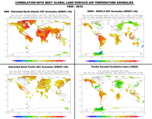
Figure 4
Full-sized version of Figure 4 is here.
WOULD USING DETRENDED NORTH PACIFIC SEA SURFACE TEMPERATURE DATA INSTEAD OF THE PDO DATA HAVE CHANGED THE RESULTS OF MULLER ET AL?
Nope. The AMO still has the strongest correlation with land surface air temperatures, because they both respond similarly to ENSO, ENSO residuals and volcanic aerosols.
But Muller et al could have saved themselves some time, since the PDO data does not in any way represent the sea surface temperatures of the North Pacific and there was, therefore, no reason to compare it to the AMO data.
ENSO RESIDUALS?
I mentioned ENSO residuals a couple of times in this discussion. Those residuals are basically the aftereffects of strong El Niño events, and those aftereffects are caused by the warm water that’s left over from those strong El Niños. My illustrated essay “The Manmade Global Warming Challenge” [42MB] provides an overview of the causes and impacts of those leftover warm waters. It includes links to animations of data, which confirm the existence and source of the ENSO residuals.
And, of course, if you’re very interested in learning more about the processes of El Niño and La Niña events, there’s my book Who Turned on the Heat? The free preview is available here. Who Turned on the Heat? is available in pdf form here for US$8.00.
FURTHER INFORMATION ABOUT THE AMO
A link to the NOAA FAQ webpage about the AMO is here. I provided a detailed introduction to the Atlantic Multidecadal Oscillation in my post here.
The short description: the Atlantic Multidecadal Oscillation is a mode of natural variability through which the sea surface temperatures of the North Atlantic can contribute additionally to or suppress the global warming of land surface air temperatures that are occurring in response to the warming of the rest of the global oceans. And as discussed in the “The Manmade Global Warming Challenge” [42MB], the ocean heat content data and satellite-era sea surface temperature data both indicate the oceans warmed naturally.
Refer also to the RealClimate glossary webpage about the Atlantic Multidecadal Oscillation here. There, they write:
A multidecadal (50-80 year timescale) pattern of North Atlantic ocean-atmosphere variability whose existence has been argued for based on statistical analyses of observational and proxy climate data, and coupled Atmosphere-Ocean General Circulation Model (“AOGCM”) simulations. This pattern is believed to describe some of the observed early 20th century (1920s-1930s) high-latitude Northern Hemisphere warming and some, but not all, of the high-latitude warming observed in the late 20th century. The term was introduced in a summary by Kerr (2000) of a study by Delworth and Mann (2000).
ADDITIONAL INFORMATION
An El Niño releases heat into the atmosphere, and surface temperatures around the globe in many places warm in response to the El Niño, and in other parts, they cool—with more locations warming than cooling, so the average global surface temperature warms in response to the El Niño. But the heat released into the atmosphere during the El Niño is not directly warming the surface in those remote locations. The surface temperatures outside of the tropical Pacific warm in response to changes in atmospheric circulation caused by the El Niño. The processes that cause those changes are discussed in minute detail in Trenberth et al (2002) Evolution of El Nino–Southern Oscillation and global atmospheric surface temperatures. Wang (2005) ENSO, Atlantic Climate Variability, And The Walker And Hadley Circulation discusses why the tropical North Atlantic warms in response to an El Niño.
CLOSING
Compared to a number of other sea surface temperature-based indices (and sea level pressure-based indices, which we didn’t discuss in this post), Muller et al (2013) found that global land surface temperatures correlate best with the Atlantic Multidecadal Oscillation. We illustrated and discussed the reason for this—the AMO data and land surface air temperatures respond similarly to ENSO, ENSO residuals, and volcanic aerosols.
We also discussed and illustrated why Muller et al (2013) should have used detrended North Pacific sea surface temperatures instead the PDO data for a proper comparison to the AMO.
And we used correlation maps to show the differences between the PDO and the sea surface temperature anomalies of the North Pacific. We also used the correlation maps of the PDO and ENSO with global temperature anomalies to help explain what the PDO represents.
There’s a global multidecadal oscillation and it can be seen in all global and non-global temperature indices. AMO is just a regional (north Atlantic SST) manifestation.
http://www.woodfortrees.org/plot/esrl-amo/plot/esrl-amo/trend/plot/hadcrut4gl/detrend:0.76/plot/hadcrut4gl/trend/detrend:0.76
One can use any global, hemispheric, land or sea temperature index and find the same oscillation.
Oops, forgot to note that the multidecadal variations in the sea surface temperatures of the North Pacific (north of 20N) can be comparable in magnitude to those in the North Atlantic, but they run in and out of synch with one another:
http://bobtisdale.files.wordpress.com/2013/05/figure-24.png
That graph is from the recent post Multidecadal Variations and Sea Surface Temperature Reconstruction:
http://bobtisdale.wordpress.com/2013/05/14/multidecadal-variations-and-sea-surface-temperature-reconstructions/
Nice critique. I am amazed though that Mullers co-authors have not been reading your posts here on WUWT and thus did not see to use the detrended North Pacific sea surface tempertatures.(instead of ENSO)
Ed_B says: “…and thus did not see to use the detrended North Pacific sea surface tempertatures.(instead of ENSO)”
I assume that’s a typo and that ENSO should be PDO.
Regards
Thank you Bob for another good piece of analysis.
Reality can be a damn problem.
“We’ll discuss why Muller should have included detrended North Pacific sea surface temperatures instead of the PDO in their comparisons with the AMO data, and we’ll use correlation maps to help show what the PDO represents—and what it doesn’t represent.”
It’s like pushing water uphill Bob. You inform repeatedly. People ignore repeatedly.
This has gone on for years — that’s too long. My patience with those who can’t or won’t get it has expired. I’m permanently writing them off as dumber-than-a-post. Under the bus they go…
Paul Vaughan says: “Under the bus they go…”
Speed bumps!
“Before it is safe to attribute a global warming or a global cooling effect to any other factor (CO2 in particular) it is necessary to disentangle the simultaneous overlapping positive and negative effects of solar variation, PDO/ENSO and the other oceanic cycles. Sometimes they work in unison, sometimes they work against each other and until a formula has been developed to work in a majority of situations all our guesses about climate change must come to nought.
So, to be able to monitor and predict changes in global temperature we need more than information about the past, current and expected future level of solar activity.
We also need to identify all the separate oceanic cycles around the globe and ascertain both the current state of their respective warming or cooling modes and, moreover, the intensity of each, both at the time of measurement and in the future.”
from here:
http://climaterealists.com/index.php?id=1302&linkbox=true&position=10
“The Real Link Between Solar Energy, Ocean Cycles and Global Temperature”
Wednesday, May 21st 2008, 8:20 AM EDT
The AMO is indeed a very important natural climate cycle driver.
Have a look at the monthly Raw AMO index versus Hadcrut4 back to 1856 (The Raw Index is not detrended and is not smoothed – I sometimes use this metric just to show how similar monthly temperatures are to the AMO).
http://s18.postimg.org/9uar3ow0p/Hadcrut4_vs_Raw_AMO.png
Now on a scattergram, not 100% close but the R^2 is 0.48 which on its own explains more of the temperature variability on a monthly basis than any other index).
http://s9.postimg.org/yi12i63z3/Hadcrut4_vs_Raw_AMO_Scatter.png
AMO data here.
http://www.esrl.noaa.gov/psd/data/timeseries/AMO/
This paper does serve a purpose later when the AMO is in obvious decadal decline. It helps blunt the cooling temperature deniers the random excuse such as declining or shifting Gulf Stream and other nonsense.
That’s the problem of an arbitrary index. It is chosen, and sometimes defined, by the person who wants to use it.
If a securities broker thinks the Dow Jones index isn’t saying what the broker wants to tell the clients, then he might choose the all-share index instead.
I’m really uncomfortable with the statement in the Muller paper: “<iThe long-term variability was suppressed by removing the least-squares fit 5th order polynomial from each curve.”.
That appears to me to be very arbitrary and very risky. Since a 5th order polynomial has no real-world meaning, there is no way of knowing whether it really does represent “long-term variability”. The act of removing it may be removing meaningful data, and could even actually be adding in meaningless data. What’s left after its removal does not necessarily have any real-world meaning since its value is the difference between “some real world stuff” and “some non real world stuff”.
In particular, the period studied was 1950-2010, which is only 60 years. It seems inevitable that some of the ‘5th order polynomial’ would necessarily represent much of whatever effect the AMO has – the very effect that is supposed to be visible after the 5th order polynomial has been removed. I don’t see how the Muller paper can be taken seriously.
Very interesting post! I was surprised to see that land temperatures in most of Europe correlate better with detrended North Pacific SSTs than with the AMO.
Comparing what Muller (et al) does with what science actually is is comparing apples with oranges.
Comparing what Muller (et al) does with funding … not so much.
Yes, they read WUWT. Anyone in their right mind would. Oh, yeah, sorry.
Black Diamond or Black Swan?
Take a moment of your time. If you can see that the logical extension of the UAH data series in this presentation should next contain a Black Diamond (a falling node) and can place it somewhere on the graph with good arguments as to why and when, then welcome to the world of short term climate prediction!
http://s1291.photobucket.com/user/RichardLH/story/70051
This is effectively just a presentation of the low frequency (1 to 15 years) natural cycles visible in the present in the satellite data (i.e. from 1979). That is, measured cycles, not proposed ones!
Nyquist limits the presentation to cycles less than 15 years in the output for now.
A black swan moment?
Here’s my view (again). The PDO is actually an indicator of the structure of global atmospheric pressure zones (GAPZ) – (think Bermuda high, or Aleutian Low). The average position of these GAPZs affect the jet streams. For example, a strong Bermuda High in 2012 led to a more northerly jet stream in the US which led to less precipitation and warmer temperatures.
At this geological blink of time the GAPZs have been cycling through a ~60 cycle. The PDO appears to be a good proxy for the GAPZ’s positions. When the PDO is positive as it was from 1976-2005 then several things occur:
– El Niño are more prevalent (which releases more heat into the atmosphere)
– The AMO index starts to increase. (which leads to more Arctic sea ice loss)
– More zonal jet streams (Which reduces global cloudiness/albedo slightly)
The opposite happens when the PDO becomes negative as is the case right now.
This can have interesting effects. For example, with a positive PDO the jet stream position over the N. Atlantic is driven higher (more northerly) allowing more sunshine over the water and the AMO to increase. However, this also causes the jet stream to dive down over Europe leading to cooler temperatures even while the North Atlantic is warmer.
Keep in mind that all of this refers to “average” positions.
This explains almost everything we’ve seen temperature-wise over the last 100 years. Of course, it doesn’t explain what drives the changes. There are several possibilities both terrestrial and non-terrestrial.
Richard M says:
June 18, 2013 at 7:48 am
Much as I’ve been suggesting since 2008.
Next step, consider what causes longer term variations beyond the 60 year cycle.
I suggest top down solar effects altering global albedo to skew ENSO towards El Nino or La Nina via cloudiness changes.
The latitudinal positions of the climate zones and jet streams serve as a proxy for changes in the energy budget such that zonal / poleward is a sign of warming and equatorward / meridional is a sign of cooling and in each case the circulation change is a negative system response to whatever the net forcing effect of all relevant mechanisms is at any given moment.
So, if the system tries to warm then the poleward zonal pattern lets energy flow through the system faster (less clouds) and if the system tries to cool then the equatorward meridional pattern causes energy to flow through the system more slowly (more clouds).
Richard M says:
June 18, 2013 at 7:48 am
“Keep in mind that all of this refers to “average” positions.
This explains almost everything we’ve seen temperature-wise over the last 100 years. Of course, it doesn’t explain what drives the changes. There are several possibilities both terrestrial and non-terrestrial.”
I would propose that natural cycles or 37 months, 4 years, 7 years (3+4) and 12 years (3*4) are of more than passing interest.
“We identify one strong narrow spectral peak in the AMO at period 9.1 ± 0.4 years and p-value 1.7% ”
Hey, that sounds a lot like Scafetta’s 9.01 +/-0.1 , which he identified as be lunar in origin. 😉
My article on lunar-solar influence:
http://climategrog.wordpress.com/2013/03/01/61/
identified this as a significant frequency in many basins. It also showed how Hadley manage to remove it from the SST record.
http://climategrog.files.wordpress.com/2013/03/icoad_v_hadsst3_ddt_n_pac_chirp.png
Maybe that is why it took a study of land temps to find this.
What a polite but total take down of the essay by Muller and friends. There are two major highlights:
“Many papers and blog posts attempt to remove the impacts of natural variables from the global surface temperature record. When they add AMO data to the ENSO, volcanic aerosol and solar data in their multiple regression analyses, do they recognize and account for the fact that the AMO data and global land surface air temperature data have similar responses to ENSO and volcanic aerosols?”
Let me restate this. Many people use purely statistical techniques to accomplish what they call “removing the impacts of natural variables” only to reveal that they are utterly clueless about the natural processes from which their data was taken. These people have the annoying habit of excluding from their work any and all hypotheses about the natural processes. (Even my version comes across as polite – must be the influence of Tisdale.)
The second point is that not only are Muller and friends uninterested in underlying physical processes but are inexplicably careless with the data obtained from them. Mr. Tisdale writes:
“A good portion of Muller et al (2013) deals with comparisons of global surface temperatures with the Atlantic Multidecadal Oscillation index (AMO) and with the Pacific Decadal Oscillation index (PDO), to emphasize their findings.
Muller et al (2013) failed to recognize that the AMO index data is detrended sea surface temperature anomalies of the North Atlantic, while the PDO index is NOT detrended sea surface temperature anomalies of the North Pacific. The PDO is an abstract form (a Picasso version, if you will) of the sea surface temperature anomalies of the North Pacific. So Muller et al (2013) were comparing apples to oranges.”
At this point, politeness is really difficult though Mr. Tisdale managed to be polite. After recovering from a powerful “face palm,” I am pretty much speechless. How could Muller and friends have overlooked this? How could journal reviewers have overlooked this? (Pardon my lack of politeness, but this matter raises a serious question of trust.)
Greg Goodman says:
June 18, 2013 at 8:54 am
“Maybe that is why it took a study of land temps to find this.”
This is a summary of observed short term (< 15 years) cycles in the satellite data.
http://s1291.photobucket.com/user/RichardLH/story/70051
Thanks, Bob.
You have reported on reality, but many deny the real, too complex world and then device models that reflect only their own preconceptions.
Paul Vaughan says, June 18, 2013 at 5:00 am:
“You inform repeatedly. People ignore repeatedly. This has gone on for years — that’s too long. My patience with those who can’t or won’t get it has expired.”
I couldn’t agree more. People still act as though Tisdale’s strictly data-based explanation of global warming since the 70s doesn’t exist and has never been put forward, on this blog or his own, or elsewhere. You can see posts back-to-back with Tisdale expositions of how it all went down acting all confused about the recent ‘pause in warming’ or how there really has been warming over the last 35 years so there should be a certain CO2 component in there somewhere (read: climate sensitivity studies). People are still lamenting the level of scientific knowledge about what really rules the climate, as if there are somehow huge gaps in our understanding, some missing and as of yet unknown mechanisms pulling the strings. And yet they’re bound to have read or at least heard of this guy called Bob Tisdale at some point during the last four years showing us all that ENSO is the natural process doing the pulling – the Great Puppet Master – not just on an interannual or decadal scale, but on a multidecadal one. There is hardly a gap in our understanding of what caused the global warming since the 70s, which clearly and obviously is contained in its entirety within three abrupt shifts. Not for those of us who care to have a look at what the real-world data are actually telling us. Bob Tisdale has, once and for all, rid us of the need for any CO2 ‘God of the Gaps’ … And he’s still summarily ignored or dismissed. I wonder what kind of psychological or sociological phenomenon that lies behind.
Muller et al “suppressed” the “long-term variability” by subtracting the values of a 5th order polynomial curve from the data.
Curious wording on their part. Usually that is called “detrending”.
Espen says, June 18, 2013 at 6:49 am:
“I was surprised to see that land temperatures in most of Europe correlate better with detrended North Pacific SSTs than with the AMO.”
I think you will find that European temperatures correlate most tightly with the AO/NAO mode.
Muller et al (2013) failed to recognize that the AMO index data is detrended sea surface temperature anomalies of the North Atlantic, while the PDO index is NOT detrended sea surface temperature anomalies of the North Pacific. The PDO is an abstract form (a Picasso version, if you will) of the sea surface temperature anomalies of the North Pacific.
I take it you were not satisfied with the detrending carried out by Muller et al. What can you possibly mean by “a Picasso version”?
And based on our earlier discussion, the reason the AMO has a positive or neutral correlation with global surface temperatures almost everywhere is, the AMO and global surface temperatures respond similarly to ENSO, ENSO residuals and volcanic aerosols. Simple.
I noticed that here and elsewhere you accepted a main result of Muller’s analysis while exploring interpretations that they have slighted or ignored.
It’s a shame you won’t submit your work for publication.
Matthew R Marler says:
June 18, 2013 at 9:31 am
“It’s a shame you won’t submit your work for publication.”
Why?
“Greg Goodman says:
June 18, 2013 at 8:50 am
“We identify one strong narrow spectral peak in the AMO at period 9.1 ± 0.4 years and p-value 1.7% ”
Hey, that sounds a lot like Scafetta’s 9.01 +/-0.1 , which he identified as be lunar in origin. ;)”
#########
that would kinda explain why we cite him and discuss it. doh. the benefits of reading a paper before commenting are sometimes large.
“Scafetta [2010] reported a forest of 11 spectral
peaks based on a multitaper analysis; to each of these peaks,
he calculated 99% confidence intervals. He reported seven
peaks with periods in the range from 5.99 to 14.8 years.
One of these is at our period of 9.1 years; he suggests that this
cycle could be induced by lunar tidal variations. However,
we find that when we use our Monte-Carlo methods to estimate background, none of his claimed peaks are statistically
significant except for the 9.1 year peak; we do not find them
in the AMO, PDO, or ENSO.”
Matthew R Marler says: “I take it you were not satisfied with the detrending carried out by Muller et al.”
Nope, my complaint was that they used the PDO index data instead of detrended sea surface temperature anomalies of the North Pacific.
Matthew R Marler says: “What can you possibly mean by “a Picasso version”?”
Picasso, if memory serves, was a one of the first cubists. Cubism is a form of abstract art. The PDO is an abstract portrayal of the sea surface temperatures of the North Pacific.
Bhb Tisdale says:
June 18, 2013 at 10:39 am
When creating a portrait, Picasso would on occasion show the subject in multiple perspectives at the same time. To the untrained eye, some of his subjects seemed to have three noses trying to fit in the same spot. Picasso’s work gave rise to an industry of critics who explained how these portraits are to be viewed. Time revealed that there is no rational explanation of how to view these portraits. Mr. Tisdale chose a very good analogy.
This paper is interesting for several reasons.
The first reason is that it was received by JGR on the 22nd of April 2013; it was revised on the 28th of April 2013; and it was accepted on the 30th of April 2013.
I would love to receive such speedy review for my own papers.
The second reason why this paper is very interesting is because it contains one important result, that is that the AMO and the PDO are characterized by a significant quasi 9.1 year oscillation. The only major problem with this important “discovery” is that this about 9.1 year oscillation in the AMO and PDO indexes was actually discovered and extensively discussed in one of my papers, see for example figure 9 in:
Manzi V., R. Gennari, S, Lugli, M. Roveri, N. Scafetta and C. Schreiber, 2012. High-frequency cyclicity in the Mediterranean Messinian evaporites: evidence for solar-lunar climate forcing. Journal of Sedimentary Research 82, 991-1005. DOI: 10.2110/jsr.2012.81.
http://people.duke.edu/~ns2002/pdf/991.full.pdf
which, of course, was not referenced. My analysis is actually better.
Fortunately, they referenced one of my past papers
Scafetta N., 2010. Empirical evidence for a celestial origin of the climate oscillations and its implications. Journal of Atmospheric and Solar-Terrestrial Physics 72, 951-970.
DOI: 10.1016/j.jastp.2010.04.015.
http://people.duke.edu/~ns2002/pdf/ATP3162.pdf
where the 9.1 year oscillation is also discovered in the global temperature records around he earth and it was demonstrated that it is very likely a soli-lunar long-range tidal cycle which should be particularly strong in the ocean related record such as the PDO and AMO.
A better explanation of this soli-lunar tidal cycle is discussed in page 35-36 of the supporting material of
Scafetta N., 2012. Testing an astronomically based decadal-scale empirical harmonic climate model versus the IPCC (2007) general circulation climate models. Journal of Atmospheric and Solar-Terrestrial Physics 80, 124-137.
DOI: 10.1016/j.jastp.2011.12.005.
http://people.duke.edu/~ns2002/pdf/ATP3533.pdf
which they do not reference either.
Then there are other minor issues such as their proposed ““prewhitening” process made with a 5-order polynomial that is a very rude and very dangerous high-pass filter that would partially deform also the high component of the spectrum (fortunately only a little bit). And other details such as their claim that I found a “forest” of 11 spectral based on a “multitaper analysis”, which is false because I am mostly using the Maximum Entropy Method which is far more accurate, and other small details such as the AMO and PDO present an oscillation closer to 60-year than a 70-80 year one of the model.
However, given the fast review of the paper, I do not expect that the reviewer had much time to give a look around or study statistics.
But the paper is interesting, nevertheless. A better review would have improved it.
1. The correlation of .65 +/- .04 is a very moderate correlation, to show strong correlation one must show >.85 — Even with strong correlation the following quote from the paper stands, “Correlation does not imply causation.”
2. The author’s suggestion of only using north pacific SST during the PDO phase is intriguing and will show stronger correlation though the correlation will be negative. The reason this is true is because the south hemisphere’s effect (cooling) is stronger. . .this is based on the following quote from the article,
“An El Niño releases heat into the atmosphere, and surface temperatures around the globe in many places warm in response to the El Niño, and in other parts, they cool—with more locations warming than cooling, so the average global surface temperature warms in response to the El Niño. But the heat released into the atmosphere during the El Niño is not directly warming the surface in those remote locations. ”
conversely, a La Nino cools the atmosphere by allowing more atmospheric heat energy to enter the oceans. (please note that the atmospheric energy is also entering the oceans during El Nino, just not as much as neutral and La Nina phases.
3. The Berkeley Earth Temp Project summary of findings. says,
“The good match between then new temperature record and historical carbon dioxide records suggests that the most straightforward explanation for this warming is human greenhouse gas emissions.”
This indicates that the relatively low correlation of El Nino and AMO to Land Surface temperatures does not IN ANY WAY detract from the reality of anthropogenic climate change as currently understood and caused by the increase of greenhouse gasses. (the low correlation of El Nino and AMO only displays a shift in the energy balance between ocean and atmosphere and does not in any way show more or less warming).
4. This is only another “wake up call” that indicates we need to be more concerned with land surface temperatures and not sea surface temperatures and definitely not lower-correlation satellite tropospheric temperatures that do not show northern hemisphere land temperature amplification (where most of humanity lives and grows food).
I am a big fan of Dr. Muller. . .by the way.
I’m a little confused here. If they removed this signal from the temperatures:
http://bobtisdale.files.wordpress.com/2013/06/amo-with-5th-order-polynomial.png
…didn’t they remove precisely what they might be looking for?
New paper on North Atlantic SSTs published today in the Holocene going back to 1000 AD. Looks a little different than other AMO reconstructions we have seen but 10 different reliable-type proxies were used in this study.
http://hol.sagepub.com/content/23/7/921.abstract?rss=1&utm_source=feedly
Reconstruction (with a little help from me on conversion to temp-anomaly type numbers).
http://s8.postimg.org/5a2g4xnc5/North_Atlantic_SST_Proxies.png
Data here.
ftp://ftp.ncdc.noaa.gov/pub/data/paleo/paleocean/by_contributor/cunningham2013/cunningham2013-data-series.txt
Nicola,
on section 6 page 36 you show the 9.1 year harmonic cycle. It shows a temperature variance of .09C peak-to-trough as caused by the sol-lunar cycle that you hypothesize causes this temperature variability.
questions:
-you have no error bars on your graphic
1. what are the uncertainties of these values?
In your paper you state,
“Finally, there may be an additional natural warming due to
multisecular and millennial cycles as explained in Introduction. In
fact, the solar activity increased during the last four centuries
(Scafetta, 2009), and the observed global surface warming during
the 20th century is very likely also part of a natural and persistent
recovery from the Little Ice Age of AD 1300–1900”
—
and yet, you offer no hypothesized mechanism for this recovery, however, you penalize the “observed anthropogenic warming” based on this unsupported claim, you go on to say,
“Thus, the above estimated 1:30 1C=century anthropogenic warming
trending is likely an upper limit estimate. As a lower limit we
can reasonably assume the 0:6670:16 1C=century, as estimated in
Loehle and Scafetta (2011), which would be compatible with the
claim that only 0.2 1C warming (instead of 0.7 1C) of the observed
0.5 1C warming since 1970 could be anthropogenically induced”
and then use this in your models.
2. Don’t you think it is intellectually dishonest to assume an effect, without determining causality and in opposition to the preponderance of supportive evidence, and then use that assumption as an input for the production of a modeled result? Isn’t this, in effect, the epitome of “quasi-science”?
Unless you have a provable theory of causality for the “Jupiter effect” that you use as an excuse for a “recovery” from the little ice age, your results are incredibly suspect.
But fortunately this paper neither mentions carbon dioxide, nor makes such a foolish statement.
4. This is only another “wake up call” that indicates we need to be more concerned with land surface temperatures and not sea surface temperatures and definitely not lower-correlation satellite tropospheric temperatures that do not show northern hemisphere land temperature amplification (where most of humanity lives and grows food).
When ocean cycles are removed, land surface and sea surface temperature should be strongly correlated if CO2 is the cause (assuming constant humidity). They are not. Which tells us several things, including that land surface warming isn’t cause by a uniform global phenomena, and hence CO2 can not be the cause of land surface warming.
Otherwise, show me a correlation in the raw data and I’ll take notice.
jai mitchell says: June 18, 2013 at 11:51 am
I think that you are quite confused and should study the papers better.
1) the error on the 9.1 year is about 0.2 year and it is reported in Table 2 of
Scafetta N., 2010. Empirical evidence for a celestial origin of the climate oscillations and its implications. Journal of Atmospheric and Solar-Terrestrial Physics 72, 951-970.
DOI: 10.1016/j.jastp.2010.04.015. http://people.duke.edu/~ns2002/pdf/ATP3162.pdf
2) the other calculations you are talking about are not arbitrary, but based on the existence of a 60-year oscillation that very likely contributed 0.3 C warming between 1970 and 2000, which imply that AGW has been overestimated by 50-60% at least.
3) ” Don’t you think it is intellectually dishonest to assume an effect, without determining causality and in opposition to the preponderance of supportive evidence”
Not really, the models fail to properly interpret the 1970-2000 period for the same reason they fail to interpret the 1850-1880 warming, the 1910-1940 warming and the 1880-1910 and 1940-1970 cooling, and also the standstill since 2000. They also fail to get many other things, which would be to long here to say. So, your “preponderance of supportive evidence” does not exist. It is political propaganda, indeed.
For example if you do not want to look at my papers with any care, look at this figure prepared by Spencer that shows the epic failure of 73 Climate Models vs. Measurements, Running 5-Year Means:
http://www.drroyspencer.com/2013/06/still-epic-fail-73-climate-models-vs-measurements-running-5-year-means/
and try to respond to my question: which model reproduce the temperature?
Tell me one name and model run number
So it is legitimate to assume the existence of “causes” that the modelers do not know yet, and there are papers showing this pattern in the solar records. What I do is to investigate the dynamical implication of this “causes”. This is a valid argument in physics. And my models are tested in their forecasting capability and are good indeed. See here
http://people.duke.edu/~ns2002/#astronomical_model-1
What is really dishonest in science is to assume that everything should be already known and “settled” even when the proposed models do not reproduce the data and accuse those that investigate the missing physics of “dishonesty”.
“Nicola Scafetta says:
June 18, 2013 at 11:06 am
This paper is interesting for several reasons.
The first reason is that it was received by JGR on the 22nd of April 2013; it was revised on the 28th of April 2013; and it was accepted on the 30th of April 2013.”
##############################
The paper was submitted to JGR in 2011, reviewed and accepted at that time. JGR added the stipulation that final publication would be contingent on the publication of Rohde. once rohde 2012 was published the process went quickly as the paper had already been reviewed and accepted.
“However, given the fast review of the paper, I do not expect that the reviewer had much time to give a look around or study statistics.
But the paper is interesting, nevertheless. A better review would have improved it.”
#############################
From 2011 till today the paper has been available on our website. I searched my files for your comments. I find no emails from you.
So basically we made the paper freely available.
the data is freely available
the code is freely available.
The only thing stopping people from sending a mail or asking a question is….? I dunno.
It’s pretty simple. We post up our work in progress. Anybody who wants to ask me a question about it can do so. steve@berkeleyearth.org
If you are in the area and would like to come to my wen meeting to discuss issues with the head scientist, just let me know. Door’s open.
Nicola,
thank you for your reply.
I was not asking for the periodicity error that is in table 2. I was asking for the AMPLITUDE error which is the temperature error (which I mentioned as being .09C from peak to trough). Please provide (what you believe is) the temperature error sensitivity for the oscillation chart found on page 36 of the supplementary data.
————-
with regard to “quasi-science” you have answered the question phenomenally. . .you believe that it is ok to ascribe a causation based simply on periodicity and your understanding of the model. You even assume that this will work on a multi-centennial timescale with no corroborative evidence.
Bill illis
Your post at 11.51
Your middle graph headed S8 posting bears more than a passing resemblance to my cet reconstruction to 1538 and (very) interim generalised findings to 1210.
Can you tell me any more about it?
Tonyb
Phil Bradley,
When ocean cycles, solar cycles and volcanic eruptions are removed as “noise” from the data the temperature record absolutely pairs with the CO2 increase. This can be clearly found using multiple sources.
jai mitchell says:
June 18, 2013 at 1:25 pm
So, you too believe that the “forcings and feedbacks calculation” is complete and settled. Would you care to present it? What is the calculation for water vapor? How about cloud albedo?
jai mitchell say: June 18, 2013 at 1:20 pm
as I said, you may need to study my paper better. The amplitude uncertainties are reported for example at page 131 and there is a 20% error in the amplitudes of
Scafetta N., 2012. Testing an astronomically based decadal-scale empirical harmonic climate model versus the IPCC (2007) general circulation climate models. Journal of Atmospheric and Solar-Terrestrial Physics 80, 124-137. DOI: 10.1016/j.jastp.2011.12.005.
http://people.duke.edu/~ns2002/pdf/ATP3162.pdf
“You even assume that this will work on a multi-centennial timescale with no corroborative evidence.”
Not really, you need to study better the extended model here:
Scafetta N., 2012. Multi-scale harmonic model for solar and climate cyclical variation throughout the Holocene based on Jupiter-Saturn tidal frequencies plus the 11-year solar dynamo cycle. Journal of Atmospheric and Solar-Terrestrial Physics 80, 296-311.
DOI: 10.1016/j.jastp.2012.02.016
http://people.duke.edu/~ns2002/pdf/ATP3581.pdf
Steven Mosher says: June 18, 2013 at 12:46 pm
Ok Steven, I see what you want to say. However the paper appears “submitted” and received by JGR on the 22nd of April 2013; it was even revised on the 28th of April 2013; and it was accepted on the 30th of April 2013. As it is written on the web-site. Even if the paper was available in some draft form in 2011 the fact is that if the paper was resubmitted in 2013 it had to be updated with the available literature that extended since then. And written better given the large time they had to improve it and the numerous “email” comments that you say they received to improve it.
For example, when they say that they could find only the 9.1 year oscillation, somebody should have let them notice that by filtering the records with a 5-polynomial fit they were killing for example both the 20 and 60 year oscillation that are the other two major oscillations that I found and that I used the MEM and not the “multitaper analysis” etc.
In any case, please note that the fact that the ocean temperature records (AMO is a subset of the SST) presents a major 9.1 year oscillation has been clearly demonstrated by me in 2010.
Scafetta N., 2010. Empirical evidence for a celestial origin of the climate oscillations and its implications. Journal of Atmospheric and Solar-Terrestrial Physics 72, 951-970.
DOI: 10.1016/j.jastp.2010.04.015.
http://people.duke.edu/~ns2002/pdf/ATP3162.pdf
see figure 6B.
I hope that you acknowledge that 2010 is earlier than 2011. Because they reference my 2010 paper they should have noted that I was talking about the ocean records too and referenced my paper more properly instead of just writing a naïve and imprecise comment about my paper.
On another topic, about Rhode 2012 paper you may be interested in
Scafetta N., 2013. Discussion on common errors in analyzing sea level accelerations, solar trends and global warming. Pattern Recognition in Physics, 1, 37–57. DOI: 10.5194/prp-1-37-2013.
http://people.duke.edu/~ns2002/pdf/prp-1-37-2013.pdf
there is some comment on Rhode 2012 too and their way to use regression to interpret the temperature since 1700. See section 3.
If you’re designated troll today, jai mitchell, you need to find a new job. All you’ve managed to do on this thread is highlight your confusion about the subject matter.
jai mitchell says: “The author’s suggestion of only using north pacific SST during the PDO phase is intriguing…”
Did Muller et al suggest that? I didn’t, and I’m the author of this blog post. You seem confused.
jai mitchell says: “…conversely, a La Nino cools the atmosphere by allowing more atmospheric heat energy to enter the oceans. (please note that the atmospheric energy is also entering the oceans during El Nino, just not as much as neutral and La Nina phases.”
Wrong. You’re very confused about this.
The tropical Pacific releases heat primarily through evaporation. During a La Niña, the atmosphere cools because the sea surface temperatures are cooler and there is less evaporation. During an El Niño, the sea surface temperatures are warmer and there is more evaporation, and the result is a warmer atmosphere. Overall, during an El Niño, the tropical Pacific discharges heat. During a La Niña, the heat is recharged through an increase in sunlight. Basic ENSO.
jai mitchell says: “4. This is only another “wake up call” that indicates we need to be more concerned with land surface temperatures and not sea surface temperatures…”
You’re confused about this as well.
First, the warming of land surface air temperatures is primarily as response to the warming of the oceans. See Compo and Sardeshmukh (2009) “Oceanic Influences on Recent Continental Warming.”
http://www.esrl.noaa.gov/psd/people/gilbert.p.compo/CompoSardeshmukh2007a.pdf
The abstract begins:
“Evidence is presented that the recent worldwide land warming has occurred largely in response to a worldwide warming of the oceans rather than as a direct response to increasing greenhouse gases (GHGs) over land.”
Second, if you were to research it further, you’d discover the warming of sea surface temperatures were responsible for about 85% of the warming of land surface temperatures over the past 3 decades.
Third, as we all know, the ocean heat content data and satellite-era sea surface temperature data both indicate the oceans warmed naturally:
http://bobtisdale.files.wordpress.com/2013/01/the-manmade-global-warming-challenge.pdf
jai mitchell continued: “…and definitely not lower-correlation satellite tropospheric temperatures that do not show northern hemisphere land temperature amplification (where most of humanity lives and grows food).”
I’m not sure what planet you live on, jai mitchell, but RSS and UAH TLT anomalies both show polar amplification:
http://oi40.tinypic.com/dwv236.jpg
Nicola
I see the error calculation you have for your sinusoidal coefficients. They are .03 +/- .01 for the first term and .05 +/- .01 for the second.
so is the error range 20% or 33%
and how did you determine these values?
Oh I see! Thanks for the multi-scale harmonic model paper
where you say,
It is not possible to accurately reconstruct the amplitudes of the
solar dynamical patterns. Such exercise would be impossible also
because the multi-decadal, multi-secular and millennial amplitudes
of the total solar luminosity and solar magnetic activity are
extremely uncertain (p297)
So the amplitude of this sinusoidal wave function is basically just a guess, correct?
———-
you have done significant work on these papers, I don’t mean to fault them in toto because they do show a very interesting dynamic. That being said, the methodology of
A. determining a periodicity in the record
B. Knowing full well that other planets have as much or greater influence on the sun (i.e earth exerts 95.3% of the force of Saturn on the sun and Venus exerts more force than Saturn) You still only use the tidal patterns of Jupiter and Saturn.
C. This is all interesting but if you want to perform a best fit model you will have to, I repeat MUST, produce a tidal force model using AT LEAST the first 5 planets combined. You simply cannot produce a reasonably effective solar model without including the orbits of mercury-mars in your calculations.
—————
If you do have a hypothesized effect of planetary tidal forces on the internal circulation models of the sun then you cannot exclude the other planets from the model. It just won’t work and makes the entire exercise seem more like trickery.
I would like to see this done, you have put a lot of work into this!
Steven Mosher says: June 18, 2013 at 12:46 pm
Moreover, Steven, consider that my Figure 6B in my 2010 paper demonstrates a full spectral coherence among alternative regions of the Earth (North and South, Ocean and Land), which demonstrate a full synchronicity of the climate system. I talk extensively about this synchronicity in the paper.
Essentially only figure 6B of my paper by alone says much more than Muller’s paper claiming to demonstrate that there is a link between AMO and temperature.
And my paper says even much more by providing a physical interpretation of the spectral findings that they could not understand.
Muller et al. could only reference my 2010 paper talking about “a forest” about things that they do not understand.
jai mitchell says June 18, 2013 at 3:28 pm
1)
“So the amplitude of this sinusoidal wave function is basically just a guess, correct?”
Not really, the amplitudes must be calculated from regression from the data. You apparently do not understand that an identical methodology is used to predict the tides. People measure the amplitudes from regression from the data. See here
http://en.wikipedia.org/wiki/Theory_of_tides#Tidal_analysis_and_prediction
The astronomical theory gives the frequencies, not the amplitudes.
2) “I repeat MUST, produce a tidal force model using AT LEAST the first 5 planets combined. You simply cannot produce a reasonably effective solar model without including the orbits of mercury-mars in your calculations.”
Again you are not reading my papers. What you say using all planets is done here
Scafetta N., 2012. Does the Sun work as a nuclear fusion amplifier of planetary tidal forcing? A proposal for a physical mechanism based on the mass-luminosity relation. Journal of Atmospheric and Solar-Terrestrial Physics 81-82, 27-40.
DOI: 10.1016/j.jastp.2012.04.002
http://people.duke.edu/~ns2002/pdf/ATP3610.pdf
But it is irrelevant because the effects of the Venus, Mercury and Earth is to produce very fast tidal oscillations. These are not of the order of 10-12 years and above, but of a few months to 1 year.
Note that even if Venus, Mercury produce large theoretical tides (smaller than jupiter), because they are fast they are also smoothed out by internal solar dynamics inertia. So, on the decadal and above scales it is Jupiter and Saturn and possible the other planets that matter.
But the issue is not yet fully developed.
I hope that you understand that doing scientific research means to proceed step by step and this does not mean to be “dishonest” as you accused
Bob Tisdale
As usual, you don’t even bother to read my posts before responding to it. I said the author of THIS article (you), not Muller.
YOU said,
If Muller et al (2013) had compared the AMO data (upper left-hand map) with a comparable dataset from the North Pacific (north of 20N) they would have used detrended North Pacific sea surface temperature anomalies (lower left-hand map), because the AMO index is detrended sea surface temperature data from the North Atlantic. Instead they used the PDO, which does not represent the sea surface temperatures of the North Pacific.
and I took that to mean,
“The author’s suggestion of only using north pacific SST during the PDO phase is intriguing. . .”
would you care to restate more clearly what you mean by a
“comparable dataset from the north pacific” (instead of including the south pacific values as was used in the PDO analysis)
————————
Bob, if you believe, in any universe, that the tropical ocean, as a whole body of water, acts as a net source of heat on planet earth, AT ANY TIME DAY OR NIGHT, EL NINO OR LA NINA.
then you need to go back to grade school and take a physics class.
http://oceanworld.tamu.edu/resources/oceanography-book/oceansandclimate.htm
————————–
The simple fact is that a slightly higher sea surface temperature in a single region (El Nino) cannot compensate for the average overall temperature of the entire ocean. Yes, there will be an increase in evaporation (where does this latent heat of evaporation energy come from? do you know?) But the overall net energy balance of the ocean in the tropics is highly negative (as opposed to the higher latitudes where it is positive. . .)
That is why we have the ocean currents.
—————————-
That oceanic influences on continental warming paper was cute. It doesn’t prove in any way, shape, or form, that the surface land heating was ONLY caused by ocean surface warming. The warming of Siberia and The Canadian Archipelago is currently being caused by shifts in the jet stream, same with the snow cover anomalies. They have NOTHING to do with sea surface temperatures.
what you are showing me is a misattribution to the author followed up with a pathetic excuse that is the equivalent of the BIG LIE (sea surface temperatures are natural). When the fact is that human produced greenhouse gasses are going to absolutely destroy our culture and society. And you will be finding that out very quickly now.
enjoy the additional 5-8C warming that we will begin to experience in the arctic in the next decade.
http://www.colorado.edu/geography/class_homepages/geog_4271_f10/readings/week_10_lawrence_et_al_2008.pdf
Keep watching this graphic:
http://home.comcast.net/~ewerme/wuwt/cryo_compare.jpg
when you figure out how real and existential this threat is, let me know, and if it isn’t too late, let me know what you plan to do about it.
enjoy the additional 5-8C warming that we will begin to experience in the arctic in the next decade.
============
jai, are you saying temps will increase 5-8C in the next decade….and we will experience that
-or-
are you saying temps will eventually get to 5-8C…and in the next decade we will experence the beginning of that increase
@ jai mitchell
have I got this right? – you think a bucket load of heat is currently stored in the oceans and is gonna cause lots of future warming? (5-8 degC ?) I think it only reasonable to ask for some evidence/links for this statement!
jai mitchell says:
“Enjoy the additional 5-8C warming that we will begin to experience in the arctic in the next decade.”
That is proof enough for me that mitchell has gone off the deep end.
The noob, wet-behind-the-ears jai mitchell also tells Bob Tisdale:
“…you need to go back to grade school and take a physics class.”
Either mitchell has never taken a physics class himself, or he is as deluded a climate alarmist as I have seen recently. It is to Anthony’s creeit that he allows scientific illiterates like mitchell to comment here. That way, readers can easily see who really needs to take a physics class.
Tonyb says:
June 18, 2013 at 1:24 pm
———————
I don’t know much more about it other than it is from a new paper published today that used 10 different proxies that cover most of the North Atlantic and most of the series go back to 1000 AD. The proxies are mostly δ18O from foraminifera which in my travels around the paleoclimate appear to be the most reliable temperature proxies. They are the best.
paper here.
http://hol.sagepub.com/content/23/7/921.abstract?rss=1&utm_source=feedly
All the different data series and further notes here.
ftp://ftp.ncdc.noaa.gov/pub/data/paleo/paleocean/by_contributor/cunningham2013/
A collation of all of them is here – last column NENA_Comp is a composite of all of them.
ftp://ftp.ncdc.noaa.gov/pub/data/paleo/paleocean/by_contributor/cunningham2013/cunningham2013-data-series.txt
Since we were talking about the AMO, I thought it relevant to bring up.
The net effect of all oscillations, named or not, must be considered simultaneously when determining average global temperature. This is done in the paper at http://climatechange90.blogspot.com/2013/05/natural-climate-change-has-been.html . This paper presents a simple equation that calculates average global temperatures since they have been accurately measured world wide (about 1895) with an accuracy of 90%, irrespective of whether the influence of CO2 is included or not. The only external forcing in the equation is a proxy which is the time-integral of sunspot numbers. A graph is included which shows the calculated trajectory overlaid on measurements.
‘The End of Global Warming’ at http://endofgw.blogspot.com/ expands recent (since 1996) temperature anomaly measurements by the five reporting agencies and includes a graph showing the growing separation between the rising CO2 and not-rising average global temperature.
jai mitchell says: “would you care to restate more clearly what you mean by a ‘comparable dataset from the north pacific’ (instead of including the south pacific values as was used in the PDO analysis)”
Fine, let me rephrase that paragraph for you, even though it was stated elsewhere numerous times in the post. AMO data is detrended sea surface temperature anomalies of the North Atlantic. The PDO is not detrended sea surface temperature anomalies of the North Pacific. Therefore, the PDO is not comparable. Detrended sea surface temperature anomalies of the North Pacific would have been comparable.
jai mitchell says: “Bob, if you believe, in any universe, that the tropical ocean, as a whole body of water, acts as a net source of heat on planet earth, AT ANY TIME DAY OR NIGHT, EL NINO OR LA NIÑA…then you need to go back to grade school and take a physics class.”
Everything I’ve presented in my blog posts and books over the past 4 years is supported not only by physics, it’s supported by data. It’s supported by ocean current data, trade wind strength and direction data, sea surface temperature data, ocean heat content data, downward shortwave radiation (sunlight) data, downward longwave (infrared) radiation data, cloud amount data, precipitation data, warm water volume data, depth-averaged temperature data, sea surface height data, etc.
jai mitchell says: “The simple fact is that a slightly higher sea surface temperature in a single region (El Nino) cannot compensate for the average overall temperature of the entire ocean.”
What you had written earlier pertained to El Niño and La Niña events, which take place in the tropical Pacific. But now you’ve magically shifted to global sea surface temperatures after your earlier comments were shown to be nonsense. In other words, you’re simply shifting your area of obvious confusion.
If you would take your blinders off and examine the sea surface temperature data and ocean heat content data as I’ve presented them in the following, you would note that there is nothing in either record to indicate any influence of human-induced global warming:
http://bobtisdale.files.wordpress.com/2013/01/the-manmade-global-warming-challenge.pdf
jai mitchell says: “That oceanic influences on continental warming paper was cute…”
Why would you say it was cute? Compo and Sardeshmukh performed an exhaustive analysis of your beloved climate models, and that’s what the climate models say. Once again, you’ve shown you can’t grasp what’s being presented to you.
jai mitchell says: “It doesn’t prove in any way, shape, or form, that the surface land heating was ONLY caused by ocean surface warming.”
And again, jai mitchell, you’ve highlighted for everyone reading this thread that you cannot comprehend what I’d written. I did not write that “surface land heating was ONLY caused by ocean surface warming.” Go ahead, go back and reread what I wrote in my last reply to you.
jai mitchell says: “The warming of Siberia and The Canadian Archipelago is currently being caused by shifts in the jet stream, same with the snow cover anomalies. They have NOTHING to do with sea surface temperatures.”
Do you realize you’ve just stated that natural variability, changes in jet stream location, can cause warming? That’s yet another indication that you’re a very confused person.
Are you aware that the oceans and atmosphere are coupled, jai mitchell? Do you understand what I mean by coupled?
Do you have any idea what causes shifts in jets streams, jai mitchell? Suppose I link a NOAA webpage that showed you that El Niño and La Niña events were one of the primary causes for shifts in the jet streams, which means that the locations of jet streams are, in fact, caused by changes in sea surface temperatures. Since you do not appear to have any technical background, I’ll link the NOAA webpage that’s easiest to understand:
http://www.srh.noaa.gov/jetstream/tropics/enso_impacts.htm
jai mitchell says: “When the fact is that human produced greenhouse gasses are going to absolutely destroy our culture and society. And you will be finding that out very quickly now.”
Your nonsensical alarmism doesn’t fly here, jai mitchell. You, like most of your ilk, show no grasp of the subject matter.
Adios, troll.
Oops, I missed your closing, jai mitchell.
jai mitchell says: “when you figure out how real and existential this threat is, let me know, and if it isn’t too late, let me know what you plan to do about it.”
What do I plan to do about it? I plan to continue to write blog posts and books to help re-educate the public about the natural causes of global warming. And I plan to continue to be entertained by nonsensical comments from brainwashed, clueless alarmist trolls just like you. I do find you very entertaining, jai mitchell.
Theo Goodwin (June 18, 2013 at 8:56 am) asked:
“How could Muller and friends have overlooked this? How could journal reviewers have overlooked this? (Pardon my lack of politeness, but this matter raises a serious question of trust.)”
I guess you might call it politics.
The other possibility is they’re dumber-than-a-post.
Bob,
you believe that the tropical ocean sometimes acts as a heat source, in contrast to the reality that the tropical oceans are the largest single heat sink on the planet, that the suns energy is primarily absorbed in the tropical seas and then transported via ocean currents to the northern latitudes. You have apparently written volumes about this but can still somehow defy the laws of thermodynamics and claim that the tropical ocean can act as a heat source.
The extreme Jetstream activity that has been occurring lately is not caused by natural variability. Your pathetic assertions that that they are show how desperate you have become trying to defend your insane ideology. There isn’t a single person in the northern hemisphere who doesn’t know that the weather is getting weirder and weirder. The simple fact that you cannot allow discussion about this shows how you are finally being proven as the dishonest fossil fuel industry shill that you are.
If you made even the most simple and honest inquiry to understand this you would have realized that the Arctic amplification has fundamentally changed the operations of the Jet Stream. That this was observed and documented in 2007 and predicted after the ice melt of 2012.
I can’t believe Judith Curry allowed herself to be named as an author of something so amateur.
For anyone who questions the 5-8C warming in the arctic.
it was related to the linked paper that describes the change that will occur there once the sea ice has melted. While there is significant arctic sea ice, the phase transformation that occurs (melting) is Isoclinic (stuck at 32’F) once the rest of the ice has melted, the energy that melted the ice in previous years will now lead to rapid temperature rises of sea surface and land surfaces. This is clearly shown in the following links.
————–
enjoy the additional 5-8C warming that we will begin to experience in the arctic in the next decade.
http://www.colorado.edu/geography/class_homepages/geog_4271_f10/readings/week_10_lawrence_et_al_2008.pdf
Keep watching this graphic:
http://home.comcast.net/~ewerme/wuwt/cryo_compare.jpg
when you figure out how real and existential this threat is, let me know, and if it isn’t too late, let me know what you plan to do about it.
not *isoclinic* , I meant isothermal. . .Latent heat of fusion. . .
jai mitchell,
It doesn’t matter what you meant. We know you’re only starting to get up to speed on the subject.
And the REAL WORLD has been making fools of both you and your links.
Yes, the Arctic is losing ice. But the Antarctic is gaining more ice than the Arctic is losing. Until you take the Antarctic into consideration, you come across as a raving lunatic.
“Bob,
you believe that the tropical ocean sometimes acts as a heat source, in contrast to the reality that the tropical oceans are the largest single heat sink on the planet, that the suns energy is primarily absorbed in the tropical seas and then transported via ocean currents to the northern latitudes. You have apparently written volumes about this but can still somehow defy the laws of thermodynamics and claim that the tropical ocean can act as a heat source.”
Jai, you are incoherent. When the tropics absorbs all that solar energy then the ocean currents transport that warm water, it is acting as a heat source. You don’t seem to understand that you are restating Bob’s point. If youre going to argue with him, maybe you should watch his video.
Kristian says: @ June 18, 2013 at 9:15 am
….People still act as though Tisdale’s strictly data-based explanation of global warming since the 70s doesn’t exist and has never been put forward, on this blog or his own, or elsewhere….And yet they’re bound to have read or at least heard of this guy called Bob Tisdale at some point during the last four years showing us all that ENSO is the natural process doing the pulling – the Great Puppet Master – not just on an interannual or decadal scale, but on a multidecadal one. There is hardly a gap in our understanding of what caused the global warming since the 70s, which clearly and obviously is contained in its entirety within three abrupt shifts. Not for those of us who care to have a look at what the real-world data are actually telling us. Bob Tisdale has, once and for all, rid us of the need for any CO2 ‘God of the Gaps’ … And he’s still summarily ignored or dismissed. I wonder what kind of psychological or sociological phenomenon that lies behind.
>>>>>>>>>>>>>>>>>>>>>>
Bob Tisdale does not have a PhD. Bob has ‘ONLY’ written a book about his findings and not published in their
Pal-reviewed ragspeer-reviewed journals and therefore Bob and his work DOES NOT EXIST in their Ivory Tower world.It is called arrogance and anyone who does not have a PhD and has worked with PhDs (or Doctors) for any length of time has run smack into this arrogance. The PhD matters more than the facts or logic. It is not just in Climastrology that you see it either. Just ask an intelligent, female nurse.
jai Mitchell
You comment that everyone agrees the weather is getting weirder and weirder.
This is simply not the case. it may be ‘;weirder compared to 10 years ago-although I doubt it, but compared to 500 or 1000 years ago, certainly not. How do I know?
I trouble to research past weather and have read tens of thousands of weather observations dating back to the 11th century with very good information in the form of journals, crop records and notes of the costs of damage. Where is this information? In such places as the Met office archives and library, the archives of devon and upland dartmoor where they have to be deciphered from the original hide scrolls. from the cathedrals who keep good records of the alms they gave to the poor in extreme weather, from the Latin records of the great country estates who needed to know the cost implications of losing crops or of a bumper harvest, from such places as the Scott polar institute where every document has to be physically brought from a strong room. We have great records in Britain that date to the Romans that can’t all be dismissed as ‘anecdotal.’ the general catch all put down by people who recognise that the achilles heel of CAGW is history, and what it tells us, which is that climate constantly changes and you can’t point to the past to prove today is different.
There is not the slightest evidence the weather is getting weirder. There is every evidence that our forefathers suffered numerous extremes beyond our comprehension . look at history before you make the sort of statements you did.
You need to argue the radiative physics that it MAY get worse, not that it IS worse
We live in a relatively benign climatic period. why should we be surprised we are slightly warmer than during the last period of the LIA?
tonyb,
And of course..
http://ocean.dmi.dk/arctic/plots/meanTarchive/meanT_2013.png
Massive temp rise happening there… NOT !!
jai Mitchell: In response to your June 18, 2013 at 9:15 pm comment, the ocean heat content data for the tropical Pacific indicates that ENSO acts as a chaotic recharge-discharge oscillator, with La Ninas serving as recharge and El Ninos as discharge. The periods highlighted in red are the 1954-57, 1973-76, 1995/96 and 1998-01 La Ninas:
http://oi40.tinypic.com/9l97wh.jpg
As to the rest of your claims, you’re parroting nonsense.
If you have no interest in learning, I have no interest in continuing our discussion.
Good-bye
As a non-scientist I hope the discussion of this very interesting entry doesn`t end here. Muller et al seems to depend on much of Scafetta`s past work for their conclusions and yet Scafetta gives the impression that the people at Muller et al did not understand much of it. Mosher does a poor job of defending Muller et al and so you get the impression he wants the head scientist at Muller et al to have a meeting with Scafetta. But maybe Jai Mitchell is the head scientist that Mosher depends on. As Bill would say, “Show me where I got it wrong.”
Also, we need to know more about these JGR people. Are they even credible?
Paul Vaughan (June 18, 2013 at 9:18 pm) wrote:
“I can’t believe Judith Curry allowed herself to be named as an author of something so amateur.”
I need to retract this statement. Actually I can believe it. Theo Goodwin is right. This is a trust issue. As far as I’m concerned Judith Curry has betrayed trust fatally by publishing with Muller. I can suggest that what’s needed now with some sense of urgency is a new climate blog to give traffic from Climate Etc. a good alternative. Now that a line has been crossed I’ll say out loud what I’ve always quietly thought of Climate Etc.: It’s a tool to support a consulting business. Promote belief in uncertainty — complete with discussions that appear hopelessly muddled — and you can sell a wider range of scenarios to the suckers who decide to be your clueless customers. What I see: A businesswoman first. A politician second. A climate scientist fourth. Usually manages to get by with decent social judgement & tact, but is naive & vulnerable due to a fatal shortage of technical & quantitative capacity. Broken trust is an ugly place. My advice to Judy: Swiftly totally dissociate yourself from Muller.
Bob Tisdale (June 18, 2013 at 6:39 pm) clarified for the 1000th time …
“AMO data is detrended sea surface temperature anomalies of the North Atlantic. The PDO is not detrended sea surface temperature anomalies of the North Pacific. Therefore, the PDO is not comparable. Detrended sea surface temperature anomalies of the North Pacific would have been comparable.”
Simple truth that will always mean nothing to dark agents of ignorance &/or deception.
[SNIP- that’s over the top, first warning – Anthony]
June 18, 2013 at 11:54 pm
I always enjoy your reports and bless you for finding, reading, and writing about this. It appears as though Jai has not had the opportunity to read your articles.
My small contribution (find) is this interesting article:
http://pubs.aina.ucalgary.ca/arctic/Arctic29-1-38.pdf
Title: Historical Aspects of the Northern Canadian Treeline
Author is Harvey Nichols and the abstract follows:
[From palynological studies it appears that northernmost dwarf spruces
of the tundra and parts of the forest-tundra boundary may be relicts from times of prior warmth, and if felled might not regenerate. This disequilibrium may help explain the partial incongruence of modern climatic limits with the present forest edge. Seedlings established as a result of recent warming should therefore be found within the northernmost woodlands rather than in the southern tundra.]
Jack Mclaughlin says:
June 19, 2013 at 4:13 am
As a non-scientist I hope the discussion of this very interesting entry doesn`t end here. Muller et al seems to depend on much of Scafetta`s past work for their conclusions and yet Scafetta gives the impression that the people at Muller et al did not understand much of it.
##################
The work does not depend on Dr. Scafetta. We merely note that we confirmed on of his findings. Dr Scaffetta has had over a year to contact us and voice his concerns. That is why we post the paper publically. He has not. Further, on several occassions I have asked him for the data ( as used ) in his papers. He refuses. I’ve publically asked him for code so that I can reproduce his findings. He refuses. I asked his co author, and the co author apologized for scafetta’s refusal to share data and code.
“Mosher does a poor job of defending Muller et al and so you get the impression he wants the head scientist at Muller et al to have a meeting with Scafetta. But maybe Jai Mitchell is the head scientist that Mosher depends on. As Bill would say, “Show me where I got it wrong.”
Jai Michell is not the head scientist. Very few of our team would spend there time reading blog posts or comments, especially given the twisted way people are treated when they come here.
Paul Vaughan says:
June 18, 2013 at 9:18 pm
I can’t believe Judith Curry allowed herself to be named as an author of something so amateur.
############
Paul the paper has been online available to you since 2011. I’ve checked my mail. I note no
comments from you. Now, given that we post these things because we are aware that those outside of climate science can have constructive things to say, I think it’s a bit odd for you to
wait all this time and say nothing.
Oh wait, perhaps you were one of the people who criticized us for posting things publically.
go figure.
Nicola Scafetta says:
June 18, 2013 at 2:52 pm
Steven Mosher says: June 18, 2013 at 12:46 pm
Ok Steven, I see what you want to say. However the paper appears “submitted” and received by JGR on the 22nd of April 2013; it was even revised on the 28th of April 2013; and it was accepted on the 30th of April 2013. As it is written on the web-site. Even if the paper was available in some draft form in 2011 the fact is that if the paper was resubmitted in 2013 it had to be updated with the available literature that extended since then. And written better given the large time they had to improve it and the numerous “email” comments that you say they received to improve it.
##########################################
You seem to misunderstand.
A) you claimed that the review period was short. It was not. an apology would be nice.
B) you assume the paper had to be updated. This is wrong. The paper
was accepted subject to publication of Rohde 2012. So no rewrite
was requested.
C) You seem to miss the point. You’ve had since 2011 to comment. That is why
we made it public for you. Where were you?
#######################
I will make this simple. When you start to answer requests for clarification of your work instead of ignoring folks then things might improve.
On solar I read Leif not you anymore. That is because Leif answers my questions, shares his work and makes himself available. Sorry.
Mosh
No snark, but where was it posted for us to comment on?
tonyb
Disappointing to hear that Scarfetta won’t share his data. Surely that’s bad practice. I’d be interested in hearing a rationale.
Mosher….I appreciate your response but so much remains in the twilight zone. If Dr. Scafetta was so unresponsive to your requests and you had no confidence in his work why did your team decide to include his work in their study? Also, I check Climate Etc. everyday and wonder why Judy has been unresponsive on posting anything on this finalized BEST study. Maybe she needs more time or perhaps she now has second thoughts. Just wondering.
Mosher,
Ok if what you say is correct I was wrong about the “very short review”
However, I repeat that the official statement from the journal is that the paper was received by
JGR on the 22nd of April 2013; it was even revised on the 28th of April 2013; and it was accepted on the 30th of April 2013.
There is no mention at the journal that the paper was submitted in 2011 and accepted in 2011 and then published in 2013.
In any case, if the things are as you claim: may you at least agree that JGR has published an “outdated” paper whose major findings (9.1 year oscillation in the ocean temperature, synchronicity between ocean and land temperature etc) were already present in my 2010 paper which was not fully credited as they should have done?
They talked about “forest” when referencing my paper because they did not understand it. What kind of slang is that?
Steven Mosher says: June 19, 2013 at 9:06 am
“That is why we post the paper publically. He has not. ”
Steven, what are you saying is strange to me.
When I write a paper and reference the works of others I carefully check that what I say is correct.
That paper has 9 authors, which are supposed to check that everything is correct. They had more than 2 years to check the things and make corrections. They have received a “deep” peer review that also should have checked the things considering the “slang” language they used toward my paper that should have attracted the attention of the referees. The editor too is supposed to check that the paper does not contain “slang” language.
And the only thing that you can do is to blame “me” of all this? (instead of apologizing?)
In my opinion they have not fully credited nor correctly reported the full of what I wrote in my paper and their “slang” language is scientifically inappropriate. May I express my personal opinion on this, or not?
You continue:
” Further, on several occassions I have asked him for the data ( as used ) in his papers. He refuses. I’ve publically asked him for code so that I can reproduce his findings. He refuses.”
Steven, how many times I told you that the data that I use are identical to those that everybody can download from web-sites that I have indicated you? How many times I told you that the codes are freely available because written in book that can be bought on Amazon and available-free in internet? So, please do not tell only half-story.
Telling the hole story is important for not mislead people and for not defame somebody, don’t you think?
Once a friend explained me this easy concept with this example:
“If you say that in the Bible it is written “There is no God” that is technically true but people who do not know the Bible may be mislead because the entire sentence reads ‘The fool says in his heart, ‘There is no God’ ”
So, learn to tell the entire story, not just half-story.
In any case, if you want that I lecture you on how to download data from internet and on how to use free codes, that is a different issue. How much are you going to pay, for example?
By the way I suggest you to read my last paper:
Scafetta N., 2013. Discussion on common errors in analyzing sea level accelerations, solar trends and global warming. Pattern Recognition in Physics, 1, 37–57.
http://people.duke.edu/~ns2002/pdf/prp-1-37-2013.pdf
In this paper I do several things including adding some comments on “Benestad and Schmidt, 2009”. Note that in Figure 10 I was perfectly able to reproduce their results depicted in Figure 8 without any need to ask them their code or their data. And by doing this I could easily confirm their errors.
climatereason = tonyb (June 19, 2013 at 9:47 am) asked:
“[…] where was it posted for us to comment on?”
current wuwt article = 1st I’ve heard of this PR stunt
We don’t need more PR stunts.
We need appreciation & understanding of nature.
I would suggest: Put down the CO2 pipe. Sober up. And be serious.
http://tallbloke.files.wordpress.com/2013/03/scd_sst_q.png
http://imageshack.us/a/img16/4559/xzu.png
Engaging these people in a dialogue is not sensible as they’re not sufficiently serious about appreciating and understanding nature.
Only a natural force as powerful as organized religion stands a chance of arresting and correcting the spreading corruption of university & government sponsored modeling “science”.
May God bless the human race.