Guest Post by Willis Eschenbach
The recent post here on WUWT about the Pacific Decadal Oscillation (PDO) has a lot of folks claiming that the PDO is useful for predicting the future of the climate … I don’t think so myself, and this post is about why I don’t think the PDO predicts the climate in other than a general way. Let me talk a bit about what the PDO is, what it does, and how we measure it.
First, what is the PDO when it’s at home? It is a phenomenon which manifests itself as a swing between a “cold phase” and a “warm phase”. This swing seems to occur about every thirty or forty years. The changeover from one phase to the other was first noticed in 1976, when it was called the “Great Pacific Climate Shift”. The existence of the PDO itself, curiously, was first noticed in its effects on the salmon catches of the Pacific Northwest.

Figure 1. The phases of the PDO, showing the typical winds and temperatures associated with its two phases. The color scale shows the temperature anomalies in degrees C.
Figure 1 is a clear physical depiction of the two opposite ends of the PDO swing, based on how it manifests itself in terms of surface temperatures and winds. But to me that’s not the valuable definition. The valuable definition is a functional definition, based on what the PDO does rather than on how it manifests itself. In other words, a definition based on the effect that the PDO has on the functioning of the climate as a whole.
A Functional Definition of the PDO
To understand what the PDO is doing, you first need to understand how the planet keeps from overheating. The tropics doesn’t radiate all the heat it receives. If it did the tropics would be much, much hotter than it is. Instead, the planet keeps cool by constantly moving huge, almost unimaginably large amounts of heat from the tropics to the poles. At the poles, that heat is radiated back to space.
The transportation of the heat from the equator to the poles is done by both the atmosphere and the ocean. The atmosphere can move and respond quickly, so it controls the shorter-term variations in the poleward transport. However, the ocean can carry much more heat than the atmosphere, so it is doing the slower heavy lifting.
The heat is transported by the ocean to the poles in a couple of ways. One is that because the surface waters of the tropical oceans are warm, they expand. As a result, there is a permanent gravitational gradient from the tropics to the poles, and a corresponding slow movement of water following that gradient.
The major movement of heat by the ocean, however, is not gravitationally driven. It is the millions of tonnes of warm tropical Pacific water pumped to the poles by the alternation of the El Nino and La Nina conditions. I described in “The Tao of El Nino” http://wattsupwiththat.com/2013/01/28/the-tao-of-el-nino/ how this pump works. Briefly, the Nino/Nina alteration periodically pushes a huge mass of warm water westwards. At the western edge of the Pacific Ocean, the warm water splits, and moves polewards along the Asian and Australian coasts. Finally, at the poles it radiates its heat to space. Figure 1a from my previous post shows the action of the pump.
 Figure 1a. 3D section of the Pacific Ocean looking westward alone the equator. Each 3D section covers the area eight degrees north and south of the equator, from 137° East (far end) to 95° West (near end), and down to 500 metres depth. Click on image for larger size.
Figure 1a shows a stretch of the top layer of the Pacific Ocean. It runs along the Equator all the way across the Pacific, from South America (near end of illustration) to Asia (far end of illustration). During the El Nino half of the pumping cycle, which corresponds to the input stroke of a pump, warm water builds up along the Equator as shown in the left 3D section. Then in the La Nina part of the cycle, the pressure stroke, that water is physically moved by the wind across the entire Pacific, where it splits and moves toward both poles.
Now, this El Nino/La Nina pumping action is not a simple feedback in any sense. It is a complex governing mechanism which kicks in periodically to remove excess heat from the tropical Pacific to the poles. As such it exerts control over the long-term energy content of the planet.
So here’s the first oddity about the PDO. The two alternate states of the PDO look very much like the two alternate states of El Nino/La Nina. In both, heat builds up in the eastern tropical Pacific, while the poles are cool. And in both, the alternate situation is where the heat is moved to the poles, residual warmth remains along the coasts of Asia and Australia, and the eastern tropical Pacific is cool.
This is an important observation because in addition to regulating the amount of incoming energy through the timing of the onset of the clouds and thunderstorms, the planet regulates its heat content by varying the rate of “throughput”. I am using “throughput” to mean the rate at which heat is moved from the equator to the poles. When the movement of heat to the poles slows, heat builds up. And when that pole-bound movement speeds up, the heat content of the planet is reduced through increased heat loss at the poles.
The rate of throughput of heat from the tropics to the poles is controlled at different time scales by different phenomena.
On an hourly/daily scale, the variations in the amount of heat moved are all in the atmospheric part of the system. The timing and amount of thunderstorms directly regulate the amount of heat leaving the surface to join the Hadley circulation to the poles.
On an inter annual basis, the throughput is regulated by the El Nino/La Nina pump.
And finally, on a decadal basis, the throughput is regulated by the PDO.
So as a functional definition, I would say that the PDO is a another part of the complex system which controls the planetary heat content. It is a rhythmic shift in the strength and location of the Pacific currents which alternately impedes or aids the flow of heat to the poles.
The Climate Effects of the PDO
As you might imagine, the state of the PDO has a huge effect on the climate, particularly in the nearby regions. The climate of Alaska, for example, is hugely influenced by the state of the PDO.
Nor is this the only effect. The PDO seems to move in some sense in phase with global temperatures. Since the Pacific covers about half the planet, this should come as no surprise.
How We Measure the PDO
The PDO was first measured in salmon catches. Historical records in British Columbia up in Canada showed a clear cyclical pattern … and since then, a number of other ways to measure the PDO have been created. Current usage seems to favor either the detrended North Pacific temperature, or alternately using the first “principle component” (PC) of that temperature. Since the first PC of a slowly trending time series is approximately the detrended series itself, these are quite similar.
To measure the PDO or the El Nino, I don’t like these types of temperature-based indices. For both theoretical and practical reasons, I prefer pressure-based indices.
The practical reason is that we don’t have much information about the North Pacific historical water temperatures. Sure, we have the output of the computer reanalysis models, but that’s computer model output based on very fragmentary input, and not data. As a result it’s hard to take a long-term look at the PDO using temperatures, which is important when a full cycle lasts sixty years or so.
The same issue doesn’t apply as much to pressure-based indices. The big difference is that the pressure field changes much more gradually than the temperature field at all spatial scales. If you move a thermometer a hundred metres you can get a very different temperature. That is not true about a barometer, you get the same pressure anywhere in town. Indeed, they don’t suffer from many of the problems in temperature based indices, in part because the instruments used to measure pressure are not subject to the micro-climate issues that bedevil temperature records. This means that you can directly compare say the pressure in Darwin and the pressure in Tahiti. So those two datasets are used to construct the pressure-based Southern Ocean Index.
As a result, it is much easier to construct an accurate estimate of the entire pressure field from say a few hundred stations than it is to estimate the temperature field. Indeed, this kind of estimation has been used for many decades before computers to construct the weather maps showing the high and low-pressure areas. This is because the surface pressure field, unlike the surface temperature field, is smooth and relatively computable from scattered ground stations.
The theoretical reason I don’t like temperature based indices is that people always want to subtract them from the global temperature for various reasons. I see this done all the time with temperature-based El Nino indices. It all seems too incestuous to me, removing temperature of the part from temperature of the whole.
The final theoretical reason I prefer pressure-based indices is that they integrate the data from a large area. For example, the Southern Ocean Index (which measures pressures in the Southern Hemisphere) reflects conditions all the way from Australia to Tahiti.
In any case, Figure 2 shows a typical PDO index. This is the one maintained by the Japanese at JISAO. It is temperature based.
 Figure 2. The temperature-based JISAO Pacific Decadal Oscillation Index. It is calculated as the leading principal component of the North Pacific sea surface temperature.
As I mentioned, for the PDO, I much prefer pressure based indices. Here is the record of one of the pressure-based indices, the “North Pacific Index”. The information page says:
The North Pacific (NP) Index is the area-weighted sea level pressure over the region 30°N-65°N, 160°E-140°W.

Figure 3. The pressure-based North Pacific Index, calculated as detailed above.
As you can see, the sense of the NP Index is opposite to the sense of the JISAO PDO Index. They’ve indicated this in Figure 3 by putting the red (for warm) below the line and the blue (for cool) above the line, but this doesn’t matter, it’s just how the index is constructed. It moves roughly in parallel (after inversion) with the JISAO PDO Index shown in Figure 2.
Now, for me, both of those charts are totally uninteresting. Why? Because they don’t tell me when the regime changes. I mean, in Figure 3, was there some kind of reversal around 1990? 1950? It’s all a jumble, with no clear switch from one regime to the other.
To answer these types of questions, I’ve become accustomed to using a procedure that other folks don’t seem to utilize much. I’ve taken some grief for using it here on WUWT, but to me it is an invaluable procedure.
This is to look at the cumulative total of the index in question. A “cumulative total” is what we get when we start with the first value, and then add each succeeding value to the previous total. Why use the cumulative total of an index? Figure 4 shows why:

Figure 4. Cumulative North Pacific Index (inverted). The data have been normalized, so the units are standard deviations. The cumulative index is detrended, see Appendix for details.
I’ve inverted the cumulative NPI to make it run the same direction as the temperature. You can see the advantage of using the cumulative total of the index—it lays bare the timing of the fundamental shifts in the system.
Now, looking at the Pacific Decadal Oscillation in this way makes it a few things clear.
First, it establishes that there are two distinct states of the PDO. It’s either going up or going down.
In addition, it shows that the shift from one to the other is clearly threshold-based. Until a certain (unknown) threshold condition is reached, there is no sign of any change in the regime, and the motion up or down continues unabated.
But once that (unknown) threshold is passed, the entire direction of motion changes. Not only that, but the turnaround time is remarkably short. After only a few months in each case the other direction is established.
Finally, to me this shows the clear fingerprint of a governing mechanism. You can see the effects of the unknown “thermostat” switching the system from one state to the other.
RECAP
I’ve hypothesized that the Pacific Decadal Oscillation (PDO) is another one of the complex interlocking emergent mechanisms which regulate the temperature and the heat content of the climate system. They do this in part by regulating the “throughput”, the speed and volume of the movement of heat from the tropics to the poles via the atmosphere and the oceans.
These emergent mechanisms operate at a variety of spatial and temporal scales. At the small end, the scales are on the order of minutes and hundreds of metres for something like a dust devil (cooling the surface by moving heat skywards and eventually polewards).
On a daily scale, the tropical thunderstorms form the main driving force for the Hadley atmospheric circulation that moves heat polewards. Of course, the hotter the tropics get, the more thunderstorms form, and the more heat is moved polewards, keeping the tropical temperature relatively constant … quite convenient, no?
On an inter-annual scale, when heat builds up in the tropical Pacific, once it reaches a certain threshold the El Nino/La Nina alteration pumps a huge amount of warm water rapidly (months) to the poles.
Finally, on a decadal scale, the entire North Pacific Ocean reorganizes itself in some as-yet unknown fashion to either aid or impede the flow of heat from the tropics to the poles.
CONCLUSION
So … can the PDO help us to forecast the temperature? Hard to tell. It is sooo tempting to say yes … but the problem is, we simply don’t know. We don’t know what the threshold is which is passed at the warm end of the scale in Figure 4 to turn the PDO back downwards. We also don’t know what the other threshold is at the cool end that re-establishes the previous regime anew. Not only do we not know the threshold, we don’t know the domain of the threshold, although obviously it involves temperatures … but which temperatures where, and what else is involved?
And most importantly, we don’t know what the physical mechanisms involved in the shift might be. My speculation, and it is only that, is that there is some rapid and fundamental shift in the pattern of the currents carrying the heat polewards. The climate system is constantly evolving and reorganizing in response to changing conditions.
As a result, it makes perfect sense and is in accordance with the Constructal Law that when the sea temperature gradient from the tropics to the poles gets steep enough, the ocean currents will re-organize in a manner that increases the polewards heat flow. Conversely, when enough heat is moved polewards and the tropics-to-poles heat gradient decreases, the currents will return to their previous configuration.
But exactly what those reversal thresholds might be, and when we will strike the next one, remains unknown.
HOWEVER … all is not lost. The reversals in the state of the PDO can be definitively established in Figure 4. They occurred in 1923, 1945, 1976, and 2005. One thing that we do NOT see in the record is any reversal shorter than 22 years (except a two-year reversal 1988-1990) … and we’re about eight years into this one. So acting on way scanty information (only three intervals, with time between reversals of 22, 31, and 29 years), my educated guess would be that we will have this state of the PDO for another decade or two. I’ve sailed across the Pacific, it’s a huge place, things don’t change fast. So I find it hard to believe that the Pacific could gain or lose heat fast enough to turn the state of the PDO around in five or ten years, when we don’t see that kind of occurrence in a century of records.
Of course, nature is rarely that regular, so we may see a PDO reversal next month … which is why I say that tempting as it might be, I wouldn’t lay any big bets on the duration of the current phase of the PDO. History says it will continue for a decade or two … but in chaotic systems, history is notoriously unreliable.
w.
PS—This discussion of pressure-based indices makes me think that there should be some way to use pressure as a proxy for the temperature. This might aid in such quests as identifying jumps in the temperature record, or UHI in the cities, or the like. So many drummers … so little time.
MATH NOTE: The shape of the cumulative total is strongly dependent on the zero value used for the total. If all of the results are positive, for example, the cumulative total will look much like a straight line heading upwards to the right, and it will go downwards to the right if the values are all negative. As a result, it cannot be used to determine an underlying trend. The key to the puzzle is to detrend the cumulative total, because strangely, the detrended cumulative total is the same no matter what number is chosen for the zero value. Go figure.
So I just calculate the trend starting with the first point in whatever units I’m using, and then detrend the result.
yeah, but will we catch more or less fish?
The key question: what tips the pendulum?
Good questions asked, here, Mr. Eschenbach, and plausible conjecture on your part.
I can’t give you any answers (except that God is an amazing designer!). But, I don’t need to understand the PDO to realize that it is, indeed, wonderful.
Thank you for sharing and opening yourself up, once again, to both kindly, constructive, criticism by WUWT scientists of integrity and also, inevitably, I’m afraid, to the disingenuous, thoughtless, harsh, attack of less gracious (and, often, less intelligent) souls.
You are a brave man! A fine spirit.
Anthony Watts says:
June 8, 2013 at 9:06 pm
Indeed. As I said, it has to be temperature related, but what temperature, and where, and what else is involved? Gotta love settled science … only thing for sure is that CO2 isn’t directly involved.
w.
Anthony Watts says:
June 8, 2013 at 9:06 pm
The key question: what tips the pendulum?
Could it be plasma speed from the sun? Recent large El Ninos were 1987, 1998 and 2010. Check out the low plasma speeds each time at:
http://snag.gy/UtqpX.jpg
Question for Mr. Eschenbach; do you have a good source on PDO phases affecting salmon catch? Salmon return is a controversial issue here in the Pacific Northwest as the tribes are using it as a pretext in an attempt to deny landowners access to their well water. Instream flow rules and all that. Since the PDO has flipped to its cool phase, should we expect larger catch and return or is it the other way around. Noted that the coho return was much larger than predicted last year.
The positive PDO warm water off North America up to Alaska is leftover warm water from previous El Ninos. Those water pools carry tropical fish up to Alaska.
http://www.elnino.noaa.gov/enso4.html
The bottom line:
PDO is the low frequency tail of ENSO.
http://www.esrl.noaa.gov/psd/people/gilbert.p.compo/CompoSardeshmukh2008b.pdf
“Because its [ENSO’s] spectrum has a long low frequency tail, fluctuations in the timing, number and amplitude of individual El Nino and La Nina events, within, say, 50-yr intervals can give rise to substantial 50-yr trends…”
“…It [The Pacific decadal oscillation or the interdecadal Pacific oscillation] is strongly reminiscent of the low-frequency tail of ENSO and has, indeed been argued to be such in previous studies (e.g. Alexander et al 2002, Newman et al 2003, Schneider and Cornuelle 2005, Alexander et al 2008)…”
“…it also accountd for an appreciable fraction of the total warming trend…” (see figure 9b )
The question is then, what tips ENSO ?
Anthony Watts says: “The key question: what tips the pendulum?”
As with El Niño/La Niña, there’s a mouse running up and down the back of the pendulum at irregular intervals. The periodicity of the pendulum changes when the mouse moves, making it very difficult to associate the pendulum swinging the other way with any given potential cause, since we can’t see or identify the mouse.
Is the allusion in the headline intentional? 😉
Excellent post Willis.
Thank you.
If you can, please do a similar one on the AMO.
The only thing I can remember is that the Winter 76/77 was fantastic. The best skiing snow. We could ski out of our kitchen down the farmers field infront of us until late March. Didn’t happen again. The years before that the winters were short and often “green”. After that it was icy and miserable.
However, the point is, that the switch could be anywhere in the system. But, for sure, we felt that switch in northern Europe, when I was young.
Willis
It all seems too incestuous to me, removing temperature of the part from temperature of the whole.
But you are forced to do that when you want to decompose the global mean temperature into secular and cyclic components.
Willis wrote:
The Drinking Bird heat engine pendulum comes to mind…in slow motion over decades.
All the same elements in play: heat, evaporation, condensation, temperature differential, liquid flow, gas laws, Maxwell-Boltzman distribution.
http://en.wikipedia.org/wiki/Drinking_bird
If the el nino and la nina don’t cause the planet to heat up or cool down, would it be safe to say that during an el nino, more ocean heat is transported to the air and during a la nina more air heat is transported to the oceans? It seems that if the seas are colder then they will receive more warming.
Fascinating! So it’s not just water, atmosphere, etc, that are essential for life-as-we-know-it on earth, but a working mechanism for moving heat from tropics to poles that keeps temperatures within narrow limits. Amazing.
[Snip – more Slayer junk science from Doug Cotton]
Jai Mitchell! LOL. When do you sleep?
Here is some “transporting” information for you (just for fun):
(note: blue for La Nina and red for El Nino — “terrible way to travel, spreading a man’s molecules all over the universe” — Bwah, ha, ha, ha, haaa!)
http://www.bing.com/videos/search?q=Star+Trek+transporter&view=detail&mid=DD73ED6F768194D510AADD73ED6F768194D510AA&first=0&FORM=NVPFVR
Be well, O Jai. Live long and prosper.
The temperature gradient creates thermal wind and jet streams and pressure differences. And most of the sea currents are mostly wind driven are they not?
Anthony Watts says: June 8, 2013 at 9:06 pm
“The key question: what tips the pendulum?”
At least in mid 20th Century, at about 1943 a main contributor could have been the commencement of the naval war in the Pacific, discussed in Chapter H: “Pacific War, 1942-1945, contributing to Global Cooling?” (about 12 pages ) at: http://www.seaclimate.com/h/h.html .
Kindly pay particular attention to Fig. H-14 (based on Rundenov and Bond, 2004) showing that the PDO-shift in 1943 happened without any delay, while the subsequent shift about 40 years later, happened earlier in winter (ca. 1889), and years later in summer (ca. 1998), as shown in the image here: http://www.seaclimate.com/h/images/buch/big/h-14.jpg
I’ve inverted the cumulative NPI to make it run the same direction as the temperature. You can see the advantage of using the cumulative total of the index—it lays bare the timing of the fundamental shifts in the system.
Your result shown in Fig 3 can be arrived at as follows:
http://www.woodfortrees.org/plot/hadcrut4gl/mean:60/detrend:0.8/from:1880
Nice post Willis, thanks. In the case of sea breezes flowing from the sea to the land and then reversing to flow from the land to the sea, do you know how quickly these turn around? Or are the sea breezes and PDO’s so different that such comparisons cannot be made?
Not only do we not know the threshold, we don’t know the domain of the threshold, although obviously it involves temperatures … but which temperatures where, and what else is involved?
We do know.
Here is how:
http://www.woodfortrees.org/plot/hadcrut4gl/compress:12/from:1880/plot/hadcrut4gl/from:1880/to:2012/trend/plot/hadcrut4gl/from:1880/to:2012/trend/offset:0.25/plot/hadcrut4gl/from:1880/to:2012/trend/offset:-0.25/plot/hadcrut4gl/scale:0.00001/offset:2/from:1880
The global mean temperature can move from through to peak by not more than about 0.5 deg C as shown. The threshold is a warming of 0.5 deg C or a cooling of 0.5 deg C.
The ocean has enormous heat capacity and inertia. It is like a moving tanker. Once its trajectory is established, it changes little with time. Expect the pattern in my link above to continue for several decades.
Jon – a quote from wiki:
also:
Willis
But exactly what those reversal thresholds might be, and when we will strike the next one, remains unknown.
The next one has already been struck:
http://www.woodfortrees.org/plot/hadcrut4gl/compress:12/from:1880/plot/hadcrut4gl/from:1880/to:2012/trend/plot/hadcrut4gl/from:1880/to:2012/trend/offset:0.25/plot/hadcrut4gl/from:1880/to:2012/trend/offset:-0.25/plot/hadcrut4gl/scale:0.00001/offset:2/from:1880
The best study of the PDO ever for me. Using presure data is great science. Thanks Willis for not pretending to know the answer and stating the qustion so clearly. We will all be thinking and calculating and searching for the answer. I hope someone smarter than me will post that answer. Meanwhile, just knowing the trend with long term data to support the length of the moves will help long term outlooks. Thank you, sir.
They occurred in 1923, 1945, 1976, and 2005.
I belive it is instead:
1909, 1941, 1973, 2005 and hopefully 2037!
http://www.woodfortrees.org/plot/hadcrut4gl/mean:60/detrend:0.8/from:1880
I saw figure 4 and my mouth dropped open, because it looks exactly like this graph: http://www.climate4you.com/GlobalTemperatures.htm#Cyclic air temperature changes
just lagged by about 5 years. It was such a lightbulb moment. I see you guys are already on this, but the climate4you version seems so much clearer to me. I’m still reeling from how clear it is.
It does seem to breakdown prior to 1920 but that may be a data issue.
Girma says:
June 9, 2013 at 12:07 am
Thanks, Girma. Regarding your recent posts, perhaps you didn’t notice, but I’m talking about the PDO, and you are talking about the HadCRUT4 temperature record … your data is interesting, but it says absolutely nothing about the PDO.
w.
Willis
Are not the PDO and HadCRUT4 closely related?
Willis Eschenbach said @ June 9, 2013 at 12:28 am
Perhaps not absolutely nothing. I was quite taken by the NASA JPL paper linking Nile floods with Aurora Borealis over several centuries. Rainfall in Africa is strongly linked to PDO and obviously Nile floods depend on that rainfall.
The N. Atlantic oscillation has some ‘resonance’ with geological events there; these are also plentiful in the Pacific, it appears that may be a similar link to the atmospheric pressure oscillation (southern oscillation index).
http://www.vukcevic.talktalk.net/SOI.htm
I wonder what the sunspot index would look like if cumulated? Presumably it would be necessary to choose the starting point carefully. Also it would be wise to use the corrections proposed by Lief Svalgaard.
Girma says:
June 9, 2013 at 12:53 am
Related, yes. The same, no. Your claim that the reversal dates of the PDO were wrong and should be replaced by dates related to HadCRUT4 reveals a misunderstanding. They are not the same, and no, you can’t claim that dates relating to one should replace dates relating to the other.
The Pompous Git says:
June 9, 2013 at 1:07 am
Note the response above. I was not speaking theoretically. I was speaking about Girma’s data regarding reversal dates, which he claimed should replace the actual reversal dates of the PDO …
vukcevic says:
June 9, 2013 at 1:14 am
Thanks, Vuk. The SOI is an entire story into itself. I had a couple of free hours last week, so I constructed an “NOI” based on the SOI. The SOI looks at the pressure difference Tahiti to Darwin, Australia. For the NOI, I’ve used the exact same technique to relate the pressures in Tahiti and Tokyo. Remember that the PDO affects both oceans. There are interesting differences in the timing of the reversal in the South Pacific as opposed to the North.
w.
Girma
“If you can, please do a similar one on the AMO.”
I’ve done that one too long time ago, http://virakkraft.com/NAO-AMO.png
(in a discussion with Vuk)
Willis
Is there any relationship between PDO and the great conveyor belt?
What is your current understanding on the roll of the conveyor belt on global mean temperature?
It ressemblence a Belousov-Zhabotinsky process and it’s thermodynamically driven. You would expect to find the anthropogenic fingerprint in it besides the natural variablility. Time lapse , deflection and treshold value should be effected. Or is the human impact to small to find.
It comes down to the state of the polar cells: the colder they are, the denser their high pressure meanders. Like there are rivers of low pressure travelling polewards, so there are meanders of pressure travelling equatorwards. The colder, the denser, the drier the air that reahes the Hadle and the higher the SST the more the downwelling from aloft, the stronger the trades. Indeed it is an expression of the meridional thermocline, but can only be understood when you understand that the PDO and the AMO moves in phase with the AO. Solarcycle length seems to determine some of the rhythm, probably by regulating low level clouds in polar and subpolar atmospheres.
WIllis: you state that heat is radiated at the poles, which is obviously true, but you seem to neglect, that the Ferrell cell is convecting tremoundous amounts of energy far aloft, just as the thunderstorms under the Hadley regime. I suspect that this renders co2 neglegtible, but probably not ozone, which may be a real driver for polar climates under changing UV regimes.
Just my 2 cents, which are definately not expert. 🙂
Per
Hi Willis
I enjoyed greatly your stories from Solomons, a feel of Hemingway, if I may say so.
Solomons and SOI ? there could be a lot more to it.
Girma
If you can, please do a similar one on the AMO.
North Atlantic (atmospheric) Oscillation –NAO (or some of its components) and the AMO are closely related. I did a detailed analysis (personally encouraged by Dr. J.. Curry), if you follow this link you will find lot of info in there
Willis
Could we say the following:
Increase in the surface ocean current speed from the equator to the poles results in global cooling. Decrease in the surface ocean current speed from the equator to the poles results in global warming.
vukcevic
Thank you for the link.
Another excellent insight Willis. The cumulative integral or cumulative distribution function (CDF hereafter ) is indeed quite revealing. IIRC this was used by Hirst as a means of detecting ‘regime changes’ in Nile flood data
I used it in the volcano stack plots where I also removed a linear function. Some explanation of what it is why it is legit to remove the linear slope was given below the plot.
http://climategrog.wordpress.com/?attachment_id=285
Some of that is applicable here, so I’ll adapt it to your pressure-PDO .
Firstly, why this works is that integrals in general are low pass filters, so they take out the fast changes and leave the long term behaviour. Now the trouble with cumulative integral is that it is not well behaved, constant filter. It filters more and more heavily as it goes along. It’s a variable length filter not one that does the same thing to all the data like kernel based convolution filters. It is more comparable to an iteratively defined filter which requires some ‘spin up’ period before it stabilises. It’s crude but it works. This needs to be born in mind when looking at the output.
For example the much larger swing at the beginning is not (necessarily) because climate was change faster of with a larger swing, it’s because there’s not much ‘ballast’ in the accumulating kitty, so changes make a bigger difference.
Now what is not always obvious is that a straight line slope in such a plot represents a constant . Clearly much of this record is dominated by essentially constant values of the pressure_PDO . Much of the record seems dominated by one of two values which on this representation are roughly equal in magnitude.
Since the “detrending” operation, which represents removal of a constant value from the index, is arbitrary it may well be useful to chose a detrending value that makes the two slopes equal, thus using it to _define_ the neutral point of the pressure_PDO index.
So I would say hat’s off to Willis, I think you have defined a useful index and shown that PDO is not in fact an oscillation but another bipolar state in climate.
I see two notable features in this plot straight away. Firstly, the drop around 1990 was well under way before Mt. Pinatubo eruption as I pointed out in the volcano stack analysis.
Secondly, the steep jump around 1940 corresponds to the steep jump in SST that Hadley Centre decided was a sampling error and removed 0.5 K from the remainder of the climate record.
Thirdly, the early 20th c. rise is almost identical to the later rise. Not much evidence of a planet threatening AGW effect in this index.
Climate is cyclic with many drivers all of which are cyclic but with different cycle lengths. Sometimes these cycles are in phase, sometimes out of phase so the end product, the climate cycle, can occasionally look anything but cyclic carrying temperature piggyback so this has great variations giving some the impression of a tipping point where none exists. Just the cycle operating as it does, with wide variations.
Willis writes: “So here’s the first oddity about the PDO. The two alternate states of the PDO look very much like the two alternate states of El Nino/La Nina.”
There are a number of reasons for this.
First, the maps you’ve used from JISAO presents most of the Pacific, but the PDO is not calculated from the sea surface temperature anomalies of the entire Pacific. The PDO is determined from (and represents only the spatial pattern of) the sea surface temperature anomalies of the North Pacific, north of 20N—basically from Hawaii north. I marked up the JISAO maps in the following illustration:
http://i53.tinypic.com/opzpqh.jpg
It’s from this post:
http://bobtisdale.wordpress.com/2011/06/30/yet-even-more-discussions-about-the-pacific-decadal-oscillation-pdo/
Second, it has to be kept in mind that the PDO represents the spatial pattern of the sea surface temperature anomalies of the North Pacific north of 20N—not the sea surface temperature anomalies themselves. The sea surface temperature anomalies of the North Pacific north of 20N are actually inversely related to the PDO. I presented that here:
http://bobtisdale.wordpress.com/2010/09/14/an-inverse-relationship-between-the-pdo-and-north-pacific-sst-anomaly-residuals/
That inverse relationship impacts the statement in your post: “Since the first PC of a slowly trending time series is approximately the detrended series itself, these are quite similar.”
Third, because the PDO represents the spatial pattern of the sea surface temperature anomalies of the North Pacific north of 20N, it is dependent on ENSO, which is the dominant process in the Pacific. In other words, El Niño and La Niña events are the primary causes of the spatial patterns in the North Pacific. El Niño events create the pattern where it’s warm in the eastern North Pacific but cool in the west and central portions of the North Pacific—and the opposite pattern is created in response to La Niña events. But also keep in mind that, while the PDO represents the dominant spatial pattern in the North Pacific, there are other spatial patterns; the PDO pattern simply occurs most often. Also, the spatial pattern in the North Pacific is different during El Niño Modoki than it is during a full-blown east Pacific El Niño event.
Fourth, the reason the PDO has a different pattern in time than ENSO is because the spatial pattern of the sea surface temperature anomalies in the North Pacific is also impacted by the sea level pressure in the North Pacific. The sea level pressure of the North Pacific, and the wind patterns associated with it, can resist or enhance the poleward migration of warm water poleward from the tropics.
Fifth, the other thing to keep in mind about the PDO: it has been standardized—divided by its standard deviation. That is, the values of the leading principal components of North Pacific sea surface temperature residuals are much smaller than the values presented by JISAO:
http://i53.tinypic.com/2yjxydk.jpg
Or to phrase it another way, the JISAO PDO index exaggerates the variations in the North Pacific by about 5.6 times. Refer to the discussion in the following post under the heading of DOES THE PDO DATA EXAGGERATE ITS RELATIVE SIGNIFICANCE?:
http://bobtisdale.wordpress.com/2011/06/30/yet-even-more-discussions-about-the-pacific-decadal-oscillation-pdo/
Willis, you wrote: “Since the Pacific covers about half the planet, this should come as no surprise.”
You’ve exaggerated a little here. The Pacific Ocean covers about one-third. Surface area of the Pacific = 165.2 million km^2. Surface area of Earth = 510 million km^2.
Regards.
Thanks for taking so much time to clarify this issue Willis.
My takeaway is that since the PDO is chaotic, it doesn’t have predictive value – but based on the short series of observations to date, it seems likely the current trend will continue for at least another decade or two – but how likely, we haven’t got enough data to say.
Regards,
Eric
“So I would say hat’s off to Willis, I think you have defined a useful index”
Except I defined that “index” years ago:
http://wattsupwiththat.com/2011/12/17/frank-lansner-on-foster-and-rahmstorf-2011/#comment-836884
A few questions arise:
1. Can you do the same with pressure for the Atlantic Multidecadal Oscillation?
2. Can you explain the lag between the Pacific and Atlantic oscillation phases through a heat transfer process from the Western Pacific through the Southern Atlantic to the North Atlantic or not?
3. What role does the global deep ocean circulation pattern have to play in all of this??
But what about NOAAs reconstruction of the PDO for the last 1000 years? Why did the the two different phases remain locked in for such long periods during the early part of the record? http://en.wikipedia.org/wiki/File:PDO1000yr.svg
I think I’ve asked this before but never seem to get an answer. I just wish Willis or Bob or anyone could have a go.
We know about the mega droughts that affected the west coast of USA and into Canada at that earlier period and there seems to be evidence of very wet periods over eastern Australia at the same time.
jai mitchell says: “If the el nino and la nina don’t cause the planet to heat up or cool down…”
They do cause the planet to heat up and cool down. The sea surface temperatures for the entire East Pacific ocean mimics the variations in the tropical Pacific.
http://oi47.tinypic.com/hv8lcx.jpg
All of the left over warm water from El Niño events, on the other hand, cause the sea surface temperatures of the Atlantic, Indian and West Pacific, to effectively shift upwards in response to strong El Niños:
http://oi49.tinypic.com/29le06e.jpg
jai mitchell says: “…would it be safe to say that during an el nino, more ocean heat is transported to the air and during a la nina more air heat is transported to the oceans?”
Yes and no. An El Niño releases more heat than normal from the tropical Pacific to the atmosphere. That occurs primarily through evaporation. During an El Niño, there is more warm water covering the surface of the tropical Pacific, which causes more water to evaporate from its surface. When the evaporated water condenses again and comes out as rain, it heats the atmosphere. A La Niña, on the other hand, releases less heat than normal from the tropical Pacific ocean to the atmosphere.
The recharge of ocean heat in the tropical Pacific during a La Niña is a function of cloud cover and sunlight. Because there is less evaporation during a La Niña, there is less cloud cover. Less cloud cover means more sunlight can enter and warm the tropical Pacific. This recharges (or replenishes) the heat released during the El Niño.
Regards
jai Mitchell: Oops, forgot. For a further explanation, see here (54mb):
http://bobtisdale.files.wordpress.com/2013/01/the-manmade-global-warming-challenge.pdf
Regards
Very impressive – I learnt a lot and now have this image of the world’s presure pump beating, like a human heart maintains tempreasture across the whole body. Such forces are stupendous, and surely beyond the influence of humankind.
If you calculate the volume of water in the ocean (wiki: The World Ocean, world ocean, or global ocean, is the interconnected system of the Earth’s oceanic (or marine) waters, and comprises the bulk of the hydrosphere, covering almost 71% of the Earth’s surface, with a total volume of 1.332 billion cubic kilometers.) And then divide this huge volume by the world population which is about seven billion people. So there are five of us to every cubic kilometers of water.
It is as if we are suggesting one daphnia in a jam jar can alter the behaviour of the currents of water in the jamjar. The idea is ridiculous.
One reason I lost interest in all these “empirical orthogonal function” aka “principal components” extractions was when I compared the actual N. Pacific SST around 1974/5 to the EOF index for the same period. It completely removed the sharp transition.
Can we agree that the PDO is an effect, and not a (root) cause, of any potential global energy balance change?
And the same with Ninos/Ninas.
Johan i Kanada says:
Can we agree that the PDO is an effect, and not a (root) cause, of any potential global energy balance change?
I’d tend to agree, I see both ENSO and PDO (and pressure_PDO) as effects.
Henry@Willis
Thanks, this is an impressive post where we all can learn, about predicting the weather.
I prefer to look at figure 3 as it tells me exactly what I had already figured out from my own results…
Namely, looking at the fall in maximum temperatures, it appears we are on an apparent 88 year cycle, that is called the Gleissberg weather cycle.
What earth is doing with energy coming in is another ball game. You could say that the average temp. on earth is like energy-out and the change in that average temp, if you know what pattern to look for, follows on a seemingly similar sinus curve, now heading downwards. See the second table here:
http://blogs.24.com/henryp/2013/02/21/henrys-pool-tables-on-global-warmingcooling/
The PDO is something in the middle, in between these two parameters, as the oceans operate like our stores of energy.
What I note from figure three is the lull in any (much) pressure change between 1932-1939. That means: little or no “weather”, if you know what I mean.
Now if you look where we are now, 2013, and compare with 1926, (2013-87.4=1926), it looks we are coming up and soon, in about 6 years, we will be back again at that same point in history, when the weather will go for a stand still, for about 7 years, so to speak.
I am not a prophet of doom, but a scientist. A such I need to put out this warning to all of you.
The Dust Bowl drought 1932-1939 was one of the worst environmental disasters of the Twentieth Century anywhere in the world. Three million people left their farms on the Great Plains during the drought and half a million migrated to other states, almost all to the West. http://www.ldeo.columbia.edu/res/div/ocp/drought/dust_storms.shtml
Danger from global cooling is documented and provable.
WHAT MUST WE DO?
1) We urgently need to develop and encourage more agriculture at lower latitudes, like in Africa and/or South America. This is where we can expect to find warmth and more rain during a global cooling period.
2) We need to tell the farmers living at the higher latitudes (>40) who already suffered poor crops due to the cold and/ or due to the droughts that things are not going to get better there for the next few decades. It will only get worse as time goes by.
3) We also have to provide more protection against more precipitation at certain places of lower latitudes (FLOODS!), (The Germans did not listen to me, even when I warned them….)
I wonder if you Willis, or anyone, can see what is coming?
Thinking about this mechanism to regulate the temperatures in the tropics …. it might help explain why the planet was so much warmer when there existed only a single continent , Gwandonoland. When there was no ‘Pacific Ocean’ bounded by Asia and the Americas, there was (speculation) no PDO, AMO, El Nino, or La Nina to regulate tropical temperature, thus the higher heat in that period. I suspect this may have been true up until the separation of the continents allowed the oscillations to form. If you could identify when they first began operating, it may give you a clue as to the mechanism.
lgl says:
“So I would say hat’s off to Willis, I think you have defined a useful index”
Except I defined that “index” years ago:
http://wattsupwiththat.com/2011/12/17/frank-lansner-on-foster-and-rahmstorf-2011/#comment-836884
>>
You are refering to this?
http://virakkraft.com/PDOint-SST.png
hardly the same as :
http://wattsupwiththat.files.wordpress.com/2013/06/cumulative-monthly-north-pacific-index.jpg?w=640
is it ?
“Except I defined that “index” years ago:” , except that you didn’t.
Willis has now begun to expand his original tropics based Thermostat Hypothesis to a consideration of the entire global ocean and air circulation which is something I suggested he might wish to do some time ago.
I previously pointed out that the oceans should also be regarded as part of Earth’s atmosphere for climate analysis purposes because they are partially transparent to incoming solar energy and ‘process’ far more energy than does the air.
Willis’s expanded hypothesis is now coming very close to my global overview and emphasises an important point I have made many times in the past.
Namely, that if there are any other internal system features or forcing elements that seek to divert the system energy content away from that set only by mass, gravity and insolation then the system response is always negative and sufficient to maintain stability over time.
That system response involves changing the global oceanic and air circulation patterns to adjust the rate of throughput of energy so as to negate any such other forcing element.
Of course, the ocean circulation has a powerful effect on the air circulation pattern above the ocean surfaces.
So, to the extent that any physical characteristics (other than mass) of the constituent gases of the atmosphere vary (including radiative ability) then all that changes is the circulation pattern and the distribution of the available energy and not the amount of energy that the system is able to hold on to.
On that basis we can see that a slight logical extension of Willis’s new thoughts, relying on changes in the rate of energy throughput, can allow GHGs to alter the air circulation pattern but not necessarily allow any increase in system energy content or any increase in average surface temperature.
Then, one can say that such air circulation changes as might be caused by our emissions would be rendered insignificant by the circulation changes already occurring naturally from solar and oceanic variations which are on the scale of those observed from MWP to LIA to date.
There is however a proviso in that the length of time lag introduced by the internal mechanics of the oceans does mean that during periods of transition between an initial disturbance and the return to the ‘base’ state there will be variations of system energy content either side of the mean but as long as no further changes occur the system would eventually return to the original energy content and average surface temperature.
In reality, lots of other things are changing all the time so the system never actually returns for long to the base state. It simply oscillates around it constantly.
As for predicting anything I suggest that global cloudiness and albedo is the best tool since it represents the current net state of the global air circulation.
Zonal, poleward jets and climate zones result in less clouds and system warming whereas meridional, equatorward jets and climate zones result in more clouds and system cooling.
One can simply ascertain the current net temperature trend for the system as a whole by observing those features.
Finally, someone needs to ascertain just how far a doubling of CO2 would shift the jets and climate zones.
I would guess that it would be less than a mile compared to 1000 miles from solar and oceanic causes between MWP and LIA and LIA to date.
One explanation for the swing in Salmon populations during the different phases of the PDO may be related to the ‘Sardine – Anchovy’ population swings in the Pacific Northwest which seems to vary with the PDO phase. During the warm phase of the PDO the sardine population increases and the Anchovy population decreases. During the cold phase of the PDO the opposite occurs. I don’t know that much about salmon diet when they are at sea, do they eat anchovy over sardines or do they not care or not eat either)? I couldn’t find anything specific during an admittedly cursory search.
I should have additionally mentioned that cloudiness changes alter the amount of energy entering the oceans so as to skew ENSO between El Nino events and La Nina events over and above the basic PDO.
Thus one can reconcile a multi centennial solar induced warming or cooling effect in the background with the multi decadal PDO (or Pacific Multi decadal Oscillation PMO) and the even shorter term ENSO process.
I think it is that multi centennial aspect which Bob Tisdale could add to his work to explain the upward stepping observed in temperatures during the 20th century. Between the MWP and LIA one would have observed downward stepping.
To answer Willis’s initial question about the PDO as a diagnostic climate indicator I would say that it could be useful if one relies upon the upward or downward stepping between PDO phases of the same sign.
That is too long a timescale for significant utility which means we should look instead at atmospheric circulation, the climate zone positions and jet stream behaviour and ultimately global cloudiness and albedo.
Bill Marsh says: “I don’t know that much about salmon diet when they are at sea… ”
I do know they don’t eat much pizza, so anchovies are probably irrelevent.
Neville.: Sorry. I’m really don’t pay much attention to paleoclimatological data. And even if I did, I wouldn’t be able to answer your question.
Paleo-reconstructions of the PDO vary significantly from one study to the next. Graph here:
http://i40.tinypic.com/2vjbj91.png
And zoomed in here:
http://i40.tinypic.com/14c6zpg.png
Those graphs are from the post here:
http://bobtisdale.wordpress.com/2010/03/15/is-there-a-60-year-pacific-decadal-oscillation-cycle/
Regards
Incorrect:
“How We Measure the PDO […] detrended North Pacific temperature, or alternately using the first “principle component” (PC) of that temperature. Since the first PC of a slowly trending time series is approximately the detrended series itself, these are quite similar.”
Stephen Wilde says: “I think it is that multi centennial aspect which Bob Tisdale could add to his work …”
Bob Tisdale has no interest in paleoclimatological data. If AGW does not make it’s presence known in ocean heat content data and satellite-era sea surface temperature data, I have no real need to travel any further back in time–other than to show that the El Nino-caused upward shifts exist in the sea surface temperature data of the East Indian and West Pacific Oceans during the early warming period of the 20th Century. And they show up quite well in the HADSST3 data.
Regards.
A good post and good comments. Well worth it to go through them all. But one comment in particular is most intriguing, that is the one by Werner Brozak who notes that the swing in direction for the PDO seems to coincide with low plasma speeds from the sun. If this holds up it could tie solar changes (which changes the upper atmosphere) to climatic changes.
Salmon seem to like sardines:
http://www.fishingmag.co.nz/salmon-eat-at-sea.htm
And anchovies make great bait for Salmon, so it appears they like them as well.
In fact, it appears Salmon just love eating any fish smaller than them. The sea is a harsh place.
Stephen Wilde says: “Finally, someone needs to ascertain just how far a doubling of CO2 would shift the jets and climate zones.”
Actually, someone needs to ascertain whether CO2 make a damn bit of difference, rather than assuming it does and then multiplying it up.
As far as I can tell even significant changes to radiation input make no change beyond 6 years.
http://climategrog.wordpress.com/?attachment_id=285
The surface just captures more or less of what is available to balance the budget.
The next stage of the regulatory system which Willis has not got to yet is the Arctic region.
He’s mentioned (as I pointed out in his earlier discussion about tropical ‘governor’) that a proportion of what gets evacuated from the tropical surface gets pumped towards the poles.
In the Arctic is is clear that, far from “tipping points” and positive feedback, what we actually see is a strong negative feedback due to the increased area of open sea.
http://climategrog.wordpress.com/?attachment_id=160
Here we also see an apparent turn around in both N. Atlantic SST and arctic ice coverage around 2005.
A ridiculously silly argument has broken out above about who first defined the integral of NPI. My guess would be that whoever first assembled the time series years ago looked at the integral a few seconds later …but that isn’t (!) noteworthy. Almost every sensible data explorer that has ever looked at the time series since then will have independently rediscovered the integral a few seconds after obtaining the data. Similarly, Hurst didn’t invent the integral. It was known and used long before Hurst.
Bob Tisdale says:
June 9, 2013 at 5:35 am
Paleo-reconstructions of the PDO vary significantly from one study to the next.
And zoomed in here:
http://i40.tinypic.com/14c6zpg.png
Ah well…the experts
I can only conclude that my reconstruction from the N. Pacific tectonics
http://www.vukcevic.talktalk.net/PDOt.htm
isn’t that bad after all.
Perhaps we were looking at the sun for far too long and neglecting what is going underneath our feet.
“My guess would be that whoever first assembled the time series years ago looked at the integral a few seconds later …”
Most unlikely. The vast majority of climate science is anally focused on simple time series, where they try to guess rate of change from the TS rather than plotting the rate of change and looking at it directly.
Try doing a diff to remove autocorrelation before attempting a spectral analysis and you’ll get some over self-confident propagandist like Grant Forster attempting to “school” you to it incorrectly.
If someone at Met. Office Hadley had looked at the cumulative integral of sea level pressure in ICOADS data and notices a regime change before somewhat arbitrarily deciding that the 1940 jump is SST was spurious and needed subtracting from the _rest of the climate record_ they may had thought twice.
a few seconds later …, I doubt it. Thirty years later, possibly but still doubtful.
“MATH NOTE: The shape of the cumulative total is strongly dependent on the zero value used for the total. If all of the results are positive, for example, the cumulative total will look much like a straight line heading upwards to the right, and it will go downwards to the right if the values are all negative. As a result, it cannot be used to determine an underlying trend. The key to the puzzle is to detrend the cumulative total, because strangely, the detrended cumulative total is the same no matter what number is chosen for the zero value. Go figure.
So I just calculate the trend starting with the first point in whatever units I’m using, and then detrend the result.”
Mention of detrending in this context suggests a partial but incomplete conceptual foundation.
Just center the series (i.e. subtract the mean) before integrating.
That way the integral starts and ends at zero.
You can tilt the integral one way or the other by offsetting the centered series before integrating. (Recognize the equivalence to detrending: the derivative of ax is a.)
BTW, I did not suggest Hurst invented the cumulative integral , I pointed out that he had used it long ago to derive this kind of ‘regime change’. Something that was discussed here not so long ago.
@ Greg Goodman (June 9, 2013 at 6:15 am)
You actually don’t have the integral of NPI in your files??
jai says… It seems that if the seas are colder then they will receive more warming.
Could you please link to any empirical study that proves this? And proves just where the extra heat comes from? Seems to me the coldest place on earth,the Antarctic,isn’t getting its share of “extra heat”
The integral of PDO doesn’t match the integral of NPI. (See particularly the early 20th century.)
The heat is transported by the ocean to the poles in a couple of ways. One is that because the surface waters of the tropical oceans are warm, they expand. As a result, there is a permanent gravitational gradient from the tropics to the poles, and a corresponding slow movement of water following that gradient.
===========
What affect does the 18.6 year lunar cycle have on this? Does this variation in the moos orbit affect the daily tides? Does this cause warm water to be preferentially be pulled northward or southward, giving rise to the polar see-saw? Is the PDO cycle length affected by this?
There appear to be quite a few papers in support of this cycle:
http://www.mendeley.com/catalog/18-6-year-lunar-nodal-cycle-surface-temperature-variability-northeast-pacific-1/
http://www.mendeley.com/catalog/bidecadal-variability-intermediate-waters-northwestern-subarctic-pacific-okhotsk-sea-relation-18-6-y/
http://www.mendeley.com/catalog/high-latitude-oceanic-variability-associated-18-6-year-nodal-tide/
http://www.mendeley.com/research/significant-contribution-18-6-year-tidal-cycle-regional-coastal-changes/
“The observed timing of the redistribution of sediment and migration of the mud banks along the 1,500km muddy coast suggests the dominant control of ocean forcing by the 18.6 year nodal tidal cycle(7). Other factors affecting sea level such as global warming or El Nino and La Nina events show only secondary influences on the recorded changes. In the coming decade, the 18.6 year cycle will result in an increase of mean high water levels of 6 cm along the coast of French Guiana, which will lead to a 90 m shoreline retreat.”
http://www.mendeley.com/catalog/1-800-year-oceanic-tidal-cycle-possible-cause-rapid-climate-change/
Variations in solar irradiance are widely believed to explain climatic change on 20,000- to 100,000-year time-scales in accordance with the Milankovitch theory of the ice ages, but there is no conclusive evidence that variable irradiance can be the cause of abrupt fluctuations in climate on time-scales as short as 1,000 years. We propose that such abrupt millennial changes, seen in ice and sedimentary core records, were produced in part by well characterized, almost periodic variations in the strength of the global oceanic tide-raising forces caused by resonances in the periodic motions of the earth and moon. A well defined 1,800-year tidal cycle is associated with gradually shifting lunar declination from one episode of maximum tidal forcing on the centennial time-scale to the next. An amplitude modulation of this cycle occurs with an average period of about 5,000 years, associated with gradually shifting separation-intervals between perihelion and syzygy at maxima of the 1,800-year cycle. We propose that strong tidal forcing causes cooling at the sea surface by increasing vertical mixing in the oceans. On the millennial time-scale, this tidal hypothesis is supported by findings, from sedimentary records of ice-rafting debris, that ocean waters cooled close to the times predicted for strong tidal forcing.
Mention of detrending in
thisANY context suggests a partial but incomplete conceptual foundation.There are no “trends” in a chaotic/oscillatory system like climate. If they banned the use of both the terms “trend” and “detrending” from the climate vocabulary they would have more chance of gaining some understanding.
I need to study this information and the discussion some more. PDO and related decadal oscillations are of great interest to me since I got started in my quest to determine if we were all going to die from our expanding carbon footprint. One of the first things I did was an extensive survey of the limited NM temperature data set and found something of a ghost of the PDO cycle in it. It forced me to look deeper into the whole idea of global warming when I decided that NM had somehow not joined the rest of the world in the process of “warming”. None of the truly rural sites in NM showed any annual average temperature increase. Several showed a slight decrease. Most urban sites especially after 1950 showed a slight increase. Nothing catastrophic.
Thanks Willis and all of you for continuing to expand this knowledge base. I am very impressed by the quality, variety and the civility of the discourse on this post. Of course we all have a lot to learn but I more than most. This is an excellent place to continue the process for me. I plan to look more closely at a “pressure” relationship of the issues. It is all fascinating.
Bernie
The changepoints in the integral of NPI are controlled by solar activity & asymmetry:
http://img268.imageshack.us/img268/8272/sjev911.png
Dear Willis, With reference to the question what tips the pendulum I came across a paper by Mörner in Physical review and research int. 3(2) 2013 bringing in variations in the rotation speed (measured as LOD) of earth and linking it to the magnetic signature of the dear old sun. I found it an interesting read.
‘The heat is transported by the ocean to the poles in a couple of ways. One is that because the surface waters of the tropical oceans are warm, they expand. As a result, there is a permanent gravitational gradient from the tropics to the poles, and a corresponding slow movement of water following that gradient.’
I’m a bit slow of thinking at the moment. Why does taking x amount of mass and expanding its volume affect the gravitational gradient?
Discussion can’t advance until more leaders in this community get a handle on section 3 here:
Mursula, K. (2007). Bashful ballerina: the asymmetric Sun viewed from the heliosphere.
http://spaceweb.oulu.fi/~kalevi/publications/Mursula_ASR_2007.pdf
Stephen Wilde says:
June 9, 2013 at 5:05 am
___”…the oceans should also be regarded as part of Earth’s atmosphere for climate analysis purposes because they are partially transparent to incoming solar energy and ‘process’ far more energy than does the air… “
¬¬¬___”Finally, someone needs to ascertain just how far a doubling of CO2 would shift the jets and climate zones. I would guess that it would be less than a mile compared to 1000 miles from solar and oceanic causes between MWP and LIA and LIA to date.”
The oceans is heavily involved in many processes and are the driver of the weather and climate. Earth climate is all about water, for example:
__Globally, the hydrological cycle is characterized by the evaporation of about 500,000 cubic kilometers of water per year, of which 86% is from the oceans and 14% is from the continents [Quante and Matthias, 2006].
__Most of the water that evaporates from the ocean (90%) is precipitated back into them, while the remaining 10% is transported to the continents, where the water precipitates. About two thirds of this precipitation is recycled over the continents, and only one third runs off directly into the oceans.
__Water vapour concentrations decrease rapidly with the height.
__Near the surface, where most water vapour resides, concentrations vary by more than 3 orders of magnitude, from 10 parts per million by volume in the coldest regions to as much as 5% in the warmest [Quante and Matthias, 2006].
__The tropical atmosphere contains more than 3 times as much water vapor as the extra- tropical.
__In the mid-latitudes the water vapor distribution is subject to intense day-to-day variations, responding strongly to the passage of cyclones.
AND:
• Only about 0.001 percent of the total Earth’s water volume is in the atmosphere.
• The volume of water in the atmosphere at any one time is about 12,900 km3 .
• The volume of the Baltic Sea is about 20,000 km³
• The entire water in the atmosphere is replaced about 35 times in one year.
• Each water drop (vapor) in the air remains there for not more than about 10 days.
• The ocean mean temperature is about 4°C.
Taken from an overview at: http://climate-ocean.com/book%202012/g/g1.html
You may be right that solar and oceanic causes is 1000 miles ahead of “a doubling of CO2”, whereby the sun supplies the fuel, while the while the oceans and water vapour processes solar energy to weather and climate. CLIMATE should be defined as the continuation of the oceans by other means.
Good summary Willis. However, I think you need to look further into the atmospheric pressure changes. You used those changes to drive your excellent index but ignored the ramifications of those changes. The changes in pressure over such a vast area helps to drive the jet streams. A more zonal jet stream reduces cloudiness and allows more solar radiation to reach the planet. This leads to overall warming. While, a loopy jet stream increases overall cloudiness and cools the planet.
As a result I believe the phases of the PDO could very well be the drivers of multi-decadal changes in global temperature of about ±.5C. We have the data and a possible mechanism to support it.
Of course, this does not mean the PDO is not controlled by another mechanism, but it surely is not controlled by GHGs. Some of the possible drivers include solar/lunar tidal cycles and now solar plasma changes.
Finally, I wouldn’t get too tied up with the exact dates for the regime changes. The complete system is chaotic and these cycles may get influenced when other, possibly unknown, factors are at their peaks.
Johan i Kanada says:
June 9, 2013 at 4:22 am
Can we agree that the PDO is an effect, and not a (root) cause, of any potential global energy balance change?
No. Just about everything is an “effect” of something else. However, that doesn’t mean it can’t “cause” other things to happen. It is called a chain of causality. While the PDO itself is no doubt the “effect” of other factors it could very easily be the cause of global temperature changes by ±.5C.
All of the late 20th century warming is blamed on GHGs, mainly CO2. It could very well be the result of the warm phase of the PDO (and whatever causes it to change phases).
Bloke down the pub: I’m a bit slow of thinking at the moment. Why does taking x amount of mass and expanding its volume affect the gravitational gradient?
Yes, I think Willis made that one up. If you put a ice cube in a bucket if floats because it’s less dense. This does not create a gravitational gradient the pulls it to the other side of the bucket.
@ferdberple, thanks for those links. Good to see this sort of thing is getting published. Inspired by the recent Stuecker et al paper, into seeing what they missed in W.Pacific wind speed data, I’m finding it full of lunar and solar periods. Though a limited presence of 18.6.
There is a Shen index for PDO based on Chinese rainfall records available at NCDC that goes back to before Columbus sailed the ocean blue and even older ones based on (dare I say?) tree rings.
http://geosciencebigpicture.com/2012/02/20/deeper-doo-doo-for-dendrochronology/long-term-pdo-indices-compared/
We have no choice but to try to stretch what little we know in many different ways. One of these is length and these indices suggest that the (perhaps) two cycle data dealt with here may not be typical.
I still argue that the only earthly force we know of with the cahones to effect these massive changes is the thermohaline circulation, and please quit calling it a conveyor belt.
It’s “Cojones” 😉
Thanks, Bob.
Very interesting article, food for thought!
The quality and depth of the comments shows this clearly. Thank you all!
Greg Goodman, at 5:05 am
Exactly the same, just not detrended.
Exactly the same, just not the same. OK.
ArndB said:
“CLIMATE should be defined as the continuation of the oceans by other means.”
Arnd made the same good point back in 2010 (and earlier) and I replied as follows:
“I’d say that the troposphere may well be the continuation of the oceans by other means but the atmosphere from stratosphere upwards could be regarded as the continuation of the sun by other means.
Climate within the troposphere is the resolution of the resulting conflict.”
from here:
http://www.nature.com/news/2010/100922/full/467381a.html
“This recharges (or replenishes) the heat released during the El Niño.”
Oh not that nonsense again. El Niño heats the tropical Pacific, http://virakkraft.com/Rad-Temp-Trop-Pac.png
Willis
Very interesting analysis. Your excercise confirmed what various climate analysts had said before . The transition years in your CUMULATIVE MONTHLY NP index are very close to the peaks and troughs of the PDO Index. The PDO index went negative in late 2007 indicating the possible start of 30 years of cooler weather like it did in 1944. Based on the historical and somewhat recent repetitive nature of the SST pattern of the North Pacific, the PDO index , has also been successfully used to predict the broad warm and cool phases of our global climate , in particular the next 20-30 years which are likely going to be cool but which the warmist erronously said would be unprecedently warm. It would appear that the changing spatial pattern of the North Pacific SST is significant in predicting global temperatures and is one of the many tools that analysts can use . You have added a new valuable tool that we can also use which has some real meat behind it.. Good work
Willis said:
“The heat is transported by the ocean to the poles in a couple of ways. One is that because the surface waters of the tropical oceans are warm, they expand. As a result, there is a permanent gravitational gradient from the tropics to the poles, and a corresponding slow movement of water following that gradient.’”
Although I support Willis’s Thermostat Hypothesis overall I think the above comment represents a fundamental flaw in his current formulation.
Gravity acting upon atmospheric mass sets up a decline of pressure with height which leads to a temperature decline with height as atmospheric density declines.
The rotation of the Earth with the consequent Coriolis force causes a higher atmosphere above the equator than above the poles which allows the height of the tropopause to be higher at the equator than at the poles.
It is the gradient in tropopause height between equator and poles which sets the pattern of the permanent climate zones on Earth and the Jetstream tracks between them.
That gradient can be altered by oceanic variation in the rate of energy release to the air from below (preferentially at the equator) and by solar variation affecting ozone quantities in the stratosphere from above (preferentially above the poles) and it is those changes altering that gradient which allow latitudinal shifting of jets and climate zones to alter global cloudiness and albedo.
Climate change is thus a consequence of the changes in cloudiness and albedo.
Ah, I think I misread Willis’s point.
He was referring to a gradient within the body of water rather than in the atmosphere.
Nonetheless I think my comments add something to the discussion.
Thanks Willis, very interesting. Your statement about gravity deltas driving the poleward flow made me wonder. You are correct, there is a gravity delta in both the Atlantic and Pacific towards the poles.
http://i44.tinypic.com/2uqk49e.jpg
This is a juicy article, Willis. No wonder people start appropriating your insights! I found myself saying wow, this must mean there is a holding or resisting mechanism that gets over-powered at each end…and Anthony Watts comes up with the drinking bird pendulum analogy and a number of other commenters explore this unknown in different ways:
Greg Goodman says:
June 9, 2013 at 2:36 am
“Another excellent insight Willis. The cumulative integral or cumulative distribution function (CDF hereafter ) is indeed quite revealing….Now what is not always obvious is that a straight line slope in such a plot represents a constant . Clearly much of this record is dominated by essentially constant values of the pressure_PDO . Much of the record seems dominated by one of two values which on this representation are roughly equal in magnitude.”
Werner Brozek says:
June 8, 2013 at 9:33 pm
[Anthony’s -The key question: what tips the pendulum?]
Could it be plasma speed from the sun? Recent large El Ninos were 1987, 1998 and 2010. Check out the low plasma speeds each time at:
http://snag.gy/UtqpX.jpg
IMHO as an engineer, we lighten our burden prematurely by surrendering to ‘climate is a chaotic system’ which we have heard quite enough of – maybe it’s so but it isn’t much help in advancing anything. Such precise mechanisms as elucidated by Willis’s explorations of heat dynamics on all scales is an illuminated doorway into the problem. These things HAVE TO HAPPEN. I think we have to clean up the chaotic debris of thinking to date by the main body of climate science and start over, building the climate from the outside in.
External Factors:
1) Crudely, the sun is The primary component in terms of energy – the farther away we are from it, the colder we are (the only reversal of this occurs between Mercury and Venus and this is where extreme atmospheric climate makes its contribution).
2) The sun varies in its energy output – have we quantified this adequately?
3) The earth varies in distance from the sun – I’m given to understand we have quantified this adequately.
4) Earth’s rotation, wobbles, tilt.
5) The moon’s effects
4) Other factors – earth-sun magnetism, cosmic rays, etc.?
Internal Factors (
1) The components and behaviors of the Swiss clockwork of interconnected engines that respond to the heat received. What do we know? Well, we do know that there has been an uninterrupted string of significant macro life (bacteria seem to be able to stand anything) for a billion years, a proxy for an engine with controlled maximum and minimum temperature extremes. We also have a tropical sea that can’t seem to get over 31 degrees in surface temperature and we have mechanisms that move this heat up in the atmosphere and also poleward and out into space to control this. Even the hot deserts have an upper limit to its temperature extremes.
2) Atmosphere composition, its mass and distribution of mass.
3) Ocean mass, distribution.
4) Other characteristics- atmospheric pressures, temperatures, winds and ocean salinity variations, temperatures, currents are all manifestations of external factors and the engines’ cycles.
We may be at a point where CO2 can be thoroughly discounted. If it does “trap” heat in the parlance, this would be handleable as merely an increment to the engine heat dissipation work to be done (clouds form, say, an hour earlier in the tropics). It makes sense, for rebuilding the science, we treat the atmosphere as an ideal gas subjected to physical parameters driven by the Engine. I would go with the engine governor(s) as the PC – a new direction, thanks to Willis. The CO2 status quo hasn’t been “robustly” successful despite several decades of desperate data manipulation to bend it up onto the graph. Thinking in holistic terms, CO2 now seems like the absurd peep peep of a European steam locomotive’s whistle as the controlling mechanism for the engine.
lgl says:
“This recharges (or replenishes) the heat released during the El Niño.”
Oh not that nonsense again. El Niño heats the tropical Pacific, http://virakkraft.com/Rad-Temp-Trop-Pac.png
That plot is interesting, but doesn’t that rather confirm the idea of cooler SST allowing the OHC to recover. There is also a difference in evaporation which goes in the same sense.
Add in Willis’ tropical storms which will be less present in a cooler tropical ocean and I think it proves the point.
Since you don’t explain DW (in or out) of what (air or ocean) or label you x axis, it’s a little hard to interpret what the graph does represent. Maybe you could explain what is shown.
Steve Keohane says:
Thanks Willis, very interesting. Your statement about gravity deltas driving the poleward flow made me wonder. You are correct, there is a gravity delta in both the Atlantic and Pacific towards the poles.
http://i44.tinypic.com/2uqk49e.jpg
Jeez, more unlabelled unattributed graphs, What are we looking at?
Pacific looks pretty “flat” to me, where’s you “gravity deltas”?
Greg
Sorry, DW is downward to surface and x-axis is months since 1980. It shows energy input is above average when ENSO is above average (except around 1987).
Gary Pearse says:
June 9, 2013 at 8:50 am
….
I would like to add to your list one more item: tectonics.
http://www.vukcevic.talktalk.net/PDOt.htm
Yeah. It would require subtlety to tease out correlations.
Seen this article/paper about Moon atmospheric tides regulating when ENSO events happen?
It’s an interesting hypothesis. Perhaps this is a partial explanation.
http://joannenova.com.au/2013/06/can-the-moon-change-our-climate-can-tides-in-the-atmosphere-solve-the-mystery-of-enso/
Stephen Wilde says
I should have additionally mentioned that cloudiness changes alter the amount of energy entering the oceans so as to skew ENSO between El Nino events and La Nina events over and above the basic PDO.
Henry@Stephen Wilde, Gary Pearse
Are you aware that as we are cooling from the top,
http://blogs.24.com/henryp/2012/10/02/best-sine-wave-fit-for-the-drop-in-global-maximum-temperatures/
the temperature differential between the poles and equator grows larger, so very likely something will also change in the atmosphere.. Predictably, there would be a small (?) shift of cloud formation and precipitation, more towards the equator, on average. At the equator insolation is 684 W/m2 whereas on average it is 342 W/m2. So, if there are more clouds in and around the equator, this will amplify the cooling effect due to less direct natural insolation of earth (clouds deflect a lot of radiation). Furthermore, assuming equal amounts of water vapour available in the air, less clouds and precipitation will be available for spreading to higher latitudes. So, a natural consequence of global cooling is that at the higher latitudes it will become both cooler and drier. Without weather, as predicted by me from 2019-2026, it will be disaster droughts waiting for the north of the USA and Canada.
I figure that there must be a small window at the top of the atmosphere (TOA) that gets opened and closed a bit, every so often. Chemists know that a lot of incoming radiation is deflected to space by the ozone and the peroxides and nitrous oxides lying at the TOA. These chemicals are manufactured from the UV coming from the sun. Luckily we do have measurements on ozone, from stations in both hemispheres. I looked at these results. Incredibly, I found that ozone started going down around 1951 and started going up again in 1995, both on the NH and the SH. Percentage wise the increase in ozone in the SH since 1995 is much more spectacular.
Remember that what heats the oceans is mostly the F-UV and if there is more Ox and HxOx and NxOx, at the TOA then the F-UV will become la bit less.
I have found three confirmations for the dates of the turning points of my A-C wave for energy-in. The mechanism? We know that there is not much variation in the total solar irradiation (TSI) measured at the TOA. However, there is some variation within TSI, mainly to do with the E-UV. Most likely there is some gravitational- and/or electromagnetic force that gets switched (planets?) every 44 year, affecting the sun’s output of E-UV. It is part of creation. Otherwise there could be run away warming or runaway cooling, and probably no weather (rain!) at all, making life impossible…..
Cycles, waves, bipolarities, reversals, tipping points… they are all expressive of the dynamical processes in nature, observable everywhere and to be expected everywhere.
Saying: “it is just natural and to be expected” is no explanation of course. But it is kind of reassuring.
So even a hockey-stick in the end will curve down in nature’s reality. Without us trying for something silly. But that tipping point may need the time it takes for a new generation to grow up.
Great post, Willis, thanks.
Stephen Singer
I posted this at Jos,
“Keep up the good work Chief Lunatic!
http://virakkraft.com/Apse-Volcanoes.png
http://virakkraft.com/hadcrut-eclipse.png”
but she didn’t like it. Being both a lunatic and a cyclomaniac myself I don’t see the problem.
lgl, interesting plots.
I’ve been looking at power spectrum of W. Pacific wind speed (squared to get wind energy) and it looks a lot more apsey than nodal.
http://climategrog.wordpress.com/?attachment_id=283
Also be careful using Hadley derived temperature series for this kind of thing. Their processing does a marvellous job of removing the 9.0 year peak from N. Pacific (amongst other things).
http://climategrog.files.wordpress.com/2013/03/icoad_v_hadsst3_ddt_n_pac_chirp.png
from article:
http://climategrog.wordpress.com/2013/03/01/61/
HenryP says:
June 9, 2013 at 9:30 am
Remember that what heats the oceans is mostly the F-UV and if there is more Ox and HxOx and NxOx, at the TOA then the F-UV will become la bit less.
Not a chance F-UV is absorbed by O2 high up in the atmosphere (stratosphere).
Greg Goodman says:
>Steve Keohane says:
>Thanks Willis, very interesting. Your statement about gravity deltas driving the poleward flow >made me wonder. You are correct, there is a gravity delta in both the Atlantic and Pacific >towards the poles.
>http://i44.tinypic.com/2uqk49e.jpg
Jeez, more unlabelled unattributed graphs, What are we looking at?
It’s the geoid. I found this exact image using a search engine. Since the geoid represents an equal-gravity surface, this image does not show what Steve claims. The image you are looking for is here:
http://en.wikipedia.org/wiki/Ocean_surface_topography
Paul Vaughan says:
June 9, 2013 at 6:16 am
“Partial but incomplete conceptual foundation” … I like that, gotta remember to use it.
Paul, if I’d wanted to have the integral start and end at zero, I’d have done so.
However, your partial but incomplete conceptual foundation seems not to have included the possibility that your whiz-bang procedure REDUCES the amount of information available from the process … if you force the endpoints to be the same, as you are doing, rather than simply detrending it as I do, you are removing information from the answer.
You also say:
June 9, 2013 at 5:41 am
“Incorrect”? That’s your whole comment? Look, Paul, I know your math-fu is strong, but your arrogance is neither pleasant nor useful. My statement may well be wrong, I’ve been wrong before.
But you saying “incorrect” just makes you look like a jerk, all it does is it raises the arrogance level without any corresponding increase in actual information.
Give it a rest, Paul, and join in like a human being rather than someone judging from on high … you’ll get more traction.
Thanks,
w.
Paul Vaughan says:
June 9, 2013 at 6:41 am
And you bust me for lack of mathematical understanding? There is exactly one change point in your uncited, unlabeled, unreferenced graph. It occurs in 1950 … and you claim this shows the NPI is controlled by “solar activity & asymmetry”??? What about the NPI changepoints in 1922, 1945, 1976, and 2005, the actual change points? Where are they in your laughable graph?
People are starting to point and laugh, Paul … you need something more than an uncited graph to pull your chestnuts out of the fire.
w.
Phil. says
Not a chance F-UV is absorbed by O2
Henry says:
whatever UV comes through the atmosphere and slams into water is what heats the oceans, mostly,
because of the strong aborptive nature of water in the UV region, see here,
http://www.google.co.za/imgres?imgurl=http://www.lsbu.ac.uk/water/images/watopt.gif&imgrefurl=http://www.lsbu.ac.uk/water/vibrat.html&h=452&w=640&sz=50&tbnid=mqV1VTNQej6nnM:&tbnh=85&tbnw=120&zoom=1&usg=__pmn_KwwocXoudfNjZhvzt-r8oOs=&docid=NrHvwXf4L6-AJM&sa=X&ei=FrC0UemUGoaN7AaJ-oGoDQ&ved=0CDAQ9QEwAA
not much re-radiation of UV there,,,,,once it is in the oceans. It has to convert to heat.
the O2 has little mass so it will re-radiate, allowing some through
but I have no desire to enter into a debate with you again about the difference between a gas and a liquid as to what each does with radiation…..
Greg Goodman says: June 9, 2013 at 8:58 am
Steve Keohane says:
Greg, It is NASA, a satellite measured this in 2010. Light blue, off the west US coast is lower gravitationally than the yellow green north and south.
< Toto says:June 9, 2013 at 10:12 am
I did not mean to imply I agreed with Willis’ reasoning for the gravity delta, only that I confirmed one exists..
” It is NASA, a satellite measured this in 2010.”
You don’t even seem to know what you’re looking at so you are probably drawing the wrong conclusions.
Willis, I agree with you about Paul’s attitude. He gives the impression that by being imprecise and cryptic he will appear more knowledgeable and if it goes wrong he can say the recipient misunderstood.
I would also appreciate a more down to earth attitude but sometimes he provides useful stuff so I grin and bear it. Takes diff’rent folks, etc.
2) asymmetry is interesting but I don’t think it is as relevant as he implies. We all have our pet hypothesis.
1) Incorrect . A bit terse but factual . The first PC is not the same thing as the detrended dataset.
Partial but incomplete conceptual foundation:
Paul repeatedly refers to “the integral” and implies the differential is the inverse of it. The diff is the inverse of indefinite integral not the cumulative integral. He seems to have a partial but incomplete conceptual foundation in there somewhere.
However, in the case of a constant offset leading to a constant slope he is correct as I explained in my notes on the volcano stack.
And clearly if you mean-zero the data the cumulative sum will be zero at the end.
As I’ve said I don’t like the idea of detrending anything at least not without saying what the trend is and why it needs removing. Here we see the “trend” is a constant in the time series , so what is it?
If it’s the mean , the mean of what period and why. When you have an oscillatory signal and in incomplete number of cycles why subtract the mean? What does the mean , mean?
It’s all arbitrary, which is why I suggested _choosing_ it such that +’ve and -‘ve slopes are equal and thus _defining_ that to be the neutral point of your pressure_PDO index.
I think the results of NASA’s SABRE satellite experiment should be considered too. Not only did NASA find that the radiation output of the planet varied (they thought, and models were so programmed, that it was a constant), they found out that the very atmosphere of our planet expands and contracts by several hundred miles in depth between low solar output periods and high solar output. If you’re looking for a controlling “trigger”, the very fact that the atmosphere can and does expand and contract should be considered a major factor. This must have an effect on the jet stream patterns, and by default, the PDO through cloud cover placement due to the jet stream.
Me says: “It’s all arbitrary, which is why I suggested _choosing_ it such that +’ve and -’ve slopes are equal and thus _defining_ that to be the neutral point of your pressure_PDO index.”
In fact I’m not sure that there’s much need to normalise all this to std devs. You could do the whole thing in real numbers and determine the “neutral” pressure of 20th c. and the pressure of the two stable, average pressures either side. Could be interesting.
If you want a “detrend” approach I’d be inclined to average over a complete cycle since they are fairly well defined: 1925:1975 or 1945:2005 , they should come out about the same and will leave the whole period fairly well levelled out. (I’d ignore the earlier period as being settling time or spin-up of the cumulative integral).
I’ve never taken the time out to properly study what’s going on with ocean dynamics, ENSO and PDO and so on. It’s on my to do list. I will say this much, from my position of relative ignorance. There’s a plausible level of complexity here that seems to be lacking from traditional / mainstream thinking about climate. If anything, I’d bet the workings of our climate are considerably more complicated than this, but this seems like thinking in the right direction to me.
Anthony Watts says:
June 8, 2013 at 9:06 pm
The key question: what tips the pendulum?
Interacting of angular momentum has no cause; because angular momentum can neither created nor absorbed. Because of that we can see the oscillating Earth axis as pendulum, which do resonate with other angular moments like the oscillating frequency of Jupiter, which is in a 10:1 resonance; the pendulum frequency of the Earth axis is 0.84217 periods per year, and the frequency of Jupiter is 0.084317 periods per year.
Taking the more precise oscillation ocean index MEI instead of ONI or PDO, a simple FFT analysis shows a lot of sub harmonic modes of the 0.84217 Chandler periods per year.
http://www.volker-doormann.org/images/fft_mei.gif
There is only one power peak of 11.196/2 = 5.598 years, which is equal to 4.73 chandler wobble periods, while the period of 11.196 years is the long time average sunspot period.
The key question was, whether the PDO or another index like MEI can help to predict the global climate, and the answer is yes, but ….
It can be shown, that the global temperature follows the MEI function with 1/e * 1.186 years = 0.44 years, while 1.186 years is the Chandler period.
But this method of forecast is limited by this time span of 0.44 years, because the nature of MEI is taking differences of temperatures, but not from absolute temperatures.
But another method of forecasting can be used, to simulate the MEI using all sum harmonics to reconstruct the function back in time. Then it works also for the future.
Because this oscillating pendulum is a complex slave function of the heat current from the sun and takes no account of the suns variation of heat generation, it is only a part of the global temperature function.
V.
Willis Eschenbach says:
June 8, 2013 at 9:12 pm
Anthony Watts says:
June 8, 2013 at 9:06 pm
The key question: what tips the pendulum?
Indeed. As I said, it has to be temperature related, but what temperature, and where, and what else is involved? Gotta love settled science … only thing for sure is that CO2 isn’t directly involved.
Could deviations in Earths orbit be what tips the pendulum? if so, how much of a role could this have?
I have several points to make, but will limit this to only one of them…
Thresholds and resonance. I have a bedroom ceiling fan that has some mechanical, ball bearing glitch in it that makes it slightly noisy and annoying when bedtime comes, in an oscillating sort of a way, probably at least in part by an imbalance of the weights of the blades. The sound slowly builds over a minute or two, up to a point where the whole thing begins to flail a bit and the noise reaches a crescendo. Sound-wise, the whole thing seems to reach a maximum chaotic state – at which point the whole thing dissolves into silence. Within several seconds (maybe 10-20) the noise begins to build again.
(I THINK, on reflection, that the problem is yes in the bearings, that the races aren’t true to each other, so at one point the balls are pinched very slightly; at this point in each revolution the blades are “thrown” or “slung” or “whipped” just a bit by the small deceleration imparted – literally a bit like cracking a whip. The rpms are affected, but the rotor has been thrown into a nutational wobble; the wobble increases each time the bearing balls are pinched off.)
I’ve sen resonance like this many times, and it always increases up to a chaos that spikes. It simply cannot GO any farther, not with the wobble at that intense of a level. This spike of chaos resets the whole cycle back – because chaos is the norm, but the organized wobble-inducing effect is NOT normal.
I speculate that this is all an analog for the PDO, and perhaps for ENSO, too. In ENSO, what we “see” as tjhe norm, may actually be the wobble building up to the unsustainable level – at which point the whole thing resets by dumping all the warm water the other direction, seemingly suddenly. Notice in Figure 4 that the peaks are not always the same height. (The 1900 peak would seem to be oddly high, at a time when the climate was cool, and I will speculate that that is due to less adequate data.) The wobble peak will NOT be at a single level, but within a certain range.
Basically, I am speculating that the PDO and ENSO are resonances that build up to a point of chaotic disintegration, then they “fall” back into the (low energy) steady state chaos from whence they began, only to begin their build-ups again. The heat energy itself may contain a resonant characteristic. Heat energy, after all, first creates nothing if not Brownian motion, at the micro scale.
Steve Garcia
HenryP says:
June 9, 2013 at 10:54 am
Phil. says
Not a chance F-UV is absorbed by O2
Henry says:
whatever UV comes through the atmosphere and slams into water is what heats the oceans, mostly,
because of the strong aborptive nature of water in the UV region, see here,
F-UV doesn’t make it through the atmosphere to be absorbed by the ocean, it’s absorbed by O2.
At that energy of the photons the O2 molecule dissociates into two oxygen atoms, there is no re-radiation, these atoms collide with other O2 molecules to form ozone which absorbs longer wavelength UV.
Steve Garcia said:
“resonances that build up to a point of chaotic disintegration, then they “fall” back into the (low energy) steady state chaos from whence they began, only to begin their build-ups again”
That would fit with my previous suggestion in another thread that the ENSO cycle is a consequence of the mean position of the ITCZ and its clouds being north of the equator so that more solar energy enters the oceans south of the equator rather than north of it.
The imbalance builds up over time and periodically discharges the excess energy into the other ocean basins in the form of an El Nino event and then the process starts all over again.
Greg Goodman says:
June 9, 2013 at 11:22 am
Greg, both you and Paul seem to misunderstand my statement, which was:
I did not say it was “the same thing” as the detrended dataset, so your objection misses the point.
In any case, my understanding, and please correct me if I’m wrong, is that if you zero the “x” and “y” values of your timeseries data, draw the trend line of the dataset, and rotate the dataset around zero by the angle of the trend line, you get the first PC … no? Yes?
Now, this is not the same as simply detrending the data, as one is a rotation and the other is a shear transform … but for small angles of rotation, as in a “slowly trending time series”, they are quite similar, which is what I said.
Certainly, I could be wrong in that, and have been many times. I’m self-taught in all of this, with the attendant advantages and disadvantages. But if I’m wrong, then please, educate me. Just saying “Incorrect” doesn’t take us forwards.
Mmm … the “trend” in a cumulative dataset is a curious concept. What happens is that the choice of the zero point imposes a shear transformation on the result. Detrending it removes the effect of the zero point, since the detrended result is the same regardless of the choice of zero point.
My other option, which I use sometimes, is to select the resulting cumulative sum which has the shortest length …
w,
Well, I’ve been a sceptic, but I’m sitting here in June, in London, one of the great cities [UHI and that], 9 pm, and I’ve had to put a fleece on, indoors. Tending to denier, now.
Yeah, I know weather isn’t climate, but – how many years of weather makes it climate?
Willis – another great post – you surely do ‘Think Outside the Box’.
If you haven’t come across it, there is a feature on the Bloodhound car page [aim 1000 mph on land] – go to http://www.bloodhoundssc.com/news-events/outside-box
As many have noted, you are prepared to say you ‘don’t know ‘ – that, for you [like many of us], the science is – actually – n o t settled.
Again, much appreciated.
Willis
There might be a useful connection between Constructal Law and the pioneering work of Ilya Prigogine on nonlinear dissipative structures. Linked to the wiki article about Prigogine is the relevant topic of General Systems Theory (which FAIK might include Constructal Law).
http://en.wikipedia.org/wiki/Ilya_Prigogine
http://en.wikipedia.org/wiki/General_Systems_Theory
Eric Eikenberry says:
June 9, 2013 at 11:30 am
Thanks, Eric. Do you have a link to the results?
w.
Willis!
Have you been audited by IRS yet? Thought Criminal, and all that.
Has Dr. What’s – Her – Name chimed in yet?
Willis Eschenbach said @ June 9, 2013 at 1:51 pm
I think this is what you are after…
http://gcmd.nasa.gov/records/GCMD_TIMED_SABER.html
“In any case, my understanding, and please correct me if I’m wrong, is that if you zero the “x” and “y” values of your timeseries data, draw the trend line of the dataset, and rotate the dataset around zero by the angle of the trend line, you get the first PC … no? Yes?”
No.
We’re not missing the point, we’re trying to tell you you are mistaken. EOFs are the result of quite complicated matrix operations which regard each individual locations time series as an individual observation and than build a n-dimensional space (where n is the number of point for which you have readings – in the N. Pacific that make for one BIG n-space).
This then gets mangled by SVD matrix operation into n orthogonal series, orthogonal in the mathematical sense of not being linearly dependant one upon another.
Now try to imagine several thousand mutually orthogonal series and go to chose the one which best represents all the others. Call it PC1.
I think you can see it’s a bit more than “something like” a detrend. In fact it’s nothing to do with a detrend.
An this is why I distrust EOFs , especially in data like SST because you don’t have complete data for all the n locations. So what you’re working with is not the data but n in-filled, extrapolated, interpolated and otherwise buggered about with data series. You then put them the EOF sausage machine and decide how many PCs or (or EOFs) you want to take into account.
It like connecting two computers in peer-to-peer 69 topography so they can blow each other.
What the result has to do with climate and how you estimate it’s relevance/uncertainly to any physical reality is another question.
Now I love matrix arithmetic and it can be very powerful, but when most of the data you put into the matrix is made up anyway you are analysing the gridding/interpolating software response as much as climate.
Greg Goodman says:
June 9, 2013 at 2:17 pm
QOTW?
http://climategrog.files.wordpress.com/2013/03/icoad_v_hadsst3_ddt_n_pac_chirp.png
And when you do that to SST before the sausage machine, forget it.
Why would the energy in the ocean leave the ocean after being transported to the polar regions vs leaving the ocean both where it originates at the equator, and along the path to the poles? Given the opportunity for mixing as well, this conveyor would also result in lower polar ocean ice cover, a loss of ice at the Antarctic peninsula, and an increase in average ocean temperature, no? If not then the energy leaving the system in the polar regions is equal to the energy entering the system in the tropics. Why would that be? How might is show up in the observed record?
Greg Goodman says:
June 9, 2013 at 2:17 pm
Mmmm … not too clear. Let me give you an example. The JISAO PDO Index is described as follows:
Following the exact same procedure, I took the Pacific SST north of 20°N (available from KNMI). Because I didn’t know which dataset the JISAO folks used, I just picked the HadISST. From the Pacific values, I subtracted the monthly mean global average SST anomalies, just as the JISAO folks did.
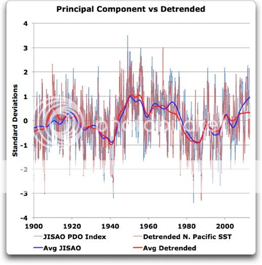
Then, instead of taking the principal components, I simply detrended the result. Here is the comparison, between a simple detrend and the principal component method.
Now, you may recall my statement was as follows:
The actual data shown above is a complete confirmation of my claim. The JISAO PDO Index, calculated as the principal component of the SST data, is indeed quite similar to the simple detrend of the same data (correlation = 0.76). And if I had the actual dataset they used, instead of using the HadISST, the similarity would be even greater.
Both you and Paul have told me, at times in rather unpleasant fashion, that I was misunderstanding the situation … I’ll gladly accept an apology from either or both of you. It turns out that I understood what I was saying very well, and it was you and Paul who were wrong. I may be self-educated, which has its own problems, but as a result I’ve noticed a few things that the professionally trained folks such as you two might have missed in your education …
w.
dp, once tropical storms get heat in to middle upper troposphere a significant amount will be lost to space. Rest goes polewards by Hadley convection.
Warmer SST will radiate all along the path, leaving some residual effect at high latitudes.
there it will melt ice , increase open sea area and increase direct radiative loss to space and increase evaporation.
W. Pacific wind speed reflects SST at the point Willis describes as the splitting of tropical currents to go north and south. Note the 5.42 year peak:
http://climategrog.wordpress.com/?attachment_id=281
The same period of 5.42 years can be found in the rate of change in arctic ice area:
http://climategrog.wordpress.com/2013/03/11/open-mind-or-cowardly-bigot/ddt_arctic_ice/
So, no it’s equal to… there are many ways the heat dissipates, but changes in W. Pacific can be seen reflected in observable data at the pole.
“Both you and Paul have told me, at times in rather unpleasant fashion, that I was misunderstanding the situation … I’ll gladly accept an apology from either or both of you.”
I think I told rather politely that you were misunderstanding the situation. You still are.
The step that you have missed despite have quoted it and spelt it out is the” I subtracted the monthly mean global average SST anomalies, just as the JISAO folks did” bit.
That is where the “something like detrending” comes from not the EOF.
I’ll gladly accept an apology (and thanks for all the time I’ve spent patiently explaining this so that you don’t need to google to find out what EOF is for yourself) 😉
Like I’ve said before , don’t take it the wrong way when I correct some aspect when you get something a bit wrong. You come up with some good stuff and it would be more robust to criticism if you got the maths/physics right. You do most of the time. If I correct you on something it’s to reinforce it, not try to get one over on you because your self-educated.
Most of the important things I know are self taught and I’m pretty much like yourself. When I need to do something , I find out and I do it. I’ve no disrespect for that.
Greg Goodman says:
June 9, 2013 at 3:32 pm
I fear I don’t understand that. I followed their procedures, right up to the point where they calculated the PC and I used the detrend. The results were very similar. You say I missed a step … what step did I miss? Here are the two procedures
THEIR PROCEDURE
Take the N. Pacific SSTs
Subtract the global SSTs
Take the principal components
MY PROCEDURE
Take the N. Pacific SSTs
Subtract the global SSTs
Detrend
The results are very similar … what step am I skipping?
What am I not seeing here? How did I get to something so similar their PC results by using a simple detrend, if (as you and Paul claim) they should not be similar?
Your explanation explains nothing.
w.
@Willis 1:51 pm –
About SABRE: http://www.nasa.gov/topics/earth/features/AGU-SABER.html
Pretty cool stuff. And a perhaps significant step forward, adding an entirely new element to the climate change debate. With a non-constant atmospheric radiation budget, the legs might be knocked out from under current assumptions.
Steve Garcia
Oops! A H/T Eric Eikenberry who pointed all that out to Willis…
Steve Garcia
I did not say you were skipping a step in the processing. I meant you were missing the significance of something you had described doing: ‘The step that you have missed despite have quoted it and spelt it out is the” I subtracted the monthly mean global average SST anomalies” bit’.
You are missing the fact that a step (common to both) is subtracting the global mean, That has a “similar” trend to N.P. data and is effectively detrending it. You’ll probalby find your additional detrending did not make much difference after that.
The EOF is just like a fancy way of getting an average kind of series that is “typical” of the data.
Thanks for your answer Bob and the links. Willis doesn’t seem to be interested in the NOAA 1000 year reconstruction.
Perhaps I’ll try again another day.
Here is a link to the foundational paper on self-organised criticality by Bak, Tang and Weisefeld (“BTW 1987”):
http://webber.physik.uni-freiburg.de/~jeti/studenten_seminar/stud_sem05/bak.pdf
This points to the establishment of attractors in open dissipative systems. The PDO is an example of such an attractor.
In this paper, we argue and demonstrate numerically that dynamical systens with extended spatial degrees of freedom naturally evolve into self-organising critical structures of states which are barely stable. We suggest that this self-organising criticality is the common underlying mechanism behind the phenomena described above. The combination of dynamical minimal stability and spatial scaling leads to a power law for temporal fluctuations. The noise propagates through the scaling structures by means of a “domino” effect upsetting the minimally stable states. Long wavelength perturbations cause a cascade of energy dissipation on all scales, which is the main characteristic of turbulence.
A “power law for temporal fluctuations” in climate demands oscillation on the timescale of the PDO as it does on all timescales.
Eric Eikenberry says:
June 9, 2013 at 11:30 am
“If you’re looking for a controlling “trigger”, the very fact that the atmosphere can and does expand and contract should be considered a major factor. This must have an effect on the jet stream patterns, and by default, the PDO through cloud cover placement due to the jet stream.”
Joule heating of the upper atmosphere apparently causes strong circulation in the polar regions which appears to have a strong influence on the Arctic Oscillation and hence the jet stream, and as you say, the PDO: http://www.arctic.noaa.gov/detect/detection-images/climate-ao_nov-mar_2011-600.png
A complex oscillation with alternating periods dominated statistically (but in a messy sort of way) by high fluctuations (el Nino) and low fluctuations (La Nina) – it looks very like a Lorenz attractor.
As proposed here a couple of years ago.
Ulric Lyons says: “Joule heating of the upper atmosphere apparently causes strong circulation in the polar regions which appears to have a strong influence on the Arctic Oscillation…”
AO leads d/dt(CO2) at Mauna Loa !
http://climategrog.wordpress.com/?attachment_id=227
and d/dt(CO2) correlates with global mean SST :
http://climategrog.wordpress.com/?attachment_id=223
any more specifics on that Joule heating ‘influencing’ AO ? Numbers?
” It turns out that I understood what I was saying very well, and it was you and Paul who were wrong. I may be self-educated, which has its own problems, but as a result I’ve noticed a few things that the professionally trained folks such as you two might have missed in your education …
w.”
… I’ll gladly accept an apology from either or both of you. 😉
Greg Goodman says:
June 9, 2013 at 3:57 pm
I still don’t understand your point. I have done nothing but what they did, up to the point that they extracted the leading PC. At that point, I detrended the data instead of extracting the leading PC … and MY RESULTS ARE VERY, VERY SIMILAR TO THEIR RESULTS.
Which, if you recall, is what I said about the JISAO results, and what you and Paul both said was wrong, wrong, wrong …
You are correct that the final detrending doesn’t do much … but so what? I never said it did. All I required is that the time series end up detrended.
What I said was the following:
I have now tested my claim with the JISAO data. In fact, the two results are indeed quite similar.
So I’d say I was right, that for a slowing trending timeseries, the leading PC is quite similar to the detrended dataset itself. I have actually demonstrated that that is the case for the JISAO analysis, which if you recall was the reason for my comment. So do all the handwaving you want. I have experimental results on my side that show my claim was correct. You can argue about why it was correct all you want.
If you can come up with a different dataset that gives a different result, one where the leading PC of a slowly trending climate time series is greatly different from the detrended dataset, then you can make more claims. Bear in mind that the trend of the N. Pacific SST dataset is only 0.04°C per decade …
So when you come up with some kind of slowly trending timeseries, be it HadCRUT4 global average surface temperature anomalies, N. Pacific average monthly anomalies, or some other timeseries, a timeseries where the leading PC is NOT “quite similar” to the detrended dataset, then we can discuss this more.
But until then, I’ve shown my claim is true by experiment, and you’ve merely proven my point. In fact, the JISAO PDO Index is very similar to the detrended data itself.
w.
PS: From Princeton, regarding Principle Component Analysis, emphasis mine….
Note that that is the same as what I said, which you claimed was wrong:
In other words, the PC analysis involves the rotation of the axes to extract the PCs, just as I said.
Now, the key to what I’m claiming is that if there is only a very small trend in the data, the corresponding amount of axis rotation needed to extract the leading PC is also very small.
And because the result of a very small rotation is quite similar to the result of the removal of a very small trend, for a time series with a small trend (e.g. the global average surface air temperature) detrending is quite similar to extracting the leading PC … which is what I said about the JISAO PDO Index to start this off, and which is what I’ve just demonstrated with the JISAO PDO Index.
PPS: the reason that rotation by a small angle is equal to removal of a small trend is that for small angles, Tan(a) ≈ a. So removing a trend (which is Tan(a)) has nearly the same effect as a rotation by “a”. They are not identical, because trend removal is a shear transformation, and extracting the PC is a rotation. But they are quite similar.
No time for the personal crap — total waste of time.
Reminder:
http://www.billhowell.ca/Paul%20L%20Vaughan/Vaughan%20120324%20Solar-Terrestrial%20Resonance,%20Climate%20Shifts,%20&%20the%20Chandler%20Wobble%20Phase%20Reversal.pdf
More info on this for those who appear to need more than what’s minimally necessary:
http://img268.imageshack.us/img268/8272/sjev911.png
Phase units are pi radians.
[snip Paul – you don’t get to set the rules about how discussion will “advance” on my website. Feel free to resubmit sans that “personal crap”.- Anthony]
Paul Vaughan says:
June 9, 2013 at 8:13 pm
Translation: you’ve been shown to be wrong, and are unwilling to admit it …
w.
Paul Vaughan says:
June 9, 2013 at 8:21 pm
Thanks, Paul … unfortunately, that’s not the information I asked for. I asked how it was that you claim that that plot showed, what was it, hang on … oh, yeah, your claim was that that uncited, unreferenced graph, with no hint of the source of the data, showed that “The changepoints in the integral of NPI are controlled by solar activity & asymmetry”.
Since the changepoints in the integral of the NPI are in 1922, 1945, 1976, and 2005, and those dates are not readily apparent in your mystery graph, I asked what you were talking about … and in response I get an insult, and no new information.
You’re losing ground fast here, my friend.
w.
Henry@Phil.
you confuse E-UV (extreme UV) with F-UV (far UV)
As I understand, the E-UV is what forms the O3, HxOx and NxOx
The more E-UV, the less F-UV and normal UV will be coming through,
due to back radiation of this type of radiation by the increased O3, HxOx and NxOx
so, the less energy is coming into the oceans.
Just remember this: the bulk of earth’s energy from the sun is the warming of the SH oceans,
by the UV coming through. In the SH there is less ozone in the atmosphere….
(how clever is our Creator!)
Thanks, this is the most conceptually helpful article this dilettante has encountered.
Willis: “You are correct that the final detrending doesn’t do much … but so what? I never said it did. ”
“So I’d say I was right, that for a slowing trending timeseries, the leading PC is quite similar to the detrended dataset itself.”
Right ,so you have finally realised the EOF resembled the detrended because the detrending did not matter.. Of course the EOF “resembles” the data, the whole point of doing an EOF is to get something the optimally “resembles” the data.
You are now going argue until the cows come home, I have better things to do.
re. Pautl : “Translation: you’ve been shown to be wrong, and are unwilling to admit it …”
Look in the mirror , my friend.
Greg Goodman says:
June 10, 2013 at 12:16 am
So now you agree with me, that the leading PC resembles the detrended data … but you claim the detrending doesn’t matter. You provide no math and no examples to support this, but that doesn’t matter to you I guess.
You also claim that I agree that “the detrending did not matter”. I said no such thing. I said how the dataset was detrended didn’t matter. As long as it is detrended it will resemble the leading PC.
And now you seem to agree that it is quite similar … so what are you arguing about if you admit my original statement was right?
The better thing to do would be to provide either math or examples to support your argument. I’ve provided both. You’re just taking your ball and going home because you can’t stand losing.
OK, here’s what the mirror shows. I have provided both an example and the math to back up my claim that the detrended version of a dataset with a small trend is quite similar to the leading PC. You now appear to agree, but you dispute my logic … but since you agree that they are quite similar, I don’t see where you have a lot of traction.
The mirror also shows that Paul, like you, hasn’t provided a damn thing except his lip to back up his opinion, which I’ve shown to be wrong by providing both the math and the example and the citation to the paper on Principal Component Analysis. I’ve invited you both to provide a counter-example, or to show where my math is wrong.
Neither of you have provided a damn thing to back up your view. No examples. No citations. No math. I’ve provided all three. Well, to be fair, you’ve done something, so you’re ahead. You re-stated your error several times, but Paul didn’t even do that.
And finally, the mirror shows your back as you go out the door rather than admit your error …
Happy with the mirror-gazing now?
w.
At Anthony’s suggestion I’ve added an integral (cumulative) function to WFT which can partly replicate Willis’ result, but using PDO (which as he explains is inverted to the pressure data he is using). The data must be fairly symmetrical around zero because I haven’t need to detrend it.
http://www.woodfortrees.org/plot/jisao-pdo/integral
I’ll look at adding the pressure data (it looks a sensible format) when I have a bit more time!
Here’s another interesting result, though – the Atlantic (AMO) shows the same bistable oscillation, but lagging by roughly 20 years:
http://www.woodfortrees.org/plot/jisao-pdo/integral/normalise/plot/esrl-amo/integral/normalise
I’ll leave others to explain what AMO is and ponder what that means 🙂
Paul
Willis:”
Note that that is the same as what I said, which you claimed was wrong:
In any case, my understanding, and please correct me if I’m wrong, is that if you zero the “x” and “y” values of your timeseries data, draw the trend line of the dataset, and rotate the dataset around zero by the angle of the trend line, you get the first PC … no? Yes?
”
You said “please correct me if I’m wrong ” so I did.
EOF does NOT detrend the data. You clearly thought it did, so I corrected you.
The axes in the Princeton link are the “axes” in the n-space made by the all the original data time series observations not the y,t axes of the regional mean you are rotatiing or detrending about. You still have not understood what EOF is about but at least you’re starting to read up on it now.
This may help you understand SVD , rotation and orthogonality:
http://www.google.fr/url?sa=t&rct=j&q=&esrc=s&source=web&cd=2&ved=0CDcQFjAB&url=http%3A%2F%2Fwww.ling.ohio-state.edu%2F~kbaker%2Fpubs%2FSingular_Value_Decomposition_Tutorial.pdf&ei=Ho61UYNyqq7RBf_-gagB&usg=AFQjCNGc7F5X3NTJIifUyDKlqZ3p_3o7bQ&bvm=bv.47534661,d.d2k&cad=rja
You are now hiding behind “slowly trending” and trying to confound this with insignificant trend.
Your original text was:
“Current usage seems to favor either the detrended North Pacific temperature, or alternately using the first “principle component” (PC) of that temperature. Since the first PC of a slowly trending time series is approximately the detrended series itself, these are quite similar.”
” the detrended North Pacific temperature” here refers to the regional average temperature, this is what gets detrended. This is not what get used to derive the PC. At that stage you wording implies you thought it was the PC of averaged time series.
If you chose to interpret “slowly trending” to mean negligibly small trend, then what you are noting as being similar is the first PC of the full dataset and the regional mean. Of course they are “similar” in the case where there is negligible trend , the whole point EOF is to get something that is considered to be more representative of a real time series than a regional average.
Both your method and the JISAO processing had identically removed the trend by subtracting the global average beforehand.
So to that extent noting they are “similar” is stating the obvious. It is banal.
All your discussion about centring the data rotating, shear etc. clearly shows that you thought there was some finite trend remaining and the EOF was removing this in a similar way to a simple detrending that you did.
This is where you where wrong and what I was trying explain to improve your understanding. I have now spent a lot more time than it is worth to help one man understand one small point that is not central to the point of this post.
Now since that one man seems more driven by defending his ego that learning the maths, I really have better things to do.
You have produced a valuable result in the cumulative integral of pressure as a Hurst-like detection of regime change, verified by detection of know earlier change points. Clearly identifying 2005 as a new, recent change point in the N. Pacific is a significant result
Congratulations on that result.
Oh, and someone mentioned sunspots:
http://www.woodfortrees.org/plot/sidc-ssn/integral/detrend:160000
Supplementary:
http://imageshack.us/a/img201/4995/sunspotarea.png
Data:
http://solarscience.msfc.nasa.gov/greenwch/sunspot_area.txt
http://solarscience.msfc.nasa.gov/greenwch/sunspot_area_north.txt
http://solarscience.msfc.nasa.gov/greenwch/sunspot_area_south.txt
Frequency changes of the red line here are controlled by the orange line here:
http://tallbloke.files.wordpress.com/2013/03/scd_sst_q.png
Crucial background info:
http://imageshack.us/a/img267/8476/rrankcmz.png
See section 3 here: asymmetric sun viewed from the heliosphere – Mursula (2007)
Regards
Greg Goodman (June 10, 2013 at 1:51 am) addressed Willis:
“You have produced a valuable result in the cumulative integral of pressure as a Hurst-like detection of regime change, verified by detection of know earlier change points. Clearly identifying 2005 as a new, recent change point in the N. Pacific is a significant result
Congratulations on that result.”
The value here is that there are a lot of readers here who will pay attention to this graph when Willis shows it …because it’s Willis showing it and they like Willis socially — not because they independently were able to recognize it as important when it was pointed out many times over the past several years by other WUWT commentators.
This is the second time in a few weeks that Willis has done a re-make of stuff others have shown here in the past. The exposure is welcome. The lack of acknowledgements is informative.
I think you have a point about lack of acknowledgement , I’ve noted that also. However, I’m unaware of anyone else finding such a clear indication of a change point in 2005 by this method or any other.
lgl’s claim to have “done this years ago” did not stand up to scrutiny. Apparently he did something “exactly the same” but difference 18m ago. He used a cumulative integral, did not detrend or remove the average and did not use it to point out regime changes and did not find 2005.
Are you aware of anyone having demonstrated a change point in 2005 anywhere before?
@Paul Clark
/OT
Hi Paul, since you popped in some quick requests:
ICOADS SST , hadley based datasets do funny things to frequency and have huge ‘adjustments’. It would be useful to have the original data available too.
http://climategrog.files.wordpress.com/2013/03/icoad_v_hadsst3_ddt_n_pac_chirp.png
A decent filter option. Running means are an awful choice, though popular.
http://climategrog.wordpress.com/2013/05/19/triple-running-mean-filters/
Gaussian would be nice but triple RM is very good for removing stuff like 12m cycle and would be trivial to add to your site. Just do three running means instead of one. Details in the link above.
Yes, it can be done now but it’s laborious and 99.99% of visitors will just choose from the list. Here’s why it’s needed:
http://www.woodfortrees.org/plot/rss/from:1980/plot/rss/from:1980/mean:60/plot/rss/from:1980/mean:30/mean:22/mean:17
Also is there any way to turn on the grid or at least get a straight line on a plot at y=0 for example?
I have enough knowledge to do all I need with gnuplot locally but a lot of people here seem to like linking stuff on woodfortrees so these few improvements would be helpful, should you be so inclined.
Thanks.
/OT
Greg Goodman says: June 9, 2013 at 11:01 am
” It is NASA, a satellite measured this in 2010.”
You don’t even seem to know what you’re looking at so you are probably drawing the wrong conclusions.
I had a very successful career proving people with PhD’s wrong, so I recognize your ignorant perspective.
With HADISST:
http://i863.photobucket.com/albums/ab195/weschenbach/principalcomponentvsdetrended_zps4f68b37f.jpg
With ERSSTv3b: Not so much.
Greg Goodman (June 10, 2013 at 4:56 am) wrote:
“I think you have a point about lack of acknowledgement , I’ve noted that also. However, I’m unaware of anyone else finding such a clear indication of a change point in 2005 by this method or any other. […] Are you aware of anyone having demonstrated a change point in 2005 anywhere before?”
Yes, this has been appearing in illustrations shared at WUWT for years. You missed it.
The more important point is that any sensible explorer will independently find it within seconds of having the data, so it’s a trivial “discovery”.
Those of us living in the Pacific Northwest experienced the change firsthand.
Finding it in a graph is a trivial exercise, but the change is important.
Important: The changes around 1900 & 2000 are of a different nature than the others. They correspond with 9 year solar asymmetry phase reversals, whereas the others correspond with thresholds in the phase relations of 9 year solar asymmetry and 11 year solar activity. The 9 year solar asymmetry occasionally stretches itself to 13.5 years = 9 + 9/2. The 2 times when it has done this are ~104 to 108 years apart on the record. This is a well-known period of solar activity. Don’t make the mistake of thinking the other changepoints are of the same nature — they’re not.
Can you reproduce section 3 of Mursula (2007) by a number of different methods? You should be able to get the same results with sunspot numbers (not just geomagnetic indices) using a variety of methods. The result is robust across method. Furthermore, the result is extensible to other timescales and this is crucially important to realize.
I’m severely pressed for time — that’s all I have time for today…
Steve Keohane says:
Greg Goodman says: June 9, 2013 at 11:01 am
” It is NASA, a satellite measured this in 2010.”
You don’t even seem to know what you’re looking at so you are probably drawing the wrong conclusions.
I had a very successful career proving people with PhD’s wrong, so I recognize your ignorant perspective.
Congratulations. What has that got to do with anything here? I don’t have a PhD and you didn’t prove me wrong.
Steve, you posted a totally anonymous graph (map plot) with NO information whatsoever, so I asked you what it was. You replied “it is NASA” , no it is not it’s a graph, NASA is a government agency. Then ” a satellite measured this “. Duh, which satellite , there are thousands. Yes NASA have satellites too, getting warmer. You apparently did not reply in an informative manner because you still did not even know what it was you’d posted.
So, yes I am “ignorant” of what it is and remain so because you cannot be arsed to say what it is you expected us to look at . I sure am not going to go on some paper chase trying to guess what it is.
And since you apparently didn’t know what the graph you posted was, it seemed reasonable to suggest you may be drawing the wrong conclusions.
Though I don’t usually get paid for it, I too have a long history of spotting people who don’t know what they are talking about and seeing through paper thin attempts to cover it up.
Shame I don’t get paid for it , I seem to be getting more that my fair share today.
So why did you bring this irrelevancy back into the discussion? Just for the opportunity to be insulting. Very impressive.
PV: The more important point is that any sensible explorer will independently find it within seconds of having the data, so it’s a trivial “discovery”.
Since it is so trivial and so obvious and everyone who ever picked up a dataset must obviously have found this “within seconds” probably accounts for why no one is able to point to where it has been shown already: it so obviously and trivial that no one ever thought it was worth mentioning.
Yeah, that must be it.
[ Greg, just a quick note to say here’s how to get a y=0 line:
http://www.woodfortrees.org/plot/jisao-pdo/integral/plot/jisao-pdo/scale
The rest, as my University computer support team, used to say, “Noted” 🙂 ]
Willis, if what you say is true, that the PDO is a temperature regulating mechanism, then I would not expect that there is good correlation between PDO and temperature. That’s because generally the better the regulator the smaller the correlation with the regulated effect. A perfect regulator would have zero correlation.
(Paul Clark) says:
[ Greg, just a quick note to say here’s how to get a y=0 line:
http://www.woodfortrees.org/plot/jisao-pdo/integral/plot/jisao-pdo/scale
The rest, as my University computer support team, used to say, “Noted” 🙂 ]
Thanks for the tip, that does at least provide a reference for looking at rate of change +ve or -ve.
I hope you will find time to add some of the other things I mentioned.
thx.
Dan Evans, that’s a very good point to make. I’m all for Willis’ TS “governor” except that I think it’s more powerful than a governor, though that’s a good staring point.
However, I don’t think PDO is regulation , it is a measure of the controlled variable. Using NPI is a good idea. I don’t have any time for PDO or AMO, both “detrended” indices since there is not such thing as a linear “trend” in climate to be measured and subtracted. This is all borne of the failed hypothesis of a linear response to exponentially increasing CO2. This is essentially what they imagine they are splitting out.
To fit a linear trend you need to have a model that includes a linear trend. The a priori assumption for the last 30 years has be linear CO2 response + noise.
That model has failed and the recent volcano stack analysis proves it dead in the water.
Without the linear response there is no justification for linear “detrending” and thus AMO and PDO , as detrended indices, go out the window too.
If someone wants to suggest a slow rise sicne LIA we need to know what it really is before we can approximate it. ie where it tops out before we can use a linear as an approximation for that.
Now if we can free ourselves from all this baggage of preconcieved assumptions we may start to see what climate really does.
The lowest NPI monthly value each year is not always in January, and often correlates to the most negative monthly NAO value, suggesting a common driver:
http://snag.gy/OWNEs.jpg (NPI 1899.01 to 1948.12)
http://climatedataguide.ucar.edu/sites/default/files/cas_data_files/asphilli/npindex_monthly_1.txt
http://climatedataguide.ucar.edu/sites/default/files/cas_data_files/asphilli/nao_station_monthly_2.txt
“This discussion of pressure-based indices makes me think that there should be some way to use pressure as a proxy for the temperature.”
Compo et al 2013 did something similar. Bob covered this here:
http://wattsupwiththat.com/2013/04/08/a-preliminary-look-at-compo-et-al-2013/
“We use a completely different approach to investigate global land warming over the 20th century. We have ignored all air temperature observations and instead inferred them from observations of barometric pressure, sea surface temperature, and sea-ice concentration using a physically-based data assimilation system called the 20th Century Reanalysis.”
http://www.woodfortrees.org/plot/rss/from:1980/derivative/mean:12/mean:9/mean:7/plot/hadcrut3gl/from:1980/derivative/mean:12/mean:9/mean:7/plot/rss/scale/from:1980
Thanks to Paul Clark’s tip here’s rate of change of two surface temp series. Using the eye to ignore the bumps, it seems rate of change crossed from +ve to -ve in… 2005.
Paul C.
Thanks for adding the integral to w43s, long missed.
http://www.woodfortrees.org/plot/jisao-pdo/from:1900/normalise/integral/detrend:-10/normalise/plot/hadsst3gl/from:1900/mean:90/detrend:0.6/normalise
The integral of AMO does not make much sense since AMO is already the integral of ENSO,
http://virakkraft.com/Nino34-AMO-deriv.png (or maybe the AMO integral will anti-correlate arctic sea ice)
Remember where you saw it first Greg. (yes it’s exactly the same as Bob has been telling for years, just different 🙂
greg goodman says
http://wattsupwiththat.com/2013/06/08/decadal-oscillations-of-the-pacific-kind/#comment-1331971
henry says
from what time onward did we lose the idea of putting the (SI or other) dimension on the scale of the y-axis,
like I put in here?
http://blogs.24.com/henryp/2012/10/02/best-sine-wave-fit-for-the-drop-in-global-maximum-temperatures/
I’ve just found the pattern that I got from the volcano stack. Spotted it in RSS
http://www.woodfortrees.org/plot/hadcrut3gl/from:1980/derivative/mean:12/mean:9/mean:7/plot/rss/scale/from:1980/plot/hadcrut3gl/derivative/mean:24/mean:17/mean:13/from:1983/to:2000
cf
http://climategrog.wordpress.com/?attachment_id=278
Now I’d already notices that the bumps looked like a full wave rectified (magnitude) cosine and that there were damn near four cycles in the 11 year interval between the higher peaks This suggests 11/4 or 11/2 as the the underlying cosine.
Looking at the RSS plot I realised it is two cosines added 11/3 and 11/2 = 3.7 and 5.5 years. In view of the crudity of this calculation, that’s the same as is found in W. Pacific wind speed.
http://climategrog.wordpress.com/?attachment_id=281
Now those two are mathematically equivalent to 2/(3/11+2/11) modulated by 2/(3/11-2/11) = 4.4 and 22 years
4.4 is very close to 8.85/2 =4.425 years, half the lunar aspides cycle. 22 years does not need any introduction.
Willis’ demonstration of the importance of tropics as general climate regulator explains the halving of that period. (cf sun passes over twice a year giving a strong six monthly signal).
The volcano stack shows that major eruptions synchronise with this sequence often enough for it to be the dominant pattern when they are averages together. So there’s a luni-solar link to the timing of those eruptions too.
Wow.
Thanks to Stuecker et al from drawing my attention to W. Pacific winds and to Willis for the idea of stacking volcanoes.
HenryP says:
June 9, 2013 at 11:29 pm
Henry@Phil.
you confuse E-UV (extreme UV) with F-UV (far UV)
No I don’t!
The ISO standard on determining solar irradiances (ISO-21348)[6] describes the following ranges:
Ultraviolet UV 400 – 100 nm 3.10 – 12.4 eV
Ultraviolet A UVA 400 – 315 nm 3.10 – 3.94 eV
Ultraviolet B UVB 315 – 280 nm 3.94 – 4.43 eV
Ultraviolet C UVC 280 – 100 nm 4.43 – 12.4 eV
Near Ultraviolet NUV 400 – 300 nm 3.10 – 4.13 eV
Middle Ultraviolet MUV 300 – 200 nm 4.13 – 6.20 eV
Far Ultraviolet FUV 200 – 122 nm 6.20 – 10.16 eV
Extreme Ultraviolet EUV 121 – 10 nm 10.25 – 124 eV
O2 absorbs by and is photo-dissociated into 2O by UV shorter than 242nm, i.e. UVC, F-UV and some E-UV.
O3 absorbs by and is photo-dissociated into O+O2 by UV shorter than 310nm, i.e. UVB & UVC
Because O2 and O3 can both absorb short wavelength UV radiation, no solar radiation with wavelengths less than 290 nm penetrates below the stratosphere.
As I understand, the E-UV is what forms the O3, HxOx and NxOx
The more E-UV, the less F-UV and normal UV will be coming through,
due to back radiation of this type of radiation by the increased O3, HxOx and NxOx
so, the less energy is coming into the oceans.
This is completely wrong, also since both O2 and O3 photo-dissociate there is no back radiation of UV, it ends up as kinetic energy, i.e. heat.
Greg Goodman says:
June 10, 2013 at 1:51 am
Gosh, Greg, if I had actually said that EOF detrends the data, you might actually have a point, and all of your succeeding rambling might have gone somewhere useful.
Unfortunately, I never said any such thing. Find me where I said “the EOF detrends the data” or anything like that. That’s just your fantasy. Provide a quote if you think it’s true.
Man, if you could read, you’d be dangerous. As it is, you’re just funny. I can defend my own statements. I can’t defend your fantasies about what I’ve said.
w.
woodfortrees (Paul Clark) says:
June 10, 2013 at 1:45 am
Fascinating, Paul. I can’t even begin to imagine what the dynamics might be in that relationship.
w.
Paul Vaughan says:
June 10, 2013 at 3:29 am
Paul, first, an actual citation to whatever previous work shows the same result that I have found would be good.
Why would it be good?
Because you’ve shown your word to be worthless, and so far all you’ve given me in support of your accusation of plagiarism is your big mouth.
You claim that the method I used, and the identification of the 2005 changepoint, is a “re-make of stuff others have shown here in the past”, and that it has been “pointed out many times over the last several years”.
That is a slimy accusation of plagiarism, Paul, without a scrap of evidence to back it up.
Typical of your bottom-feeding methods …
So here’s your ethical choices. You can either give us the citation to the “many times” that this finding or this method has been pointed out here on WUWT and show that I have stolen their ideas, or you can apologize for your untrue and baseless accusation.
However, you’ll likely take the unethical choice …
w.
Greg Goodman says:
June 10, 2013 at 8:38 am
Greg, I’d somehow missed your volcano stack post regarding SST. Nice stuff, well done.
w.
From Greg Goodman on June 10, 2013 at 8:38 am:
The only “RSS” there is a zero line. It shows you’ve applied your “special sauce” thrice-applied running means to show how well HADCRUT3gl can match HADCRUT3gl.
But it does highlight how much information your “special sauce” loses, distorting shape and amplitude, until the only trustworthy info it imparts for curve-matching is whether a lobe is pointing up or down.
I also noticed how you suppressed the range on the last plot element, when you also take that from 1980 to present it dramatically shows how the “special sauce” will screw up the same data until the curves stop matching, although it is the same underlying data. You have indeed discovered a great tool for finding a desired curve match.
Greg Goodman says:
June 10, 2013 at 4:56 am
So you’re willing to make accusations of plagiarism without providing a shred of evidence, just like Paul … nice.
Back it up or take it back, there’s a good fellow. I do my best to acknowledge all my sources, and have cited comments as touching off my posts.
w.
lgl says:
June 10, 2013 at 8:16 am
lgl, I don’t understand this at all, and the graph you cite doesn’t clarify. How exactly is the AMO the integral of ENSO?
w.
Paul Vaughan says:
June 10, 2013 at 5:28 am
Thanks, Paul. That’s no surprise, because the dataset that they used is some Hadley product. That’s why I used HadISST. I’d probably get closer with HadSST3. Unfortunately, all the website says is:
I think that they are referring to the now-deprecated UK SST product, but I haven’t had time or the interest to do the full analysis. The dataset is only available in gridded form. It is in four blocks in some text format.
I may redo the analysis using HadSST and Reynolds OI data … actually, as I recall the HadSST uses Reynolds OI data, so the HadSST dataset might do it on its own.
Always more to learn,
w.
henry@woodfortrees
Please explain to me as to why the y-axis does not show the dimensions (SI unit or other)
kakada says:
From Greg Goodman on June 10, 2013 at 8:38 am:
I’ve just found the pattern that I got from the volcano stack. Spotted it in RSS
http://www.woodfortrees.org/plot/hadcrut3gl/from:1980/derivative/mean:12/mean:9/mean:7/plot/rss/scale/from:1980/plot/hadcrut3gl/derivative/mean:24/mean:17/mean:13/from:1983/to:2000
The only “RSS” there is a zero line. It shows you’ve applied your “special sauce” thrice-applied running means to show how well HADCRUT3gl can match HADCRUT3gl.
But it does highlight how much information your “special sauce” loses, distorting shape and amplitude, until the only trustworthy info it imparts for curve-matching is whether a lobe is pointing up or down.
I also noticed how you suppressed the range on the last plot element, when you also take that from 1980 to present it dramatically shows how the “special sauce” will screw up the same data until the curves stop matching, although it is the same underlying data. You have indeed discovered a great tool for finding a desired curve match.
===
Well spotted, I retained hadcrut instead of RSS. Immaterial to the point of what I found.
RSS is there as the work around to get a straight line out of woodfortrees that the owner provided me with earlier. Messy but it seems the only way get a zero line and there’s no grid available on his plots.
If you have some intelligent objection to the triple running mean I’m very interested. Calling it a silly name does not impress me. If you read my page on why the filter is used you may learn something.
http://climategrog.wordpress.com/2013/05/19/triple-running-mean-filters/
“But it does highlight how much information your “special sauce” loses, distorting shape and amplitude,…”
That’s called filtering genius.
I limited the range to be about the same as what I used in the volcano stack plot. No underhand or special sauce reasons. Perhaps you’d like to replicate the volcano stack,run it back to 1980 and post back with a relevant comment.
On the other hand you can carry on making ill-informed, uneducated snipey remarks as usual. Seems to be about the limit of you intellect as evidenced so far.
Phil. says
O2 absorbs by and is photo-dissociated into 2O by UV shorter than 242nm, i.e. UVC, F-UV and some E-UV.
Henry says
some?
papers?
proof?
lgl says:
The integral of AMO does not make much sense since AMO is already the integral of ENSO,
http://virakkraft.com/Nino34-AMO-deriv.png (or maybe the AMO integral will anti-correlate arctic sea ice)
Here is d/dt sea ice against SST , both the derivative of what you were suggesting, so similar comparison. Long term the two run together but the dominant period in AMO does not match ice.
http://climategrog.wordpress.com/?attachment_id=160
However, that’s two more data sets showing a change of behaviour around 2005.
Willis
ENSO~AMO derivative, then ENSO Integral~AMO
A bit off in the 50s so add some NAO.
Willis, Degree or not, you are are an engineer’s engineer.
lgl says June 9, 2013 at 8:15 am, referring to Bob Tisdale:
“This recharges (or replenishes) the heat released during the El Niño.”
Oh not that nonsense again. El Niño heats the tropical Pacific, http://virakkraft.com/Rad-Temp-Trop-Pac.png
The graph you ar linking to I guess show SST combined with downward radiation, and of course showing that SST is higher during El Niñjo than during La Nina. As I understand Bob Tisdale he would not disagree with that. But when this heat enters the ocean is quite another matter, as this happens during a La Nina directly by the sun from a clear sky, gradually as the surface water is transported by the trade winds westward. And then it ends up in the West Pacific, warmer and reaching far deeper as it batters up. During an El Niñjo it sloshes back and spread out over the surface all the way to South Amercica, resulting in higher SST and releasing much of the heat to the atmosphere. So there is indeed a time scale combinded with some pure physical phenomena to be taken into consideration here in order to grasp the mechanism. That is what Tisdale very thorougly explains in this video as far as I understand him:
A time to time presumed relation between mean downwelling radiation and SST seems to miss the actual phenomenon.
Or dou you mean that the ocean heats more from backradiation from clouds During El Niñjo than from from a direct sun in a clear sky during La Nina?
From Greg Goodman on June 10, 2013 at 11:12 am:
Long range weather forecasting is farmer business but a gamble.
In Rhodesia in the 70s we used El Nino and the winter rainfall in the South African Cape as an indicator for a dry summer and an option to use wet land for planting maize in an attempt to minimize the financial risk. Alexander has lots to say on the subject. Willis has his feet on the ground.
Trond A
2/3 of the total downward radiation is LW, all the time.
lgl
Your answer is short as usual 🙂
A bit less than that if you use mean values as 161 W/m^2 hitting the ground directly from the sun and totally 390 W/m^2 (calculated from the surface (also calculated) mean temperature of the earth as 15C) because of added LW backradiation. But if you try this relation out on a tropical desert with the incoming radiation from a zenith sun I am afraid it will get terribly hot, maybe twice or more than ever experienced.
I guess I’ll have to interpret your answer in the way that you don’t agree with the described mechanism of warming during La Nina from a direct sun, but that LW radiation heats the ocean more effectively(?).
1) Here I linked to my own graphs of several climate index integrals — including NPI:
http://wattsupwiththat.com/2009/12/21/hansen-on-the-surface-temperature-record-climategate-solar-and-el-nino/#comment-271900
2) Here I showed the integral of -NPI on both pages 21 & 22:
http://wattsupwiththat.files.wordpress.com/2011/10/vaughn-sun-earth-moon-harmonies-beats-biases.pdf
3) Above I shared a reminder — anyone who linked to that reminder saw a graph of the integral of -NPI featured prominently on p. 1:
http://www.billhowell.ca/Paul%20L%20Vaughan/Vaughan%20120324%20Solar-Terrestrial%20Resonance,%20Climate%20Shifts,%20&%20the%20Chandler%20Wobble%20Phase%20Reversal.pdf
Plenty of other people will have the NPI integral on file. It’s routine to do a graph like that when looking at a new series. Just like we don’t cite hundreds of other people who’ve smoothed a time series when we smooth the same time series, we don’t need to cite other people who have looked at an integral. What I objected to here was comically obsequious commentary attempting to make it appear that Willis had pioneered some heroic breakthrough by trivially plotting the NPI integral.
Trond A (June 10, 2013 at 2:21 pm) wrote:
”
lgl
Your answer is short as usual 🙂
“
lgl is a model commentator — concise and focused sharply on tearing down boundaries at the knowledge frontier.
HenryP says:
June 10, 2013 at 11:25 am
Phil. says
O2 absorbs by and is photo-dissociated into 2O by UV shorter than 242nm, i.e. UVC, F-UV and some E-UV.
Henry says
some?
papers?
proof?
Plenty, now read some, I can provide many more if you wish.
http://rstb.royalsocietypublishing.org/content/361/1469/769.full
http://www.ccpo.odu.edu/~lizsmith/SEES/ozone/class/Chap_5/5_2.htm
lgl says June 9, 2013 at 8:15 am, referring to Bob Tisdale:
“This recharges (or replenishes) the heat released during the El Niño.”
Oh not that nonsense again. El Niño heats the tropical Pacific, http://virakkraft.com/Rad-Temp-Trop-Pac.png
lgl, that plot shows a strong correlation with _something_. Is there any chance you could make it into a meaningful graph by explaining _exactly_ what is being plotted.
we now know that DW mean downwards radiation but is this SW,LW, total , TOA, surface, global mean , Pacific. ????
Temp for tropical Pacific is what? Air, SST, which region? nino3.4 all tropics.
A graph like that means _nothing_ to anyone except he who plotted it and knows what the data was.
Now there’s a strong correlation there which may either confirm or refute certain ideas. If you have a point to make how about posting that graph which properly labelled axes and preferably references to data sources so we can reproduce it?
BTW my brain is a bit slow at dividing by 12 and adding 1980, how about a proper x axis that I don’t have to do mental gymnastics to read?
You seem to think it’s important (and you may be right) so how about communicating it in a useful form.
Willis concludes: „As a result, it makes perfect sense and is in accordance with the Constructal Law that when the sea temperature gradient from the tropics to the poles gets steep enough, the ocean currents will re-organize in a manner that increases the polewards heat flow. Conversely, when enough heat is moved polewards and the tropics-to-poles heat gradient decreases, the currents will return to their previous configuration. But exactly what those reversal thresholds might be, and when we will strike the next one, remains unknown.”
To predict the global climate one has to separate the effects of the Sun, which gives the heat load power, from the effects of the oscillating Earth, which are generated from the Earth axis wobble of about 433 days (s. my above posting).
It is clear, that an oscillating Earth axis, coupled to the QBO oscillation of the atmosphere wit 2 times 433 days or 2.366 years, and coupled with the ENSO Oscillations of 3.55 years as a sub harmonic main mode 3 besides other ENSO frequency modes cannot lead to prediction of the global temperature for longer than a year, because in that impedance of the ocean oscillations no heat is created; the heat load frequencies for longer and for shorter time than a year coming from the Sun only.
Solving the problem of separating both effects, it helps to remove the ENSO function from the global temperature record function, because the remaining function then is the heat load function from the Sun (Red curve). The remaining function can now compared with the heat load generating function of the Sun (Blue curve).
http://www.volker-doormann.org/images/enso_removed.gif
From this mathematics and the correlation of time coherence it is evident that the ignored global temperature frequencies of Earth wobble (ENSO) and Sun tides are the basis of the nature of terrestrial climate.
It seems, that the known basis of the ENSO function as generated from the Earth wobble frequency of 433 days, can be solved and synthesised. This would open the door to a precise global temperature prediction.
However, hints of this kind are blowing in the wind …
V.
lgl, first you quoted me out of context and without attribution, “This recharges (or replenishes) the heat released during the El Niño.” The full paragraph reads:
The recharge of ocean heat in the tropical Pacific during a La Niña is a function of cloud cover and sunlight. Because there is less evaporation during a La Niña, there is less cloud cover. Less cloud cover means more sunlight can enter and warm the tropical Pacific. This recharges (or replenishes) the heat released during the El Niño.
And then, lgl, you said, “Oh not that nonsense again. El Niño heats the tropical Pacific, http://virakkraft.com/Rad-Temp-Trop-Pac.png”
Nonsense? Your grasp of reality is somewhat skewed, lgl. You must be hanging out at SkepticalScience again. Your graph also confirms that downward longwave radiation can’t recharge the heat released by the El Niño—in other words, it contradicts the argument you’re trying (and failing) to make.
I assume the “DW Rad.” you’re showing in your graph is downward longwave radiation. Downward longwave radiation increases in the tropical Pacific during an El Niño because the sea surface temperatures are warmer. And the sea surface temperatures are warmer because warm waters from the surface and below the surface of the west Pacific Warm Pool have sloshed to the east. Some of the increase in downward longwave radiation is caused by the resulting increase in the air temperatures of the tropical Pacific. And some of the increase in downward longwave radiation is caused by the increase in cloud cover caused by the increase in evaporation. All in all, the variations in downward longwave radiation are caused by ENSO.
And with your graph, we can see that downward longwave radiation decreases during La Niñas. If the downward longwave radiation decreases during a La Niña, how then could it be the medium that recharges or replenishes the heat released during an El Niño? It can’t. I’ll repeat my earlier comment:
The recharge of ocean heat in the tropical Pacific during a La Niña is a function of cloud cover and sunlight. Because there is less evaporation during a La Niña, there is less cloud cover. Less cloud cover means more sunlight can enter and warm the tropical Pacific. This recharges (or replenishes) the heat released during the El Niño.
And here’s a comparison graph of downward longwave and shortwave radiation for the tropical Pacific:
http://bobtisdale.files.wordpress.com/2013/06/figure-23.png
Sure does look like downward shortwave radiation (sunlight) increases during La Niñas.
That graph is Figure 23 from this post:
http://bobtisdale.wordpress.com/2013/06/04/open-letter-to-the-royal-meteorological-society-regarding-dr-trenberths-article-has-global-warming-stalled/
I described the ENSO processes that cause the relationships between downward longwave and shortwave radiation in detail in that post. See the second paragraph after Figure 22. And I know you at least looked at the graphs in that post because you commented on the thread of the WUWT cross post:
http://wattsupwiththat.com/2013/06/04/open-letter-to-the-royal-meteorological-society-regarding-dr-trenberths-article-has-global-warming-stalled/#comment-1326041
One last thing: What’s the source of the data in your graph? Your “DW Rad.” data appears a bit high, by about 200 watts/m^2.
Tisdale,
You can just give up on trying to teach lgl anything about reality. He’s contained within his own little bubble and have no intention of leaving it, just switching endlessly from one talking point to the next as one proves his last one wrong.
“I am using “throughput” to mean the rate at which heat is moved from the equator to the poles. When the movement of heat to the poles slows, heat builds up. And when that pole-bound movement speeds up, the heat content of the planet is reduced through increased heat loss at the poles.
The rate of throughput of heat from the tropics to the poles is controlled at different time scales by different phenomena.”
In the elaboration decadal ( http://imageshack.us/a/img202/4641/lodjev.png ) was notably skipped and multidecadal (what I’ve called “multidecadal solar throttling of aggregate meridional equator-pole heat & water pumping”) was mislabeled as decadal — see visual summaries I’ve volunteered along with concise notes here:
http://www.billhowell.ca/Paul%20L%20Vaughan/Vaughan%20130224%20-%20Solar%20Terrestrial%20Volatility%20Waves.pdf
With one powerfully concise image, Wyatt, Kravtsov, & Tsonis reminded us to step back from tangles of integrals & derivatives of coupled temperature, mass, & velocity to see holistically:
https://pantherfile.uwm.edu/kravtsov/www/downloads/Presentations2010-2011/AMO_AGU10.pdf
Interpretive Caution:
Their attribution is misplaced. AMO/AMOC = locally amplified manifestation (not driver).
The phenomenon is global and externally governed:
http://tallbloke.files.wordpress.com/2013/03/scd_sst_q.png
Interpretive Caution:
Temporal cycle acceleration/deceleration indicates spatiotemporal acceleration/deceleration more generally due to a simple relationship:
http://iopscience.iop.org/0004-637X/589/1/665/fulltext/57538.fg2.html
… so temporal solar cycle acceleration/deceleration is a proxy for solar spatial pattern change acceleration/deceleration and all related heliospheric spatiotemporal modulation.
This observation challenges us to explore synchronization of gradients (and hence flows) on stars, in heliospheric structures more generally, and on planetary surfaces.
Greg
I’ve told you all you need to know. Downward radiation to the surface, and radiation is total, SW+LW, if not stated otherwise, and I’m sure you recognised the ENSO pattern immediately.
Bob
SW anomaly was positive most of the time 1991 to 2006, when ENSO was also mostly positive.
SW has decreased significantly after 2005, same has ENSO.
Cloud cover has increased a lot since 1995, when ENSO has dropped.
Willis recently showed the upper 100 meters closely follows the surface temps, so your funny notion that LW does not heat below a few millimeters is just – funny. 200 W/m2 solar can’t keep tens of meters of waterdepth at 300 K.
Again, the rule is, the total radiation to the surface, the energy input, is above average when ENSO is above average.
Reality is broader than the single Nino and Nina.
Trond
This should answer your question.
… or maybe I should have said PDO/-NPI instead of ENSO …
Compare SW in 1998-2000 with 2010-2012. Much lower now when PDO is in negative phase, coincidence?
lgl,
The atmosphere is not a second heat source for the ocean surface. That’s why you can not ADD an inferred LW radiation flux to the solar SW radiative heat flux. Radiation is not in itself heat. There is no extra radiative heat coming down to the surface from the atmosphere. The radiative heat flux between surface and atmosphere goes UP. The Sun is the ocean’s only heat source from above.
Like Tisdale said, SST increases first, the surface in turn heats the atmosphere above it, which thus becomes warmer and hence more DWIR can be inferred (notice, it is not measured, merely calculated, the only thing actually being measured is the heat flux – and it goes up). You’ve got it all backwards …
A couple of comments:
1) As for noticing the 2005 change … I’ve been pointing this out of several months after I produced this graph,
http://www.woodfortrees.org/plot/rss/from:1996.8/to/plot/rss/from:1996.8/to/trend/plot/rss/from:1996.8/to:2005/trend/plot/rss/from:2005/to/trend
The reason I came up with 2005 is that is an ENSO neutral year with the best match of a change from a positive trend to a negative one. No, it is not scientific, it is just something I noticed. However, I only posted this chart recently on WUWT. I’ve referenced it at other sites where I’ve been debating true believers by informing them of the great correlation of the PDO with temperatures for the last 100 years. It doesn’t take anything away from the work Willis has done, but Paul V. is also correct in what he stated.
2) I’ve also noticed something about the AMO that may be helpful. It appears to have it’s upward period (from max negative to max positive) and downward period in correlation with the PDO crossing the zero line. In other words, when the PDO becomes positive the AMO starts rising and when the PDO becomes negative the AMO starts dropping (on average). Maybe someone can put some more meat on the bones.
3) Paul Clark … thank you very much for you contribution to climate discussions. I don’t know what I would do without woodfortrees. You should get some kind of award.
lgl says:
June 11, 2013 at 7:29 am
Greg
I’ve told you all you need to know. Downward radiation to the surface, and radiation is total, SW+LW, if not stated otherwise, and I’m sure you recognised the ENSO pattern immediately.
No you have not. And you still refuse to say what you have plotted for some obscure reason.
Bob Tisdale says:
I assume the “DW Rad.” you’re showing in your graph is downward longwave radiation. Downward longwave radiation increases in the tropical Pacific during an El Niño because the sea surface temperatures are warmer.
Why _assume_ anything? If the guy can not even be arsed to say what he is plotting, just ignore it. I for one am not interested is guessing what it may be and then trying to interpret what it may or may not mean.
If he wants to say your work is “nonsense” , without even having the good manners to refer to you directly, he’d damned well better come up with something coherent and at least learn to label a graph so that it is meaningful.
With his Mickey Mouse graph and comments like – AMO, well add a bit of NAO – he is really just posting meaningless drivel.
I would demand that he posted something meaningful before feeling the need to defend yourself. You can’t answer someone who is incapable of showing their basic arguments, so don’t try.
Kristian
I’m not going to discuss that skydragon nonsense. The LW is measured every day around the world. You can’t explain the high temps of the surface without it, for instance 300 K in tropical Pacific and only 200 W/m2 solar input. What’s the temperature of a black-body emitting 200 W/m2? (or make that 60 W/m2 if you like because there is also 140 W/m2 latent transfer)
Richard M. “2) I’ve also noticed something about the AMO that may be helpful. It appears to have it’s upward period (from max negative to max positive) and downward period in correlati2) I’ve also noticed something about the AMO that may be helpful. It appears to have it’s upward period (from max negative to max positive) and downward period in correlation with the PDO crossing the zero line. In other words, when the PDO becomes positive the AMO starts rising and when the PDO becomes negative the AMO starts dropping (on average). Maybe someone can put some more meat on the bones.
on with the PDO crossing the zero line. In other words, when the PDO becomes positive the AMO starts rising and when the PDO becomes negative the AMO starts dropping (on average). Maybe someone can put some more meat on the bones.”
I started looking at cross-correlation of N.Pacific and N. Atlantic SST last year and it was very interesting how the two played off against each other.
…. until I realised that none of what I saw was in the original ICOADS data and was infact an artefact of HadSST3 processing.
At that point I resolved to stop using Hadley data “products” for any kind of spectral analysis and cross correlation work.
AMO is not hadley based but ERSST, but they adopt many of the hadley “corrections”.
http://climategrog.files.wordpress.com/2013/03/icoad_v_hadsst3_ddt_n_pac_chirp.png
This is not sampling “corrections” , their data processing is doing some (apparently unintentional) frequency adjustments.
Also AMO is “detrended” whatever that means is subjectively linked to the assumption that there is a linear trend to be removed, and PDO is the invserse of NP SST minus the global mean and then some EOF magic.
After all that , if there is some relationship between the two I’d be hard pressed to accord it any physical meaning.
IIRC, when I looked at ICAOADS SST all the interplay implied in the cross-correlations disappeared.
Greg
When I’m writing downward radiation without specifying any wavelength, what else than all wavelengths would that be? Why would it be only LW or only SW? Why wouldn’t I say LW if that was what I was graphing?
Richard
“when the PDO becomes positive the AMO starts rising and when the PDO becomes negative the AMO starts dropping”
Just like it is supposed to if AMO is the integral of PDO (or ENSO)
http://www.woodfortrees.org/plot/jisao-pdo/from:1900/normalise/integral/detrend:-10/normalise/plot/esrl-amo/from:1900/mean:90/normalise
Then Greg, add or remove some NAO integral. Temps of the north atlantic is of course also influenced by what’s happening in the north atlantic, so nothing wrong with that.
Phil. says
Phil. says
O2 absorbs by and is photo-dissociated into 2O by UV shorter than 242nm, i.e. UVC, F-UV and some E-UV.
Henry asked:
some?
papers?
proof?
Phil. says
Plenty, now read some, I can provide many more if you wish.
http://www.ccpo.odu.edu/~lizsmith/SEES/ozone/class/Chap_5/5_2.htm
Henry@Phil.
I quote from the above paper that you quoted to me:
……..the Chapman reactions. He proposed that atomic oxygen is formed by the splitting (dissociation) of O2 by high energy ultraviolet photons (i.e., packets of light energy with wavelengths shorter than 242 nanometers) via
O2 + hc/ y–> O + O
Where h is the Planck constant, c is the speed of light, and y is the wavelength of the photon, given in nanometers (abbreviated nm, where 1 nm=10-9 meter). Collectively, hc/y represents the photon of light that breaks up the O2 molecule. The top panel of Figure 5.01 displays the absorption cross section for oxygen multiplied by 10,000. The cross-section is proportional to the probability that a photon from the Sun will be absorbed by an oxygen molecule. While this probability increases for the shorter, more energetic photons, the amount of UV radiation with wavelength shorter than 242 nm reaching into the atmosphere falls dramatically with decreasing altitude.
end quote
While this probability increases for the shorter, more energetic photons
end quote again
now,
as I was saying,
\not “some” (which is what you suggested) but most, if not all, of the E-UV is used to convert oxygen into ozone and HO into HxOx and NO into NxOx at the TOA. The atmosphere protects us from the E-UV. When the sun is quiet, (less SSN) you get more E-UV. More ozone and others TOA means more UV (all types) being back radiated, and less UV coming through the atmosphere. . It is the UV, mostly, that fires up the oceans. If you do not get that bit right, you miss all the fun.
http://blogs.24.com/henryp/2012/10/02/best-sine-wave-fit-for-the-drop-in-global-maximum-temperatures/
now look up when ozone started declining and when it started increasing again both SH and NH and compare that to my graph quoted above??
Have a nice day, Phil.
lgl says, June 11, 2013 at 8:43 am:
“I’m not going to discuss that skydragon nonsense.”
Sorry, but this is not ‘skydragon nonsense’, lgl. I’m simply telling you that the atmosphere is not a second heat source for the ocean. So you cannot add a DWIR flux from the atmosphere, which is not a radiative heat flux, to the solar flux, which is a radiative heat flux. Apples and oranges. If anything, the DWIR is subtracted from the UWIR from the surface (you know, your ‘reduced radiative cooling’). The radiative heat (you know, what you would call ‘the net’) flux between surface and atmosphere goes up. Do you seriously disagree with these facts?
What you need to do is look at the total net air/sea flux at the tropical Pacific Ocean surface and see when the most heat and when the least heat goes into the ocean. I can assure you that you will find that during La Niña or neutral conditions more heat is absorbed by the ocean and that considerably less is absorbed during El Niño conditions – the stronger the event, the less net gain of heat:
http://i1172.photobucket.com/albums/r565/Keyell/Pacificair-seaflux_zpsf8421585.png
Total net air/sea flux is ‘net solar’ (positive) + ‘latent heat’ (negative) + ‘sensible heat’ (negative) + ‘thermal radiation (IR)’ (negative). Notice how the tropical Pacific always gains heat, only to a greater or lesser degree. The swings are really much larger than rendered here, since the curve is smoothed to eliminate the seasonal cycle. The one (and very significant) heat transfer mechanism that must be considered besides the air/sea flux represented in the graph above is advection, ocean currents bringing absorbed solar heat mainly out of the region in question and which is also far from a constant variable.
Dan Evans says:
June 10, 2013 at 6:43 am
Thanks, Dan. What you say is true. However, considering that this is a highly lagged system whose regulation depends on things as immaterial as clouds and wind, it is far from a perfect regulator.
Despite that, it’s good enough to keep us on course within fairly narrow bounds. Half a degree in a century is not an exceptional change. It is exceptional stability.
w.
AJ says:
June 10, 2013 at 7:33 am
Thanks, AJ.
w.
Paul Vaughan says:
June 10, 2013 at 7:19 pm
Paul, once again you are just throwing mud at the wall and hoping it will stick. An honest man would link to the the comments he objects to. You, on the contrary, just wave your hands and make unsupported allegations against unknown comments by … who?
If you have an objection to a comment, at least have the courtesy to quote the comment in question, so we can tell who you are trying to denigrate today (and likely why you are wrong in doing so).
Otherwise, you’re just retailing baseless gossip. I know you’re damn good at doing that and you obviously love to do it … but this ain’t the place.
w.
PS—My breakthrough is not in plotting the integral, nor did I say it was. Plenty of folks have done that, including yourself. But as you point out, the plotting of it is “trivial”, in your words, including when you plotted it.
My breakthrough was understanding what that integral meant and placing it in a coherent contextual and theoretical framework with the other emergent climate governing phenomena … something which you didn’t do.
Kristian
Your answer first, then mine.
lgl,
thanks for the answer. And I appreciate your comments. But I find it difficult to agree with you in this matter. If a warm evening is a result of a hot sun on a clear summers day, a cloud cover from the evening and during the night will keep the surface temperature higher than a clear sky would. The heat at the surface will radiate and reradiate between the ground and the clouds. But, the real income of energy, the warming, has taken place at daytime from the sun in a clear sky. This seems to me as a parallel to the energy from the sun radiatied into the ocean mostly in the western pacific and then transported eastwards as warmer surface water at the same time as it is producing clouds and rain that for a certain time will retain the energy, the surface temperature, because of radiation/reradiation between sea surface and cloud cover. This seems to me as a reasonable mechanism. But I don’t mind taking a closer look at cloud cover during the different periods. So until then..
lgl says, June 11, 2013 at 11:37 am:
“Your answer first, then mine.”
OK.
“The LW is measured every day around the world.”
No. It is calculated, derived, deduced, inferred, assumed, every day around the world.
“You can’t explain the high temps of the surface without it, for instance 300 K in tropical Pacific and only 200 W/m2 solar input.”
Of course you can. The atmosphere weighs down upon the ocean surface with a certain atmospheric pressure, forcing it to warm to a temperature level where the vapour pressure is high enough to facilitate adequate heat loss through evaporation (by raising the saturation/dew point) to balance the incoming from the Sun. Somewhat similar with convective heat loss, only through atmospheric supression of buoyant acceleration of conductively heated surface air.
“What’s the temperature of a black-body emitting 200 W/m2?”
~244K. That is, this would be the emission temperature of such an ideal emitter in a vacuum, losing all its heat by radiation only, to surroundings at 0 K. In other words, a situation not even remotely similar to that of the surface of the Earth which lies at the bottom of a massive sea of air in a gravity field.
Kristian
This is still mostly skydragon nonsense. LW is being measured, pressure is not a heat source and the radiation from a BB does not depend on the temp of the surroundings.
And I do not agree with your “facts”
Maybe more tomorrow.
“Despite that, it’s good enough to keep us on course within fairly narrow bounds. Half a degree in a century is not an exceptional change. It is exceptional stability.”
You’ve identified two of these climate temperature governors and I’m betting you will find more. But what happens if there are several governors? Do you suppose there is a regime of conditions where a governor works for awhile but then switches off when outside of the boundaries, maybe allowing another to take over? Years ago I read about a mathematical technique for determining whether a system is being controlled. It simply looked for low correlation between the effects. If there are multiple governors controlling temperature that might be a way to identify which ones are active.
Willis Eschenbach (June 11, 2013 at 11:34 am) wrote:
“My breakthrough was understanding what that integral meant and placing it in a coherent contextual and theoretical framework with the other emergent climate governing phenomena”
It appears you’re starting to appreciate and understand what Jean Dickey (NASA JPL) has been writing about for decades.
Paul Vaughan says:
June 11, 2013 at 7:44 pm
And since once again you don’t care enough about it to provide a link … well, I don’t care about it enough to hunt for it. If you want traction, provide links.
Sorry to spoil your plan, Paul but I’m not stupid enough to go haring around looking for something you think is important. When I’ve done that with folks like you in the past, they usually end up by saying something like “Oh, I didn’t mean that study by Jean Dickey, I meant another one” …
Nice try, though, I’m sure some folks would be dumb enough to fall for it.
w.
Paul Vaughan, just for a laugh I thought “Who is Jean Dickey when she’s at home?” First thing I find is this:
Gosh … she’s done research “implying” that human-caused global warming has affected the movements of the earth’s core. I am so impressed, Paul. That’s really something.
Is that the Jean Dickey research you referred to, Paul, when you said I was just “starting to appreciate and understand what Jean Dickey has been saying for decades”?
She says the research implies that humans are to blame … but then she also implicates cosmic rays. And of course the “possibility” that some unknown core process is affecting the climate. Plus she says it might be some external solar process … is that what she’s been “saying for years?”
That’s the crappiest attempt to pin global warming on humans I’ve seen in a while, Paul. I don’t know about her other fantasies, but those particular fantasies of Jean’s about humans moving the earth’s core are simultaneously insanely hubristic (humans are soooo powerful that we can shift the core of the earth using just the flatulence of our domestic animals, all we do is break wind in the general direction of the Earth’s core, add a bit of CO2, and the core moves), and childishly bathetic.
So I gotta assume you’re talking about something else she’s been “saying for years”, but who knows what and where?
… you see why I don’t play your nasty game, Paul, other than for the lulz?
w.
HenryP says:
June 11, 2013 at 9:28 am
now,
as I was saying,
\not “some” (which is what you suggested) but most, if not all, of the E-UV is used to convert oxygen into ozone and HO into HxOx and NO into NxOx at the TOA.
No, a significant portion of E-UV is used to heat the thermosphere and create the ionosphere
The atmosphere protects us from the E-UV. When the sun is quiet, (less SSN) you get more E-UV. More ozone and others TOA means more UV (all types) being back radiated, and less UV coming through the atmosphere. . It is the UV, mostly, that fires up the oceans. If you do not get that bit right, you miss all the fun.
There is no back radiation of the UV since the absorbing O2 and O3 photo-dissociate and result in heating of surrounding gases and emission of IR. O2 and O3 block UV below 310nm high in the atmosphere so none makes it through to be absorbed by the ocean. You originally said “Remember that what heats the oceans is mostly the F-UV “, this is not true as I pointed out before, the F-UV is absorbed by O2 high in the atmosphere and doesn’t make it to the surface, thank goodness!
FWIW, Mr. Eschenbach, it is obvious to your reading audience that the above accusations and insinuations of plagiarism are baseless, bald, assumptions, unsupported by any evidence. That is, your accusers make a serious, damning, charge based, so far, on mere post hoc ergo propter hoc type conjecture.
In a court of law, you would win. All you need cite is “independent genius.” That you did the work yourself is enough. It is their burden to prove you stole the work of others.
Such attacks on your honor could hardly go unmentioned by you, but, from now on, I would strongly advise you to simply ignore them. No one here whose opinion matters (and I’m not saying that mine does) could possibly believe them. And, since the ONLY evidence they have presented is their own unsupported testimony, they have not proven to your audience in the SLIGHTEST that you did not independently (given that anyone actually did come up with such calculations before — not saying I know that anyone has) generate your results (and yes, I realize that your conclusion is, calculations aside, unique and unprecedented — I’m only addressing their accusations which are v. a v. the underlying calculations).
That the trolls will not apologize is expected, but that even your (apparently, anyway) stalwart and usually honorable colleague(s?) above refuse to take back such a serious accusation is disappointing to say the least.
Well, my opinion is of very little weight here, I know, but, I hope that you realize from my comment that no one but your above accusers sees ANY evidence for your stealing the ideas of others.
Maybe they are envious.
Who knows? So far, given the absence of any evidence for their accusations, they certainly appear to be eaten up by envy. Sad.
Analysing the PDO spectrum, it shows one frequency power peak, which is also part of the MEI/ONI/ENSO spectra. It is the frequency of twice the average Sun Spot Number frequency (SSN) of 1/5.598 y-1, while the SSN frequency is 1/11.196 y-1.
s. http://www.volker-doormann.org/images/fft_mei.gif
There is also a frequency in the PDO of half the SSN frequency of 1/22.392 y-1, and a frequency MODE of 5 times the SSN frequency of 1 / 2.239 y-1 besides from some Jupiter tide couples of ~ 1/3.3 y-1.
http://www.volker-doormann.org/images/pdo_fft_ssn.gif
This means that the nature of the PDO corresponds to the solar spot rhythm, in contrast to the MEI/ONI/ENSO, which corresponds to the Earth axis wobble< sound of 433 days and sub harmonics.
s. http://www.volker-doormann.org/images/fft_mei.gif
Background:
http://www.atmos.washington.edu/~mantua/REPORTS/PDO/pdo_paper.html
V.
Phil. says
No, a significant portion of E-UV is used to heat the thermosphere and create the ionosphere
Henry says
the E-UV is what is forming the ozone and others that forms the ionosphere…..
Phil. says
F-UV is absorbed by O2 high in the atmosphere and doesn’t make it to the surface, thank goodness!
Henry says
http://albums.24.com/DisplayImage.aspx?id=cb274da9-f8a1-44cf-bb0e-4ae906f3fd9d&t=o
the above graph clearly indicates that radiation > 100 nm is coming through to sea level (red!)
now you said: Far Ultraviolet= FUV 200 – 122 nm 6.20 – 10.16 eV
so I was right and you were wrong.
Phil. says
the absorbing O2 and O3 photo-dissociate and result in heating of surrounding gases and emission of IR. O2 and O3 block UV below 310nm high in the atmosphere so none makes it through to be absorbed by the ocean.
Henry says
Please Phil: not that nonsense again. A gas has little mass so it cannot possibly absorb all the heat coming in from the sun. If earth warmth depended on coming from the atmosphere, it would be very, very cold because there is no mass.
You have to try and understand the principle of re-radiation
(And I am not going to explain it to you again)
As shown to you, the UV >100 nm is coming through and we know that water has big absorption in the UV region. So there is mass!!! Therefore, all the incoming UV is directly converted to heat. This is what warms the oceans, especially SH. If you donot get that bit you will never understand the various processes that govern the climate.
Henry@Phil.
sorry.
you were right.
I see now that the scale on the bottoms starts at 200.
I thought it started at zero.
I was confused by the term Far-UV which I thought was the end of the UV that is in fact coming through, which is in fact ca. 300-400 nm, apparently.
Thanks for setting me straight there.
Nevertheless, the rest of my argument stands. It is that 300-400 part coming through that has the highest energy and where water has the highest absorption. Any variation in that is what is causing the change as observed in the PDO, etc..
The fish do it. When too many swim ashore (upriver) they upset the heat balance and it starts running the other way.
Willis Eschenbach (June 11, 2013 at 9:07 pm) wrote of Jean Dickey (NASA JPL):
“So I gotta assume you’re talking about something else she’s been “saying for years”, but who knows what and where?”
Here at WUWT I’ve harshly criticized the stuff you’ve just highlighted — e.g.:
http://wattsupwiththat.com/2012/04/11/hump-day-hilarity-astronauts-rule/#comment-954143
Above I linked to 3 of Jean Dickey’s superior works — included here:
http://www.billhowell.ca/Paul%20L%20Vaughan/Vaughan%20130224%20-%20Solar%20Terrestrial%20Volatility%20Waves.pdf
Your current article seems designed to be an introduction to &/or summary of Jean Dickey’s best work for a general audience. This marks the third recent instance of what I’ve viewed as positive shifts in your narrative, but I’m not supporting attempts to frame 70 year old knowledge as something you’ve newly pioneered.
Willis said:
“My breakthrough was understanding what that integral meant and placing it in a coherent contextual and theoretical framework with the other emergent climate governing phenomena “.
I would not go so far as alleging plagiarism because it is common for different researchers to come to similar conclusions at around the same time.
All I would respectfully mention is that Willis’s extensions of his Thermostat Hypothesis to the oceans does appear to overlap work already done by me in slotting as many emergent climate governing phenomena as possible into a coherent climate overview.
I think I am currently somewhat ahead on the fuller picture.
Indeed, there might be others who could say something similar about my work overlapping with theirs so all any of us can do is await the eventual outcome and then sort out from the records who said what about the relevant science and when.
It is useful to have so much dated and stored on the internet.
Brian H says
The fish do it. When too many swim ashore (upriver) they upset the heat balance and it starts running the other way.
Henry says
Yes, but I think it is the methane from the extra fish. That is also what caused the Medeviel Warm Period, don’t you think?
HenryP says:
June 11, 2013 at 11:28 pm
Henry@Phil.
sorry.
you were right.
I see now that the scale on the bottoms starts at 200.
I thought it started at zero.
I was confused by the term Far-UV which I thought was the end of the UV that is in fact coming through, which is in fact ca. 300-400 nm, apparently.
Thanks for setting me straight there.
You’re welcome.
Nevertheless, the rest of my argument stands. It is that 300-400 part coming through that has the highest energy and where water has the highest absorption.
I’m afraid that’s not the case, if you look at the graph below (which you posted earlier), you’ll see that 300-400nm has the lowest absorption coefficient of the wavelengths transmitted by the atmosphere.
300-400 averages about 10^-4/cm, visible about 10^-3/cm and near IR about 10^-1/cm.
Each UV photon is more energetic however.
http://www.google.co.za/imgres?imgurl=http://www.lsbu.ac.uk/water/images/watopt.gif&imgrefurl=http://www.lsbu.ac.uk/water/vibrat.html&h=452&w=640&sz=50&tbnid=mqV1VTNQej6nnM:&tbnh=85&tbnw=120&zoom=1&usg=__pmn_KwwocXoudfNjZhvzt-r8oOs=&docid=NrHvwXf4L6-AJM&sa=X&ei=FrC0UemUGoaN7AaJ-oGoDQ&ved=0CDAQ9QEwAA
lgl says: “Again, the rule is, the total radiation to the surface, the energy input, is above average when ENSO is above average.”
Why would you combine DSR and DLR when looking at the ocean? Due their abilities to penetrate the surface, they have significantly different abilities to warm the ocean. It’s been known for decades that sunlight, not infrared radiation, replenishes ocean heat during a La Nina. I’m not sure why it’s so hard to grasp.
Phil. says
if you look at the graph below (which you posted earlier), you’ll see that 300-400nm has the lowest absorption coefficient of the wavelengths transmitted by the atmosphere.
300-400 averages about 10^-4/cm, visible about 10^-3/cm and near IR about 10^-1/cm.
Each UV photon is more energetic however.
Henry says
so, where the absorption coefficient is the lowest, the absorbance is the highest? Absorbance is the word I know, I see that in the USA it is called absorbency?.
This is why the seas are blue, looking from the top. This is where it re-radiates the most. However, the deeper the 300-400 radiation goes, the more it cannot re-radiate, so it has to move from light to warmth. Each UV photon is more energetic however…. Your words. Not mine..
If you miss understanding this, you will miss all that is coming in the future.. ,
HenryP says:
June 12, 2013 at 10:53 am
Phil. says
if you look at the graph below (which you posted earlier), you’ll see that 300-400nm has the lowest absorption coefficient of the wavelengths transmitted by the atmosphere.
300-400 averages about 10^-4/cm, visible about 10^-3/cm and near IR about 10^-1/cm.
Each UV photon is more energetic however.
Henry says
so, where the absorption coefficient is the lowest, the absorbance is the highest?
No, the lower the absorption coefficient the lower the absorbance.
Absorbance=a*L
where a is the absorption coeff and L is the pathlength.
This is why the deeper you dive the more blue it gets as the red gets absorbed closer to the surface because it has a higher ‘a’ than blue.
So using the absorbance terminology:
300-400nm A=10^-2/m
Red A=1 /m
NIR A=10/m
Absorbance is the word I know, I see that in the USA it is called absorbency?.
This is why the seas are blue, looking from the top. This is where it re-radiates the most. However, the deeper the 300-400 radiation goes, the more it cannot re-radiate, so it has to move from light to warmth. Each UV photon is more energetic however…. Your words. Not mine..
If you miss understanding this, you will miss all that is coming in the future.. ,
You do appear to misunderstand this.
Bob
“Due their abilities to penetrate the surface, they have significantly different abilities to warm the ocean.”
No they don’t. The upper tens of meters are well mixed so wavelength doesn’t matter.
“It’s been known for decades that sunlight, not infrared radiation, replenishes ocean heat during a La Nina.”
That’s not the rule. For instance SW to the surface was the same in 2011 as in 1997.
Bob Tisdale says, June 12, 2013 at 9:12 am:
“Why would you combine DSR and DLR when looking at the ocean? Due their abilities to penetrate the surface, they have significantly different abilities to warm the ocean.”
This is not why you cannot combine the two. The (measured) DSR flux is a radiative heat flux, the (inferred) DLR flux is not. Only heat, like ‘radiative heat’, has the ability to ‘heat’ the ocean. Where did this fundamental knowledge go? There is no radiative heat coming down to the ocean surface from the atmosphere. The radiative heat flux between surface and atmosphere goes up. Period.
This is the warmists greatest victory: They’ve managed to coax everyone into firmly believing their core premise, without questioning, to be an established truth, that all energy automatically equals heat, that even inferred energy flows, like from cold to hot, is heat and is thus capable of heating.
Frankly it’s as elementary as what you keep emphasizing and which also no one but a measly few seem to grasp: NINO3.4 is not ENSO.
‘Heat’ is naturally spontaneous and irreversible (‘net’) energy transfer from a warm to a cool system. This transfer only goes one way. Energy is not heat except by this definition.
If people only understood and internalised these two distinctions (ENSO is more than NINO3.4 (hey, it even rhymes!); energy is not in itself heat), the whole AGW scheme would be buried at once.
Paul Vaughan says:
June 12, 2013 at 3:31 am
Paul, since I’d never heard of Jean Dickey until you mentioned her, your attempt to claim that somehow I’ve written an “introduction to &/or summary” of her best work is … well, it seems like a curious thing, a compliment cloaked in a nasty accusation of plagiarism.
I guess the sad news is, coming from you, it’s no surprise …
As to whether you’ve viewed this as another instance of “positive shifts in [my] narrative”, first, what on earth does that mean, and second, why on earth should I care what you think about my narrative? In truth, when you say I’m going in the right direction like that, I get worried and check my compass …
In any case, thanks for posting the links to Jean Dickey’s work. However, I find nothing about emergent phenomena in what she says. Nor do I find anything about how the PDO regulates the energy throughput of the system. Nor do I find a word about how the El Nino/La Nina alteration functions as a thermally regulated heat pump moving water from the tropics to the poles, and thus helping regulate the planet’s temperature.
So while her work is very interesting, and I thank you for the links, it has nothing at all to do with what I’ve said in this post.
So at the end of the day, having finally been given your citations, I find out that either you don’t understand my work, or you don’t understand Jean Dickey’s work, or both.
Well, thanks for playing anyway. You can see why I didn’t go to look for your links—I wouldn’t have recognized them, as they had nothing at all to do with my work, my ideas, or my conclusions.
Oh, and thanks also for the nasty allegations of plagiarism. Although they reveal a most unpleasant side of your nature, they do lighten an otherwise dull evening. I particularly enjoyed the hilarious accusation that I was trying to frame the “70 year old knowledge” of Dickeys as my own, when the earliest citation to her work that you provided was from 1997 … and I’d never heard of her.
But heck, you’ve never been a man to let a fact get in the way of a derogatory insinuation …
w.
“Nor do I find anything about how the PDO regulates the energy throughput of the system”
Just to be a bit pedantic the PDO is simply an artefact of surface pressure observations.
Best to refer to the PMO (Pacific Multidecadal Oscillation) which is a term that Bob Tisdale suggested and I agreed to use instead where appropriate.
The PMO does indeed contribute to the rate of energy throughput and in doing so affects the global air circulation from surface upward in order to achieve that result.
In the meantime a top down solar effect is in constant interaction with the oceanic effect.
Phil. says
You do appear to misunderstand this.
Henry says
I don’t think so
I know we are looking at water vapor here:
http://albums.24.com/DisplayImage.aspx?id=cb274da9-f8a1-44cf-bb0e-4ae906f3fd9d&t=o
but here is definitely strong absorption by water vapor, 0.2- 1.0 um (WHITE area)
and I am sure it won’t be that much different for water (liquid)
Note from this representation that the ozone actually determines how much energy is coming through the atmosphere! Do you see/ understand what you are seeing there?
The quantities of CO2 and H2O(g) in the atmosphere are just insignificant to block the heat, even though the areas are completely white.
So, it is the variation in ozone (and others, that Trenberth never mentioned, the HxOx and NxOx) lying TOA that determines how much heat comes through the atmosphere,
This is the only logical explanation for my own results for the drop in maximum temperatures.
http://blogs.24.com/henryp/2012/10/02/best-sine-wave-fit-for-the-drop-in-global-maximum-temperatures/
I am sure in due time you will all learn soon enough that we are on the bottom of cooling curve……and why….
HenryP says:
June 13, 2013 at 7:02 am
Phil. says
You do appear to misunderstand this.
Henry says
I don’t think so
I know we are looking at water vapor here:
http://albums.24.com/DisplayImage.aspx?id=cb274da9-f8a1-44cf-bb0e-4ae906f3fd9d&t=o
but here is definitely strong absorption by water vapor, 0.2- 1.0 um (WHITE area)
and I am sure it won’t be that much different for water (liquid)
Why did you switch from that good graph which showed the accurate absorption by liquid water to that cartoon which shows water vapor? Perhaps you didn’t like the answer.
However you’ve just shown that you don’t understand that graph either, the white area indicates zero absorption not strong absorption!
Note from this representation that the ozone actually determines how much energy is coming through the atmosphere! Do you see/ understand what you are seeing there?
Yes I do, I’ve just finished explaining it to you, if you recall you thanked me for correcting your earlier mistake in reading a graph. Note that the scale is logarithmic in wavelength which gives an exaggerated impression of the amount of energy blocked by ozone, this linear representation is more realistic:
http://preview.tinyurl.com/nv3gxl2
The quantities of CO2 and H2O(g) in the atmosphere are just insignificant to block the heat, even though the areas are completely white.
That would be because they are white!
So, it is the variation in ozone (and others, that Trenberth never mentioned, the HxOx and NxOx) lying TOA that determines how much heat comes through the atmosphere,
Not really that’s a very minor contribution to the energy!
This is the only logical explanation for my own results for the drop in maximum temperatures.
http://blogs.24.com/henryp/2012/10/02/best-sine-wave-fit-for-the-drop-in-global-maximum-temperatures/
I am sure in due time you will all learn soon enough that we are on the bottom of cooling curve……and why….
So if we are at the bottom you expect warming in the near future?
lgl: Here’s the bottom line. Your argument is flawed. Your graph showed total downward (shortwave+longwave) radiation for the tropical Pacific increasing during El Ninos and decreasing during La Ninas, but the tropical Pacific releases heat during El Ninos and replenishes/restores/recharges heat during La Ninas. For the La Nina events to restore the heat released by the El Nino, something must increase during La Ninas and decrease during El Ninos. And that something is downward shortwave radiation. It cannot be downward longwave radiation because it increases during El Ninos, when the tropical Pacific is releasing heat, and it cannot be downward longwave radiation because it decreases when the tropical Pacific is gaining heat. I’m not sure why that’s so hard for you to grasp.
lgl says: “That’s not the rule. For instance SW to the surface was the same in 2011 as in 1997.”
Who cares whether the value in 2011 is the same as the 1997. It’s the annual variations that matter, lgl. The discharge and recharge take place during the ENSO events–that’s when you have to examine the variations.
lgl says: “No they don’t. The upper tens of meters are well mixed so wavelength doesn’t matter.”
Show me the comparison data, lgl. You’re simply speculating.
Bob
“but the tropical Pacific releases heat during El Ninos and replenishes/restores/recharges heat during La Ninas”
The 90s was the decade with both highest ENSO, a string of Ninos, and highest SW to the surface, so i m o your statement is very misleading.
“And that something is downward shortwave radiation”
Yes, SW is the “raw” energy and it is amplified by the GHGs. The temperature derivative correlates with SW most of the time, so temperature is a lagged response to SW input.
http://virakkraft.com/Trop-Pac-SW-Temp.png
In there you will also see the comparison data you are requesting. 215 W/m2 SW can’t keep the ocean at 300 K. (emitting 450 watts LW and 140 latent) I’m sure I don’t have to prove the mixed layer is tens of meters.
Willis Eschenbach (June 13, 2013 at 2:43 am) wrote:
“[…] “70 year old knowledge” of Dickeys […]”
misinterpretation — reference was to ACI — e.g.:
http://www.fao.org/docrep/005/y2787e/y2787e03.htm
related:
http://www.pac.dfo-mpo.gc.ca/science/species-especes/groundfish-poissonsdesfonds/documents/forwaves/npafc318.pdf
http://www.pac.dfo-mpo.gc.ca/science/people-gens/beamish/PDF_files/NPAFC%20289.pdf
___
Recently you did a U-turn towards climate reality. Keep going …
@ Stephen Wilde (June 12, 2013 at 4:54 am)
I noticed the overlap with your work right away and wondered if you would speak up.
Paul Vaughan says:
June 13, 2013 at 7:48 pm
Paul, your citation is about length of day and something called the “atmospheric circulation index”. It says nothing about emergent phenomena. It says nothing about thermoregulatory mechanisms. It says nothing about the PDO.
In fact, it says nothing about the any of the points I’ve discussed here.
So once again, it’s just a dry hole, it contains nothing related to the current discussion.
There is no chance that I will read those, Paul. You sent me on a wild goose chase with your first citation. I was probably stupid to follow another of your bullshit paths, but I did, and once again found nothing.
So no, I won’t read those.
Let me give you some free advice on how to get traction with me, and with the world in general:
1. Boil your claim down to an elevator speech. TLDR is a real phenomenon, but more to the point, if you can explain your idea clearly in a few sentences, then you must understand it.
2. Give us the elevator speech. Avoid personal attacks and speculations on motive. You are speaking on a stage crowded with interesting people. You want them to listen to you.
3. QUOTE WHAT YOU DISAGREE WITH. I cannot emphasize that enough. If you quote what I’ve said that you think is wrong, then you and I and all the lurkers are clear what you are objecting to.
4. Avoid “handwaving”, which is making claims with no evidence and waving your metaphorical hands so no one notices you’ve built on air.
5. Select citations that are to the point you are making, and quote the part of the citation you think supports your argument. That way, we can tell why you’ve posted that cite. In addition, it lets us skip quickly to the section of interest.
6. Answer obvious objections in your elevator speech. If you know or think that people are going to say “But what about X?”, then address it preemptively.
I don’t think you’ve done a single one of those things in any of your posts on this thread … but I’ve been wrong before.
Dude, that’s really creepy. I don’t want to be going whatever direction you think is the right way. I can’t imagine what you think I’m saying, but given your citations and claims, it has little to do with what I actually am saying …
w.
Willis Eschenbach (June 13, 2013 at 9:36 pm) suggests:
“Avoid personal attacks […]”
Henry@Phil.
You are right again> I was just checking if you were still awake.
The grey is where we find absorption. There is also some absorption there of ozone around 700 nm and it does have some effect on the incoming solar but I am not sure how much.
Anyway, most of the absorption by ozone is between 200 and 350. So you say that there is no absorbency by water there? The logical conclusion from that would be that the oceans then gets warmed (only, or mostly) by the sun by the NIR and IR, from 0.6 up to 4 um and beyond.
But then why do we buy and apply UV sunscreen lotions, to prevent burn (of our skin) by the 300-400 coming through? There must still be some absorbency by the water 300-400?
I think the only difference between UV 300-400 and NIR and IR coming through the atmosphere into the oceans is that the UV slams deeper in the water before it gets changed into heat. Hence, being able to sometimes feel different layers of warmth in my swimming pool, at the end of a day, when I did not run my pump and when there was no wind.
So overall, that does not change my story much….
Unless you have a different explanation?
Henry says
So, it is the variation in ozone (and others, that Trenberth never mentioned, the HxOx and NxOx) lying TOA that determines how much heat comes through the atmosphere,
Phil. says
Not really that’s a very minor contribution to the energy!
Henry asks
Are you also one of those climate artists,
who can always :”calculate” that which no one has ever measured before?
lgl says to Bob Tisdale
“In there you will also see the comparison data you are requesting. 215 W/m2 SW can’t keep the ocean at 300 K.”
Trying to understand your arguments I think it is a missing connection here, an overseen physical phenomenon. The numbers are surely quite correct in the graph you are linking to, but at the same time the graph shows an unmistakingly relation between SW radiation and warming. But still you don’t believe it is so because the values are to small.
Well, let me introduce an intriguing thought. I guess the numbers are mean daily values, but SW radiation happens during the day and then the values are FAR higher. With a zenith sun and without an atmosphere it should be 1367 W/m2. Some of this will not reach the ocean surface because of absorption and scattering in the atmosphere, but maybe 1000? (And then I have not counted in for the back radiation which all together will give a value that is even far more than the SW income :-)) This will resemble warming from a blackbody surface of more than 90C. Unlike a land surface that will reflect much of it as SW, the ocean will absorb mostly all of it. But at the same time the energy will be absorbed along several tenths of meters downwards, and the energy will be distributed to large volumes of water. Then the temperature of course will not rise so much, but be very, very much lower than the energy source “surface”, and with a lower temperature the power of the energy reradiated will be far less. (The ocean is a heat sink.) Actually, the SW radiation in, during the day, will be higher than the LW radiation out, during the night, or on a daily basis for that kind of sake. Your mean values do not adress this phenomenon.
Of course SW in, is not the same during the whole day, but still it will be quite high for very much of a tropical clear sky day.
Temperatures for swimming in norwegian fjords in the summer can be a rather cold experience if not the sun has done it’s job from a clear sky for several days.
Paul Vaughan says:
June 14, 2013 at 2:29 am
It’s simple, Paul. If you bite me, I will bite back. If you attack me, I will respond in kind. Karma is like that …
That’s why I advise avoiding personal attacks if you want to get traction … not for theoretical reasons, but because people who attack me don’t get traction. Instead, they get bitten back.
If that leads you to believe my suggestion is self-contradictory, it’s not. Think of it as a sign saying “No Dogs Allowed” in front of a place where the owner keeps a vicious dog.
He’s not opposed to dogs in theory, he just doesn’t like to see people bleeding … I’m the same way.
w.
Trond
“But still you don’t believe it is so because the values are to small.”
Then I have not been clear enough, sorry about that. I do believe the low frequency response is SW driven, of course, there is no other true source. (and I believe only 0.03 C/dec is man made so I do not consider myself a warmist 🙂 At the same time because 2/3 of the total is LW and the amplification is not immediate but follows ENSO, you get a much better correlation between LW and temperature on the high-frequency (ENSO) scale. (very visible in my last link)
Your intriguing thought is a nice try but imagine there was no GH effect. The average input would be 215 watts and the average out would have to be 215 watts, which means 248 K or less. Using average values gives the highest possible temperature. If the surface was a thin steel shell the temp variation would have been much greater and using average values would not work but the average temperature would be lower, not higher, because of the T^4 relation.
lgl,
your arguments are partly large scale arguments, and as such I agree with you. But, as Willis says in this very interesting post:
…The tropics doesn’t radiate all the heat it receives. If it did the tropics would be much, much hotter than it is. Instead, the planet keeps cool by constantly moving huge, almost unimaginably large amounts of heat from the tropics to the poles …
A mechanical transport of energy is involved here, and the tropics are just a minor part of the large scale. The oceans heat capasity makes the ocean store energy, but with a lower temperature than the heating source, and that results in a lower immediate reradiation in situ during the SW warming. That’s my point. But this does not necessarily contradict that the daily based total downward radiation is higher during El Niño and a cloud covered sky as long as that situation lasts. But that is also a process of radiation/reradiation between an already warm sea surface and clouds and it can possibly more make the cooling slower than it is actually warming. In the night the SW is zero, at daytime it is very high from the sun in a clear sky. So when you mention the T^4 relation it is not the LW radiation that makes the difference, but the SW radiation from a source “surface” that radiates 1367 W/m^2, which resembles 120C under the zenith sun. It seems to me as arguments to consider. But, thanks for the discussion so far, and I don’t consider you as a warmist 🙂
http://imageshack.us/a/img16/4559/xzu.png
de vries roots (for efficient image readers who don’t need 10 billion unnecessary words)
added CET & SOI …
http://imageshack.us/a/img843/5126/gnp.png
So efficient we don’t even need the few necessary words to be correct and intuitively replace -NPI and ALPI with I(-NPI) and I(ALPI)
But we are still waiting for you to explain how SCD could influence temperature 🙂
It’s the only thing that can adjust resonance. (Orbital & lunisolar are stationary.)
So, are we all agreed that the threshold has in fact been reached and that we will be cooling henceforth?
http://judithcurry.com/2013/06/12/sociology-of-the-pause/#comment-332688