Guest Post by Willis Eschenbach
I’ve argued in a variety of posts that the usual canonical estimate of climate sensitivity, which is 3°C of warming for a doubling of CO2, is an order of magnitude too large. Today, at the urging of Steven Mosher in a thread on Lucia Liljegren’s excellent blog “The Blackboard”, I’ve taken a deeper look at the Berkeley Earth Surface Temperature (BEST) volcano forcings. It’s a curious tale, with an even more curious outcome. Here’s the graph in question:
 Figure 1. BEST comparison of hindcast temperature changes due to CO2 plus volcanoes (heavy black line) with the BEST temperature data (light black lines). SOURCE
I asked Steven Mosher where the BEST folks got the data on the temperature change expected from volcanic forcing as shown in the heavy black line above … no reply. Setting that question aside, I decided to just use the data I had. So … I did what I usually do. I digitized their figure, since their underlying data wasn’t readily available. That allowed me to analyze their data, which revealed a very odd thing.
Their explanation of the black line in Figure 1 above (their Figure 5) is as follows:
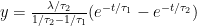
A linear combination of volcanic sulfates and CO2 changes were fit to the land-surface temperature history to produce Figure 5. As we will describe in a moment, the addition of a solar activity proxy did not significantly improve the fit. The large negative excursions are associated with volcanic sulfate emissions, with the four largest eruptions having all occurred pre-1850; thus our extension to the pre-1850 data proved useful for the observation of these events. To perform the fit, we adjusted the sulfate record by applying an exponential decay with a two year half-life following emission. The choice of two-years was motivated by maximizing the fit, and is considerably longer than the 4-8 month half-life observed for sulfate total mass in the atmosphere (but plausible for reflectivity which depends on area not volume).
OK, that makes me nervous … they have used a linear regression fit to the temperature record of the lagged exponential decay, with a separately fitted time constant, of an estimate of volcanic sulfate emissions based on ice cores … OK, I’ll buy that, but at a discount. They are using the emissions from here, but although I can get close to the figure above, I cannot replicate it exactly.
I wanted to extract the volcanic data. My plan of attack was as follows. First, I would digitize the heavy black line from Figure 1 above. Then I’d match it up with the logarithm of the CO increase since 1750. Once I subtracted out the CO2 increase, the remainder would be the hindcast change in temperature resulting from the volcanic eruptions alone.
Figure 2 shows the first part of the calculation, the digitized black line from Figure 1 (CO2 + volcanoes) with the log CO2 overlaid on it in red.
 Figure 2. The black line is the digitized black line from Figure 1. The red line is three times the log (base 2) of the change in CO2 plus an offset. CO2 data is from Law Dome ice cores 1750-1950, and from Mauna Loa thereafter.
I fit the CO2 curve to the data by hand and by eye, by manually adjusting the slope and the intercept of the regression, because standard regression methods don’t fit it to the top of the black line. A couple of things indicated to me that I was on the right track. First is the good fit of the log of the CO2 data to the BEST data. The second is that it turned out that the best fit is when using the standard climate sensitivity of 3°C for a doubling of CO2. Encouraged, I pressed on.
Subtracting the volcanic data from the CO2 data gives us the temperature change expected from volcanoes, as shown in Figure 3.
 Figure 3. Volcanic temperature changes (cooling after eruptions) as hindcast by BEST (black line), and as fit from the lagged emissions as described in their citation above (red line).
Note that as I mentioned above, I can get close to the temperature changes they hindcast (black line) using a lagged version of their sulfate data as they described (red line), but the match is not exact. Since the black line is what they show in Figure 1 above, and the differences are minor, I’ll continue to use the heavy black line.
Now, let’s pause here for a moment and consider what they have done, and what they have not done. What they have done is converted changes in atmospheric CO2 forcing in watts per square metre (W/m2) to a hindcast temperature change (in degrees C). They did this conversion by using the standard climate sensitivity of 3°C of warming for each doubling of CO2 (doubling gives an additional 3.7 W/m2).
They have also converted stratospheric injections of volcanic sulfates (in Teragrams) to a hindcast temperature change (in degrees C). They have done this by brute force, using a lagged model of the results of the stratospheric sulfate injections which is fit to the temperature.
But what they haven’t done, as far as I could find, is to calculate the forcing due to the volcanic eruptions (in W/m2). They just fitted the sulfate data directly to the temperature data and skipped the intermediate step. Without knowing the forcing due to the eruptions, I couldn’t estimate what climate sensitivity they had used to calculate the temperature response to the volcanic eruptions.
However, there’s more than one way to skin a cat. The NASA GISS folks have an estimate of the volcanic forcing (in W/m2, column headed “StratAer” for stratospheric aerosols from volcanoes). So to investigate BEST’s climate sensitivity, I used the GISS volcanic forcings. They only cover the period 1880—2000, but I could still use them to estimate the climate sensitivity that BEST had used for the volcanic forcings. And that’s where I found the curious part. Figure 4 shows the volcanic forcing in W/m2 from NASA GISS, along with the BEST hindcast temperature response from that forcing.
 Figure 4. Black line shows the BEST hindcast temperature anomaly (cooling) from the eruptions. Red line is the change in forcing, in watts per square metre (W/m2), from the eruptions. Green line shows the best fit theoretical cooling resulting from the GISS forcing. Note the different time period from the preceding figures.
As you can see, the regression (green line) of the GISS forcing gives a reasonable approximation of the BEST temperature anomaly, so again we’re on the right track. The curious part is the relative sizes. The change in temperature is just under a tenth of the change in forcing (0.08°C per W/m2).
This equates to a climate sensitivity of about 0.3°C per doubling of CO2 (0.08°C/W/m2 times 3.7 W/m2/doubling = 0.3°C/doubling)… which is a tenth of the canonical figure of three degrees per doubling of CO2.
So in their graph, in the heavy black line they have combined a climate sensitivity of 3°C per doubling for the CO2 portion, with a climate sensitivity of only 0.3°C per doubling for the volcanic portion …
Now this is indeed an odd result. There are several possible ways to explain this finding of a climate sensitivity of 0.3°C per doubling. Here are the possibilities
1. The NASA GISS folks have overestimated the forcing due to volcanoes by a factor of ten, a full order of magnitude. Possible, but very doubtful. The reduction in clear-sky sunlight following volcanic eruptions has been studied at length. We have a pretty good idea of the loss in incoming energy. We might be wrong by a factor of two, but not by a factor of ten.
2. The BEST temperature data underestimates the variation in temperature following volcanic eruptions by a full order of magnitude. Even more doubtful. The BEST temperature data is not perfect, but it is arguably the best we got.
3. The BEST data and the NASA data are both wrong, but providentially they are each wrong in the right direction to cancel each other out and give a sensitivity of three degrees per doubling. Odds are thin on that happening by chance, plus the reasons above still apply.
4. Both the NASA and BEST data are roughly correct, and the climate sensitivity actually is on the order of a tenth of what is claimed.
Me, I go for door number four, small climate sensitivity. I say the climate is buffered by a variety of homeostatic mechanisms that tend to minimize the temperature effects of changes in the forcing, as I have discussed at length in a variety of posts.
However, as always, alternative hypotheses are welcome.
Regards to everyone,
w.
DATA: I did this on an excel spreadsheet, which is here. While it is not user-friendly, I don’t think it is actively user-aggressive … the BEST temperature data on that spreadsheet is from here. Note that curiously, the BEST folks have not removed all of the annual cycle from their temperature data, there remains about a full degree of annual swing … go figure.
[UPDATE] Richard Telford in the comments points out that what I have calculated is the instantaneous sensitivity, and he is correct.
However, as I showed in “Time Lags in the Climate System“, in a system that is driven cyclically and that picks up and loses heat via exponential gain and decay, the instantaneous sensitivity is related to the longer-term sensitivity by the relationship

where t1 is the lag, t is the length of the cycle, and s2/s1 is the size of the reduction in amplitude. Since in this case we are dealing with the BEST land-only temperatures, where the lag is short (less than a month on average) that means that the short-term sensitivity is about 64% of the longer-term sensitivity. This would make the longer-term sensitivity about 0.46°C per doubling of CO2. This is still far, far below the usual estimate of 3°C per doubling.
Not concluded reading the post yet Willis but looking forward to it as i do with many of your posts. The early thing that struck me was Mosher not forthcoming with information? That seems odd given his proclivity for hounding others for data.
( as usual my full name available privately if required by anyone, I prefer a nickname, it’s been with me a looong time.)
“This equates to a climate sensitivity of about 0.3°C per doubling of CO2 (0.8°C/W/m2 times 3.7 W/m2/doubling = 0.3°C/doubling)… which is a tenth of the canonical figure of three degrees per doubling of CO2.”
Isn’t 0.8 x 3.7 almost exactly 3.0, rather than 0.3?
[My bad, should be 0.08, fixed. -w.]
Excellent post Willis. Makes more sense compared to the faffling Mosh and Co have done.
Letenus me throw another wrinkle, the cleaning of the atmosphere. Eruption introduces the dust, cosmic rays, or whatever create a moisture path, which moves with the wind, collecting the upper atmosphere dust, precipitating to the ground, reinforcing the hydraulic cycle, which is why a cold planet like mars, a hot planet like venus do not have many clouds like ours or too many clouds traping the heat into a runaway situation.
AFAIK climate sensitivity studies using observational evidence, not relying on climate models or paleoclimatic reconstructions, all show climate sensitivity to be low i.e. below 1C – 1.5C per doubling. All studies using climate models and paleoclimatic reconstructions show high climate sensitivity.
And isn’t climate sensitivity what this whole argument boils (oops) down to?
Makes me wonder why the IPCC prefer models and paleoclimatic reconstructions.
Willis you write “I’ve argued in a variety of posts that the usual canonical estimate of climate sensitivity, which is 3°C of warming for a doubling of CO2, is an order of magnitude too large.”
Could I suggest this ought to read “I’ve argued in a variety of posts that the usual canonical estimate of climate sensitivity, which is 3°C of warming for a doubling of CO2, is AT LEAST an order of magnitude too large.`
My capitals.
common sense – (technobabbel/1) = common sense
The conclusions as to forcings depends on belief in the GHG theory which is questionable at the best of times. Temperature accuracy is also questionable and not the best metric of climate because water content of the atmosphere at the point of measurement is ignored but vital is calculating heat available which is the real driver of weather/climate. But heat content has no relationship to atmospheric CO2 content but to solar insolation at the time.
Volcanic eruptions are more a proxy than a cause of any significant climatic changes beyond a year or two.
http://www.vukcevic.talktalk.net/Ap-VI.htm
Ignore or take a note makes no difference to the climate, but it might help to the understanding.
Possibility 5. Eschenbach’s methods are unfit for purpose (not for the first time).
Volcanic forcings are of short duration so the climate system, especially the oceans, does not reach equilibrium. Therefore, dividing the temperature change by the forcing is guaranteed to underestimate sensitivity.
Willis,
Firstly, I think you mean ‘0.08’ rather than ‘0.8°C per W/m2’.
Secondly, you’re missing the different timescales involved in CO2 versus volcanic forcing. Volcanic forcing is near-instantaneous, and is followed up a couple of years later with a quick forcing increase as aerosols are scrubbed. Conversely, CO2 has been accumulating gradually, with a persistent forcing in the same direction over the ~200 year period.
The best comparison to use for applying some form of check on your hypothesis are model outputs from 2xCO2 instantaneous forcing scenarios. There’s one in Climate Explorer for the GISS-EH model. I’ve produced output files for the land and land+ocean data (I don’t know how long these files stay on their servers, but you can output new ones yourself). If you look at these files, 10 years after a ~4W/m^2 forcing there is about 0.5ºC temperature increase (land, ~0.25ºC land+ocean) despite the fact that its ECS is 2.7ºC.
Willis-
There is a typo here- “The change in temperature is just under a tenth of the change in forcing (0.8°C per W/m2).”
Should be 0.08 C per W/m^2, no?
The same typo also appears here- “This equates to a climate sensitivity of about 0.3°C per doubling of CO2 (0.8°C/W/m2 times 3.7 W/m2/doubling = 0.3°C/doubling)…”
Should be 0.08C/W/m2.
Also, the GISS forcing of just under 3 W/m^2 at peak for Pinatubo is anomalously small when compared with the measured change in optical opacity of the atmosphere which peaked at 0.15 in the visible, giving a negative forcing of about 35 W/m^2 at peak, or ten times larger than what GISS climate models expectorate.
Last time I checked, 0.8×3.7 was 2.96.
Two little questions for you. First, how long do volcanic aerosols persist in the atmosphere, typically? And second, how long, all else being equal, would the atmosphere take to reach an equilibrium response to the aerosol forcing?
Oh, and one more if you would – roughly how many scientific papers which make estimates of the climate sensitivity have you read?
Willis: In your past posts about volcanoes, have you looked at the response of Land+Sea Surface Temperature data, like GISS LOTI, to the Mount Pinatubo eruption? If so, what was the maximum initial temperature drop that you found for it?
hmmm, don’t worry Willis, Mosher will be along real soon with a cryptic clue as to where you went wrong. I am sure his cryptic clues will be enough to satisfy everyone that BEST are doing their best.
Personally I think you are doing better than BEST.
Well, you can hit someone with the same strength, but depending where, how and with what you hit him, the pain can be quite different….
This simplistic comparison between the temperature response to a doubling of co2 or a volcanic eruption just doesn’t make a lot of sense.
The “canonical” estimate does not come from the Vatican, sole source of authorized canon, after lengthy conciles!
Let’s see how your finding correlates with model calculation.
So far models go like this:
– for any doubling of CO2 the forcing will be ΔF = 5.35 · ln(C/Co) = 5.35 · ln(2) = 3.7 W m-2. This is a physical spectrometric finding, not related to climate. Not too much to be discussed here.
– responding to such a forcing, and looking for a equilibrated energy balance, the primary temperature increase shoud be approx. 0.8°C. Other global models may offer little differences (before any feedback consideration). Regional variations may be larger in some places (e.g. Northern hemisphere) and smaller somewhere else.
– taking into account an overall negative feedback of -1.3 W m-2 K-1 from all known mechanisms (Planck, water vapour, lapse rate, albedo, and clouds. See: http://journals.ametsoc.org/doi/pdf/10.1175/JCLI3819.1) this temperature response is reduced by half to approx. 0.6°C.
Neo-Vatican: IPCC’s basic feedback assumption is that an overall negative feedback of -1.3 W m-2 K-1 will provoke a positive temperature increase of 3.7/1.3 = 2.85 °C. This is dimensionally OK, but an absolute physical non-sense: negative feedback provoking positive reinforcment, infinitely small feedback with infinitely high system response. This was never discussed nor criticized in any paper, but blessed by the IPCC report committee, presided by authors of this non-sense.
This means that any temperature increase that would surpass 0.6°C would probably be due to other [non anthropogenic] factors than doubling CO2 atmospheric concentration by human made emissions.
And please note that we are far from doubling: we are at approx. 395 ppm as compared to historical pre-industrial 280 ppm (if we accept this baseline), just a 41% increase. So we speak here of approx. 0.4°C temperature increase attributable to CO2 emissions since two centuries.
Willis: your findings, taken out of temperature records statistics, is 0.3°C for any doubling. This would mean that homeostatic mechanisms are stronger than assumed in the underlying feedback paper wher a wide uncertainty range is also given.
Anyway, it’s difficult to establish a therory based on experimental work since we have only one Earth and one experiment. Let’s remain in conjectures.
John Marshall says:
August 13, 2012 at 6:53 am
The conclusions as to forcings depends on belief in the GHG theory which is questionable at the best of times.
How much heat could atmospheric CO2 possibly impart on the oceans compared to other factors: For instance a hundred year increase in solar activity compared to total atmosphere density and composition changes?
What about local CO2 concentrations? In a closed system, where CO2 is suggested to have such a dynamic effect on temperature, then a greenhouse with 1200 ppm parked next to a greenhouse with 120 ppm should demonstrated a very significant temperature difference.
Willis, always enjoy your enlightening and easily followed posts. Anyone who has been trained in or exposed to process control theory knows that a system dominated by positive feedbacks will saturate at one extreme or the other until affected by a dominant outside forcing! Earth has experienced at least two periods or near total glacial encapsulazation – 600 m & 2.4 b years ago. However, there is no indication that the Earth has even been more than 7C warmer than today. The obvious conclusion is that Earth’s climate is dominated by negative feedback that are periodically and also sporadically overridden by external forcings. Melankovich cycles are an obvious such external forcing. Sun spot cycles plus Dalton, Maunder et al minima are more frequent perturbations to Earth’s climate. Contiental drift and location near the equator is another long cycle forcing.
CO2 concentrations are estimated to have reached 7,000 ppm (4 doublings from today’s 400 ppm) but we have no evidence of runaway warming. CO2 and GHG’s may have a small impact, but trivial at best. I, therefore, agree with your estimate of 0.3C/doubling at MOST!
I’m very disappointed that process control engineers and professors around the world have not raised their voices in protest of this absurd AGW movement!
Bill
The likely reason why the apparent sensitivity for the long term change is large is because it’s land temps, rather than global surface temps. The change is very likely larger.
BTW Willis, surely .8/W/m^2 should be .08, other wise the change is almost exactly 3 C per doubling-which is again, even if correct, not the right answer due to completely excluding the ocean. There is a lot that’s wrong with the BEST “attribution”-the linear regression approach completely ignores physics and gives inconsistent answers.
Echo chamber criticisms and affirmations aside, thanks for doing this. Paul S’s comment above is cogent – and I suspect if you followed it through, you’d get a number for sensitivity >0.3. However, I’ll guess it will also be a lot less than 3.0. Take odds?
“The choice of two-years was motivated by maximizing the fit, and is considerably longer than the 4-8 month half-life observed for sulfate total mass in the atmosphere”
This is all about forcing the data to fit the theory – the exact OPPOSITE of science, but the also the EXACT rationalization of theology.
In other words, “We know what we know and we will not be confused by the facts.”
Degree of “forcing” is indeed a critical factor in any self-dealing Warmist model. Alas, facts to hyper-politicized propagandists are immaterial. What might yet resolve this issue to mutually impartial, objective, rational satisfaction? Given the wholly qualitative nature of Warmists’ meretricious reliance on non-empirical data, we fear the answer is: Nothing.
“Me, I go for door number four, small climate sensitivity. I say the climate is buffered by a variety of homeostatic mechanisms that tend to minimize the temperature effects of changes in the forcing, as I have discussed at length in a variety of posts.”
Could you also present us the links of the “variety of posts” so we can verify them ourselves please?
richard telford says:
August 13, 2012 at 6:57 am
Gosh, telford, do you work at being snide, or is it just your natural state of being?

Number 5 is always a possibility … but in this case you haven’t thought the question all the way through. As I showed in “Time Lags in the Climate System“, in a system that is driven cyclically, the instantaneous sensitivity is related to the longer-term sensitivity by the relationship
where t1 is the lag, t is the length of the cycle, and s2/s1 is the size of the reduction in amplitude. Since in this case we are dealing with the BEST land-only temperatures, where the lag is short (less than a month on average) that means that the short-term sensitivity is about 64% of the final sensitivity. This would make the final sensitivity about 0.46°C per doubling of CO2.
w.
Michel says:
August 13, 2012 at 7:43 am
Merriam-Webster: canonical 2. conforming to a general rule or acceptable procedure : orthodox
w.
Michel says:
August 13, 2012 at 7:43 am
“The “canonical” estimate does not come from the Vatican, sole source of authorized canon, after lengthy conciles!”
Only pronouncements regarding Church dogma, such as the Trinity, are considered infallible as they are inspired by the Holy Spirit. When these are announced the Pope uses the term “WE” referring to himself and the Holy Spirit. Perhaps the IPCC is also conferring with the Holy Spirit prior to their pronouncements.
Robbie says:
August 13, 2012 at 10:08 am
Thanks, Robbie, be glad to. I finished writing the head post at 3:40 AM this morning, so I couldn’t be bothered hunting down the links at the time.
You might start with “The Thunderstorm Hypothesis“. Then take a look at “It’s Not About Feedback“, and “The Details Are In The Devil“. Follow that up with “Further Evidence for my Thunderstorm Thermostat Hypothesis“. For a chaser, try a look at yet another homeostatic mechanism in “Argo and the Ocean Temperature Maximum“.
That’s not an exhaustive list, I have more for when you finish those …
w.
Robbie, you asked for it. Enjoy your reading assignment, it should keep you busy for a few hours at least.☺
..speaking of Biblical faith driven belief.. Noah had a very competant weather forecaster. Maybe the CAGW crowd should look to some other faith for inspiriation. They obviously do not practice their current faith other than passing the plate.
Just a personal comment, but is there someway to do away with the endless spelling mistake and typographical comments.
If one wants to disrupt a comment blog these days, the simplest way is to point out small typos and then re-comment on the same typos that someone else commented on earlier. And just keep doing that over and over.
At RealClimate, each individual could get in maybe 10 comments like this on each thread.
John Daly used 6 different methods to calculate climate sensitivity.
The average warming predicted by the six methods for a doubling of CO2, is only +0.2 degC.
http://www.john-daly.com/miniwarm.htm
So your 0.3C for a doubling of CO2 is right in line with his estimates.
And I am sceptical of the effects of the Laki eruption. Laki was an effusive eruption and unlike Plinian eruptions didn’t inject sulphates into the stratosphere. Which says to me, either the standard explanation of volcanic cooling from stratospheric sulphate aerosols is wrong or BEST’s cooling from the Laki eruption is fictional.
http://www.agu.org/pubs/crossref/2012/2011GL050075.shtml
Outstanding work, BTW.
Michel says: “The “canonical” estimate does not come from the Vatican, sole source of authorized canon, after lengthy conciles!”
I believe it’s also mandatory to wear funny hats to issue canonical works. Here’s just one such bit of headgear:
http://i2.listal.com/image/892019/936full-jeremy-brett.jpg
Willis, a fantastic and excellent post showing once again, that observations show a much more insensitive climate system than what is depicted by models. The power of a forcing to make the temperature rise One Degree C is 12.5 w/m^2 in the sensitivity that you calculated, making this considerably higher value than Spencer and Lindzen’s estimates of Climate Sensitivity (around 5-7w/m^2 for a Degree C of warming, which would still represent large negative feedback). This would represent about a 0.13 Degree C anthropogenic contribution to the 20th Century Warming at equilibrium, assuming that the IPCC’s net radiative forcing for all Anthropogenic sources combined is right (about 1.6 w/m^2). This is not nearly enough to explain the warming over the 20th Century.
“climate is buffered by a variety of homeostatic mechanisms that tend to minimize the temperature effects of changes in the forcing”
Dude, that’s the long winded way of saying Gaia. Awesome, I knew it all along. Mother Nature lives! Attempting straightforward models of the climate is a fools errand.
I’ve overlayed the Dalton Minimum solar cycle TSI numbers (from Kopp and Lean 2011) onto the notorious 1775 to 1825 cold period.
Also shown is the exact date of the three major volcanoes and Berkeley Earth’s temperature numbers over the period.
There is a small effect from the volcanoes but looking at the high-resolution data makes it clear that the volcanic forcing attribution is way overblown. Temperatures went up after the 1809 unidentified eruption.
I would be tempted to conclude the solar cycle is responsible for the low temperatures in the period. There wasn’t much of solar cycle in terms of TSI changes in the Dalton Minimum.
http://s12.postimage.org/7mrm9mzf1/Berkeley_1775_to_1825.png
You might be dealing with land only temperatures, but I hope don’t imagine that land temperatures are independent of ocean temperatures. Any idea that the oceans have a lag of less than a month would be pretty crazy. Nevertheless, I have complete confidence that you will be able to conceive an analysis that will return an ocean lag this short.
The devil is in the pudding!
As been alluded to in a previous post ..how do know that all eruptions have injected suplhates in to the atmosphere.?
Thanks once again, Willis.
I wonder if the differences are in the feedbacks. Maybe they don’t consider the volcanoes contribution gives feedback with water vapour, whereas CO2 creates feedback from water vapour. Or is it the other way around.
Willis,
I’d be interested in your comments on John Daly’s methods, please ?
http://www.john-daly.com/miniwarm.htm
They seem very simplistic but support your conclusions.
Willis on your possibilities.
This looks like an important reference for the NASA volcano forcing
http://arxiv.org/ftp/arxiv/papers/1105/1105.1140.pdf
(see section 12.3. Stratospheric aerosol forcing page 25)
In that sect hansen writes
“The ability of radiation calculations to simulate the effect of stratospheric aerosols on
reflected solar and emitted thermal spectra was tested (Fig. 11 of Hansen et al., 2005) using
Earth’s measured radiation balance (Wong et al., 2005) following the 1991 Pinatubo eruption.
Good agreement was found with the observed temporal response of solar and thermal radiation,
but the observed net radiation change was about 25 percent smaller than calculated. Because of
uncertainties in measured radiation anomalies and aerosol properties, that difference is not large
enough to define any change to the stratospheric aerosol forcing. ”
So a four fold difference between observation and theory isn’t enough to cause a hiccup. You maybe a bit too generous when you write “We might be wrong by a factor of two, but not by a factor of ten.”
If the estimate of 0.46 degrees Celsius for a doubling of CO2 was combined with the assumption of 3.7 W/m^2 from that, then the result would be 0.12 K/W*m^2 climate sensitivity.
(Climate sensitivity then would be around 0.08 K/W*m^2 short-term and around 0.12 K/W*m^2 long-term).
Such could be about right. Dr. Idso estimated climate sensitivity by several different means in a paper; some appeared doubtful, but others seemed good. He got a figure which was similar (IIRC, 0.11 K/W*m^2 and 0.4 degrees Celsius for a CO2 doubling, although that is from memory and not double-checked).
It is less than Dr. Shaviv’s estimates, but, as much as I respect and applaud his work, his solar+GCR-based estimates have the weakness of being without attempting to take into account other factors such as ocean cycles at the same time as reconstructing temperature data without the CAGW movement’s fudging of it (with doing all at once being a difficult lengthy task which absolutely nobody has ever even seriously attempted as far as I’ve seen amongst many papers).
Such would mean the cosmic ray flux difference between the Little Ice Age and now ought to be really large, but that is conceivable enough, like Be-10 data illustrates ( http://www.freeimagehosting.net/newuploads/319xq.jpg ).
**********************
On the other hand, BEST is a fudged and false dataset overall, managed by an activist who briefly faked being a skeptic (with utter contradiction between figure 1 and the pre-fudging graphs illustrated in my August 9, 2012 2:26 pm and other comments in http://wattsupwiththat.com/2012/08/06/nasas-james-hansens-big-cherry-pick/#comments ). On yet the other hand, though, usually the standard procedure for fudging is spreading it out gradually over long periods of time, so such as relative figures from just one year to the next may be relatively close enough to accurate in themselves for the volcano analysis (with most year-to-year inaccuracy being far less than cumulative inaccuracy over decades).
If I understand it correctly, the BEST paper uses the data in a straight curve fitting exercise and doesn’t test the regression by using some of the data as a calibration period and then extrapolating to a training period for which we have historical data to compare against to see if their assumptions work. (they don’t).
This is an abysmal FAIL. It is not how SCIENCE is conducted.
Richard Telford
“Equilibrium”? What are you talking about? Equilibrium is practically never reached in the climate system – if it were then winds and ocean currents would cease, a nightmare scenario.
As a far-from-equilibrium system the climate displays nonlinear-nonequilibrium (quasi chaotic) dynamics, making simplistic linear estimates of sensitivity inappropriate. Please read Bill Yarber’s post on feedbacks from the control engineering perspective. The role and effects of feedbacks are quite different in a nonequilibrium nonlinear pattern system impacting primarily oscillation rather than sensitivity. The platinum-catalysed oxidation of CO is a classic experimental system to see this at work. An important characteristic of such systems is Lyapunov stability resulting in – as Willis concludes – limited and damped response to external forcings.
Watched the “day after tomorrow” yesterday on return from holiday. Realised that this would be the way future generations would see the climate hysteria of the naughties. In other words, they are going to believe we all thought … global warming was going to cause an ice-age.
Future generations are going to look at ours with the same incredulity of … “flat-earthers” (which is itself a false view of what people believed in the past) or of King Canute (who was trying to make a point that his advisers were wrong and humans couldn’t command nature … which is kind of apt),
We are going to look absolutely daft. Not only is global warming going to turn out to be almost completely false but the logic of the doomsday scenario will be that portrayed by holywood in the day after tomorrow, and not what any climate academic tried to say.
willis, the Berkeley graph shows 7 eruptions since 1750 with one Laki,
see one comment, did not reach the stratosphere…The next, the GISS
graph shows 10 volcano eruption spikes downward since 1880…….
Now, where are all those many other eruptions, in particularly those, in
which there is NO spike downward but with a temp spike upward? Eruptions
which occurred in the midst of a decade with temp increase?
There are a good many more major eruptions not mentioned…..JS
mycroft says:
August 13, 2012 at 1:07 pm
Each eruption is different, as different as the composition of the underlying geology, as different as the size and nature of the eruptions. Some inject sulfur into the stratosphere, where it is carried around the globe, and some don’t.
We know who is who by analyzing the ice cores for the presents of sulfates. When sulfur is injected into the stratosphere, it eventually falls out all over the planet, including near the poles where it is captured and preserved in the ice cores. The timing and amount of that sulfate deposition is then used to back-calculate the amount that was injected into the stratosphere.
This is all explained, at least to some degree, in the paper cited in the BEST study.
w.
chris y says:
August 13, 2012 at 7:11 am
Thanks, Chris. You need to consider the distribution of the particles, and to do that you need a global distribution of measurements … or faith in climate models, which for this simple analysis (diffusion from a point source) might be adequate. I suspect the difference between your figure and theirs relates to that.
w.
Jose says:
August 13, 2012 at 7:20 am
Depends among other things on the type and size of the aerosol, whether it is water-soluble, and whether it is injected into the stratosphere or not.
No exact answer can be given, since it will approach equilibrium gradually, and it never “arrives”.
It doesn’t take that long for land to respond to increased forcing. The thermal lag in the annual cycle (the time between the summer solstice and the warmest time of the year) is under a month for the earth’s land surface.
Finally, since the warming to equilibrium is exponential, we see the largest effect of the warming right away, and it then warms at a slower and slower rate into the future. This means that it gets near to equilibrium quickly.
I have 700 papers that mention the term here on my computer. I can’t say I’ve pored over them all, but I have scanned them all, read most of them, and pored over and revisited many of them.
And you? Roughly how many scientific papers which make estimates of the climate sensitivity have you read?
Here’s the thing, Jose. It doesn’t matter how many I’ve read. All that matters is whether my ideas are true and valid. That’s all that counts. And yes … in addition to having interesting and perhaps valid ideas, I have also done my homework.
All the best,
w.
Bob Tisdale says:
August 13, 2012 at 7:24 am
Willis: In your past posts about volcanoes, have you looked at the response of Land+Sea Surface Temperature data, like GISS LOTI, to the Mount Pinatubo eruption? If so, what was the maximum initial temperature drop that you found for it?
Thanks, Bob. See my posts “Prediction is hard, especially of the future“, and “Pinatubo and the Albedo Thermostat“.
w.
Some updated data showing Berkeley versus Total Solar Irradiance back to 1753.
Not a close link but I note that Berkeley’s algorithm probably overstates the real warming trend by about 35% (based on numerous comparisons with other known temperature datasets which indicates that Berkeley’s record splitting algorithm probably favors breakpoints that go down versus breakpoints that go up).
http://s10.postimage.org/f2qsk2nqx/Berkeley_TSI_1753.png
Mr. Eschenbach’s assertion that the climate sensitivity is “a tenth of the canonical figure of three degrees per doubling of CO2” runs a foul of the scientific illegitimacy of the contention that the climate system has a “climate sensitivity” as a property.
By definition, the “climate sensitivity” is the ratio of the change in the spatially averaged equilibrium surface air temperature to the change in the logarithm to the base 2 of the CO2 concentration. The equilibrium temperature is not an observable and it follows that when folks, including Mr. Eschenbach, speculate about the numerical value of the climate sensitivity, these speculations are insusceptible to being refuted by reference to measurements of the (unobservable) equilibrium surface air temperature.
willis the data is cited in the paper with a url as many people explained to you
ftp://ftp.ncdc.noaa.gov/pub/data/paleo/climate_forcing/volcanic_aerosols/gao2008ivi2/ivi2totalloading501-2000.txt
And the other dataset used per Gao’s instructions is here
http://data.giss.nasa.gov/modelforce/strataer/
“I have 700 papers that mention the term here on my computer.”
Willis, that argument appears to be the key one in this post-normal science. Academics no longer argue from the evidence, instead they argue from the count of papers as if it had any meaning at all in science.
In other words, it’s a lemming approach … all the other idiots believe the way forward is over the cliff so …. they too must be stupid and jump over the cliff.
Philip Bradley says:
“And I am sceptical of the effects of the Laki eruption. Laki was an effusive eruption and unlike Plinian eruptions didn’t inject sulphates into the stratosphere.”
The Laki eruption in 1783 is the only large scale fissure eruption that has occurred on Earth in historical times. That means that we have no data to compare it with so as to how effective such eruptions are in injecting materials into the stratosphere. However to call it “effusive” is perhaps a bit tame. Icelandic sources describe lava fountains reaching a height of a kilometer or more, and the extreme rate of lava discharge would have caused convection more than sufficient to carry part of the SO2 into the lower stratosphere (even thunderstorms can do that).
Contemporary sources makes it very clear that the eruption had extreme atmospheric effects both in the near and far field. I tend to believe those sources more than current speculation.
Terry Oldberg:
At August 13, 2012 at 8:34 pm you say
Please explain why you think the “equilibrium surface temperature” needs to be known – or is relevant – to refutation of an estimate or a speculation of climate sensitivity.
Richard
richardscourtney:
Thank you for giving me the opportunity to clarify. The climate sensitivity (aka equilibrium climate sensitivity) is the proportionality constant in an equation that maps the change in the atmospheric CO2 concentration to the change in the logarithm to the base 2 of the spatially averaged equilibrium surface air temperature. When it is asserted that the climate sensitivity has a particular numerical value (e.g. 3 Celsius per doubling of the CO2 concentration), this assertion is insusceptible to refutation because the equilibrium temperature (aka steady-state temperature) is not an observable feature of the real world.
As assertions of numerical values for the climate sensitivity are insusceptible to refutation, a science of climate change cannot be built around them. On the other hand, spatially averaged surface air temperatures are an observable feature of the real world and thus a science of climate change could be built around them. This science would have as components: 1) a theory 2) conditional predictions by this theory of the spatially averaged surface air temperatures in the events forming a specified statistical population and 3) validation of this theory in a sampling of events drawn from this population and observed. A consequence from methodological blunders on the part of professional climatologists is for none of these components to currently exist. After decades of work and the expenditure of more than 100 billion US$ on research, we have no science of climate change and this is true even though many professional climatologists insist that one exists.
Willis Eschenbach: “in a system that is driven cyclically, the instantaneous sensitivity is related to the longer-term sensitivity by . . . ”
Could you expand on how you apply to the problem at hand the equation you thereupon set forth? More specifically:
Willis Eschenbach: “Since in this case we are dealing with the BEST land-only temperatures, where the lag is short (less than a month on average) that means that the short-term sensitivity is about 64% of the final sensitivity.”
Could you explain how you plug “short (less than a month on average)” into that equation? The equation you’re applying deals with diffusion phenomena, and it relates the time lags between sinusoidal variations at different diffusion depths to those variations’ amplitudes (and the variations’ periods). My difficulty is identifying the cyclical signal. In infer from your “64%” that you observe a phase lag that is -0.159 log(0.64) = 7.1% of the cyclical signal’s period. It would be helpful if you could identify the cyclical signal, period, and lag you used. If you could be explicit about where you see an analog to diffusion depth, that, too, would be helpful.
Mosh, still doesn’t mean squat if the model isn’t tested. Calibration and training periods? Ever heard of them? I know you have, since you discussed them at length on Steve MacIntyre’s blog years ago.
Highflight56433 asks about atmospheric density and composition. Atmospheric density increase will result in an increase in temperature, as per the combined gas laws, regardless of composition. As to the greenhouse experiment with differing concentrations of CO2, I have not seen the results of any experiment along this track but would bet on no temperature difference assuming the same inputs. Anthony Watts experiment was similar, but the CO2 concentrations were not accurately known, but showed no temperature difference to a lower temperature in the vessel with the higher CO2 concentration. To my knowledge he has not repeated this with higher accuracy but time will tell.
Again, I don’t get the point of this article…the climate sensitivity is quite different whether the external forcing is a doubling of co2 or volcanic aerosols, so the comparison cannot be done like this…
JJ:
At August 14, 2012 at 2:29 am
the climate sensitivity is quite different whether the external forcing is a doubling of co2 or volcanic aerosols,
Richard
IS THE NON-FEEDBACK CLIMATE SENSITIVITY 1.2 OR 0.6 DEG C?
Using the Stefan-Boltzmann equation
Q = kT^4 (Equation 1)
Where Q is the radiation energy emitted by the surface of the earth and k = 5.67 x 10^(-8) W/(m^2 K^4)
Differentiating Equation 1 with respect to T gives:
dQ/dT = 4kT^3 = 4*(kT^4)/T = 4Q/T (Equation 2)
Taking the reciprocal of the above equation gives:
dT/dQ = T/(4Q) (Equation 3)
From the above equation, the small change in global mean temperature dT as a result of change in the emitted radiation energy dQ by the globe may be calculated using the equation:
dT = T*dQ/(4Q) (Equation 4)
At equilibrium condition, the radiation energy Q emitted by the earth is assumed to be equal to the solar energy absorbed at the earth’s surface:
Q = (1-a)Sp/2 (Equation 5)
In this equation, Sp is the solar constant of 1370 W/m^2 at the mean distance of the earth from the sun distributed on its projected area Ap = Pi*r^2. Instead of the projected area, the solar energy from the sun is actually distribute around half of the spherical surface area As = 2*Pi*r^2. As a result, the solar energy distributed around half of the spherical surface area is given by Ss = Sp* Pi*r^2/(2*Pi*r^2) = Sp/2. The solar energy Ss does not reach the surface of the earth because part of it given by a*Ss is reflected by the atmosphere, where “a” is the albedo of the atmosphere. Therefore, the solar energy that reaches the surface of the earth is Ss-a*Ss = (1-a)Ss = (1-a)Sp/2.
Equation 5 could also be written as:
4Q = 2*(1-a)Sp (Equation 6)
Substituting Equation 6 into 4 gives:
dT = T*dQ/(2*(1-a)*Sp) (Equation 7)
The increase in forcing for doubling of CO2 is estimated to be dQ = 4 W/m^2. The global mean temperature is T = 288 K, the earth’s albedo is a = 0.3 and the solar constant Sp = 1370 W/m^2. Substituting these values into Equation 7 gives an estimate for the non-feed back climate sensitivity:
dT = 288*4/(2*(1-0.3)*1370) = 288*4/(2*0.7*1370) = 0.6
This means that the non-feed back climate sensitivity of the earth is 0.6 deg C for doubling of CO2.
Do you agree?
JJ: the climate sensitivity is quite different whether the external forcing is a doubling of co2 or volcanic aerosols,
richardscourtney says:
Really?! Please explain why.
Come now Richard, isn’t it obvious? The noxious gases, particulates, etc. from volcanoes are natural and therefore good, whereas CO2-plant food is man-made and therefore bad.
Let’s not forget that there are volcanoes… and there are volcanoes… There are many different types of eruptions depending on the volcano’s geology. They’re all different. And then there are all of the undersea volcanoes – who knows how many there are of those? Volcanoes are erupting somewhere all the time.
Why does volcanic forcing in W/m2 have such a small impact compared to GHG forcing in the same W/m2.
Willis notes that the climate adjusts to offset some/most of the forcing. The climate models also had built in some of this dampening effect initially and then they lowered it even further through an “efficiency factor” when it was realized the impact was even less than dampened impact.
Okay, so volcanoes have less impact than one would initially assume given the reduction in solar energy reaching the Earth’s surface in W/m2. The climate models have been downscaled to simulate the actual impact versus the theoritical impact. Berkeley changed it to 1.5C per Tg of Sulfate emission (and this is still too high given the sulfate dataset they used is poor and they did compare it to the high resolution temperature data but rather eye-balled it, it seems).
So, what faith do we then place in the temperature impact per W/m2 of GHG forcing. Why are we still stuck at 0.8C/W/m2 when it is starting to look every day like this is off by a factor of at least 2 (just like the volcanic forcing was off by a factor of 7 to 10).
Willis:
I don’t think you have showed anything new here from what you did with the seasonal cycle stuff you were looking at. What you are showing is that if you assume the climate system is well-modeled as having a single time constant and that said time constant is short then you indeed get very low estimates for the climate sensitivity.
However, you haven’t provided any evidence that the climate system is in fact well-modeled by having a single time constant and that said time constant is short and, in fact, this contradicts a lot of what is currently understood about the climate system.
Girma says:
You have two major errors here:
(1) The average intensity of solar radiation to use is not Sp/2; it is Sp/4. This is because the sun intercepts an amount of power equal to Sp*(Pi*r^2) but radiates at the rate given by the Stefan-Boltzmann Equation over the entire 4*Pi*r^2 area of its surface. There is a factor of 4 difference between Pi*r^2 and 4*pi*r^2.
(2) The correct temperature to use for the Earth is the effective radiating temperature of 255 K.
If you correct these two errors, you get about 1.06 C, which is basically the accepted value. (There is a slight correction for the fact that the warming is non-uniform, which raises the best estimate of the no-feedback sensitivity to about 1.2 C.)
Steven Mosher says:
August 13, 2012 at 8:48 pm
Steven Mosher says:
August 13, 2012 at 8:53 pm (Edit)
I cited and talked about both of those datasets above in the head post and in the comments. Do try to keep up with the discussion.
w.
Joe Born says:
August 14, 2012 at 1:42 am
Thanks as always for your questions, Joe. We have a system where the earth both absorbs and loses energy on a cyclical basis. The result of this is that the peak temperature lags the peak insolation. In such a system, the longer the lag, the less the system heats up or cools down. This makes intuitive sense, as something that warms and cools faster will get hotter (and colder) when driven cyclically than something that warms and cools more slowly.
As you point out, volcanoes are not a cyclical phenomenon … but they are an approximately half-wave driving cycle, so we can use the same relationship. The question then becomes, how long is the cycle? I have made the most conservative estimate, that the cycle is a year and the half-cycle is six months, based on the observations of volcanic dust. As the BEST folks say, they discuss the “4-8 month half-life observed for sulfate total mass in the atmosphere”, so six months for the half-cycle is a reasonable estimate.
So what I have done is an estimate based on the known response time of the land to an approximately one-year cycle. I’ve done those calculations on a 1°x1° gridcell basis for a paper that I’m writing up for the journals. Although there are variations, the land of the planet has about a 0.8 – 0.9 month lag time with respect to the driving solar forcing, with the peak at 0.86.
As you have pointed out, this is all in the nature of an estimate … but that’s all we have. For example, the BEST forcing is an estimate as well, where they use a 2-year half-life for the stratospheric particles. Since my final climate sensitivity would be less if I assumed a two-year effective cycle for the volcanic forcing, I have made the conservative choice of one year.
All the best,
w.
Terry Oldberg:
Sincere thanks for your answer to my request for clarification which you provide at August 14, 2012 at 8:42 am.
Firstly, I say that I strongly agree with you when you say
Indeed, I go further in that I say a science of climate change will not be evinced until climate science stops the pseudoscientific search for confirmation of AGW and returns to scientific study of climate mechanisms.
That said, I return to the subject of climate sensitivity.
It is quite possible that the hypothesis of radiative forcing driving climate change(s) is plain wrong: I have explained this repeatedly including on WUWT. However, in the context of this thread, that radiative forcing hypothesis is taken as a given. Therefore, I am assuming it is true for the purpose of this discussion.
An observation of a change of known magnitude to radiative forcing can be compared to subsequent change to global temperature. This shows the ‘climate sensitivity’ of the cause of the change to radiative forcing. Indeed, Willis explains how he did this in the estimate he reports in his above article. He says:
etc.
The estimate will a variety of sources of error (any estimate of anything does). In this case, a major potential source of error is the time period chosen for completion of the effect of the change to radiative forcing. In reality the effect will never complete because it will continue to reduce at decaying rate of reduction towards equilibrium. And circumstances will change with time (to create a different equilibrium) so the effect will not achieve true equilibrium.
However, when the effect has reduced to a sufficiently small value (relative to errors in the estimate) then the effect can be assumed to have completed for practical purposes. Hence, the need to choose an appropriate time period for assumed effective completion (Willis says – and explains why – he chose a period of 6 months in his analysis).
The important point is that the true equilibrium is not relevant: only selection of the appropriate time period for effective equilibrium is need. There is a caveat to this in that more than one equilibrium condition may exist (e.g. an equilibrium over land and a different equilibrium over oceans). Indeed, in this thread Joel Shore has asserted that two time constants are needed because of this caveat. However, this is not true if an appropriate time period for all the equilibria is used.
So, when you said at August 13, 2012 at 8:34 pm
I asked August 14, 2012 at 1:16 am
I am grateful for your reply to that question at August 14, 2012 at 8:42 am and which I am now answering. However, it does not resolve my failure to understand your point.
Your reply says
As I have said, I agree we need a science of climate change, but I fail to see how that is relevant to your point which I queried.
In this response I have tried to explain why I have difficulty understanding why knowing climate equilibrium state is relevant to the validity of climate sensitivity issues. And I regret that your answer to my question has not reduced my difficulty.
Richard
richardscourtney:
Ambiguity of reference by the term “climate sensitivity” (CS) to the associated ideas may be muddying the waters. I’ve used the term in reference to the change in the global equilibrium temperature from a specified change in the logarithm to the base 2 of the CO2 concentration (e.g., 3 Celsius per CO2 doubling). My conclusion of an insusceptibility to refutation seems to me to follow from this definition of the CS, for the magnitude of the CS is a function of the equilibrium temperature and this quantity is not observable. Do we agree on this?
‘Not concluded reading the post yet Willis but looking forward to it as i do with many of your posts. The early thing that struck me was Mosher not forthcoming with information? That seems odd given his proclivity for hounding others for data.
( as usual my full name available privately if required by anyone, I prefer a nickname, it’s been with me a looong time.)”
That would be for a couple reasons.
1. The core data is clearly linked to in the paper with the URL. read the footnotes.
2. we had to supplement that data with data from Sato as we discussed previously on Lucia’s
so I am bring it up at todays meeting to see if I can get a consolidated final file for folks.
I volunteer one day a week, so today is my day to go make my requests.
3. We are in the process of bringing up a public SVN so folks can get access that way since the code will have dependencies that can only be resolved if you have access to everything. That takes time and testing. 95% of the code is available via ftp, some of the code for doing figures may wait until actual publication as we are actively responding to reviewers. At the end branches would get gathered into the trunk. So today a branch may have tons of code and figures that never get published. Creating a package that has code to support all the published work in its final form while protecting work in progress ( like studies on heat waves, the SST work, work on satellites, diurnal trend work ) isnt an overnite gig.
phlogiston says:
August 13, 2012 at 4:35 pm
Richard Telford
“Equilibrium”? What are you talking about? Equilibrium is practically never reached in the climate system – if it were then winds and ocean currents would cease, a nightmare scenario.
——————————-
You are completely correct that the climate system never reaches equilibrium – the deep ocean and other slowly responding elements of the system do not have time to adjust before the climate forcing have changed. But your concept of what an equilibrium climate would look like is completely wrong. An climate that is in equilibrium still has weather, currents and waves, but there is no trend in the type of weather, strength of currents or size of waves. So, on average, the distribution of weather, currents and waves in each 30 year period would resemble that in all other 30 year periods under an equilibrium climate.
Just because the climate never reaches equilibrium does not mean that equilibrium climates are not a useful concept in the same way that an asymptote is a useful concept. Eschenbach is attempting to calculate a value for a concept known as equilibrium climate sensitivity, the amount of warming expected at equilibrium from a doubling of CO2. This cannot be done without reference to equilibrium climates.
tty says:
August 14, 2012 at 12:22 am
I agree there is a great deal we don’t know about the Laki eruption. One thing of note is that the peak of the Laki eruption, July 1783, was the hottest month ever recorded in the Central England Temperature record. Which is somewhat problematic for the volcanic cooling thesis.
http://cadair.aber.ac.uk/dspace/bitstream/handle/2160/230/Laki?sequence=3
Willis Eschenbach: “As you point out, volcanoes are not a cyclical phenomenon … but they are an approximately half-wave driving cycle, so we can use the same relationship.”

 ,
, .
.
 ,
,
I appreciate your taking the time to convey your reasoning. Despite that valiant effort, however, I haven’t yet gotten my mind around how you are able to treat the volcanic eruption as though it were cyclical. So I looked at the issue the way a layman (such as yours truly) would:
Suppose we have a stimulus of the form
applied to a system whose response to a unit step is:
i.e., to a system whose equilibrium output in response to a unity-step input is
We know that such a system’s response to the exponentially decaying input is given by
which tells us that for a stimulus that falls to half its initial value in two years (and thus has a time constant of 2.9 years), as Muller surmises, the system’s response reaches 89% of its unit-step equilibrium value if the system’s response to a one-year-period sinusoid has a 0.86-month lag (and therefore a time constant of 0.077 year), as you’ve found to be typical of land locations. If the system’s time constant is ten years, on the other hand–a proposition for which I’ve seen no compelling evidence—the response to that exponentially decaying stimulus would reach only 17% of its equilibrium value.
In short, my naive approach tends to support your view if your assumption about the speed of the earth’s response is correct.
The foregoing analysis obviously assumes a single-pole, lumped-parameter system, not the distributed-parameter system on which your equation is based. I have allowed myself to believe that the code accompanying my post at http://wattsupwiththat.com/2012/07/13/of-simple-models-seasonal-lags-and-tautochrones/ can be used to determine such a system’s response, but I haven’t taken the time to go through that exercise.
Terry Oldberg:
re your question to me at August 14, 2012 at 3:11 pm.
Yes, we do agree on that.
Richard
Willis:
“Here’s the thing, Jose. It doesn’t matter how many I’ve read. All that matters is whether my ideas are true and valid. That’s all that counts. And yes … in addition to having interesting and perhaps valid ideas, I have also done my homework.”
It does matter. If you had really read so many papers about climate sensitivity you might understand the simple flaws in your thinking that render your ideas invalid. I don’t think you really understand the time evolution of the forcing when you have an injection of aerosols into the upper atmosphere. Trying to estimate a climate sensitivity in the way you are doing cannot fail to give an incorrect answer, and if you were truly familiar with the literature you’d know that a more sophisticated approach is required.
Can I make the point that I’m sure other lurkers too are enjoying, from a purely spectator pov, with popcorn in hand, Willis & Mosher having a Celebrity Death Match, to see who can outsarc the other the most.
Very enjoyable.
The final data has been posted. In addition to the data linked to in the paper which Willis apparently missed ( see line 515 ) there is one line of that data that needs a correction.
The correction is described in the paper reference and must be added by hand. For people
who did not read the referenced papers and add the fix described in that paper, we supply
a full dataset along with some other information
Tallbloke for out of sample testing you can see these comments
http://rankexploits.com/musings/2012/on-volcanoes-and-their-climate-response/#comment-101529
richardscourtney:
Further to our conversation, Mr. Eschenbach’s “canonical” value of 3°C of warming for a doubling of CO2 is with the CS defined as I have stated it. It follows from the lack of observability of the global equilibrium temperature that this canonical value is insusceptible to refutation. Similar reasoning yields the conclusion that all non-canonical values for the CS are insusceptible to refutation. The lack of empirical refutability when a numerical value is asserted for the CS leaves the CS a scientifically useless concept. For scientific purposes, the CS does not exist, yet it plays a leading role in the IPCC’s argument for a significant level of global warming from the burning of fossil fuels.
Currently, studies of climate change do not rest on a scientific footing. In placing these studies on this kind of footing, climatologists would have to replace the unobservable global equilibrium temperature by an observable feature of the real world. One possibility is to replace it by the global average temperature over specified, non-overlapping time periods, e.g., periods of 3 decades each. To take this step would be to make a start on the task of defining the statistical population underlying the studies of the future. A statistical population is the sine qua non of a scientific study, for it supplies the necessary ingredient of refutability. Currently, we have no population.
All agreed, you are right in all….. but Willis proposes a micro-0.3 C CS
and how right/wrong is this micro-value? I bet he wants to know….
For a newcomer to climate science, the most informative comments thread I’ve seen on WUWT.
Mike, you can see, that volcanoes contribute nothing but a short
time dip of temps….we talk about a 5 years dip…? Or less? Of all
climate drivers, the smallest, the micro or nanodriver……does not
qualify to explain long term/presnt climate….
Willis is good, he has the hang of it on volcanoes, see his previous
volcano posts…..JS
Go over to Roy Spencers monthly global temp graph. He put:
“Pinatubo cooling” but not “El Chichon cooling”…. Why?
I complained various times that the “Cooling” should be taken out and
the 2010 El Nino “Warming” should be taken in….but “silencio…”….
The volcano-microdriver is obvious….big fuss about a little dip….
Steven Mosher says:
August 15, 2012 at 10:58 am
Thanks, Steven. To review the bidding, you had said:
And you gave a url that leads to a 401 not found.
I replied:
Now you’ve made the same claim a second time. I said it before. I’ll say it again. I referred to that data directly in the head post. You were wrong when you claimed above that I had missed it. You are wrong now when you claim it again. In the head post I said:
Note that when you click on that link, you get the data referred to in line 515 of the paper, the data you have twice accused me of missing or ignoring, the data that I both linked to and discussed in the head post..
w.
Joe Born says:
August 14, 2012 at 8:15 pm
Thanks as always for your analysis. The part that people miss when they say that the earth has a long time constant is that we only ever experience the surface of the land. A couple of kilometres (1.2 miles) beneath our feet, it’s 30 to 150°C hotter (54 to 327°F). The fact that it’s fiery hot a couple of kilometres down is meaningless. All that counts is the surface temperature.
And the land surface temperature changes quite quickly. If there is a one-time step increase in the energy absorbed by the surface, it will make a wave that propagates downwards through the ground. But the most of the change in the surface temperature occurs quite quickly … and the surface change is all that we experience, we are oblivious to the boiling hot temperatures a couple kilometers underneath us.
w.