Part II: How the central estimate of pre-feedback warming was exaggerated
By Christopher Monckton of Brenchley
In this series I am exploring the cumulative errors, large and small, through which the climatological establishment has succeeded in greatly exaggerating climate sensitivity. Since the series concerns itself chiefly with equilibrium sensitivity, time-dependencies, including those arising from non-linear feedbacks, are irrelevant.
In Part I, I described a small error by which the climate establishment determines the official central estimate of equilibrium climate sensitivity as the inter-model mean equilibrium sensitivity rather than determining that central estimate directly from the inter-model mean value of the temperature feedback factor f. For it is the interval of values for f that dictates the interval of final or equilibrium climate sensitivity and accounts for its hitherto poorly-constrained breadth [1.5, 4.5] K. Any credible probability-density function for final sensitivity must, therefore, center on the inter-model mean value of f, and not on the inter-model mean value of ΔT, skewed as it is by the rectangular-hyperbolic (and hence non-linear) form of the official system gain equation G = (1 – f)–1.
I showed that the effect of that first error was to overstate the key central estimates of final sensitivity by between 12.5% and 34%.
Part II, which will necessarily be lengthy and full of equations, will examine another apparently small but actually significant error that leads to an exaggeration of reference or pre-feedback climate sensitivity ΔT0 and hence of final sensitivity ΔT.
For convenience, the official equation (1) of climate sensitivity as it now stands is here repeated. There is much wrong with this equation, but, like it or not, it is what the climate establishment uses. In Part I, it was calibrated closely and successfully against the outputs of both the CMIP3 and CMIP5 model ensembles.
(1) ![]()
where ![]()
Fig. 1 illuminates the interrelation between the various terms in (1). In the current understanding, the reference or pre-feedback sensitivity ΔT0 is simply the product of the official value of radiative forcing ΔF0 = 3.708 W m–2 and the official value of the reference sensitivity parameter λ0 = 3.2–1 K W–1 m2, so that ΔT0 = 1.159 K (see e.g. AR4, p. 631 fn.).
However, as George White, an electronics engineer, has pointed out (pers. comm., 2016), in using a fixed value for the crucial reference sensitivity parameter λ0 the climate establishment are erroneously treating the fourth-power Stefan-Boltzmann equation as though it were linear, when of course it is exponential.
This mistreatment in itself leads to a small exaggeration, as I shall now show, but it is indicative of a deeper and more influential error. For George White’s query has led me to re-examine how, in official climatology, λ0 came to have the value at or near 0.312 K W–1 m2 that all current models use.

Fig. 1 Illumination of the official climate-sensitivity equation (1)
The fundamental equation (2) of radiative transfer relates flux density Fn in Watts per square meter to the corresponding temperature Tn in Kelvin at some surface n of a planetary body (and usually at the emission surface n = 0):
(2) ![]() | Stefan-Boltzmann equation
| Stefan-Boltzmann equation
where the Stefan-Boltzmann constant σ is equal to 5.6704 x 10⁻⁸ W m–2 K–4, and the emissivity εn of the relevant surface n is, by Kirchhoff’s radiation law, equal to its absorptivity. At the Earth’s reference or emission surface n = 0, a mean 5.3 km above ground level, emissivity ε0, particularly with respect to the near-infrared long-wave radiation with which we are concerned, is vanishingly different from unity.
The Earth’s mean emission flux density F0 is given by (3),
(3)  238.175 W m–2,
where S0 = 1361 W m–2 is total solar irradiance (SORCE/TIM, 2016); α = 0.3 is the Earth’s mean albedo, and 4 is the ratio of the surface area of the rotating near-spherical Earth to that of the disk that the planet presents to incoming solar radiation. Rearranging (2) as (4) and setting n = 0 gives the Earth’s mean emission temperature T0:
(4)  254.578 K.
A similar calculation may be performed at the Earth’s hard-deck surface S. We know that global mean surface temperature TS is 288 K, and measured emissivity εS ≈ 0.96. Accordingly, (3) gives FS as 374.503 W m–2. This value is often given as 390 W m–2, for εS is frequently taken as unity, since little error arises from that assumption.
The first derivative λ0 of the Stefan-Boltzmann equation relating the emission temperature T0 to emission flux density F0 before any radiative perturbation is given by (5):
(5) 
![]() 0.267 K W–1 m2.
0.267 K W–1 m2.
The surface equivalent λS = TS / (4FS) = 0.192 K W–1 m2 (or 0.185 if εS is taken as unity).
The official radiative forcing in response to a doubling of atmospheric CO2 concentration is given by the approximately logarithmic relation (6) (Myhre et al., 1998; AR3, ch. 6.1). We shall see later in this series that this value is an exaggeration, but let us use it for now.
(6) ![]() 3.708 W m–2.
3.708 W m–2.
Then the direct or reference warming in response to a CO2 doubling is given by
(7) ![]() 0.991 K.
0.991 K.
A similar result may be obtained thus: where Fμ = F0 + ΔF0 = 238.175 + 3.708 = 241.883 W m–2, using (2) gives Tμ:
(8)  255.563 K.
Then –
(9) ![]() 0.985 K,
0.985 K,
a little less than the result in (7), the small difference being caused by the fact that λ0 cannot have a fixed value, because, as George White rightly points out, it is the first derivative of a fourth-power relation and hence represents the slope of the curve of the Stefan-Boltzmann equation at some particular value for radiative flux and corresponding value for temperature.
Thus, the value of λ0, and hence that of climate sensitivity, must decline by little and little as the temperature increases, as the slightly non-linear curve in Fig. 2 shows.

Fig. 2 The first derivative λ0 = T0 / (4F0) of the Stefan-Boltzmann equation, which is the slope of a line tangent to the red curve above, declines by little and little as T0, F0 increase.
The value of λ0 may also be deduced from eq. (3) [here (10)] of Hansen (1984), who says [with notation altered to conform to the present work]:
“… for changes of solar irradiance,
(10) ![]() …
…
“Thus, if S0 increases by a small percentage δ, T0 increases by δ/4. For example, a 2% change in solar irradiance would change T0 by about 0.5%, or 1.2-1.3 K.”
Hansen’s 1984 paper equated the radiative forcing ΔF0 from a doubled CO2 concentration with a 2% increase ΔF0 = 4.764 W m–2 in emission flux density, which is where the value 1.2-1.3 K for ΔT0 = ΔF0λ0 seems first to have arisen. However, if today’s substantially smaller official value ΔF0 = 3.708 W m–2 (Myhre et al., 1998; AR3, ch. 6.1) is substituted, then by (10), which is Hansen’s equation, ΔT0 becomes 0.991 K, near-identical to the result in (7) here, providing further confirmation that the reference or pre-feedback temperature response to a CO2 doubling should less than 1 K.
The Charney Report of 1979 assumed that the entire sensitivity calculation should be done with surface values FS, TS, so that, for the 283 K mean surface temperature assumed therein, the corresponding surface radiative flux obtained via (2) is 363.739 W m–2, whereupon λS was found equal to a mere 0.195 K W–1 m2, near-identical to the surface value λS = 0.192 K determined from (5).
Likewise, Möller (1963), presenting the first of three energy-balance models, assumed today’s global mean surface temperature 288 K, determined from (2) the corresponding surface flux 390 W m–2, and accordingly found λS = 288 / (4 x 390) = 0.185 K W–1 m2, under the assumption that surface emissivity εS was equal to unity.
Notwithstanding all these indications that λ0 is below, and perhaps well below, 0.312 K W–1 m2 and is in any event not a constant, IPCC assumes this “uniform” value, as the following footnote from AR4, p.631, demonstrates [with notation and units adjusted to conform to the present series]:
“Under these simplifying assumptions the amplification of the global warming from a feedback parameter c (in W m–2 K–1) with no other feedbacks operating is 1 / (1 – c λ0), where λ0 is the ‘uniform temperature’ radiative cooling response (of value approximately 3.2–1 K W–1 m2; Bony et al., 2006). If n independent feedbacks operate, c is replaced by (c1 + c2 +… + cn).”
How did this influential error arise? James Hansen, in his 1984 paper, had suggested that a CO2 doubling would raise global mean surface temperature by 1.2-1.3 K rather than just 1 K in the absence of feedbacks. The following year, Michael Schlesinger described the erroneous methodology that permitted Hansen’s value for ΔT0 to be preserved even as the official value for ΔF0 fell from Hansen’s 4.8 W m–2 per CO2 doubling to today’s official (but still much overstated) 3.7 W m–2.
In 1985, Schlesinger stated that the planetary radiative-energy budget was given by (11):
(11) ![]()
where N0 is the net radiation at the top of the atmosphere, F0 is the downward flux density at the emission altitude net of albedo as determined in (3), and R0 is the long-wave upward flux density at that altitude. Energy balance requires that N0 = 0, from which (3, 4) follow.
Then Schlesinger decided to express N0 in terms of the surface temperature TS rather than the emission temperature T0 by using surface temperature TS as the numerator and yet by using emission flux F0 in the denominator of the first derivative of the fundamental equation (2) of radiative transfer.
In short, he was applying the Stefan Boltzmann equation by straddling uncomfortably across two distinct surfaces in a manner never intended either by Jozef Stefan (the only Slovene after whom an equation has been named) or his distinguished Austrian pupil Ludwig Boltzmann, who, 15 years later, before committing suicide in despair at his own failure to convince the world of the existence of atoms, had provided a firm theoretical demonstration of Stefan’s empirical result by reference to Planck’s blackbody law.
Since the Stefan-Boltzmann equation directly relates radiative flux and temperature at a single surface, the official abandonment of this restriction – which has not been explained anywhere, as far as I can discover – is, to say the least, a questionable novelty.
For we have seen that the Earth’s hard-deck emissivity εS is about 0.96, and that its emission-surface emissivity ε0, particularly with respect to long-wave radiation, is unity. Schlesinger, however, says:
“N0 can be expressed in terms of the surface temperature TS, rather than [emission temperature] T0 by introducing an effective planetary emissivity εp, in (12):
(12)  0.6
0.6![]() ,
,
so that, in (13),
(13)  0.302 K W–1 m2.
This official approach embodies a serious error arising from a misunderstanding not only of (2), which relates temperature and flux at the same surface and not at two distinct surfaces, but also of the fundamental architecture of the climate.
Any change in net flux density F0 at the mean emission altitude (approximately 5.3 km above ground level) will, via (2), cause a corresponding change in emission temperature T0 at that altitude. Then, by way of the temperature lapse rate, which is at present at a near-uniform 6.5 K km–1 just about everywhere (Fig. 3), that change in T0 becomes an identical change TS in surface temperature.

Fig. 3 Altitudinal temperature profiles for stations from 71°N to 90°S at 30 April 2011, showing little latitudinal variation in the lapse-rate of temperature with altitude. Source: Colin Davidson, pers. comm., August 2016.
But what if albedo or cloud cover or water vapor, and hence the lapse rate itself, were to change as a result of warming? Any such change would not affect the reference temperature change ΔT0: instead, it would be a temperature feedback affecting final climate sensitivity ΔT.
The official sensitivity equation thus already allows for the possibility that the lapse-rate may change. There is accordingly no excuse for tampering with the first derivative of the Stefan-Boltzmann equation (2) by using temperature at one altitude and flux at quite another and conjuring into infelicitous existence an “effective emissivity” quite unrelated to true emissivity and serving no purpose except unjustifiably to exaggerate λ0 and hence climate sensitivity.
One might just as plausibly – and just as erroneously – choose to relate emission temperature with surface flux, in which event λ0 would fall to 254.6 / [4(390.1)] = 0.163 K W–1 m2, little more than half of the models’ current and vastly-overstated value.
This value 0.163 K W–1 m2 was in fact obtained by Newell & Dopplick (1979), by an approach that indeed combined elements of surface flux FS and emission temperature T0.
The same year the Charney Report, on the basis of hard-deck surface values TS and FS for temperature and corresponding radiative flux density respectively, found λS to be 0.192 K W–1 m2.
IPCC, followed by (or following) the overwhelming majority of the models, takes 3.2–1, or 0.3125, as the value of λ0. This choice thus embodies two errors one of modest effect and one of large, in the official determination of λ0. The error of modest effect is to treat λ0 as though it were constant; the error of large effect is to misapply the fundamental equation of radiative transfer by straddling two distinct surfaces in using it to determine λ0. As an expert reviewer for AR5, I asked IPCC to provide an explanation showing how λ0 is officially derived. IPCC curtly rejected my recommendation. Perhaps some of its supporters might assist us here.
In combination, the errors identified in Parts I and II of this series have led to a significant exaggeration of the reference sensitivity ΔT0, and commensurately of the final sensitivity ΔT, even before the effect of the errors on temperature feedbacks is taken into account. The official value ΔT0 = 1.159 K determined by taking the product of IPCC’s value 0.3125 K W m–1 for λ0 and its value 3.708 W m–2 for ΔF0 is about 17.5% above the ΔT0 = 0.985 K determined in (9).
Part I of this series established that the CMIP5 models had given the central estimate of final climate sensitivity ΔT as 3.2 K when determination of the central estimate of final sensitivity from the inter-model mean central estimate of the feedback factor f would mandate only 2.7 K. The CMIP 5 models had thus already overestimated the central estimate of equilibrium climate sensitivity ΔT by about 18.5%.
The overstatement of the CMIP5 central estimate of climate sensitivity resulting from the combined errors identified in parts I and II of this series is accordingly of order 40%.
This finding that the current official central estimate climate sensitivity is about 40% too large does not yet take account of the effect of the official overstatement of λ0 on the magnitude of that temperature feedback factor f. We shall consider that question in Part III.
For now, the central estimate of equilibrium climate sensitivity should be 2.3 K rather than CMIP5’s 3.2 K. Though each of the errors we are finding is smallish, their combined influence is already large, and will become larger as the compounding influence of further errors comes to be taken into account as the series unfolds.
Table 1 shows various values of λ0, compared with the reference value 0.264 K W–1 m2 obtained from (8).
| Table 1: Some values of the reference climate-sensitivity parameter λ0 | ||||
| Source | Method | Value of λ0 | x 3.7 = ΔT0 | Ratio |
| Newell & Dopplick (1979) | T0 / (4FS) | 0.163 K W–1 m2 | 0.604 K | 0.613 |
| Möller (1963) | TS / (4FS) | 0.185 K W–1 m2 | 0.686 K | 0.696 |
| Callendar (1938) | TS / (4FS) | 0.195 K W–1 m2 | 0.723 K | 0.734 |
| From (8) here | T0 / (4F0) | 0.264 K W–1 m2 | 0.985 K | 1.000 |
| Hansen (1984) | T0 / (4F0) | 0.267 K W–1 m2 | 0.990 K | 1.005 |
| From (7) here | T0 / (4F0) | 0.267 K W–1 m2 | 0.991 K | 1.006 |
| Schlesinger (1985) | TS / (4F0) | 0.302 K W–1 m2 | 1.121 K | 1.138 |
| IPCC (AR4, p. 631 fn.) | 3.2–1 | 0.312 K W–1 m2 | 1.159 K | 1.177 |
Nearly all models adopt values of λ0 that are close to or identical with IPCC’s value, which appears to have been adopted for no better reason that it is the reciprocal of 3.2, and is thus somewhat greater even than the exaggerated value obtained by Schlesinger (1985) and much copied thereafter.
In the next instalment, we shall consider the effect of the official exaggeration of λ0 on the determination of temperature feedbacks, and we shall recommend a simple method of improving the reliability of climate sensitivity calculations by doing away with λ0 altogether.
I end by asking three questions of the Watts Up With That community.
1. Is there any legitimate scientific justification for Schlesinger’s “effective emissivity” and for the consequent determination of λ0 as the ratio of surface temperature to four times emission flux density?
2. One or two commenters have suggested that the Stefan-Boltzmann calculation should be performed entirely at the hard-deck surface when determining climate sensitivity and not at the emission surface a mean 5.3 km above us. Professor Lindzen, who knows more about the atmosphere than anyone I have met, takes the view I have taken here: that the calculation should be performed at the emission surface and the temperature change translated straight to the hard-deck surface via the lapse-rate, so that (before any lapse-rate feedback, at any rate) ΔTS ≈ ΔT0. This implies λ0 = 0.264 K W–1 m2, the value taken as normative in Table 1.
3. Does anyone here want to maintain that errors such as these are not represented in the models because they operate in a manner entirely different from what is suggested by the official climate-sensitivity equation (1)? If so, I shall be happy to conclude the series in due course with an additional article summarizing the considerable evidence that the models have been constructed precisely to embody and to perpetuate each of the errors demonstrated here, though it will not be suggested that the creators or operators of the models have any idea that what they are doing is as erroneous as it will prove to be.
Ø Next: How temperature feedbacks came to be exaggerated in official climatology.
References
Charney J (1979) Carbon Dioxide and Climate: A Scientific Assessment: Report of an Ad-Hoc Study Group on Carbon Dioxide and Climate, Climate Research Board, Assembly of Mathematical and Physical Sciences, National Research Council, Nat. Acad. Sci., Washington DC, July, pp. 22
Hansen J, Lacis A, Rind D, Russell G, Stone P, Fung I, Ruedy R, Lerner J (1984) Climate sensitivity: analysis of feedback mechanisms. Meteorol. Monographs 29:130–163
IPCC (1990-2013) Assessment Reports AR1-5 are available from www.ipcc.ch
Möller F (1963) On the influence of changes in CO2 concentration in air on the radiative balance of the Earth’s surface and on the climate. J. Geophys. Res. 68:3877-3886
Newell RE, Dopplick TG (1979) Questions concerning the possible influence of anthropogenic CO2 on atmospheric temperature. J. Appl. Meteor. 18:822-825
Myhre G, Highwood EJ, Shine KP, Stordal F (1998) New estimates of radiative forcing due to well-mixed greenhouse gases. Geophys. Res. Lett. 25(14):2715–2718
Roe G (2009) Feedbacks, timescales, and seeing red. Ann. Rev. Earth Planet. Sci. 37:93-115
Schlesinger ME (1985) Quantitative analysis of feedbacks in climate models simulations of CO2-induced warming. In: Physically-Based Modelling and Simulation of Climate and Climatic Change – Part II (Schlesinger ME, ed.), Kluwer Acad. Pubrs. Dordrecht, Netherlands, 1988, 653-735.
SORCE/TIM latest quarterly plot of total solar irradiance, 4 June 2016 to 26 August 2016. http://lasp.colorado.edu/data/sorce/total_solar_irradiance_plots/images/tim_level3_tsi_24hour_3month_640x480.png, accessed 3 September 2016
Vial J, Dufresne J, Bony S (2013) On the interpretation of inter-model spread in CMIP5 climate sensitivity estimates. Clim Dyn 41: 3339, doi:10.1007/s00382-013-1725-9
Jo Novas’ husband thinks the same http://www.perthnow.com.au/news/opinion/miranda-devine-perth-electrical-engineers-discovery-will-change-climate-change-debate/news-story/d1fe0f22a737e8d67e75a5014d0519c6
So this Kindergarten does draining real money down the river since 1896 :
A MATHEMATICAL discovery by Perth-based electrical engineer Dr David Evans may change everything about the climate debate, on the eve of the UN climate change conference in Paris next month.
A former climate modeller for the Government’s Australian Greenhouse Office, with six degrees in applied mathematics, Dr Evans has unpacked the architecture of the basic climate model which underpins all climate science.
He has found that, while the underlying physics of the model is correct, it had been applied incorrectly.
He has fixed two errors and the new corrected model finds the climate’s sensitivity to carbon dioxide (CO2) is much lower than was thought.
“Yes, CO2 has an effect, but it’s about a fifth or tenth of what the IPCC says it is. CO2 is not driving the climate; it caused less than 20 per cent of the global warming in the last few decades”.
Dr Evans says his discovery “ought to change the world”.
“But the political obstacles are massive,” he said.
His discovery explains why none of the climate models used by the IPCC reflect the evidence of recorded temperatures. The models have failed to predict the pause in global warming which has been going on for 18 years and counting.
“The model architecture was wrong,” he says. “Carbon dioxide causes only minor warming. The climate is largely driven by factors outside our control.”
There is another problem with the original climate model, which has been around since 1896.
___________________________
aghasting. / zum Kotzen /
David Evans’ work is very interesting. He advances a new theory of climate in which separate sensitivity calculations are performed at the emission altitudes for cloud tops, CO2, water vapor, methane etc. He finds climate sensitivity to be low.
The present series, by contrast, offers no new theory. It merely points out certain influential discrepancies between mainstream climate science and mainstream science. Mainstream climate science turns out to be wrong.
“Yes, CO2 has an effect, but it’s about a fifth or tenth of what the IPCC says it is.”
IPCC says it’s 3.2 K. A fifth of that is 0.64 K. I believe Dr. Evans is correct. Lindzen and Spencer independently calculated the climate sensitivity not from models but from empirical satellite data. They got the same value of 0.6 K indicating strong negative feedback since the no feedback sensitivity is around 1 K as demonstrated here by Lord Monckton
None of this is how the Planck response was calculated. The real method fully accounts for nonuniform temperature, lapse rate and emissivity. MERRA and ERA-Interim give an observation-based Planck response of about -3.1 W m-2 K-1.
See Soden & Held (2006, http://dx.doi.org/10.1175/JCLI3799.1 ), Bony et al. (2006, http://dx.doi.org/10.1175/JCLI3819.1) and Dessler (2010, http://dx.doi.org/10.1175/JCLI-D-11-
00640.s1).
Since the calculation is performed at the mean emission altitude, changes in lapse rate are irrelevant, since they are feedbacks and do not influence lambda-zero; emissivity at that altitude is as near unity as makes no difference; and the only significant non-uniformities in temperature are latitudinal, but they are insufficient to alter lambda-zero significantly. And Schlesinger did indeed determine lambda-zero as described, since when the models have followed, as Soden & Held’s list of values for lambda-zero makes clear.
“Since the calculation is performed at the mean emission altitude”
Your calculation does, but the one used for the IPCC result doesn’t. That calculation is done at all levels of the atmosphere as explained in the papers I cited.
Performing the calculation of lambda-zero at the mean emission altitude gives a result larger than performing it at any lesser altitude. Therefore, a calculation performed at all altitudes ought to yield a lesser value for lambda-zero than the emission-altitude value.
In any event, it is at the emission altitude that climate sensitivity should be determined. And the calculation at that altitude is uncomplicated.
_You_ calculated at an averaged mean emission altitude. The CMIP calculations are performed properly, see Section 2 in Soden & Held (2006, http://dx.doi.org/10.1175/JCLI3799.1 ). It’s less than 2 pages and it explains how the real technique is very different from what you’ve done here so anyone who’s interested in a way in which Planck feedback is commonly calculated should probably read it.
I think Soden & Held (2006) and many other papers explain very clearly why the full-physics result is different from using your simplified model and from the figures it’s pretty obvious. If you’re still struggling to grok it, I can point you to other examples.
I read Soden & Held (2006) in 2007 and have referred to it often since. It confirms the point I have been making: that the decision was made [originally in Schlesinger 1985] to model the reference sensitivity parameter incorrectly, using a mixture of top-of-atmosphere flux and surface temperature. Soden & Held’s Methodologty section confirms that this is exactly what is done, and it is an error.
“It confirms the point I have been making: that the decision was made [originally in Schlesinger 1985] to model the reference sensitivity parameter incorrectly, using a mixture of top-of-atmosphere flux and surface temperature. Soden & Held’s Methodologty section confirms that this is exactly what is done, and it is an error.”
From Soden & Held:
“The temperature feedback can be split further as lambda_T = lambda_0 + lambda_L, where lambda_0 assumes that the temperature change is uniform throughout the troposphere and lambda_L (i.e., lapse rate feedback) is the modification due to nonuniformity of the temperature change.”
The temperature change used in calculating the Planck feedback is “uniform [vertically] throughout the troposphere”. There is no change in lapse rate and whichever “emission altitude” you select, the temperature change there is identical to the surface. This addresses your issue and does better than your simplified calculations because it accounts for regional lapse rates and moisture profiles plus spectral variation in absorption.
I think your post needs to be corrected to state that you misinterpreted the way in which the Planck feedback was calculated and that all of your concerns are fully accounted for in the actual calculations. The correct result is close to the IPCC-reported 3.1 W m-2 K-1.
The furtively pseudonymous “Mie Scatter”, who has much to learn about climate sensitivity, and about the civilized manner of conducting an argument, for he hurls insults freely from behind that cowardly curtain, should read both the head posting and Soden & Held with rather more care.
Only a sentence or two before the sentence cited by “Mie Scatter”, Soden & Held make quite explicit the point I have made in the head posting: that the official value of lambda-zero, like that in Schlesinger (1985), is determined from emission-altitude flux and hard-deck surface temperature.
If “Mie Scatter” would only actually read Soden and Held, he would learn that the table of values of lambda-zero (listed as “Planck” among the feedbacks in the table) shows values in excess even of delta-T(surface) / [4 delta-F(emission)], when the correct use of the Stefan-Boltzmann equation is to relate temperature and flux at the same surface. It is for that reason, rather than because of supposed variations in emissivity, that the official value of lambda-zero is far too high.
in Soden and Held, they calculate lambda0 by translation of the temperature profile…
Two methods, same results.
“I read Soden & Held (2006) in 2007”
Maybe you should read it again ?
Don’t miss the last figure for your friend Willis…
Toncul is out of his depth. The value of lambda-zero in Soden and Held is said to be determined by reference to surface temperature and emission flux, and the list of values labeled “Planck” in the table of feedbacks in that paper are plainly calculated that way (albeit with small additional adjustments for other reasons). The method described in Soden & Held, which is described in detail but with any offered justification by Schlesinger (2985), is an erroneous method. Those unfamiliar with astrophysical equations such as the SB equation will naturally find it surprising that so basic an error can have been made and perpetuated, but that is the fact.
Monckton of Brenchley: you originally said that they included a change in the lapse rate when calculating lambda_0. Soden & Held explained “lambda_0 assumes that the temperature change is uniform throughout the troposphere” i.e. no change in the lapse rate.
Do you now agree that Soden & Held did not change the lapse rate in their calculation?
Thew correct method of determining the reference sensitivity parameter lambda-zero is to determine it as the first derivative of the fundamental equation of radiative transfer at the emission altitude, where incoming and outgoing fluxes are by definition equal, and then, having taken the product of that derivative and any forcing of interest, determine the corresponding temperature change at that altitude. Then, if the lapse-rate is to be held genuinely and undeniably constant at the pre-feedback stage, the change in temperature at the emission altitude is equal to the change in temperature at the surface.
However, doing the calculation as Schlesinger does, and as the models whose values of that parameter are listed in Soden & Held (2006) do, one is no longer retaining the uniform temperature change as between the emission altitude and the hard-deck surface, wherefore one is by implication altering the lapse-rate.
“However, doing the calculation as Schlesinger does, and as the models whose values of that parameter are listed in Soden & Held (2006) do”
Maybe Schlesinger did that in 1985. GCMs do not deal with λ₀. And while S&H call Planck sensitivity λ₀, they make no mention of “emission altitude” or any equivalent global mean concept. Again I ask you to point to any occurrence of such usage in S&H 2006. It isn’t there. They do not need it.
Monckton’s “fundamental equation” is an equation made “fundamental” by Monckton.
Mr Oldberg should check the references, whereupon he will see that the equation is the official equation. Also, it has been calibrated using CMIP3 and CMIP5 outputs. He is, as usual, out of his depth here.
“Official” is not the same as “fundamental” .
Yes, this is looking more and more like a straw man argument.
I have repeatedly requested a reference to where this is stated as being “the official equation” and I have not yet seen one.
Err, no, a power is not an exponential, it’s a power term “of course”.
The linearisation of S-B is reasonably accurate within small changes, however if you are going to question the accuracy of this you cannot do so by using “global average” temperatures since you cannot meaningfully take the average unless it’s linear, and you are maintaining that it is not. I’m sure the author has an appropriate Latin phrase for that fallacy.
The fundamental problem with climate models is that they are tuned to best fit 1960-1990 period which is not representative. This means that they do not fit the early 20th c. warming, do produce the post WWII cooling and do not reproduce the pause. This is why Karl et al decided to change the data to fit the modelled behaviour, so as pretend all is well with the broken models.
As I pointed out in the last post there are published articles on the change in sensitivity in models as global temperature rises. This is probably a reflection of non-linearity of SB which is correctly used in the detail of the models.
While the intent of cataloguing all the errors and how they accumulate is a worthy one I get the impression that CoB is out of his depth already and does not have the depth of knowledge of physics and maths to make sound arguments and conclusion.
In answer to Greg, References establishing that the official sensitivity equation is just that are on the slide illustrating the equation, whose elements are also sourced and described in the text.
A fourth-power relation is by definition an exponential relation.
The head posting has already pointed out that the error arising from the official assumption that lambda-zero is constant is small: indeed, a graph of the underlying equation shows a near-linear curve.
I have verified that latitudinal temperature and flux differences do not materially affect the global calculations shown in the head posting.
The extent of my knowledge of physics and math is not the issue. The issue is the physics and math shown in the head posting.
Monckton of Brenchley September 3, 2016 at 11:18 pm said, in error, as Greg points out:
“A fourth-power relation is by definition an exponential relation.”
Want to think about that? If x is a variable, e^x or any a^x is exponential. x^n is a power, a term of a polynomial. Both are non-linear (in general) – if I recall correctly!
I do not propose to quibble about semantics. Let us agree that a fourth-power relation is not a linear relation.
You were happy to quibble when you thought you were right, now it’s ‘semantics’. If you want to attack the IPCC ( which is merit worthy ) , don’t make it too easy for the warmists to shoot you down.
So why are you bitching about the IPCC “erroneously ” assuming it’s linear? Yet it fine when you do it. There seems to be goose / gander issue here.
Greg is quibbling. I said the error arising from non-linearity was small but pointed to a larger error.
F(x) = x^n where the exponent, n, is held constant and the base, x, varies is a polynomial function.
F(x) = n^x where the exponent, x, varies, and the base n is a constant is an exponential function.
F(x, y) = x^y where both x and y vary is plotted as a surface and is called general exponentiation.
m^n where both m and n are constants is simply a constant.
Having taught mathematics and computer science since 1970, a BIG difference is taught in courses in the design & analysis of algorithms between polynomial-time algorithms and exponential-time algorithms. Obviously, for the sake of faster running algorithms, one usually prefers a polynomial-time designed algorithm over an exponential-time algorithm that does the same calculation. (Look up the P vs. NP problem which is still unsolved.)
Monckton of Brenchley: Greg is quibbling. I said the error arising from non-linearity was small but pointed to a larger error.
Nevertheless, Greg is correct. I’d be happier (fwiw) if you simply admitted a small error in nomenclature, apologized, and moved on.
What “error of nomenclature” is Mr Marler talking about? IPCC is cited in the head posting as stating that the reference sensitivity parameter is a “uniform” response when it is not in fact “uniform”. The head posting correctly states that the error makes little difference to the sensitivity calculation, but that it points to a larger error – the use in the models (see e.g. Soden & Held, 2006) of a mixture of surface temperature and emission-surface flux in determining that parameter.
From the equation three, it is clear that the estimate relates to assumption of 0.3 and 4. Nobody knows on the accuracy of these assumptions. Based on such assumed values we are trying to establish sensitivity factor. Then, how accurate this will be a big question mark.
Dr. S. Jeevananda Reddy
Equation 3 is not contentious. It shows the flux density at the Earth’s emission surface.
I would have thought the defining the emission flux density by using the incoming radiation is at least questionable.
The mean emission altitude is the mean altitude at which, by definition, incoming and outgoing fluxes are equal.
And if Greg considers IPCC’s use of net incoming radiation at the emission altitude as the basis for determining emission temperature to be incorrect, let him address his concern not to me but to the IPCC secretariat.
I am working on global solar and net radiation issues since 1970. I did not question equation 3 but I questioned the constants — 0.3 and 4.
Dr. S. Jeevananda Reddy
Dr Reddy questions the appropriateness of assuming that the Earth’s albedo (or reflectance, i.e., the fraction of incoming radiation reflected harmlessly straight back into space) is 0.3. However, that is the value that most models assign to it. If Dr Reddy does not like that value, he must say why, and propose and justify a different value.
Dr Reddy also questions the fact that the ratio of the surface area of the disk that the Earth presents to solar radiation to that of the rotating sphere of identical radius is 1:4. However, the surface area of a disk is pi times the square of the radius, and the surface area of a sphere of identical radius is 4*pi times the square of the radius, from which the ratio 1:4 is self-evident.
I’m waiting on Anthony to publish a submission that directly addresses the question of why an albedo of 0.3 is too low.
I take issue here with your presentation. If you want to substitute incoming for out going you need to explain why. It is not the basic definition outgoing flux. Now you have said why you are doing that, it makes more sense.
Don’t quibble.
Equation 3 uses an albedo estimate with one (1) significant figure (two at most implied from other discussions), and yet, the derived flux is given to six (6) significant figures! That is a basic error in the handling of calculations, not unlike what undergraduate students did routinely when slide rules were replaced by hand calculators. If albedo is a fundamental component of sensitivity estimation, then we really are limited in what we can say about the precision of intermediate and end calculations.
The output of the calculation in the head posting is a final sensitivity expressed to a single digit of precision. Intermediate calculations, as is usual, retain the available precisions.
But you are claiming to establish small and accumulating errors using grossly uncertain calculations.
Which calculations are “grossly uncertain”, and why does Greg consider them uncertain?
You say just above that you are only claiming single digit accuracy in key values, so any result cannot be more accurate than that. This can not provide a basis for showing “small errors”.
Don’t quibble. Small errors are those which affect sensitivity by some tents of a degree – the precision to whic the outcome is presented,
When I took Statics & Dynamics in college the use of the pocket calculator was first approved. The text ant the answers in th back of the book all assumed the use of a slide rule. As a result, most of the answers that the students using pocket calculators got did not agree with the book.Since you are dealing with the difference in sin, tan or cos, cot of small differences in angles and the calculator was taking these differences to eight or ten places the result was a large difference in the answer, as much as an order of magnitude in some cases. Students would rework “wrong” answers several times and get frustrated. The professor then made answer sheets for each chapter fo the calculator to solve the problem.
Excellent article.
Many thanks.
There is a paper ” Hug & Barrett vs IPCC ” , Oct 11, 2001 . In section 4, it reaches the same conculsion as you have. In that they state ” Mount Pinatubo reduced Earth’s temperature by 0.3 K and and the estimated reduction in forcing of 2 w/m^2. It gives a sensitivity of 0.15 w/m^2. ”
All of the papers I’ve seen trace back to TSI being at 1368 – 1370… round up of course … Since 1368 – 1370 was shown to be in error from defective instrumentation, and the new TSI is 1360 – 1362, How did they get any of the numbers to Match?
They also estimate a lot, then mix in numbers that are significant in number, then claiming they are accurate. From what I can see, the new TSI should have given them a 0.8 K rather than 1.2 K. That is a third.
A small difference in the any of the incoming or outgoing estimates, have a big impact on the final numbers. For example, it is only an assumption that the TSI varies no more than 0.12%, which is a reduction of 1.6 w/m^2. That is conviently below the 2 w/m^2 That caused a reduction in temperature of 0.3 K . A mere additional 0.08 % change in TSI in either direction, changes the final numbers substantially.
Based on the TSI from 1370 w/m^2 to 1360 w/m^2, would have in the math reduced the warming from co2 by 1.5 K with the sensitivity at 0.15 w/m^2. At the IPCC level at 0.67 w/m^2, it’s 4 times that.
Would the IPCC accept a mathematical reduction of 6.0 K ?
In a previous post, you already “demonstrated” (at least, this is what uou thought…) that equilibrium climate sensitivity cannot be larger than1.6 K. So why are you discussing such details now ? …
Your present post is stupid for two reasons.
– First, the reference warming is not used in climate sensitivity calculations, whatever from what. So whatever you find, your conclusion is wrong.
– Second, your calculation is wrong… For such a simple calculation using global means, a simple derivative show that lambda_0 = T0/(4xF0). Your equation 9. Except that in this equation, you should have used the surface temperature TS (and in that case the effective emissivity is not 1 and equal to F0/sigma/TS^4) rather than T0. So you should have written : lambda_0 = TS/(4xF0). Think about it : the relationship you want to use necessary relates a flux at TOP OF THE ATMOSPHERE (where the forcing is defined) and SURFACE temperature.
I shall not be drawn on what final sensitivity will be whiten the present series is complete.
The reference sensitivity is of course used in climate-sensitivity calculations. See e.g. AR3, ch. 6.1, for a discussion. Feedbacks are quantified as forcings denominated in Watts per square meter of the reference warming.
And,as explained in the head posting, the SB equation must be applied to a sing,e surface only. It is an erroneous use of the equation to do as Schlesinger did and attempt to relate surface temperature and emission-altitude flux via the SB equation.
The correct procedure is to determine the temperature change from the flux change at the emission altitude. Subject only to lapse-rate feedback, the emission-altitude temperature change and the surface temperature change will be approximately equal.
Your reference to IPCC looks wrong, but because you speak about AR3 : just tell me which page of the AR3 report deltaT0 is used to get ECS… In fact, I think it is done somewhere in a IPCC report, BUT it doesn’t mean that you necessary need deltaT0 to get the sensitivity. The “reference sensitivity” (deltaT0, or related parameter lambda0) is used for a feedback decomposition. Then, if you can decompose the response you can also recompose the response, and get the sensitivity. But you can also DIRECTLY get the sensitivity without doing such decomposition.
As an example, let’s take … your OWN calculation! Here :
https://wattsupwiththat.com/2016/08/03/ipcc-has-at-least-doubled-true-climate-sensitivity-a-demonstration/
You did NOT use lambda0 or deltaT0 to get the final 1.6 K estimate (which was wrong for other reasons : first, it was not a ECS calculation but a TCR). And I already detailed the calculation to show you that this is the case. Do I show it again ?
About the second point :
The correct equation is not an exact application of SB, and relates a flux at top of the atmosphere and a surface temperature change, so at different levels. Of course, you have no problem with that, because the equation that appears in all your posts and that you have used to get te 1.6 K value (not correctly), relate a flux at top of the atmosphere (deltaF0) and a surface temperature change (deltaTeq), so at different levels. Note that you now remove the “eq” of “deltaTeq” to hide the fact that this temperature change is necessary an equilibrium one. See revious discussions).
In addition, applying the equation with the emission temperature is stupid (if done correctly) : I explain why.
In equilibrium F0 is 240 Wm-2 and the emission temperature is 255 K (or about 33 K smaller than the mean surface temperature).
If CO2 is added, albedo unchanged, and equilibrium reached, then F0 is .. 240 Wm-2 and the emission temperature is … UNCHANGED (with no lapse rate change, temperature change at a given altitude is the surface change, yes, BUT the emission altitude increases).
Toncul misunderstands atmospheric dynamics. At the start of a sensitivity calculation, emission flux is 238 W/m2 and emission temperature is 255 K. After a forcing and before feedbacks, the flux and temperature have increased to 241 and 256, at that altitude. And after feedbacks the flux and temperature at that altitude have increased again. Via the broadly invariant lapse rate, and subject only to the lapse-rate feedback, the surface temperature will rise by about the same amount as the temperature at the altitude that was, at the start of the calculation, the emission altitude, and the new emission altitude will be higher.
And it does not matter by what methods the models reach their exaggerations of climate sensitivity. Eq, 1, when informed with the forcing and feedback values officially deduced by the models, reproduces the climate sensitivities reported by or deduced from the models. But once corrections are made to allow for the errors in the official position, far lower sensitivities emerge, demonstrating that in some fashion the models indeed embody the errors.
Indeed. At any equilibrium state of the climate, overall thermal energy is constant so energy-in equals energy-out. Consider two equilibrium states. If albedo is unchanged between the two states then energy-in will be the same. So energy-out must also be the same. But the temperature of the emission altitude is pretty much defined by energy-out via Stephan-Boltzmann. Hence this must also be the same.
First, there is nothing about atmospheric dynamics, here…
Then, whatever you can say : the emission temperature in equilibrium will be still 255 K if albedo is unchanged. Because the emission temperature doesn’t care about what Mr Monckton of Brenchley think. the emission temperature care about the energy emitted, that has to be 240 Wm-2 in equilibirum whatever you do to the climate system, if albedo is unchanged.
From your reasonning, the emission temperature change is the same as the surface change.
So if we follow your reasoning the surface temperature change in equilibirium should be 0, whatever the forcing…
deltaT0 is a value obtained from simple calculations, or from climate models (all calculation agree with roughly 1 degree of warming for CO2 doubling). Whatever the method you use to get deltaT0, evenby using the wrong method of Monckton of Brenchley, it would not change the response of a climate model to CO2. And it would also not change your stupid 1.6 K calculation in your first post. This is so easy to understand. So easy.
(my comment above is for MR Monckton of Brenchley).
Toncul persists in not understanding the dynamics of the atmosphere under perturbation by a forcing. Before the forcing, in a presumed pre-existing steady state, the mean emission altitude is, say, 5.3 km. At that altitude, where by definition incoming and outgoing fluxes of radiation are equal, the net incoming solar radiation is known to be about 238 W/m2, and the measured emissivity is at or very close to unity. From the SB equation, temperature at that altitude is 254.5 K or thereby.
Now, add a forcing of 3.7 W/m2. The flux at the emission altitude at 5.3 km increases from a little over 238 to a little under 242 W/m2, and temperature at that altitude rises by about 1 K to around 255.5 K.
Since this temperature is greater by about 1 K than the emission surface, the old emission surface is no longer the emission surface. Instead, the new emission surface is around 150 m higher than before.
In the other direction, assuming no variation in the lapse-rate (for, if there were one, it would count as a feedback), the Earth’s surface and all altitudes in between warm by about the same amount as the old emission surface – i.e., 1 K.
Of course, the IPCC assumes – contrary to a growing body of evidence – that the increase in water vapor in the tropical mid-troposphere will reduce the mean lapse-rate somewhat. But the story of the glaringly missing tropical mid-troposphere hot-spot is another story, and not for today.
Finally, it does not matter by what method the models incorporate any or all of the errors that I am describing in this series. For I began by carefully and successfully calibrating the official climate-sensitivity equation against the models’ output, and I showed that it does fairly represent the climate sensitivity interval that they predict.
Since correction of the errors modifies the form of the equation and alters the values of its independent variables, the consequence of the corrections is that climate sensitivity will. In that event, a discrepancy will have arisen between the results of the modified official equation and the results from the models. If readers become convinced that most or all of the errors I shall be identifying in this series are indeed errors, then honest modelers would want to modify their models to make the necessary corrections. If, on the other hand, I am wrong, no corrections will be necessary.
Meanwhile, the world continues to warm at a rate considerably below what IPCC had predicted in 1990, forcing IPCC itself almost to halve its original projections of medium-term global warming (while keeping its job by leaving the longer-term predictions unadjusted).
“the surface temperature will rise by about the same amount as the temperature at the altitude that was”
Really? If the surface is absorbing and radiating an extra 3.7W/m2 its temperature would rise from 288K to 288.68K.
Mr Monckton of Brenchley,
Writting long (unclear) comments and partly changing subject doesn’t make you being right…
What I said above was clear. And what Ian H was clear too.
In equilibrium and with no albedo change, it is self evident that the emission temperature is unchanged.
The effective emission temperature is (Flw/sigma)^0,25 where Flw is outgoing terrestrial radiation at top of the atmosphere (roughly 240 Wm-2) and sigma is SB constant.
If you add a forcing (let’s say 4 Wm-2) then the emission temperature is reduced to (Flw/sigma)^0,25 with Flw=240-4 = 236 Wm-2. which is self evident too.
Because the system emits less than it gets, it warm up until the emission temperature is back to 255 K (if albedo is unchanged), roughly of about 1 K everywhere (if there is no feedbacks). and you agree with that :
you correctly say that the new altitude of the emission temperature is higher of about 150 m once the warming has warmed up of 1K.
For a temperature gradient of 6.5 K / km and if temperature increase of 1K everywhere, you need to go 1000/6.5 = 150 m higher to find back the altitude at which temperature is equal to 255 K.
So you agree that the emission temperature is unchanged in equilibrium (if albedo is unchanged). And you are right to agree with me. Because saying the opposite would be deeply stupid.
Toncul, who is grievously out of his depth both in science and in the manner of conducting a discussion, continues to assert the obvious, that the emission temperature remains the same unless insolation or albedo changes. However, the altitude at which the emission temperature occurs rises as the atmosphere warms, as carefully explained in a previous comment by me. Toncul appears unfamiliar with the concept of an emission altitude that is not fixed. If so, let him address his concerns to the IPCC secretariat, not to me.
In equilibrium which is selfevident. I also said that I agree with you that the emission level rise of 150 m. and you tell me that I don’t get this particular point… Do you have schizophrenia ?
Don’t be childish. Now that you have conceded that the altitude of the emission surface rises with warming, you have also conceded that at the former emission surface the temperature will have risen, whereas previously you were trying to dismiss my argument in the head posting on the ground that there would be no such rise. You are out of your depth here, and would do well to leave the discussion to others better qualified to participate and more willing to debate intelligently and politely.
I conceded nothing view that I never said the opposite…
And, as I already explained (do you read my comments before answering?), this is in agreement with the fact that the emission temperature remains 255 K in equilibrium, if albedo is unchanged (which is self-evident per definition of the emission temperature…).
Toncul now claims that he did not in fact suggest that since emission temperature always remains the same I had been in effect suggesting that the change in surface temperature must be zero. Since he now understands that, though the emission temperature always remains the same, the altitude at which that temperature obtains rises with warming, he should now understand that I was not in effect suggesting that the change in surface temperature must be zero.
Why use algebra and mind boggling math when a crystal ball and random shots at a dart board seem to suffice ?
Do I need the sarc tag .
Robert from Oz displays a formidable knowledge of the methods by which the modelers actually make their predictions. Expelliamus!
Thank you my lord .
“It took me years to figure this out, but finally there is a potential resolution between the insistence of the climate scientists that CO2 is a big problem, and the empirical evidence that it doesn’t have nearly as much effect as they say.”
Dr Evans is an expert in Fourier analysis
– and leaves taxpayers with trillions of $$ to spend for math high priests controverting about non existing ‘Catastrophic Anthropogenic Global Warming’.
Dr. S. Jeevananda Reddy: “From the equation three, it is clear that the estimate…”
Are you referring to Monckton’s estimate, or the IPCC’s? Monckton’s blog post ignores how the IPCC calculations were done and his claimed “inaccuracies” are all accounted for in those calculations. Bony et al. (2006) Appendix B gives a summary.
The simple equations in the blog post are mainly used to demonstrate a principle or for teaching in introductory textbooks, see for example Ambaum’s Thermal Physics of the Atmosphere. Atmospheric physicists understand that these are simplified expressions from which you can’t directly calculate the true global Planck response.
The IPCC nowhere explains how lambda-zero is calculated, and it refused to do so when requested. In fact, it lifts its estimate of lambda-zero from the models. And the models incorporate the error made by Schlesinger.
You really think that lambda_0 is used in climate models ? Are you such stupid ?
As I explain above, your calculation makes no sense at all.
Values of lambda-zero in the models are listed in e.e. Soden and Held, 2006, and are discussed extensively in the literature, as indicated by the references in the head posting.
If the models did not represent the fundamental equation of radiative transfer, they would not work at all.
If Your Posterior does not like this he should address his concerns to the modellers.
Yes models represent the fundamental equation of radiative transfer and we can get the value of lambda_0 from that. Of course they do not use lambda_0, because they are much complicated than the simple equation shown in your Figure 1…
Calculation from climate models agree with simple calculations from global means, such as the calculations you say are wrong but are correct, but they disagree with your calculation, that you say is correct but is wrong :).
The models embody various errors, including the error by which they inflate the value of lambda-zero by determining it from flux at one altitude and temperature at another.
Are you completely dumb ???
First there is no error.
Second, even if there were an error in lambda_0 calculation, it would not be an error embodied by climate models, but just an error in the lambda_0 calculation… view that this value is not used in climate models. It is just calculated by using climate models.
Your Posterior (for that, I think, is what “ton cul” means in French) continues to be discourteous in this thread. Whether Your Rearness likes it or not, the official equation was calibrated against the models’ output and duly reproduced their stated climate-sensitivity intervals with some precision, both for CMIP3 and for CMIP5.
The models are naturally constructed so as to be able to take account of forcings and then of the additional forcings that are temperature feedbacks. They take account of feedbacks by starting with the direct or reference temperature change in response to the initial forcing and then making appropriate adjustments throughout the atmospheric column at all latitudes to represent the additional forcing, denominated in Watts per square meter per Kelvin of the original forcing, that is the temperature feedback.
The values of the individual temperature feedbacks, model by model, and of the reference sensitivity parameter, model by model, are published. See e.g. Soden & Held (2006); Vial et al. (2013).
It matters not whether the values that are listed are derived ex post facto: what matters is that these are the official values derived from the models, and, if these values are wrong, then either the official derivation is wrong or the models are wrong. Either way, it becomes quite impossible to sustain the case for a high climate sensitivity, as will become all too apparent once this series is concluded.
Don’t you just love the classic alarmist activist ‘normal co-worker/peer friendly’ conversational mode?
Frequent direct yet obviously and absurdly incorrect ad hominems.
Complicated obtuse meandering sentences.
Stuck on willful reading miscomprehensions.
Circular logic confusing readers.
…
On and on; yapping junk yard dogs throw in willy nilly any quibble, nit pick, observations or definition denial possible, as if their attempts at effecting small perturbations of the Questions/Answers have any effect on reality.
One would think that they would take up the challenge and produce an equally illustrative and descriptive article of their own. Clearly describing both formula applications and history while providing citations and scientific extracts regarding their insistence of calculations and feedbacks.
Only that would mean taking and publishing a definitive stand on their use of relative formulas; open for explicitly detailed discussions.
Great Article, Lord Monckton!
Monckton of Brenchley: Vial et al. (2013) point to Soden & Held (2006). If you want to know how the CMIP5 values were calculated then read the Soden & Held (2006) methods section. They explain how lambda_0 is calculated using proper radiative kernels.
Yes, this is more complex than your blog post, but it’s necessary to account for how Earth’s atmosphere is not completely uniform and how infrared absorption depends on wavelength. Accounting for everything, the Planck response works out at about 3.1 W m-2 K-1 as reported by the IPCC.
The method by which lambda-zero is represented in the models is well explained in Soden & Held (2006), and it is an erroneous method. It embodies the error made by Schlesinger (1985) in pretending that one could satisfactorily obtain reference sensitivity by using emission-surface flux and surface temperature. One cannot do that and obtain a correct result. Instead, one should determine the temperature change from the flux change at the emission altitude and then, via the lapse rate, adjust surface temperature commensurately. Changes to the lapse rate are feedbacks and not part of the forcings.
Monckton of Brenchley: that’s not how they did it, I think you need to read Soden & Held’s methods section.
To check whether you understood the first part: let’s say that for one wavelength band we have a well-defined emission altitude. For a change in surface temperature of 1 K in Soden & Held’s method, what is the change in temperature at this emission altitude in their calculation?
My point in the head posting is a simple one, and, as Soden and Held demonstrate, a correct one. The official methodology determines lambda-zero as – to first order – the ratio of surface temperature to four times emission-surface flux. That is an unacceptable abuse of the fundamental equation of radiative transfer.
” The official methodology determines lambda-zero as – to first order “
That is completely misleading. “To first order”?? They calculate the derivative of λ₀ with respect to T₀. But then they multiply by the derivative of T₀ wrt T_S. That is just proper chain rule, with full accuracy. Nothing “first order” about it. And it has nothing to do with “the fundamental equation of radiative transfer”.
Monckton of Brenchley: “My point in the head posting is a simple one, and, as Soden and Held demonstrate, a correct one. The official methodology determines lambda-zero as – to first order – the ratio of surface temperature to four times emission-surface flux. That is an unacceptable abuse of the fundamental equation of radiative transfer.”
It’s now clear that you’ve completely misunderstood what Soden & Held did. Could you explain, for a single atmospheric column, how you _think_ they calculated the change in top-of-atmosphere flux? This should make it easier to work out precisely where you’re going wrong.
MieScatter appears so shocked at the very notion that the modelers could have made a basic error that he persists in misunderstanding not only what they are saying but also what I am saying. The point is very simple. Lambda-zero is determined in Soden and Held on the basis of surface temperature and not (as it should be, if surface temperature is used) surface flux, but on the basis of emission-altitude flux, 5 km above ground level. The basis on which it is determined in the kernels is thus defective a priori, and leads to a considerable and unwarrantable overstatement of climate sensitivity.
“but on the basis of emission-altitude flux, 5 km above ground level”
This is bizarre. I have been posting excerpts from Soden and Held, which explain just how it is done, and it is nothing like tise. Lord M offers nothing to support his claims. But the matter is easily tested. Nowhere in S&H is there any mention of exission altitude. I invite Lord M to find a single instance.
Monckton of Brenchley: Soden & Held calculate the change in top-of-atmosphere flux given a 1 C global average change in temperature at 5 km altitude (and every other altitude within the troposphere). Don’t you agree?
MieScatter — I refer to those values given along with equation 3 only — 0.3 & 4.
Dr. S. Jeevananda Reddy
Remember to multiply it by the margin of error of the equipment used too. Most of it is like 0.15°C up or down as drag and +- 0.05°C as spec. Nobody runs around verifying the calibration of these sensors either.
Climate sensitivities are emergent properties of models found by analysing model behaviour, Where do you get this idea that models “adopt” a value of λ0 from anywhere?
The IPCC value is a summary of the way models behave it is not a value that the IPCC provides for modellers to use.
Models are build up from basic physics ( plus some gross and likely wrong “parameters” for the key processes of climate for which they do not have “basic physics” ). The CO2 forcing is an input, the sensitivity is an “output”.
I say output in quotes because it is in face largely determined by tweaking the poorly constrained input parameters which gives the modellers a large margin to produce whatever sensitivity they wish.
This is clearly stated in Hansen 2005.
The values of lambda-zero adopted in the models are listed, CMIP3 model by model, in Soden & Held (2006).
The purpose of that paper, and of Vial et al. (2013) fire the CMIP5 ensemble, is to present the various forcings and feedbacks that “emerge” from the models.
It will be evident by the time this series is concluded that the models are embodying substantial errors, or their output values for climate sensitivity would not be as high as they are.
“The values of lambda-zero adopted in the models are listed, CMIP3 model by model, in Soden & Held (2006).”
Greg is right. I have shown S&H Table 1 below. The attached text (et seq) describes how they are derived from the models. They are not “adopted in the models”. They are emergent properties, as Greg says.
It matters not whether the values of lambda-zero are determined ex-post-facto or applied ab initio. If the values of lambda-zero that “emerge” from the models are excessive, then either the official method by which they were extracted is wrong or the models are wrong, or perhaps both.
Monckton of Brenchley: It matters not whether the values of lambda-zero are determined ex-post-facto or applied ab initio. If the values of lambda-zero that “emerge” from the models are excessive, then either the official method by which they were extracted is wrong or the models are wrong, or perhaps both.
That may be true (I don’t disagree), but your use of the word “adopted” has been misleading. Possibly the modelers “tune” the parameters so that the value of sensitivity they want “emerges” from the model, but I don’t think that can be convincingly shown (I am always alert to the possibility of being corrected after writing something like that.)
I am disinclined to quibble about semantics. Non notatio, sed notio.
https://judithcurry.com/2015/02/06/on-determination-of-tropical-feedbacks/
If you want to know how the mainstream modelling community rig the parameters to get high CO2 sensitivity read my article detailing how they down graded the parametrised volcanic forcing ( thus increasing the sensitivity ) in order to reconcile model output with the 1960-1990 climate record.
This is one of an infinite choice of values and leads to a similarly high CO2 sensitivity.
The GISS team under Hansen had deliberately abandoned physics based empirical values in favour or reconciling model output ( without downgrading CO2 sensitivity ).
The article is fully referenced and shows how Lacis et al probably were a lot closer in 1990 than the ‘convienient’ values later adopted.
Again read Hansen et al 2005. It is quite open about the scope for producing whatever results you like and explains a lot of detail. This is a clear and rigorous paper explaining how it all works.
If you read Roe (2009) you will see that lambda_0 is by definition a constant since it is the
constant of proportionality for an ideal system (which can be whatever you choose) between a
change in the input (here the flux) and the output (here the temperature) before any feedback
occurs. If you change the reference temperature of your system without feedback then lambda_0
will change but it will still be a constant for the rest of the calculation. Furthermore as Roe stated
in 2009 the equation is wrong since it assumes a linear system when clearly the climate is nonlinear since at the very least the Stefan-Boltzmann equation is nonlinear. Roe goes on to
present the next order equation that takes into account nonlinearities.
Fundamentally this discussion is thus flawed since we are putting numbers into an equation that
we know is wrong. It is however a good starting point to talk about feedbacks and their effects.
Furthermore computer climate models do not work by calculating feedbacks and then work out
the temperature. Rather they simulate a model climate and then derive the temperature and feedbacks from that. As far as I can tell using this “official equation” is a simple way to compare models since you can compare derive feedbacks and then see what changes in each model.
Geronimo is broadly correct. However, as the head posting points out, the non-linearity arising from the fourth-power SB equation is small.
Though the current generation of models do not use feedback values as inputs, feedback values are deductible from their outputs, which is how I was able to calibrate the official equation successfully against the models.
What I am demonstrating in this series is that the processes inbuilt into the models, reflected in the official sensitivity equation, are leading to outputs inconsistent with the underlying physics.
Based on this standard diagram
http://www.ipcc-wg1.unibe.ch/publications/wg1-ar4/faq/fig/FAQ-1.1_Fig-1.png
The absorptivity of IR radiation by the atmosphere is 350/390 = 0.90, which I think is significantly different than 1.0.
Radiation toward the surface is 324 W/m2 indicating a sky temperature of 9.13°C (48.43°F).
Radiation from the atmosphere away from the planet is (235-40) W/m2 indicating an effective sky temperature of -24.54°C (-12.17°F).
Radiation from the planet system is 235 W/m2 due to an albedo of 31.3%, as shown in the diagram. Assuming an emissivity of 1.0 that radiation suggests an effective blackbody temperature of -19.42°C (-2.96°F).
Basically, for any of the equations to make any sense, the 40 W/m2 from the surface, thru the atmospheric window, must be accounted for separately. That gives the non-unity emissivity that must be divided into the atmosphere’s radiation numbers to obtain a more accurate effective emission temperature. Because of the lower temperature and pressure at increased altitude, the atmospheric emissivity will be significantly lower than the value computed above.
Also, since the upward and downward effective emission temperatures are significantly different (9°C vs -24°C) that completely invalidates some of the arguments made above.
Unfortunately, the IPCC has decided not to provide the derivations for any of these “magic” equations and, therefore, has proven beyond all doubt that … (I don’t want to get too negative).
It is evident from the diagram that, for a surface temperature 288 K, the corresponding radiative flux density is 390 watts per square meter, implying emissivity at the surface is 1.
It is also evident from the diagram that at the emission altitude the flux density is much as given in the head posting at eq. (3), from which it follows that at that altitude emissivity is also at or close to 1.
The reason why one should not mix two distinct surfaces when applying the SB equation, as Mr Clemenzi does here, is given in the head posting.
Talking of atmospheric energy flowcharts….. There was a discussion here recently, as to whether downwelling longwave radiation (DLR) could warm the oceans (because LWR can only penetrate the top ten microns). So I thought I would create an energy flowchart that did not include DLR warming of the oceans. And contrary to the suggestion that oceans would freeze if DLR was not absorbed by them, the flowchart is balanced. (Not sure if it is entirely logical and feasible, of course…)
The major difference in this flow diagram is the double-headed red arrow, which represents DLR from the troposphere hitting the ocean, not being absorbed, and being reradiated back up again. So this is an energy flux that is bouncing around in the atmosphere and not doing very much at all, in terms of surface heating (although it can heat the atmosphere, the land-surface, and provide the latent heat of vaporisation for the top micron of the water surface). Which would mean that oceanic warming is dependent on incident SW insolation.
The left purple upflow is ULR resulting from SW absorption by sea, and DLR-SW absorption by land.
The right blue downflow is DLR from the atmosphere being absorbed by land.
The small green-turquoise arrows represent thermic and latent heat radiation. I have split them into two, to represent flows from direct SW oceanic heating (green) and from SW-DLR heating of land surfaces (turquoise).
“The major difference in this flow diagram is the double-headed red arrow, which represents DLR from the troposphere hitting the ocean, not being absorbed, and being reradiated back up again.”
It isn’t actually a major difference, which is why your plot still balances. The issue about DLR not being absorbed is a red herring. Sea surface at, say, 15°C, must radiate a whole lot of heat. To stay steady temperature, that flux must be balanced. The solar absorbed by sea comes to the surface, but is not nearly enough. DLR makes up the balance. It does not need to be absorbed.
Your accounting says DLR is re-radiated. That is a strained description of the physics, but the effect is the same. The upflux is the sum of solar and DLR, for surface heat balance.
What if DLR increases – will that warm the sea? Yes! If the sea doesn’t warm, there is now too much flux being supplied for the surface to radiate. Some absorbed solar can’t escape, and that will heat the surface (and below) until balance is restored.
Good analysis, but it misses the point. The question is not “Can DLR heat the ocean?”, the correct question is “Why doesn’t DLR heat the ocean?”. The answer is rather simple.
On land, the surface temperature drops below the atmospheric temperature almost as soon as the Sun sets. By morning, the temperature drops about 20°F. If it was not for the DLR, that change would be over 100°F.
However, the ocean temperature drops by less than 2°F and the DLR and ULR are about the same.
So, what’s the difference? When water cools, its density increases and the cold layer sinks bringing warmer water to the surface. As a result, several feet of water must lose heat for the temperature to drop. However, with solids, the outer surface continues to cool because rock and soil are pretty good thermal insulators. As a result, the lower atmosphere is cooled as its stored energy is used to limit the change in temperature (known as the greenhouse effect). Looking at radio sonde soundings will make this obvious. I have provided a few samples here
(works with Windows XP and Vista, not Windows 10).
The concept of down welling long wave radiation from the atmosphere “heating a surface” shows a misunderstanding of radiation heat transfer. There is energy going both up and down, and this is generally true for radiation between two sources, but the net effect of the back radiation is to decrease net radiation heat transfer up. There is no radiation heat transfer down unless the atmosphere is warmer than the surface. The decrease in heat transfer up caused by this back radiation then requires compensation by other heat transfer means (conduction, convection, and evapotransporation) to remove the required excess energy deposited at the surface by sunlight (there is no other significant source of this surface energy). The mechanism of the atmosphere absorbing radiation from the surface causing a temperature rise (the so called atmospheric greenhouse effect) is due only to the increase in average altitude in radiation to space (from the radiating atmosphere rather than the surface), and no other reason (assuming constant albedo and lapse rate). It is not from the back radiation heating the surface.
Mr Weinstein is broadly correct, though perhaps the clearest metaphor for the effect of CO2 is provided by Professor Christopher Essex at the University of Western Ontario. He says the interaction of photons of near-infrared radiation with CO2 molecules is akin to turning on billions of tiny radiators throughout the atmosphere. The additional heat that thus arises is then transported both upward and downward in the atmospheric column by various processes.
RC, you said, “Radiation toward the surface is 324 W/m2 indicating a sky temperature of 9.13°C (48.43°F).”
Does this “sky temperature” take into account the fact that blue light is scattered out of the dominantly green light coming from the sun?
No, the 324 W/m2 is longwave IR emitted by the atmosphere. Light from the Sun is included in the albedo and the 168 W/m2 and 67 W/m2 absorbed by the surface and atmosphere. About 70% of the absorbed energy is in the invisible IR. The blue light helps us to see (albedo), but has little effect on the temperature.
RC and others,
This “standard diagram’ shows a surface reflectance of 30 W/m2 (~9%). I have submitted an article that I hope Anthony will publish, wherein I argue that this value is too low.
Clyde Spencer: “RC and others, This “standard diagram’ shows a surface reflectance of 30 W/m2 (~9%). I have submitted an article that I hope Anthony will publish, wherein I argue that this value is too low.”
In that diagram, 198 W m-2 reaches the surface and 30 W m-2 is reflected. That’s about 15% reflection.
If you think you’ve found errors in the albedo measured by the MODIS and CERES satellite instruments, that would be fascinating and there are many journals who would be happy to publish your work.
If we are concerned about albedo or total reflectance, what is germane is the total light reflected out of the total incoming. Of 342 Watts, 30 is supposedly reflected by the surface (8.8%). The question is NOT how much of the light that doesn’t get absorbed by the atmosphere or reflected by clouds and aerosols is reflected by the surface! Maybe we can quibble about the 67 watts that get absorbed by the atmosphere because the atmosphere re-radiates it. However, that still gives about 11% reflected by the surface out of the total incoming.
The alternate diagram provided by ralfellis shows 23 watts, lowering the total reflectance even more.
Even if I wanted to go to the trouble of providing a manuscript for publication, I doubt if any journal would touch it. My credentials are not in climatology, and I’m no longer in academia. However, if my argument is sound, then people at the public trough can run with it. The concept isn’t that difficult. It just seems that the people working in the field don’t have the right background and have missed it.
Clyde Spencer September 4, 2016 at 9:04 am
FWIW, the CERES data says 24 W/m2 …
w.
24 exacerbates the situation. I have used an illustration from CERES, and judging from the average land values, it appears that snow has been left out of the mid-latitudes.
Willis, put your computer away, and go enjoy the wedding.
richard@rbaguley.plus.com September 4, 2016 at 1:46 pm
The wedding was superb, the bride was lovely, the gorgeous ex-fiancee was … well, as gorgeous as you might imagine.
My thanks to all who sent their good wishes, it was all I could imagine.
I also imagined that I looked mondo studly in my tux … as my daughter would say, “In your dreams, dad” … regardless, it was all that a man could want.
w.
“Even if I wanted to go to the trouble of providing a manuscript for publication, I doubt if any journal would touch it. My credentials are not in climatology, and I’m no longer in academia. However, if my argument is sound, then people at the public trough can run with it. The concept isn’t that difficult. It just seems that the people working in the field don’t have the right background and have missed it.”
The difference between a blog and a scientific paper is that a scientific paper is checked for common errors and clear mistakes. If it were my work, I’d want it to be checked properly. Whether you have a name in the area or not is irrelevant – Kevin Cowtan, Ken Rice, Dana Nuccitelli, Andy Skuce, Nic Lewis, Troy Masters and Grant Foster have all published papers without credentials in climatology.
If you’re right then this is groundbreaking. You could submit to Nature Climate Change or Nature Geoscience, they allow you to be anonymous for the reviews. And if you’re right, you get much more impact and recognition this way because I can’t imagine that anyone in a scientific institution takes WUWT posts seriously. But please do keep an open mind, it’s always possible that thousands of climate scientists haven’t all made the same obvious mistake.
I have found this blog to be a very unforgiving peer review. (i’ve had four guest essays published.) One even gets severely criticized by those who are ostensibly on the same side of the political spectrum. If I survive review here, then there is almost certainly value to what I present. Suggesting that presenting in WUWT will doom it to oblivion is naive. I’m sure that there are scientists out there who if they saw the importance would be all too happy to take credit for it. Because there are a few scientists with the appropriate bona fides reading this, it would be difficult to keep a lid on it if I’m right. I may well have overlooked something. It wouldn’t be the first time in my life that that I was wrong — although I’m not in the habit of making frequent serious mistakes.
With your moniker, I expect that you are in atmospheric physics. I retired as a senior remote sensing scientist, so we probably have some things in common. However, my research in the area of imaging polarimetry prepared me to see things differently from someone like yourself. I worked for an aerospace company and our focus was extracting military intelligence from imagery. Sometimes a different goal gives one a different perspective and different tools.
How many thousands of scientists made the same mistake before every paradigm shift? It is a long shot perhaps, but I have a healthy ego and I will survive if someone points out an obvious flaw.
“How many thousands of scientists made the same mistake before every paradigm shift? It is a long shot perhaps, but I have a healthy ego and I will survive if someone points out an obvious flaw.”
There are astrophysics or remote sensing journals too. Why not submit to one where your work will be checked by competent people? The worst case is that the reasons given for a rejection teach you something. Maybe there’s a mistake in your work, or you need more evidence to justify an assumption, or your presentation confuses readers. The only way you “lose” by submitting to real review is if your work is rubbish but you’re emotionally attached to it being right.
If WUWT “review” is anything like the response to this blog post then you’ll understand my skepticism. As someone in remote sensing you can tell that Christopher Monckton’s post shows the simplest of misunderstandings. It’s ignorant of radiative kernels and the importance of frequency and local atmospheric profiles of temperature and moisture. His responses shows he can’t understand the chain rule if it contradicts his beliefs. He makes simple mistakes and doesn’t seem to understand how, but after the “review” on here he seems as certain as ever that he’s definitely right. After working with remote sensing you know better – does that give you confidence in WUWT “review”?
My take on the commenters on WUWT is that they range from people with little or no science background to senior scientists; however, it would seem to be heavy on retired engineers. I’ve seen people on both sides of the argument dig in their heels and either deny facts or be obtuse in responding to key points. That is one reason I suggested Chamberlain’s Method of Multiple Working Hypotheses to Kip. I think that a large number of commenters here could benefit from reading Chamberlain’s paper. They would learn the true meaning of “skeptic.”
It is hard to teach an old dog new tricks. However, you are suggesting that at my age there are still many things I haven’t seen. That may be the case. But I actually trust this ‘community’ to be more competent and savage at evaluating my writing than an anonymous gatekeeper that might well have a vested interest.
I think my work is correct. However, I’m not emotionally attached to it. I can walk away from it if someone clearly shows that I have made a serious mistake. Furthermore, I’m more than capable of evaluating any criticism it might evoke. I know BS when I see it. And, if someone tries to pass off something that is esoteric, I’m not too proud to ask for a second opinion. However, I’m sure that other commenters will take such attempts at obfuscation to task. Once I present my case (assuming Anthony publishes it), it will be obvious that it is an oversight that needs to be corrected and publication in a ‘prestigious’ journal with gatekeepers will be anticlimactic.
I don’t need anything to add to my CV, nor do I expect to ever again be asked to provide a list of publications. My interest is getting to the Truth, and doing it as quickly as possible, and not waiting two or more years for turnaround in a journal that only academics can afford to read.
Clyde Spencer, this sounds very important. There are fast-review journals like GRL and ERL or you Discussions journals with public review. If you honestly think there’s a massive global conspiracy among climate journals then you can submit to a remote sensing or astrophysics journal while still posting on blogs.
Unless you’re confident you’re a complete expert on all of radiative transfer, plant functional types and photosynthesis, GCM land-surface schemes, CERES, MODIS and AVHRR data then it’s possible that you might have slipped up somewhere important. A journal review has a much better chance of catching this and helping you get to the “Truth”.
You have the technical background to see that Monckton’s blog post here is full of basic errors and misunderstandings that make is conclusions worthless. Yet any commenter that points out how the physics was actually done is called “cowardly” or “out of his depth” (no chicks, apparently) and the facts are ignored. This is a sign that WUWT “review” is not hugely effective.
My first four submissions were published in a day or two. I don’t know what is holding this one up other than it it like 2,700 words, or that Nick Stokes said my last submission had so many errors he didn’t know where start. After the ad hominen, he didn’t really back up his complaints.
I never said anything about a “global consipracy.” I suspect the problem is specialty blinders and CYA bias.
I never claimed to be a specialist in all the things that contribute to modeling climate effectively. In fact, one of my complaints is that there are a bunch of specialists working on GCMs, but their breadth isn’t comprehensive enough to prevent overlooking things. I suspect that you are one of those specialists. In my very first WUWT essay I complained that one problem with GCMs is, because they aren’t entirely dependent on first principles, and can be ‘tuned’ to compensate for problems with an inability to properly model things like energy exchange in clouds, it is entirely possible something has been overlooked and it has been ‘compensated’ out of the model. One doesn’t know what they don’t know.
I have asked Anthony why it hasn’t shown up yet. I will give him some more time and then I will look for an alternative place to get exposure.
[Life happens. Every submittal first passes into a single queue for automaticspam review.
If it passes through the spam filter, then every message triggers a word search by WordPress.
If a triggers/trip happens on the (modest) list of list of “key words and tricky phrases”, then the message hits an automatic “HOLD” until one of the moderators releases it for presentation.
If no “key word and tricky phrase” is triggered, and if it passes the spam filter, it is published.
.mod]
Clyde Spencer: those topics are related to albedo, which you claim is being done wrongly. I strongly recommend you submit your work to a journal if you’re interested in finding the “Truth”. Review comments will let you know whether you’ve missed anything important because the reviewers will know about things like the MODIS albedo products and how they were verified, limitations, wavelength dependence and so on.
Compare that with WUWT “review” – you have the expertise to see that this post makes really basic errors that destroy its conclusions, but how many people picked up how Monckton doesn’t even seem to understand there is a concept like a radiative kernel? Never mind how it’s used and how it depends on wavelength and all the other pesky things you need to do grown-up radiative transfer calculations.
“Unfortunately, the IPCC has decided not to provide the derivations for any of these “magic” equations and, therefore, has proven beyond all doubt that …”
The data for the energy-budget figures come from a variety of sources, included CERES satellite data.
A common method of calculating the feedbacks, whose results were reported by the IPCC, is described fully in Soden & Held (2006)’s method section. The relevant papers are cited by the IPCC, but you can get a good idea from S&H. If you’re interested, go read it.
Christopher, thanks for continuing your exposition.
You say:
First, whenever someone says “personal communication” I get nervous.

And when the “personal communication” is a graph which offers no sources for the data shown, I get more nervous.
And when the “personal communication” shows one DAY of data and an extrapolation is given for all times and places, I get real nervous.
The problem is that I showed here that both MODTRAN and the CERES data strongly disagree with your contention that the lapse rate is the same everywhere. It differs both by location and by season. Here is the MODTRAN data for six different areas, each with 14 different cloud covers:
As you can see, the lapse rates are all over the board, just as they are with the CERES data. So I fear that your “personal communication” is unconvincing on this point.
As I said before (loc. cit.), this may make little difference to your claims, or it may be important … but either way, you are far from establishing your claim that the lapse rate is essentially the same everywhere. If nothing else, it must be different over a desert than over a jungle … but your “personal communication” doesn’t show that at all.
Onwards,
w.
Mr Davidson’s graph of lapse rates originally included a further image for a different time of year, but I omitted that for brevity.
In the absence of a lapse-rate feedback, there is little reason to suppose a small reference or pre-feedback warming will alter the lapse-rate, in which event any temperature change at the emission altitude will be matched at the surface.
Willis, I’m seeing (perhaps wrongly) a relatively narrow range of lapse rate (6 to 7) at 5.2 km altitude . . which to my ignorant mind does not seem like all over the board . .
JohnKnight September 4, 2016 at 3:54 am
John, you are correct. However, consider my graph in light of Christopher’s claim, that “any change in the emission altitude will be matched at the surface”. In other words, he says that in order to convert temperature changes at the effective radiation level (ERL) into surface changes all we need to do is add 6.5 °C / km altitude.
In order for that to be true, the lapse rate needs to be 1) the same at all locations, 2) the same at all times, and 3) the same at all altitudes.
But as my graph above and my analysis of the CERES data shows, it is none of these things … again, I don’t know how much this changes Christopher’s results. I’m just saying it’s not as simple as he is claiming. For example, Christopher referred me to Dick Lindzen, who said:
Christopher, however, says it is simple—just add 6.5°C per km altitude to the temperature at the ERL, and that gives you the surface temperature. Even his own diagram shows that this is not the case. Take a look at the lapse rate above the South Pole. No matter where on that line the ERL might be located, a 1°C change at the ERL will NOT be matched by a 1°C change at the surface.
Now, as I said, this may make little difference to his eventual arguments, some of which are not yet presented … but it is not something that can be ignored.
Best regards,
w.
The lapse rate is assumed to be a constant in the above analysis. If it varies with altitude that invalidates the assumption.
That sounding was taken in winter (no sun). In the day (summer) the ERL extends all the way to the surface.
In that chart, the other soundings with an inversion at the surface appear to be taken at night or early morning. Trying to argue against the 6.5°C/km ELR with that data is an error. If you look at a few years of data it should be obvious that Lord Monckton has a point.
Also, I have no problem with a “personal communication” as the source of the chart since I have plotted significantly more data than that and seen the same patterns. The one place where Lord Monckton is wrong is in assuming that “global warming” might change the ELR – it won’t. In fact, the chart he provided proves it – it shows lots of different surface temperatures but, above the boundary layer, the ELR is constant (other than a few wiggles for clouds and weather fronts). BTW, the 4.8°C/km you got from the CERES data is what is typically found in low clouds due to the heat of condensation and will change based on altitude (pressure).
Changes to the lapse rate consequent upon a radiative forcing are not part of the direct forcing: they are feedbacks. However, by straddling two surfaces – the emission surface and the hard-deck surface – the models are in effect pretending that some of the lapse-rate feedback is really a direct forcing. The effect of this error is to overstate the values of all other feedbacks.
The central point of the head posting is that in the determination of lambda-zero the lapse rate should be held fixed, and any changes to the lapse-rate resulting from the reference warming are treated as part of the lapse-rate feedback. However, the official method incorrectly determines lambda-zero, in effect implying that even before feedback there is a change in the lapse-rate. In fact, overall the lapse-rate seems to have proven quite resistant to change, but, whether or not that be the case, it is not a correct use of the Stefan-Boltzmann equation to relate temperature at the surface to flux density at an altitude where a far lesser temperature prevails – and that is the error in the official method.
Willis Eschenbach: The problem is that I showed here that both MODTRAN and the CERES data strongly disagree with your contention that the lapse rate is the same everywhere. It differs both by location and by season.
Thank you for your comment. There is no good reason to think that the distribution of the lapse rate (across latitude, time, altitude and surface temperature) will remain constant. but if there is indeed an audience out there who believe that it will remain constant, Christopher Monckton’s presentation should matter to them.
Mr Marler has misunderstood matters. The determination of lambda-zero should not involve the surface temperature at all. It should be made at the emission altitude. Then the product of lambda-zero and the radiative forcing gives the reference sensitivity, which, since it is by definition the pre-feedback sensitivity, precedes and thus precludes any change in the lapse-rate. Changes in the lapse-rate are accounted for via the lapse-rate feedback, which falls to be determined after the reference sensitivity has been determined. The point is actually quite a simple one, and it makes a considerable difference to final climate sensitivity.
“The official sensitivity equation thus already allows for the possibility that the lapse-rate may change.”
That’s fortunate, for change it does as any amateur storm-chaser in the Midwest, let alone professional meteorologist can attest, and as your plot of multiple temperature profiles seems to support, despite their relative similarities.
Specifically though, I’m intrigued by the plot done at Scott90S, as it’s obviously different from nearly all the other profiles taken that day, and completely distinct from any such profile I’ve ever seen. Of course I don’t usually see plots done from the South Pole so I can’t say if this profile is atypical for that region, but it is certainly fascinating.
I can see Willis beat me to this one, and with graphs as well. ^_^
One is not talking of local and temporary changes to lapse-rate, but permanent changes over a long period, arising through alterations to the properties of the atmosphere in consequence of some forcing.
“One is not talking of local and temporary changes to lapse-rate, but permanent changes over a long period, arising through alterations to the properties of the atmosphere in consequence of some forcing.”
Such as changes in composition and so forth, one assumes? Only it seemed somewhat blithe to gloss over the differences observed in wet (4.0 – 6.0 C/km) versus dry (8.0 – 10.0 C/km) lapse rates, et al., and their changes on an hourly basis otherwise, but now I think I see more clearly.
Just to be sure I have it correctly then, would it be accurate to say that we are considering only the calculation of the mean surface temperature, which is found using the ICAO standard lapse rate (6.49 C/km, 0 – 11 km altitude) to modify the mean temperature at a specific altitude (namely, the “mean emission surface”), which itself was previously calculated using the starting flux density & S-B equations? If the discussion is in fact limited here to a large-scale homogeneous mathematical model, then this makes a good deal more sense to me, as do the resulting conclusions.
I appreciate your lordship’s clarification, and am left only with Mr. Stokes criticism of finding some specific boundary layer within the atmosphere where emissivity “must” = 1. As he points out, such a “surface” may be very hard to find in practice, although as one scales to more & more complexity this may not be the confounding issue it appears on its… ah, surface.
Changes to the lapse rate consequent upon a forcing are feedbacks and not part of the reference temperature change, which was the subject of the head posting. The effect of the erroneous method described in Schlesinger (1985) and incorporated in the models, as Soden & Held (2006) show it has been, is to treat some of the lapse-rate feedback as though it were part of the original forcing. This allows the models to overestimate all other temperature feedbacks, making a considerable difference to final sensitivity.
I am not ignoring lapse-rate changes: I am saying that, to work the fundamental equation of radiative transfer properly, one should keep the feedbacks, including changes to the lapse rate, separate from the original direct forcings in the analysis. It is not a complicated point, but some commenters here are making unnecessarily heavy weather of it.
@Monckton of Brenchley:
Understood. Thank you again for your clarifications.
when someone calls a fourth power law exponential, I lose faith in all the mathematical reasoning that follows.
Mr Smith should understand that in these islands the term “exponential” is sometimes loosely used to describe any expression containing a term raised to a power greater than 1. If that usage caused confusion in the context in which it was used here, I apologise.
As Gauss used to say, Non notatio, sed notio. If Mr Smith is interested only in the notation and not in the notion, he need not spend any more time reading this series.
Monckton of Brenchley September 4, 2016 at 1:47 am
Mr Smith should understand that in these islands the term “exponential” is sometimes loosely used to describe any expression containing a term raised to a power greater than 1. If that usage caused confusion in the context in which it was used here, I apologize.
Maybe among journalists and their ilk but certainly not by anyone with a scientific education. The statement you made suggested a level of scientific illiteracy, especially when repeated after the error is pointed out:
“A fourth-power relation is by definition an exponential relation.”
If you want to discuss science you do so using appropriate scientific language if you want to be taken seriously.
It seems the error claimed here is that in determining reference sensitivity by the product λ0 * ΔF0, regular science used a wrong value for λ0 (0.313). It should, we are now told, have used the primitive value from the Stefan-Boltzmann equation of 0.267, as also derived by Hansen’s method.
But we have been through all this before, here, where Lord M told us:
So there a value of 0.313 was asserted, based on Lord M’s Hölder study. In fact, as I pointed out with references, the difference is not due to to this MoB claim, but to absorption in the atmosphere. This is calculated, as MieScatter said above, by atmospheric modelling, which does not simplify to any “emission surface”. It was set out in detail by Soden and Held 2006, which was referenced on by the AR4.
No basis is given here for reverting from “One final adjustment is needed” to claiming that science is now in error for not using the primitive value. Does it mean that Lord M is now ditching his Hölder claim? He should, of course, but not without examining the true reason why the “final adjustment” is needed.
Mr Stokes is right that I had thought the Hoelder inequality made IPCC’s value for lambda-zero legitimate, However, I have recently recalculated and reintegrated the latitudinal values of lambda-zero and have found that the inequality makes little difference.
Roe (2009) attributes IPCC’s departure from the strict SB value to the “finite absorptivity” of the atmosphere, but, as the head posting explains, by Kirchhoff’s radiation law the absorptivity is equal to the emissivity, which falls on [0, 1] and is, therefore, self-evidently finite in all circumstances. And at the emission altitude the absorptivity is unity.
I have been unable to obtain from IPCC any indication of how lambda-zero is determined. The only clear explanation I can find in the journals is that of Schlesinger, and that explanation is erroneous, and his value is close to that which the models use.
So, if anyone can answer my question about the value of lambda-zero raised at the end of the head posting, I shall be grateful.
Kirchoff’s Law is misapplied sometimes. You and I and a million others know this law without me quoting it.
The meat of the matter is:
Emission is based on temperature.
Absorption is NOT based on temperature.
A blackbody absorbs ALL energy falling on it.
Even though the energy is absorbed by the above blackbody it does not mean it emits it.
I do my calculations (using Kirchoff’s Law), differently. I perform separate calculations on emission and absorption.
Kirchhoff’s radiation law is not up for repeal. Absorptivity equals emissivity, and is equal to unity at the emission altitude.
Gotcha. Pity about your comprehension skills I never suggested that Kirchoff’s Law should be repealed He is God to me. I only have a problem with the way some idiots apply it.
You can take that any way you like. I was being polite and informative before.
Lord Moncton
Some of the comments here clearly demonstrate the Klimate Inquisition has got you in its sights, seeking to discredit you by trying to invoke some kind of emotive response. When individuals disdanefully argue about heresy, as the Klimate Inquisition is doing here, you can pretty much rely on the fact you have touched the raw nerve of truth.
I have the strong sense that many of the attacking comments here are made by some of the high priests of the Global Warming Industry fearful of having their cosy gravy train derailed.
As a humble geologist in the private sector, I have always believed the concept of CAGW to be a complete crock, or you would be able to observe something similar in the geological record. There is, of course, a reasonable correlation between CO2 levels and global temperature in the geological record, but embarrassingly for alarmists it always shows changes in CO2 levels follow changes in temperature, not vice versa.
Keep up the good work – make them bleat some more!
Well done, Mr Miller! You have detected the mounting hysteria in the ranks of the ungodly as they begin to sense the threat to their official position that is represented by this series, in which there are many more revelations to come.
I have deliberately started slowly, with some small errors, just to draw out the troublemakers and tire them before I turn to the more serious errors that are yet to come. They sense the game is up, and they are doing their best to derail this thread before the series reaches its conclusion. In this they will fail.
Peter
You can get up off your knees now. The lord probably hasn’t noticed you.
Alex
Nice bleat!
Why are you and the rest of the Klimate Establishment – Nick Stokes excepted – so fearful of revealing your real names, preferring to snipe from beneath the dark shroud of anonymity?
“So, if anyone can answer my question about the value of lambda-zero raised at the end of the head posting, I shall be grateful.”<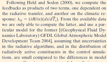
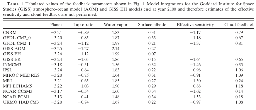
The primitive value is clearly not the right one. For it represents the change of emission temperature T_0 with ΔF0. But λ0 is defined (in Fig 1, for example) as the rate of change of surface temperature T_S with ΔF0. You cannot expect that these will be the same. In fact, if you simply multiply .267 by (T_S/T_0) you get 0.302, not so far from .313.
The proper version of this factor is given by Soden and Held (op cit)
For Planck feedback, x is T_0, and so what is required is a GCM estimate of ∂T_S/∂T_0, the correction factor to the primitive. That is found and used in their Table 1, which I have referred to before:
Note that S&H use an inverse convention; λ0 (Planck) is in W/m2/K. Just invert to get the MoB convention.
The account given by Mr Stokes amply confirms the point made in the head posting: lambda-zero is indeed being determined in the models as Schlesinger determines it: by reference to surface temperature set against emission-altitude flux. Yet the SB equation relates flux density and temperature at the same surface, not at distinct surfaces. Looks like an error to me.
It’s not an error, it the whole basis of the conceptual model that you have already used yourself (you fig 1) and that relates surface temperature changes to flux changes at the top of the atmosphere.
“Yet the SB equation relates flux density and temperature at the same surface, not at distinct surfaces. Looks like an error to me.”
No, it’s the factoristion that S&H set out.
λ0 = ∂R/∂x ∂x/∂T_S = ∂R/∂T_0 ∂T_0/∂T_S
∂R/∂T_0 expresses the change of R with T_0,( the 0.267 above). But the definition is change wrt T_S. To get that, you need the second factor, which GCMs can provide.
Still looks like an error to me. The change in surface temperature following a change in emission temperature is, to first order and assuming no change in lapse rate, identical to the emission temperature change.
“to first order”
Yes. They are looking for second order. As you noted, the ratio is about 7/6, not 1.
“Still looks like an error to me”
And this is very good news. What looks like correct for you is generally wrong.
Nick, thanks for posting table 1. The amazing thing to me is this. The models show a lapse rate feedback that varies by a factor of 3 from small to large. Three! Their water vapor feedback varies by about 1.5 to 1. Surface albedo feedback varies by 4.5 to 1 small to large. And cloud feedback varies by an astounding 7 to 1 from small to large.
Despite that, they all do relatively well at emulating the historical changes in temperature.
This is why I laugh when people claim that the models are based on “simple physics” and the like … what we are seeing are the marvels of having lots of tunable parameters. Yes, each of them can make the elephant wiggle his trunk …
So what?
And people actually believe that if you just average all of them together they can give us the evolution of the climate for the next century …
w.
“The account given by Mr Stokes amply confirms the point made in the head posting: lambda-zero is indeed being determined in the models as Schlesinger determines it: by reference to surface temperature set against emission-altitude flux. Yet the SB equation relates flux density and temperature at the same surface, not at distinct surfaces. Looks like an error to me.”
Try reading the methods section of Soden & Held (2006) and you should see why it is not an error.
Soden & Held (2006) show quite clearly that the original error made by Schlesinger is now set in stone in the models: they are incorrectly comparing surface temperature change with emission-surface rather than hard-deck-surface flux (the two are very different), and one effect of this ghastly mismatch is to treat part of the lapse-rate feedback as though it were part of the original forcing. Another is to allow a substantial overstatement of the reference sensitivity parameter and hence of all temperature feedbacks.
Peter and the lord
I have been visiting this site since very close to it’s inception. I never have and never will be a warmist. However, If I find, or feel, a friend or enemy could be mistaken about some detail, I will point it out to them.
I use Alex because that is my name, at no point did I feel it necessary to give more than that. I don’t see the need to give my full details and home address or credit card number. My email address is registered with this site and I can be contacted at any time by the runners of this site. There are a lot of loonies out there. Yes, I’m a little paranoid.
If you want some basic bio about me then here it is:
I am 67 and retired when I was 38. I make and invent things and do a lot of study in my area of interests. You won’t find any of my products on the market because I just make things for myself. I frankly couldn’t care less about money or improving the lot of humans on the planet.
This does not mean I’m some weird guy. I’m in a long term relationship and I have acquaintances around the world that think I’m very cool and have a brain the size of a planet.
So, because I am magnanimous, there is no need to apologise
Very good article as is the work done by David Evans from a different direction. Global warming/climate change is not science nor is it happening as predicted, it is very good to see it being challenged against the consensus by people not supported by floods of government money.
Martin Mason, have you read Soden & Held (2006)? A free pdf is here:
https://www.gfdl.noaa.gov/bibliography/related_files/bjs0601.pdf
Do you think there is something wrong with their radiative kernel approach? Could you be specific?
Your insistence on citing and posting links to ‘Soden & Held (2006)’ as responses to the calculations and questions of Lord Monckton’s article above are bizarre.
If you actually read ‘S&H 2006’ you would recognize some of the calculation problems cited by Lord Monckton above.
ATheoK, “If you actually read ‘S&H 2006’ you would recognize some of the calculation problems cited by Lord Monckton above.”
This blog post is nothing like Soden & Held’s approach, it seems clear to me that Monckton either hasn’t read it or he hasn’t understood it and his entire post borders not-even-wrong.
Perhaps you understand Soden & Held’s paper better than me, in which case I’d like to learn. Two starter questions:
1) what is the change in mean temperature of a the “effective radiation level” change when the surface temperature increases by 1 K in S&H’s calculation?
2) How does the “effective radiation level” change with wavelength, and how does the S&H method account for this?
MieScatter continues to duck the central question. The reference sensitivity parameter ought to be determined solely and wholly at the emission altitude, with the lapse-rate held constant (not all that far from observation, actually), so that any change to the lapse rate is treated not as part of the forcing but as part of the lapse-rate feedback. However, S&H make it quite clear that emission-surface flux and hard-deck surface temperature are the points of comparison, and that, therefore, there are different pre-feedback temperature changes at the surface and at the emission altitude. But that implies a change in the lapse-rate, which is not a forcing but a feedback.
Monckton of Brenchley: for a global-average surface temperature change of 1 K in the Soden & Held method, what is the change in the lapse rate when they calculate the Planck response?
Did anybody considered the hidden hypotheses behind the “forcing” concept?
1- the forcings are linear
2- the forcings are independent from each other
3- the forcings act immediately (without delay).
For more details and consequences, have a look at: https://dl.dropboxusercontent.com/u/56918808/forcings_rel%2001.08.pptx
Please note I did not discuss in details the value of the parameters, as done brillantly in this post. but my analysis remain valid, from a conceptual point of view
The CO2 forcing function is actually logarithmic.
You are absolutely right. But I referred actually and specifically to the denominator term 1-F = 1-sum(fi). Which means that the individual forcings just sum up: this is what I mean with “linear” and “independent”. For the “delay” (3rd hidden hypothesis), this simplification is of paramount importance. Delayed non linear equations become easily chaotic (dynamical systems). A simple example is the rather well known”logistic equation”: x(t+1) = a*x(t)*(1-x(t)). which is nothing else than the product of a positive and a negative delayed feedback (or forcing). If you “tune” the parameter “a”, you’ll find amazing properties. The equation leads to a result that becomes rather unpredictable and which is extremely dependent on the initial conditions and the value of the parameter (for values of “a” in the range 3.6 < <4). Transposed to climate science (?), this means that if the climate system behaves in the same way (and it can be proved mathematically that it exhibits a "chaotic signature"), all the "projections" you made are extremely dependent on the exact values of the parameters used for calibrating the model: the initial conditions resulting from time series of experimental data from the past (and the associated experimental and algorithmic errors) and from the parameters (the exact value of the sum of the individual forcings, for example). On those two issues "the science is NOT settled" as shown by the abundant recent (and peer reviewed if you believe this gives some credibility) literature on the subject, not to refer to the present post and discussion. It seems thus reasonable to me, based on purely mathematical considerations, to claim that the climate system is not predictable on the long term. Different methods do exist to predict the horizon of predictability from time series. The problem is, as you know, to get this kind of work applied to climate data published.
It is good to see a discussion of the chaoticity of the Verhulst logistical model here. Indeed, the climate is sensitive to minor perturbations in the initial conditions (see e.g., Lorenz, 1963; Giorgi, 2005; IPCC AR3, para. 14.2.2.2).
However, it will become apparent when I turn to the feedback side of the official climate-sensitivity equation that the feedback forcings do not come anywhere near as close to unity as the models currently imagine.
Henry Masson: “Did anybody considered the hidden hypotheses behind the “forcing” concept?”
Yes. One relatively recent example, among a large literature on the subject:
http://dx.doi.org/10.1088/1748-9326/10/10/104010
Many thanks Mike for this interesting reference. But at first sight, it does not address the third (and probably most critical) hidden hypothesis stating that feedbacks are instantaneous, while chaotic behaviour (and extremely limited predictability) is closely linked to delays in the feedback loops (=forcing), and that obviously such delays have been spotted in experimental data (800 years time constant of the “oceans” i.e.). Also a-periodic (= not exactly periodic) and intermittent fluctuations as observed in many time series are an indication of dynamical (= chaotic) behaviour.
Feedbacks are not assumed to be instantaneous, but it’s necessary to pick some way of differentiating between feedbacks and forcing.
Check IPCC AR5 Chapter 8 discussion on effective radiative forcing and on the fixed-SST and regression method for disaggregating forcing and feedbacks in models.
Many thanks for your suggestion and comments. But I am still puzzled, as the equation in 1/(1-sum(f_i)) is typical of and only valid for linear, independent and instantaneous feedbacks, as I recalled in the dropbox link given above, and that I recall for convenience: https://dl.dropboxusercontent.com/u/56918808/forcings_rel%2001.08.pptx
In answer to M Masson, the head posting does make it clear that, since we are dealing with equilibrium sensitivity, the non-linearity of temperature feedbacks is not an issue. However, an account of the treatment of non-linear feedbacks will be found in Roe (2009), freely available on the web.
Many thanks for the reference to the work of Roe. Please note however that he is considering “red noise” (Brownian motion) and not pink noise (following a 1/f law). The amplitude distribution of Power spectrums of most climate data (and other dynamical systems) exhibit generally a pink noise signature. Such a pink noise signature is even often considered as indicative of the existence of a dynamical system (i.e. when applied to visibility graphs)
In response to M Masson, Roe explicitly entitles his paper “red noise” and also explicitly refers to the G = 1 / (1 – f) amplification function for feedback factors.
… and Roe gives in his paper a sketch exhibiting clearly my three initial claims regarding the 1/(1-sum(f_i)): the feedbacks must be linear, independent of each others and acting without any delay. Otherwise the formula does not apply. And this jeopardizes the whole “forcing” paradigm. Also, coming back to a later comment I made on Roe’s paper: “red” noise refers to Brownian motions /data. “white” noise to purely random motions /data. “pink” noise refers to a “1/frequency” law. If you look at amplitude distributions and power spectra, you’ll find that many time series describing natural / ecological /socio-economic “concepts” follow such a kind of law. Climate data is not an exception See for example John Gribbin’s “Deep Simplicity, Chaos, Complexity and the Emergence of Life” (Allen Lane /Penguin books, 2004), and more precisely the chapter 5, for having a first overview on this.
“3- the forcings act immediately (without delay).”
This is irrelevant to the equilibrium sensitivity being discussed here. It describes the difference between steady states, without reference to the intermediate stages and their timing. For each such steady state, it describes the feedbacks that have become established.
You are right Nick, but the problem is that of course you never reach local equilibrium, as this requires an infinite time. The climate system is never “static”, as the Earth rotates around it axis and the incoming solar flux in each point changes thus continuously. Not to mention the even fast dynamics of clouds acting as a blanket (during the night) or a shutter (during the day). I think this is the basic flaw of the whole IPCC approach: they ignore the fact that the system is (far) away from equilibrium, even locally.
I am sorry to ask a really stupid question. Would somebody be kind enough to explain (or point me to a reference) how the all-important climate sensitivity can be reconciled to the concept of saturation whereby (as I understand it) the radiation at the relevant CO2-sensitive wavelength is all absorbed and (as I adduce) the sensitivity reduces to zero? The two phenomena seem to give quite different characteristics.
Since the CO2 forcing function is logarithmic, each doubling of concentration will increase radiative flux density by a fixed amount. At or near the Earth’s surface, the absorption wavelengths of CI2 are largely overlain by those of water vapor, but in the mid-troposphere there is still scope for some warming to be caused.
Surely the point is that CO2 absorbs all the radiation available to it at approx. 20ppm. Absorption on the shoulders of the absorption bands in the absence of water vapor should already be accounted for. At 400ppm there should be no more thermalization unless TSI increases.
Siamiam would be right as far as the surface is concerned, but the upper troposphere is drier, and it is here that the CO2 forcing begins to matter.
Monckton of Brenchley September 4, 2016 at 3:00 am
At or near the Earth’s surface, the absorption wavelengths of CI2 are largely overlain by those of water vapor, but in the mid-troposphere there is still scope for some warming to be caused.
Water vapor lines are rather sparse in the absorption region of CO2, see below for an example (top is CO2):
http://i302.photobucket.com/albums/nn107/Sprintstar400/CO2H2O.gif
Steve Borodin, does this help?
https://youtu.be/we8VXwa83FQ
MieScatter
September 4, 2016 at 9:40 am: Totally outed yourselves now, you lot. Trolls I’ve met before. Wreckers, but so predictable.
“he was applying the Stefan Boltzmann equation by straddling uncomfortably across two distinct surfaces in a manner never intended either by Jozef Stefan”
There is too much reliance in this post on the notion of an emission surface. There is no such surface at which the S-B law can be applied. There are not “two distinct surfaces”. Hansen describes his T_e as an effective radiating temperature from the Earth, which he derives from the formal S-B law. He does not claim that it is a temperature of any particular location, and of course emission comes from a whole range of values. Others do likewise. It is simply a parameter determining flux, and Soden and Held show how to use it. Differential dependence of flux on the parameter is easy; what is then needed is the rate of change of that parameter with T_S. That comes from GCMs.
At the mean emission altitude around 5.3 km a.g.l., the net flux density is 238 W/m2 and, given emissivity at unity, the equivalent temperature at that altitude is 254.5 K or thereby. Change the flux density at that altitude by 3.7 W/m2 and the temperature rises by 1 K.
At the surface, temperature is 288 K and, with emissivity at or close to unity, corresponding flux density is 390 W/m2. Change the surface flux density by 3.7 W/m2 and the surface temperature rises by 0.67 K.
At any SB surface in between these two, the reference-temperature change would be between 0.7 and 1 K. I see no basis for the conclusion that it would be more than that.
“given emissivity at unity”
But emissivity of what thing? Gas has an emissivity per unit depth, but it is far from unity. You can think of its Kirchhoff equivalent, absorptivity. Gas is not locally black. It may be that all incoming radiation of some wavelength will be absorbed somewhere in the air, so the whole earth looks like a black body. But there is no surface (in the air) that has absorptivity one.
T_0 is simply an analogy. It is the temperature that the Earth would have if it were a black body emitting that flux. But that doesn’t mean there is an actual black surface doing that. The point of such a parameter is that you can hope that T_S will behave something like T_0 as flux changes. In olden times, that was all they could do. But in IPCC times we can with GCM do what is required. That is to find the derivative of that parameter with respect to T_S. That is not in principle different to using the GCM to find λ_0 directly, but seems more natural, since ∂T_0/∂T_S is close to 1 – as you noted, about 7/6.
In fact, the coefficient 7/6, though it is implicit in the official method of determining lambda-zero, is inappropriate, because it arises from the improper use, ever since Schlesinger (1985), of surface rather than emission-altitude temperature as the denominator in the first derivative of the Stefan-Boltzmann equation.
Nick
I am a little puzzled by this ‘virtual surface’ thing. Is it some sort of mathematical construct with no basis in reality? I would ask the lord but he would probably tell me to read a book or quote some latin at me.
I have reasonable knowledge about fluxes etc. but I can’t for the life of me work out how you can establish an altitude where things balance. The downwelling and upwelling mix is different. There would also be latitudinal differences including the atmospheric mass. If you can’t explain briefly, then point me in a direction where It can be explained
Alex,
You can’t characterise such a surface as a flux neutral point. Total heat flux (steady) is the same at all altitude surfaces (changing slightly in intensity as the area expands with radius to centre). It is partitioned into SW, LW and convection, so you might find neutral points of some subset, but not well defined.
T_0 is just defined as (F/σ)^(1/4). F is a global average. T_0 is more often called effective emission temperature. And you can calculate a surface at which that would be attained (lapse rate), but it has no special properties. T_0 is the temperature at which a black body would emit F. The Earth isn’t black, but it is dark (for IR) so it is reasonable to think dependence on T_S might follow T_0. Lord M calls that “first order”. But it is a guess, and with GCMs you can really find out. That is what they do.
In reply to Alex (and overlooking the silly sneer in his tone), the emission surface of a planet with an atmosphere is the locus of all points at or above the hard-deck surface at which incoming and outgoing radiation are equal, since it is from that “surface” that outgoing radiation from the Earth is observed to emanate.
My contention is that climate-sensitivity calculations should be performed at the emission surface. However, Schlesinger (1985) adopted a novel notion – that a legitimate differential of the fundamental equation of radiative transfer could be obtained by taking the ratio of hard-deck surface temperature to emission-surface net radiative flux density.
This leads to a considerable overstatement of lambda-zero and hence not only of pre-feedback warming but also of each individual feedback.
The models have since found it expedient to emulate this questionable device, since otherwise climate sensitivity falls quite a bit.
As to “finding a balance”, it’s not too difficult. Since the emission surface is defined as I have defined it (or, rather, as Professor Lindzen has defined it, for it is his definition that I am using), the net flux density is known and the emissivity are known, from which the emission temperature can be calculated (either by a global mean or by latitudinal means), and, given the known lapse rate, the mean altitude of the emission surface (about 5.3 km a.g.l.) can be readily determined.
“In reply to Alex (and overlooking the silly sneer in his tone), the emission surface of a planet with an atmosphere is the locus of all points at or above the hard-deck surface at which incoming and outgoing radiation are equal, since it is from that “surface” that outgoing radiation from the Earth is observed to emanate.”
None of this makes much sense. Outgoing radiation is not observed to emanate from such a surface. It is the sum of emanation from various levels, influenced by frequency, including about 20% which comes direct from “hard-deck” in the atmospheric frequency window.
But the surface definition makes little sense. The net heat flux (averaged over time and area, and spectral frequency) at any level is equal to the small heat loss from Earth’s interior. At TOA, that means that incoming radiation (mainly SW) and outgoing IR are equal. Coming down to the troposphere, part of the upward flux is taken over by convection (and LH advection), so in general down radiation will exceed up.
And if you don’t average, you have a complete mess. Where is that locus at night? But while averaging is fine for accounting for conserved quantities like heat (hence temperature) it doesn’t make sense for defining a surface for radiation, which responds to current circumstances.
I think link to Lindzen is needed.
Monckton of Brenchley September 4, 2016 at 11:54 am
In reply to Alex (and overlooking the silly sneer in his tone), the emission surface of a planet with an atmosphere is the locus of all points at or above the hard-deck surface at which incoming and outgoing radiation are equal, since it is from that “surface” that outgoing radiation from the Earth is observed to emanate.
No, the ’emission surface’ model which you use is the equivalent black body emitter which emits the same flux as is received by the planet. Such a surface would be at a temperature of ~255K which in a standard atmosphere would at ~5.3 km. Such a surface does not exist and using it to calculate sensitivity etc. as Monckton does, given the nonlinearities involved, is inappropriate (especially if you’re doing so to claim that the detailed calculations are in error).
For example, in the tropical atmosphere (cloudless), CO2 emission near the peak of the emission spectrum at ~15microns is at ~220K ( 12.5km), the Q-branch spike is at ~35km. In contrast the ‘window’ region between 10 and 13 microns emits directly to space from the surface at ~300K. Add some stratus clouds around 1km and the emission from the cloud tops is at ~290K, add some cumulus and it drops to ~280K. All these effects are supposed to be accounted for by the assumed ’emission surface’ in Monckton’s model.
If “Phil.” wants to take up with the IPCC secretariat the issue of their using emission-altitude flux as part of the basis for their calculations, let him do so. However, the virtue of that approach is that the emission-altitude flux is easily measured by cavitometers on satellites.
From that flux, the emission temperature of the Earth – which is the temperature that it would possess at the surface if the surface were a blackbody and if there were no atmosphere and no change in today’s albedo – may be determined directly via the SB equation, and there is in fact a mean altitude at which that temperature obtains. It is about 5 km a.g.l.
Monckton of Brenchley says: ” the emission-altitude flux is easily measured by cavitometers on satellites.”
..
WRONG
..
http://www.bsuir.by/online/showpage.jsp?PageID=93100&resID=119941&lang=en&menuItemID=120098
…
Cavitometers do not measure emission flux.
Monckton of Brenchley September 5, 2016 at 4:34 pm
If “Phil.” wants to take up with the IPCC secretariat the issue of their using emission-altitude flux as part of the basis for their calculations, let him do so.
No I’m taking it up with you, because it is you, not they, who is misusing the concept in order to incorrectly claim that they have made an error. Note that any addition of CO2 will increase emission from ~12.5km (~220K).
The S-B relationship you use is the integral across all wavelengths of the Planck’s Law equation, in the case of the atmosphere where emission is from a variety of temperatures it’s appropriate to integrate using the actual temperatures at each wavelength. Using Line by Line calculations in the relevant parts of the spectrum as the models do. The average emission altitude is a simple means of illustrating the way the GHG effect works, given the non-linearities involved you can’t use it to accurately calculate the sensitivity.
I notice that you have made no attempt to address the error in your claim that:
“the absorption wavelengths of CI2(sic.) are largely overlain by those of water vapor”
Mr Baguley incorrectly asserts that I had stated that cavitometers on satellites measure emission flux. No: I said they measure emission-surface flux, for, by definition, the incoming radiation measured by the cavitometers is, at that altitude, equal to the outgoing radiation. See Lindzen’s talks on the definition of what he calls the “characteristic-emission altitude”.
Monckton of Brenchley, let me make it simpler so even you can understand.
..
Satellites don’t have cavitometers
..
Get it?
Particularly with respect to the long-wave radiation with which we are here concerned, the emissivity of the emission “surface” is as near unity as makes no difference.
as seen in another post of yours above, there is too much reliance on the output of various cfd modelers. the modeling of airflow over the surface of aircraft wings has yet to be perfected ,as evidenced by various stabilisers and airflow interruption devices attached post production in the test phase. the notion that any cfd model gets remotely close to accurately modeling the atmosphere is delusional in the extreme .
in the case of the cost to humanity in implementing measures to halt cagw, near enough is just not good enough.
I suggest you check out the contribution that Tony Jameson’s CFD modeling of wings has made to the redesign of wings, notably for Boeing and Airbus.
http://aero-comlab.stanford.edu/Papers/AirplaneDesignShanghai.pdf
The leader of the 737 Aerodynamics program stated: “Without the understanding gained from CFD there would not have been a 737-300 Program!
Well, this is all a bit irrelevant really:
https://www.theguardian.com/environment/2016/sep/03/breakthrough-us-china-agree-ratify-paris-climate-change-deal
And arctic sea ice extent at second lowest in the record.
Parts of the world which count recognise man made climate change and the evidence for it plainer than ever.
Even those pushing the Arctic sea ice meme realize this years low is the result of storms. The fact anyone would mention it in regards to man made climate change shows denial of reality. Have you always been prone to delusions?
As for the Paris agreement? It is not worth the paper it was written on as many AGW supporters realize. It has no teeth.
Griff,has been taken to school on this,on other websites and here too just recently. as you pointed out,hat powerful WIND driven storms for ALL three low years of 2007,2012 and 2016 were the main cause of low summer ice extent.
He also fails to account for the evidence that Arctic region have been mostly or totally ice free in the summer for many years,in the early part of the Holocene.
Richards M: “Even those pushing the Arctic sea ice meme realize this years low is the result of storms. The fact anyone would mention it in regards to man made climate change shows denial of reality. Have you always been prone to delusions?”
It seems that summer Arctic sea ice extent is the lowest in at least 1,450 years (Kinnard et al., 2011 http://dx.doi.org/10.1038/nature10581 ).
Did we get storms in the Arctic for the first time in 1,450 years?
“And arctic sea ice extent at second lowest in the record.”
Sounds impressive huh? But that’s a record which is only 35y long in a climate system which is known to have a strong circa 60y periodicity, which was at its coolest in in 1975 and peaked around 2005. I suspect that 2012 will be the trough of the ice cycle for the next few decades.
In 2007 we were told it is was “run away” melting , climate meltdown, death spiral etc. Then the canary in the coal mine started to feel better. In 2012 we had another OMG moment but in 2013 NH sea ice volume increased by 50% in a single year. WTF? That is more like a sign of a strong negative feedback.
Hardly compatible with the tipping point hyperbole. So alarmists suddenly went quiet about it for a couple of years and started bed-wetting about millennial scale “melt-down” in Antarctic.
Now they think the Arctic is worth bemoaning again but this time because it’s the lowest winter max. EVAH ( ie in the last 35y of the warm part of the AMO cycle ).
So what Griff the grifter probably needs to ask himself is why , after the lowest winter max EVAH we are only seeing the second lowest summer ice coverage. Odd that this ice which is has been subject to the worst AGW since the dawn of man is now melting so slowly that even starting at a low point in winter does not lead to a new summer minimum.
As for the much heralded “agreement” with China , it would be wise to see EXACTLY what POTUS says, when he actually does ( rather than the froth and lather that MSM are fluffing up before it actually happens ) and exactly now he intends to sign a treaty that he has no constitutional authority to sign.
IMO this will turn out to be a “joint statement” of intent with little substance and lots of puff.
MieScatter doesn’t appear to understand what “extensive uncertainties remain” means. He seems to think the paper he referenced is based on data. Face-palm. You need to go back to the turnip farm.
‘Kinnard et al., 2011’ use ‘high resolution land based proxies’ to postulate Arctic Sea ice in an area greater than 14-15 million square kilometers.
From their proxy analysis they find that the recent warming is consistent with anthropological warming influence.
Correlation does not mean causation.
A lack of definitive certification of proxy accuracy implies massive possibilities for errors. Definitely not a definitively accurate analysis.
Leaps to vague assumptions with the CAGW religious faithful promoting ‘consistent with’ to absolute certainty.
Translation: They haven’t solved any puzzles. The Inuit verbal history is still the best historical source until the satellite era began.
Rising greenhouse gases are modeled to increase positive NAO/AO giving a more northerly jet stream track. That can only cool the Arctic.
http://www.ipcc.ch/publications_and_data/ar4/wg1/en/ch10s10-3-5-6.html
The rational explanation for the increase in the negative NAO/AO that has driven the AMO and Arctic warming since 1995, is the decline in solar wind strength.
have a look the same time next year. all that open water is no longer insulated by ice ,resulting in much heat being lost to the atmosphere.
bit chilly, there’s some interesting work been done on this, including the importance of inversions. See e.g. Bintanja et al. (2011, http://dx.doi.org/10.1038/ngeo1285 )
At or near the Earth’s surface, the absorption wavelengths of CO2 are largely overlain by those of water vapor
Such sentences I have read nearly everywhere, just like those claiming that CO2 merely absorbs around 15µ and nowhere else in the spectrum.
I’m not a physicist and therefore can’t say by own knowledge wether or not it is correct. All I can do is to read papers and consult web sites informing about the topic.
To be clear: I’m not at all interested here about the relevance of CO2 as a GHG, but solely in obtaining a (scientific) comfirmation of (or contradiction to) what follows.
The first I have read is that Earth’s IR emission near its surface, with temperatures from say 35 °C in the Tropics till say -60 °C in Antarctica, should range from about 9.5µ up to about 13.5 µ. That’s what you are told when consulting
http://spectralcalc.com/blackbody_calculator/blackbody.php
Quite in the near you find
http://spectralcalc.com/spectral_browser/db_intensity.php
from which you obtain, for the wavelength range above, and selecting the default database (HITRAN2012)
http://fs5.directupload.net/images/160904/93kwvitf.png
1,741 absorption lines for H2O, and
http://fs5.directupload.net/images/160904/nvktqojl.png
27,100 for CO2 (note that selecting older material, e.g. HITRAN2004, gives less absorption lines for both gases: 603 for H2O resp. 3,214 for CO2).
This would mean that CO2‘s ability to absorb IR certainly is not less than that of H2O. Water vapor’s higher IR absorption would then solely be due to the fact that it is by far more abundant in the atmosphere (at least below 10 km).
So if somebody happened to read this comment and to exactly (!!!) know wether or not this assumption is correct, s/he should feel free to answer!
Omissions are inevitable as it seems.
It must be noted that the two plots above possibly give a distorted impression, as they have a logarithmic scale. Using a linear scale gives a different view.
H2O:
http://fs5.directupload.net/images/160904/iage4rwk.png
CO2:
http://fs5.directupload.net/images/160904/79njt5is.png
But I obviously don’t know the exact scientific interpretation of the difference.
Yes, and furthermore, half the smog of rotational lines they are fond of showing around the important vibrational lines are destructive and reduce the energy of the molecule. The “p” and “r” rotational lines are a couple orders of magnitude weaker than the central “q” vibration. The destructive “r” lines are a bit stronger than the constructive “p”, so the net effect of the rotational smog is a small loss of energy to the molecule.
Those are vacuum spectra plots for a single molecule. They change considerably at atmospheric pressure, temperate, and abundance. In the lower troposphere, about 50% of the CO2 spectra overlaps with water vapor. In the stratosphere, there is no overlap because water is only 5 ppm, it is 10,000 ppm in the lower troposphere.
Bindidon To apply this spectroscopic data, use quantitative Line By Line (LBL) radiation/absorption models. e.g.
Intercomparison of Far Infrared Line By Line Radiative Transfer Models Kratz et al. 2005
One of the models is HARTCODE by Ferenc M. Miskolczi as applied in Fig 2, Fig 4 and Fig 5 in
The Greenhouse Effect and the Infrared
Radiative Structure of the Earth’s Atmosphere 2014.
Thank you David L. Hagen, I have a pdf “First light from the Far-Infrared Spectroscopy of the Troposphere
(FIRST) instrument” on disk. The second link is very interesting though a bit harder to digest.
But what I’m looking for is rather to be seen in the context of publications like
http://newscenter.lbl.gov/2015/02/25/co2-greenhouse-effect-increase/
http://www.nature.com/nature/journal/vaop/ncurrent/full/nature14240.html
Suddenly I remember to have read this
http://www.drroyspencer.com/2010/08/comments-on-miskolczi%E2%80%99s-2010-controversial-greenhouse-theory/
years ago…
Thanks for the Co2 paper. Separate Miskolczi’s quantitative LBL from his first order equilibrium atmospheric modeling. Next need to add 2nd order issues to (and refine translation issues into English).
And… what about even this?
https://wattsupwiththat.com/2014/05/01/top-ten-skeptical-arguments-that-dont-hold-water/
??? Address the issues Spencer raised.
Robert Clemenzi on September 4, 2016 at 8:14 pm
Thanks.
They change considerably at atmospheric pressure, temperate, and abundance.
Spectralcalc has a radio button selector to activate a scaling by atmospheric abundance but this didn’t change anything. Maybe it’s behind their paywall.
Sorry, the red line not blue.
You have only shown a small part of the CO2 spectrum, the Earth’s IR emission covers ~5-25 microns, the 15 micron band is close to the energy peak of the emission.
You are right Phil, but the focus was here I guess on the IR emitted at surface.
HITRAN tells us that CO2 absorbs/emits even till 30µ, i.e. -150 °C or 23 km (probably the altitude where it emits to outer space).
HITRAN is just a catalogue of spectral lines, so a graph of that will produce just lines. in the real world the lines are not just lines, they are much broader and will mesh with other lines in the series. not only are the lines wider for all molecules, but water vapour is special in that it forms a continuum. see-
http://www.sciencedirect.com/science/article/pii/S0022285216300637
Blindinon, you are mistaken, the surface at 300K still emits way beyond 15𝝻m. If you look at the graph below (green line) you’ll see that for an surface at 300K the emission peaks at ~700cm-1 (~15𝝻m), this is where the CO2 absorption/emission occurs (see the blue line).
http://i302.photobucket.com/albums/nn107/Sprintstar400/rad05093716.gif
mobihci September 5, 2016 at 9:56 pm
HITRAN is just a catalogue of spectral lines, so a graph of that will produce just lines. in the real world the lines are not just lines, they are much broader and will mesh with other lines in the series. not only are the lines wider for all molecules, but water vapour is special in that it forms a continuum. see-
Where it says the following:
“Within the main absorbing regions, continuum absorption is generally dominated by spectral-line absorption”
Also the spectra I posted above show the broadened lines, not the line map that Blindinon showed.
the differences between the real world and the HITRAN models are quite vast. eg-
https://www.arm.gov/publications/proceedings/conf09/extended_abs/mlawer_ej.pdf
we are talking about percentages here anyway, not absolutes. the abundance of water vapour more than makes up for the lack of specific lines. the fact that some frequencies are not absorbed means little when the effect of absorption has already taken place from another frequency on that specific molecule. co2 has no chance to make a difference in the lower atmosphere. where water vapour has a lower concentration higher in the atmosphere, then individual spectral lines become more important.
mobihci September 6, 2016 at 8:03 am
the differences between the real world and the HITRAN models are quite vast. eg-
https://www.arm.gov/publications/proceedings/conf09/extended_abs/mlawer_ej.pdf
we are talking about percentages here anyway, not absolutes. the abundance of water vapour more than makes up for the lack of specific lines. the fact that some frequencies are not absorbed means little when the effect of absorption has already taken place from another frequency on that specific molecule. co2 has no chance to make a difference in the lower atmosphere. where water vapour has a lower concentration higher in the atmosphere, then individual spectral lines become more important.
As your own reference says the continuum spectrum is very weak compared with the line spectrum.
Below is the CO2 spectrum (HITRAN) for the first 10m of the atmosphere at 400ppm and the H2O spectrum at 1%.
http://i302.photobucket.com/albums/nn107/Sprintstar400/CO2.jpg
http://i302.photobucket.com/albums/nn107/Sprintstar400/H2O.jpg
Well I know nothing about these calcs, but I can feel temperature changes like any animal on the planet. The Sun and water rule. No co2 effect of note exists because its too evenly distributed to explain the huge localised temperature differences – longitudinal, latitudinal and altitude. As for lapse rates, that changes too – check out ozone layer charts. While your at it look closely at Antarctic vortex compared to Arctic vortex. some really neat stuff happening with NOx destruction and heating variability during winters being greater than summers. Forget CO2 and subsequent sensitivity calcs. They are a fools errand and irrelevant. moot.
Thanks to Christopher Monckton and the other contributors to this thread. This back and forth, is the way things are eventually figured out. Very healthy for science.
I would like to commend Christopher Monckton for his patience in the face of provocation, and would like to request that all who diagree with him, do so without being disagreeable.
Personal attacks smack of desperation.
But it would seem that rebuttals of the good lords personal attacks, even without expletives, are not permitted on this site. Apparently there is no right of reply here. No censorship on this site. HAHA
[???? .mod]
Though I’m not always 100% happy with moderation here I would not say I see any censorship. Maybe you have something specific you wish to cite rather than such meaningless blanket accusations.
HAHA, indeed. Very funny. Now if you have something specific …
Alex,
You’re not making sense. Just because you believe something to be true, that doesn’t make it true.
You say there’s no right of reply—in your reply. Think about it.
My reply didn’t appear higher up in the thread. I was accused of being a CAGW person. When I responded, nothing happened ie appeared and disappeared. I made other comments later to other people,and they appeared. I’m not bothering with repeating what I said to the lord.
Perhaps it was one of those comments that disappear because of a glitch- in which case I apologise to the mods.
I don’t wish to discuss the matter any further.
I checked the spam que and banned words moderation filter que, and it is not in either of those. I suspect it never got submitted. It happens sometimes. It may also have something to do with the fact that your IP address says you are in China. It may be that the “great firewall of China” didn’t allow your post to be submitted in the first place.
Is this what you submitted at 6:21 AM here? If so, it seems to have gone through. Maybe you just didn’t refresh/scroll.
Since all your other posts got through it is likely that you used a banned word. This may be quite innocently. Don’t make sweeping conclusions from one post going missing.
“I don’t wish to discuss the matter any further.”
Very wise. At least we see you are not being censored as you had imagined to be the case.
“Thanks to Christopher Monckton and the other contributors to this thread. This back and forth, is the way things are eventually figured out. Very healthy for science.”
This stuff was worked out years ago, Christopher Monckton just hasn’t understood how the calculations were done, see e.g. Soden & Held (2006).
Scientists are now working on far more advanced details to improve these calculations further. They tend to do this in the peer-reviewed literature and conference proceedings rather than blogs though.
This stuff may have been worked out years ago, but some of it was worked out wrongly years ago and has remained wrong ever since.
… but some of it was worked out wrongly years ago and has remained wrong ever since
But where did Mr Monckton of Brenchley manage until now to give us any scientifically unfalsifiable proof of that?
“This stuff may have been worked out years ago, but some of it was worked out wrongly years ago and has remained wrong ever since.”
You’ve pointed out what you think is wrong with an introductory level model that scientists already know is oversimplified and gives a different result from full calculations.
Do you agree that the Soden & Held method directly answers the question: “what is the global-mean change in net flux at the top of the atmosphere when surface temperatures change by an average of 1 K?”
MieScatter continues to miss the central point I am making, which is that the determination of the reference sensitivity should be performed solely at the emission altitude, so that, with the lapse-rate held fixed, the temperature change at that altitude is the temperature change at the surface. Then, any lapse-rate changes that might occur as a result of the reference temperature change are correctly treated as part of the lapse-rate feedback. But that is not the regime described by Soden & Held, now, is it?
Monckton of Brenchley: you’re claiming that Soden & Held change the lapse rate. They don’t, read the Methods section.
Do you accept that the lapse rate is held constant?
“But that is not the regime described by Soden & Held, now, is it?”
What S&H describe in their Methodology is nothing like what you have been saying. Here it is:
They aren’t dealing with a supposed emitting surface. They aren’t even using a global effective emitting temperature. Using the GFDL GCM grid, they vary the temperature level by level, and that gives them the rate of change per that level k. That is the radiative calculation, and as per their factorisation, it does not need to be done over a long period. Then they take the long term GCM results and subtract the century difference (2110-2100 from 2010-2000) and that gives the climate rate of change of T_k relative to T_S. That gives a complete representation of the effects of temperature at different levels on surface, and gives the information needed to separately determine λ₀ and λ_L, according to the partitioning described thus:
Two distincts methods,
same answer.
So now, lets take a look at the last figure.
(CRF is … CRE)
Mr Stokes can wriggle all he wants, but Soden and Held’s values for lambda-zero make it quite plain that they are not determining those values either from the surface flux and temperature or from the emission-surface flux and temperature 5 km further up. They are are taking flux from further up and temperature from the surface. That is not a correct implementation of the SB equation, and it leads to a considerable and erroneous exaggeration of climate sensitivity.
“Mr Stokes can wriggle all he wants, but Soden and Held’s values for lambda-zero make it quite plain that they are not determining those values either from the surface flux and temperature or from the emission-surface flux and temperature 5 km further up. They are are taking flux from further up and temperature from the surface.”
Not wriggling – I’m actually reading the paper to find out what they did. You should try it. I thought at first that they used an average change T_0 and multiplied it by a derivative of F wrt that average. Approximating the average of the product with the product of the averages. But they did the correct thing of working out the product for local cell/time combinations where temperature could be assumed uniform, and averaging those products. As you note it gives a similar result. Using the product of averages for average of products is unreliable, but often does work out the same, as here.
In reply to Mr Stokes, here is what Soden & Held actually say they are doing:
“We define feedbacks in terms of the change in global mean surface temperature T(s) and the change in radiative flux at the top of the atmosphere (R).”
That approach, which derives from Schlesinger (1985) as explained in the head posting, is an abuse of the fundamental equation of radiative transfer, in which the feedbacks should be defined in terms of the changes in temperature and in flux density at the same surface and not at different surfaces.
“here is what Soden & Held actually say they are doing”
That is not what “they are doing”. It’s the definition of feedback and sensitivity. Everyone’s definition. From the AR5 glossary:
It’s just relating two separate quantities. There is no reason why they should be measured at the same place.
Monckton of Brenchley September 4, 2016 at 3:26 pm
MieScatter continues to miss the central point I am making, which is that the determination of the reference sensitivity should be performed solely at the emission altitude, so that, with the lapse-rate held fixed, the temperature change at that altitude is the temperature change at the surface. Then, any lapse-rate changes that might occur as a result of the reference temperature change are correctly treated as part of the lapse-rate feedback.
Well the emission altitude of CO2 is about 12.5km (T=~220K) so in order to determine the sensitivity to added CO2 why don’t you determine it there?
Phil: “Well the emission altitude of CO2 is about 12.5km (T=~220K) so in order to determine the sensitivity to added CO2 why don’t you determine it there?”
The feedbacks are separated from forcings, so that bit doesn’t matter.
You’re right that the “emission altitude” changes: at different altitudes it’s dominted by different gases or, in the window channels, the surface, which is why Soden & Held did the calculation the way they did. They account for a uniform warming up through the atmosphere, holding everything else constant (including the lapse rate, despite Monckton’s confusion).
If you look at their figures you can see that they include contributions from every level of the atmosphere, which is what you would get for a change in temperature. They also account for absorption above each layer of the atmosphere, which is what happens in the real world but not in Monckton’s introductory level equation.
Their calculation involves accounting for how absorption and emission depend on frequency and the abundance of emitters. It involves solving the full radiative transfer equation accounting for Planck’s law, because the loss of information from integrating it to the Stefan-Boltzmann equation means you can’t get the right answer for a nonuniform, spectrally-dependent case like the real atmosphere. Despite what Monckton says.
A comment at Nick Stokes’ blog shows that if the layer around 500 hPa (Monckton’s “emission surface”) warms by 1 K, then top-of-atmosphere emission changes by about 0.3 W m-2. The rest of the 2.8 W m-2 comes from other altitudes, including CO2 emission higher up.
MieScatter September 6, 2016 at 7:42 pm
Phil: “Well the emission altitude of CO2 is about 12.5km (T=~220K) so in order to determine the sensitivity to added CO2 why don’t you determine it there?”
The feedbacks are separated from forcings, so that bit doesn’t matter.
You’re right that the “emission altitude” changes: at different altitudes it’s dominted by different gases or, in the window channels, the surface, which is why Soden & Held did the calculation the way they did. They account for a uniform warming up through the atmosphere, holding everything else constant (including the lapse rate, despite Monckton’s confusion).
Yes, I know, I was trying to get Monckton to see the error of his ways (fat chance)!
You know, I think you’re right, Monkton is in error. No matter which way I do the math I get less than 0.18 for sensitivity. If I do it linearity I get about 0.13, if I do it from instrument malfunction I get a 0.06 , if I look at from Mt Pinatubo it’s, 2 w/m^2 and a 0.3 C drop makes, it 0.15 sensitivity. And if I do it from the real w/m^2 incoming 238 and out going at 235 that’s a big difference at calculating it 242 w/m^2, a drop of about 5 w/m^2. Which is an over estimation of about 0.7 C from Pinatubo, and a 0.65 from doing it from linear, drop from instrumention of about 0.3 C , and if we use the IPCC number of 0.6 about 3.0 C . I don’t know, you choose which story you want to tell. You tell me looking at what the modeled increase in temperature should have been, and the real world increase in temperature?
Let me be clear on this, I’m just playing along with your numbers. I actually think that co2 climate sensitivity is so low that’s it’s background noise.
Many thanks to TA for his kind words.
” 2. One or two commenters have suggested that the Stefan-Boltzmann calculation should be performed entirely at the hard-deck surface when determining climate sensitivity and not at the emission surface a mean 5.3 km above us. Professor Lindzen, who knows more about the atmosphere than anyone I have met, takes the view I have taken here: that the calculation should be performed at the emission surface and the temperature change translated straight to the hard-deck surface via the lapse-rate, so that (before any lapse-rate feedback, at any rate) ΔTS ≈ ΔT0. This implies λ0 = 0.264 K W–1 m2, the value taken as normative in Table 1.”
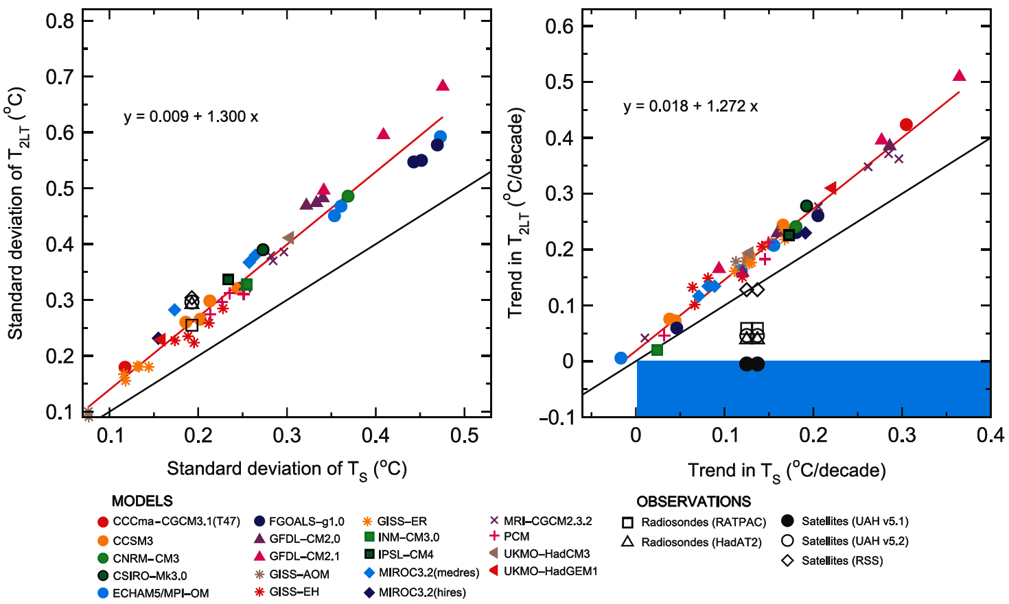

I was one of those.
Why? Because the Lapse Rate feedback is WRONG in the theory.
IPCC AR5 has bumped up the lapse rate feedback from -0.6 W/m2 (in AR4) to -0.9 W/m2 (in AR5). This signals that the “lapse rate’ will decrease from 6.5 C/km to about 6.3 C/km in the short medium term.
LR in this table.
http://jo.nova.s3.amazonaws.com/graph/atmosphere/hot-spot/ipcc-ch-9-feedbacks-a.gif
This means that they are predicting the “surface” will warm less fast than the troposphere shown in this graphic. The negative lapse rate feedback here.
The actual value is that the troposphere will warm by 1.3 times more than the surface. This is from Thorne 2011. The trend at the 2LT (the level of UAH and RSS satellites) should warm by 1.3 times that the surface in the climate models. We used to describe this as the “tropospheric hotspot”
But the “opposite” is actually happening.
The troposphere is warming less fast than the surface. The Lapse Rate feedback is not “negative”, it is positive. The Lapse rate has actually changed from 6.5 C/km to 6.6 C/km since 1979.
In other words, throw out the lapse rate feedback and move everything back to the surface where we live.
Sorry, I meant to say “IPCC AR5 has reduced the lapse rate feedback to -0.6 W/m2 (in AR5) from -0.9 W/m2 (in AR4).
Bill Illis makes an interesting point. Similar points could be made about the other individual feedbacks, in which there is both an inter-model spread and an inter-ensemble spread.
There is growing evidence, for instance, that the water vapor feedback is not occurring at all (see NOAA’s water vapor project graphs for the past 30 years, or those of ISCCP). Therefore the lapse-rate feedback, which originally depended in no small measure on the models’ now proven-incorrect assumption that the tropical mid-troposphere would warm at twice or even thrice the tropical surface rate, is going to have to be scaled back.
Frankly, all of the official climate-sensitivity calculations are a mess. And just watch out for the revelations yet to come.
While the surface temperature measurements (GISS, NOAA, HadCRUT4, BEST) grossly agree, with the exception of JMA being a bit cooler, we actually experience stronger differences between UAH6.0 and RSS4.0 (for which the TLT variant still is not in op).
We can’t compare them using Paul Clarke’s WFT, but when using RSS3.3 TTT which is here nearly identical to UAH6.0beta5, we can do it very well at Kevin Cowtan’s trend computer, from 1979 till present:
– RSS3.3 TTT: 0.123 ± 0.060 °C/decade (with TLS insemination)
– RSS4.0 TTT: 0.176 ± 0.061 °C/decade (TLS insemination reduced)
By comparing that with
– GISS l+o: 0.171 ± 0.040 °C/decade
we see that both surface and troposphere would seem to warm quite similar in case of RSS4.0 being over the long term the more correct appreciation for tropospheric temps. Wait and see.
wait and see ? for how long should we wait and see.
for how long should we wait and see.
At least as long as
– Remote Sensing Sytems needs to publish RSS4.0 TLT;
– experts manage to compare peer-revied papers from UAH and RSS.
The latter point has recently become more and more possible.
Please compare
http://www.drroyspencer.com/2016/08/uah-global-temperature-update-for-july-2016-0-39-deg-c/
hinting on
Note we are now at “beta5” for Version 6, and the paper describing the methodology is
still in peer review.
with
http://www.drroyspencer.com/2016/09/uah-global-temperature-update-for-august-2016-0-44-deg-c/
hinting on
Note we are now at “beta5” for Version 6, and the paper describing the methodology is
back to the journal editors from peer review.
That needed well oh well a lot of time.
The analysis does not change when observations do not support the theory in question. Paradoxes and anomalies occur when a theory is incorrect.
The troposphere is warming less fast than the surface and (I repeat, AND) the majority of the warming that has occurred is occurring at high latitude regions. Global warming is not global. It is latitude specific. As atmospheric CO2 is evenly distributed in the atmosphere the change in forcing for an increase in atmospheric CO2 should cause global warming, not latitude specific warming.
P.S.
The upper troposphere has cooled which is caused by less reflected sunlight off of clouds. The incoming sunlight and reflected sunlight warms the upper troposphere due to absorption of ozone.
Latitudinal specific warming (as opposed to global warming) and the fact that the troposphere is warming less fast than the surface along with satellite data (cloud cover has decreased in high latitude regions) in peer reviewed papers supports the assertion that the warming in the last 150 years was caused by changes in cloud cover, not due to the increase in atmospheric CO2.
There are cycles of high latitude warming and cooling in the paleo record (both hemispheres) which correlates to solar cycle changes.
The lapse rate in the troposphere is definitely increasing, as you say. Whether we should count only the surface not so sure.

Here is modtran looking up and down from the reputed mean ERL of 5.3 km:
It is very interesting that at this altitude up and down CO2 band intensity matches the altitude exactly, but no other ghg’s do. Despite the intensity/altitude match, the CO2 up and down fluxes are still wildly out of balance. Such balance takes place about 8km.
Yet unless one is arguing for emergent effects, we are talking about adding more CO2, pure and simple. The ERL of the CO2 bands is not 5.3km and it is not 8km. It is above 13km in that little vertical zone where the temperature ceases to “lapse” with altitude altogether, and above which it increases.
Bill Illis: Why? Because the Lapse Rate feedback is WRONG in the theory.
Thank you for your comment.
“The troposphere is warming less fast than the surface. The Lapse Rate feedback is not “negative”, it is positive. The Lapse rate has actually changed from 6.5 C/km to 6.6 C/km since 1979.”
How did you match up modelled layers to the MSU kernels? What are the uncertainties in your values?
Less divergence with SST’s only, but it’s still just there:
http://www.woodfortrees.org/graph/uah6/from:1979/plot/hadsst3gl/from:1979/plot/uah6/trend/plot/hadsst3gl/from:1979/trend
OK. I try to read everything you write here at WUWT Lord Moncton. I just finished this article.
1) are the computer models used by the UN still using James Hansen’s 1984 value? 1.2-1.3 K ΔT0=1.2-1.3 K ? I assume they are using the linear model as well.
2) The sensitivity equations that you propose is insufficient to align historical predictions of now to now data correct? So the sensitivity gap is a contributor to the overall error between the prediction and observed T?
finally 3) “committing suicide in despair at his own failure to convince the world of the existence of atoms”
I hope you don’t suffer such a thin skin! 🙂
In answer to Mr Westhaver, whom I congratulate on struggling through the rather detailed head posting:
1) The models are indeed using (or, at least, in their manner of operation reflecting) a reference sensitivity parameter lambda-zero that is equal to 0.3125 K/W/m2, which, when multiplied by the CO2 radiative forcing 3.708 W/m2, gives a reference or pre-feedback warming of 1.2 K, in line with Hansen’s 1.2-1.3 K. In truth, this value should be just under 1 K.
In answer to Mr Westhaver’s further questions:
2) Since my results will show climate sensitivity to be considerably below the current official estimates, there is of course a far better correspondence between prediction and reality in my model than in that of IPCC.
3) I have no plans at present to commit suicide, since I am far too interested in watching world events unfold.
Thank-you Lord Monckton of Brenchley. I pray that James Hansen suffers a dream like Nebuchadnezzar, that his gold head will be subject to his feet of iron and clay.
“1) are the computer models used by the UN still using James Hansen’s 1984 value? 1.2-1.3 K ΔT0=1.2-1.3 K ? I assume they are using the linear model as well.”
No. The Methods section here explains the Soden & Held (2006) calculations:
http://citeseerx.ist.psu.edu/viewdoc/download?doi=10.1.1.444.1470&rep=rep1&type=pdf
The calculation is nothing like the simplified equations shown in this blog post. For example, this equation is solved at every level in the troposphere at each location on Earth:
https://en.wikipedia.org/wiki/Radiative_transfer#The_equation_of_radiative_transfer
MieScatter uses a device common among unquestioning defenders of the Party Line: that the models are complex and therefore more likely to be right than the analysis here, which is simple. If, as he now says, radiative-transfer calculations are done at each altitude in the troposphere, then the mid-troposphere value for the first differential of that equation would be approximately the right value. Certainly all values for altitudes below the emission altitude of around 5 km would be lower than the value for that altitude.
Like it or not, the models assume a value for lambda-zero that is contrived from surface temperature and emission-altitude flux. That is what Soden and Held say is going on. That is what Schlesinger (1985) says is going on. That methodology is erroneous and leads to a considerable overstatement of climate sensitivity.
Regarding the surface equivalent of Equation 5 yielding a pre-feedback climate sensitivity of .192 K W^-1m^2 or .192 K / (W/m^2): That is .192 degree per 1 W/m^2 change in solar radiation alone. But this causes a change in outgoing longwave radiation from the surface, some of which is absorbed by greenhouse gases aloft and radiated back towards the surface. So the climate sensitivity before effects of albedo change, change of lapse rate, change of water vapor concentration, etc. (which are what are usually counted as feedbacks) is substantially more than .192 K W^-1-m^2.
In answer to Mr Klipstein, the sensitivity calculation is properly performed at the emission altitude, where the change in radiation is represented by a change in temperature, giving around 0.264 K/W/m2, which is indeed substantially more than 0.192; though there is a good case for saying that the latter value rather than the former should be used in feedback calculations (though this is not a case I shall be making here).
There is some uncertainty with regards to the lapse rate. This uncertainty and its effect on heat flux is also interconnected with clouds, especially in the lower troposphere(low clouds/cumulus). Increasing surface temperatures and dew points without an equivalent increase aloft, will steepen the lapse rate(positive feedback). This in turn, should lower the LCL(lifting condensation level) and result in more cumulus, especially those that form from rising air as a result of solar radiation heating the surface.
This in turn creates a negative feedback from cumulus forming earlier in the day and covering more of the daytime sky, blocking the more powerful SW radiation from reaching the surface. A positive contribution from trapped LW radiation takes place, which at night is the main effect from clouds.
There are a number of complicating factors that contribute to moisture and clouds. A greening of the planet has increased evapotransiration. A massive draw on aquifer/under water brought to the surface as well as other major regional changes in vegetation from crops and deforestation, ocean evaporation and changes in soil moisture from regional precipitation/weather changes.
These all have an effect on lower level moisture, which in most cases is a positive contribution. The real world effect should be and is verifying as a decrease in the diurnal temperature spread………positive effect on temperatures at night, negative during the day. Record warmth for nighttime temperatures is far exceeding new record highs in fact.
So how much of this is a contribution from the increase in water vapor seen as a positive feedback by itself in the models and how much is this effected by the changes in clouds?
Let’s say that we could in fact represent the lapse rate accurately with the right equations in the models………..in a cloud free atmosphere. The effect of cloud changes on heat flux, by themselves could be as great as the difference between the values being used to represent the lapse rate.
But then, low clouds, will greatly effect the lapse rate. Parcels rising at the moist adiabatic rate will have a different lapse rate in clear air, that is able to entrain drier air and result in a less than moist adiabatic rate than those that are in a deep cloud with a different entrainment dynamic after condensation.
These differences cannot be modeled.
I should adjust that to: some of these differences can’t be accurately represented as they are/will be occurring in the atmosphere in models(you can model anything).
Mike McGuire: There is some uncertainty with regards to the lapse rate.
That was a good comment. Thank you.
Would you happen to know who first wrote that cloud cover would be increased early in the day, causing a subsequent reduction in SW radiation to the Earth surface?
“who first wrote that cloud cover would be increased early in the day, causing a subsequent reduction in SW radiation to the Earth surface?”
Meteorology 101………..sort of. However, there are so many complicating factors………latitude and time of year for instance. Lows clouds in the higher latitudes, where the sun angle is low would not reduce SW radiation as much as in the tropics.
During Winter, when there is very little SW radiation to block, low clouds would serve mainly as trapping outgoing LW radiation in the higher latitudes.
This is consistent with observations of more warming in the coldest months of the higher latitudes.
Low clouds in the tropics would block enough SW radiation to cool the surface more. On balance, over the entire planet, what does this leave us? For sure less of a meridional temperature gradient. Then, with less of a horizontal temperature gradient in the atmosphere there is an effect on the movement of heat from areas of excess to areas of deficit.
The assumption that I am making based on 34 years as an operational meteorologist is that, with all else being equal(vertical velocities/lift for instance) regionally, if you add moisture to the air mass, whether it be from increased evapotranspiriation from a massive, densely packed corn crop in the Midwest or from a recent, widespread rain event over a large region, the lifting condensation level will be lower………moisture will condense out at a higher temperature/lower altitude and earlier in the day.
On a planetary scale, increasing water vapor should also do this. More low level cumulus clouds at the very least.
Then, there’s the contribution to increases in precipitation micro-physics that Dr. Spencer understands better than me:
http://www.drroyspencer.com/2014/09/water-vapor-feedback-and-the-global-warming-pause/
Related to just the US Cornbelt in the growing season, this is an interesting discussion about how corn evapotranspiration has created a “micro-climate”
https://www2.ucar.edu/atmosnews/perspective/4997/corn-and-climate-sweaty-topic
Christopher Monckton of Brenchley, thank you for your essay, once again.
Christopher Monckton of Brenchley, I also appreciate your informative replies to the critical comments. I think that the interchanges are mostly illuminating. I look forward to the next in this series.
Many thanks for your kind comments.
Nick Stokes
September 4, 2016 at 3:28 am
Thanks Nick. So that makes λ0 and output of the models. So is it also an input parameter as CoB is suggesting?
Greg,
No, GCMs do not use notions of feedback at all. I supported your view of that point here
Mr Stokes is being disingenuous. The models are constructed in such a way as to embody the mechanisms of feedback, though the feedbacks themselves are not stipulated as inputs. However, precisely because the models embody feedback mechanisms (such as, for instance, the water vapor feedback), it is possible for papers such as Soden & Held (2006) and Vial et al. (2013) to discern the values of the feedbacks from the models. See also AR5, fig. 9.43a, where the feedbacks thereby deduced are illustrated by IPCC.
“though the feedbacks themselves are not stipulated as inputs”
No you are being diseneguous MoB as is you usual want
As Nick Stokes says and which you do in your usual around the houses non- answering *refutation* – the feed-back parameter in the models is an emerging property of them. It drops out at the end. Not imputed AS A NUMBER at the start.
Which is what you do, and is non-physical.
That can actually be decoded as an admission when descrambling your wordage.
Look, just say it out loud my Lord, even the plebs know that honesty is what maketh the man.
toneb says it “drops out at the end”. how apt.
Toneb contributes nothing useful to the discussion. As will become apparent when I eventually reach the argument about feedbacks – which has not yet been covered in this series – there are some grave errors in the models’ handling of feedbacks. These errors are errors regardless of whether feedback values are input into the models or deduced from their output.
At its simplest, the warming without feedbacks is about 1 K. Any model that predicts equilibrium warming of more than 1 K contains routines that – by whatever method – take account of the existence of temperature feedbacks. At present, it is the view of the climatological community that there is an appreciable risk of feedback values elevated enough to cause even as much as 10 K global warming per doubling of CO2 concentration. Once I get to the argument about feedbacks, I shall demonstrate that any such conclusion is based on a large error in the determination of feedbacks. Take away the error and the probability of very high warming in response to doubled CO2 becomes vanishingly different from zero.
Toneb, in attempting to attack my argument on the feedback question before I have made it, is indicating prejudice.
Lord Monkton
Why do you respond so agressively to ToneB when all he has done is respond to your comment about feedback?
As a reminder, you said to Nick Stokes “The models are constructed in such a way as to embody the mechanisms of feedback, though the feedbacks themselves are not stipulated as inputs. However, precisely because the models embody feedback mechanisms (such as, for instance, the water vapor feedback), it is possible for papers such as Soden & Held (2006) and Vial et al. (2013) to discern the values of the feedbacks from the models. See also AR5, fig. 9.43a, where the feedbacks thereby deduced are illustrated by IPCC.”
” there are some grave errors in the models’ handling of feedbacks”
Again, GCMs do not handle feedbacks. They solve on a grid locally equations involving conserved quantities (radiation is a bit different). Feedback is a diagnostic tool. You try to fit the GCM results to a conceptual model of the way you think it ought to work. If you find that unsatisfactory, it may indicate a model failing. But also your fitting may have gone wrong, or the conceptual model may be inappropriate. Here the model seems at least over simplified.
Mr Stokes continues to be disingenuous. Of course the official climate-sensitivity equation that I have presented is simple: and yet, when calibrated against the models’ outputs deduced in Soden & Held (2006) and in Vial et al (2013) and encapsulated in AR5 (fig. 9.43a), it reproduces the published CMIP3 and CMIP5 exactly. So simplicity is not a hindrance to the purpose of the simple official equation, which is presented in the documents of IPCC. If Mr Stokes does not like the equation, let him address his concerns to the IPCC secretariat.
Now, either the models do contain routines that in some fashion allow for the existence and approximate magnitudes, in which event the simple equation (1) in the head posting will faithfully reproduce the feedbacks officially deduced from their outputs, or they do not, in which event they will simply predict the reference warming with no effect from feedbacks.
In fact, the warming they predict is plainly substantially greater than the reference warming, from which it is not rocket science to deduce that they contain processes and routines that reflect feedbacks. There is a very considerable literature on this: indeed, AR5 mentions the word “feedback” more than 1000 times.
Once the simple equation (1) has been calibrated against the models’ oficially-published outputs and has been found to reproduce their intervals of predicted climate sensitivity more or less exactly, it is then possible to examine various errors in the magnitudes of the variables or in the methods used, in order to find out what sensitivities would have emerged from the same simple equation (1) – amended where necessary to eradicate the errors.
That is a perfectly logical exercise; and, when all the errors have been revealed and discussed, those who have sworn blind that there are no errors may find themselves compelled to think again, and the architecture of the models is – in at least one major respect – going to have to be revised quite substantially. But more of that later in the series.
So far, I have established that even quite minor errors in the official methodology lead to quite large overstatements of climate sensitivity.
Similar explorations: Common errors in the use of the Stefan-Boltzmann equation Jinan Cao 2012
It’s remarkable that Germanic philosophers like Ernst Mach doubted that atoms existed as late as 1906, at least, yet British experimental physicists had already shown that not only atoms but subatomic particles indubitably exist. J. J. Thomson, for instance, demonstrated the existence of electrons in 1897.
It’s telling that Boltzmann was heavily influenced by British science, in particular Charles Darwin, and of course John Dalton, father of modern atomic theory, who died the year Boltzmann was born.
Many thanks to those who answered my earlier question. My area of ignorance is appropriately reduced.
As for an effective surface emissivity based on outgoing IR to space and surface temperature: I don’t think that is an incorrect concept, and here’s why:
Given IR leaving the planet and its atmosphere at 238.175 W/m^2 and an effective temperature at the effective radiating altitude being 254.578 K, surface temperature 288 K, surface emissivity being .96, and the surface radiating 374.503 W/m^2: This means the 238.175 W/m^2 of IR going to space (some from the atmosphere rather than the surface) is 63.6% of what the surface radiates, or 61.1% of what the surface would radiate at 288 K if its emissivity was 1.
Suppose solar output increases enough to cause the amount absorbed by the earth and the atmosphere to increase by 1 W/m^2 from 238.175 to 239.175 W/m^2. Assume absorptions and emissivities of the earth and the atmosphere don’t change, and the spectral shift of the IR radiation is negligible. The ratio of IR radiating to space from the earth/atmosphere to IR radiating from the surface would be unchanged at .636 (63.6%).
239.175/238.175 is a .41986% increase in W/m^2, so accomplishing this and maintaining equilibrium requires a temperature increase of .1048%. With ratio of radiation intensity from the surface to radiation intensity going out to space unchanged, the surface temperature also increases by .1048%. The temperature at the effective radiating altitude would increase from 254.578 to 254.8448 K (.2668 K increase), and the surface temperature would increase from 288 to 288.3018 K (.3018 K increase).
This does not require an increase of the lapse rate, because the part of the atmosphere that is below the effective radiating altitude has thermal expansion of .1048%.
.3018 K surface temperature change from a solar radiation reception change of 1 W/m^2 is close to the .312 K/w/m^2 “official figure” for pre-feedback climate sensitivity.
Average surface emissivity is known to 2 significant figures and you are comfortable in quoting 6 significant figures for the outgoing radiation?
We all here copy and paste sometimes what Excel computes for us with four digits btdp out of numbers showing only one.
Bindidon,
“…what Excel computes for us…”
And I think that it is the Achilles Heel of those who make such claims as “The hottest year/month on record.” We often get sloppy and don’t do a post-calculation analysis of the justifiable significant figures in our answers. This results in claims that can’t be supported.
You are here exxagerating the role of a few digits after the decimal point.
And to focus on the main matter: those who make such claims as “The hottest year/month on record” would never obtain any attention if the media weren’t all the time looking for such “information”, above all endless replicated on the Internet.
“a few digits after the decimal”. Are you aware of how Lorenz discovered chaos & the “butterfly effect”?
I just noticed that I came up with a figure pretty much matching Schlesinger’s. This means there is a scientific basis for it.
My good Count,
Here I was, trying to get to sleep, but I cannot rest.
Physics.
An earlier commenter asked about “Saturation.” You may or may not understand that the way CO2 absorbs infrared radiation from the surface of the Earth does indeed saturate in the first three meters above the Earth’s surface. This radiation is instantly, well, within several thousandths of a second, “Thermalized,” which means the molecules of CO2, having absorbed the radiation, vibrate, bounce off their fellow atmospheric molecules of N2, O2, and Argon, and Heat their fellow molecules. So, the surface radiation quickly becomes a small amount of Heat added to the atmosphere in the first three meters.
A far different effect occurs at the TOA. There is no need to assume that this level occurs at the altitude where Incoming Radiation = Outgoing Radiation, indeed, with the many different frequencies occurring with C02 absorbing Outgoing IR, there may be or may not be such an altitude.
The way heat is radiated to space involves the opaque layer, which absorbs and thermalizes all the radiation which CO2 is capable of absorbing at this higher and far cooler altitude. Up there, where there is little if any water vapor, and CO2 is king, when the radiation from the entire atmosphere, including N2, O2, and Argon, at the cooler temperatures up there, can finally find their way past the CO2 which could absorb them in higher concentrations but is enfeebled by the lower number of molecules at this altitude, can Shine to space, well that is the final amount of Cooling to Space that the atmosphere can do. Wish I could divide this into a couple of sentences but there you have it.
When the concentration of CO2 in the atmosphere rises, this altitude becomes slightly higher, and the temperature at which the Atmosphere shines to space becomes slightly Cooler, lowering the amount of heat transferred to Space. This increases the amount of heat retained in the Atmosphere. This increases the overall temp of the Atmosphere, and increases the surface temperature due to the lapse rate, but, who can calculate any of this???
Mr Moon is not quite right. The emission flux and albedo of the Earth are the sole determinants of its emission temperature, which, where these two remain constant, is itself constant. If the existing emission altitude warms, then (assuming no change in the lapse-rate) the surface will warm by the same amount. But the emission altitude will rise by about 150 m / K, whereupon the emission flux and corresponding emission temperature will remain as they were at the previous emission level, which is now (like all levels below it) warmer.
One could argue that the “darkening” of the world’s land area due to the 12% to 28% INCREASE in plant growth and plant productivity that is caused by the last few decades of CO2 release from its old storage below ground has decreased land albedo sufficiently to change the equilibrium radiation balance as well>
Classic “global average” flat-plate climate theory holds that a Darker Land albedo will cause a higher average air temperature.
That “darkening” depends on what the current vegetation is replacing. If it is bare soil, then it depends on the reflectivity of the soil, which can be quite dark for fertile, organic-rich soils. If it is corn (maize) replacing forest, then it has probably become brighter. In any event, the essay I’m waiting on Anthony to publish points out that because the red and blue light absorbed contributes to the production of carbohydrates and not warming, the effective reflectivity should be increased slightly to account for the lack of warming.
Clyde Spencer: “In any event, the essay I’m waiting on Anthony to publish points out that because the red and blue light absorbed contributes to the production of carbohydrates and not warming, the effective reflectivity should be increased slightly to account for the lack of warming.”
I make a 1% global albedo change = annual storage of the energy in 1.8 trillion tonnes of carbohydrates (assuming anthracite~carbohydrate chemical energy and 30 GJ/tonne). Is this similar to the rates you calculated?
Your calculation is in the right direction. However, it is a minor part of my criticism. The major part is albedo itself. As to the accuracy of your carbohydrate compensation, I haven’t done a lot with that. It seems that there are differences in estimates on the overall efficiency of photosynthesis, and different plants and different growing conditions impact it. However, it also varies with season and cloudiness. I think that a lot more research needs to be done in this area before one can do more than just poke at it. I was just pointing out that the simple albedo of plants needs to be adjusted. Furthermore, using global averages is, in my opinion, too broad brush. We now have satellite imagery and land-use classification of the entire globe so what should be done is to assign a reflectivity to areas and integrate them for a global average for each time increment used by the GCMs. We are, after all, dealing with a dynamic system and not a static one!
Clyde Spencer: “We now have satellite imagery and land-use classification of the entire globe so what should be done is to assign a reflectivity to areas and integrate them for a global average for each time increment used by the GCMs.”
You mean like they started working on in the 1980s?
What do you think of papers like Henderson-Sellers & Wilson (1983, http://dx.doi.org/10.1029/RG021i008p01743 ), Li & Garand (1994, http://dx.doi.org/10.1029/94JD00225 ), Wanner et al. (1997, http://dx.doi.org/10.1029/96JD03295 ), Csiszar & Gutman (1999, http://dx.doi.org/10.1029/1998JD200090 ) Bender et al. (2006, http://dx.doi.org/10.1111/j.1600-0870.2006.00181.x ) and Cescatti et al. (2012, http://dx.doi.org/10.1016/j.rse.2012.02.019 ).
How familiiar are you with the tiling schemes used in the land-surface components of GCMs?
Clyde Spencer: ” I was just pointing out that the simple albedo of plants needs to be adjusted. Furthermore, using global averages is, in my opinion, too broad brush. We now have satellite imagery and land-use classification of the entire globe so what should be done is to assign a reflectivity to areas and integrate them for a global average for each time increment used by the GCMs.”
How do you think albedo is handled in GCMs now?
I have some rather not too small objection with this post. It is true that, like the author says, there is an error in assuming that lambda 0 is linear. But IMO this error is very small compared with putting in the Stefan-Boltzmann equation the “average temperature” of the planet. And it is especially wrong to use it to pretend to infer the ammount of radiation change for a given average temperature change. This is an error that I keep seeing in all climate change literature.
Outgoing radiation is not really a function of the average temperature. Average temperature could remain the same and yet outgoing radiation decrease if you have some warming in cold places and some cooling in hot ones. With the opposite scenario outgoing radiation would increase. You could even have an average temperature increase with an outgoing radiation decrease, if the coldest parts of the planet warm while the hotest parts cool by just a little bit less. Because the contribution of the warmest parrs of the planet to the total emissions is way bigger given its higher temperature and the dependence with T^4. A degree of warming or cooling in a hot place affects emissions much more than the same ammount in a cold place.
The Stefan-Boltzmann equation should NOT use the average temperature of the planet but some kind of “equivalent” temperature instead, which is the temperature that a planet with UNIFORM temperature distribution would have for the same outgoing radiation. The problem with aproximating this temperature as the average temperature with a “correction factor” of any kind is that the correction factor would not be a constant: it would be affected by changes in the temperature distribution of the planet. If, as it is happening, cold places warm more than hot places, this distribution is becoming closer to an uniform distribution and the correction factor needs to change.
The effect of this all is: if Earth’s average temperature increases 1 degree but this is caused mostly by increases in minimum temperatures, in winter and at the poles (the “cold side” of the planet), we can be certain that the equivalent temperature to use in the Stefan-Boltzmann equation would have to increase LESS than 1 degree. It is warming when and where it matters less for the bulk of the outgoing radiation of the planet.
Nylo makes an interesting point about obtaining the ideal temperature and flux density profile for a planet on which temperature distribution is uniform and not affected by local anomalies. Of course, performing the entire sensitivity calculation at the emission altitude, which is largely (though not entirely) free of such local anomalies, goes some way towards meeting Nylo’s point.
A further test that I have performed, but which I did not include in the head posting for reasons of brevity, calculated the emission fluxes and corresponding emission temperatures in 1400 distinct latitudinal zones. Integrating the results indicated that the global calculation using the SB equation comes very close to the more precise zonal intergration.
Either way, the models’ device of using surface temperature as the numerator and emission-altitude flux (which relates to a far smaller temperature) as the denominator in the first derivative of the SB equation is plainly incorrect and leads to an unjustifiable exaggeration of climate sensitivity.
I’d like to point out that if you looking for small errors that become larger, looking over the numbers and the date of the references. Most if not all used the incorrect number of 1368 to 1370 w/m^2. You’d have to go back and recalculate. You can’t accept the numbers at face value. I see you are using 238.1 and in the literature many use 240 some 242.
For example, if you use that number it comes out at 303.3 K. Using the new SORCE number comes out at 302.6 K . Two things we definitely know, one was what the old TSI numbers were and what they were used for, and what the TSI is now, and two we have a fair idea of what the forcing is based on Mt. Pinatubo , calculated at 0.15 K w/m^2. Any number greater that that greatly increases the decline. Even the smallest amount of difference of 6 w/m^2 in the instrumentation and the smallest amount of 0.15 is 7.0 K w/m^2. There are definitely errors.
It works both ways, a bigger number in increased sensitivity due to co2 also translates into a bigger decline from other sources. In either case, that didn’t happen.
It’s an indefensible position trying to defend math that doesn’t equate to reality. CAGW is in error. I think sensitivity is on the order of 0.18 or lower. Maybe much lower.
0.7 K is too big a number from SB. Even half that is too big. It’s a decline.
In short you are right, they are wrong.
Typo .. it’s 0.9 not 7.0…
Talking about lapse rates, the usefulness of formulas are dead-end streets. You can argue endlessly about what should be. The fact is, unless it matches reality, it’s useless.
I spent countless hours arguing with CAGW when it dawned on me that was their intention. Without a definitive answer they will drag it out forever and introduce side tangents, that also have no definitive answers.
Stefan – Boltzmann is an oversimplification of a complex multi variable problem. I’m not sure it applies to this problem. You can say generally, but not definitely.
And one more thing: The Fourth Power is indeed exponential, and the exponent is known as, Four.
Thank you for your kind words. Let me clarify that I am not against using the sensitivity calculation at the emission altitude, but just against extracting certain conclusions about what will happen with the warming at the surface, which is where we are actually measuring the temperature. The S-B equation may tell you what will happen with the temperature at the emission altitude, but this is a different thing from the average temperature of the surface. The average temperature of the surface may change more if it warms mostly at the poles at night and in winter, or it may change less if the warming happens mostly in summer over land. Different ammount of warming in different places give different changes in average temperature of the Earth’s surface for the same change in total outgoing radiation. How much the “average temperature” will change is a question that we cannot answer. We can say how much it would change if the warming was totally uniform accross the Earth, affecting minimum and maximum temperatures in the same way everywhere everytime. But we already know this is NOT happening nor expected to happen.
This is one reason why the Soden & Held (2006) method is much better than Monckton’s introductory-textbook model. It’s described in the Methods section here: https://www.gfdl.noaa.gov/bibliography/related_files/bjs0601.pdf
The flux change is calculated for a temperature perturbation at each horizontal location and for each vertical level in the atmosphere, with the horizontal warming pattern made to match a 1 C global mean warming. This fully accounts for nonlinearities and for different warming in different regions.
Yet part of that calculation in the models and in Soden and Held is based on an incorrect estimate of the value of the reference sensitivity parameter, which should be around 0.264 K/W/m2 but is given as 0.312 or thereby (or the reciprocal thereof in Watts per square meter per Kelvin). I am not impressed by detail if there is a plain and frank error, as there is in the models’ adoption of 0.313 rather than 0.264 as the value for the reference sensitivity parameter.
I see that discussion is still on-going on this post, which means that it is gaining in importance, could be profoundly important.
S-B equation involves the Fourth Power of temperature. The very idea that we could divide the Solar Flux, (not Flux Density nor a Flux Capacitor, please stop), by Four, as to the geometry of a sphere in space, is absurd. When the Sun is shining, things happen, but when the Sun is NOT shining, different things happen.
The Earth has many temperatures at any given time. Averaging them, once again, totally absurd regarding S-B.
The significant parameter is the Energy in the Atmosphere. Yes the lapse rate determines the temperature at the Surface when we know the Energy contained in the Atmosphere. But, the temperature at the surface Varies Wildly!
I went to the same University as did Trenberth, and he embarrasses all of his fellow alumni.
Once again, my good Count, please do not try to beat them at their own game, start from First Principles. 1st Law tells us about energy in and energy out and energy remaining.
2nd Law tells us about what things can and cannot heat, which means transfer energy resulting in an actual Increase in Temperature, other things.
Why am I the only one saying this here? Professor Smith (Eugene) and Professor Wang (sorry, got me there) support me, anyone else know who they were/ are? Important men, both.
Hail to the Victors Valiant!
University of Michigan, once again, not the number One Mechanical Engineering School in the USA, that is MIT where my father went, only Number Two.
Mr Moon should understand the meaning of flux density. The units of energy are Joules. The units of energy flux are Joules per second, or Watts. The units o energy flux per unit area, or flux density, are Watts per square meter.
If Mr Moon depose not think the entire surface of the sphere should be taken into account, let him address his concerns to the IPCC secretariat.
“by Four, as to the geometry of a sphere in space, is absurd”
No, it’s very simple. On average over time, total heat leaves at the same rate Q that it arrives. But it arrives as a parallel beam, so its flux intensity is Q/(disc area). But it leaves radially, so its average flux intensity is Q/(surface area).
“The Earth has many temperatures at any given time. Averaging them, once again, totally absurd regarding S-B.”
And that is just what Soden and Held don’t do. They calculate the flux from each cell in three hour stretches, so that temperature is firly uniform. Then they sum and average the fluxes, which for a conserved quantity is the right thing to do.
Averaging T^4 and then taking the 4th root would be one fix for the problem you describe.
You discuss the issue mostly with regard to geographic variance in temperature, but there is a similar
problem with regard to averaging over time. In particular the use of the arithmetic average of Tmax and Tmin to compute average daily temperatures is going to bias the calculations if you try to use this average in a Boltzmann calculation.
In trying to understand how the GCMs are parameterized with respect to atmospheric emissivity I came across this strange paragraph in a paper by the very influential Ramamathan
“It is commonly stated that CO2 absorbs upwelling radiation and then re-emits it to the surface as back radiation. The CO2 bands overlap with water vapor bands whose opacity is so large that most of the back radiation from Co2 is absorbed by the intervening layer of H20. As a result, the CO2 back radiation at the surface increases by only 1.2 W/m^2 as opposed to the 4.3 W/m^2 tropopause radiative forcing”
[ Ramanathan, V. (1998). Trace-Gas Greenhouse Effect and Global Warming: Underlying Principles and Outstanding Issues Volvo Environmental Prize Lecture-1997. Ambio, 27(3), 187-197]
So in short the claim is that while the radiation balance equations indicate a 2xCO2 forcing of 4.3 W/m^2 , it’s effect at the surface is 1.2 W/m^2.
I have a number of questions about this.
1) Does this make physical sense? What happened to the other 3.1 W/m^2?
2) No indication is given as to how the 1.2 W/m^2 figure was determined. Does anyone have a guess?
3) Is this 1.2 W/m^2 the “no feedback sensitivity” used by the IPCC? If so, the whole enterprise seems based on a WAG about this re-absorption factor.
Hi Jeff Patterson,
Try playing around here with looking down from 70 km and up from 0 km in tropical and winter atmospheres for 400 ppm and 800 ppm CO2:
http://climatemodels.uchicago.edu/modtran/
1) Yes it makes sense. If you assume a constant temperature and moisture profile, it just shows that increasing CO2 causes the atmospheric column to gain 3.1 W m-2 of heat. This warming will cause it to emit more heat up/down, restoring balance.
2) Likely solving the radiative transfer equation through the atmosphere, or for radiative-convective equilibrium. Look for those terms in the index of any radiative transfer textbook. Or you can play around with the website I linked to aboe.
3) No, this is related to CO2 forcing. The “no feedback” sensitivity is what you get from a change in global temperature of 1 C that is vertically uniform from the surface to the tropopause.
Added to the previous comment… this happens in moist atmospheres like the tropics. In dry cases the atmosphere instantaneously cools as it stores some heat that previously escaped to space, but dumps more to the surface than it catches.
Since feedbacks are the heart of the question and are at the heart of the main graphic of your very first post, maybe you should make the part which deals with this the next one up.
It is becoming rather ridiculous that you present stuff based on feedbacks and berate anyone who questions it as having commented on something you have not got to yet. If that were true you would not be getting the comments because no one would have read it. As it is you presented the so-called ‘official equation at the start and it contains feedback terms.
The very use of the term ‘climate sensitivity” implies application of a linear feedback model.
If you have something to say about feedbacks being wrong, it will interesting to see it. It should have been the first post in the series.
If you are going to drag this out into an 18 part series before getting to the point, like David Evans did, I think you will find most people switch off long before you get the punch line.
Let’s see what you have on feedbacks. The is the heart of the debate.
Greg will have to wait. I am establishing some necessary preliminaries first, before getting to the meat of the argument about feedbacks.
[Thank you for your patients. (Er, patience.)
What is probably more pertinent is the way they always put temperature on the abscissa when doing invalid linear regressions of rad vs T to detect the supposed linear relationship of models or real world data.
The fact that both variables are error laden leads to an erroneously lower slope as the regression result. This effect is called regression dilution. Since CS is the reciprocal of this slope, this method consistently exaggerates CS.
My article at Judith’s site explains this is detail with reference to the persistently inappropriate application in the climate literature.
https://judithcurry.com/2016/03/09/on-inappropriate-use-of-least-squares-regression/
This is not a small accumulative error. It is one of the fundamental causes of exaggerated CS.
Very interesting/valuable series of articles and responses because collectively they dig deep into the details, fine points, and questions that are rarely put in front of the public.
Many thanks to Allen63 for his kind words. There are some more interesting revelations to come.
Allen63: “Very interesting/valuable series of articles and responses because collectively they dig deep into the details, fine points, and questions that are rarely put in front of the public.”
The fine details are freely available, here for example:
https://www.gfdl.noaa.gov/bibliography/related_files/bjs0601.pdf
Monckton’s method is a useful example for when you want fresh-faced students to gett an intuition for the physics of it, but that’s all. It can’t give you the correct answer because it ignores simple things like how the atmosphere is changes between places and how absorption depends on frequency.
Monckton’s calculations assume that all frequencies are treated the same by the atmosphere, which is just silly. If that were true, then remote controls or infrared cameras wouldn’t work
Monckton will use lots of words but he will never, ever, ever directly answer the following questions precisely:
1) If you warm the layer of air from 500-600 hPa in the tropics by 1 K, what is the measured change in flux at the top of the atmosphere?
2) What is the effective emission-height for frequencies in the infrared atmospheric window?
3) Given a 1 K warming and no other change, what is the change in flux at the top of the atmosphere within the atmospheric window? Which temperature does this depend on?
The use of full stops in your home page lead would help alleviate confusion.