Guest essay by Ken Gregory
See abstract and PDF version here.
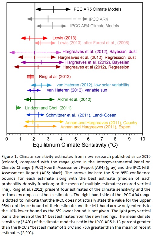
The determination of the global warming expected from a doubling of atmospheric carbon dioxide (CO2), called the climate sensitivity, is the most important parameter in climate science. The Intergovernmental Panel on Climate Change (IPCC) fifth assessment report (AR5) gives no best estimate for equilibrium climate sensitivity “because of a lack of agreement on values across assessed lines of evidence and studies.”
Studies published since 2010 indicates that equilibrium climate sensitivity is much less that the 3 °C estimated by the IPCC in its 4th assessment report. A chart here shows that the mean of the best estimates of 14 studies is 2 °C, but all except the lowest estimate implicitly assumes that the only climate forcings are those recognized by the IPCC. They assume the sun affects climate only by changes in the total solar irradiance (TSI). However, the IPCC AR5 Section7.4.6 says,
“Many studies have reported observations that link solar activity to particular aspects of the climate system. Various mechanisms have been proposed that could amplify relatively small variations in total solar irradiance, such as changes in stratospheric and tropospheric circulation induced by changes in the spectral solar irradiance or an effect of the flux of cosmic rays on clouds.”
Many studies have shown that the sun affects climate by some mechanism other than the direct effects of changing TSI, but it is not possible to directly quantify these indirect solar effects. All the studies of climate sensitivity that rely on estimates of climate forcings which exclude indirect solar forcings are invalid.
Fortunately, we can calculate climate sensitivity without an estimate of total forcings by directly measuring the changes to the greenhouse effect.
The greenhouse effect (GHE) is the difference in temperature between the earth’s surface and the effective radiating temperature of the earth at the top of the atmosphere as seen from space. This temperature difference is generally given as 33 °C, where the top-of-atmosphere global average temperature is about -18 °C and global average surface temperature is about 15 °C. We can estimate climate sensitivity by comparing the changes in the GHE to the changes in the CO2 concentrations.
The Clouds and Earth’s Radiant Energy System (CERES) experiment started collecting high quality top-of-atmosphere outgoing longwave radiation (OLR) data in March 2000. The last data available is June 2013 as of this writing on January 14, 2013. Figure 1 shows a typical CERES satellite.

Figure 1. CERES Satellite
The CERES OLR data presented by latitude versus time is shown in Figure 2.

Figure 2. CERES Outgoing Longwave Radiation, latitude versus date.
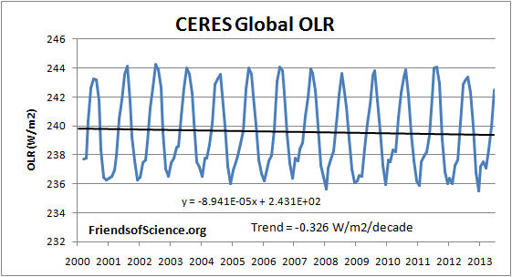
The global average OLR is shown in Figure 3.

Figure 3. CERES global OLR.
The CERES OLR data is converted to the effective radiating temperature (Te) using the Stefan-Boltzmann equation.
Te = (OLR/σ)0.25 – 273.15. where σ = 5.67 E-8 W/(m2K4), Te is in °C.
The monthly anomalies of the Te were calculated so that the annual cycle would not affect the trend.
We use the HadCRUT temperature anomaly indexes to represent the earth’s surface temperature (Ts). The HadCRUT3 temperature index shows a cooling trend of -0.002 °C/decade, and the HadCRUT4 temperature index shows a warming trend of 0.031 °C/decade during the period with CERES data, March 2000 to June 2013. The land measurement likely includes a warming bias due to uncorrected urban warming. The hadCRUT4 dataset added more coverage in the far north, where there has been the most warming, but failed to add coverage in the far south, where there has been recent cooling, thereby introducing a warming bias. We present results using both datasets.
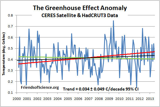
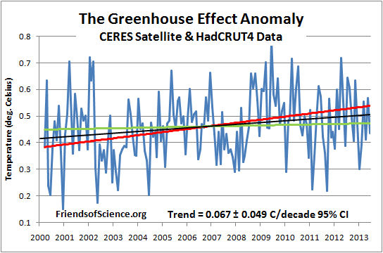
The difference between the surface temperatures anomaly and effective radiating temperature anomaly is the GHE anomaly. Figures 4 and 5 show the Greenhouse effect anomaly utilizing the HadCRUT3 and HadCRUT4 temperature indexes, respectively.

Figure 4. The greenhouse effect anomaly based on CERES OLR and HadCRUT3.

Figure 5. The greenhouse effect anomaly based on CERES OLR and HadCRUT4.
The trends of the GHE are 0.0343 °C/decade based on HadCRUT3, and 0.0672 °C/decade based on HadCRUT4.
We want to compare these trends in the GHE to changes in CO2 to determine the climate sensitivity. Only changes in anthropogenic greenhouse gases can cause a significant change in the greenhouse effect. Changes in the sun’s TSI, aerosols, ocean circulation changes and urban heating can’t change the GHE. Changes in cloudiness could change the GHE, but data from the International Satellite Cloud Climatology Project shows that the average total cloud cover during the period March 2000 to December 2009 changed very little. Therefore, we can assume that the measured change in the GHE is due to anthropogenic greenhouse gas emissions, which is dominated by CO2.
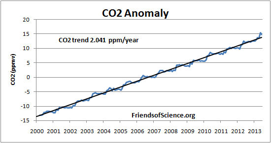
The CO2 data also has a large annual cycle, so the anomaly is used. Figure 6 shows the monthly CO2 anomaly calculated from the Mauna Loa data and the best fit straight line.

Figure 6. CO2 anomaly.
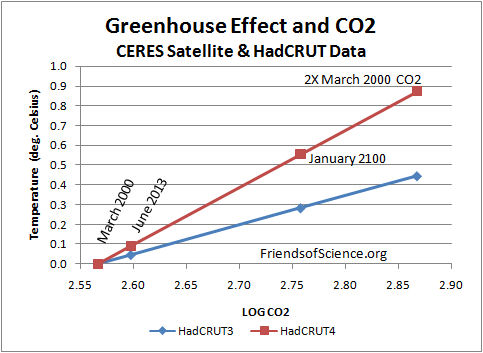
The March 2000 CO2 concentration is assumed to be the 13 month centered average CO2 concentration at March 2000, and the June 2013 value is that value plus the anomaly change from the fitted linear line. Table 1 below shows the CO2 concentrations, the logarithm of the CO2 concentration, and the change in the GHE from March 2000 for both the HadCRUT3 and HadCRUT4 cases.
Table 1 shows that the GHE has increased by 0.046 °C from March 2000 to June 2013 based on changes in the CERES OLR data and HadCRUT3 temperature data. Extrapolating to January 2100, the GHE increase to 0.28 °C by January 2100. Using the HadCRUT4 temperature data, the GHE increases by 0.55 °C by January 2100 compared to March 2000.
| hadCRUT3 | hadCRUT4 | |||
| Date | CO2 | Log CO2 | ΔGHE | ΔGHE |
| ppm | °C | °C | ||
| March 2000 | 368.88 | 2.567 | 0 | 0 |
| June 2013 | 395.94 | 2.598 | 0.046 | 0.089 |
| January 2100 | 572.68 | 2.758 | 0.283 | 0.554 |
| 2X CO2 | 737.76 | 2.868 | 0.446 | 0.873 |
Table 1. Extrapolated changes to the greenhouse effect (GHE) based on two versions of the hadCRUT datasets.
Table 1 shows that the GHE has increased by 0.046 °C from March 2000 to June 2013 based on changes in the CERES OLR data and HadCRUT3 temperature data. Extrapolating to January 2100, the GHE increase to 0.28 °C by January 2100. Using the HadCRUT4 temperature data, the GHE increases by 0.55 °C by January 2100 compared to March 2000.
The last row of Table 1 shows the transient climate response (TCR), which is the temperature response to CO2 emissions from March 2000 levels to the time when CO2 concentrations have doubled. TCR is less than the equilibrium climate sensitivity because the oceans have not reached temperature equilibrium at the time of CO2 doubling. TCR is calculated by the equation:
TCR = F2x dT/dF ; where dT means the temperature difference, dF means the forcing difference, from March 2000 to June 2013.
The CO2 forcing was calculated as 5.35 x ln (CO2/CO2i). The change in forcing from March 2000 to June 2013 is 0.379 W/m2. The forcing for double CO2 (F2x) is 3.708 W/m2. The TCR is 0.45 °C using hadCRUT3, and 0.87 °C using hadCRTU4 data. These values are much less than the multi-model mean estimate of 1.8 °C for TCR given in Table 9.5 of the AR5. The climate model results do not agree with the satellite and surface data and should not be used to set public policies.
Figure 7 shows the results of Table 1 graphically.

Figure 7. The greenhouse effect and CO2 extrapolated to January 2100 and double CO2 bases on CERES and HadCRUT data.
This analysis suggests that the temperature change from June 2013 to January 2100 due to increasing CO2 would be 0.24 °C (from HadCRUT3) or 0.46 °C (from HadCRUT4), assuming the CO2 continues to increase along the recent linear trend.
An Excel spreadsheet with the data, calculations and graphs is here.
HadCRUT3 data is here.
HadCRUT4 data is here.
Mauna Loa CO2 data is here.
CERES OLR data is here.
Total cloud cover data is here.
A linear trend? Based on a 13-year period? In other words, projected far enough into the future, we will burn? This assumes everything remains constant, of course. As if nature is static and the climate never changes.
The 33 K GHE claim, originally from 1981_Hansen_etal.pdf (Google it) is baseless. This is because Hansen et al asserted with absolutely no evidence that the -18 deg C temperature for the radiative emitter in equilibrium with Space is a zone in the upper atmosphere.
This is not true: it is the flux-weighted average temperature of three main emitting zones; the surface at 15 deg C via the ‘atmospheric window’, the lower troposphere for H2O bands and -50 deg C for the CO2 15 micron band in the owed stratosphere.
The real GHE according to the same flat SW absorber/spherical LW emitter model is ~11 K. Hansen et al ‘forgot’ that if you remove GHGs from the atmosphere, no clouds or ice, SW increases by 43%.
So, there is no 3x positive feedback. In reality the atmosphere self-controls by changing OLR nature to compensate for pCO2 change, also net insolation change as cloud area and albedo vary.
Furthermore, no professional scientist or Engineer can accept that the Earth’s surface emits net IR energy at the black body level. Unfortunately, Meteorology and Climate Alchemy teach incorrect physics, including that a pyrgeometer outputs a real energy flux when it is the Radiation Field, a potential flux to a sink at 0 deg. C: only the difference of RFs transfers energy.
Also the sign of the effect of aerosols on cloud albedo is wrong – this is because Sagan’s aerosol optical physics failed to consider a second optical effect, easily proved experimentally by the ‘Glory’ phenomenon.
Therefore, Climate Science needs to be restarted under new management with no investment in incorrect science so as to correct these major errors (there are many more including failure in interpret Tyndall’s Experiment – there can be no gas phase thermalisation of absorbed IR energy).
Only then can the excellent experimentalists such as those operating CERES get the correct platform to present their data, instead of being under essentially political control.
For comparison has anybody done RSS and UAH?
@ Katherine, that’s linear trend in CO2 increase, so yes liner trend is correct.
Any chance of an essay expanding on and consolidating all @AlecM’s points? That would be really useful!
@Peter Ward: in the mill. Climate Alchemy has been on the wrong track since Carl Sagan made 3 major physics’ mistakes leading him to conclude, wrongly, that GHGs cause Lapse Rate warming (it’s actually gravity).
I see even now Physicists assume the atmosphere is a grey-body emitter/absorber of IR energy – it’s really semi-transparent which is why OLR has been badly misinterpreted.
Katherine says: January 16, 2014 at 12:28 am
The dataset is short, so the extrapolation is uncertain, but it is the best dataset we have. The calculated transient climate response is the estimated effect of increasing greenhouse gases only. The small warming effect of CO2 can be easily be offset by natural climate change. We believe that the sun is a major driver of climate changes based on long-term correlations between solar activity and temperatures, so yes, temperatures might not increase for many years if solar activity remains low. The advantage of this direct calculation of changes in the greenhouse effect over the CERES era is that we do not need knowledge of total forcings or feedbacks.
garymount says: January 16, 2014 at 12:49 am
@ Katherine, that’s linear trend in CO2 increase, so yes liner trend is correct.
_______________________________
But isn’t CO2’s absorption of LW inversely logarithmic, did I hear? i.e.: its ability to absorb maxes out at 500 ppm or something? I would be grateful for clarification on that.
But if so, then the absorption is not linear, even if the increase in concentration is.
Purely gravitational lapse rates are refuted by this essay. If the lapse rate were due to gravity, it would be possible to create a perpetual motion machine powered by said gravity.
http://wattsupwiththat.com/2012/01/24/refutation-of-stable-thermal-equilibrium-lapse-rates/
AlecM says: January 16, 2014 at 12:43 am
Silver Ralph says: January 16, 2014 at 1:38 am
Yes, the CO2 absorption of LW is logarithmic. That means it does NOT max out at 500 ppm.
See Figure 7. It is a graph of temperature versus the LOG of CO2 concentrations.
you cannot estimate radiative feedbacks (climate sensitivity) without knowing the radiative forcing(s), both natural and manmade. Forcings and feedbacks are intermingled in unknown proportions, and CERES measures the sum of both.
AlecM says: January 16, 2014 at 1:11 am
There must be some GHGs for there to be a lapse rate, ie, a decline of temperature with altitude to the tropopause. The value of the lapse rate does depend on gravity, which is not changing. An increase in GHG would cause the height of the tropopause to increase. Some data suggests that water vapor in the upper troposphere and lower stratosphere declines with increasing CO2, partially offsetting the CO2 direct effect, resulting in the low transient climate response I have calculated.
Climate models do not assume the atmosphere is a greybody. They are based on line-by-line code calculations that correctly simulates a semi-transparent atmosphere, ie, with an atmospheric window. But the climate models apparently greatly overestimates positive feedbacks from clouds and water vapor.
@Ken Gregory: “If there were no greenhouse gases in the atmosphere, but the same albedo, the surface would emit the 240 W/m2, and the average surface temperature would be about -18 C.”
Correct but very misleading, I wonder why?
If there were no greenhouse gases in the atmosphere, there would be no clouds or ice hence the SW thermalised at the surface would by definition be up to 43% higher. That would make the average surface radiative equilibrium temperature with Space of the flat SW absorber/spherical LW emitter 4 to 5 deg. C, a GHE of ~11 K. Thus the 3x ‘positive feedback’ is imaginary, a result of a rash assumption not picked up by peer review in 1981 and on which all the predictions of catastrophic warming are based.
Thus, to achieve 33 K GHE in the climate modelling, IR absorption in the atmosphere is increased over reality by a factor of 157.5/23 = 6.85x. If necessary, I can describe to readers how this numerical prestidigitation works (it involves another bit of incorrect physics). The hypothetical evaporation of sunlit oceans rises, hence the ‘positive feedback’, but the average atmospheric temperature also increases.
In 2010, US cloud physicist G L Stephens remarked that this temperature increase is corrected in the climate models during hind-casting, with no publicity, by using double real low level cloud optical depth, about 25% albedo increase. Because of this, the IPCC climate models cannot predict climate. It’s time to stop this farrago.
I’ve got a number of problems with this essay, as have some others. The timescale is surely too short for drawing any conclusions, especially as those conclusions depend on linear extrapolation of the small difference between two larger values. The CO2 effect appears to be treated as global, while the IPCC report makes it clear that its effect is concentrated mainly in the tropical troposphere [AR4 fig 9.1]. The essay asserts that “Changes in the sun’s TSI, aerosols, ocean circulation changes and urban heating can’t change the GHE“, but can they affect these calcs?- eg. GHE is being estimated using measured OLR as one of the inputs, OLR includes reflected LR, so would change if TSI changed. Maybe the other factors have the potential to affect the result too?
If all of the above issues are able to be dismissed, then one way of testing would be to select some subsets of the data period and apply the same calcs to each. Variation between results could indicate that the results are not reliable.
Ken Gregory:
I like your results so I wish I could accept them, but I cannot.
You say
Yes, and you say of your analysis
This finding agrees with other direct analyses which suggest ~0.4°C global temperature rise for a doubling of atmospheric CO2; e.g.
Idso from surface measurements
http://www.warwickhughes.com/papers/Idso_CR_1998.pdf
and Lindzen & Choi from ERBE satellite data
http://www.drroyspencer.com/Lindzen-and-Choi-GRL-2009.pdf
and Gregory from balloon radiosonde data
http://www.friendsofscience.org/assets/documents/OLR&NGF_June2011.pdf
Hence, you can see why I like your results so I am tempted to accept your analysis, but the following explains why I do not accept it.
You say you analysed
And your error estimates for those trends are?
Please note that the trend values span zero.
You say
This implies that you think the difference between the trends of the data sets is a result of the methods used to compile the temperature data sets. And you strengthen this implication saying
Sorry, but I do not agree.
The trends are not statistically significant from zero at 95% confidence because of the variances of the data sets. Your analysed “trends” are provided by random noise in the data. For your results to be valid they should be obtained from the extreme values allowed by the confidence limits of the trend lines (at 95% confidence). This would increase the spread of indicated global temperature rise projections to January 2100 to be greater than the 0.24 °C to 0.46 °C.
A result which is compiled from the variance of its analysed data is not valid.
I think your analysis provides a correct conclusion but that conclusion is obtained by analysis of apparent trends which result from the inherent errors in the data set. If your trend values were the extreme values allowed by the confidence limits of the trend lines (at 95% confidence) then your result would be valid. So, if I were asked to peer review your paper as reported above then I would commend that it not be accepted for publication. Sorry.
Richard
Two mysteries:
1) If the CO2 increase is largely anthropogenic as claimed by the IPCC, why does Figure 6 show no evidence of the decrease in consumption in much of the world after the 2008 financial crisis?
2) Why does AlexM repeat the same claims on every thread that mentions the GHE despite being unable to convince anyone ever that he knows what he’s talking about?
Ken Gregory says:
January 16, 2014 at 1:37 am
The advantage of this direct calculation of changes in the greenhouse effect over the CERES era is that we do not need knowledge of total forcings or feedbacks.
Doesn’t this assume that changes in the unknown forcings will average out and remain constant? For example, if Svensmark’s cosmic ray theory is valid and there’s a spike in galactic cosmic rays, your direct calculation would require the various other forcings to adjust so that CO2’s effect dominates. But why should they?
Also, in your original post, you wrote, “Changes in cloudiness could change the GHE, but data from the International Satellite Cloud Climatology Project shows that the average total cloud cover during the period March 2000 to December 2009 changed very little. Therefore, we can assume that the measured change in the GHE is due to anthropogenic greenhouse gas emissions, which is dominated by CO2.” While the average total cloud cover may have changed very little, Willis’s posts have shown that where the clouds appear can have a marked difference in how much sunlight gets through to warm the Earth. A decrease in cloudiness over the tropics could be offset by cloudiness in the temperate or polar regions for a net change of zero to the average total cloud cover but an overall increase in energy input, so just because the average changed very little doesn’t mean clouds can be disregarded.
Ken Gregory says:
January 16, 2014 at 1:50 am
Figure 2 shows that CERES measures the outgoing longwave radiation (OLR) at 240 W/m2. We are not assuming that all of this originates from the atmosphere. Some is emitted directly from the surface through the atmospheric window. However, the 240 W/m2 observed from space corresponds to a blackbody temperature of -18.1 deg. Celsius. If there were no greenhouse gases in the atmosphere, but the same albedo, the surface would emit the 240 W/m2, and the average surface temperature would be about -18 C.
But if there were no greenhouse gases in the atmosphere, there wouldn’t be any water vapor and therefore no clouds. In which case, how could you expect to have the same albedo?
Ken,
You can only say that the average surface temperature is -18C if you assume the following;
1. The Earth is flat and not a sphere
2. There is no day/night cycle
3. The solar energy input is reduced by a factor of 4 from what it actually is at TOA.
Not a good basis to build any sort of analysis really …
There is no need of the GHE because the measured outgoing energy does not come from the surface but 5-6Km up in the atmosphere, ie., the cloud tops. Also the outgoing energy is from the whole planet surface but solar heating is on one hemisphere. This minor effect, the rotating planet with a day and night cycle, is ignored by the AR4 K&T energy balance graphic which assumed a flat non rotating earth. With reality in the equation the GHE is not necessary.( let alone the fact that it violates the laws of thermodynamics).
Dancing polar vortex and solar activity.
http://losyziemi.pl/niezwykly-taniec-wiru-polarnego-ktory-silnie-reaguje-na-aktywnosc-slonca#more-25893
Roy Spencer says: January 16, 2014 at 2:10 am
Roy, I am familiar with your work, and I am very aware that forcings and feedbacks are intermingled in unknown proportions. However, I am using CERES and HadCRUT to measure the change in the greenhouse effect. I make no estimate of total forcings or feedbacks.
I wrote, “The HadCRUT3 temperature index shows a cooling trend of -0.002 °C/decade, and the HadCRUT4 temperature index shows a warming trend of 0.031 °C/decade during the period with CERES data, March 2000 to June 2013.” Both are insignificant temperature trends, so there was no change in temperature, and there was no feedbacks during the period!
There may be natural and man-made forcings during the period such as ocean circulation changes and lower solar forcings, but these do not change the greenhouse effect, ie the difference between the surface temperature and the effective radiating temperature. If fact, there must be negative forcings during the period to cause the “pause” in global warming. Only changes in the greenhouse gases and clouds will change the greenhouse effect. The IPCC says cloud cover can change only by a temperature change, ie, a feedback, but there was no temperature change during the period. A change in cloud cover could potentially change the OLR, but the ISCCP data shows no significant change in total cloud cover during the period. I use changes in CO2 to represent all man-made GHGs.
The TCR = 3.71 W/m2 X (dT/dF), where the dT is the change in the greenhouse effect over the period, and dF is the corresponding change in greenhouse gas forcing over the period, which is the ONLY forcing that would cause the dT. TCR for the HadCRUT3 case is 0.45 C for double CO2.
@Ken Gregory: you are correct:; the radiation transfer modelling does not assume a grey body. Indeed, the RTM is about the only thing in Climate Alchemy I trust!
My comment about the grey body assumption is that it was used by Houghton, copying Sagan, to claim the GHE causes lapse rate warming. It doesn’t; gravity does. A recent paper from Brookhaven used a grey body assumption so this beast is still alive in atmospheric physics.
We now get to the ‘enhanced greenhouse effect’ and Sagan’s ‘Venusian thermal runaway’ transferred to the Earth. It came down to the idea that when temperature exceeds a critical level, water ceases to condense so pH2O increases at the same time as lapse rate nearly doubles.
The problem is that these calculations assume the planetary surface emits net IR energy at the black body level. No professional scientist or engineer can accept this. I have measured, experimentally, coupled convection and radiation in metallurgical plants, also in research. We invented GHG physics so know rather a lot about it.
Radiation fields interact vectorially so there can be no emission from equal temperature surface to atmosphere of IR energy in any self-absorbed GHG band. [There’s a new bit of physics here.] The concept of ‘forcing’ is plain wrong. Increased pGHG reduces net surface IR emission. In the absence of any other factor the surface temperature would increase, hence the 1.2 K CO2 climate sensitivity would be correct. However, other processes offset this temperature rise reducing real CO2 climate sensitivity; it’s probably <0.1K.
To summarise, in climate modelling the RTM works fine. However, the Big Mistake is to put in 333W/m^2 imaginary IR from the surface to the atmosphere, apparently offset by applying Kirchhoff's Law of Radiation at ToA. I have spoken to modellers attempting to justify this by crazy S-B calculations. They are absolutely wrong because 134.5 of the net 157.5 W/m^2 'Clear Sky Atmospheric Greenhouse Factor' is a perpetual motion machine of the 2nd kind, hence the need for arbitrary cooling in hind-casting, that cooling having been apparently hidden until 2010.
@Katherine
Katherine says: January 16, 2014 at 12:28 am
It is actually a logarithmic trend with CO2. So on that graph d(log(2C)) = DT(0.8) . So on that basis even if in the unlikely event that CO2 levels were to quadruple to 1100 ppm by say 2300 global temperatures would still only rise by 1.6C. That is assuming the analysis is correct.
@ Silver Ralph, I was talking of measured quantity, not its effect. It is my best guess that business as usual with emissions will be the best method of determining climate sensitivity to forcing in the shortest time possible. This would be the best policy for governments for the sake of the children ™.
@steveta_uk: “Why does AlexM repeat the same claims on every thread that mentions the GHE despite being unable to convince anyone ever that he knows what he’s talking about?”
Answer: because until somebody comes up with a scientific argument, backed up by experimental evidence, proving that I am wrong, it is my duty as a scientist to push the bloody point ad nauseum.
No-one has yet taken me on, probably because I am one of the very few still active who has made real measurements of coupled convection and radiation, and have along with very few others around the World set out to understand the real nature of radiative energy transfer.
I’ll give you an example. The Law of Conservation of Energy between the material and EM worlds is: qdot = -Div Fv where qdot is the monochromatic rate of heat generation per unit volume of matter and Fv is the monochromatic radiative flux density. All scientists and engineers i have talked to forget about the negative sign. Many otherwise competent physicists imagine matter fires out photons according to the S-B equation. This explains why Sagan and Houghton got it wrong.
It’s a Big Mess and until Climate Alchemy dumps the ‘back radiation’ and ‘forcing’ concepts, there can be no progress except phoney modelling to pretend the subject knows what it is doing. That does’t fool me and Nature is showing the reality, which is that the claimed CO2 climate sensitivity of the IPCC is a lavishly-funded confidence trick.
I hate and loath all use of ‘Linear Trends’, OLS or otherwise. They are only of use to infill values within the period they cover (at best). They are completely useless outside of the data range they are drawn from.
‘Linear Trends’ = ‘Tangent to the curve’ = ‘Flat Earthers’.
“‘Linear Trends’ = ‘Tangent to the curve’ = ‘Flat Earthers’.”
– – –
When you watch a movie or play a game console game that uses computer generated graphics, every pixel for the image is generated from straight lines. This also applies to Finite Element Analysis for engineering applications. Its really a matter of computer resources that determines the accuracy.
richardscourtney says: January 16, 2014 at 2:34 am
The temperature trend is near zero, but the trend in the greenhouse effect is significantly positive. You can judge the uncertainties in the estimates by observing how closely the greenhouse effect curves follow the best fit line. The R2 value for the fit in Figure 4 for HadCrut3 is R2 = 0.012. The difference in the TCR results between HadCRUT3 and HadCRUT4, 0.45 C and 0.87 C, respectively, further shows that the TCR is uncertain. The data is messy, that that is the best we have.
This calculation does not require direct knowledge of the total forcings operating in the climate system. The forcing from indirect solar effects are unknown, but they must be substantial because there are strong correlations between solar activity and global temperatures. Any method to estimate climate sensitivity that requires an estimate of total forcing but only uses the IPCC recognized forcings are totally useless because they ignore indirect solar forcings.
You provided a link to my article “Out-going Longwave Radiation and the Greenhouse Effect” which estimates climate sensitivity at 0.4 C. That paper used a long dataset from 1960, and used radiosonde humidity data to calculate OLR, which is uncertain, but the general method is the same. This article uses a short, but high quality CERES dataset, and also gets low climate sensitivity.
@ RichardLH , Upon a second reading of your statement, “They are completely useless outside of the data range they are drawn from” is something I agree with somewhat. A trend line is different than a trend but unfortunately the general public are not versed in these nuances, as I was not 4 years ago either. (Thanks WUWT and W. M. Briggs amongst others for the education).
The blackbody radiation equates to a surface temperature of -18 degrees.
Why should we assume that the “surface” as seen by an instrument in space is ground level and not some altitude within our atmosphere? How is the lapse rate accommodated by GHG theory or is it ignored?
AlecM said:
“Answer: because until somebody comes up with a scientific argument, backed up by experimental evidence, proving that I am wrong, it is my duty as a scientist to push the bloody point ad nauseum.”
That’s how I feel, too 🙂
We still have people saying no lapse rate without GHGs when there obviously would be a lapse rate due to decreasing density with height and uneven surface heating leading to density variations with lighter air parcels rising above heavier parcels which is all that convection is.
garymount says:
January 16, 2014 at 3:56 am
It is just a nice ‘trick’ to be able to use the ‘flat earthers’ gibe in reverse sometimes, usually against CAGW.
‘Linear trends’ are not trends, they are lines drawn on a range of data, useless outside of the data range they are drawn on.
An elegant analysis.
In 2007 Stephen Schwartz of the Brookhaven Lab did a study base on ocean heat content and came up with 1.1 ± 0.5 K. Heat capacity, time constant, and sensitivity of Earth’s climate system. Schwartz S. E. J. Geophys. Res., 112, D24S05 (2007). doi:10.1029/2007JD008746
Given Schwartz’s wide error bars his lower would be 0.6 and upper 1.7 K.
The average of your figures of 0.45 °C and 0.87 °C is,0.66 K and that figure is within the range estimated by Schwartz..
Since the two methodologies are completely unconnected this is an impressive effort on your part. Why not publish?.
AlecM says:
January 16, 2014 at 3:17 am
Right on Alec.
You do not have to convince me.
@steveta_uk ; you are going to have do your homework before making untrue comments.
He should also read this post………
“johnmarshall says:
January 16, 2014 at 2:54 am ”
@steveta_uk ; try this:
http://greenhouse.geologist-1011.net/
1) If the CO2 increase is largely anthropogenic as claimed by the IPCC, why does Figure 6 show no evidence of the decrease in consumption in much of the world after the 2008 financial crisis?
Global CO2 emission in Gt/a (BP Statistical Review 2013)
2004….28.603
2005….29.453
2006….30.320
2007….31.197
2008….31.540
2009….31.100
2010….32.840
2011….33.743
2012….34.466
The change is not large enough to show clearly in the atmospheric total CO2 – especially when there are other sources and sinks to be accounted for.
A trend is a trend is a trend
But the question is, will it bend?
Will it alter its course
Through some unforeseen force
And come to a premature end?
Sir Alec Cairncross, economist.
Schrodinger’s Cat says:
January 16, 2014 at 4:02 am
We don’t assume that. We are able to determine the temperature of planets and stars by observing the spectrum of radiation that they produce. This has been possible for over 100 years.
Seen from space, we would assess the temperature of the earth to be 255K. Even before the satellite era, it was possible to make some assessment by estimating the solar radiation reaching the earth, on the basis that of what comes in equals what goes out (conservation of energy). I believe Brian Cox performed such a TV experiment by warming a pan of water under full sun and estimating the watts required for such heating.
So, in summary, we see the temperature of the earth from space as being 255K, but we know by living here that the SURFACE of the earth is much hotter than that. So how is the discrepancy explained? That is where the GHE comes in, and it is excellently explained in an earlier WUWT post this month http://wattsupwiththat.com/2014/01/12/global-warming-is-real-but-not-a-big-deal-2/
Even before Arrihenius’s paper of 1896 it was realised that “the temperature of the earth would probably fall to -200 degC if the atmosphere did not possess the quality of selective absorption” (a figure we now know to be much too low).
The greenhouse effect was a topic of study in our 1970 theoretical geophysics course. At that time the greenhouse effect was a theoretical metric for comparing the atmospheric insulation of the planets. we did this using the solar constant of 1367W/m^2 (and an appropriate increase for Venus which is closer and for Mars which is further). We used 0.3 for the Earth’s albedo and assumed a surface temperature of 288 k (approximately 15°C). This gave us 255 k for the effective radiative temperature which subtracted from the 288 k surface temperature gave us 33°C for the greenhouse effect.
Ken’s calculation of the greenhouse effect based on CERES OLR data covers the period since 2000 during which there was net global cooling. This exposes the fallacy of AGW in two ways.
First of all the CERES OLR data shows a net decrease in OLR with cooling temperatures. For this to occur there has to be a net decrease in incoming energy and since this change is not visible in the TSI measurement the only source for this decrease in incoming energy is increased albedo from a net increase in cloud cover.
The second and more critical aspect to the issue of AGW is that the greenhouse effect is increasing as the temperature is decreasing which is contrary to the AGW conjecture which would require a decrease in greenhouse effect with decreasing temperature for the AGW hypothesis to be valid and this is simply not the case.
Since the issue here is global warming and there has been a net 0.4°C of global warming since 1980 (ending by 1997), to see how this relates to global warming we need to look at OLR data covering the period when warming occurred. Fortunately this data was recorded by weather satellites since their launch in late 1978 and a graph of this OLR data is nicely presented on the Climate for You website (www.climate4you.com) compiled from data available from NOAA at http://www.esrl.noaa.gov/psd/data/gridded/data.interp_OLR.html
This dataset is clearly not as accurate as the CERES data showing OLR to be on average 232W/m^2 compared to the 239W/m^2 shown on the CERES data, but it does go back to when the global temperature was increasing and can provide the basis for a calculation of the greenhouse effect over the period from 1980 to 2010.
When calculated for these two years the greenhouse effect actually decreased from 35.56°C in 1980 to 35.42°C in 2010 demonstrating that the 70.9% increase in CO2 emissions since 1980 never actually enhanced the greenhouse effect and therefore completely refuting the basis for AGW conjecture.
Ken’s demonstration using CERES OLR data shows an increase in greenhouse effect with decreasing global temperature and my demonstration using OLR data from weather satellites shows decreasing greenhouse effect with increasing global temperature. Either of these demonstrations proves that changes to incoming energy from changes in albedo and definitely not CO2 is driving the changes in global temperature and combined these demonstrations make the proof incontrovertible. This change in albedo is demonstrated by Project Earthshine which shows the albedo decreasing to 1998 and then increasing since.
A change in albedo resulting from changes in cloud cover fits very nicely with Svensmark’s hypothesis of solar activity controlled cosmic ray cloud nucleation giving us both confirmation of solar theory for global temperature change and incontrovertible evidence that the AGW hypothesis is pure bunk.
“Only changes in anthropogenic greenhouse gases can cause a significant change in the greenhouse effect. ”
I don’t understand why you believe this base assumption to be axiomatic. Doesn’t it imply that all natural sources of CO2 are constant?
I think you could only do this if you had data extending beyond known cycles (60-80 years to cover a complete PDO, AMO etc…). Because of where we are in the PDO cycle with this data, I would have to assume your result estimates the lower bound rather than the center.
Ken Gregory:
Thankyou for your post at January 16, 2014 at 3:44 am
http://wattsupwiththat.com/2014/01/16/ceres-satellite-data-and-climate-sensitivity/#comment-1537703
in reply to my post at January 16, 2014 at 2:34 am
http://wattsupwiththat.com/2014/01/16/ceres-satellite-data-and-climate-sensitivity/#comment-1537664
Obviously, I was not clear because your reply does not answer my point. I will try to do better this time.
I wrote
I bolded that to ensure it would not be missed so it must be that it is not sufficiently clear.
Your results are obtained from the AVERAGE trend of each time series you analysed. But the data are noisy and – as you agree – the average trend is near zero in each case. Indeed, as I said, the difference between the trends of the two data sets spans zero.
Your obtained range of results is not valid because you have adopted unjustifiable trend values.
For example, you could have used zero trend and obtained a single and different result. But you used the average trend of each data set to provide a single result from each of the two data sets then quoted the obtained results to provide a range; i.e. between 0.24 °C to 0.46 °C for projected indicated global temperature rise projections to January 2100.
Each data set provides a range of possible trend values to within specified confidence (climate science uses 95% confidence). Hence, there is a maximum trend and a minimum trend at 95% confidence for EACH of your two analysed time series. Using these values would provide A RANGE OF PROJECTIONS FOR EACH DATA SET to within 95% confidence.
A combination of the two analyses would then obtain a wide range from the lowest of the two minimum projections to the highest of the two maximum projections and would be to 95% confidence.
In conclusion, using the average trend of each data set provides results which are induced by the variances of the data sets. In other words, your results are solely a result of ‘noise’ in the data. But, as I have explained, you could re-do the analysis to provide valid results with stated confidence.
Richard
The moon has a Bond albedo of 0.11, and a SB theoretical temperature of 270.7K according to NASA:
http://nssdc.gsfc.nasa.gov/planetary/factsheet/moonfact.html
Yet the average temperature at the equator (the hottest latitude) is just 206K according to NASA using its Diviner measurements:
http://diviner.ucla.edu/science.shtml
There is no significant atmosphere, but a large divergence between supposed theory and actual measurement.
Eric Worrall says:
January 16, 2014 at 1:46 am
Purely gravitational lapse rates are refuted by this essay.
http://wattsupwiththat.com/2012/01/24/refutation-of-stable-thermal-equilibrium-lapse-rates/
==========
I reread Dr Brown’s essay. From what I read he is not attributing the lapse rate to GHG. Rather to rising and falling parcels of air due to heating and cooling of the surface. These rising and falling parcels of air would still exist in the absence of GHG due to the rotation of the earth and seasonal differences, thus the lapse rate cannot be a product of GHG.
This is further confirmed by the dry air lapse rate 9.8C/km being equivalent to gravitational acceleration 9.8 m/s2.
It seems clear that the DALR is a result of conversion of PE to/from KE, and the energy to drive the system comes primarily from heating of the surface, either by the sun or the earth’s core. Without this heating the atmosphere would be isothermal, regardless of GHG.
So from this it would seems that gravity and surface warming/cooling determine the lapse rate, not GHG.
thinking more on the DALR, since GHG absorbs/radiates energy, adding it to the atmosphere could also provide a heating/cooling effect on the atmosphere, which would also lead to rising and falling parcels of air as per Dr Brown’s essay, so GHG could also contribute to the lapse rate along with surface heating and cooling.
“The difference between the surface temperatures anomaly and effective radiating temperature anomaly is the GHE anomaly.”
Could you expand on that a bit? The surface-temperature anomaly comes from the average of the local temperatures, not the fourth root of the average of the temperatures’ fourth powers. Even though the surface-temperature anomaly stays constant, the extremes could moderate, and that would reduce the average Stefan-Boltzmann radiation.
You may have checked that this effect is negligible here, but your post doesn’t say so.
There is a cyclic variation in OLR of about 8W/m^2 over the course of a year due to changes in albedo from the snow cover in the larger northern hemisphere temperate landmass. That being said the average OLR over the course of a year must by energy balance equal the average net incoming energy minus that portion of the energy permanently incorporated into the Earth system through such processes as plant growth and ocean warming.
If over a ten year period OLR decreases, temperature decreases and the greenhouse effect increases the trend is long enough for an incontrovertible conclusion that the increase in atmospheric CO2 concentration over the last decade did not cause global warming through enhancement of the greenhouse effect.
Similarly over the period of the last 33 years there has been a net increase in OLR a net increase in global temperature but a net decrease in the greenhouse effect. This means that the increase in atmospheric CO2 concentration did not enhance the greenhouse effect causing the observed 0.4°C of net warming since 1980.
We do not need trends any longer than either of these to confirm that CO2 is not driving global temperature in the way predicted by the IPCC climate models explaining why they have all been wrong predicting warming when the Earth has been cooling since 2002
Eric Worrall says:
January 16, 2014 at 1:46 am
Purely gravitational lapse rates are refuted by this essay. If the lapse rate were due to gravity, it would be possible to create a perpetual motion machine powered by said gravity.
http://wattsupwiththat.com/2012/01/24/refutation-of-stable-thermal-equilibrium-lapse-rates/
Eric, I am surprised that you did not see the logical error in his Brown’s argument. He described a situation in which the top and bottom of a thermally isolated container of gas was connect via separate and thermally isolated silver wire. Separation of the wire from the gas container was not significant to his argument as the same results would occur with the wire simply running vertical within the gas container. In both cases, the addition of the silver wire produces a new system with the adiabatic lapse rate dominated by the most thermally conductive component, the wire. It is the characteristics of the total system that determine the final results. A tube of isolated gas and a similar tube with a thermal conductor inserted are qualitatively and quantitatively different and cannot be used to refute static adiabatic lapse rate. While his conclusion may in fact be correct, his thought experiment did not prove it.
Mike Jonas says: January 16, 2014 at 2:29 am
In the equation TCR = F2x dT/dF, the dT is the temperature change of the greenhouse effect, it is NOT the surface temperature change nor the top-of-atmosphere effective radiating temperature alone. A change of TSI it would change both the surface temperature (Ts) and the effective radiating temperature (Te) equally, so there would be no change in the GHE, which is Ts – Te. The GHE will change only if the longwave absorption in the atmosphere changes, resulting in a change in the downward longwave radiation. Changes in TSI, aerosols, PDO, and albedo do not change LW absorption. The dF is the forcing that caused the change in dT, which is ONLY the change in greenhouse gases during the period.
You’re attempting to estimate the long-wave component of sensitivity but not saying anything about any possible short-wave component, right?
The way you see it, that is, OLR for a given (appropriately determined) surface temperature tells us how “hard” (1) invisible greenhouse gases and (2) visible clouds make it for the warm surface to radiate out into space, but it doesn’t say anything about how much clouds and snow in some way caused or suppressed by those gases reflect short-wave radiation back out.
In other words you aren’t attempting to capture any extent to which cloud and snow reflection of short-wave radiation respond to CO2 concentration and thereby contribute to sensitivity?
Bill Marsh says: January 16, 2014 at 5:29 am
It implies that natural sources of CO2, averaged over the annual cycle, does not change other than any feedback temperature response. There is an obvious annual cycle of natural CO2 production and absorption. I used the CO2 anomaly to calculate the CO2 trend so the annual cycle doesn’t affect the trend. There was no temperature change during the CERES period, so there was no feedback response of natural CO2 production. If volcanoes increased emissions, sure, that would affect the trend, but there have been no major volcanic eruption during the period, and volcanic CO2 is very small compared to human sources.
Ken
A change of TSI it would change both the surface temperature (Ts) and the effective radiating temperature (Te) equally
Don’t think so. Ts would rise faster than Te, even with constant GHE.
Norm Kalmanovitch says: January 16, 2014 at 5:18 am
Hmmm says: January 16, 2014 at 5:36 am
My calculations are based on changes in the GHE. How do the think PDO and AMO affects longwave absorption, downward longwave radiation, or the Ts-Te difference? They can’t. PDO and AMO affects surface temperatures Ts, but do not change the GHE.
MikeB says: “I believe Brian Cox performed such a TV experiment by warming a pan of water under full sun and estimating the watts required for such heating.”
You are correct he did such a experiment in Death Valley I believe and demonstrated that some 1000 W/m^2 was raining down on the earth at that location. Tough to get 255 K out of 1000 W/m^2.
Not on subject but: Per the EIA (Energy Info Agency) the 2nd week of Jan. Natural Gas net draw from storage was 287 Billion cu. ft. This is a record draw for any week of the heating season for the past 21 seasons. The second highest record 285 B cu ft was the second week of Dec 2013 also this season. The previous record draw was 266 billion cu ft the 2nd week of Jan 2010. Any time the draw exceeds 200 B Cu Ft It usually correlates with a negative temperature anomaly in the US for that week.
The following link provides access to a XL storage history spread sheet link.
http://ir.eia.gov/ngs/ngs.html
richardscourtney says: January 16, 2014 at 5:44 am
Richard, I agree with everything you said here, and for a technical journal submission, a statistical analysis with 95% confidence intervals would be necessary. A 95% confidence range of possible values for TCR would be significantly wider than the two values I presented. The uncertainties are much more than just the random noise. We don’t know what systematic errors are in the surface and satellite measurements, so even a 95% confidence interval will not give the full range of possible values. It is clear that the values presented are just the best estimates based on the two datasets used. That is fine for a blog post.
Eric Worrall says:
January 16, 2014 at 1:46 am
Purely gravitational lapse rates are refuted by this essay. If the lapse rate were due to gravity, it would be possible to create a perpetual motion machine powered by said gravity.
http://wattsupwiththat.com/2012/01/24/refutation-of-stable-thermal-equilibrium-lapse-rates/
====================================================================
The problem with the supposed proof is that it uses an unmodified version of Fourier’s Law. If there is an exchange of kinetic and gravitational potential energy in the gas column, then there must also be a similar exchange that goes on in the silver wire.
I really don’t understand all the resistance to this idea. It’s as if proof of the existence of atoms is still in doubt.
If one believes in atoms, then one must accept that as they move through a gravitational field that there will be an exchange of kinetic energy and gravitational potential energy. Collisions don’t change this.
Joe Born says: January 16, 2014 at 7:29 am
Willis Eschenbach had commented on this point a few times. The 4th root of the average surface radiation flux is not quite equal to the average of the 4th root of the surface radiation fluxes. Over the range of temperatures we are dealing with, the error is small. I don’t think this is relevant to my post because the the earth’s temperature range over the surface area has not likely changed over the 13 year period, so it wouldn’t affect the trends.
The surface of the Earth with no atmosphere would be the same as the moon, which is at 127 deg C in sunlight (-173 deg C on the dark side).
As climate models assume 24 hour a day sunlight, the 127 deg C temperature is applicable.
So, without an atmosphere, the Earth would be at 127 deg C at the surface and, instead, with an atmosphere is at 15 deg C. It is not a big stretch to see that the atmosphere clearly cools the planet’s surface, giving the surface more ways to shed heat, by conduction and convection, rather than just by radiation with no atmosphere.
As the temperature of the upper atmosphere varies with altitude quite radically, it makes no sense to pretend that there is a greenhouse effect that does not resemble a greenhouse at all and whose conditions are essentially arbitrarily chosen.
It doesn’t add up… says:
January 16, 2014 at 7:11 am
The moon has a Bond albedo of 0.11, and a SB theoretical temperature of 270.7K according to NASA:
http://nssdc.gsfc.nasa.gov/planetary/factsheet/moonfact.html
Yet the average temperature at the equator (the hottest latitude) is just 206K according to NASA using its Diviner measurements:
http://diviner.ucla.edu/science.shtml
There is no significant atmosphere, but a large divergence between supposed theory and actual measurement.
The lunar surface absorbs some energy and re-emits it, but it also reflects some without absorption. Presumably then the surface heating is less than total incoming energy. Presumably at least some of the difference can be accounted for by that.
“Changes in the sun’s TSI, aerosols, ocean circulation changes and urban heating can’t change the GHE.”
But increased NPP can account for at least a portion of reduced outgoing LWR.
What,for goodness sake is going on here !. Barely four days after this site invited a guest to write an article that included this –
‘GLOBAL WARMING IS REAL’
“Yes, the world has warmed 1°F to 1.5°F (0.6°C to 0.8°C) since 1880 when relatively good thermometers became available. Yes, part of that warming is due to human activities, mainly burning unprecedented quantities of fossil fuels that continue to drive an increase in carbon dioxide (CO2) levels. The Atmospheric “Greenhouse” Effect is a scientific fact!”
Damnest thing I have seen in over two decades on the forums
‘Any chance of an essay expanding on and consolidating all @AlecM’s points? That would be really useful!”
Yes, submit them to the nobel prize committee. Were he correct he would surely win the prize.
It bears repeating
‘Roy Spencer says:
January 16, 2014 at 2:10 am
you cannot estimate radiative feedbacks (climate sensitivity) without knowing the radiative forcing(s), both natural and manmade. Forcings and feedbacks are intermingled in unknown proportions, and CERES measures the sum of both.”
“higley7 says:
January 16, 2014 at 9:51 am
The surface of the Earth with no atmosphere would be the same as thhe moon, which is at 127 deg C in sunlight (-173 deg C on the dark side).
As climate models assume 24 hour a day sunlight, the 127 deg C temperature is applicable.”
######################
WRONG. yes virginia climate models have day and night. That is how, for example, we compare the diurnal range between models and observations.
knowledge is limited but stupidity is unbounded
Eric Worrall:”Purely gravitational lapse rates are refuted by this essay. If the lapse rate were due to gravity, it would be possible to create a perpetual motion machine powered by said gravity.”
Scot: “The problem with the supposed proof is that it uses an unmodified version of Fourier’s Law. If there is an exchange of kinetic and gravitational potential energy in the gas column, then there must also be a similar exchange that goes on in the silver wire.”
For the reasons I gave on that thread, I agree that Dr. Brown’s “refutation” left something to be desired. But, although as I read them the papers cited on that thread dictate an equilibrium kinetic-energy gradient, the gradient they specify is as a practical matter too small to be measured. Indeed, it may be too small to be measured even in principle. For all practical purposes, that is, the temperature in a gravitational field would be uniform at equilibrium.
But differential surface heating and conduction from the surface to the atmosphere would still happen even if the atmosphere were perfectly transparent, so equilibrium still wouldn’t prevail. Whether the resultant disturbances would result in much of a lapse rate is another question, though.
Joe Born says: January 16, 2014 at 8:17 am
Climate sensitivity to CO2 is the ratio of the surface temperature change that was caused by CO2 increases, including any feedbacks, to the change in CO2 forcing that caused that temperature change. But we don’t know directly what part of the surface temperature change was caused by the CO2 change. The greenhouse effect is the difference between the surface temperatures and the top-of-atmosphere temperatures, determined by OLR. OLR can change over the short term for many reasons not related to CO2. But the GHE changes primarily by changes in greenhouse gases, which affect the longwave radiation, not shortwave. Changes is albedo from changes in “cloud and snow reflection of short-wave radiation” will change surface temperatures and will change OLR, but will not change the GHE, which depends on longwave absorption and the resulting back radiation. That is, albedo changes Ts and Te equally, so no change in Ts – Te = GHE. So no, we don’t need to know the changes in short-wave radiation to calculate climate sensitivity.
AlecM 3:17am: “The Law of Conservation of Energy between the material and EM worlds is: qdot = -Div Fv where qdot is the monochromatic rate of heat generation per unit volume of matter and Fv is the monochromatic radiative flux density…I …made real measurements “
Cite? I am interested to read up on your publications or those of others that are similar, thx. The top post discussion of forcings, GHE and atm. fluid SW/OLR energy conservation seems complete enough without need of applying this formula.
One of the few others you claim exist “..around the World set out to understand the real nature of radiative energy transfer” published Radiative Heat Transfer 3rd. ed. 2013 – Dr. Michael F. Modest. So I pulled out a copy to try and understand your clipped equation. (Wish he had called it Radiative Energy Transfer but that’s just a SIF for you).
Here the text book shows qdot term is as you imply “..the heat generated within the medium (such as energy release due to chemical reactions).” p.297. Since the medium is earth’s atm. this qdot term must be 0 as the atm. uses up no reservoir on its own generating energy, the atm. energy is ultimately derived from using up sun’s H reservoir.
To obtain your steady state simplification for atm. radiative equilibrium the qdot = 0 = -Div Fv (eqn. 10.75 which is just 0 = SW energy in – LW energy out, i.e. for a planet LTE) from the general form of the energy conservation equation (10.70) for a moving compressible fluid; Dr. Modest explains the situation must be where radiation is the dominant mode of heat transfer, meaning that convection and conduction are negligible. Radiative equilibrium using this formula you write is applicable extremely high temperatures, plasmas, nuclear reactions that happen fast* where conduction and convection are negligible and so forth p. 298 – quite unlike the atm.
Lord Kelvin in 1862 wrote a paper that still stands today showing convection is the dominant mode of energy transfer in Earth’s atmosphere (cite Bohren 1998 for discussion).
I am curious how you can apply and draw correct conclusions from this formula on earth atm. based on making “real measurements of coupled convection and radiation”. I would like to understand why you claim “It’s a Big Mess and until Climate Alchemy dumps the ‘back radiation’ and ‘forcing’ concepts, there can be no progress…”
NB: *fast = being defined as the cases where radiative transfer occurs so fast that radiative equilibrium is achieved before a noticeable change in temperature occurs (so can drop the unsteady terms in generalized fluid energy cons.).
@ Duster:
That’s the point: do the sum T= ((1-A)1367.5/4s)^0.25 where s= SB constant or 5.67 e-8; and A is 0.11 – the Bond Albedo and the factor 4 comes from the ratio between the cross section area and surface area of a sphere, and you’ll get 270.7 K – which takes account of the reflected energy via the albedo, and is the “grey body” temperature. Peak temperatures measured by Diviner are higher than the 383K implied by overhead sunshine at an albedo of 0.11, but the albedo is of course not constant across the surface.
Measure the actual temperatures, and they come out lower on average, even along the equator, where they ought to be higher than the average for the whole moon (the polar temperatures are much lower, because of the shallow angle of insolation – see the chart of temperature by latitude at the Diviner link I gave).
So if the model doesn’t work for a body with no atmosphere, it won’t work for one which has one.
lgl says: January 16, 2014 at 8:49 am
Wikipedia might not be the best source, but it is easy. The “Greenhouse effect” article says,
So yes, GHE = Ts -Te. Therefore, if GHE is constant, a change in surface temperature would be matched by the same change in the effective radiating temperature.
Note the Wikipedia author can’t add! 14 C – (-18 C) = 32 C, not 33 C. The surface temperature should be about15 C.
Why do the think Ts would rise faster than Te?
Ken Gregory:
Thankyou for taking the trouble to again answer me as you do in your post at January 16, 2014 at 9:22 am. Your answer quotes from my second post then replies saying in total.
I ask you to understand that I like your article and my comments are because I like it I am trying to provide constructive criticism (n.b. I am NOT carping), and I am doing this because I do not want inadequacies to be used as reason to refute and/or denigrate your work.
I am pleased that I managed to adequately state my point at my second attempt and that we are in complete agreement about it.
I agree all that you say in your reply (which I here quote) except for your final sentence.
Importantly, I strongly agree with you that the systematic errors are not known and this does require mention. However, I said the inherent errors of the data should be considered and concluded from that saying at the end of my first post
and you now agree that saying
But you then add your final sentence which says
It is my disagreement with that which has induced my comments to you.
Anybody can say (and such as SkS will say), “Gregory’s analysis is wrong because it ignores the variance of the data. It is only a blog post that is not good enough to publish in a journal”.
But I think Gregory’s analysis is right and if it took account of inherent errors in the data then it could be published in a journal.
Richard
Gkell1:
At January 16, 2014 at 10:11 am you ask
Allow me to answer your query.
The atmospheric Greenhouse Effect (GE) is an accepted scientific theory.
But man-made global warming (i.e. anthropogenic Global Warming or AGW) resulting from enhancement of the GE by human activities is merely a conjecture.
Sadly, some people think the GE is AGW but the GE has existed since long before humans.
In the thread you mention I wrote this.
The above analysis attempts to provide information to determine if it is possible for AGW to become sufficiently large for AGW to be discernible. That is good information to obtain if you think AGW can become a problem or if you think it cannot.
Richard
@Trick: the equation comes from Goody and Yung, Atmospheric Physics, Oxford Academic Press and, as i stat4d, simply the Law of Conservation of Energy but between matter (kinetic) and EM energy.
You integrate this over time, space and wavelengths to get the difference between two S-B equations, which give the Radiation Fields at the start and the finish of the element of matter. Net EM energy flux converted to kinetic energy = -integral(delta RF dt)
The negative sign is missed by those who confuse kinetic and EM energy, most scientists and engineers from my experience, and it took me (and Claes Johnson perhaps?) some time to correct my own misconceptions.
I just hope that Climate Alchemists like Trenberth soon stop the ludicrous ‘back radiation’ and forcing concepts.
mkelly says:
January 16, 2014 at 9:02 am
1000 W/m^2. seems about right when the sun directly overhead in a clear sky. The sun probably never gets directly overhead in Death Valley, but close. What you have to take into account is that when the sun is overhead in one place, it is not overhead over the rest of the earth. It provides no heat input at all to the darkside for example. Averaged over the surface area of the earth we get a solar input at the surface of about 240 W/m^2. Now, according to the Stephan-Boltzmann Law, 240 W/m^2 is equivalent to a temperature of 255K. That’s how we get it. Not too tough I hope?
Mike M says: January 16, 2014 at 10:04 am
Assuming NPP means ‘net primary production’ the increased biomass would cause more CO2 sequestration, so allow more OLR. Why do you say it reduces OLR?
Ken
Because GHE is not Ts-Te. GHE is the portion of surface radiation beeing blocked by the atmosphere, roughly 60%.
@Igl: “GHE is the portion of surface radiation being blocked by the atmosphere, roughly 60%”
No it’s not. The maximum operational surface emissivity of the planet surface to the atmosphere is ~0.4. In practice, only 40% is emitted as IR, the rest being convected. Therefore, the operational emissivity of the Earth’s surface is 0.4×0.4 = 0.16 = 63/396 (assumes 16 deg. C average surface temperature).
The 60% is annihilated at the surface; Radiative Physics 101 for the IR semi-transparent atmosphere, most GHG bands self-absorbed therefore black body emitters to the surface.
The GHE is from an entirely different route, the balance between albedo and SW thermalisation compared with a base mean surface temperature for no clouds or ice of between 4 and 5 deg C at 341 W/m^2 TSI.
AlecM 11:39am – Thanks, I take it you have no cites for the experimental work you mention?
Rented Goody&Yung awhile ago, I learned it was telling the same exact story as the top post here so I fail to as yet understand the alchemy you claim. Perhaps need to reconcile Goody/your work with Dr. M.F. Modest’s modern tome, a relevant link is here:
http://books.google.de/books?id=J2KZq0e4lCIC&pg=PA298#v=onepage&q&f=false
“You integrate this over time, space and wavelengths…”
This integration is exactly what is done using the CERES data in Stephens et. al 2012 (i.e. integrated over the wavelength spectrum) so at that point you seem ok with the top post science. I am not sure where the alchemy starts as yet.
Goody’s qdot = -div Fv reconciles to 0 = energy in avg. over spectrum – energy out avg. over spectrum for a planet atm. in ~LTE for the respective CERES time period (Stephens is 2000-2010 spatial-temporal avg.d) so I don’t as yet see where your claim of alchemy materializes, need to see the published experiments you discuss.
Note the minus sign is not a big deal, means whether any energy flux qdot added within system is in direction of local system flux or against it (shows up as sun energy in direction or terrestrial energy out direction). Since there is effectively 0 qdot flux added within atm. (well, except for burning leaves, camp fires, forest fires, car radiators, rocket blast offs, Colorado hemp burning, and the like) the minus sign issue is trivially eliminated.
Katherine says: January 16, 2014 at 2:53 am
No, my method makes no assumption about unknown forcings. I am comparing changes to the greenhouse effect to the only factor that could change the greenhouse effect, which is GHG emissions. Svensmark theory would change cloud cover. Clouds have a strong short-wave albedo effect and a weak greenhouse effect. A change of albedo affect both surface temperatures and effective radiating temperatures equally, but not the GHE. There might have been a very small longwave effect of changing clouds from March 2000, but cloud cover didn’t change much over the period.
An increase in energy input due to a cloud albedo change does not change the GHE. Any albedo reduction will increase surface temperatures and effective radiating temperatures equally, to GHE is unchanged. Only a forcing that changes longwave absorption in the atmosphere will change the GHE. Clouds are not disregarded; their effects are included in both Ts and Te.
In my article I define the greenhouse effect as the difference in temperature between the surface and the effective radiating temperature of the real earth with the actual albedo. The effective radiating temperature of the real earth is also the surface temperature of a hypothetical earth with no greenhouse gases but with the same albedo as the real earth. In both cases, the temperature is determined by the radiation balance between incoming absorbed solar radiation and OLR.
It is true that if there were no greenhouse gases in the atmosphere there wouldn’t be any clouds. That doesn’t prevent us to make the definition, which conveniently separates the GHE from the albedo effect.
Ken Gregory – thanks for your reply (Jan 16 8:10am), but I don’t think it covers my question. Re TSI, I’m not referring to actual GHE, but to your calculation of it. In your calcs, one of the factors is, if I’m reading it correctly, OLR. Since OLR includes reflected solar LR, it seems that a change in TSI could affect your result. Temperature is not involved.
On another issue, you say (jan 16 8:22am) “There was no temperature change during the CERES period, so there was no feedback response of natural CO2 production.“. The fact that there was no temperature change doesn’t mean that there was no change in the rate of natural CO2 production, because natural CO2 production itself changes the balance. All other things being equal (which unfortunately they never are), natural CO2 production slows to zero over time, with a half-life of maybe 12 years, so over the period of your study it would roughly halve. (‘Natural CO2 production’ can be positive or negative).
Richard
You are such strange people,the notion is that humans can control the planet’s temperature,I will repeat this – the wayward notion is that humans have control of the planet’s temperature as though it were a thermostat that you can,by doing or undoing something will govern global temperature.
You have an identity crisis going on here and I find this amazing notwithstanding that none of you can even define global climate .
MikeB says:
January 16, 2014 at 11:49 am
Mike please note I said at that location. No it was not too tough I just disagree with the 255 K average temperature idea.
Mike M said: January 16, 2014 at 10:04 am “But increased NPP can account for at least a portion of reduced outgoing LWR.”
Ken Gregory said January 16, 2014 at 12:38 pm: “Assuming NPP means ‘net primary production’ the increased biomass would cause more CO2 sequestration, so allow more OLR. Why do you say it reduces OLR?”
But Ken, CO2 concentration in the atmosphere keeps going UP so it would be even higher w/o biomass sequestration correct? GHE depends only on the CO2 that is in the atmosphere – NOT how much is or isn’t being sequestered into the ground. So more CO2 being sequestered represents more SWR radiation being absorbed by plants, converted into chemical energy and therefore represents LESS SWR radiant energy going into heating and reflected back up as LWR.
You guys seem to want to attribute the cooler conditions of vegetated areas solely on transpiration but that’s an incomplete equation because there is also energy transformation going on – photons into a higher chemical potential. Those photons are gone and cannot produce LWR.
Gkell1:
I am replying to your post at January 16, 2014 at 12:52 pm. It says to me
We are scientists. If you think that makes us “strange people” then we are content to live with that.
Your notion may be that “humans can control the planet’s temperature”. That is a strange notion.
My post you are answering explained there is a hypothesis that human activities may be capable of discernibly affecting global temperature but there is no evidence for that. And the above article is an attempt to determine if we can discernibly affect it. If we cannot discernibly affect global temperature then we certainly cannot “control” it.
We do not have an “identity crisis”. We are being scientists.
You seem to want us to be pseudoscientists of similar kind to Hansen, Mann, Trenberth, et al. but with us promoting the opposite contention to them.
We refuse to alter our “identity” from being scientists.
In conclusion, I ask you to again read my post that you have replied because it is clear that you did not understand it. To help you I provide this link which jumps to it.
http://wattsupwiththat.com/2014/01/16/ceres-satellite-data-and-climate-sensitivity/#comment-1538185
Richard
Mike Jonas says: January 16, 2014 at 12:47 pm
No, Mike, OLR does not include reflected solar radiation. There is no such thing as reflected solar longwave radiation (LR). Solar radiation that is reflected back to space is shortwave, resulting in the albedo. Solar radiation that is not reflected is absorbed, and the matter that absorbed it emitts longwave radiation.
Nature absorbs about half of man-made CO2 production. There is a strong annual cycle, see:
http://tinyurl.com/2dpoydt
so nature absorbs more than it emits each year. The natural cycle is not slowing over time because plants continue to grow and decay.
RichardSCourtney, I have repeatedly encouraged people not to encourage Gerald Kelleher (AKA Gkell1) after he disrupted Willis’s post on the longwave/shortwave balance.
Almost everyone realised that I was right not to waste time with him – not that he is necessarily wrong. Just that his comments are not relevant to the discussions.
But you are still playing with him. Please desist.
Courtney
“Avoiding Dangerous Climate Change: A Scientific Symposium on Stabilisation of Greenhouse Gases” was a 2005 international conference that examined the link between atmospheric greenhouse gas concentration, and the 2 °C (3.6 °F) ceiling on global warming thought necessary to avoid the most serious effects of global warming. Previously, this had generally been accepted as being 550 ppm”
http://en.wikipedia.org/wiki/Avoiding_dangerous_climate_change
That my dear man,whether you exist on one side of the modeling fence or the other,that statement above is the belief that humans can control temperatures within a certain range and that I find incredible in this era or any other. Your opposition already spelled it out for you that if you agree that atmospheric insulation is the basis for that control then game over.
Global climate is defined astronomically and specifically within a spectrum from a benign Equatorial climate to an extreme Polar climate,Jupiter’s inclination determines the former while the 82 degree inclination of Uranus defines the latter with the Earth having a largely Equatorial climate. This and this alone is the point of departure for climate research and not something that is way down the list including a minor atmospheric gas.
What you folk are presently seeing is something that has always existed where astronomy and terrestrial sciences are involved but you are too happy to engage in Simcity climate to care what one of the genuine scientists had to say .
“This assemblage of imperfect dogmas bequeathed by one age to another— this physical philosophy, which is composed of popular prejudices,—is not only injurious because it perpetuates error with the obstinacy engendered by the evidence of ill observed facts, but also because it hinders the mind from attaining to higher views of nature. Instead of seeking to discover the mean or medium point, around which oscillate, in apparent independence of forces, all the phenomena of the external world, this system delights in multiplying exceptions to the law, and seeks, amid phenomena and in organic forms, for something beyond the marvel of a regular succession, and an internal and progressive development. Ever inclined to believe that the order of nature is disturbed, it refuses to recognise in the present any analogy with the past, and guided by its own varying hypotheses, seeks at hazard, either in the interior of the globe or in the regions of space, for the cause of these pretended perturbations. It is the special object of the present work to combat those errors which derive their source from a vicious empiricism and from imperfect inductions.” Von Humboldt ,Cosmos
Ken, is there a way to plot the uncertainty over time of the projections?
Mike M says: January 16, 2014 at 1:06 pm
Yes, more CO2 is greening the planet, more SWR being absorbed by plants, converted into chemical energy, so less energy available to be emitted as upward LWR. Don’t say “reflected back up as LWR”. This is emitted radiation, not reflected, which is very different.
Yes, this is an effect, but it is very small and wouldn’t be large enough to affect the results.
The bottom line is that transient climate response is very small. This tiny warming effect of CO2 is almost entirely beneficial.
It doesn’t add up 7:11am: Agree that NASA 270.7K S-B and Diviner equator 206K topside measured; need to consider along with 40-45K higher subsurface temperatures from Apollo sites. Could be at equator the subsurface will be found much delta warmer than Apollo sites.
http://www.diviner.ucla.edu/science.shtml
Read 2012 paper No. 3 – Fig. 7 has equator 240K at 0.3m deep from the Diviner site ‘publications’ page, you can get the standard PDF here:
http://onlinelibrary.wiley.com/doi/10.1029/2011JE003987/abstract
Note Fig. 7 showing equator avg.s to 240K mean 0.3m deep in the regolith. Plus the 220K crater rims at pole. The moon Tmean deep in regolith being better indicator to compare S-B than emitted from the dust on top seen by Diviner radiometers; moon’s Tmean deep still isn’t known very well AFAIK but future papers should start to develop a conclusion possibly with added in situ drilled measurements.
I would bet will be found ~consistent with S-B from insolation and albedo avg.d. reducing the divergence between theory and actual you mention.
M Courtney:
re your post at January 16, 2014 at 1:27 pm.
Not everyone will have seen your call to ignore Gerald Kelleher (AKA Gkell1) which was made on another thread.
Onlookers need to be informed of the relevance of Gkell1’s posts. In this thread I answered his first post and responded to his reply by referring him to my first answer. People reading that can make their own judgements. Persistence which ignores my first answer would not merit additional reply, but I think there was good reason to reply as I did.
Subsequently, at January 16, 2014 at 1:30 pm he has provided a rude, silly and ignorant post addressed to me. It has no relevance of any kind to this thread so I shall consider this reply to you as being acknowledgement that I read it and I will not provide further reply to it.
My other contributions to this thread have discussed the statistical validity of the analysis in the above article by Ken Gregory.
Richard
Here is where my mistake was,in my haste to post in the other thread which practically gushes with the news that Americans really don’t care about global warming,this website saw fit to post an argument supporting global warming/carbon dioxide four days earlier.
The wider world has no idea whatsoever what the actual problem is but I assure you that I do. Having looked at the high school science curriculum most people don’t stand a chance as the science curriculum is written by the speculative/predictive empiricist for the same type of audience who engage in reaching a conclusion first and then modeling everything to suit that conclusion.
A unique astronomer died today in California,he also realized a problem that has gotten much worse over the last three decades as the modelers who were normally restricted to destroying astronomy moved into terrestrial sciences .Once they could state this in the very Discover magazine that the owner of this website now lampoons –
“A Langrangian is not a physical thing;it is a mathematical thing – a kind of differential equation to be exact.But physics and maths are so closely connected these days that it is hard to separate the numbers from the things they describe.In fact,a month after [Philip] Morrison’s remarks,Nobel Prize winner Burton Richter of the Stanford Linear Accelerator Center said something that eerily echoed it: ” Mathematics is a language that is used to describe nature” he said “But the theorists are beginning to think it is nature.To them the Langrangians are the reality ” Discover Magazine ,1983
The problem that began in astronomy has now spread to terrestrial sciences and nobody wants to know.
(Re – NPP = less LWR) Ken Gregory says: Yes, this is an effect, but it is very small and wouldn’t be large enough to affect the results. The bottom line is that transient climate response is very small. This tiny warming effect of CO2 is almost entirely beneficial.
I look at charts like this: http://www.esrl.noaa.gov/gmd/ccgg/trends/ and come away thinking that natural CO2 emission must be enormous, (and therefore likely underestimated), because the oscillation we are seeing is only the annual difference between NH and SH uptake (and SH has a lot of phytoplankton so it ain’t like it’s slacking along for the ride). You say the effect so “small” that it could not affect the results but the slope of the OLR decrease is also ~small~. So … the has anyone actually hung a number on average photosynthesis energy absorption in watts/m^2 ?
Mkelly
On what basis do you just disagree with it? In general, facts, physics and mathematics are not things you can choose not to believe just because you don’t like the answer – although AlecM seems to manage it all the time.
Gkell1, enjoying your comments more and more as time passes and hope you survive the p.t.b. here and are allowed to add another much needed different perspective. I’ve noticed what is happening to science over the last three decades. There are many here just wanting to learn never spending the time in the past years to delve into planetary atmospheres, some are here with agendas behind their words, you I am sure will discern who is who over time.
Ken Gregory: “That is, albedo changes Ts and Te equally, so no change in Ts – Te = GHE. So no, we don’t need to know the changes in short-wave radiation to calculate climate sensitivity.”
Thanks for your response, of which I agreed with everything up to the just-quoted passage. Even in that passage, I’ll accept the first sentence, although I’m not quite sure of it.
But the last sentence doesn’t seem to follow. If you had said, “we don’t need to know the changes in short-wave radiation to calculate GHE,” it would have followed.
More CO2 increases optical depth, so it requires a higher surface temperature to send the same long-wave radiation into space. The higher surface temperature, the argument goes, puts more H20 into the atmosphere, making the optical depth, and thus the surface temperature for a given top-of-the-atmosphere long-wave intensity, greater still. And you measure all of that.
But now (the argument goes) the thus-increased temperature melts the snow, decreasing albedo, making the earth still hotter–without increasing what you’re measuring, i.e., without changing the difference between the surface-long-wave-radiation temperature and the top-of-the-atmosphere long-wave radiation temperature. This increment of surface temperature would be the result, they say, of that CO2 increase, but it isn’t captured in your measurement.
I’m not saying I think that’s a big factor; I don’t know whether it is. But to me it does seem to make that passage incorrect.
“Only changes in anthropogenic greenhouse gases can cause a significant change in the greenhouse effect”
My bullshit-radar peaked….
“”””””……The CERES OLR data is converted to the effective radiating temperature (Te) using the Stefan-Boltzmann equation…….””””””
Well last time I studied Physics, the Stefan-Boltzmann equation, is an equation that is only valid for a theoretical, and non-existent object called a “Black Body” which has the absurd property, that it absorbs 100.000…% and reflects 00.000…% of ALL electromagnetic radiation energy that is incident on it, over the frequency range from zero to infinite frequency; not counting both ends. Such an object is impossible, because NO physical object has the same optical properties over all frequencies, as does free space; ergo, the reflection coefficient, cannot be zero.
But in particular, the top of the atmosphere is a very low molecular density environment, and so any EM radiation from it, can hardly be BB like. So using the SB equation to compute its Temperature is simply absurd.
However, not to worry, everybody does it so why not climatists.
But back to the essay, above; which I have read several times. No! I only clicked on one of the “here” tags, so maybe, I missed it; but nowhere in the entire “paper”, did I find the word “WATER” or even “WATER VAPOR”.
And for the life of me, I didn’t understand the author’s exposition on why it is ONLY anthropogenic green house gases that affect the climate sensitivity.
This reminds me of the miracle of the thermos flask; which keeps the hot things hot, and keeps the cold things cold. But how on earth does it know ??
So the climate sensitivity sensor, can distinguish volcanic CO2 from human exhalation; but how does it know ??
“””””…..The determination of the global warming expected from a doubling of atmospheric carbon dioxide (CO2), called the climate sensitivity, is the most important parameter in climate science……”””””
Finally, a definitive definition of “Climate Sensitivity”. pretty much as I believe the late Stanford Professor Stephen Schneider, is reputed to have defined it.
But I don’t have a good mental picture of exactly what “global warming” is, and it’s in the definition of the most important parameter in climate science is.
But I do understand what means “Doubling of atmospheric carbon dioxide CO2.”
That’s 400 ppm -> 800 ppm ; or 100 ppm -> 200 ppm ; or 3 ppm -> 6 ppm …etc. etc. , you get the idea.
But I do like the graphs.
One problem I see with the model; the climate sensitivity model, that is, is that ML CO2 and or its anomaly, have been steadily going up for at least the last 17 years or so, but I can’t fit the log of that to the quite stationary global Temperature over that same 17 year period. In fact I get as good a fit as a linear CO2 to Temperature graph, or even a CO2 to log of Temperature, over that period; or for that matter, any other period of history or even prehistory.
And the ancient pre-history data, seems to favor about an 800 year delay between the Temperature data, and the subsequent CO2 data; but nowadays, everybody seems to use zero delay.
Shouldn’t we be matching today’s CO2, data, to the Temperature data from 800 years ago, about the time of the mediaeval warm period ??
But it is good to learn that “climate sensitivity” is the most important parameter in climate science.
I’d be more interested, in knowing how many otherwise unemployable “scientists” get their life’s gravy train, from grant financed climate studies; knowing that they will retire, having never learned the exact value of “the most important parameter. in climate science”; such a deal !!
I hasten to add that my stream of consciousness post above is NOT directed at Ken Gregory, whose efforts in writing it, I do appreciate. It is directed at the whole concept behind it, that some simplistic notion as CS is could possible be representative of a whole planet, that at any time; say a northern midsummer day, could have a simultaneous temperature range over the globe, of as much as 150 deg. C, and routinely more than 120 deg. C, and due to a theorem, by Galileo Galilei, provides for an infinite number of points on the globe where ANY Temperature value in that roughly -94 to +60 deg. C total extreme range, can be simultaneously measured. And CS is all about one deg. C over 150 years or so. Balderdash !!
Gregory says: January 16, 2014 at 1:40 pm
I haven’t done that. But I have now added the 95% confidence intervals to the two plots of the GHE vs time. On the article, click on the links “Figure 4” and “Figure 5” under the plots.
or
http://www.friendsofscience.org/assets/documents/CERES/GHE_Anomaly3.jpg
http://www.friendsofscience.org/assets/documents/CERES/GHE_Anomaly4.jpg
The 95% confidence was calculated as per;
http://people.stfx.ca/bliengme/ExcelTips/RegressionAnalysisConfidence2.htm
Ken Gregory:
re your post at January 16, 2014 at 4:17 pm.
Thankyou. As you are aware, it is a step towards what I recommended above.
Richard
Ken Gregory – you say “There is no such thing as reflected solar longwave radiation “. My understanding is that about a half of solar radiation is infrared …
[https://en.wikipedia.org/wiki/Infrared “Sunlight, at an effective temperature of 5,780 kelvins, is composed of nearly thermal-spectrum radiation that is slightly more than half infrared. At zenith, sunlight provides an irradiance of just over 1 kilowatts per square meter at sea level. Of this energy, 527 watts is infrared radiation, 445 watts is visible light, and 32 watts is ultraviolet radiation.“]
… and that infrared is regarded as longwave radiation [http://www.nasa.gov/audience/forstudents/5-8/features/F_Infrared_Light_5-8.html “Many things besides people and animals emit infrared light – the Earth, the Sun, and far away things like stars and galaxies do also!“].
I would also expect that ice and snow would reflect longwave, even if oceans don’t [NASA again: “We know that many things emit infrared light. But many things also reflect infrared light.“].
On ‘natural CO2 production’, I’m not talking about the annual cycle, I’m talking primarily about the ocean-atmosphere interface. This is, of course, where most of the ‘about half of man-made CO2 production’ goes. If there is an ocean-atmosphere CO2 imbalance then CO2 will flow between the two, but the act of flowing reduces the imbalance and therefore (all other things being equal) subsequent flow will be at a lesser rate. ie, the rate can change even if temperature does not. The imbalance has a half-life of around 12 years, so the rate would halve in about 12 years.
(Apologies for using Wikipedia and NASA ‘for students’ as references, but they put things simply. Wikipedia in non-contentious issues should be OK.)
higley7 says:
January 16, 2014 at 9:51 am
The surface of the Earth with no atmosphere would be the same as the moon, which is at 127 deg C in sunlight (-173 deg C on the dark side).
As climate models assume 24 hour a day sunlight, the 127 deg C temperature is applicable.
So, without an atmosphere, the Earth would be at 127 deg C at the surface and, instead, with an atmosphere is at 15 deg C. It is not a big stretch to see that the atmosphere clearly cools the planet’s surface, giving the surface more ways to shed heat, by conduction and convection, rather than just by radiation with no atmosphere.
Mike Jonas says:
January 16, 2014 at 5:36 pm
Plus the direct teaching of still traditional science on the subject from NASA:
Here is traditional teaching from direct NASA pages: http://science.hq.nasa.gov/kids/imagers/ems/infrared.html
“Far infrared waves are thermal. In other words, we experience this type of infrared radiation every day in the form of heat! The heat that we feel from sunlight, a fire, a radiator or a warm sidewalk is infrared. The temperature-sensitive nerve endings in our skin can detect the difference between inside body temperature and outside skin temperature
“Shorter, near infrared waves are not hot at all – in fact you cannot even feel them. These shorter wavelengths are the ones used by your TV’s remote control. ”
CERES/’climate scientists’ exclude the direct longwave infrared heat from the Sun, which we feel as heat, we cannot feel shortwave as heat.
======
higley7 says:
January 16, 2014 at 9:51 am
The surface of the Earth with no atmosphere would be the same as the moon, which is at 127 deg C in sunlight (-173 deg C on the dark side).
As climate models assume 24 hour a day sunlight, the 127 deg C temperature is applicable.
So, without an atmosphere, the Earth would be at 127 deg C at the surface and, instead, with an atmosphere is at 15 deg C. It is not a big stretch to see that the atmosphere clearly cools the planet’s surface, giving the surface more ways to shed heat, by conduction and convection, rather than just by radiation with no atmosphere.
.
Temperature of the Earth with atmosphere, mainly nitrogen and oxygen: 15°C
Temperature of the Earth without any atmosphere at all, -18°C
The direct comparison is with the Moon without an atmosphere: -23°C
Here’s the crunch, Earth with atmosphere but without water: 67°C
Oxygen and nitrogen which are the majority gases of our fluid ocean of real gas which is our atmosphere are the real thermal blanket preventing the Earth from reaching the extremes of cold of the Moon, and, through heat transfer by convection it is these same gases which prevent the Earth from going into the extremes of heat of the Moon, hot air rises cold air sinks as every meteorologist knows.
The 67°C of desert conditions of the Earth without water is brought back down to 15°C by the water cycle through water’s great heat capacity taking away further heat by evaporation and returning cooled in precipitation.
The AGW claim that the Earth would be 33°C colder if not for its version of ‘greenhouse gases’ is obvious for what it is, a sleight of hand. There is no mechanism for ‘AGW greenhouse gases’ to raise the temperature from -18°C because that is the temperatrure of the Earth without any atmosphere at all.
It is nitrogen and oxygen which first regulate the temperature and these gases together with water are the real greenhouse around Earth, real greenhouses both warm and cool. AGW has misappropriated the term for its own devious ends.
Enough of giving ‘climate scientists’ credibility when they have zilch knowlege of basic meteorology.
Hi Mike,
The CERES website defines short wave as radiation with wavelengths 0 to 5 micrometers, and longwave 5 to 100 micrometers.
http://ceres.larc.nasa.gov/products.php?product=EBAF-TOA
See under EBAF-TOA Product Parameters.
Here is the spectral radiation diagram showing solar radiation and earth thermal radiation.
http://www.friendsofscience.org/assets/documents/FOS%20Essay/Atmospheric_Transmission.jpg
Note that all of the solar downward shortwave is from 0.2 to 3 micrometers.
There is essentially no solar downward or thermal upward radiation at 3 to 4 micrometers, which is the natural dividing line between longwave and shortwave in climate science.
The diagram also shows a range for infrared radiation from 0.7 micrometer. Something under half of the solar shortwave radiation is infrared.
Has anyone considered how angle of incidence works to reduce absorbtivity? I have heard much discussed about how it affects the arctic, but the equator has the same angle of Incidence at the terminator (dawn and dusk). The equatorial surface only receives more energy becasue , as a specific ‘slice’ of the surface rotates through the sunward side, it absorbs a proportionately greater amount of solar energy as it approaches the line between the center of the earth and the center of the sun. At the equatorial terminator the angle of incidence as always the same as it is at the pole, so the energy that moves through that grid is as low as the poles.
“””””…..Ken Gregory says:
January 16, 2014 at 4:17 pm
Gregory says: January 16, 2014 at 1:40 pm
Ken, is there a way to plot the uncertainty over time of the projections?
I haven’t done that. But I have now added the 95% confidence intervals to the two plots of the GHE vs time. ……”””””””
Ken, I read this part including clicking on your link to the definition or computation of “95% confidence level.”
I hasten to point out that the process described in that link, is a rigorous and exact mathematical computation of a specific property of a specific set of accurately and completely known numbers (data set); numbers known with NO uncertainty of any kind; they are all listed in a table of that data set.
As such, the result of that computation is a defined property of that set of numbers, and it makes NO PREDICTION of any kind of anything. It will not even predict whether the next number that might be added to that data set, by whatever process those numbers were obtained, is higher than, or is lower than the last number added to the known data set.
People have to stop believing that statistics predicts any future event. It does not; it computes properties of an already completely known set of numbers. It doesn’t care what those numbers are; or whether they actually represent anything at all, or nothing.
If you add the integers from 1 to 9, the sum is exactly 45; no ifs, ands or buts; mathematics is an exact discipline. Divide 45 by nine, the number of elements in the set and you get 5, a statistical mathematics definition, of average or mean. Order those elements from one to nine, and the middle one is also 5, and that is called the median in statistical mathematics. It matters not a jot what the numbers are or how they were obtained, whether from a CERES satellite of from the District of Columbia telephone book; the rules of statistical mathematics define exactly how to manipulate the numbers in the subject data set; the results of applying those algorithms predict exactly nothing.
What is known with 95% confidence, is the 95% confidence level calculated using that algorithm; the very next number might turn out to be a new record high or a new record low, and 95% confidence does not override, what the next number turns up to be with 100% confidence once it is known.
The predictive power of statistical mathematics is limited to just one thing; how surprised we will be, once we know what the next number added to the set is.
If that next number lies exactly on the so-called “trend line”, we will say “ho hum!”
If the next number is a new high or low, we will be very surprised; so “ho hum again.
George,
See my replies to Richard Courtney,
Yep, the 95% confidence interval just assume the variations about the mean is random noise. It knows nothing about systematic errors. We had the HadCRUT3 data set. They didn’t like the recent numbers so that changes the version to HadCRUT4 and voila, a cooling trend changes to a warming trend.
Climate science data is messy and there are large uncertainties that can’t be quantified. There are known unknowns and unknown unknowns.
But by either HadCRUT version, warming due to CO2 is small and beneficial, with uncertain values.
Gino says:
January 16, 2014 at 7:53 pm
Very astute observation! The albedo of ocean water – waves, wind speed, and water clarity included! – is very complex.
And, perhaps not too surprisingly, it is NOT the simplified “one albedo fits all average” that the CAGW dogma uses all too often.
I’ll work up some text to go through part of the complexities, but for now, remember that sunlight -even on clear days – is ALWAYS split into direct and diffuse radiation. On clear days with the sun very high in the sky, almost all is direct radiation, and only 16% is diffuse radiation.
As the sun goes lower in the sky – both rising from dawn and lowering into sunset – less and less direct radiation can penetrate, and a higher percent of what does penetrate the atmosphere is received as diffuse radiation. Of course, right after the sun goes below the horizon, none is received as direct radiation at all, and only diffuse radiation is present for a few minutes as twilight goes towards total darkness.
BUT – it is worse than you think!
The ocean’s measured albedo from towers with real-world waves and real-world wind speeds is NOT a simple one-size-fits-all constant, but it ALSO has to be calculated as a direct radiation albedo AND a different diffuse albedo.
The diffuse ocean albedo is near constant as the solar elevation angle changes from 0 degrees at the horizon to 90 at the equator at noon on the equinoxes. That “constant” diffuse albedo is what is usually quoted from the CAGW community = 0.066.
Thus, the CAGW belief that “The ocean absorbs 94% of sunlight” is “sort of” correct. It is ONLY correct for diffuse radiation. And, diffuse radiation is maximum in the dark skies under thick clouds, at morning and evening when little radiation penetrates the atmosphere, and after high thin clouds have reflected off 60% of the available sunlight from above the clouds.
BUT – the open ocean albedo for direct radiation is very, very different: At high SEA angles near noon at the equator, it is about 0.05, but then increases significantly as SEA approaches the horizon, until albedo is measured at 0.35 to 0.40 at the horizon. (Some sources measure albedo even higher, but these are the best averages for all open waters. Thus, at low solar elevation angles each morning and evening at all latitudes, approximately 40% of the sun’s direct energy is reflected from the ocean – 7 to 8 times what is reflected at noon.
Very high winds (high wave heights, high sea states) reduce open ocean direct radiation albedo from the 0.35 – 0.40 value down to about 0.15. However, such high winds are also typical of storms, which will reflect and absorb the direct radiation significantly.
So, either have clouds and don’t let the direct radiation through, but absorb more energy from what little diffuse radiation scatters through.
Or, have clear skies, calm seas, and reflect more solar energy from the increased direct radiation that can arrive at the sea’s surface.
Ken Gregory Jan 16 6:38 pm – OK, that clears up one issue …..
Gino wrote –
“At the equatorial terminator the angle of incidence as always the same as it is at the pole, so the energy that moves through that grid is as low as the poles.”.
About a decade ago I pointed out to an unwilling community that when you travel from higher latitudes to those near the Equator,the transition from daylight to darkness changes and becomes more rapid as you approach the Equator.
Common sense would dictate that as the surface speed increases as you approach the Equator and decreases towards the polar latitudes,the length of time a location spends passing through the Earth’s circle of illumination is experienced as variations in twilight or dawn lengths. For a person traveling from Western or Northern Europe to lower latitudes they will certainly notice it for a day or so as night comes on like a switch whereas their normal experience is a gentle transition to darkness or dawn.
Then there is the polar dawn and polar twilight which occurs at the Equinoxes as those locations swing from 6 months of daylight into 6 months of darkness as those locations turn through the circle of illumination.This surface rotation arising from the orbital behavior of our planet and experienced by all locations on the planet is completely ignored even though this surface rotation is responsible for the formation and disappearance of Arctic sea ice. There is no other way to explain polar twilight and polar dawn apart from recognizing that the Earth has two surface rotations to the central Sun but guess what ?, this era has managed it by lumping the orbital component in with the daily rotational effect –
http://upload.wikimedia.org/wikipedia/commons/c/c9/Daylight_Length.svg
http://en.wikipedia.org/wiki/Twilight
In the 21st century,with all our technological advancements,the availability of imaging and graphics they still talk of the angle the Sun hits the horizon to explain dawn and twilight instead of looking at a round and rotating Earth along with the seasonal variations which arise from the changes which occur due to the behavior of its orbital motion,again,there are two forms of twilight and dawn,one arising from daily rotation and the other arising from the planet’s orbital motion.
Of course this ties in with how researchers try to use the angle of incidence in respect to global temperatures but when you cannot explain something as benign and wonderful as twilight and dawn correctly then there is no chance something as complex as temperature variations across latitudes will be appreciated properly.
You’re right that additional energy emission from surface and TOA would be different. For example an extra 1 w/m2 emitted from the surface would result in an extra ~0.6 w/m2 emitted at TOA. However, the temperature change would be roughly the same, i.e.
deltaT for an increase from 390 w/m2 to 391 w/m2 is about the same as for an increase from 240 w/m2 to 240.6 w/m2. Given that TSI only varies by about 0.1% over a solar cycle, the fact that surface and TOA temperature increases aren’t exactly the same isn’t going to have a significant effect on Ken’s analysis (I accept that’s probably not what you were suggesting)
RACookPE1978: “I’ll work up some text to go through part of the complexities.”
I’m not sure how much it bears on the ultimate questions we’re all asking, but I for one would find that interesting.
RACookPE1978: “The diffuse ocean albedo is near constant as the solar elevation angle changes from 0 degrees at the horizon to 90 at the equator at noon on the equinoxes.”
I’m having trouble getting my mind around what “diffuse albedo” might be. Presumably diffuse light comes from all directions in a hemisphere thereof, i.e., from 0 < phi < pi/2 and -pi < theta < pi, with the intensity varying as cos(phi) and the albedo being highly dependent on phi. Maybe "diffuse albedo" comes from integrating intensity * albedo throughout the phi and theta ranges?
RACookPE1978: "That 'constant' diffuse albedo is what is usually quoted from the CAGW community = 0.066."
Can you identify (and, if possible, cite) how CAGW predictions are based on that assumption?
You’d know.
=======
Steven Mosher says:
January 16, 2014 at 10:18 am
knowledge is limited but stupidity is unbounded
John Finn
However, the temperature change would be roughly the same
Initial
Ts=288
Te=255
GHE=60% i.e 2.5 amplification of the TOA forcing.
Asumption
20% of the increased radiation to the surface goes into non-radiative losses.
Then, if dF=3.7W/m2 at TOA
dF at surface is 3.7*2.5 minus 20% = 7.4W/m2
-> Ts becomes 289.35 and Te becomes 256. (dTs=1.35 and dTe=1)
35% difference is not “roughly the same”
Hang on a minute – your example uses a forcing due to a doubling of ghg at TOA. Perhaps I misunderstood your earlier discussion with Ken Gregory but I thought he was making the point that Ts-Te remained broadly constant if GHE remained constant.
Ken’s point being that Ts-Te varies only if the GHE varies (apart from, as he mentions in his essay, cloud cover changes).
Ken Gregory’s analysis teases out the recent (last 13 years) increase in the GHE without the need to consider natural variation. While we should be careful about over-interpreting the results, there is a strong indication that climate sensitivity is much lower than is popularly claimed.
Further to my earlier post
I don’t think this is correct. If there is a GHG forcing at TOA then Te will be unchanged at equilibrium (assuming solar input is unchanged).
If SW_in = 240 w/m2 then LW_out = 240 w/m2 (i.e. Te=255k)
However, the Effective Radiating Layer will be higher (at a previously colder level). The surface temperature (Ts) will be higher and so Ts-Te will change. Ken Gregory may correct me on this but I believe his analysis relies on the following general rule
For natural climate variation (apart from clouds) Ts-Te = constant; For GHG variation at TOA Ts-Te varies.
Wayne wrote –
“There are many here just wanting to learn never spending the time in the past years to delve into planetary atmospheres, some are here with agendas behind their words, you I am sure will discern who is who over time.”
There are a three distinct groups.
One group deals with the terms of agreement which can be found on both sides including this forum as they travel in the same circles and use the same terms. This group is going nowhere however they do inhabit the education system which indoctrinates students from one generation to the next hence the dismal prospect of a continuation of modeling their way into trouble followed by others trying to model their way out of trouble.
The second group are partitioned by terms of surrender and this is not going to happen in an atmosphere of assertion warfare,they are basically an offshoot of the first group and exist as commentators and cheerleaders. You see in the vindictive streak in posts driven by conviction rather than genuine passion.
The third group would be considering terms of reconstruction,not just of climate but the whole panorama where a stable narrative returns to astronomy and terrestrial sciences from the speculative/predictive excesses of the last number of centuries. This is done by revisiting errors and manipulations of historical and technical data in a transparent way but unfortunately few have the ability to do due to the reliance on a particular fictional narrative of achievement and the people involved.
The TCR calculation relates the change in the temperature difference (Ts – Te) to the change in the greenhouse gas forcing during the CERES period. This assumes that non greenhouse gas forcings that could change Ts would change Te by about the same amount, so Ts – Te wouldn’t change.
I used the HARTCODE line-by-line radiative code program to calculate the change in Te resulting from a change in Ts. The program calculates the surface fluxes, the atmospheric up and down longwave fluxes, the LW window flux, the OLR etc. It includes a realistic water vapor profile and greenhouse gases.
The results show that a 1 deg. C increase in surface temperature increases the effective radiating temperature by 0.97 deg. C. This is holding the greenhouse gases constant, that is, without feedbacks.
Therefore, non-greenhouse gas forcings that increases surface temperatures have insignificant effect of the GHE = Ts-Te.
The surface upward flux increased by 5.30 W/m2 and the OLR increased by 3.79 W/m2.
Typo: in the last line of my last comment, The surface upward flux increased by 5.38 W/m2 …
Ken Gregory
That was pretty much what I was trying to say in my posts. For example
Yes, John, thanks for your comments.
I didn’t understand lgl’s comment of January 17, 2014 at 7:15 am
“GHE=60% i.e 2.5 amplification of the TOA forcing.”
Using Trenberth et al 2009, surface upward flux Su = 396 W/m2, OLR = 239 W/m2,
So Su/OLR = 1.66. This is a 66% increase in Su over OLR, which is close to the 60% given by lgl. But where does the 2.5 amplification come from?
John, Ken
apart from, as he (Ken) mentions in his essay, cloud cover changes
Ehm.. why does he write i comments then:
“Any albedo reduction will increase surface temperatures and effective radiating temperatures equally”
And there was important info missing in my comment, should have said “if dF=3.7W/m2 at TOA from reduced albedo” , sorry about that .
60% and 2.5 amplification is the same thing. If you add 60% of the output of a closed feedback loop to the input, the resulting gain is 2.5. [G=1/1-0.6] This of course being the amplification of the solar input to the surface and not amplification of the surface radiation.
Other problems with this, natural variability also changes the GHE and we do not know that the ocean mixing was constant during the period.
You’ll need to elaborate. CO2 concentration changes are well known. The feedback (i.e. water vapour) will change due to natural variability (mainly ENSO). But this is taken into account by using Ts-Te. Even if Ts falls over time (due to e.g. La Nina) any increase in GHE (minus natural variability) can still be calculated. Remember Ts (which includes SST) will reflect “natural variability”.
Look, I appreciate Ken’s analysis has several limitations (length of data series being one) and his Climate Sensitivity figure is bit lower that I’d have expected, but it is a neat piece of work that strongly suggests a modest CO2 influence.
lgl
This is a bit confused
blockquote> 60% and 2.5 amplification is the same thing. If you add 60% of the output of a closed feedback loop to the input, the resulting gain is 2.5. [G=1/1-0.6] This of course being the amplification of the solar input to the surface and not amplification of the surface radiation.
In terms of heating at the surface it is the GAIN that is 60% not the Feedback, i.e. 390/240 = ~1.6
Re-working your numbers for a 3.7 w/m2 TOA reduction in albedo (not sure exactly what this means). Surface radiation increases by ~6.2 w/m2. Temp increases are 0.98k and 1.13k for TOA and surface respectively. So a ~0.05k anomaly for a pretty hefty reduction (equivalent to doubling CO2) in albedo.
John
But this is taken into account by using Ts-Te
Not when he is assuming all the change in GHE is due to CO2.
You can’t do the calcs like that. The increased forcing will also increase the GHE (more vapor) but even your method gives 0.15K or 15% (not 0.05)
He’s not he’s calculating the enhanced greenhouse effect. However, CO2 is the primary driver without which there would be no feedback (according to the climate scientists).
Yep. The total additional GH forcing (2000-2013) being that inferred from the Ts-Te trend.
My mistake but not really relevant to the past 13 years because any temperature increase is so small. The Hadcrut4 trend is 0.031 deg per decade. Whatever I ‘m sure Ken Gregory won’t worry too much about a 15% increase to the Ts-Te trend.
lgl says:
The equation is: TCR = F2x X d(Ts-Te)/dF,
where dF means the forcing difference that could cause the change of (Ts-Te), from March 2000 to June 2013.
My previous comment shows from line-by-line computer code, without feedbacks, a 1 C change in causes a 0.97 C change in OLR, therefore, without feedbacks, dF only includes forcings that change the longwave absorbtion. However, during the period of analysis, there was no temperature change, with HadCRUT3 showing an insignificant decline, HadCRUT4 showing an insignificant rise. With no temperature change there is no feeback, so no water vapor change.
Therefore, dF includes only changes in greenhouse gases and potentially a longwave component of cloud changes. But clouds have a large shortwave effect and only a small longwave effect. Over the period of analysis there was only a tiny change in total clouds. Therefore, dF includes only changes in greenhouse gases, and this dF is known.
there was no temperature change
because the added CO2 prevented the drop a weaker ENSO would have caused.
@RACookPE1978….”””””……BUT – the open ocean albedo for direct radiation is very, very different: At high SEA angles near noon at the equator, it is about 0.05, but then increases significantly as SEA approaches the horizon, until albedo is measured at 0.35 to 0.40 at the horizon. (Some sources measure albedo even higher, but these are the best averages for all open waters. Thus, at low solar elevation angles each morning and evening at all latitudes, approximately 40% of the sun’s direct energy is reflected from the ocean – 7 to 8 times what is reflected at noon…….”””””””
These numbers are quite misleading. Also, it would be better to talk of incidence angles (zenith angle) rather than morning, noon, and evening.
Over the bulk of the solar spectrum (energy wise) the reflectance of water at normal incidence (zenith sun) is easily calculated at 2% ; not 6% so 98% of the sea surface incident solar energy would be absorbed, not 94%.
But it can also be calculated from the full polarized Fresnel reflection formulae, that the total reflectance of both polarizations is almost constant up to the Brewster angle of incidence, which for water is easily shown to be about 53.1 degrees.
Thus, the sea surface reflectance for both specular sun and diffuse sky irradiance, is still about 2% out to about 53 degrees INCIDENCE angle. Because of atmospheric refraction lowering the apparent sun zenith angle (slightly), the actual sun angle is greater than 53.1. Refraction lifts the sun by more than its diameter, at the horizon, so when the apparent sun makes first contact with the horizon, the sun is already more than a half degree below the horizon.
But I’ll stay with the 53 degrees.
On the equator, at the equinoxes, the sun spends over seven hours within 53 degrees of the zenith, with the sea surface transmitting 98% of the incident energy.
For the diffuse (assumed Lambertian) irradiance, the flux within that 53 degree cone is given by sin^2(53.1 deg.), which is fully 64% of the total flux. However, the diffuse radiation from the sunlit sky (clear sky) is clearly NOT Lambertian; it is highly biased towards the sun direction, So somewhat more than 64 % of the diffuse sunlight is contained in that 53 degree Brewster angle cone, that the sun spends up to seven hours in. Exact calculation is more complex, so I’ll leave it at 64%.
At 53.1 deg. zenith angle , the cosine is 0.6 (3,4,5 triangle), so whereas we have an air mass one (AM1) solar spectrum at the zenith, it is already AM1.667 at the Brewster angle , so the incoming atmospheric absorption of solar energy is greatly increased over the zenith absorption. The reflected 2% of the surface incident solar energy, at the Brewster angle, also faces an AM1.667 atmospheric absorption, on its way out, and that atmospheric absorbed solar energy, becomes part of the solar incident energy converted to diffuse LWIR by the atmosphere.
The long and the short of this is that early morning and late afternoon oblique solar energy, become an increasing component of the atmospheric LWIR emission, and a not very significant component of ocean surface albedo, either specular or diffuse.
The effect of the increased atmospheric path length absorption of solar energy, at sunrise and sunset, is so pronounced, that humans can look directly at the sun with impunity, at and near those times. even 35 or 40% reflection of the total surface incident irradiant solar energy, around those times, is a quite inconsequential contribution to the surface component, or earth’s albedo. it takes only an hour from sunrise, for the tropical sun to reach 15 degrees altitude; or 75 deg. zenith angle. at that point the effective atmospheric air mass is still AM3.86, so surface irradiance is still highly attenuated from the zenith value. Expanding a normal incidence ocean surface albedo from 0.020, to an integrated average of 0.06 over the whole surface to come up with a 94% ocean absorption, is plain fiction.
The famous earthrise photograph from the moon, from the Apollo landing, shows that the earth’s ocean surface, is completely invisible to the eye. Only the cloud cover, and the blue sky scattered light can be discerned over the ocean; the ocean surface itself is black, due to its almost total absorption of solar energy incident on it.
Ken Gregory says: January 18, 2014 at 11:34 am “Over the period of analysis there was only a tiny change in total clouds.”
That is an interesting statement as the Cloud cover data that Mr Gregory links to stops at December 2009, so he can’t factor in the last 4 years. As the period form 1986 to 2000 show a Decrease in cloud of about 5.8%, what happened after 2009, because by then it had already increased again by over 1.2%?
If you don’t believe me check out the link yourselves.
The other point is what emissivity value was used, Mr Esenbache said that for this kind of work the value of 1.0 was used, however the emissivity of Water is quoted as anything from 0.90 to 0.98.
That of course changes the initial value of around 400 W/m2 to at
0.98 = 392 W/m2
0.95 = 380 W/m2
0.90 = 360 W/m2