
Studies of Carbon 14 in the atmosphere emitted by nuclear tests indicate that the Bern model used by the IPCC is inconsistent with virtually all reported experimental results.
Guest essay by Gösta Pettersson
The Keeling curve establishes that the atmospheric carbon dioxide level has shown a steady long-term increase since 1958. Proponents of the antropogenic global warming (AGW) hypothesis have attributed the increasing carbon dioxide level to human activities such as combustion of fossil fuels and land-use changes. Opponents of the AGW hypothesis have argued that this would require that the turnover time for atmospheric carbon dioxide is about 100 years, which is inconsistent with a multitude of experimental studies indicating that the turnover time is of the order of 10 years.
Since its constitution in 1988, the United Nation’s Intergovernmental Panel on Climate Change (IPCC) has disregarded the empirically determined turnover times, claiming that they lack bearing on the rate at which anthropogenic carbon dioxide emissions are removed from the atmosphere. Instead, the fourth IPCC assessment report argues that the removal of carbon dioxide emissions is adequately described by the ‘Bern model‘, a carbon cycle model designed by prominent climatologists at the Bern University. The Bern model is based on the presumption that the increasing levels of atmospheric carbon dioxide derive exclusively from anthropogenic emissions. Tuned to fit the Keeling curve, the model prescribes that the relaxation of an emission pulse of carbon dioxide is multiphasic with slow components reflecting slow transfer of carbon dioxide from the oceanic surface to the deep-sea regions. The problem is that empirical observations tell us an entirely different story.
The nuclear weapon tests in the early 1960s have initiated a scientifically ideal tracer experiment describing the kinetics of removal of an excess of airborne carbon dioxide. When the atmospheric bomb tests ceased in 1963, they had raised the air level of C14-carbon dioxide to almost twice its original background value. The relaxation of this pulse of excess C14-carbon dioxide has now been monitored for fifty years. Representative results providing direct experimental records of more than 95% of the relaxation process are shown in Fig.1.

Figure 1. Relaxation of the excess of airborne C14-carbon dioxide produced by atmospheric tests of nuclear weapons before the tests ceased in 1963
The IPCC has disregarded the bombtest data in Fig. 1 (which refer to the C14/C12 ratio), arguing that “an atmospheric perturbation in the isotopic ratio disappears much faster than the perturbation in the number of C14 atoms”. That argument cannot be followed and certainly is incorrect. Fig. 2 shows the data in Fig. 1 after rescaling and correction for the minor dilution effects caused by the increased atmospheric concentration of C12-carbon dioxide during the examined period of time.

Figure 2. The bombtest curve. Experimentally observed relaxation of C14-carbon dioxide (black) compared with model descriptions of the process.
The resulting series of experimental points (black data i Fig. 2) describes the disappearance of “the perturbation in the number of C14 atoms”, is almost indistinguishable from the data in Fig. 1, and will be referred to as the ‘bombtest curve’.
To draw attention to the bombtest curve and its important implications, I have made public a trilogy of strict reaction kinetic analyses addressing the controversial views expressed on the interpretation of the Keeling curve by proponents and opponents of the AGW hypothesis.
(Note: links to all three papers are below also)
Paper 1 in the trilogy clarifies that
a. The bombtest curve provides an empirical record of more than 95% of the relaxation of airborne C14-carbon dioxide. Since kinetic carbon isotope effects are small, the bombtest curve can be taken to be representative for the relaxation of emission pulses of carbon dioxide in general.
b. The relaxation process conforms to a monoexponential relationship (red curve in Fig. 2) and hence can be described in terms of a single relaxation time (turnover time). There is no kinetically valid reason to disregard reported experimental estimates (5–14 years) of this relaxation time.
c. The exponential character of the relaxation implies that the rate of removal of C14 has been proportional to the amount of C14. This means that the observed 95% of the relaxation process have been governed by the atmospheric concentration of C14-carbon dioxide according to the law of mass action, without any detectable contributions from slow oceanic events.
d. The Bern model prescriptions (blue curve in Fig. 2) are inconsistent with the observations that have been made, and gravely underestimate both the rate and the extent of removal of anthropogenic carbon dioxide emissions. On basis of the Bern model predictions, the IPCC states that it takes a few hundreds of years before the first 80% of anthropogenic carbon dioxide emissions are removed from the air. The bombtest curve shows that it takes less than 25 years.
Paper 2 in the trilogy uses the kinetic relationships derived from the bombtest curve to calculate how much the atmospheric carbon dioxide level has been affected by emissions of anthropogenic carbon dioxide since 1850. The results show that only half of the Keeling curve’s longterm trend towards increased carbon dioxide levels originates from anthropogenic emissions.
The Bern model and other carbon cycle models tuned to fit the Keeling curve are routinely used by climate modellers to obtain input estimates of future carbon dioxide levels for postulated emissions scenarios. Paper 2 shows that estimates thus obtained exaggerate man-made contributions to future carbon dioxide levels (and consequent global temperatures) by factors of 3–14 for representative emission scenarios and time periods extending to year 2100 or longer. For empirically supported parameter values, the climate model projections actually provide evidence that global warming due to emissions of fossil carbon dioxide will remain within acceptable limits.
Paper 3 in the trilogy draws attention to the fact that hot water holds less dissolved carbon dioxide than cold water. This means that global warming during the 2000th century by necessity has led to a thermal out-gassing of carbon dioxide from the hydrosphere. Using a kinetic air-ocean model, the strength of this thermal effect can be estimated by analysis of the temperature dependence of the multiannual fluctuations of the Keeling curve and be described in terms of the activation energy for the out-gassing process.
For the empirically estimated parameter values obtained according to Paper 1 and Paper 3, the model shows that thermal out-gassing and anthropogenic emissions have provided approximately equal contributions to the increasing carbon dioxide levels over the examined period 1850–2010. During the last two decades, contributions from thermal out-gassing have been almost 40% larger than those from anthropogenic emissions. This is illustrated by the model data in Fig. 3, which also indicate that the Keeling curve can be quantitatively accounted for in terms of the combined effects of thermal out-gassing and anthropogenic emissions.

Figure 3. Variation of the atmospheric carbon dioxide level, as indicated by empirical data (green) and by the model described in Paper 3 (red). Blue and black curves show the contributions provided by thermal out-gassing and emissions, respectively.
The results in Fig. 3 call for a drastic revision of the carbon cycle budget presented by the IPCC. In particular, the extensively discussed ‘missing sink’ (called ‘residual terrestrial sink´ in the fourth IPCC report) can be identified as the hydrosphere; the amount of emissions taken up by the oceans has been gravely underestimated by the IPCC due to neglect of thermal out-gassing. Furthermore, the strength of the thermal out-gassing effect places climate modellers in the delicate situation that they have to know what the future temperatures will be before they can predict them by consideration of the greenhouse effect caused by future carbon dioxide levels.
By supporting the Bern model and similar carbon cycle models, the IPCC and climate modellers have taken the stand that the Keeling curve can be presumed to reflect only anthropogenic carbon dioxide emissions. The results in Paper 1–3 show that this presumption is inconsistent with virtually all reported experimental results that have a direct bearing on the relaxation kinetics of atmospheric carbon dioxide. As long as climate modellers continue to disregard the available empirical information on thermal out-gassing and on the relaxation kinetics of airborne carbon dioxide, their model predictions will remain too biased to provide any inferences of significant scientific or political interest.
References:
Climate Change 2007: IPCC Working Group I: The Physical Science Basis section 10.4 – Changes Associated with Biogeochemical Feedbacks and Ocean Acidification
http://www.ipcc.ch/publications_and_data/ar4/wg1/en/ch10s10-4.html
Climate Change 2007: IPCC Working Group I: The Physical Science Basis section 2.10.2 Direct Global Warming Potentials
http://www.ipcc.ch/publications_and_data/ar4/wg1/en/ch2s2-10-2.html
GLOBAL BIOGEOCHEMICAL CYCLES, VOL. 15, NO. 4, PAGES 891–907, DECEMBER 2001 Joos et al. Global warming feedbacks on terrestrial carbon uptake under the Intergovernmental Panel on Climate Change (IPCC) emission scenarios
ftp://ftp.elet.polimi.it/users/Giorgio.Guariso/papers/joos01gbc[1]-1.pdf
Click below for a free download of the three papers referenced in the essay as PDF files.
Paper 1 Relaxation kinetics of atmospheric carbon dioxide
Paper 2 Anthropogenic contributions to the atmospheric content of carbon dioxide during the industrial era
Paper 3 Temperature effects on the atmospheric carbon dioxide level
================================================================
Gösta Pettersson is a retired professor in biochemistry at the University of Lund (Sweden) and a previous editor of the European Journal of Biochemistry as an expert on reaction kinetics and mathematical modelling. My scientific reasearch has focused on the fixation of carbon dioxide by plants, which has made me familiar with the carbon cycle research carried out by climatologists and others.
The Bern Model is clearly false, since not all the increase in CO2 since 1850 is attributable to humans. Natural warming associated with recovery from the LIA must constitute the major fraction of the increase.
“When the atmospheric bomb tests ceased in 1963, they had raised the air level of C14-carbon dioxide to almost twice its original background value.”
=====================================================================
So if they dig us up in 1,000 years they’ll think we’re all only half our age?
(Sorry, couldn’t resist.)
Thanks for this post Anthony and to the “guest Blogger”.
Not quite a “hasso” moment but getting there.
Corroborates findings of Humlum et al, Frölicher et al, Cho et al, Calder et al, Francey et al, Ahlbeck, Bjornborn, and others that anthropogenic CO2 does not control atmospheric CO2:
http://hockeyschtick.blogspot.com/2013/07/swedish-scientist-replicates-dr-murry.html
…and corroborates Salby et al
http://hockeyschtick.blogspot.com/2013/06/climate-scientist-dr-murry-salby.html
And I would expect that if temperatures were to stabilize at today’s levels, it would take about another 700 years for the ocean to reach equilibrium. It takes about 800 years to ventilate the ocean and only a little over 100 years has passed since the end of the LIA.
In other words, outgassing from the oceans will continue for about another 700 years if temperatures were to stabilize. Should we enter a pronounced cooling period akin to the LIA, that would probably reverse or at least greatly slow. Same with the reactivation of muskeg and other boggy sub-arctic regions.
OT AGW Activist already out of their ground hog holes linking climate change to forest fighters deaths.
Knew it would not be long..
http://www.climatecentral.org/news/the-climate-context-behind-the-deadly-arizona-wildfire-16175
The text states: “During the last two decades, contributions from thermal out-gassing have been almost 40% larger than those from anthropogenic emissions.” However, the blue and black curves in Figure 3 indicate a greater contribution from emissions.
Otherwise, fascinating post – will have to read those papers.
Point them to this link:
http://www.nifc.gov/fireInfo/nfn.htm
Very quiet fire year so far. Least since 2004.
800 yr oceanic ventilation reminds me of the 800 yr lag in changed CO2 levels after temperature spikes and dips. Just a co-incidence, of course. ?:-p
Natural warming associated with recovery from the LIA must constitute the major fraction of the increase.
If CO2 caused atmospheric warming is any where near the IPCC claimed amount then that is a powerful century scale positive feedback.
We know that in the last 2 millenia the Earth’s climate hasn’t warmed much beyond its current level. Which means, either the warming effect of CO2 is close to zero, or there is a negative (cooling) feedback triggered at about current temperature levels, probably a cloud albedo effect.
Dang … another person who conflates residence time (the average time that an individual CO2 molecule remains in the atmosphere) and pulse half-life (the time it takes for a pulse of excess gas injected into the atmosphere to decay to half its original value). NOTE THAT THESE MEASURE VERY DIFFERENT THINGS. The author is completely wrong to try to compare these two very different measures of atmospheric CO2.
” Residence time” measures how long an individual CO2 molecule remains in the air. This can be estimated in a variety of ways. It is generally agreed that this value is on the order of five to eight years.
Since what the author is discussing is particular individual carbon atoms, he is talking about residence time.
The pulse half-life (or “e-folding time”), on the other hand, is the time constant for the exponential decay of a single pulse of CO2 injected into the atmosphere. This does not measure how long an individual atom stays in the atmosphere. Instead, it’s measuring changes in the overall concentration of CO2 in the atmosphere.
And this is what is claimed to be estimated by the Bern model. I’m not a big fan of that model, so I’ve run the numbers myself some years ago. I get about forty years for the half-life of the CO2 pulse, which is less than the Bern Model value, but was supported by the subsequent publication of Jacobson. See my post The Bern Model Puzzle for more discussion of these issues.
So sadly, I fear that the central thesis of this study is based on a fundamental misunderstanding. This is the conflation of two very different ideas—residence time (measured by the bomb tests and estimated by carbon cycle calculations) and pulse half-life (estimated from the emissions and atmospheric levels data).
I hate to do this when the author has obviously spent so much time and effort on his post, but it’s just plain wrong.
w.
“The Bern model is based on the _presumption_ that the increasing levels of atmospheric carbon dioxide derive exclusively from anthropogenic emissions.”
Since virtually all warmists cite the recent growth of atmospheric CO2 density as “proof” of AGW (“What else could it be?”), then proof of AGW appears to be based on circular logic. A concept cannot be proven by a presumption of the concept.
“The Keeling curve establishes that the atmospheric carbon dioxide level has shown a steady long-term increase since 1958.”
But 1958 is also the year that Keeling first began his observations of atmospheric CO2 concentrations: http://en.wikipedia.org/wiki/Keeling_Curve
Could it be that the Keeling Curve is some kind of observational paradox?
Chris @NJSnowFan said:
July 1, 2013 at 8:07 pm
“OT AGW Activist already out of their ground hog holes linking climate change to forest fighters deaths.
Knew it would not be long.
http://www.climatecentral.org/news/the-climate-context-behind-the-deadly-arizona-wildfire-16175”
———————————
Chris-
As a former and hopefully current, Aerial firefighter, This is urinating on brave men’s graves.
How dare they. We do not know all the facts. I hope they catch the return fire they deserve.
Grrr….
That’s it; if the increase in CO2 is not due to ACO2 it doesn’t matter whether CO2 is the monster gas which is going to cook the world because humans are not responsible.
Knorr’s work on the AF started this ball rolling, along with Essenhigh, Segalstad, Bob Cormack and Salby.
There are many reasons why AGW is a dud but if humans are not producing the CO2 then it is even more of a dud.
I wish Ferdinand was here.
Yet another post refusing to understand the difference between residence time and replacement time. Let Freeman Dyson explain:
Lord May and I have several differences of opinion which remain friendly. But one of our disagreements is a matter of arithmetic and not a matter of opinion. He says that the residence time of a molecule of carbon dioxide in the atmosphere is about a century, and I say it is about twelve years.
This discrepancy is easy to resolve. We are talking about different meanings of residence time. I am talking about residence without replacement. My residence time is the time that an average carbon dioxide molecule stays in the atmosphere before being absorbed by a plant. He is talking about residence with replacement. His residence time is the average time that a carbon dioxide molecule and its replacements stay in the atmosphere when, as usually happens, a molecule that is absorbed is replaced by another molecule emitted from another plant.
Another way of describing the difference is in terms of the total amount of carbon dioxide in the atmosphere. His residence time measures the rate at which the total amount would diminish if we stopped burning fossil fuels. My residence time measures the rate at which the total amount would diminish if we replaced all plants by carbon-eaters which do not reemit the carbon dioxide that they absorb.
Dyson says it is easy to resolve. It is if you want to.
And as to endless claims that all the new CO2 in the air has nothing to do with us – I’m sure Ferdinand Engelbeen will once again try to convey some sense on that. But the basic question – we’ve burnt about 400 Gt Carbon, and put it in the air. There is about 200 Gt more there than there used to be. If it isn’t ours, but came from the sea or wherever, then where did ours go?
Possibly. We have no idea really what happened with atmospheric CO2 from say 4kya to 3kya when we had a serious drop and recovery of global temperatures. We don’t know what atmospheric CO2 was during the MWP. We don’t know what happened to atmospheric CO2 as we went into the little ice age. It is as if we are seeing a very small portion of a roller coaster ride and attempting to extrapolate from that what the entire ride is like.
OT yet another one. Just sick using fire fighter deaths to promote futer large fires.
@michaelemann just tweeted this an hour ago
“Experts See a New Normal: A Timber Box West, With More Huge Fires”
http://mobile.nytimes.com/2013/07/02/us/experts-see-a-hotter-drier-west-with-more-huge-fires.html?smid=tw-nytimesscience&seid=auto&
My prayers to the families who tlost a loved one
Chris
Hi Nick; expanding sinks is the answer and that makes the distinction moot.
I think buried in there are two assumptions that might not be true. The first assumption is that without human emissions, atmospheric CO2 would be stable. I don’t think we know that. There is no doubt that climate has changed during the recovery out of the Little Ice Age. Those changes include the reactivation of what has been permafrost in many areas into summer bogs. This would release much more CO2 in those areas that was released during that event. Same with ocean warming since the end of the LIA which will likely continue for several hundred more years. We don’t know what atmospheric CO2 response was the last time we experienced a cold event anywhere close to the LIA (probably the late bronze age collapse / Greek dark ages period).
The second assumption is that carbon removal from the atmosphere is constant over changing concentrations. That might not be true either. Carbon fertilization of plant life increases the rate at which it is scrubbed out. In the sea, some of that carbon falls to the bottom, on land, some of it is converted to very stable charcoal and is sequestered and overall you end up with more biomass. The delta of biomass would remove a corresponding amount of CO2. We also see much greater density of forestation in many areas than we find naturally without human forest management. Also, there is erosion. With more CO2 dissolved in water, we might see an increase in the production of insoluble carbonates from erosion.
So in summary: we don’t know how much of the increase, if any, is natural due to changes in ocean temperature and bioactivation of tundra and we don’t know how much the increase in CO2 changes the rate at which CO2 is scrubbed. Ice cores can’t give the resolution that we need that far back in time, as far as I know.
“But the basic question – we’ve burnt about 400 Gt Carbon, and put it in the air. There is about 200 Gt more there than there used to be. If it isn’t ours, but came from the sea or wherever, then where did ours go?”
Not this straw-man again! You said it, in only one year more than half (some years much more) doesn’t stay in the in the atmosphere. The residence with replacement is very short – the atmosphere is in direct contact with world waters.
Nick Stokes says:
“But the basic question – we’ve burnt about 400 Gt Carbon, and put it in the air. There is about 200 Gt more there than there used to be. If it isn’t ours, but came from the sea or wherever, then where did ours go?”
That is not the basic question. The basic question is this:
‘Does the rise in CO2 cause any global harm?’
The clear answer is “No.” There is no scientific evidence of global harm from the increase in CO2. The added CO2 does not cause any measurable global warming. Even if it did, warmth is good; it is cold that kills people, and harms the biosphere.
So the basic question has been answered: The added CO2 is not a problem. Further, even at the maximum projected concentrations, CO2 is not a problem. The “carbon” scare is predicated entirely on the rise in CO2, therefore we have dodged a bullet.
Once the basic question has been answered, we find that there is nothing whatever to worry about. And that is entirely a good thing, no?
This is a graph of estimated Northern Norway temperatures from cores of permafrost. You will clearly see the 8.2ky event and the event at about the time of the late bronze age collapse. We have nothing that gives us the required resolution of atmospheric CO2 before, during, and after those events. This was the most significant cooling period prior to the LIA.
http://nipccreport.org/articles/2012/nov/Lilleorenetal2012.gif
http://www.sciencedirect.com/science/article/pii/S0305440312000416
Edim says: July 1, 2013 at 9:06 pm
“The residence with replacement is very short – the atmosphere is in direct contact with world waters.”
Yes, there is constant exchange with the ocean. And through the photosynthesis/respiration cycle, as Dyson said. That swaps molecules, but not total mass.
Retail banks exchange huge amounts of money through deposits and withdrawals. But you can’t identify the inflow of deposit funds with profit rate. If a bank raises a billion dollors in shareholder funds, and pays out a billion dollars a week in withdrawals, you don’t expect the funds raised to be gone in a week.
Better to ask and easier to answer: Where can it have gone? How about because it is a fine fertilizer it went into a still expanding plantae biome? That can also explain a warming pause owing to a global shift in albedo. If you’re half as bright as you would like us to believe you should also be able to think of expanding sinks. How about it is trapped in the accumulating of ice at Antarctica? Or pulled into the CO2-scarce water that is being removed from aquifers and which are not being replenished? Or Trenberth’s missing heat that is plunging unseen to the bottom of the sea – surely as surface water it would be both warm and CO2-rich and that CO2 will precipitate out as clathrates, never again to be seen or a bother.
Give it a try – I cheated and suggested ones we already know about. Who is looking for things we don’t know about? You won’t find them by pissing away your science money on models.
Willis Eschenbach says:
July 1, 2013 at 8:24 pm
Dang … another person who conflates residence time (the average time that an individual CO2 molecule remains in the atmosphere) and pulse half-life (the time it takes for a pulse of excess gas injected into the atmosphere to decay to half its original value). NOTE THAT THESE MEASURE VERY DIFFERENT THINGS. The author is completely wrong to try to compare these two very different measures of atmospheric CO2.
Well said Willis you saved me a long post!
One other thing: “Paper 3 in the trilogy draws attention to the fact that hot water holds less dissolved carbon dioxide than cold water.”
This is only true for constant partial pressure of CO2 in the atmosphere, which we know is not true. In fact the atmospheric pCO2 is increasing faster than Henry’s Law allows so the [CO2] in the ocean increases as well!
Why has the airborne fraction of CO2 [the ratio of observed atmospheric CO2 increase to anthropogenic CO2 emissions] declined over the past 50 years, especially since 2000?
http://ej.iop.org/images/1748-9326/8/1/011006/erl459410f3_online.jpg
Hockey Schtick says:
July 1, 2013 at 9:59 pm
Why has the airborne fraction of CO2 [the ratio of observed atmospheric CO2 increase to anthropogenic CO2 emissions] declined over the past 50 years, especially since 2000?
http://ej.iop.org/images/1748-9326/8/1/011006/erl459410f3_online.jpg
——————-
An excellent, trenchant question.
I’m sure there are better answers than this, but IMO it might have to do with the greening of the planet through higher plant & other photosynthetic productivity in fields, forests & waters.
“Why has the airborne fraction of CO2 [the ratio of observed atmospheric CO2 increase to anthropogenic CO2 emissions] declined over the past 50 years, especially since 2000?”
It will decline much more when the cooling really kicks in. The change in atmospheric CO2 is controlled by climatic factors. I hypothesise that it’s the annual (seasonal) temperature cycle that causes the change. The net annual flow of this ‘CO2 pump’ is temperature dependent.
It is rare to see Willis and Nick Stokes making the same incorrect argument.
Their erroneous assumption being that the capacity of the natural carbon dioxide sink is static and can only reabsorb carbon dioxide at a particular rate. Yet we have (as dp says:July 1, 2013 at 9:35 pm,) a satellite identified increase in plant life worldwide and a greening of the deserts. Nature is hungry for more carbon dioxide it will be absorbed at an increasing rate with increasing atmospheric abundance.. Worse still, is that rate is unlikely to be identifiable by back of the envelope maths as it will be influenced by the numbers and types of plants that respond to the new increase of carbon dioxide and their growth rates . The presence of plants will also alter the hydrologic cycle and lead to more plants (as we have had described on WUWT). This is not a simple ‘Henry’s Law’ equation.
Ian W says:
July 1, 2013 at 10:42 pm
——————————-
Science really has little clue as to the nature & extent of carbon sinks on our homeostatic planet. But they are sure to be beyond the ken of activists who try hard not to imagine what they might be, for fear of discovering inconvenient truths.
Thanks willis. Thanks Nick.
There are some good skeptical arguments let me list them
1. C02 warms the planet, but not as much as the consensus thinks.
Opps there is just one.
When skeptics put their shoulder to this stone, they make a difference> See Nic Lewis.
When they make simple mistakes like this post, they waste time and energy on problem that has been solved. See that extra c02.. Its ours. Want to destroy your credibility on the one good argument? make a bunch of mistakes on issues like the one in this post.
I am a long-time admirer of Willis Eschenbach’s work and so I have to explore the argument he has presented. I find that the neither the Bern Model nor Willis’s estimate matches the precision that Bruce Buchholz has achieved. [Bucholz’s paper discussed below.]
Petterssons Figure 2 shows for the Bern Model 50% of concentration reached after about 35 years, the same as Willis estimated. Bucholz estimated 16 years. Pettersson estimated 9 years.
Bucholz: Theory and observations
What Willis discussed is pulse half-life, described in a paper by Bruce A. Buchholz of the Lawrence Livermore Lab. Based on observations, by 2010 the precision in measurement in timing of the bomb pulse was down to about one year.
[For me this clinches Bucholz’s estimate of 14C concentration within a very small margin of error.]
Bruce A. Buchholz, Carbon-14 Bomb Pulse Dating, Wiley Encyclopedia of Forensic Science, 2007
URL: https://e-reports-ext.llnl.gov/pdf/356050.pdf. The paper includes several references.
“With a radioactive half-life of 5730 years, the radioactive decay of 14C is minimal within the
time periods of interest in medical forensic cases…”
This means that the background 14C may be ignored for time periods shorter than a human lifetime. This also means that the decay of the 14C in the bomb-pulse may be ignored.
“Atmospheric testing of nuclear weapons during the 1950s and early 1960s doubled the concentration of 14C/C in the atmosphere (Figure 1) [2]. From the peak in 1963, the level of 14CO2 has decreased with a mean life of about 16 years, not due to radioactive decay, but due to mixing with large marine and terrestrial carbon reservoirs.”
Buchholz estimated 16 years for concentration of bomb 14C/C to reach 50%. This refers to the ratio of 14C to C. Since C is for practical purposes constant, this is equivalent to the concentration of 14C having declined by 50%.
In the paper by Pettersson, the time was estimated empirically to be 9 years. He stated, “There is no kinetically valid reason to disregard reported experimental estimates (5–14 years) of this relaxation time.”
The problem is not mainly one of kinetics, but a problem of estimating the transfer of 14C from the atmosphere to biological sinks. Nevertheless, it is kinetics that enables the 14C to enter a sink. i.e. the physical process must occur for the biological process to occur. If the efficiency of the biological process in capturing the 14C is less than 100%, the estimate based on kinetics alone will overestimate the amount of 14C that enters the sink and will underestimate the time for reducing the concentration to 50%.
I agree with Willis about the methodology: Pettersson’s estimate of 9 years is not correct. Possibly Pettersson could apply a correction base on the efficiency of the carbon sinks, essentially the biological sinks.
However, the 16 year estimate by Bucholz is confirmed by precise observation and measurement.
What we need is for someone to apply the Bucholz estimate to the outgassing hypothesis. The purpose would be to determine if Salby’s CO2 outgassing hypothesis still holds.
“Atmospheric testing of nuclear weapons during the 1950s and early 1960s doubled the concentration of 14C/C in the atmosphere.”
Sorry to be thick, but how did nuclear testing do this?
“That swaps molecules, but not total mass.”
Nick Stokes, as we emit CO2 into the atmosphere, what’s there to stop the oceans and other world waters from absorbing it? A demon?
Whilst noting the apparent conflation of residence time for individual molecules and pulse half life for a volume of CO2 I don’t see it as fatal to the point the article makes which is that our emissions disappear far faster than the IPCC accepts.
The evidence now seems to show that our emissions get quickly absorbed by an energised biosphere (a sink) locally and regionally and that the main cause of atmospheric changes is sea surfaces subjected to more (or less) sunshine as a result of changing global cloudiness and albedo.
See here:
http://climaterealists.com/index.php?id=9508
“Evidence that Oceans not Man control CO2 emissions “
Ian W says:
July 1, 2013 at 10:42 pm
It is rare to see Willis and Nick Stokes making the same incorrect argument.
Their erroneous assumption being that the capacity of the natural carbon dioxide sink is static and can only reabsorb carbon dioxide at a particular rate. Yet we have (as dp says:July 1, 2013 at 9:35 pm,) a satellite identified increase in plant life worldwide and a greening of the deserts. Nature is hungry for more carbon dioxide it will be absorbed at an increasing rate with increasing atmospheric abundance.
And this has been elucidated and discussed many times on WUWT. Yet Willis and Nick never, ever, address this issue and admit it reduces the proportion of airborne co2 attributable to anthropogenic emission vs temperature dependent natural increase.
Despite the evidence that it exists:
http://tallbloke.wordpress.com/2012/09/12/is-the-airborne-co2-fraction-temperature-dependent/
The real point here is not the argument about the residence time vs he e-folding time raised by Nick and Willis. The point is the quality of the match between the Keeling curve and the sum of the quantifications of human emitted co2 and temperature dependent natural increase.
The plain fact is that the combined curve fits the Keeling curve far better than human emissions alone. To get around that fact, the warmista have an unpleasant databending tendency to fudge the data splice between direct atmospheric measurement of co2 levels and the ice core proxies by eliminating the 1940’s co2 atmospheric data hump noted by the late Georg Ernst Beck.
Steven Mosher,
You missed at least one other good sceptical argument:
2. Warming of the planet isn’t necessarily bad.
A large portion of credibility comes from open discussion and honest appraisal. That is exactly what you see in this thread, unlike the closed door shenanigans we see from alarmist ‘science’.
Ian W says:
July 1, 2013 at 10:42 pm
Now, Roger Tallbloke claims above that I have “never, ever,” addressed this issue … Roger, either point out where I declined to address this issue, or go away. Your vague uncited and unsubstantiated attacks grow tiresome.
In any case, Ian, you say that I’m assuming that “the natural carbon dioxide sink is static”. Please quote my words where I’ve made that assumption, and what kind of error you think it produces. And if you can’t find anyplace I made that claim, you can accompany tallbloke out the door for all I care.
Guys, the kind of unsubstantiated mudslinging that you are engaging in is reprehensible. If you disagree with something I say, at least have the huevos to quote what it is that has you upset.
Because I certainly don’t recall making any such assumptions, or avoiding this strange issue in the past … why and where would I have claimed that the carbon sinks are static? Nothing on this planet is static.
w.
Increased CO2 levels are GOOD !!
Towards 700ppm . 🙂
Let the Earth PROSPER.
Edim says: July 1, 2013 at 11:27 pm
“Nick Stokes, as we emit CO2 into the atmosphere, what’s there to stop the oceans and other world waters from absorbing it?”
Nothing. That’s where the non-airborne fraction goes, at a limited rate. But the nett flux is into the sea, not out of it. And not into the land biosphere, where the total mass of C, at about 700 Gt, is not that much more than the 400Gt we’ve burnt. And no, not into ice or other imaginative places.
tallbloke says:
July 1, 2013 at 11:57 pm
That’s not an “argument”, tallbloke. It’s a stupid mistake made by the author of the piece.
I’ve never seen this argument made before, that the fit is better including the natural increase. It’s an interesting point. However, I don’t think that the dataset is long enough to distinguish such fine details. It’s a problem with gentle curves like the CO2 curve, you need lots of data to distinguish between similar situations.
The “temperature dependent natural increase” in atmospheric CO2 is a doubling of CO2 for every 16 degrees C temperature rise … which is quite small when we’re talking about a temperature rise of half a degree or so per century. If the starting CO2 level is 350 ppmv and the temperature goes up half a degree, the CO2 level only goes up by about 7 ppmv … tiny compared to the total. As a result of this effect being so small, we’d need many more years of data to determine if “the combined curve fits the Keeling curve far better than human emissions alone” as you claim.
So no, I’m not ignoring or avoiding this issue. I hadn’t thought about it, but now that it’s mentioned, it’s a second order effect.
Citations or examples of all of this would be very useful. Without them, it’s unclear e.g. what “warmistas” you’re talking about, and exactly where and how they “fudge the data splice”.
w.
Add me to the contrarians like Willis and Nick: the basic point of this article is completely wrong. The residence time has nothing to do with the decay time of some injected extra amount of CO2. Two complete different things.
It is like comparing the residence time of capital and goods in a factory (that is the throughput or turnover) with the gain (or loss) of the same capital. While they are remotely connected, the turnover of capital/goods says next to nothing about the gain or loss of that bussiness.
Some discussion about the real excess decay time was already done at the late John Daly’s website by Peter Dietze:
http://www.john-daly.com/carbon.htm
There is a degree of correlation between main climate indices and geological data in the N. Atlantic (AMO), N. Pacific (PDO) and the equatorial Pacific (SOI).
http://www.vukcevic.talktalk.net/GT-CI.htm
Apparent correlation was reversed during 1950’s and early 1960s, in both the north and equatorial Pacific but there was not such reversal in the N. Atlantic. Apparent correlation was restored after the limitation of the atmospheric tests in 1963.
Willis Eschenbach says:
July 2, 2013 at 12:05 am
Actually Willis, you’ve just substantiated my point by once again avoiding the substantive issue. I didn’t make n attack on you, I made an observation, which is backed up by your response.
Willis Eschenbach says:
July 2, 2013 at 12:26 ams.
The “temperature dependent natural increase” in atmospheric CO2 is a doubling of CO2 for every 16 degrees C temperature rise … which is quite small when we’re talking about a temperature rise of half a degree or so per century.
Hi again Willis, and thanks for addressing the substantive point this time.
Henry’s Law (which is what you get your 7ppm from) is not applicable to the situation, since the outgassing of co2 due to the heating of the surface of the planet is a much more complex affair than the uniform increase in T of a body of water in a test tube. Increased sunshine hours on volcagenic soils for example will exponentionally increase the amount of co2 released from their decay.
I don’t think that the dataset is long enough to distinguish such fine details. It’s a problem with gentle curves like the CO2 curve, you need lots of data to distinguish between similar situation
This is true. SO it’s a shame the papers the IPCC prefers chuck away the data inconvenient to their narrative.
Nick, why do you (and others) keep repeating that the net flux is into the sea? Nobody is saying it’s not. The claim is that the change in atmospheric CO2 is controlled by temperature. d(CO2) = C*T. Integrating, any accumulation is proportional to the area under the temperature curve.
tallbloke says:
July 2, 2013 at 12:27 am
Rog, you said …
This is an attack. You have accused me of avoiding some issue. I don’t do that. I take them head on.
Not only that, but I’ve invited you to put up (quote where I avoided the issue) or shut up.
In response, you don’t provide a damn thing to back up your big mouth. Instead, you claim you just made an observation …
Pull the other leg.
w.
Willis Eschenbach says:
July 2, 2013 at 12:26 am
tallbloke says:
July 1, 2013 at 11:57 pm
The real point here is not the argument about the residence time vs he e-folding time raised by Nick and Willis.
That’s not an “argument”, tallbloke. It’s a stupid mistake made by the author of the piece.
It’s not a mistake (stupid or otherwise) if, as the empirical data indicates, the residence and e-folding times are substantially similar.
tallbloke says:
July 2, 2013 at 12:36 am
I didn’t get that number from Henry’s law, that’s pure fantasy. It’s the conclusion of two separate lines of investigation.
One is observational, involving measuring thousands of samples, as reported by Takahashi et al. I also get the same answer by analyzing the EPICA ice core data, 16°C temperature rise causes a doubling of CO2 in those records as well.
I note that despite attempting to discount my numbers (by foolishly making incorrect assumptions about their origin), you have followed your usual practice and not provided the numbers that you think are better.
CITATIONS, TALLPERSON, CITATIONS! This is just more vague mud-slinging. What papers? What data?
w.
“Air-sea gas exchange is a physio-chemical process, primarily controlled by the air-sea difference in gas concentrations and the exchange coefficient, which determines how quickly a molecule of gas can move across the ocean-atmosphere boundary. It takes about one year to equilibrate CO2 in the surface ocean with atmospheric CO2…”
One year? I think it’s even shorter.
http://www.pmel.noaa.gov/co2/story/Ocean+Carbon+Uptake
Look at Fig 2 again. Every 10 years the atmosphere loses 1/2 of the CO2 content. Thats mostly biological. Read the frankpwhite comment, and the Buchholz reference.
This fundamental fact has always been known, see Segalstad, Lindzen and even the IPCC has references that confirm the fact that CO2 does NOT accumulate in the atmosphere. The annual global biological carbon fluxes (sinks and sources) are over 30 times larger than fossil fuel fluxes. The IPCC also shows this simple accounting, that anthropogenic CO2 adds about 3 percent to the “natural” carbon cycles. That means the atmosphere CO2 stream exchanges 1/2 of all CO2 in about 10 years. Since anthropogenic CO2 is 3 percent of the stream, then the 390 ppm CO2 of the atmosphere consists of 12 ppm anthropogenic and 378 ppm “natural” levels. Biological sources and sinks may not be “balanced” due to many factors. It’s obvious that “natural sources” have also increased relative the the sinks to account for the remaining change from 290 to 390. The Bern “model” is not data, it’s conjecture that Houghton spun into the foundation of the IPCC’s claims, and swallowed by the mendacious politicians and media.
It’s the seasonal temperature cycle where it’s at. The exchange coefficient is not the same for seasonal warming (outgasing) and cooling (uptake). Atmospheric CO2 doesn’t return to its starting point after one annual cycle is over.
tallbloke says:
July 2, 2013 at 12:46 am
Once again, you engage in argument by assertion, no citations, no references, no math, no logic—just shooting off your mouth and hoping some sucker believes it. I don’t know why I even bother answering.
Steven Mosher and I both say it’s a mistake. I’ve provided references to my own work, and to the work of Jacobson, to show it’s a mistake. Stokes quoted Freeman Dyson making the exact same point, that conflating the two is an error.
So I fear that tallbloke putting his fingers in his ears and saying that “the empirical data indicates, the residence and e-folding times are substantially similar” doesn’t mean a damn thing to me. They’re not “substantially similar”. They’re quite different, as Dyson points out. And I point out. And Jacobson points out.
Now, if you were to cite the “empirical data” and present a logical argument, you might have something. As it is, your strongly held opinion without a scrap of evidence to support it is meaningless.
w.
PS—Even if the residence and e-folding times were “substantially similar”, the author of this piece STILL conflating the two, he thinks they are the same thing—and that’s still a stupid mistake …
According to Joos’ description of the Bern model linked by the OP at
http://www.climate.unibe.ch/~joos/model_description/model_description.html
A coupling constant of 6.3 W/m2 is used for the logarithmic relationship between CO2 and radiative forcing. The fraction covered by land is 0.29 and the heat exchange coefficient between land and continent is set to 7.2 W/(m2 K), corresponding to an atmospheric relaxation time of 8 days. The equilibrium response of the model for a given radiative forcing, say for a doubling of pre-industrial CO2 is not modeled but prescribed according to results of atmosphere general circulation models. The ratio of the climate sensitivities over land and ocean is chosen in order to obtain a 30 percent warmer equilibrium response over land than over the sea. As a standard, the global climate sensitivity is set to 2.5 K for an increase in radiative forcing corresponding to a doubling of preindustrial atmospheric CO2 (Delta-T(2xCO2)=2.5 K).
No wonder the result is such a pile of crap.
Willis Eschenbach says:
July 2, 2013 at 12:59 am
Even if the residence and e-folding times were “substantially similar”, the author of this piece STILL conflating the two, he thinks they are the same thing
On the contrary Willis, the following passage from the OP clearly shows he is fully aware of the difference:
“(IPCC) has disregarded the empirically determined turnover times, claiming that they lack bearing on the rate at which anthropogenic carbon dioxide emissions are removed from the atmosphere. Instead, the fourth IPCC assessment report argues that the removal of carbon dioxide emissions is adequately described by the ‘Bern model‘, a carbon cycle model designed by prominent climatologists at the Bern University. The Bern model is based on the presumption that the increasing levels of atmospheric carbon dioxide derive exclusively from anthropogenic emissions. Tuned to fit the Keeling curve, the model prescribes that the relaxation of an emission pulse of carbon dioxide is multiphasic with slow components reflecting slow transfer of carbon dioxide from the oceanic surface to the deep-sea regions. The problem is that empirical observations tell us an entirely different story.”
As I pointed out above, the empirical data shows that the e-folding time is substantially similar to the residence time. It’s certainly nowhere near the 100 years or more the skewed Bern model comes up with.
I don’t need to waste my time digging up references to flawed studies to substantiate this point, since this article contains suitable bibliographic references anyway. So quit flannelling and get on with the science.
Willis, I’ll get to you.
Hoser said:
March 30, 2013 at 9:02 am
The half-life of CO2 in the atmosphere is about 10 years. We happened to perform the experiment by injecting 14C into the atmosphere through nuclear testing [1]. A spike of about 2x the natural concentration of 14C in 1963 has been decreasing since then, back toward normal levels. Quick and dirty analysis of the chart (190% in 1963, 145% in 1973, 122% in 1983, 111-115% in 1993) suggests 10 years is about right, and the 100% level may not be as constant as the chart implies. Too bad we can’t see a clear 14C variation that would likely be due to cosmic ray flux changes.
On the paper, if CO2 is taken up at a higher rate and converted to wood, or falls to the bottom of the ocean as sediment, then NPP-> greater sequestration in absolute quantity would be true. However, would ‘excess’ CO2 be taken up with the same efficiency? In other words, if there were 10% more CO2, would there be 10% more wood or diatom skeletons falling to the ocean floor? If this process is the basis of environmental homeostasis, then you would expect the efficiency to decrease if CO2 falls and increase if CO2 levels rise (negative feedback). Obviously, if CO2 levels fall too far, organisms die and CO2 will subsequently rise. So that part of the story seems likely. Eventually, there would be a level of CO2 too high for many organisms to survive, but that level is unlikely ever to be achieved in the atmosphere.
Regarding CO2 in the atmosphere, let it ride, baby.
1) http://en.wikipedia.org/wiki/File:Radiocarbon_bomb_spike.svg
And now for Willis….
We are measuring a process that is not really the atmosphere is working back toward equilibrium. The CO2 levels are not changing the way the 14C levels are. So what are we seeing?
Generally speaking, the CO2 concentration depends on the rates of CO2 leaving and entering the atmosphere. The rates are the rate constant times the concentration of the gas. As the concentration falls, the rate of CO2 leaving slowly decreases as the concentration falls. The rate the gas leaves is not zero when the CO2 level is at equilibrium. It is balanced by the rate of CO2 entering the atmosphere.
Remember, we are not looking at CO2, but 14CO2.
Because 14CO2 enters a very large reservoir of CO2 when it leaves the atmosphere, the rate of 14CO2 returned from the reservoir is effectively ZERO. However, there is a relatively constant low rate of 14C produced from cosmic rays.
We are not measuring equilibria here. When the rate of 14CO2 loss is measured, it starts from a large spike well above the normal level. Thus, that measured rate is approximately the pure rate of CO2 loss from the atmosphere. 14C is a tracer, with effectively no physicochemical properties different from 12CO2.
The 14C spike is therefore a pretty good single turnover experiment, Wills. The spike is sufficiently large that it is very different from equilibrium conditions and measures exactly what we want. There is no significant backward rate of 14C returning from the large reservoir. The only issue is the much lower approximately constant rate of 14C produced by cosmic rays. However, as mentioned, that rate is very low compared to the measured rate of 14C decrease from the initial spike level, and continuing for about 40 years.
Edim says:
July 2, 2013 at 12:55 am
It’s the seasonal temperature cycle where it’s at. The exchange coefficient is not the same for seasonal warming (outgasing) and cooling (uptake). Atmospheric CO2 doesn’t return to its starting point after one annual cycle is over.
Exactly, the temperature driven effect is cumulative, just like the effect of longer sunshine hours is on ocean heat content, which is what raises the temperature in the first place. CO2 is largely along for the ride.
The empirical data suggests the anthropogenic contribution to the increase in airborne CO2 is around 50%. Not that it matters much, since CO2 only theoretically causes around 1C of warming per doubling anyway, and the water vapour feedback is nowhere to be seen, except in the model output of CO2 obsessed climatologits.
Ok, I’m really tired, I’ll try to make sure the point is a bit more clear. The CO2 rate of loss will be proportional to the observed 14CO2 rate of loss. The slope of the curve on a log scale is the rate constant. You can figure out what t1/2 is from there. And if it still doesn’t make sense, I’ll just enjoy my cup of coffee in the morning, and not worry about it.
Willis, sometimes you might try listening instead of defending yourself all the time. It gets silly.
1. Since much of current CO2 is ocean-derived, there is now a measurable positive feedback, i.e. more CO2 leads to even more CO2.
2. Since we have outgassing, there is no IN-gassing: any apparent change in oceanic pH must have some other reason.
3. Biologic activity, i.e. plancton grow, is well documented in the English Channel and the Antarctic waters to be anti-correlated with CO2 as measured above the water surfaces. We could be seeing biological activity changes as well as thermal changes as responsible for CO2 emissions.
4. The Keeling curve shows the final growth of CO2 in the atmosphere. It has been correlated to emissions; although not causitive, its correlation is not in dispute, so we need not ignore the projection per se.
5. Since we are putting in much faster than the planet is taking out, the residence time becomes moot, except to underscore that the science is not settled. If, however, the oceanic component changes, either from thermal reasons (i.e. the sun isn’t warming as before) or biological ones, the emissions:atmospheric increase will change markedly. The warming by IPCC model will also get out of whack, as anthropogenic input is the only variable, the oceans being sinks of CO2 (and which become more “acidic” as a result).
There is much to considerr in this work, some for and some against CAGW – mostly against. It certainly messes up the narrative, the history and asserted predictability of temperatures.
Am I the only one who finds Willis’s emotional and aggressive responses distracting?
CO2 cycle is governed by a high-order system of equations.
There is no “single residence time” as it would be in the case of a first order eq.
The shortest lifetime is indeed about 3 years.
The next one is however 100 years or so.
IPCC finds out 7 (!) lifetimes.
This behaivour is usual for linear systems.
Just take the simplest damped oscillator.
d^2x/dt^2 + 2*g*dx/dt + w^2 x = 0.
It has two decay times
the fastest one is
g + sqrt(g^2 – w^2)
but there is also a much slower one
g – sqrt(g^2-w^2).
Which one works depends on the way you excite the oscillator.
When it is an “explosion” you excite the short living mode.
If you gently push the oscillator, it is the slow decaying mode.
The same is with CO2.
A bomb deposition of carbon decays very fast.
The slow pollution decays very slow.
From Joos description of the Bern model linked by the OP
” results of the Bern model in general agree with results of A/OGCMs.”
This is the usual circular argument which is the hallmark of CO2 obsessed climatologists:
THEY PARAMETERISED THE BERN MODEL WITH THE GCM RESULTS IN THE FIRST PLACE!
“The equilibrium response of the model for a given radiative forcing, say for a doubling of pre-industrial CO2 is not modeled but prescribed according to results of atmosphere general circulation models.”
DOH!
I think we are eventually going to find that the primary driver of changes in atmospheric CO2 is the amount of sunshine entering the oceans with a substantial correlation between solar activity, jet stream meridionality or zonality and global cloudiness and albedo.
The areas of highest CO2 concentration are above the sun warmed oceans under the subtropical high pressure cells and we can even see them drift to and fro latitudinally with the seasons.
Simply put, the Earth is sunnier when the sun is active and the additional sunlight drives CO2 from the oceans. I have explained the mechanism for the necessary cloudiness changes previously.
When the sun is inactive there is less sunlight and less CO2 emanating from the oceans.
That has a large effect on atmospheric CO2 concentrations for a small change in the amount of sunlight and the ice cores are too coarse a proxy for recording such short term variability as Murry Salby points out.
I suspect that the C13/12 issue is dealt with by decomposing organic material in the oceans being a source of low C!3 CO2 just as is decomposing organic material is on land.
Mosher says
QUOTE
There are some good skeptical arguments let me list them
1. C02 warms the planet, but not as much as the consensus thinks.
Opps there is just one.
UNQUOTE
What he missed is
1.] All other things being equal, CO2 warms the planet. But all other things are not equal. Most sceptics state that.
2.] We don’t understand the behaviour of clouds, aerosols and various other factors influencing the climate. The climate models are pitifully inadequate in these respects.
3.] 73 different Climate models supposedly using the ” same basic physics ” arrive at wildly different values. Averaging those values and calling them model ensemble is pure unadulterated nonsense. An average of a collection of crap remains crap. Model runs are not experiments and model outputs are not data. Mosher should repeat these daily till it sinks into his head.
4.] The honest answer is that we still do not have enough knowledge or information to understand how the climate system works and are barely scratching the surface. So based on the knowledge and the crappy output of the models, it is in no way acceptable to proclaim that the science is settled and advise policymakers to take bad decisions involving billions of dollars and negatively affecting millions of lives.
5.] Not a single instance has been shown by empirical evidence or any other evidence [ except scaremongering stories from rabid CAGW adherents ] that a mild amount of warming causes any harm. The benefits of a moderate amount of warming have been totally ignored.
6.] It is ridiculous to expect people to suffer and die today by making energy expensive with the vague promise that the world could be 0.02 degrees cooler in a 100 years, a claim not matched by any empirical evidence and completely untestable by anyone living today. The proponents can never be held responsible for their actions as they would have long gone. But the suffering today happening to people being denied cheap energy is real and lives are being lost.
Anyone with half a brain reading WUWT knows very well that these points have been enunciated again and again by a lot of sceptics, especially prominent people like Anthony, Willis Eschenbach, Dr.Robert Brown, Lord Moncton etc. For Mosher to blithely state the skeptic position in one line as a certainity, is a willful distortion of the truth. It is a false statement. But that is how he has been behaving and trolling off late, with drive by commentary, snark and hate.
@mosher @willis
“Want to destroy your credibility on the one good argument? make a bunch of mistakes on issues like the one in this post”
There are quite a few measures of credibility, including how one responds to criticism. I might add to that, how willing someone is to toss out bald assertions like “destroy” in a comment.
Pettersson’s bio doesn’t strike me as that of a dilettante; maybe he’s aware of the distinction and has a rationale for his treatment of the two effects; maybe he’s wrong.
But certainly it’s worth seeing what the response is.
“But the nett flux is into the sea, not out of it. And not into the land biosphere, where the total mass of C, at about 700 Gt, is not that much more than the 400Gt we’ve burnt. ”
Key points; are they assumed or do you have non-modelled data?
“A bomb deposition of carbon decays very fast.
The slow pollution decays very slow.”
Interesting point Alex; what physical mechanism would do that?
The biological factors shouldn’t be omitted in this debate. There is a strong correlation between fish stocks and the ~60yr oceanic cycles. This is food chain derived. If there are less fish in the warm phases of the ocean cycles then it is because there is less food for the to eat. At the base of the food chain are the plankton.
Less plankton –> less co2 uptake and less ocean bed deposition of carbonaceous shells –> more airborne co2.
Georg Ernst Beck’s data showing the spikes in Airborne CO2 in the 1880’s and 1940’s substantiates the idea that this is an important factor.
If, as my rough calcs indicate, (and given our ignorance of large chunks of the carbon cycle performing detailed ones would be an error of false precision) the human contribution to the rise in CO2 is around 50%, we would expect to see a flatlining of CO2 levels over the next thirty years or so.
bw says:
July 2, 2013 at 12:53 am
It’s obvious that “natural sources” have also increased relative the the sinks to account for the remaining change from 290 to 390.
And some natural sinks have diminished, such as the plankton effect I note above.
No, Stephen.
The author has, as Willis and other have already mentioned, made the error to equal residence time for individual molecules to decay time of the gas. These are very different things and make the whole argument meaningless.
Since obviously so many people mix these things I have made an analogy which I think can be clarifying.
Imagine a leaky bucket standing under an open tap. The water level is an analogy to the CO2 in the atmosphere. The leakage is the natural sinks and the open tap is the natural sources.
The water level is then held constant at 280 mm (280 ppm), and the stream and leakage has a magnitude that renews all the water in the bucket over a period of nine years.
Each water molecule (CO2 molecule) then has an average residence time of 9 years.
What happens then if we put an extra cup of water in the bucket?
The water level increases and the leakage also increase until the water level has again sunk to the equilibrium level. The pulse half-life is the time it takes before the excess water level is a half of what it was after the cup was poured.
The important point is that there are no connection between the residence time for the water molecules and the time it takes for the water to sink. The latter is dependent of how much the leakage changes in response to a change in the water level; the residence time is dependent on the leakage itself.
The Bern model describes the amount of this change in leakage.
The author here talks about the magnitude of the leakage.
“Am I the only one who finds Willis’s emotional and aggressive responses distracting?”
No, it would be much better and more productive to deal with this stuff calmly and in a matter of fact way.
Hoser says:
July 2, 2013 at 1:20 am
Ok, I’m really tired, I’ll try to make sure the point is a bit more clear. The CO2 rate of loss will be proportional to the observed 14CO2 rate of loss.
No, complete different mechanisms at work: the reduction of 14C is mainly a matter of exchange rate with the other reservoirs: part goes into the ocean surface, part goes into vegetation and part goes into the deep oceans. The 14C exchange is fast, but two-sided with ocean surface and seasonal vegetation changes, but slower with deep ocean exchanges and longer term vegetation deposits (peat, roots, browncoal, coal). What goes into the deep oceans is the current composition of the atmosphere (plus the isotope fractionation over the air-water border), what comes out is the composition of the deep oceans, which is poorer in 14C.
The dilution of 14C in the atmosphere is mainly a matter of turnover: mostly over the seasons large amounts of CO2 are exchanged: about 50 GtC with the ocean surface and about 60 GtC with vegetation in and out over one cycle. Together with the continuous about 40 GtC exchange between the equatorial and polar waters, that gives some turnover of 150 GtC / 800 GtC or about 20% of all CO2 residing in the atmosphere per year. Or a residence time of ~5 years. As part of the 14C returns next season from the ocean surface and vegetation, the real residence time of 14C is somewhat longer.
The removal of any extra CO2 (whatever the source) is a different matter: That is a matter of CO2 level (= partial pressure of CO2), compared to the equilibrium CO2 level. That level is currently about 110 ppmv (222 GtC) above the equilibrium level for the current temperature. The net result is a removal of some 4-5 GtC/year as CO2 after a full seasonal cycle. That gives an e-fold decay time of 222/4.5 = 49 years or a half life time of ~35 years. Quite a difference with the residence time… Also much shorter than the Bern model, but that is another discussion…
As said before by Willis and others, the residence time of a CO2 molecule in the atmosphere and the removal of some excess CO2 are two very different things, with hardly any connection between the two.
Just curious as I can find plenty of papers on CO2 and / or atmospheric water vapour but not on the uptake and / or out-gassing of CO2 by atmospheric water vapour if that actually occurs
.
Everybody talks about the out-gassing or absorption of CO2 by the ocean waters as they warm or cool.
But how much CO2 does the atmospheric water vapor bind in the total of all CO2?
The surface reaction area of the clusters of atmospheric water vapour molecules available for CO2 binding is infinitely greater than in an ocean water situation so the amount of CO2 bound up by the atmospheric water vapour might be magnitudes higher per WV volume than in an open ocean with only it’s surface layers exposed to any binding / out-gassing of CO2
Assuming some CO2 is bound to atmospheric water vapour, is this bound CO2 ever actually measured or allowed for?
Does this atmospheric CO2 get released from it’s binding with water vapor molecules as the atmospheric temperatures increase?
As the stratospheric water vapour content has shown a slight apparent decrease over the decades, have the stratosphere’s CO2 levels changed closely in line with the tropospheric CO2 levels or are stratospheric CO2 levels indicating detectable differences between the CO2 uptake mechanisms of the stratosphere and the troposphere?
Are there day / night changes detectable in atmospheric CO2 as the atmosphere warms and cools over every 24 hour cycle?
If so Why?
We know there are seasonal changes in atmospheric CO2 generally attributed to the uptake of CO2 by newly germinated plants and the rapid growth in spring along with the release of CO2 or reduced plant uptake as the season moves into it’s winter phase and plant growth and plant death quite dramatically reduces CO2 uptake.
Or that at least is what we are told.
What if some of those changes were attributable to not only out-gassing of oceans but also due to the release or uptake or the out-gassing of CO2 by the atmospheric water vapour as the atmospheric temperatures change as the season’s change ?
The original post is about the faster rate of elimination of human emissions than recognised by the IPCC.
It is clear from the example given that residence time is shorter than suggested for individual molecules and the pulse removal time is faster.
In reality our emissions are not as a pulse, they increase over time but nonetheless the IPCC is wrong.
The data available suggests no observable high levels of CO2 over or downwind of inhabited land areas yet there are such observable high levels over and downwind of sunlit oceans.
ROM said:
“also due to the release or uptake or the out-gassing of CO2 by the atmospheric water vapour as the atmospheric temperatures change as the season’s change ?”
Murry Salby also suggests soil moisture on land as a significant player.
jkanders says:
July 2, 2013 at 2:21 am
The Bern model describes the amount of this change in leakage.
The author here talks about the magnitude of the leakage.
You seem to be ignoring this statement in the OP:
c. The exponential character of the relaxation implies that the rate of removal of C14 has been proportional to the amount of C14. This means that the observed 95% of the relaxation process have been governed by the atmospheric concentration of C14-carbon dioxide according to the law of mass action, without any detectable contributions from slow oceanic events.
Also worth remembering that while an increase in temperature may push an equilibrium position in one direction, if the system is already significantly displaced away from the current potential equilibrium position, the temperature effect will usually increase the RATE at which the system is changing. That change may be in the opposite direction to that expected for the change in the equilibrium position. This can produce counter-intuitive results even in a simple system.
And then there’s the biology… For good reasons, ~100% of living organisms use carbonic anhydrase to enormously accelerate the H2O/CO2=H2CO3 exchange rate.
Tallbloke says:
“The biological factors shouldn’t be omitted in this debate. There is a strong correlation between fish stocks and the ~60yr oceanic cycles. This is food chain derived. If there are less fish in the warm phases of the ocean cycles then it is because there is less food for the(m) to eat. At the base of the food chain are the plankton.”
Are you serious? There is no established relationship between world fish stocks and plankton abundance in a world where all sorts of things, not the least over fishing affecting fish stocks. I can’t for the life me figure out where you got that barmy idea from. And I certainly hope you are not relying on the recent crappy, blatantly warmist Nature paper which claims a massive decline in phytoplankton levels over the last 100 years or so,. That has already been thoroughly discredited. It is astonishing it even got through peer review (says a lot about Nature).
In fact, the increasing lag between SH CO2 levels (lower) and NH CO2 levels (higher) surely indicates that in the the great Southern Ocean at least phytoplankton abundances are increasing (I posted a substantial proof of this on Stockwell’s Niche Modeling some years back). Very ferw seem to have noticed that the contribution of the NH dataset to the mean global mean surface CO2 level has slowly and monotonically increased.
Ironically, on the other hand I do agree with your contention that the curve fit does seem to best indicate a close similarity between the e-folding time and the residence time. As I see it Willis and Nick need to address this basic fact Pettersson and you raise rather than just impose their a priori assumptions about the nature of the so-called e-folding time over the recent historical period. We need to be remember just what an e-folding time is….
Hoser says: July 2, 2013 at 1:11 am
“The 14C spike is therefore a pretty good single turnover experiment, Wills. The spike is sufficiently large that it is very different from equilibrium conditions and measures exactly what we want. There is no significant backward rate of 14C returning from the large reservoir.”
And this illustrates the fallacy of the post. Yes, there was virtually no 14C in the ocean, and no backflow. But there was plenty of 12C, and apart from recent anthro, the backflow matched the downflow. Now there is an imbalance, and a nett downflow, but unrelated to the one-way value. Anyone who understands dynamic equilibruium knows this.
Well, almost unrelated. But it provides a lower bound, and that’s why tallbloke’s claim that they are comparable can’t possibly be right. The 5-10yr flux without replacement is, even with anthro burning, almost balanced by the backflow. There is no way that the nett can be comparable to the one-way. Dyson’s quote of century vs decade is typical of what is measured.
There’s a large exchange with the sea. That is dominated by seasonal flux. Every year, temperate oceans vary SST by at least 5°C. Large amounts of C are absorbed on cooling, mixed, and emitted on warming. The re-emitted molecules are different, and this is counted in the residence time, but the near-balance of the process is obligatory.
You have an atmosphere with different carbon sinks.You have a bucket with different holes in the bottom.
The atmosphere is being filled with CO2 by multiple sources at different rates.The bucket is being filled with water by multiple taps at different flow rates.
The amount of water in the bucket (V) will stabilise when the incoming flow rate (F) is the same as the outgoing flow rate. The volume is determined by the half-life (h) or residence time (r) of the water in the bucket. The relationships between F, V, h and r are:
r = V / F
h = r * ln(2)
The amount of CO2 in the atmosphere will stabilise when the incoming rate is the same as the outgoing rate. It was apparently stable, in the pre-industrial era, at 278ppm or 2173Gt. The IPCC also say the amount of CO2 entering the atmosphere from natural sources is 771Gt per year. Putting these values into the above equations give:
r = 2173/771 = 2.82 years
h = 1.95 years
If you add a pulse (P) of water to the bucket you can calculate how much is left after time (t) with the following formula:
P(t) = P * e^(-t/r)
If you add a pulse (P) of CO2 to the atmosphere you can calculate how much is left after time (t) with the following formula (according to the Berne model):
P(t) = P*( 0.14 + 0.13e^(-t/372) + 0.19e^(-t/56) + 0.25e^(-t/17) + 0.21e^(-t/4) + 0.08e^(-t/1.33) )
Curious. It looks like my bucket model of the atmosphere has failed. Never mind, a blowtorch and some pieces of metal (assuming a galvanised bucket) and I can modify the bucket so that it works.
The bucket is now divided into 6 separate sections. The percentage of the whole bucket that each section contains is: 14%, 13%, 19%, 25%, 21% and 8%. The holes in the bottom of the bucket are changed so that the 14% section does not have any holes, the 13% section has enough holes for a residence time of 372 seconds, 19% has 56s, 25% has 17s and so on. If you now add a pulse (P) of water to the bucket you can calculate how much is left after time t with the following equation:
P(t) = P*( 0.14 + 0.13e^(-t/372) + 0.19e^(-t/56) + 0.25e^(-t/17) + 0.21e^(-t/4) + 0.08e^(-t/1.33) )
What this shows is that my bucket is now a perfect physical representation of the Berne model. When it comes to pulses of CO2/water the model and my bucket share the same properties (they must since the equations are the same).
In the same way that the water from one section can not mix with the water from another section, the Berne model does not allow any CO2 mixing. Yet every single atmospheric model starts with the assumption that: “CO2 is a well mixed gas”. The bucket without sections represents an atmosphere where CO2 mixes instantly and the bucket with sections represents one with an infinite mixing time.
Of course the atmosphere with carbon sinks is different than a bucket with holes. The reason is that the holes in the bucket have a infinite capacity for letting water escape and will always be the same size, whereas a carbon sink might have a finite capacity or the absorption rate will change (or have a maximum) due to other factors such as temperature, precipitation, human activity etc.
What this all means is that calculating a half life 1.95 years (using the bucket model with well mixed water) is too simple because the half life will vary, but calculating it using the Berne model is also incorrect because it does not allow for any CO2 mixing.
Finally, if you add a mixing function to the Berne formula by calculating P(t) and then starting the calculation again with P = P(t) (this assumes it takes time t for CO2 to mix) then, with a mixing time somewhere between instant and 4 years you get a residency of between 5 and 14 years and a half life of between 7 and 20 years.
Stephen Wilde says:
July 2, 2013 at 1:38 am
The areas of highest CO2 concentration are above the sun warmed oceans under the subtropical high pressure cells and we can even see them drift to and fro latitudinally with the seasons.
Sunlight doesn’t drive CO2 out of the oceans, but temperature does. Henry’s Law shows some 16 microatm/°C increase or decrease with temperature. The difference in partial pressure between the oceans and the atmosphere is what drives CO2 out of the oceans (and into the oceans near the poles). See: http://www.pmel.noaa.gov/pubs/outstand/feel2331/exchange.shtml
I suspect that the C13/12 issue is dealt with by decomposing organic material in the oceans being a source of low C!3 CO2 just as is decomposing organic material is on land.
No, the 13C/12C ratio of the oceans (0 to 1 per mil for deep oceans, 1-5 per mil for ocean surface, is far higher than what is measured in the atmosphere (currently – 8 per mil d13C). The ocean surface is higher than the deep oceans as part of the low 13C from biomass is sinking into the deep.
Thus any substantial increase of the CO2 release by the oceans (either additional or more turnover) would increase the 13C/12C ratio in the atmosphere, but we see a firm decrease, both in the atmosphere as in the ocean surface, in lockstep with human emissions. See:
http://www.ferdinand-engelbeen.be/klimaat/klim_img/sponges.gif
Ferdinand.
Sunlight penetrating water heats up not only water molecules but also biomass within the water. If that biomass is dead material then decomposition will be accelerated and low C13 CO2 will be given off by the decomposing biomass.
That is a separate issue to simple warming of the water molecules or warming of living material such as sponges.
There is a lot of dead and decomposing biomass floating near the surface.
Therefore it is quite possible that additional sunlight (by affecting biomass) will cause far more CO2 emissions than would be expected from the application of Henry’s Law alone.
Furthermore those ‘extra’ emissions, being from decomposing biomass rather than from the water itself would be low in C13 CO2.
The ‘lockstep’ you refer to also correlates with less clouds and more sunshine during a period of more active sun. Therefore it should be possible to check the right answer after a long enough period of quiet sun and increased global cloudiness.
tallbloke says:
July 2, 2013 at 2:44 am
You seem to be ignoring this statement in the OP:
c. The exponential character of the relaxation implies that the rate of removal of C14 has been proportional to the amount of C14.
That is true, but has nothing to do with the change in total mass: 14C is in an order of 10^-22 in mass compared to 12C and 13C. Thus the doubling of 14C didn’t change the total mass of CO2 in the atmosphere. The removal of 14C therefore is only the result of the exchange rates.
The removal of the extra CO2 from human emissions on the other hand is not a matter of exchange rate, but of changes in partial pressure in the atmosphere, as well as compared to the ocean surface as to vegetation (water in the alveoles). These decay rates are proportional to the increase of CO2 compared to the (temperature controlled) equilibrium level.
Quite different things…
TerryS says:
July 2, 2013 at 3:03 am
I fully agree that the Bern model fails on the real world, be it that it “may” be more or less right if we burn near all available oil, gas and coal… That is, there may be constraints in some of the fast sinks if we have burned 3000-5000 GtC, quite a lot more than the 370 GtC we have burned until today.
The following constraints do happen:
– some 10% of the change in the atmosphere goes into the top oceans with a decay rate of 1-3 years, but there it stops. That has to do with the carbon/buffer chemistry of the oceans. That is the Revelle factor.
– something similar happens in vegetation: while in controlled circumstances a doubling of CO2 gives an average 50% increase in growth rate, the real increase in nature is more around 15%, as other constraints are leading.
– the medium speed uptakes are in the deep oceans and more permanent storage by vegetation. These have half lives of ~40 years. The deep oceans are far from saturated for the moment, thus there is no current limit in uptake, only a limit in exchange speed, but it may come in the (far) future. On the other side, there is absolutely no limit in permanent storage of carbon in vegetation, which still can be seen in the coal layers we use up to today.
As these are the main sinks today and into the far future, they are the leading sinks and the slower sinks play no role at all in the sink rate: the fastest would give the real rate, the slowest only ad a little to the uptake. That is what is seen in reality: there is no decrease in sink ratio (the “airborne fraction”) over time, to the contrary.
Thus, indeed forget the Bern model for the next few hundred years (especially the “constant” term, which is not applicable for relative small releases).
dp says, about atmospheric CO2: “… Or pulled into the CO2-scarce water that is being removed from aquifers …”
Water in all aquifers I am familiar with is super-saturated with CO2. That is why it is possible to reduce water hardness by boiling it, driving the CO2 off and letting carbonates precipitate. The net effect of groundwater use should be an excess of CO2 in the atmosphere, whether the water is boiled or not.
@Willis Eschenbach
The assumption behind tracer experiments and I have done many in my time, is that the concentration of tracer is infinesimal compared to the pool, which is clearly the case with bomb induced c14. In this case, provided c14 is handled by the biosphere in a similar manner, the decay curve gives the pool turnover. This has been validated in thousands of experiments and is the be basis for kinetic experiments in metabolism This may be corrected for fluctuating pool size, as has been done here.
I would have to say that your fundamental assumptions are not correct.
Willis Eschenbach says:
July 2, 2013 at 12:05 am
Ian W says:
July 1, 2013 at 10:42 pm
It is rare to see Willis and Nick Stokes making the same incorrect argument.
Their erroneous assumption being that the capacity of the natural carbon dioxide sink is static and can only reabsorb carbon dioxide at a particular rate. Yet we have (as dp says:July 1, 2013 at 9:35 pm,) a satellite identified increase in plant life worldwide and a greening of the deserts. Nature is hungry for more carbon dioxide it will be absorbed at an increasing rate with increasing atmospheric abundance.
Now, Roger Tallbloke claims above that I have “never, ever,” addressed this issue … Roger, either point out where I declined to address this issue, or go away. Your vague uncited and unsubstantiated attacks grow tiresome.
In any case, Ian, you say that I’m assuming that “the natural carbon dioxide sink is static”. Please quote my words where I’ve made that assumption, and what kind of error you think it produces. And if you can’t find anyplace I made that claim, you can accompany tallbloke out the door for all I care.
Guys, the kind of unsubstantiated mudslinging that you are engaging in is reprehensible. If you disagree with something I say, at least have the huevos to quote what it is that has you upset.
Because I certainly don’t recall making any such assumptions, or avoiding this strange issue in the past … why and where would I have claimed that the carbon sinks are static? Nothing on this planet is static.
w.
Willis, not a straw man… A hidden assumption is not ‘quotable’ . The only way you can come up with a fixed period of time or in your words “the time constant for the exponential decay of a single pulse of CO2 injected into the atmosphere”. Is to have a fixed rate of absorption of carbon dioxide by the climate system. So your reasoning goes the man is really thirsty and put a large glass of cold water in front of him and he can drink that in 10 seconds (residence time) – if a ‘pulse of 10 glasses is put in front of him it will take 10 times as long (the pulse half life) for that water to be drunk. You are making the implicit assumption that the other name a large number of thirsty men will not also swarm the bar and drink the water and regardless of the number of glasses the water in them is drunk in 10 seconds. The free water draws a crowd and the original men are still thirsty so all of them (an unknown and growing number) will drink water in 10 seconds. .
What Roger and I are saying is that the natural biome is ‘thirsty for carbon dioxide. Plants can consume carbon dioxide at rates far faster than humankind can produce it and as they receive more carbon dioxide the number of plants increases at an unknown rate. Rather the implicit assumption from you and Nick Stokes that there is a ‘constant’ that leads to a pulse half life (Nick even tries to provide a fixed constant ‘weight’ for the biome.) . .
Hope that helps 😉
TerryS says: July 2, 2013 at 3:03 am
I’ll take up this math, because it illustrates the fallacy. I’m OK down to (but not including)
P(t) = P * e^(-t/r)
But that is wrong in the case of CO2. It’s basically a differential equation:
-dP/dt=P/r.
And -dP/dt is the outflow. It is just the first equation, saying that r=d(Vol)/d(F), or r*dF=dV
That’s reasonable for holes in a bucket; leakage proportional to depth. But it assumes the taps have a fixed flow.
In the air/ocean situation, that just isn’t true. The tap is just the reverse diffusive pathway, and its flux I is also proportional to V (amt of CO2) by Henry’s Law. And you can do the same residence time calc in terms of inflow:
I=V/r.
So dP/dt = dI/dt-dF/dt = V/r-V/r = 0
This is telling you that you just can’t get it this way. The two-way reaction kinetics don’t tell you the pulse decay rate. As FE says, they are different things.
Oops
dP/dt = dI/dt-dF/dt =1/r dV/dt – 1/r dV/dt = 0
cohenite says:
July 2, 2013 at 1:47 am
“But the nett flux is into the sea, not out of it. And not into the land biosphere, where the total mass of C, at about 700 Gt, is not that much more than the 400Gt we’ve burnt. ”
Key points; are they assumed or do you have non-modelled data?
“A bomb deposition of carbon decays very fast.
The slow pollution decays very slow.”
Interesting point Alex; what physical mechanism would do that?
———————
Don’t know whether you a familiar with linear differential equations.
There are eigenmodes.
Each eigenmode has its own decay time.
IPCC calls these eigenmodes in weird terms “partitionings”. Whatever they mean.
http://unfccc.int/resource/brazil/carbon.html
The physics is straightforward.
You have different CO2 uptake channels and each channel has its own equilibration time.
Good in theory.
In practice, one has to measure these times.
Certainly, I don’t bet a penny IPCC does it right.
They also never measure. They “model”.
tallbloke says:
July 2, 2013 at 2:44 am
You seem to be ignoring this statement in the OP:
c. The exponential character of the relaxation implies that the rate of removal of C14 has been proportional to the amount of C14. This means that the observed 95% of the relaxation process have been governed by the atmospheric concentration of C14-carbon dioxide according to the law of mass action, without any detectable contributions from slow oceanic events.
—
No, this is still connected to the magnitude of the leakage. And, of course I mean the total C12 + C14 leakage. The exponential relaxation the author describes here is the amount of C14 atoms compared with the C12 atoms. You will have an exponential decrease in the C14/C12 ratio even if the leakage is constant.
In reply to:
Ferdinand Engelbeen says:
July 2, 2013 at 2:32 am
William: The residence time of CO2 or C14, and the “e-folding time” of a pulse of CO2 emitted to the atmosphere are different. A C14 pulse in the atmosphere cannot be used to determine the “e-folding time” of a pulse of CO2.
There does however appear to be a puzzle to solve. Could someone please summarize the anomalies and observations? I am still think about Salby’s presentation.
What is the explanation for the missing carbon sinks’ evolution with anthropogenic CO2 emission?
What are your thoughts on ‘Temperature’ effects on the atmospheric carbon dioxide level?
It should be noted that the warmists are suddenly appealing to heat hiding in the deep ocean which requires there to be significantly more mixing of deep ocean water and ocean surface water.
As noted in comment there is a seldom discussed source of ‘fossil’ fuel like C12/C13 in the deep ocean that is released as CH4. The upper ocean is saturated with CH4 which indicates that is a continual excess source of CH4 that is released.
The deep earth’s CH4 emission rate is not controlled by surface planetary temperature, however, what is affecting surface planetary temperature (changes to the solar magnetic cycle) may also be affecting the rate of CH4 release.
There are a host of anomalies concerning the geological evolution of atmospheric CO2 level.
Comments:
1. Source of atmosphere and source of ‘fossil’ fuel. As I have stated before is a set of observations and analysis to support the assertion that there is a large source of CH4 that is released from the deep earth. There are two theories to explain how the planet got light volatile elements after the big splat removed them the majority of the volatile elements from the mantel: 1) the later veneer theory and 2) the deep earth theory. The CH4 that is released from the deep earth is low in C13, similar to ‘fossil’ fuel or lower. I place quotations around the word ‘fossil’ as people need to read Thomas Gold’s Deep Earth Hot Biosphere: The Myth of Fossil Fuels so we can have an informed discussion concerning the evolution of the planet’s atmosphere and the explanation as to why 70% of the surface of the planet is covered with H20. The deep earth CH4 that is released disassociates high in the atmosphere and forms CO2 and H20. Plants and reactions in the ocean remove the CO2 which explains the massive deposits of carbon in the sediments.
2. There is no explanation for the reduction in CO2 during the glacial phase. The increased CO2 dissolved in the ocean due to colder temperatures is more than offset by the reduction in the size and efficiency of the biosphere due to the increase in size of the ice sheets and due to reduction in precipitation. Large portions of the rainforest (Amazon) is converted to savanna during the cold dry glacial phase.
3. There is no explanation for why CO2 levels gradually reduced when ice sheets cover the planet. On geological time periods the ice sheets first cover the planet and then gradually atmospheric CO2 is reduced.
Another fundamental error in the article:
During the last two decades, contributions from thermal out-gassing have been almost 40% larger than those from anthropogenic emissions.
That is based on a model, which is problematic. While the degassing in the warm pool is increased by warmer temperatures, and the uptake is reduced, in the model, there is no room left for the feedback from the increase of CO2 in the atmosphere.
The increase in temperature increases the pCO2 of the oceans, leading to an increase of pCO2 difference with the atmosphere in the warm pool and a decrease in pCO2 difference with the atmosphere at the cold sink places. As the flux rate is directly proportional to the pCO2 difference (at constant average wind speed), the influx from the oceans increases and the outflux to the oceans decreases, leading to an increase of CO2 in the atmosphere.
The pCO2 of the atmosphere then increases until the pCO2 difference between atmosphere and warm/cold pool is restored and hence the resp. fluxes. That is for seawater at about 16 ppmv/°C change in temperature (Henry’s Law at work).
Paper 3 and Fig. 3 don’t take this feedback into account and thus are fundamentally wrong.
Re: Nick
The Berne model (not me) uses the following equation for the decay rate of a pulse of CO2:
P(t) = P*( 0.14 + 0.13e^(-t/372) + 0.19e^(-t/56) + 0.25e^(-t/17) + 0.21e^(-t/4) + 0.08e^(-t/1.33) )
Look at the equation closely. All they have done is separate the pulse P into 6 parts and applied the formula P(t) = P * e^(-t/r) to each part with different fractions of P and different values of r (infinity for the 0.14 fraction).
This equation can be exactly replicated with the bucket divided into six parts. Just as the sectioned bucket has no water mixing, the Berne model has no CO2 mixing. Without CO2 mixing the model is wrong.
Whatever math one is using, it better calculate that the rate by which Oceans, Plants and Soils (the natural sinks) are absorbing Carbon out of the atmosphere is increasing. And it will continue increasing until CO2 levels stabilize.
The natural absorption rate is equivalent to 2.0% per year of the excess Carbon in the atmosphere above the equilibrium level (which is about 275 ppm (CO2)).
http://s21.postimg.org/ab6uih3wn/Nat_Absorp_Rate_CO2_1750_2012.png
Thanks to all who have contributed to this spirited debate : I’m now better informed on the different issues involved, The posts have highlighted just how many factors have to be considered.
RCSaumarez says:
July 2, 2013 at 3:59 am
The assumption behind tracer experiments and I have done many in my time, is that the concentration of tracer is infinesimal compared to the pool, which is clearly the case with bomb induced c14. In this case, provided c14 is handled by the biosphere in a similar manner, the decay curve gives the pool turnover.
14C is handled in a similar matter as 12C or 13C for temperature dependent processes: the bulk of the exchanges are seasonal where temperature changes induce huge CO2 exchanges between air and vegetation and back and countercurrent between air and oceans and back. That is the main cause of the huge turnover and decay of 14C.
The removal of an excess amount of CO2 is hardly temperature dependent, it is mainly differential pressure dependent. The CO2 partial pressure difference between atmosphere and oceans ranges from +350 microatm in the warm pool to -250 microatm in the cold NE Atlantic waters. Temperature has added some 16 microatm to the ocean waters side since the LIA, humans (or any other source for that matter) has added 100 microatm (~100 ppmv) to the atmosphere…
Thus the decay rate of an excess amount of CO2 (whatever the source) is near independent of the residence time and thus of the decay rate of 14C.
TerryS says: July 2, 2013 at 5:16 am
Presumably the Bern model’s justification is empirical. It’s really just a fit to a (claimed) observed response function. But you are using a mass balance argument to say that the decay is exp(-t/r). Not an observed time constant, but derived theoretically from the bucket equilibrium analogy.
And I’m saying that’s unsound, because the influx and outflow are of the same kind – in the case of ocean, just diffusive pathways. So fixed flux taps and V-varying holes won’t work.
It’s not the claim of exponential decay that bothers me so much, it’s the claim that the time constant is r. The argument for that is wrong. If you disagree, then you should spell it out.
There are two contradictory notions expressed above. Notion 1 is that the observed atmospheric increase in CO2 is partly natural. Notion 2 is the rate at which CO2 is absorbed by nature is very rapid. Notion 1 is that nature is a source. Notion 2 is that nature is a sink. Notion 1 is that there is no equilibrium in nature, that if, in the absence of mankind, nature would be increasing atmospheric CO2 by 1 ppm per year or thereabouts. Notion 2 is that in the absence of mankind, nature would quickly absorb lots of CO2.
Ian W says:
July 2, 2013 at 4:37 am
Plants can consume carbon dioxide at rates far faster than humankind can produce it and as they receive more carbon dioxide the number of plants increases at an unknown rate.
====
Thanks Ian, you are 100% correct
an example of this comes to mind…..People with fresh water planted aquariums..in the house…where CO2 levels can be ~1000 ppm in a closed house in the winter…..and they still have to inject CO2 in the aquariums
Willis Eschenbach says:
July 1, 2013 at 8:24 pm
Dang … another person who conflates residence time (the average time that an individual CO2 molecule remains in the atmosphere) and pulse half-life (the time it takes for a pulse of excess gas injected into the atmosphere to decay to half its original value)…..
I hate to do this when the author has obviously spent so much time and effort on his post, but it’s just plain wrong.
>>>>>>>>>>>>>>>>>>>
And that is why it is good to post something like this on WUWT so the diverse group here can vet it and make sure the author got everything correct.
Thanks Willis and thanks Gösta Pettersson.
Re: Nick
Presumably the Bern model’s justification is empirical. It’s really just a fit to a (claimed) observed response function.
No, it isn’t empirical. It is the models output, not an observed response function.
But you are using a mass balance argument to say that the decay is exp(-t/r).
According to the IPCC everything from Methane to Trifluoroiodomethane except CO2 has this decay.
it’s the claim that the time constant is r. The argument for that is wrong.
That isn’t even part of my argument. Here is what I said in the original comment (bold extra):
I say that r is dependant on other factors and can change.
My claim is that the Bern model is incorrect because it does not have CO2 as a well mixed gas.
Eschenbach points out that this article is confusing residence time with replacement time.
From a table in “Introduction to Geochemistry”, by Krauskopf, there’s a table listing relative portions of Carbon, exprssed in units of 10^20 g CO2. The book was published in 1967, so atmosphere, and probably plant, portions have increased since then
atmosphere 0.023
living organisms and undecayed organic matter 0.145
oceans and fresh water 1.30
coal, oil, ,etc 0.27
carbonate rocks 670
organic carbon in sedimentary rocks 250
Note that the organic/atmosphere ratio of 0.145/0.023 = 6.3 is close to the estimated residence time of 5 to 8 years.
For an oceans and fresh water/ atmosphere-living organisms/balance-
1.3/0.168 = 7.73, is coincidentally also in that 5 to 8 year range. I suspect that there are chemical reaction rates that cause these ratios and measured residence time to closely match, but I don’t see that relative balances should influence the replacement time- perhaps a chemist or geochemist could answer how to get a theoretical figure for replacement time.
William Astley says:
July 2, 2013 at 4:47 am
What is the explanation for the missing carbon sinks’ evolution with anthropogenic CO2 emission?
What are your thoughts on ‘Temperature’ effects on the atmospheric carbon dioxide level?
Because it was a missing sink (not a missing source!), that is not a real problem. In general, where and how large the sinks and sources are is only roughly known. All we know with reasonable accuracy is human emissions and the increase in the atmosphere. The difference is going somewhere in sinks.
One of the sinks is more or less known: the biosphere. That is a net sink for about 1 GtC/year, based on the oxygen balance:
http://www.bowdoin.edu/~mbattle/papers_posters_and_talks/BenderGBC2005.pdf
The rest is supposed to go into the (deep) oceans, as many other sinks are quite slow in reaction speed.
What are your thoughts on ‘Temperature’ effects on the atmospheric carbon dioxide level?
Over the seasons to a few years, the change in CO2 vs. temperature is 4-5 ppmv/°C, on very long term (decades to multi-millennia) the change in CO2 vs. temperature is ~8 ppmv/°C. If the oceans where the only source/sink for CO2, the levels would change by about 16 ppmv/°C, but as vegetation reacts the other way out for temperature changes, the average change over long term is ~8 ppmv/°C, as seen in ice cores for the MWP-LIA transition and over the glacial-interglacial transitions and back.
The deep earth CH4 that is released disassociates high in the atmosphere and forms CO2 and H20.
No matter the source of CH4, if solar/temperature is the cause of some extra release, why does the CH4 levels in the previous interglacial only reach 700 ppbv with temperatures 2°C higher than today and why are we now at 1900 ppbv? Including a hockeystick shaped curve seen in ice cores like is the case for CO2, in lockstep with human use of coal and gas? See:
http://www.ferdinand-engelbeen.be/klimaat/klim_img/law_dome_ch4.jpg
There is no explanation for the reduction in CO2 during the glacial phase.
Not everything is known from the past. All what is known is the quite nice ratio between CO2 levels in the atmosphere and temperature proxies in the ice cores over the past 800 kyears, with a lag of CO2. But even the worst resolution ice cores back in time are good enough to detect a similar increase as the current 100 ppmv over a period 0f 160 years, but there are no such increases detected…
I did a similar study of the decay of atmospheric bombtest C14 a few years ago and found an e-folding time of between 5 and 7 years.
The author uses the classic Mauna Loa (MLO) data but Scripps Institute maintain several such records. Someone recently suggested I use the data from American Samoa which is in the indo-pacific warm pool, a zone showing little annual variation since in the tropics.
It is interesting that CO2 from that station follows global SST more closely than the regional SST.
http://climategrog.wordpress.com/?attachment_id=397
The relationship between SST and rate of change of atmospheric CO2 is clear on both inter-annual and inter-decadal scales.
The basic physical laws tell us that the rate of outgassing is proportional to temperature. This is clearly what is happening.
Ferdi says: “Over the seasons to a few years, the change in CO2 vs. temperature is 4-5 ppmv/°C, on very long term (decades to multi-millennia) the change in CO2 vs. temperature is ~8 ppmv/°C. ”
Curious, I found those figures to be the opposite way around. BTW I think you units applicable are ppm/year/kelvin , not ppm/degree since it is an induced rate of change.
http://climategrog.wordpress.com/?attachment_id=233
After this old layman has read the above comments;
1 / Not many are completely convinced they know where the increase in CO2 is coming from
2 / Not many are completely sure where the CO2 goes to or finishes up
3 / Not many are completely sure how long a molecule of CO2 lasts in the atmosphere
4 / Not many are completely sure what role the oceans play in atmospheric CO2 levels.
5 / Not many are completely sure what role biology plays in atmospheric CO2 levels
6 / Not many are completely sure how fast CO2 is turned over in the atmosphere
7 / Not many are completely sure what are effects of CO2 on the range of global temperatures
8 / Not many are completely sure what were historical and prehistory levels of CO2.
9 / Not many are completely sure how much CO2 varies on a day by day, season by season and location by location basis around the planet.
9 / Not many are completely sure what happens next after Nature, as usual, decides not to follow any of the rules as laid down by the climate alarmists.
Sighh!
It was all so simple just a couple of years ago when we taxpayers and the increasingly reluctant funders of climate alarmist science were categorically assured by those scientific experts standing way up in all their glory on their highest scientific podiums where they loudly and frequently proclaimed to all those ignorant masses way down below them in status, that the “Science was settled”. and they were all going to go to hell in a red hot basket unless they followed those scientific prophet’s exact instructions because if they didn’t stop doing what they were enjoying and “do something”, they would all go blind.
Or something like that!
Regarding the criticism of the notion of “time constant” and exponential decay expressed by many of us here, just plotting the data on a log scale vs. linear time could settle the issue. If it looks like a straight line, the overall process can be described by a single time constant, whether or not there are variable sinks.
It is hard to believe how a combination of two different exponential functions can look like a single exponent on a raw data plot, but it is easy to see them for what they are on a semi-log plot.
eric1skeptic says:
July 2, 2013 at 5:46 am
There are two contradictory notions expressed above.
Agreed. The only solution to the source & sink contradition is that the turnover of all inputs and outputs together increased in lockstep with the increase of human emissions.
That means a more than doubling of all fluxes together over the past 50 years and thus a halving of the residence time. But that isn’t seen in any observation.
If you look at the estimates for the residence time 1960-1985 and 1985-current, it seems that the residence time somewhat increased, certainly not halved.
Further, any extra natural release from the oceans or vegetation would show up in the 13C/12C ratio’s of the atmosphere. The biosphere is a net sink of CO2, preferably of 12CO2, thus increasing the 13C/12C ratio in the atmosphere. The oceans have way higher 13C/12C ratio’s than the atmosphere, thus should increase the ratio in the atmosphere. But we see a firm decline…
Willis, Nick and others.
I have one problem with the residence vs mass position. Where exactly is the C14 released by the bomb tests now? This shouldn’t be hard to figure out. Is it in tree rings, in the surface or lower waters, or is it in quickly decay-able plant or animal products? Assuming this info is readily available, it should be straightforward to find out where anthropic CO2 goes to. It’s unlikely to be in quickly decay-able material, or the C14 wouldn’t have decreased so much in 50 years. That part which is in longer-lasting material, however, would not necessarily be replaced. And the part in surface waters depends on where this CO2 goes next. If it sinks quickly or gradually, it will also not be replaced, at least not in the time frame we’re dealing with. If it comes back out, and it’s just a dilution effect which has reduced the C14, then we need to question whether the increased amount of CO2 in the atmosphere is from increased temperature or vice versa.
Greg Goodman says:
July 2, 2013 at 6:36 am
Curious, I found those figures to be the opposite way around. BTW I think you units applicable are ppm/year/kelvin , not ppm/degree since it is an induced rate of change.
That is the fundamental difference in opinion between the above article, Bart and Salby at one side and those involved in carbon cycle research and some skeptics like Willis, Mosher and me on the other side.
The primary change is directly proportional to the change in temperature, but that is rapidely countered by the change of CO2 in the atmosphere, at least for the oceans. Once the temperature is at a new level, CO2 levels follow to a new level too, and that reestablishes the previous oceanic fluxes. No further increase happens.
The reaction of the biosphere is largely an increase of uptake both by an increase in temperature as by the increase in CO2 of the atmosphere, but opposite by (lack of) precipitation which may be a result of the temperature increase.
Thus anyway a sustained increase in temperature compared to a baseline (as Bart and Salby assume) doesn’t lead to a continuous sustained stream of CO2.
Simply compare the time frames: the current increase would mean over 70 ppmv/50 years or average 1.2 ppmv/year for some 0.5°C temperatur increase, but over a glacial-interglacial transition that would mean 0.002 ppmv/year, for a 100 ppmv and 10°C increase over 5000 years.
Ferdi says: “Further, any extra natural release from the oceans or vegetation would show up in the 13C/12C ratio’s of the atmosphere. The biosphere is a net sink of CO2, preferably of 12CO2, thus increasing the 13C/12C ratio in the atmosphere. The oceans have way higher 13C/12C ratio’s than the atmosphere, thus should increase the ratio in the atmosphere. But we see a firm decline…”
Then some of our trivial assumptions about the carbon cycle are wrong. “Way higher ” is how much higher? IIRC it’s not that much numerically. Maybe the lighter C12 also outgasses preferencially. It is afterall the water air interface in plants and plankton membranes that determines the preferential uptake. Why not preferentail release.
Like most science these days it seems it is enough to grab some hypothesis out of the air and spin it as a fundamental law. As long as your results ‘prove’ AGW you get money for next year and social adoration.
Our state of knowledge and data for the carbon cycle are abismal, yet known physical relationships like the temperature dependancy of outgassing a wantonly ignored. Hand waving arguments and assumptions take the fore.
“The primary change is directly proportional to the change in temperature”
The rate of outgassing is proportional the deviation from the temperature at which the current concentration would be in equilbrium. d/dt(CO2) proportional to delta T NOT dT/dt.
So as long as the temperature remains elevated and (at the very least) the mixed layer of the world oceans has not re-equilibriated, the outgassing will continue.
http://climategrog.wordpress.com/?attachment_id=223
That means that at least part of the outgassing of 2ppmv/annum during the current “plateau” is due to the elevated temperature.
Mosher and Fuller both have a God-complex, they believe they have been charged with deciding the ways and means of energy generation for future children. In short, they know what’s best for our grandkids and our grandkids’ grandkids.The problem with this megalomania is were it successful and they somehow locked up fossil fuels it would result in the destruction of the environment when all trees and animals are killed for warmth and fuel, and most importantly additional humans, kids and elderly would die freezing to death. I’m not sure if they are members of the population control cult, but it wouldn’t surprise me.
BTW, does anyone have a link to their segment on that WUWT live webcast?
Steve, that begs so many questions, I’ll ask anyway even though you already hit and run …
* How much of it is “extra” CO2?
* What “should” the current CO2 ppm be?
* How do you know all that “extra” CO2 is ours?
* How do you know that the extra CO2 isn’t just now being added from a ~800 years lag since the Medieval Warm Period?
“So as long as the temperature remains elevated and (at the very least) the mixed layer of the world oceans has not re-equilibriated, the outgassing will continue. ”
That is why any comparison to the change during the last deglaciation is to fundamentally misunderstand the physics. Yet another attempt to think that a linear model means you can regress the system response against the input forcing.
That is sadly too typical of the level of understanding that is required for climate “science”. Climatology is a social science that pretends to be hard science.
I’ve written on this as a result of discussion at Lucia’s blackboard recently. Much of it applies to CO2(T,t ) as well as T(forcing,t)
http://climategrog.wordpress.com/?attachment_id=399
Willis and Phil,
Surely you will agree that a “pulse” is actually comprised of individual molecules? To observe that a pulse injected into a system (which incidentally operates very FAST with over 200gt cycled annually) will behave differently than the same molecules injected evenly over time is likely true. But before you begin writing all sorts of equations, you might well consider the possibility that the poorly defined term “pulse” is a can of worms. What is it? A sustained release at geological scales of magnitude and time which if human emissions are not yet will surely someday be? A volcano? When I put the pedal to the metal?
I’ve used a different approach in estimating the fraction of anthropogenic contribution in the atmosphere. I come to similar conclusions. Click on my name for details.
Ferdi says: “Simply compare the time frames: the current increase would mean over 70 ppmv/50 years or average 1.2 ppmv/year for some 0.5°C temperature increase, but over a glacial-interglacial transition that would mean 0.002 ppmv/year, for a 100 ppmv and 10°C increase over 5000 years.”
You implicitly assume that there is not re-equilibration in 800 years. You often post on the CO2 and seem quite well read on it so I assume the subject is not new to you. You have clearly had time to think it all through.
Perhaps you can explain the assumptions:
1) that if we see , for example, 8ppmv/year/K in the recent good quality data, it should be assumed that either this continues unchanged for thousands of years and can be directly refuted by the last de-glaciation
2) if #1 does not work we can abandon d/dt(CO2) temperature relationship and assume almost instantaneous equilibration
3) that the swing between two very different quasi-stable states of the climate : glacial and interglacial is, without further justification, applicable to steady change over a century or so without a change in climate state.
This whole treatment of d/dt(CO2) is simplistic to the point of being farcical.
Freeman Dyson:
“[m]y objections to the global warming propaganda are not so much over the technical facts, about which I do not know much, but it’s rather against the way those people behave and the kind of intolerance to criticism that a lot of them have.”
“To reach reasonable solutions of the problems [of global warming], all opinions must be heard and all participants must be treated with respect.”
http://en.wikipedia.org/wiki/Freeman_Dyson#Global_warming
Ferdi says: “The primary change is directly proportional to the change in temperature, but that is rapidely countered by the change of CO2 in the atmosphere, at least for the oceans. Once the temperature is at a new level, CO2 levels follow to a new level too, and that reestablishes the previous oceanic fluxes. No further increase happens.”
The corollary of that is that any increase in atmospheric CO2 not due to temperature will be rapidly absorbed to maintain the current equilibrium state. Until either the sinks or the transfer mechanisms saturate that will be the case. In view of the massive swing both in terms of ppmv and tonnage of ” carbon” , saturation hardly describes the current state the climate.
Greg Goodman says:
July 2, 2013 at 7:24 am
The rate of outgassing is proportional the deviation from the temperature at which the current concentration would be in equilbrium. d/dt(CO2) proportional to delta T NOT dT/dt.
The rate of outgassing only depends on two factors: the partial pressure difference water-air and the mixing speed of water and air, mainly influenced by wind speed. Assuming the latter relative constant, only the partial pressure difference is of interest. Temperature influences the partial pressure of CO2 in seawater, thus there is a direct effect.
The partial pressure of the atmosphere is currently around 400 microatm (~400 ppmv), while the partial pressure of the oceans at the highest temperature is about 750 microatm at equilibrium with the atmosphere. That gives a permanent flux ocean-atmosphere of X GtC/year.
Now the overall temperature of the oceans suddenly increases with 1°C. That makes that the partial pressure in seawater at equilibrium increases with ~16 microatm. That means that X increases:
Xi = X/(750-400)*(766-400) = 1.046 X
The opposite happens at the sink places, where the pressure difference is reduced by increased temperature. As net result, the CO2 levels increase in the atmosphere.
After some time, usually 1-3 years, the CO2 level increased to 416 ppmv. That gives:
Xi = X/(750-400)*(766-416) = 1.000 X
Thus after 1-3 years, the incoming flux (as good as the outgoing flux) is back to what it was before the increased temperature, only the CO2 level in the atmosphere increased as result of the higher ocean temperature, without further increase due to a permanent temperature increase.
According to the IPCC FAR (2007) the (approximately in equilibrium) fluxes of carbon in Gt/yr are:
Biosphere Atmosphere 120 Gt/yr +/- 24 Gt/yr
Ocean Atmosphere 91 Gt/yr +/- 18 Gt/yr
Total atmosphere flux is then 211 Gt/yr +/- 42 Gt/yr
Fossil Fuel Emissions 6.4 Gt/yr
Two points to make:
1. The uncertainties on these fluxes are more than 8 times larger than the anthropogenic contribution, but apparently that flux from anthropogenic sources inexorably changes the CO2 content of the atmosphere, even though its only about 3% of the total exchange each year
2. Does anybody think that the biosphere Atmosphere flux, which is the largest of all the stated fluxes, might be temperature dependent in some way? Or that the biosphere, with a huge flux of 120 Gt/yr +/- 24 Gt/yr cannot act as a temperature dependent sink or source, with a relatively quick response time?
Murray Salby anybody?
PS Human respiration is estimated at approximately 1 – 2 Gt/yr!
Atmospherically speaking, if we put in enough CO2 to raise the parts per million by five, each year recently, and the PPM goes up by two, each year since the 80’s or something, then what makes you think the CO2 we put in has anything at all to do with the increase? They do not appear to be related in any simple way, if at all. Particularly since, each year, Mother Nature with all her tricks, puts in and takes out, not in any balanced way, enough to raise the PPM, or lower the PPM, 150 PPM? This strains credulity.
Secondly, travelling about in forested areas, this 54-year-old notices that the vegetation is lush, really lush, far more than before. \
What does it all mean?
Louis Hooffstetter says:
July 1, 2013 at 11:13 pm
“Atmospheric testing of nuclear weapons during the 1950s and early 1960s doubled the concentration of 14C/C in the atmosphere.”
Sorry to be thick, but how did nuclear testing do this?<em?
Neutrons from the atmospheric nuclear explosions converted nitrogen nuclei to C14 nuclei.
TerryS says:
July 2, 2013 at 3:03 am
“If you add a pulse (P) of water to the bucket you can calculate how much is left after time (t) with the following formula:
P(t) = P * e^(-t/r)”
—
This is totally misleading
What you calculate there is how much of the water molecules from the pulse that are left. This is a totally different measure from what the Bern Formula calculates.
To explain I’ m going back to the example with pre-industrial levels of 278 ppm or 2173 Gt in the atmosphere and a natural flow of 771 Gt annually:
You correctly states that the residence time, given the above numbers, is 2173/771 = 2.82 years.
But that number has almost no interest. The interesting figure is the depletion time of excess CO2 level, and that depletion time has no connection to the residence time.
To see this you can imagine that you add 100 Gt in one pulse so the level increases from 2173 to 2273 Gt. It is nothing in your figures that tell how long time it will take to half the excess level, i.e. bring it down to 2223 Gt. To do that you must know how much the sinks increase from the natural level of 771 Gt in response to the excess level. As long as you do not have any figures for that you cannot calculate the depletion time of excess CO2.
That is what the Bern formula tells.
Ferdi: ” but that is rapidely countered by the change of CO2 in the atmosphere”
Without stating what you mean by “rapidly” that declaration is meaningless.
If found 8ppm/year/K on the inter-annual scale and 4ppm/year/K on inter-decadal scale. That could be the first approximation to the time scale of equilibration. How you arrived at the opposite figures I seem to have missed.
The time to equilibration could also be derived from the “800” year lag if that could be firmed up a bit IIRC it was given as 800+/-500 years. There is likely a need for at least two time constants over that kind of period and the gross assumption that a linear model can still be applied during a non linear transition between two climate states during which CO2 itself is likely to be acting as a significant positive feedback.
In the absence of anything more rigorous I retain my first approximation of 8ppm/a/K and 4ppm/a/K that suggests equilibration of the impulse response would be of the order of a century. To grab a figure I’d say time constant of 20-25 years with large error bars though again a single slab model is insufficient for the long term solution.
Now all that is more to do with thermal mixing and relationship of SST to OHC than it is to do with CO2. Thermal diffusion can be related to gas diffusion and someone at Lucia’s referred me to the Schmidt number, which for CO2 in salt water is about 660. ie CO2 equilibration will be about 600 times faster.
Now if the IPCC insist on ignoring the basic physical laws and seeing all this backwards, that may be explain how they manage to apply a 20 year Bern time constant to CO2 absorption.
The other gross error in using de-glaciation to bound the temp CO2 equilibrium response is that it totally ignores air pressure. Was atmospheric pressure the same during the last glacial max. ? Doubt it.
http://climategrog.wordpress.com/?attachment_id=259
Ferdinand,
The biosphere is not a net sink for C12. It is relatively neutral as over time it emits about as much as it consumes thru the process of decay. http://www.bomi.ou.edu/luo/pdf/Differentiation.pdf. In Duke Forest (FACE experiment) an increase in atmospheric CO2 taken up by the trees was re-introduced into the atmosphere about ten years later.
Greg Goodman says:
July 2, 2013 at 7:15 am
Then some of our trivial assumptions about the carbon cycle are wrong. “Way higher ” is how much higher? IIRC it’s not that much numerically. Maybe the lighter C12 also outgasses preferencially. It is afterall the water air interface in plants and plankton membranes that determines the preferential uptake. Why not preferentail release.
The d13C level of the deep oceans is 0 to 1 per mil, that of the surface is 1-5 per mil, due to biolife, of which part of organics drop down into the deep. The exchange of CO2 between ocean surface and atmosphere and back gives a drop of ~8 per mil in d13C. That can be seen in coralline sponges and atmospheric measurements (ice cores, firn, direct):
http://www.ferdinand-engelbeen.be/klimaat/klim_img/sponges.gif
The atmosphere was around -6.4 per mil pre-industrial, down to – 8 per mil currently.
The change over a glacial-interglacial transition is about 0.2 per mil. During the whole Holocene, the variability was +/- 0.2 ppmv. Since the start of the industrial revolution, the drop is 1.6 per mil in the atmosphere and 1 per mil in the ocean surface… Doesn’t seems to me that the oceans are the source of the decline of 13C in the atmosphere…
Greg Goodman says:
July 2, 2013 at 7:24 am
“The primary change is directly proportional to the change in temperature”
The rate of outgassing is proportional the deviation from the temperature at which the current concentration would be in equilbrium. d/dt(CO2) proportional to delta T NOT dT/dt.
So as long as the temperature remains elevated and (at the very least) the mixed layer of the world oceans has not re-equilibriated, the outgassing will continue.
Not true.
Henry’s Law says that the ratio of pCO2/[CO2] is constant, therefore if we add CO2 to the atmosphere (increase pCO2) [CO2] (the concentration in the ocean) will increase until equilibrium is re-established and both pCO2 and [CO2] are greater than their former values. This is a dynamic equilibrium, at all times there is a flux out and a flux into the atmosphere even though the net flux is zero. The effect of temperature is to change the Henry’s Law coefficient, which as Ferdinand has pointed out results in an increase in pCO2 of ~8ppm/ºC increase in SST. The pCO2 is increasing by between 2 and 3ppm/year, but global SST has only changed over the last 30 years by ~0.07ºC/year (HADISST) which would only account for ~0.5 ppm/yr. The annual fluctuation is around 0.1ªC which accounts for the temperature correlation on individual years, the current temperature modulates the Henry’s Law coefficient and so causes a fluctuation in pCO2 but the overall annual growth in SST is insufficient to account for the annual growth in pCO2.
This is consistent with measurements which show that [CO2] is increasing.
Ferdi: “… mainly influenced by wind speed. Assuming the latter relative constant, only the partial pressure difference is of interest.”
Assumptions, assumptions. Not so constant my friend.
http://climategrog.wordpress.com/?attachment_id=409
The nine cycle is in trade winds is particularly interesting for a number of other reasons.
Michael Moon says:
July 2, 2013 at 8:03 am
Atmospherically speaking, if we put in enough CO2 to raise the parts per million by five, each year recently, and the PPM goes up by two, each year since the 80′s or something, then what makes you think the CO2 we put in has anything at all to do with the increase? They do not appear to be related in any simple way, if at all. Particularly since, each year, Mother Nature with all her tricks, puts in and takes out, not in any balanced way, enough to raise the PPM, or lower the PPM, 150 PPM? This strains credulity.
And yet ‘Mother Nature’ fails to do so and the pCO2 goes up by approximately the same amount (~50% of human fossil fuel emissions) every year! So based on your logic we could say that the annual growth is not related to ‘Mother Nature’s tricks’.
Willis Eschenbach says:
July 2, 2013 at 12:26 am
“The “temperature dependent natural increase” in atmospheric CO2 is a doubling of CO2 for every 16 degrees C temperature rise…If the starting CO2 level is 350 ppmv and the temperature goes up half a degree, the CO2 level only goes up by about 7 ppmv …”
OMG 16 C. Let’s check.
The 20th century SST rise was 0.657 K. (HadSST2)
The CO2 kilogram per liter per Kelvin water solubility ratio is ~` -0.00008 kg per liter per Kelvin
The CO2 absolute mass in the atmosphere at the end of the 20th century was 368.75 ppmv which means 0.036875 x [44.0095/28.97] x 2.8838×10^15 kg
If we would assume the temperature increase and CO2 outgassing only in the upper 100m epipelagic zone of the ocean* then we can calculate the temperature dependent CO2 outgassing in absolute numbers as:
3.611×10^19 liters of water are in the upper 100 meters of ocean x 0.657 x 0.00008 = 1.898×10^15 kg CO2 outgassed.
I note this amount of then airborne CO2 for obvious reasons of well understood physical nature cannot sink back in the ocean/get diluted again until its surface temperature descends.
1.898×10^15 / 2.8838×10^15 = 0.658
-which is quite visibly higher number than 0.5 number which it would be for the atmospheric CO2 content doubling.
If you object that this is in mass not volume then:
1.898×10^15 / 5.148X10^18 [weight of the atmosphere] = 0.0368 mass% = 0.0242 volumetric% = 242 ppm – which is just number to be for idea compared to the 368.75 ppm at the end of the 20th century, nothing else, I don’t claim the 242 ppm from the 368.75 ppm was all outgassed from ocean, because there are carbon sinks – see 2. below.
Here you see:
1. Only the CO2 outgassing from the upper 100m sea surface layer due to the SST rise – by way less than 1K – can be in absolute numbers way higher than is the half of the then atmospheric CO2 content.
2. Part of the outgassed CO2 must have sunk at land, most probably by the higher temperature and by higher CO2 content induced biological sequestration enhancement – simply because the absolute number for theoretically predicted outgassing based on simple physics – although at right order of magnitude – is nevertheless significantly higher, than the actually observed rise of the CO2 content in the atmosphere.
Just btw: The 0.657 K SST rise in the 20th century IS very consistent with the Solanki reconstructed 20th century TSI rise in absolute numbers. See here.
——————————–
*((- mainly TSI change dependent, because water is extremely opaque to the mid-IR 288K spectra and therefore a GHE can’t have more than a negligible effect on the SST rise, moreover most probably more than canceled by the surface evaporation/latent heat transfer up the atmosphere and higher emissivity given by the higher temperature))
Ferdi, thanks for all the numbers and the graph: http://www.ferdinand-engelbeen.be/klimaat/klim_img/sponges.gif
I’d seen that before but not really studied it. It seems to show a response to cooling around 1600 and that the later increase was a process that started about 150-200 years before even the dawn of the “human emissions” of industrial era in 1850.
I presume you posted that because you consider it shows AGW dC13 impact but what I see is proof that warming affects the ration in the same way now as it did coming out of the Maunder Min.
Willis Eschenbach says:
July 2, 2013 at 12:26 am
sorry, correction of the sentence:
The CO2 absolute mass in the atmosphere at the end of the 20th century was 368.75 ppmv which means 0.00036875 x [44.0095/28.97] x 5.148×10^18 kg [mass of the atmosphere] = 2.8838×10^15 kg CO2 in the atmosphere.
Re: jkanders
What you calculate there is how much of the water molecules from the pulse that are left. This is a totally different measure from what the Bern Formula calculates.
This is exactly what the Bern Formula calculates. It calculates how much CO2 is left from a pulse of CO2 after a period of time.
According to the Bern Formula if I add 100Gt of CO2 then after 1 year there will be 89.33Gt left and after 2 years there will be 82Gt left.
The problem is that the Berne model does not mix the CO2. At the very start it evenly distributes the 100Gt pulse over the entire planet (or carbon sinks if you prefer) but it then has a molecule of CO2 that it placed above, say, Las Vegas staying above Las Vegas (until captured by a sink) and never getting to see the ocean (or any other place). This behaviour might not have been the way the model was designed to act, but it is the way it actually does act. The reason I know this is because that is what the formula physically represents.
100Gt will increase the ppm by about 13ppm so if you take a starting point of 278ppm, add 100Gt and then abide by the Berne models formula you get the following:
Year 0:
100% of planet has CO2 levels at 291ppm
Year 2:
8% of planet has CO2 levels at 281ppm
21% of planet has CO2 levels at 286ppm
71% of planet slightly below 291ppm
Year 4:
8% of planet at 279ppm
21% of planet at 283
25% of planet at 288
46% of planet slightly below 291ppm
Year 8:
8% of planet at 278ppm
21% of planet at 280ppm
25% of planet at 286ppm
46% between 289 and 291ppm
Year 32:
29% of planet at 278ppm
25% of planet at 280ppm
19% of planet at 285ppm
27% of planet at 290/291ppm
Clearly the above is ridiculous but that is the practical result of the Berne model.
For those interested here are some papers out this year on the greening of the biosphere over the past 30 years or so.
Ferdi: “The partial pressure of the atmosphere is currently around 400 microatm (~400 ppmv), while the partial pressure of the oceans at the highest temperature is about 750 microatm at equilibrium with the atmosphere. That gives a permanent flux ocean-atmosphere of X GtC/year.
Now the overall temperature of the oceans suddenly increases with 1°C. That makes that the partial pressure in seawater at equilibrium increases with ~16 microatm. That means that X increases:
Xi = X/(750-400)*(766-400) = 1.046 X”
Thanks again for the numbers. Now that show values where the temperature induced change of 16 is relatively unimportant in the ration. So this explains why out gassing in the tropics is relatively unimportant to global CO2.
It probably goes some way to explaining another thing that surprised me when I first noticed:
http://climategrog.wordpress.com/?attachment_id=231
It seems that GLOBAL , well mixed CO2 as reflected at MLO is determined largely by polar atmospheric pressure conditions, with a somewhat variable lag that probably depends upon atm. circulation patterns.
Your example of the hottest water is not the one that is most sensitive to change. Since the North pole is an ocean with large expanses of exposed water for a large part of the year, it seems to be more important than the continental south pole.
Perhaps you could give some numbers that help explain those observations.
Steve Short says:
July 2, 2013 at 2:57 am
Tallbloke says:
“The biological factors shouldn’t be omitted in this debate. There is a strong correlation between fish stocks and the ~60yr oceanic cycles. This is food chain derived. If there are less fish in the warm phases of the ocean cycles then it is because there is less food for the(m) to eat. At the base of the food chain are the plankton.”
Are you serious? There is no established relationship between world fish stocks and plankton abundance in a world where all sorts of things, not the least over fishing affecting fish stocks. I can’t for the life me figure out where you got that barmy idea from.
Here:
http://tallbloke.wordpress.com/2013/04/09/north-sea-fisheries-makes-a-recovery-cooler-seas-busier-plankton/
This is a very worthwhile article as it well illustrates that empirically determined metrics of atmospheric CO2 are far superior to the egregiously determined theoretical values which are shown to be just another part of the climate scam. This is the sort of science that unravels the global warming fraud, arguments on the exact particulars notwithstanding.
TerryS says:
July 2, 2013 at 3:03 am
Finally, if you add a mixing function to the Berne formula by calculating P(t) and then starting the calculation again with P = P(t) (this assumes it takes time t for CO2 to mix) then, with a mixing time somewhere between instant and 4 years you get a residency of between 5 and 14 years and a half life of between 7 and 20 years.
Thanks Terry, I think that vindicates my earlier comment that the residence and e-folding times are substantially similar.
The half life of 14C is 5730 years. So, it hasn’t gone much of anywhere in the last 50 years. What is being discussed is the mixing rate of 14C with all the 12C (and 13C) found in the Earth. It shouldn’t be too hard to understand that the mixing will reduce the amount of 14C in a high concentration medium at a rate consistent with the exchange of carbon in general. In fact, we should be able to compute the increases in 14C in other mediums based on their exchange rates..
Note that mixing is not the same as removing. It is just spreading around the 14C. If our system was in perfect equilibrium we would still see a reduction in 14C in high concentration mediums like our atmosphere, while the atmospheric C would remain constant. Of course, the same can be said for any other sources of C (like our emissions). So, the real answer lies in the various exchange rates between the different mediums. Clearly, burning fossil fuels is adding C from a source that was not participating in these exchanges previously (just like the 14C). And, it should take some time for the other mediums to increase their concentrations to account for this addition. However, the 14C was a one time injection over about 10-15 years. Hence, it provides us with a feeling for what would occur for every 10 years of C added through our emissions. Taking this into account, human C should decrease at the rate approximately 1/5 this value since it has now been at a high rate for 50 years. I think this agrees quite closely with Ferdinand’s value and is based simply on logic assuming all else remains equal.
Also keep in mind this assumes there are no other sources that are increasing the amount of C in the atmosphere. To get a complete picture we would have to understand all of these sources in complete detail. I don’t think that is the case.
Consider now that the atmosphere has had CO2 levels over 1000 ppm for most of the time that biological activities have been similar to today. For some reason the exchange rate between the various mediums maintained that concentration in the atmosphere. What is different these days? Well, that is the big question. One difference might be massive amount of colder sea water at the bottom of the oceans (from a higher albedo planet during ice ages and in ice itself).
Greg Goodman says:
July 2, 2013 at 7:46 am
1) that if we see , for example, 8ppmv/year/K in the recent good quality data, it should be assumed that either this continues unchanged for thousands of years and can be directly refuted by the last de-glaciation
Your calculation of the 8 ppmv/year/K is based on the increase of CO2 over the past 50 years of good data, but that is based on an arbitrary choosen baseline. The only real relationship is the direct relationship between temperature and the rate of change of CO2/year of about 4-5 ppmv/K. That is the variability of the CO2 increase around the trend. But that is largely compensated over the next years to average near zero.
You can’t derive the cause of the trend itself from that variability, but you do assume that the increase in rate of change is temperature related and thus directly the result of the temperature increase, ignoring the other variable that influences the increase: human emissions which are twice the observed increase.
The relationship of 8 ppmv/year/K only holds for the past 50 years, but already deviates a lot if you go back in time to the start of the previous century. Over the past centuries in the depth of the LIA, the backcalculation may already go below zero if the temperature passes the baseline…
if #1 does not work we can abandon d/dt(CO2) temperature relationship and assume almost instantaneous equilibration
There are several sources and sinks at work. The fast responses to temperature are the ocean surface layer and part of the biosphere. These have response rates of 1-3 years and are responsible for the nice match between temperature (changes) and rate of change of CO2. But that only removes and/or releases 10% of the change in the atmosphere. The medium speed responses are in the deep oceans and more permanent storage in the biosphere. The response times there are in the order of 40-50 years, as these exchanges are limited in flux, less in storage.
that the swing between two very different quasi-stable states of the climate : glacial and interglacial is, without further justification, applicable to steady change over a century or so without a change in climate state.
Even in more recent times, the ratio of 8 ppmv/K holds: the transition of the MWP to the LIA shows a dip of ~6 ppmv for a dip of ~0.8 K in temperature with a lag of ~50 years after the cooling started:
http://www.ferdinand-engelbeen.be/klimaat/klim_img/law_dome_1000yr.jpg
The resolution of the DSS ice core is ~20 years.
Thus I see no reason why the 4-5 ppmv/K for short variations (seasons to a few years) and the long range (multidecades to multimillennia) of 8 ppmv/K suddenly changes to over 100 ppmv/K over the medium range…
Greg Goodman says:
July 2, 2013 at 9:16 am
I presume you posted that because you consider it shows AGW dC13 impact but what I see is proof that warming affects the ration in the same way now as it did coming out of the Maunder Min.
As the d13C variability during the whole Holocene, including the Holocene “optimum”, the Roman WP, the MWP and all cooling periods inbetween is not more than +/- 0.2 per mil until about 1850 and the decrease since 1850 is about 1.6 per mil, I don’t see how it is possible that the current warm period could be the cause of the decrease…
I think you have misunderstood the Bern Formula TerryS. Where have you got the idea that the model assumes that the CO2 does not mix? The formula is simply superimpose different exponential sink rates, and an assumption of no mixing is not necessary for that.
Can you show me a quote from the IPCC reports which states this?
The other error I think you make is that you mix your formula for residence time based on the ratio between CO2 content in the atmosphere and the annual flow of CO2 in and out of the atmosphere. These measure totally different things.
Carbon sinks may increase or decrease with rising CO2 levels. However for now lets assume that carbon sinks remain constant so we can take a single effective “pulse” e-folding time – tau years. Man made emissions of fossil fuels are currently running at 5.5 Gtons per year, and the atmosphere currently contains 750g tons CO2.
Now consider a model where it is simply assumed that once a year a pulse of N0 = 5.5 Gtons of CO2 is added to the atmosphere. This then decays away with a lifetime Tau. Then the accumulation of fossil CO2 in the atmosphere for year n is given by.
CO2(n) = N0( 1 +sum(i=1,n-1) (exp(-n/Tau)))
= N0(1 + e^(-1/tau) + e^(-2/tau) + e^(-3/tau) + ……
Now take n -> ∞ and multiply both sides by exp(1/Tau)
CO2(∞)(exp(1/tau)-1) = N0exp(1/Tau)
CO2(∞) = N0/(1-1/exp(1/Tau))
Now try out some values for Tau :
So in the worst case with tau = 200 years and no cuts to carbon emissions – CO2 levels should stabilize at just below 1000 ppm.
Question to Nick Stokes or someone else: What exactly have I got wrong here ?
TerryS:
For what it’s worth, yours is the comment I found most appealing.
However, I don’t see why the Bern formula requires the segregation among sub-populations that you infer. To me, the formula is simply the impulse response of a linear system characterized (in the unlikely event that my math is correct) by the following ordinary differential equation:
dr^6/dt^6 + 1.08 dr^5/dt^5 + 0.27 dr^4/dt^4 + 0.016 dr^3/dt^3 + 0.00024 dr^2/dt^2
+ 0.00000053 dr/dt = dg^5/dt^5 + 0.95 dg^4/dt^4 + 0.19 dg^3/dt^3 + 0.0077 dg^2/dt^2
+ 0.000068 dg/dt + 0.000000074 g, where r is concentration and r is emissions–or, maybe, r and g are the differences between those two quantities and some magical quiescent values.
Looking at it in that light–and ignoring the differential equation’s implausibility–I don’t see the Bern formula as necessarily implying the segregation you describe.
On the other hand, despite the heroic efforts of the above disputants to explain why Prof. Pettersson has it wrong, I am unable, superposition being what it is, to see how the Bern formula can be consistent with the phenomenon he observed.
Greg Goodman says:
July 2, 2013 at 9:46 am
Your example of the hottest water is not the one that is most sensitive to change. Since the North pole is an ocean with large expanses of exposed water for a large part of the year, it seems to be more important than the continental south pole
The reaction to temperature changes at the sink places is similar as at the release places, with as difference that in general the temperature change is not that much (the main sinks are at the edge of the ice), but the changes are in the exact place where the sinks are and the area involved. I have no idea what drives the connection between AO and the CO2 rate of change. Probably the AO drives ocean temperature changes and that drives the CO2 rate of change variability… Similar connections can be made between ENSO and ocean temperatures and CO2 rate of change…
Re: jkanders
I think you have misunderstood the Bern Formula TerryS. Where have you got the idea that the model assumes that the CO2 does not mix?
I got the idea from the Berne formula. The Berne formula represents a system whereby CO2 does not mix. It doesn’t matter what the designers of the Berne model specified (or the IPCC) what matters is what the model actually ends up representing. It represents a system without CO2 mixing. Obviously the IPCC did not specify this but that is what they got.
The other error I think you make is that you mix your formula for residence time based on the ratio between CO2 content in the atmosphere and the annual flow of CO2 in and out of the atmosphere.
No, I don’t. See AR4 2.10.2 footnote 1. There they present a simplified version of the formula with 4 terms instead of 6. They describe the formula as “The decay of a pulse of CO2 with time t”.
If two systems can be represented by the same mathematical formula then they are functionally the same. The bucket with the water divided into sections and never mixing has the same mathematical formula as the Berne model. Therefore the Berne model is representing an atmosphere where CO2 never mixes.
Phil,
Mother Nature “fails to do” what? The tonnage of new vegetation/plankton/animalea every year has no direct relationship with the tonnage of rot. The oceans drink or spew CO2 as they will. We search for a formula to deduce the future of a random walk here, no proof it is anything else. Search away…
Ferdi: “That makes that the partial pressure in seawater at equilibrium increases with ~16 microatm. That means that X increases:
Xi = X/(750-400)*(766-400) = 1.046 X
…
After some time, usually 1-3 years, the CO2 level increased to 416 ppmv. That gives:
Xi = X/(750-400)*(766-416) = 1.000 X”
How do you get the 1-3 years here? At current rates 16ppmv will take about 8 years based on the 750 figure for hottest water. A more typical value you make that more. Since the process seems to be dominated by AO we should probably be looking at colder waters.
This needs looking at with some proper numbers but may be a means to apportion the ratio of outgassing and residual aGHG.
Clive Best says:
July 2, 2013 at 10:41 am
Carbon sinks may increase or decrease with rising CO2 levels. However for now lets assume that carbon sinks remain constant so we can take a single effective “pulse” e-folding time – tau years. Man made emissions of fossil fuels are currently running at 5.5 Gtons per year, and the atmosphere currently contains 750g tons CO2.
So you accept that the carbon dioxide sinks could be variable – but let’s disregard reality and do some maths? Are you a climate modeler by any chance? 😉
tumetuestumefaisdubien1 says:
July 2, 2013 at 9:14 am
If we would assume the temperature increase and CO2 outgassing only in the upper 100m epipelagic zone of the ocean* then we can calculate the temperature dependent CO2 outgassing in absolute numbers as:
You make the fundamental omission that outgassing of the oceans increases the CO2 content (= partial pressure) of the atmosphere. An increase of 16 ppmv is sufficient to fully compensate for the increase of 1 K in temperature of the entire ocean. It doesn’t matter how much CO2 the oceans contain, it only matters what the pressure difference between CO2 in the oceans at equilibrium and in the atmosphere is.
Take a few bottles of coke: 0.5, 1 and 1.5 liters. Shake well (with the still closed bottles!). Measure temperature and pressure. For the same fill of coke and at the same temperature, the pressure in the different bottles will be equal (except that the relative loss of CO2 from the smaller amount of liquid is somewhat higher). Thus the total amount of CO2 doesn’t play any role, only pressure is important, which is influenced by concentrations and temperature.
Ferdi says: ” I have no idea what drives the connection between AO and the CO2 rate of change”
Err, pressure perhaps? AO in pressure based index. If atmospheric pressure drops , so does 400 ppmv worth of partial pressure. That will affect out-gassing, requiring more ppmv CO2 to maintain the same balance at a lower pressure.
http://climategrog.wordpress.com/?attachment_id=231
The graph shows AO rose between 1960 and 1995 and has ‘plateaued’ since. So has d/dt(CO2) so has temperature.
Human emissions on the other hand …
The biggest mystery is why CO2 levels in the atmosphere are naturally so low. Why have levels been around ~300ppm for the last 3 million years, while higher levels existed in the past ? What mechanism determines the “equilibrium” level for CO2? Does life determine how much CO2 remains in the atmosphere ?
I think one clue to this mystery is the remarkable fact that atmospheric CO2 radiation to space is currently maximised at ~300ppm. Under today’s climate conditions with Tavg ~ 288K maximum cooling of the atmosphere is ensured with 300ppm. This is the second law of thermodynamics at work in the atmosphere. Much below 200ppm and plants will stop growing and CO2 levels rise – so I suspect life really does determine the climate on Earth !
P.S. Humans are also part of life.
Michael Moon says:
July 2, 2013 at 11:05 am
Phil,
Mother Nature “fails to do” what? The tonnage of new vegetation/plankton/animalea every year has no direct relationship with the tonnage of rot. The oceans drink or spew CO2 as they will. We search for a formula to deduce the future of a random walk here, no proof it is anything else.
Except in your ‘random walk’ it’s always going the same way! Every year sources exceed sinks by about the same amount, where are the years when sinks exceed sources as you’d expect with a random walk? That’s not a random walk!
Greg Goodman says:
July 2, 2013 at 11:07 am
How do you get the 1-3 years here? At current rates 16ppmv will take about 8 years based on the 750 figure for hottest water.
Sorry, I was not clear: the 1-3 years is the half life time for equilibrium between the ocean surface and the atmosphere, not an absolute figure. For huge changes like an instant 1 K increase, that indeed will take more years, for smaller changes that will be shorter as most changes are reversed within the 1-3 years time frame…
Greg Goodman says:
July 2, 2013 at 7:15 am
Ferdi says: “Further, any extra natural release from the oceans or vegetation would show up in the 13C/12C ratio’s of the atmosphere. The biosphere is a net sink of CO2, preferably of 12CO2, thus increasing the 13C/12C ratio in the atmosphere. The oceans have way higher 13C/12C ratio’s than the atmosphere, thus should increase the ratio in the atmosphere. But we see a firm decline…”
Then some of our trivial assumptions about the carbon cycle are wrong….
>>>>>>>>>>>>>>>>>>>>
Yes, Take a look at The Trouble With C12 C13 Ratios
And speaking of atom bomb testing….
Plastics allow migration too which is why soda in an plastic bottle will go flat as it ages.
@Clive Best
This graphic makes it hard for me to believe that tau can be measured in years:
http://ds.data.jma.go.jp/ghg/kanshi/co2map/gmapplot_e.html
It comes up displaying wintertime China. Change the month from 12 to 7. The anomalies are now localized and mostly minimal. Rotate the globe to check other northern hemisphere locations. The US is a net sink for CO2 in summer along with other continental areas with active plant life. Kingdom Plantae eagerly devours all of the CO2 we can produce in a matter of days or weeks when they are not dormant.
I expected paper #1 from Gösta Pettersson to say something about isotope fractination during absorbtion and outgassing in the oceans, but I can’t seem to find it.
As 14CO2 molecules are heavier and slower than nornal 12CO2 it’s easier captured by the water and more difficult to outgas, therefore one would expect that the overturning of 14CO2 is quicker than normal CO2. The question is if this is quantitatively significant or not.
Phil,
Always? Really? The Earth is old, the Scripps Institute is young. There is a lot of evidence that CO2 has varied in the past. The farther back we look, the more variation it has, as high as 7000 ppm according to some sources. Ice cores represent an average of the concentration in the 80 to several hundred years it took the firn to close up, and there is always some diffusion within even solid ice.
“Always” is a dangerous word, back it up for us?
Author’s paper 1. :
Among proponents of the AGW hypothesis, the ability of the Bern model to simulate the Keeling
curve has lent credence to the model and its ability to predict future levels of airborn carbon dioxide for presumed emission scenarios. The Bern model (or closely related carbon cycle models tuned to the Keeling curve) is routinely used by climate modellers to obtain the carbon dioxide input data they require to arrive at predictions of anthropogenic effects on the future climate.
===
The idea that the Bern model reproduces Keeling curve is frivolous. It is easy to “reproduce” a short section of a cumulative integral like that by any number of models. Whether is truely reflects the system behaviour is better seen by plotting the rate of change.
One thing is clear, feed the continually increasing human emission totals into the Bern model will not produce a plateau after 1995.
http://climategrog.wordpress.com/?attachment_id=259
Gösta,
Please study carefully the difference between tracer mixing and pulse diffusion uptake.
Bomb test data only measure tracer mixing. Peter Dietze published already in 1997 on the problems with the Bern Model. He found a pulse diffusion half life time of 38 years (e-folding time 55 years).
http://www.john-daly.com/carbon.htm
In the following graph this difference between the Bern Model and a constant rate diffusion (as observed) is shown.
http://members.casema.nl/errenwijlens/co2/co2afname.gif
leftturnandre says:
I expected paper #1 from Gösta Pettersson to say something about isotope fractination during absorbtion and outgassing in the oceans, but I can’t seem to find it.
As 14CO2 molecules are heavier and slower than nornal 12CO2 it’s easier captured by the water and more difficult to outgas, therefore one would expect that the overturning of 14CO2 is quicker than normal CO2. The question is if this is quantitatively significant or not.
===
So any out-gassing by the oceans and the massive annual too and fro will deplete the atmospheric dC13 that Ferdinand is telling me must be a sign of anthropogenic CO2. Like I said earlier, some of our assumptions about the carbon cycle seem badly flawed.
“I expected paper #1 from Gösta Pettersson to say something about isotope fractination during absorbtion and outgassing in the oceans, but I can’t seem to find it.”
Did you read paper 1 ?
see Page 7.
Greg Goodman says:
July 2, 2013 at 11:20 am
Ferdi says: ” I have no idea what drives the connection between AO and the CO2 rate of change”
Err, pressure perhaps? AO in pressure based index. If atmospheric pressure drops , so does 400 ppmv worth of partial pressure. That will affect out-gassing, requiring more ppmv CO2 to maintain the same balance at a lower pressure.
As far as I have found some real figures, the Arctic pressure at sealevel seems to change some +/- 20 mbar with the AO, that means a variability of +/- 8 microatm of pCO2 pressure. Not really a huge difference… A few years increase at the current rate will already exceed the variability in uptake.
I look up the formula in AR4 page 213 and I totally disagree that this represents a system where CO2 does not mix.
The formula is:
P(t) = 0.217 + 0.259*e(-t/172.9) + 0.338*e(-t/18.51) + 0.186*e(-t/1.186)
Where t is in years, and P(t) is the pulse.
This formula is not very uncommon or exotic in any way. This is a perfectly normal way of modeling a system with several different sink rates.
In words it says that if you add one unit of CO2 to the atmosphere then:
21,7 % of it will remain there indefinitely
25,9% will have a lifetime of 172.9 years
33.8% will have a lifetime of 18.51 years
18.6% will have a lifetime of 1.186 years
I have not gone further to investigate the justification for each parameter, but one can assume that the long lifetime of 172.9 years represent the sink rate into the deep ocean, the middle lifetime of 18.51 years may represent surface oceans and the low lifetime of 1.186 years to represent the biosphere exchange. However, whether this assumption is correct or not is not important, the important thing is that they represent different sink rates all acting on one mixed content of atmosphere.
You may also use this formula for calculating the depletion of the water level in a bucket with three holes, and the water can mix freely.
Stephen Wilde says:
July 2, 2013 at 2:39 am
….Murry Salby also suggests soil moisture on land as a significant player.
>>>>>>>>>>>>>
I would agree with him. Think of how limestone caves are formed. link
Too bad the author of that article got the chemistry wrong. (My thesis topic) You get differential dissolving of limestone beds based on the amount of clastic (sand and clay particles) in the limestone. The more clastic the longer the dissolving rate. The amount of surface area available to be dissolved by the H2CO3 determines the rate of reaction. The clastics effectively ‘hide’ or mask some of the limestone and protect it from dissolving. Erosion does not explain the differences in how the different bedding dissolves that is seen in cave formation but differences in dissolving rate do.
This photo sort of shows how the width of the cave changes as the groundwater dissolves its way through different bedding planes.
Greg Goodman says:
July 2, 2013 at 12:17 pm
So any out-gassing by the oceans and the massive annual too and fro will deplete the atmospheric dC13 that Ferdinand is telling me must be a sign of anthropogenic CO2.
Please reread my former comment: the back and forth release of CO2 from the oceans drops the d13C level with about 8 per mil. That is sufficient to maintain the difference between the ocean surface d13C at +1 to +5 per mil and the pre-industrial d13C level in the atmosphere of -6.4 +/- 0.2 per mil. But in no way that can explain the drop of 1.6 per mil since 1850, in lockstep with human emissions…
@Ian W.
Actually no !
I am proposing that if it were still possible to ignore all the doom mongers and simply continue on “business as usual” (thereby improving the lives of nearly everyone on Earth) my simple “maths” says that at worst CO2 levels should stabilize at ~1000ppm for the indefinite future leading to about 2C warming (using latest measurements).
Instead it looks likely we will suffer a much more alarming fate chasing phantoms !
fhhaynie says:
July 2, 2013 at 8:30 am
Ferdinand,
The biosphere is not a net sink for C12.
Yes it is, the earth is greening, thanks to all that extra CO2 in the atmosphere. And it is calculated from the oxygen balance: there is about 1 GtC more CO2 uptake by the whole biosphere than release:
http://www.bowdoin.edu/~mbattle/papers_posters_and_talks/BenderGBC2005.pdf
Richard M says:
July 2, 2013 at 9:55 am
One explanation for lower CO2 levels since the Eocene (down from 1000 ppmv to ~300) has been the putative Azolla Event.
http://en.wikipedia.org/wiki/Azolla_event
But IMO a cooling Earth is sufficient explanation. In other Ice House phases, as during the late Carboniferous & early Permian Periods, CO2 appears to have dropped into the 300s ppmv of dry air.
CACCAs use the AE to argue for lowered CO2 causing Cenozoic cooling, but IMO the lower CO2 is a result of cooling from other “forcings”, such as the arrangement of continents & orbital mechanics. There could of course be feedback effects.
Ferdi says: “Please reread my former comment: the back and forth release of CO2 from the oceans drops the d13C level with about 8 per mil. That is sufficient to maintain the difference between the ocean surface d13C at +1 to +5 per mil and the pre-industrial d13C level in the atmosphere of -6.4 +/- 0.2 per mil. But in no way that can explain the drop of 1.6 per mil since 1850, in lockstep with human emissions…”
Where’s the “lockstep”? I already pointed out that your sponge plot shows dC13 changing well before notable human emissions in both directions and in a manner “in locksetp” with temperature. There is no apparent change in behaviour I can see in that graph.
Unless I missed it you did not reply to that observation.
I’ve pointed out the plateaux in dCO2, temperature and AO since 1995 , none of which are “in lockstep” with human emissions. You ignored that problem too.
Clive Best says: July 2, 2013 at 10:41 am
“Man made emissions of fossil fuels are currently running at 5.5 Gtons per year,”
I think that’s way too low. I think it’s over 30 Gtons CO2/year. CDIAC says 32 Gtons in 2008.
Nick Stokes says: “I think that’s way too low. I think it’s over 30 Gtons CO2/year.”
Sorry – Looks like you are right. So my numbers need increasing by a factor 6 ! So now – In the worst possible case with tau=200 years and ( impossibly) humans continued to emit 30 G-tons of CO2 every year for the next million years CO2 levels would still stabilize at 5000 ppm – a figure reached in the past.
But more importantly – can you find an error in my maths for how final CO2 levels would eventually stabilize ?
jkanders says:
July 2, 2013 at 12:27 pm
The formula is:
P(t) = 0.217 + 0.259*e(-t/172.9) + 0.338*e(-t/18.51) + 0.186*e(-t/1.186)
Where t is in years, and P(t) is the pulse.
This formula is not very uncommon or exotic in any way. This is a perfectly normal way of modeling a system with several different sink rates.
In words it says that if you add one unit of CO2 to the atmosphere then:
21,7 % of it will remain there indefinitely
Does the IPCC make any attempt to justify this dubious parameterisation?
Re: jkanders
Nick,
According to International Energy Statistics you’re correct. The 5.5 Gt figure was in the ballpark of being correct for North America; a bit low. What’s a Gton more or less.
http://www.eia.gov/cfapps/ipdbproject/iedindex3.cfm?tid=90&pid=44&aid=8
Mods, could you fix the blockquote in my comment above?
Thanks
TerryS says:uly 2, 2013 at 1:27 pm
“You can use the formula with a bucket that is separated into 4 partitions with water that never mixes between the partitions.”
You can. But it’s your construct, not theirs. All they are doing is representing the response function as a sum of exponentials, which as jk says is a perfectly normal thing to do. It amounts to replacing the inverse Laplace transform by a sampled version. Nothing about mixing.
Greg Goodman says:
July 2, 2013 at 12:55 pm
Where’s the “lockstep”? I already pointed out that your sponge plot shows dC13 changing well before notable human emissions in both directions and in a manner “in locksetp” with temperature.
During the whole Holocene up to about 1850, the natural variability in atmospheric d13C was not more than +/- 0.2 per mil d13C, probably temperature related. Since 1850 there is a drop of 1.6 per mil, 30 times larger than the natural variability which is human emissions related.
One can show that in another way, assuming relative constant exchanges (turnover) with the deep oceans:
http://www.ferdinand-engelbeen.be/klimaat/klim_img/deep_ocean_air_zero.jpg
The zero GtC exchange line shows the drop in d13C caused by human emissions, if there was no exchange at all with the deep oceans. The 40 GtC/year exchange matches the observed drop, but the early years mismatch may be caused by an unbalance of vegetation CO2 release/uptake.
What happens if most of the increase in the atmosphere was from the oceans? If that increasingly occured since 1960 that would give the following change in d13C:
http://www.ferdinand-engelbeen.be/klimaat/klim_img/deep_ocean_air_increase_290.jpg
I’ve pointed out the plateaux in dCO2, temperature and AO since 1995 , none of which are “in lockstep” with human emissions. You ignored that problem too.
Human emissions are about double the increase in the atmosphere, something that is conveniently ignored in the article and by you. Thus the variability in the increase rate of CO2 in fact is a variability in sink rate, not in source rate. If the e.g. the larger open, but still cold area of the Arctic Ocean removes 0.5 GtC (o.25 ppmv) more CO2 per year into the deep oceans, that would explain the leveling of the increase rate to a near constant (as a result of an increasing sink rate). That is part of the natural variability, which in the past 50 years was within +/- 1 ppmv with as largest influences the 1992 Pinatubo eruption and the 1998 El Niño:
http://www.ferdinand-engelbeen.be/klimaat/klim_img/dco2_em2.jpg
ThinkingScientist says: @ July 2, 2013 at 8:01 am
…. 2. Does anybody think that the biosphere Atmosphere flux, which is the largest of all the stated fluxes, might be temperature dependent in some way? Or that the biosphere, with a huge flux of 120 Gt/yr +/- 24 Gt/yr cannot act as a temperature dependent sink or source, with a relatively quick response time?
>>>>>>>>>>>>>>>>>>>>
CO2 depletion
Englebeen admitting CO2 is not uniform and plants are a big factor….
What is really really interesting is Barrow 1947-1948 data at 420 ppm! (average of 330 samples) It is noted that the Keeling samples (1972 to 2004) are transported from Barrow Alaska to California before they are analysed. http://www.biokurs.de/eike/daten/leiden26607/leiden6e.htm
As another commenter said the take home is the science is in its infancy and making far reaching political decisions that will cripple a country based on ClimAstologists pronouncements is asinine. But I am sure Russia and China will be happy.
Thanks Greg Goodman for many good posts.
The fundamental mistake Ferdinand and others make is treating the problem as outgassing from the oceans as a static pond.
CO2 rich waters are rising all the time. If you have a temperature rise, then the upper layers outgas. So, you reach a new atmospheric equilibrium. So far, so good, and Ferdinand et al. have no problem with this.
But now, those waters, whose CO2 has been depleted, downwell, and new CO2 rich waters surface. These then outgas, too. And the process repeats.
This produces a pumping action into the atmosphere. The rate of change of CO2 into the atmosphere is thus a continuous rate, which is temperature dependent, and can at least be approximated as an affine function of temperature
dCO2/dt = k*(T – Teq)
That is what we see. It really couldn’t be more obvious.
This is a pumping action. It is relentless, and requires extraordinary sink action to oppose. Thus, a complete accounting of anthropogenic inputs and temperature dependent pumping works out analogously to the model
dCO2_pumped/dt = k*(T – Teq)
dCO2_total/dt = ( dCO2_pumped – CO2_total)/tau + H
where CO2_pumped is being pumped in by ocean dynamics, CO2_total is the total we observe in the atmosphere, tau is a time constant, and H is anthropogenic inputs.
If tau, the e-folding time, is short, then H has no appreciable effect, and CO2_total tracks CO2_pumped. That is what is happening. It is beyond any reasonable doubt. Only a dogmatist can deny it.
Hockey Schtick says:
July 1, 2013 at 9:59 pm
Nice plot! As everyone can see, the anthropogenic input is diverging from the measured atmospheric concentration. This will be the nail in the coffin as the divergence accelerates in the years ahead with the incipient cooling cycle.
Ferdinand Engelbeen says:
July 2, 2013 at 1:57 pm
“Thus the variability in the increase rate of CO2 in fact is a variability in sink rate, not in source rate.”
Again with the discredited mass balance argument. Stop it.
“The formula is:
P(t) = 0.217 + 0.259*e(-t/172.9) + 0.338*e(-t/18.51) + 0.186*e(-t/1.186)
Where t is in years, and P(t) is the pulse.
This formula is not very uncommon or exotic in any way.”
Not exotic?
172.69 is the combined synodic period of Uranus and Neptune; 18.6 is the lunar nodal cycle ; 1.186y=433 days is the Chandler Nutation.
It’s pure alchemy I tell you.
Bart said:
“This is a pumping action. It is relentless, and requires extraordinary sink action to oppose”
Thanks Bart. You know I agree with you from previous posts.
Now consider our puny emissions. Easily absorbed locally and regionally by the local biosphere whilst the oceanic pump overwhelms all the sinks.
I previously posted the evidence from recent data and here it is again:
http://climaterealists.com/index.php?id=9508&linkbox=true&position=8
Ferdinand really should give up on the mass balance argument because the contortions required to sustain it are becoming so convoluted as to be laughable.
Should we go with Ferdinand or with Murry Salby?
The cold upwelling water from the thermohaline circulation is comparatively rich in CO2 and must release it when warmed by sunlight and if the sunlight is greater in quantity as it was during the late 20th century when the sun was more active, the jets more zonal, the globe less cloudy then of course there will be a net outgassing. It’s all in reverse now though (since about 2000) but we need to wait some time before the data goes into reverse too.
No, as I see it, it is not the mixing that is the concern; the concern is that each of the sinks is saturated in different times. The CO2 level will of course at any given point in time be more or less the same all over the globe. The level will not decrease faster in some areas as you wrote in your previous post.
But I think the mixing discussion is a sidestep anyway, and I want to go back to the original question. This formula represent the level of the excess amount of CO2 after a pulse is depleted, it does not show the residence time of CO2 molecules which the author of the posting discussed.
The residence time of CO2 molecules in the atmosphere is not a very interesting parameter in modeling the CO2 level since it has no connection to the depletion rate of excess CO2 in the atmosphere.
To elaborate further on that we can use your previous formula for residence time
P(t) = e(-t/r) where r= 2173/771 = 2.81 years
For 5 years this gives P(5) = 17% remaining of the CO2 molecules from the pulse
The Bern formula for 5 years gives P(5)= 73% remaining of the excess CO2 level from the pulse
Both of these can be perfectly right since they measure different things
Bart says “CO2 rich waters are rising all the time. If you have a temperature rise, then the upper layers outgas. So, you reach a new atmospheric equilibrium. So far, so good, and Ferdinand et al. have no problem with this. But now, those waters, whose CO2 has been depleted, downwell, and new CO2 rich waters surface. These then outgas, too. And the process repeats. This produces a pumping action into the atmosphere.”
This has been documented by careful observations in at least 3 published papers demonstrating the oceans act as a net source of CO2 to the atmosphere:
http://hockeyschtick.blogspot.com/2013/07/new-paper-finds-ocean-along-n.html
Bart says “Again with the discredited mass balance argument. Stop it.”
Bart explains here why the mass balance argument proves nothing because it involves a single equation with two unknowns, insufficient to determine a unique solution:
http://hockeyschtick.blogspot.com/2013/06/climate-scientist-dr-murry-salby.html?showComment=1370978113222#c1094879382476014584
A refinement to the concept occurs to me.
CO2 rich water is coming to the surface from the thermohaline circulation all the time and that circulation takes 1000 to 1500 years.
On that basis the current CO2 level of richness would have been generated in the Dark Ages some 1000 to 1500 years ago rather than in the LIA which only recently ended (around the late 1800s).
So what we have here is a 1000 to 1500 year cycle in the thermohaline circulation affecting the CO2 content of upwelling waters from the thermohaline circulation encountering sunlight variations from a 1000 year solar cycle (think Roman Warm Period to Dark Ages to Mediaeval Warm Period to Little Ice Age to date).
Those solar and oceanic cycles are of different lengths and so out of phase.
What we have currently is likely an unusual scale of variability in atmospheric CO2 due to the CO2 rich waters from the thermohaline circulation (originating in the colder Dark Ages) encountering a high level of sunlight during the recent period of high solar activity.
The higher level of sunlight being due to the solar mechanism I described here and elsewhere previously.
Speculation?
Maybe, but speculation that fits observations should be given attention..
The ice records are too coarse to record any of the shorter term CO2 variations as confirmed by Murry Salby.
I was about to link to the Hockey Schtick article but he beat me to it 🙂
Hockey Schtick says:
July 2, 2013 at 2:38 pm
Sorry for the strong language in your comments. I am very annoyed by the “mass balance” argument, because it seems I never get through, and it is so wrong on such an elementary level.
I’m finding it much easier to keep my cool these days, though, now that the winds are blowing in my direction, and other thoughtful people are coming to the same conclusions. Especially with someone as distinguished as Dr. Salby weighing in, the scales have decidedly begun to tip.
The AR4 report refer to it as Bern2.5CC in ftp://ftp.elet.polimi.it/users/Giorgio.Guariso/papers/joos01gbc%5B1%5D-1.pdf
clivebest says: July 2, 2013 at 2:02 pm
“But more importantly – can you find an error in my maths for how final CO2 levels would eventually stabilize ?”
No, I think the maths is OK. It’s not too bad to just multiply the emission rate by the residence time.
It’s really a multi-scale issue, though, as the Bern formula shows. A more relevant limit is just the total carbon we could burn.
The problem is, that’s still a lot of CO2, and not too far off. We’ve seen effects already, but there’s much more to come.
Nick Stokes says:
July 2, 2013 at 3:03 pm
“A more relevant limit is just the total carbon we could burn.”
It is almost completely irrelevant.
Ferdinand Engelbeen says:
July 2, 2013 at 7:13 am
…..The primary change is directly proportional to the change in temperature, but that is rapidely countered by the change of CO2 in the atmosphere, at least for the oceans. Once the temperature is at a new level, CO2 levels follow to a new level too, and that reestablishes the previous oceanic fluxes. No further increase happens.
The reaction of the biosphere is largely an increase of uptake both by an increase in temperature as by the increase in CO2 of the atmosphere, but opposite by (lack of) precipitation which may be a result of the temperature increase.….
>>>>>>>>>>>>>>>>>>>>>>>>>
but opposite by (lack of) precipitation which may be a result of the temperature increase.….
HUH?
An increase in temperature leads to an increase in the water cycle. Graphic map: US precipitation trends 1900 to present
From the EPA:
EPA graphs on change in precipitation in the USA and in the worldwide link shows an increase in precipitation.
So with a warmer world with more CO2 and a faster water cycle you have more plant growth. All three (Co2, Temp and precipitation) are increasing at the same time and the plants love it!
This occurred naturally as the earth warmed out of the last Ice Age. See: NORTH AMERICA DURING THE LAST 150,000 YEARS for a description of what conditions were like in North America during glaciation.
LLNL ran a program in 2005 to see what the effect would be of “business as usual” until all fossil fuels were used up. Some of their assumptions were questionable at best, but they came up with “alarming” climatic consequences (no surprise) from nearly two doublings of CO2 to 1423 ppm from 380 ppm.
http://www.universetoday.com/11066/what-if-we-burn-everything/
The authors guess an eight degree C increase in global temperature, which they consider conservative. Since climate sensitivity is now known to be closer to one degree per doubling than four degrees, this value is clearly too high, even setting aside the logarithmic issue. Two degrees might be more like it, if that.
It’s also doubtful that carbon sinks would in fact behave as weakly in scavenging CO2 as LLNL projected then.
Nick Stokes says:
“The problem is, that’s still a lot of CO2, and not too far off. We’ve seen effects already, but there’s much more to come.”
Nick Stokes is wrong once again. There is not “a lot of CO2”; it is measured in parts per million. There are 209,000 ppm of Oxygen, and 780,000 ppm of Nitrogen. But there are only a few hundred ppm of CO2, with a few ppm added annually. And almost all of the additional CO2 is emitted naturally from the warming oceans [Beer’s Law].
Furthermore, there are NO confirmed, testable, verifiable global effects attributable to human-emitted CO2. Nick Stokes may believe that “there’s much more to come” of his fictitious CO2 ‘effects’, but that is simply a baseless Nick Stokes conjecture. It is his opinion; his unscientific belief, nothing more. And his belief is not corroborated by any testable, verifiable scientific observations.
Nick Stokes is often wrong, folks. But he will never acknowledge that he could ever be mistaken. That is the difference between a scientist, and a religious True Believer.
PS: They estimate about 300 years to burn up all the buried hydrocarbons, but the worst effects would occur in the 22nd century. In the long run, all climate modellers are dead.
Bart says:
July 2, 2013 at 2:00 pm
CO2 rich waters are rising all the time. If you have a temperature rise, then the upper layers outgas. So, you reach a new atmospheric equilibrium. So far, so good, and Ferdinand et al. have no problem with this.
But now, those waters, whose CO2 has been depleted, downwell, and new CO2 rich waters surface. These then outgas, too. And the process repeats.
What you describe is the Thermohaline Circulation, THC, which is a continuous stream of ocean waters upwelling near the Pacific quator and downwelling in the NE Atlantic.
The continuous upwelling does induce a continuous inflow of CO2 from near the equator and gives a continuous downwelling of CO2 near the poles. When both CO2 fluxes are in equilibrium, the CO2 levels in the atmosphere get flat. If there is a disequilibrium, the levels go up or down. So far so good.
This produces a pumping action into the atmosphere. The rate of change of CO2 into the atmosphere is thus a continuous rate, which is temperature dependent, and can at least be approximated as an affine function of temperature
Here you go wrong by supposing that an increase in temperature (let is assume as well at the upwelling as at the downwelling area’s) permanently increases the inflow of CO2. You don’t take into account that the extra inflow (and reduced outflow) increases the CO2 level in the atmosphere and that increased CO2 level affects the inflows and outflows.
Any increase of CO2 in the atmosphere (whatever the cause) reduces the inflow of CO2 from the oceans and increases the outflow of CO2 into the oceans.
That happens until the previous (dis)equilibrium in inflows and outflows is restored. That is with an increase of 16 ppmv CO2 in the atmosphere for 1 K increase in temperature.
Thus it is impossible that the inflow from the oceans or the outflow into the oceans remains constant for a sustained increase in temperature.
“Thus the variability in the increase rate of CO2 in fact is a variability in sink rate, not in source rate.”
Again with the discredited mass balance argument. Stop it.
I have avoided the mass balance argument as far as possible. But any substantial increase of the natural carbon cycle would be noticed in one or more observations.
– that is not the case for the residence time: no shortening observed.
– that goes the wrong way for the d13C level in the atmosphere if the oceans were the source.
– that is proven wrong for the biosphere, which is a net CO2 absorber.
There simply is no natural source for the increase of CO2 that doesn’t violate one or more observations.
The only source that matches all observations is the continuous release of extra CO2 by humans.
Michael Moon says: @ July 2, 2013 at 8:03 am
….Secondly, travelling about in forested areas, this 54-year-old notices that the vegetation is lush, really lush, far more than before. \
What does it all mean?
>>>>>>>>>>>>>>>>>>>>>
The trees are no longer starving for CO2.
“…global warming during the 2000th century…”
Goodness, I had no idea the projections went this far. This is getting way out of hand. (/sarc)
Gail Combs says:
July 2, 2013 at 3:14 pm
An increase in temperature leads to an increase in the water cycle. Graphic map: US precipitation trends 1900 to present
Should have been more specific: in general there will be more precipitation for increased temperatures, but in the specific case of an El Niño, which increases worldwide temperatures, large parts of the Amazone forests are dried out and the total biosphere during such a year (1998) is a net source of CO2… But as you know, even the desserts are greening over the years along the borders…
“It’s all in reverse now though (since about 2000) but we need to wait some time before the data goes into reverse too.”
No need to wait , just look at d/dt(CO2), it’s already in a ‘plateau’ just like temperature, Unlike emissions:
http://climategrog.wordpress.com/?attachment_id=259
Gösta Pettersson has worked out an accurate exponential impulse response for the system, I suppose we should now deconvolve the Keeling curve with that and see what it looks like. I’ll see if I can get that together.
“Gösta Pettersson has worked out an accurate exponential impulse response for the system,”
nope, she just calculated the dilution ratio of a tracer.
dbstealey says: July 2, 2013 at 3:18 pm
“Nick Stokes is wrong once again. There is not “a lot of CO2?; it is measured in parts per million.”
[snip]
So what does all that mean? The 1360 Gton CO2 we have added generates about 1.6 W/m2 in radiative forcing. Not such a lot either, but it accumulates. Both the heat and the CO2 itself.
Re: jkanders
The Bern formula does not represent sinks saturating at different times. If 100Gt pulse is injected then the sink represented by the 18.6% would absorb 18.6Gt and then stop absorbing. If a 10Gt pulse was injected then it would stop absorbing at 1.86Gt. In both cases it would about a decade. so what is its saturation point?
In the real world this is true. In the world represented by the Bern formula this is false.
They can both be perfectly wrong, but they can not both be perfectly right. Injecting a pulse of 100Gt would result in 17Gt remaining after five years according to the first formula and 73Gt according to the second. Since 17 does not equal 73 they can not both be right.
Here are 2 scenarios using the Bern model.
Scenario 1:
Year 0: 100Gt pulse of CO2 added to the atmosphere.
Year 5: 73Gt remains
Year 10: 66Gt remains.
Scenario 2:
Year 0: Nothing happens
Year 5: 73Gt pulse of CO2 added to the atmosphere
Year 10: 53Gt remains
In year 5, both scenarios had exactly the same amount of CO2 in the atmosphere but in year 10 Scenario 2 has 20% less CO2. The reason they differ is because in year 5 of scenario 1 the CO2 is no longer well mixed but in Scenario 2, it is well mixed because it has just been added.
Ferdinand Engelbeen says:
July 2, 2013 at 11:19 am
I’m not completely sure whether I made a fundamental omission. It’s true I tend to see and explain things simple way, and without magic formulas, so please excuse me I completely avoid and circumvent the famous Henry’s law. But correct me if I’m wrong:
Pressure in unconfined atmosphere (the atmosphere is not in a closed bottle of a Coke) means weight of the gas (for partial pressure the particular fraction of the gas mixture weight) above certain area. 1 at pressure means there’s 1 kilogram of the air above one cm2 area, and as you go up to the mountains, for example, the column of the air above gets shorter, less weight above compresses it and so air has lower density and the atmospheric pressure goes down with the altitude.
The partial pressure of a particular gas in the atmosphere then is the fraction of the mass the particular gas has in the column. For example when there’s say 400 ppmv of the CO2 well mixed in the atmosphere it doesn’t mean its partial pressure is 0.0004 at at the point of the atmosphere where it has 1 at pressure, its partial pressure there is 44.0095[CO2 molar weight]/28.97[air molar weight] x 0.0004 = 0.000607 at.
Simmilar it is for partial pressure of a particular gas dissolved in the water, again, it’s mass fraction in the water is equivalent to the relative mass it has in the water.
For instance according to measurements there’s ~0.001328 g of CO2 solved in surface ocean layer 1cm^2 of 16.6 C sea water which weights ~1.026 grams, therefore the partial pressure of the CO2 in the water is 0.00133/1.026 = ~0.00129 at.
As the 16.6 C is considered being the mean sea surface temperature, we can conclude the mean partial pressure of the CO2 in the sea water is 0.000683 at higher than is the partial pressure of the CO2 in the air above and that the partial pressure of the CO2 in the mean temperature sea water is more than twice as high than the CO2 partial pressure in the air. Therefore the CO2 tends to equilibrium and gets released from the ocean and it will continue to get released up until the partial pressure of the CO2 in the then mean temperature sea water will get same as will be the partial pressure of the CO2 in the atmosphere. When it will depend on two factors: A -further rise of the SST and/or B – rise of the amospheric CO2 content from whatever source.
I intentionally omited the question of the reacted CO2 in the water, because even without it taken into account it is quite clear the partial pressure of the CO2 in the mean temperature sea water is way higher than the CO2 partial pressure in the atmosphere, so the CO2 must still be released from the ocean – all that of course under condition that its mean surface temperature is indeed 16.6 C as NOAA claims. (I don’t really know, because I’ve no means to verify the figure)
clivebest says:
July 2, 2013 at 11:21 am
The biggest mystery is why CO2 levels in the atmosphere are naturally so low. Why have levels been around ~300ppm for the last 3 million years, while higher levels existed in the past ?
>>>>>>>>>>>>>>>>>>
Because the data passed through a filter (ice cores) that clipped the peaks.
Until 1985 most studies of CO2 in gas inclusions in pre-industrial ice indicated that CO2 concentrations (up to 2450 ppm) were higher than the current atmospheric level. After 1985, lower pre-industrial CO2 values were reported, and used as evidence for a recent man-made CO2 increase.
http://www.rocketscientistsjournal.com/2006/10/co2_acquittal.html
http://www.rocketscientistsjournal.com/2007/06/on_why_co2_is_known_not_to_hav.html#more
Ferdinand Engelbeen says:
July 2, 2013 at 3:34 pm
“That happens until the previous (dis)equilibrium in inflows and outflows is restored. That is with an increase of 16 ppmv CO2 in the atmosphere for 1 K increase in temperature.”
I think I see now the source of your confusion. It is a temperature dependent pump, in that its output is modulated by temperature. But, temperature is not the only process governing the flow. You are thinking that the upwelling waters have the same CO2 content as the surface waters before they warmed. But, there is no such constraint.
The oceans are not homogenous. This is a transmission flow problem, for a very, very long pipeline subjected to unsteady forcing. When upwelling waters are CO2 enriched beyond the level of surface waters, that CO2 will be pumped into the atmosphere when the waters surface, regardless of the prevailing temperature. Increasing surface temperatures merely speeds up the process or, if they decrease enough, bring it to a halt. Right now, bringing it to a halt would require a drop in global temperatures of about 0.25 degC.
TerryS says: July 2, 2013 at 4:30 pm
“The reason they differ is because in year 5 of scenario 1 the CO2 is no longer well mixed “
I think the reason they differ is because in scen 1, by year 5 the sinks are already part-filled. For the ocean, that means a higher [CO2] to try to get CO2 into.
“There are some good skeptical arguments let me list them
1. C02 warms the planet, but not as much as the consensus thinks.
Opps there is just one.”
That little cheap swipe, that is all you got, Mosher? The thosands of professional leeches you are helping to cover for are the joke. Consensus is your team’s nonscientific term: that is your game, not ours.
One thing you give credit to skeptics for, and you still muck that one up. You can’t give credit where is is long due. You insult to all skeptical scientists by your statement and show your true colors.
Anyway, in case you missed it, Venter thoughtfully corrected your childish propaganda:
(There are dozens of skeptic strong points I might add.)
“1.] All other things being equal, CO2 warms the planet. But all other things are not equal. Most sceptics state that.
2.] We don’t understand the behaviour of clouds, aerosols and various other factors influencing the climate. The climate models are pitifully inadequate in these respects.
3.] 73 different Climate models supposedly using the ” same basic physics ” arrive at wildly different values. Averaging those values and calling them model ensemble is pure unadulterated nonsense. An average of a collection of crap remains crap. Model runs are not experiments and model outputs are not data. Mosher should repeat these daily till it sinks into his head.
4.] The honest answer is that we still do not have enough knowledge or information to understand how the climate system works and are barely scratching the surface. So based on the knowledge and the crappy output of the models, it is in no way acceptable to proclaim that the science is settled and advise policymakers to take bad decisions involving billions of dollars and negatively affecting millions of lives.
5.] Not a single instance has been shown by empirical evidence or any other evidence [ except scaremongering stories from rabid CAGW adherents ] that a mild amount of warming causes any harm. The benefits of a moderate amount of warming have been totally ignored.
6.] It is ridiculous to expect people to suffer and die today by making energy expensive with the vague promise that the world could be 0.02 degrees cooler in a 100 years, a claim not matched by any empirical evidence and completely untestable by anyone living today. The proponents can never be held responsible for their actions as they would have long gone. But the suffering today happening to people being denied cheap energy is real and lives are being lost.
Anyone with half a brain reading WUWT knows very well that these points have been enunciated again and again by a lot of sceptics, especially prominent people like Anthony, Willis Eschenbach, Dr.Robert Brown, Lord Moncton etc. For Mosher to blithely state the skeptic position in one line as a certainity, is a willful distortion of the truth….”
Of interest to this discussion from http://www.rocketscientistsjournal.com/2006/10/co2_acquittal.html
Ferdinand Engelbeen says:
July 2, 2013 at 3:34 pm
“The only source that matches all observations is the continuous release of extra CO2 by humans.”
It does not match this observation. It does not match this one.
Your other observations are equivocal. These are not.
Re: Nick Stokes
In that case lets change it from 100Gt to 100 tonnes. Are you trying to tell me that 27 tonnes of CO2 fills up a carbon sink?
The reason they differ is because in scen 1 the atmosphere over the carbon sink represented by the 18.6% term has less CO2 in it whereas in scen 2 the CO2 is evenly distributed.
Lets try Scenario 3
Year 0: 75Gt added
Year 7: 25Gt added
Year 8: 73Gt remains.
Year 13: 64Gt remains
At year 8 the sinks have 27Gt and 73Gt remains in the atmosphere which is the same as year 5 scenario 1. Therefore year 13 should be the same as year 10 scenario 1 but it isn’t, there is 2Gt less. You might argue that 2Gt isn’t much but I can easily get higher values by using more pulses or varying the timings and quantities.
This is certainly one of the animated and interesting debates in a while. I have no idea who is right. However, from a geologic perspective, the carbon sinks are winning the war. Earth 600 million years ago had ca. 10,000 ppm CO2 in the atmosphere, and a lithosphere consisting mainly of volcanic and detrital rocks. Today we have an atmosphere with about 400 ppm CO2 (recently up from something under 200 ppm), and a lithosphere that contains enormous quantities of limestone, limy sediments, shales rich in organic matter, oil and gas deposits, and coal and lignite deposits. Little of the CO2 so sequestered is ever going back into the atmosphere. The low end of the range of CO2 content in atmosphere represents a true danger – diminution and death of plant life. I come down on the side of “carbon emitters” rather than “carbon sinks”.
Ferdinand Engelbeen says: @ July 2, 2013 at 3:34 pm
Bart says: @ July 2, 2013 at 2:00 pm
CO2 rich waters are rising all the time…..
>>>>>>>>>>>>>>>>>>>>>>>
What I see that is missing in the Warmists discussions about Global Warming is TIME. Whether it is the flat earth model with no day/night for TSI, CO2 absorption and emission of a photon or in this case Englebeen refuting Bart.
The water Bart is talking about absorbed CO2 800 to 1500 years ago and therefore it’s release of CO2 at the equator has absolutely nothing to do with what is happening to water in the Arctic now. The CO2 absorbed by that water will not show up for another 800 to 1500 years.
In all cases in this shell game the pea under the pod is TIME.
Hans Erren says:
“Gösta Pettersson has worked out an accurate exponential impulse response for the system,”
nope, she just calculated the dilution ratio of a tracer.
An exponential decay with a time constant of 14 years is not a “ratio” , what do you mean?
The shaky assumptions:
1) CO2 was in equilibrium prior to human emissions
2) The increase in CO2 is due to fossil fuel burning
Human emissions are 4% of the total. The net increase in CO2 each year is 2% of the total. Do we know the natural sinks and sources to such a high precision? Doesn’t a small error in the assumptions pretty much throw the calculations out the window?
The satellites tell us that CO2 is released in the tropics and absorbed at higher latitudes. This is opposite to the notion that humans burning fossil fuels are the cause of the increase, because fossil fuels are primarily consumed at higher latitudes with minimal use in the tropics.
This would tend to indicate that we really have a poor understanding of what is causing the increase in CO2, and that the assumption that it is caused by the combustion of fossil fuels is not proven.
Jim F says:
“This is certainly one of the animated and interesting debates in a while. I have no idea who is right… I come down on the side of ‘carbon emitters’ rather than ‘carbon sinks’.”
Jim F is correct. Nick Stokes says: “The problem is, that’s still a lot of CO2, and not too far off. We’ve seen effects already, but there’s much more to come.”
The “carbon emitters” are doing something that is very beneficial for the biosphere, without any down side. There is much scientific evidence to support that view. But there is no testable, verifiable scientific evidence supporting the failed conjecture that more CO2 is a problem of any kind.
CO2 has been much higher [up to 20X higher] in the past, which has caused no problems. As it is now, the CO2 concentration will not double from current levels, therefore the risk, if any, is infinitesimal. However, we know that the benefits of more CO2 are very substantial.
Those who demonize “carbon” are operating on faith and dogma, not on rational science. They have that right, of course. But they need to use their beliefs without begging for public funds, and without proselytizing. That is where skeptics draw the line. Sience? Good. Religious ‘science’? Not good. Not at all.
JimF says: @ July 2, 2013 at 6:21 pm
…..The low end of the range of CO2 content in atmosphere represents a true danger – diminution and death of plant life. I come down on the side of “carbon emitters” rather than “carbon sinks”.
>>>>>>>>>>>>
Yes the CO2 spewing Coal Plants and SUV are real heroes, just ask the nearest tree.
Funny all the tree-huggers haven’t “sensed” that yet.
Bart says:
July 2, 2013 at 5:37 pm
Ferdinand Engelbeen says:
July 2, 2013 at 3:34 pm
“The only source that matches all observations is the continuous release of extra CO2 by humans.”
It does not match this observation. It does not match this one.
Your other observations are equivocal. These are not.
>>>>>>>>>>>>>>>>>
In looking at a year’s worth of Global maps of CO2 concentrations link, the oceans and biosphere seem to have a major impact on the CO2 levels.
What I would like to know is why there is high CO2 in Russia north of Moscow every year in December.
http://ds.data.jma.go.jp/ghg/kanshi/co2map/co2pmapplot_e.html
http://ds.data.jma.go.jp/ghg/kanshi/co2map/co2pmapplot_e.html
http://ds.data.jma.go.jp/ghg/kanshi/co2map/co2pmapplot_e.html
http://ds.data.jma.go.jp/ghg/kanshi/co2map/co2pmapplot_e.html
http://ds.data.jma.go.jp/ghg/kanshi/co2map/co2pmapplot_e.html
“What I would like to know is why there is high CO2 in Russia north of Moscow every year in December.”
Doesn’t water reject gases as it freezes?
Have a look at 2005, the colour mapping is “cooler” and the hot spots stand out nicely. Moscow , New York and China. Nuff said?
TerryS: molecules are flowing into and out of the atmosphere at equal rates
  to keep the CO
 in the atmosphere at a level
  . Under this regime
  of the molecules that were in the atmosphere at time
  remain at time
  : the mean residence time is
  .
. of CO
of CO instantaneously at time
  . We assume that the added concentration causes
  to change to
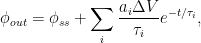


 s and
s and  s demonstrates what the folks meant above by saying that the residence time is a different animal from the Bern-formula time constants. If
  ,
,  , and
, and  , the mean steady-state residence time is 10, changing after the
  disturbance only a little, to between 9.7 and 10.4 according to the Bern formula. But, if
  is 5 instead of 1 to make the mean steady-state residence time 2 instead of 10, the Bern formula yields a residence time between 2.03 and 2.14–with the same time constants.
Although your initial comment seemed compelling at first, I have now been able to explain to myself what the folks above meant when they said that the residence time is a different animal from the Bern formula time constants. Just in case it helps any other layman out there who had the same difficulty I did, I’ll set forth what I think they meant.
Suppose that at steady state CO
But let’s change the scenario and add a slug
where
so that the CO$_{2}$ amount obeys the Bern formula:
Now, instead of a constant average residence time $V_{ss} /\phi_{ss}$, the residence-time average changes with time:
Putting numbers to those equations with the Bern numbers for the
Nick Stokes says:
And as to endless claims that all the new CO2 in the air has nothing to do with us – I’m sure Ferdinand Engelbeen will once again try to convey some sense on that. But the basic question – we’ve burnt about 400 Gt Carbon, and put it in the air. There is about 200 Gt more there than there used to be. If it isn’t ours, but came from the sea or wherever, then where did ours go?
This seems to confirm that it doesn’t stick around very long. If it’s true that we’ve emitted 400 Gt(the bulk of that in more recent years) and only increased the amount by 200 Gt.
” If it isn’t ours, but came from the sea or wherever, then where did ours go?”
Into the ocean and biosphere. Some of molecules that went into the ocean came out again to satisfy the outgassing. It’s assumed to be a linear system so you just work separately and add the results.
If there was no temperature rise, all but the last few percent of emissions eventually get absorbed, on the same basis as the C14 curve. If SST rises without any GHG emissions, whatever out-gassing required to restore equilibrium will happen. The net result is a linear superposition of the two effects.
I had this same discussion a few days ago elsewhere and someone said “it can’t be a sink and a source, you have to choose”.
Well, as explained it can. The net result is a linear superposition of the two effects.
BTW , I did a deconvolution of MLO with the 14y exponential and just looks a little rougher, nothing like the emissions data. I also did it with 2.6 (the shortest part of Bern model) and it got a bit rougher still … and looked even less like emissions.
” While they are remotely connected, the turnover of capital/goods says next to nothing about the gain or loss of that bussiness.”
Ferdinand, we love you, but this betrays a lack of business experience. The Carbon cycle has a huge (200gt) volume and it is a very profitable business. It feeds the biosphere. It is the World Bank for Carbon cash flow.
Couple things barely touched on; 14C is the heaviest and least likely isotope to be biologically absorbed. This should mean that it has the LONGEST residence time in the atmosphere. The oceans are supersaturated with 13 and 14C because these isotopes are biologically rejected both on land and preferentially washed in and in the oceans themselves where there is vast and unquantified biological activity
Ocean down welling uptake will vary with atmospheric isotopic composition at the edge of the ice near the poles. Upwelling outgassing along mid latitude and subtropical continental margins and along the ITC in the open oceans will return that isotopic signal to the atmosphere nearly a millennium later.
In a weird economic sense the isotopic skew of outgassing acts like the control of interest rates by the Federal Reserve. Spewing 12C is quantitative easing. Spewing 14C is like 18% interest.
mike g says: July 2, 2013 at 8:31 pm
“This seems to confirm that it doesn’t stick around very long. If it’s true that we’ve emitted 400 Gt(the bulk of that in more recent years) and only increased the amount by 200 Gt.”
This is described as the airborne fraction. As emissions have risen, it works out that about half of each increment appears to go into the ocean, half stays in the air. Of course, this is total net change. This is in a period of steady rise; whar would happen if the rise slowed hasn’t really been tested.
Joe Born says:
July 2, 2013 at 8:29 pm
But let’s change the scenario and add a slug of CO2 instantaneously at time …… etc etc …….
———————————————–
Do we know of any planets where that actually happens ?
“Bart says:
July 2, 2013 at 4:45 pm”
I agree with that assessment of Ferdinand’s confusion.
Tried to tell him something similar ages ago but it didn’t sink in.
There seems to be a general assumption that the mechanism for CO2 outgassing from the oceans is symmetric to the mechanism of CO2 being absorbed into the oceans. This assumtion implicitely means that this process only happens at the surface of the oceans, but is it really that simple?
Outgassing from the oceans is clearly a function of the temperature of the ocean and the CO2 concentration in the atmosphere and possibly to some extent a function of wind speed which increases/decreases the effective water surface area.
Absorption of CO2 back into the oceans is clearly symmetric to outgassing on the simplest level. On the other hand there are probably an additional and probably fairly important additional mechanism for extracting CO2 out of the atmosphere (I intentionally leave the biosphere out). It seems obvious to me that rain is a very efficient CO2 pump extracting CO2 from air. Why? The surface area of water drops in for example a thunder storm is extremely high and this is combined with a fairly long residence time of water drops at temperatures close to freezing even in tropical areas (dT=30K or more).
Does anybody have any interesting links to airplane measurements of CO2 inside rain clouds? I think the expected CO2 concentrations should be clearly lower than in the bulk of the atmosphere.
Are there measurements of CO2 concentration at surface levels in warm/cold areas of the earth? I expect the CO2 concentration should increase in tropical areas close to the surface during/after a thunder storm because CO2 was extracted from higher layers of the atmosphere and deposited on the ground where at least parts of the CO2 is released when the water heats up.
In cold areas the effect is probably weaker and a larger proportion of the CO2 ends up back in the ocean.
They can, because they measure different things. That is what all the objections to this posting are about. The 17 is the amount of CO2 molecules left from the pulse. The 73 is the excess of water.
I see that you have a good working analogy with your bucket with four chambers. Your model behaves as the formula, good job, but so do another with mixed gases which I will describe below:
Imagine a leaky bucket under an open tap. The bucket has four holes, one in the bottom and three just above the equilibrium level. The stream from the tap represents the natural CO2 sources and is constant. The leakage from the hole in the bottom represents natural sinks and is equal the natural sources.
All the dynamics caused by pouring a pulse of extra water in the bucket is explained by the three holes just above the equilibrium level. That means that the leakage from hole in the bottom in this model is independent of the water level.
I remind again of the Bern formula:
Each of the holes is connected to a closed tank on the outside of the bucket. The tank connected to the big hole representing lifetime of 1.186 years fill up after 18,6% of the pulse has drained.
The tank connected to the medium hole representing lifetime of 18.51 years fill up after 33.8% of the pulse has drained.
The tank connected to the smallest hole representing lifetime of 172.9 years fill up after 25.9% of the pulse has drained.
Observe that while this is going on the leakage from the hole in the bottom and the pouring from the tap, continues as before. That is the reason that the amount of molecules from the pulse is down to 17% after 5 years, but the amount of excess water is 73% of the pulse.
So to your objection about the saturation point. The answer is that in this model the saturation point is proportional to the pulse level, but it is fixed to the excess CO2 level measured in ppm. Ten times larger pulse gives ten times higher excess ppm level and ten times higher saturation point. The analogy to this is more like a very high leaky cylinder with small holes connected to small tanks all the way from the first equilibrium level and upwards to infinity.
So to the two scenarios above. Why does scenario 2 give less CO2 after 10 years although they had the same CO2 level in year 5? The answer is that in scenario 1, the tanks connected to the biggest holes have already filled up in year 5, so it only leaks through the smaller holes.
iopb
Should be the: “The 17 is the amount of CO2 molecules left from the pulse. The 73 is the excess of CO2 level from the pulse”
philincalifornia: “Do we know of any planets where that actually happens ?”
If you’ll grant me some leeway on “instantaneous,” I’m guessing earth. I assume small slugs of CO2 are are frequently added in period of time that are minuscule compared with the Bern time constants. I did it myself when I let blocks of dry ice sublime.
In any event, the Bern formula tells what would happen if such an instantaneous impulse were to occur, and what I (think I) showed is that its time constants are consistent with a wide range of residence times.
tumetuestumefaisdubien1 says:
July 2, 2013 at 4:31 pm
its partial pressure there is 44.0095[CO2 molar weight]/28.97[air molar weight] x 0.0004 = 0.000607 at
You ar confusing partial pressure for a mass ratio with ppmv, which is already a volume ratio and thus = partial pressure. For 400 ppmv and 1 atm that is thus near 400 microatm, be it a few % less as the ppmv is expressed in dry air. Thus one need to take into account the % water vapour.
there’s ~0.001328 g of CO2 solved in surface ocean layer 1cm^2 of 16.6 C sea water which weights ~1.026 grams, therefore the partial pressure of the CO2 in the water is 0.00133/1.026 = ~0.00129 at.
Not right. Most of the dissolved CO2 is in the form of bicarbonates and carbonates. These play not the slightest role in the pressure of the remaining (less than 1%) free CO2 in seawater. What is done is measuring CO2 in the air in close contact with seawater, either by bubbling air through the water or spraying seawater in air. That gives the equilibrium CO2 levels at the temperature of the mixture. That is used to calculate the fluxes between oceans and atmosphere, as the flux is directly proportional to the partial pressure difference between (equilibrium) CO2 in seawater and in the atmosphere.
the partial pressure of the CO2 in the mean temperature sea water is more than twice as high than the CO2 partial pressure in the air.
No, the partial pressure of CO2 in the oceans in average is 7 microatm less than in the atmosphere, see:
http://www.pmel.noaa.gov/pubs/outstand/feel2331/exchange.shtml
That is based on several million direct measurements of CO2 partial pressure measurements in the oceans by regular cruises, commercial seaships, buoys and a few fixed stations.
Gail Combs says:
July 2, 2013 at 4:40 pm
Because the data passed through a filter (ice cores) that clipped the peaks.
Filtering clips peaks and drops alike. Thus IF there were huge peaks at all, there were huge drops alike. But as we already see low average values of around 180 ppmv, that would mean starvation of a lot of plants…
Further, your first link shows the error from the late Jaworowski: the so called erronic shift of 83 years to splice the ice core record and the Mauna Loa data together. Jaworoski used the ice age column in the data table of Neftel, not the gas age column. Anybody remotely knowable of ice cores knows that the average gas age in the enclosed bubbles is (much) youger than the surrounding ice, simply because the pores remain open to the atmosphere for years after the snow was deposed…
About Glassman, it is near impossible to have a discussion with him, as for every argument he buries you with relevant and irrelevant answers, so that it costs you weeks just to unravel what is relevant and what not… I did give up reacting there…
A question to Ferdinand Engelbeen :-
– Can you or anyone else explain why “natural” CO2 levels in the atmosphere are currently 200-280 ppm (depending on the state of glaciation). Why for example are they not 2000 ppm or 20 ppm ?
– The build up of O2 through photosynthesis is limited to ~18% by the spontaneous combustion of forests. Is it not likely that photosynthesis also forces a lower limit for CO2 because much below ~280 photosynthesis slows down and stops ?
– Is there a natural upper limit for CO2 levels ? I suspect that there must be, because volcanic activity was orders of magnitude greater in the past yet CO2 levels have always been (relatively) low. As CO2 levels rise so too does the rate of photosynthesis. More plant growth pumps more CO2 into the ground speeding up rock weathering thereby lowering CO2 levels.
Things seem to have calmed down, so I feel safe to emerge from under my log…
I would like to introduce a point that does not seem to have been mentioned yet, possibly because it is irrelevant, but here goes. The Mauna Loa CO2 data shows a slow steady increase in atmospheric CO2 when averaged over the long term, but in fact there is a seasonal fluctuation that is quite spectacular – the actual rate of change of CO2 concentration is always much greater than the smoothed line – either positive or negative. I assume that industrial CO2 production is fairly non-seasonal, so these rapid changes are natural – biological and physical processes. The thing that really strikes me is the slope – the atmospheric CO2 concentration is capable of much faster change than we see long term. I am particularly interested in the down slope, how does CO2 disappear from the atmosphere so quickly? Does this in any way inform about the nature of the sinks?
NickStokes: “This is described as the airborne fraction. As emissions have risen, it works out that about half of each increment appears to go into the ocean, half stays in the air. Of course, this is total net change. This is in a period of steady rise; whar would happen if the rise slowed hasn’t really been tested.”
Indeed Nick, that is the problem, we have monotonic rise in temperature, a monotonic rise in emissions and two physical relationships which work in the same direction. There is clearly going to be some mix of the two, the problem is to work out the proportion of each. We have one equation and two unknowns. What we need is a second relationship to provide enough information. Then we have two equations, two variables and the problem is in principal solvable.
That is why I keep banging on about rate of change. The rate of change response will not be the same for both relationships and should provide a tie breaker.
Now the linear response model will mean that effectively there will some component of d/dt(CO2emm) in CO2atm : but both are hit by a low pass filter with its half power point at w*tau=1
http://climategrog.wordpress.com/?attachment_id=402
Now even taking the shortest Bern time constant that give half power at 2*pi*1.18 =7.4 years
So although the HF response will be dominated by d/dt(CO2emm) it gets low-pass filtered, so it is only the intermediate frequencies around 10 years that will get be significant in CO2atm. Far Longer if the time constant of the bomb curve is used.
This cannot explain the strong correlation with climatic variable such as global SST and arctic atmospheric pressure.
http://climategrog.wordpress.com/?attachment_id=259
http://climategrog.wordpress.com/?attachment_id=233
I have not got a method to extract an estimation of the ratio yet but the means is there to get an answer based on reliable recent data rather than making spurious assumptions about how 10k year old ice core data from a massive change in climate state over thousands of years relates to what we see in the 50 years.
Bart says:
July 2, 2013 at 4:45 pm
I think I see now the source of your confusion. It is a temperature dependent pump, in that its output is modulated by temperature. But, temperature is not the only process governing the flow. You are thinking that the upwelling waters have the same CO2 content as the surface waters before they warmed. But, there is no such constraint.
No, I know that the upwelling waters are far richer in CO2 than the surface waters. Even without a change in temperature, the upwelling at the equator will release a lot of CO2, only slightly modulated by temperature changes. An increase of 1 K in temperature at the upwelling places will increase the CO2 flux from ocean to the atmosphere with less than 5%, all other variables remaining the same.
Increasing surface temperatures merely speeds up the process or, if they decrease enough, bring it to a halt.
The equilibrium pressure of seawater CO2 at the upwelling places is about 750 microatm. Of the atmosphere it is ~400 microatm. To stop the outgassing, you need to bring the 750 microatm in the ocean surface down to 400 microatm. The temperature effect on the pCO2 of the oceans is about 16 microatm/K, thus you need a drop of 22 K to stop the equatorial outgassing…
Of course, that is only halve the story, as at the other side of the world, the sinks react in opposite ways on temperature changes.
The main point is that temperature only has a minor role in the total fluxes involved (my own estimate: some 40 GtC/yr as CO2 is transported from the equator to the poles). A global increase of 1 K would increase the outgassing at the equator with some 2 GtC/yr and decrease the uptake near the poles with about the same amount/yr. That causes an increase of 4 GtC/yr or 2 ppmv per year. That is about what we see today.
The problem is that that only is true for the first year. When the CO2 levels in the atmosphere increase, the difference in pCO2 between atmosphere and oceans is reduced at the upwelling places and increased at the downwelling places. With an increase of only 16 ppmv, the fluxes are restored to what they were before the temperature increase.
That makes it impossible that a sustained change in temperature can cause a continous imbalance of CO2 in/outflux, resulting in a continuous increase of CO2 in the atmosphere. In reality, a change of CO2 in the atmosphere caused by temperature stops when the flux (un)balance is restored.
Other influences may induce non-temperature related changes in CO2 fluxes, but we were discussing the unique influence of temperature on the CO2 levels in the atmosphere, not the other possibilities.
Ferdinand said:
“Of course, that is only halve (sic) the story, as at the other side of the world, the sinks react in opposite ways on temperature changes.”
Not at the same time they don’t. In the late 20th century upwelling CO2 rich water (possibly from the Dark Ages 1500 years ago) was arriving at the surface at a time of active sun with low global cloudiness and increased sunlight on the ocean surfaces so the outgassing was most certainly not being offset by enhanced absorption elsewhere. The increased sunlight reduced the absorption capability of the entire globe including at the poles.
Ferdinand also said:
“Other influences may induce non-temperature related changes in CO2 fluxes”
Well there you go then.
Every aspect of the carbon cycle is indeed in a state of non temperature related variability in CO2 flux and we just don’t have a grip on it as Murry Salby rightly pointed out.
Ferdinand’s simplistic assertions and conclusions derived from his inadequate assumptions therefore cease to have any persuasive capability.
So many words, so much time. All wasted.
Jim Turner: “I am particularly interested in the down slope, how does CO2 disappear from the atmosphere so quickly? Does this in any way inform about the nature of the sinks?” and
and  set forth there as obeying the Bern formula but rather some values whose lowest harmonics are
 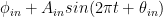 and
and  , where the sinusoids represent the first harmonic of the earth’s “breathing” on which you remarked.
It probably does, but don’t think it give us much on which to base the validity of the Bern formula at issue, although I’m no scientist, so you may want to read my reasoning critically.
That reasoning is basically my LaTeX-equations-containing comment above with the following refinement. The values of CO2 flux are not simply the
With that change, I believe the reasoning still applies, so I don’t think the earth’s respiration tells us much about whether the Bern formula is valid.
clivebest says:
July 3, 2013 at 4:13 am
Can you or anyone else explain why “natural” CO2 levels in the atmosphere are currently 200-280 ppm (depending on the state of glaciation). Why for example are they not 2000 ppm or 20 ppm ?
The main sink since millions of years ago is the deposit of CO2 in huge chalk layers at the bottom of the seas. Some of it was uplifted and is visible as carbonate rock in all its forms. The second (mostly older) storage is coal and more recent browncoal, peat and other (semi-)permanent carbon deposits. Since a few million years ago, it seems that temperature is the main driver of CO2 levels: there is a relative stable correlation between temperature and CO2 levels (the latter lagging) over the past 800 kyrs and beyond. That means that non-temperature related releases (volcanoes) and uptakes (rock weathering) are relative balanced.
2000 ppmv is not seen, because that was used by coccoliths to form their skeleton and now rests on the bottom of the oceans.
20 ppmv is not seen, as that would include starvation of vegetation, thus eliminating one of the main sinks…
Is it not likely that photosynthesis also forces a lower limit for CO2 because much below ~280 photosynthesis slows down and stops ?
That is probably the lower limit, but you never know what could happen if one of the sources (volcanoes, bacteria) reduce their output further…
Is there a natural upper limit for CO2 levels ? I suspect that there must be, because volcanic activity was orders of magnitude greater in the past yet CO2 levels have always been (relatively) low. As CO2 levels rise so too does the rate of photosynthesis. More plant growth pumps more CO2 into the ground speeding up rock weathering thereby lowering CO2 levels.
In part the oceans, in part the biosphere are the main sinks for CO2. But the fastest sink, the ocean surfaces have a limited capacity and both deep oceans and more permanent storage in the biosphere have a (near) unlimited storage, but are limited in uptake speed. Thus much depends of the speed of release of the extra CO2…
Stephen Wilde says:
July 3, 2013 at 6:03 am
The increased sunlight reduced the absorption capability of the entire globe including at the poles.
Stephen, CO2 fluxes in/out the oceans are directly proportional to pressure differences, not to sunlight. The latter may induce temperature changes of the ocean surface and therefore increase the CO2 pressure in the ocean. But there is no direct influence of sunlight on CO2 escape from the surface or uptake by the surface. If you have information of the contrary, I like to know that.
Every aspect of the carbon cycle is indeed in a state of non temperature related variability in CO2 flux and we just don’t have a grip on it as Murry Salby rightly pointed out.
Wait a minute. Bart, Salby and now Pettersson all discuss the influence of temperature as cause of the current increase of CO2. My take is that the temperature increase since the LIA is good for maximum 16 ppmv on good grounds (Henry’s Law) of the 100 ppmv increase (70 ppmv since Mauna Loa). Their take is that a small sustained increase in temperature can induce a continuous increase of CO2 in the atmosphere. Which is physically impossible.
If you want to discuss other probable sources, we can do that. But that is not the object of this discussion. Take e.g. your remark:
In the late 20th century upwelling CO2 rich water
If that water was from the “Dark ages” or from the MWP or from the LIA, it may contain some extra CO2 or less CO2. The atmosperic difference between the MWP and LIA was 6 ppmv CO2. That is what you may get back. Not more than that.
Ferdinand Engelbeen says:
> If that water was from the “Dark ages” or from the MWP or from the LIA, it may contain some extra CO2 or less CO2.
Indeed it may. The ocean is full of life, and the current concentration of dissolved CO2 (along with carbonates and bicarbonates) depends on the overall stoichiometry of ocean metabolism, in addition to surface and subterranean sources and sinks. None of which is bound to be constant. Do we know what the balance was between aerobic / anaerobic / photosynthetic life forms 1000 years ago?
“If you want to discuss other probable sources, we can do that. But that is not the object of this discussion.”
The alleged temperature connection is not about temperature change but temperature level. The correlation is between CO2 change and temperature (not change). Constant (annualy averaged) temperatures cause change in atmospheric CO2.
Ferdi says: “The temperature effect on the pCO2 of the oceans is about 16 microatm/K, thus you need a drop of 22 K to stop the equatorial outgassing…”
So at what time were the ocean surface 22K cooler than today to that CO2 to get there in the first place?!
You confidently assert there figures but you understanding is clearly erroneous on some key points. You like to focus on 766-400/(750-400), what is the other end of the scale where that ration gets bigger?
Where do you get your 16ppmv/K ?
Ferdi says: ”
No, the partial pressure of CO2 in the oceans in average is 7 microatm less than in the atmosphere, see:
http://www.pmel.noaa.gov/pubs/outstand/feel2331/exchange.shtml
That is based on several million direct measurements of CO2 partial pressure measurements in the oceans by regular cruises, commercial seaships, buoys and a few fixed stations.”
That’s useful (assuming the averaging is done properly). That reflects the ongoing imbalance between out-gassing and absorption of continued emissions.
Bart says:
July 2, 2013 at 5:37 pm
It does not match this observation. It does not match this one.
Your other observations are equivocal. These are not
The first graph is partly right (the short term variability), partly curve fitting by choosing an arbitrary zero line which matches the trend. A similar matching against an arbitrary zero line which was done by Salby.
The second graph is a typical example of “how to mislead with graphs by choosing the scales”. The emissions and airborne part can be seen on the same scale and that tells a different story:
http://www.ferdinand-engelbeen.be/klimaat/klim_img/dco2_em2.jpg
or accumulated:
http://www.ferdinand-engelbeen.be/klimaat/klim_img/emissions.gif
or accumulated and compared to the temperature trend:
http://www.ferdinand-engelbeen.be/klimaat/klim_img/temp_co2_acc_1900_2004.jpg
Seems to me that matching the temperature trend with the increase of CO2 over the periods before 1960 is not such an easy task…
Edim says:
July 3, 2013 at 6:45 am
The alleged temperature connection is not about temperature change but temperature level. The correlation is between CO2 change and temperature (not change). Constant (annualy averaged) temperatures cause change in atmospheric CO2.
No, that is physically impossible. A fixed increase in temperature above a zero line will give a constant inflow of CO2 into the atmosphere. That is what Bart and Salby say.
But such a continuous inflow will increase the CO2 levels in the atmosphere and the increase in the atmosphere will decrease the inflow of CO2 from the oceans at the equator and increase the outflow of CO2 into the cold Arctic waters (and in alveoles of leaves). Thus it simply is impossible that the inflow of CO2 remains constant for a constant temperature difference…
Ferdi says: “But such a continuous inflow will increase the CO2 levels in the atmosphere and the increase in the atmosphere will decrease the inflow of CO2 from the oceans at the equator and increase the outflow of CO2 into the cold Arctic waters (and in alveoles of leaves). Thus it simply is impossible that the inflow of CO2 remains constant for a constant temperature difference…”
Which means that the process needs to be modelled by at least a first order differential equation. This is exactly what Gösta Pettersson has done and has calibrated against known good quality data.
Glad to see you are a finally getting the message. (Even if you haven’t realised yet)
“No, the partial pressure of CO2 in the oceans in average is 7 microatm less than in the atmosphere, see:”
This is also because plankton actively pump it out of the water and into the atmosphere.
Gene Selkov says:
July 3, 2013 at 7:12 am
Do we know what the balance was between aerobic / anaerobic / photosynthetic life forms 1000 years ago?
Indeed we have not much knowledge of ocean chemistry and biology, execept from deposits on the ocean floor and corals etc…
But we have quite good knowledge of the CO2 levels in the atmosphere as result of all the CO2 fluxes together: an increase or decrease of about 8 ppmv/K over the past millenium with a resolution of ~20 years, up to 800 kyears with a resolution of 560 years.
That shows very little variation over the past 1000 years, far from the over 100 ppmv/K we see over the past 50 years.
Thus whatever the cause of the increase, we may say with confidence that the current increase is unique over the past 800 kyears and not caused by any known natural source, including the oceans.
Ferdinand Engelbeen,
I admire your tenacity; after seeing several similar (erroneous) attribution arguments over the past few years, I completely gave up on trying to explain the physics to those who insist 1C warming of the ocean surface can raise atmospheric CO2 levels by 120 PPM. I have never once seen a person persuaded by the overwhelming evidence and the correct physical explanations if they start by saying that ocean warming caused increases in CO2 (not fossil fuel burning). Looks like Willis has given up as well… a prudent choice I think.
A discussion about the accuracy of the Bern model would be more interesting. I suspect that the Bern model is far from correct because it seems to ignore (or greatly discount) important physical processes involved in CO2 absorption (solubility pump, biological pump). These processes ought to guide the model’s structure. A multiple pool model with adjustable lag constants can for sure be made to fit the data, but may not make good predictions.
Greg Goodman says:
July 3, 2013 at 7:28 am
This is exactly what Gösta Pettersson has done and has calibrated against known good quality data.
Glad to see you are a finally getting the message. (Even if you haven’t realised yet)
Except that Gösta has used the 14C bomb spike, which is representative for the exchange rate, not the real decay rate for an extra addition of CO2 mass (14 C is negligible in mass). Different decay times. That for extra CO2 is ~55 years, that of 14C is ~14 years. See:
http://www.john-daly.com/carbon.htm
The difference is that the increase in the atmosphere is 50/50 human/natural with bomb spike decay rates and 100% human with mass decay rates.
I see issues with the claims of a monoexponential shape of the bombtest curve, and of thermal outgassing.
As for the shape of the bombtest curve: It appears to me as about to pass below zero rather than continue an exponential decay shape. Also, it appears to me that the last shown datapoint is 43 years after atmospheric nuclear explosions ended, which is 2006.
As for thermal outgassing: I see a missing factor here. Solubility of a gas in a liquid not only varies inversely with temperature, but also directly with increase of the partial pressure of the gas.
That would explain plausibility of the following link’s showing that in recent decades, oceans have been removing CO2 from the atmosphere instead of adding it:
http://www.tyndall.ac.uk/global-carbon-budget-2010
One thing about the rate of nature *removing* CO2 despite the heat is that atmospheric lifetime of CO2 is probably less than the long times claimed by advocates of existence of AGW. I seem to think that with nature removing on average about 40% of human-added CO2 in any short time period in the past few decades, atmospheric lifetime would be about (60/40) or 1.5 times the roughly 28 year time constant in the roughly exponential growth of atmospheric CO2.
Nick Stokes says:
July 2, 2013 at 10:50 pm
“As emissions have risen, it works out that about half of each increment appears to go into the ocean, half stays in the air.”
Nick, you are chanting cant and narrative. The narrative is failing. Tiime to do some independent thinking on your own.
“…wha[t] would happen if the rise slowed hasn’t really been tested.”
But, what would happen if it accelerates has. The apparent “airborne fraction” is decreasing. If you were not wedded to the narrative, you would see that it is in a crisis.
Ferdinand Engelbeen says:
July 3, 2013 at 3:18 am
“Filtering clips peaks and drops alike.Thus IF there were huge peaks at all, there were huge drops alike.”
Ouch! Ferdinand, your logic is truly twisted. Just because drops would have been filtered if they were there does not mean they were there.
Ferdinand Engelbeen says:
July 3, 2013 at 5:41 am
“Of course, that is only halve the story, as at the other side of the world, the sinks react in opposite ways on temperature changes.”
But, in the same direction with regard to maintaining CO2 in the atmosphere. Sources expand, sinks contract. Result: greater atmospheric concentration.
“The main point is that temperature only has a minor role in the total fluxes involved.”
That may or may not be the case. But, so what? It is the temperature modulated pumping of CO2 rich waters into the system which is the main driver.
Ferdinand Engelbeen says:
July 3, 2013 at 6:29 am
“Bart, Salby and now Pettersson all discuss the influence of temperature as cause of the current increase of CO2.”
You have misinterpreted. It is temperature modulated, caused by the offset of surface temperature from the level which would be required for equilibrium. But, the equlibrium temperature is set by the input flux from upwelling waters.
Ferdinand Engelbeen says:
July 3, 2013 at 7:10 am
“The first graph is partly right (the short term variability), partly curve fitting by choosing an arbitrary zero line which matches the trend.”
The curve fit matches the trend in the rate of CO2, as well as the variablity. The rate of emissions also has a trend. But, the trend in the rate of CO2 is already accounted for by the temperature relationship. Hence, there is no room for significant influence of emissions.
You would have a point af the rate of emissions had been constant. Then, the choice of baseline for the temperature relationship would be ambiguous with the emissions. But, since the emissions also have a trend, and the trend in measurements is already explained by the temperature relationship, we can rule out significant forcing from the emissions.
“The second graph is a typical example of “how to mislead with graphs by choosing the scales”.”
There is an unambiguous divergence between the rate at which emissions are being generated and the rate at which measured CO2 is increasing. It’s only going to get worse for you as time goes on, because temperatures are going down, and measured CO2 is tracking that decrease, while emissions continue accelerating.
Donald L. Klipstein says:
July 3, 2013 at 8:05 am
“That would explain plausibility of the following link’s showing that in recent decades, oceans have been removing CO2 from the atmosphere instead of adding it:”
This “mass balance” argument has been discredited. This is a feedback system. Static analysis does not apply.
Steve Fitzpatrick says:
July 3, 2013 at 7:50 am
“I completely gave up on trying to explain the physics to those who insist 1C warming of the ocean surface can raise atmospheric CO2 levels by 120 PPM.”
No, you gave up listening, if you ever started. Your argument is a strawman. See above.
Steve Fitzpatrick says:
July 3, 2013 at 7:50 am
Thanks for your kind words. I am afraid that Willis has given up, maybe his blood pressure got too high…
I suspect that the Bern model is far from correct because it seems to ignore (or greatly discount) important physical processes involved in CO2 absorption (solubility pump, biological pump). These processes ought to guide the model’s structure.
I fully agree. As far as remember, the Bern model was based on the burning of enormous amounts of fossil fuels: all oil and gas and lots of coal. The initial amounts were calculated for 3000 and 5000 GtC. We are currently at 370 GtC…
At 3000 GtC, some of the terms make sense, not at lower emissions. The constant term is only applicable if all other sinks are balanced or saturated at that higher level. That will never be for e.g. more permanent storage in vegetation, as the coal deposits prove. If the human emissions would stop today and all until now emitted CO2 sinks in the oceans (at a decay rate of ~55 years), after a few centuries the levels in the atmosphere would be near equilibrium and what returns from the oceans gives less than a few ppmv increase in the atmosphere.
This moment there is not the slightest sign that any of the main sinks (oceans and vegetation) are saturating, to the contrary. Thus indeed, the Bern model is wrong…
http://www.pmel.noaa.gov/pubs/outstand/feel2331/exchange.shtml
” The pCO2 in surface seawater is known to vary geographically and seasonally over a range between about 150 µatm and 750 µatm, or about 60% below and 100% above the current atmospheric pCO2 level of about 370 µatm. ”
So that give the other end of the scale Ferdinand does not want to talk about. So let’s have a look at some intermediate values based on his 16ppmv/K (where ever that comes from)
Xi = X/(750-400)*(766-400) = 1.046 X
Xi = X/(450-400)*(466-400) = 1.320 X
Xi = X/(420-400)*(436-400) = 1.800 X
Xi = X/(350-400)*(366-400) = 0.680 X
Xi = X/(150-400)*(166-400) = 0.936 X
So his much quoted 750 µatm implying 4.6% increase from the warmest waters is hardly representative and that calculation will go infinite as it crosses 400ppmv since it is a proportional change. In fact the colder, acting in the same sense, are more important than the warm waters as I already suggested. This may go someway to explaining the correlation with Arctic Oscillation that I found.
http://climategrog.wordpress.com/?attachment_id=231
So back to the supposed 16ppmv/K. Unless I missed it Ferdi has still explained where he got it but let me guess. 100ppmv / 6 K for last deglaciation = … fine.
So this is a classic case of warmist circular logic. We’ll assume that a huge swing between different pseudo-stable climate states with CO2 generally regarded as being a significant +ve feedback is representative . Glaciation has half the world under ice the rest subdued by much lower temp and lower CO2 BUT let’s not worry, assume that is the same as current climate with Arctic ice a ” death spiral” . Let’s also assume that there is 0.00000000% diffusion and that these ice records were and still are an accurate reflection of climate at that time. After all it would be “immoral” to question the reliability of ice cores (thanks Gail ).
where was I? Oh yes, so we’ll assume all that and then go on to prove the temperature cannot cause more than a few 10s of ppmv of change in CO2. Which “proves” we were right in our assumptions !
QED.
Like the nearly the whole of climate science for the last 30 years, you start by assuming your result , then set out to prove it.
Ferdi: says “I fully agree. As far as remember, the Bern model was based on the burning of enormous amounts of fossil fuels: all oil and gas and lots of coal. The initial amounts were calculated for 3000 and 5000 GtC. We are currently at 370 GtC…
This moment there is not the slightest sign that any of the main sinks (oceans and vegetation) are saturating, to the contrary. Thus indeed, the Bern model is wrong…”
So we need a new one. Like the one proposed here perhaps. Based on real data , not on trying to recreate prejudiced assumption about the future.
Bart says:
July 3, 2013 at 8:14 am
Ouch! Ferdinand, your logic is truly twisted. Just because drops would have been filtered if they were there does not mean they were there.
If there were peaks, then there were drops. Ice cores filter, but don’t change the average over the resolution period. Maybe if the peaks were short and the drops were long, but that is quite unlikely.
Anyway the current increase of 100 ppmv over 160 years would have been detected in every ice core back to 800 kyears ago.
That may or may not be the case. But, so what? It is the temperature modulated pumping of CO2 rich waters into the system which is the main driver.
I don’t know of any temperature process that increases the upwelling of deep ocean waters. The opposite happens: wind drives the upwelling and causes temperature changes. That is what ENSO does, including the extra upwelling of CO2. Nothing to do with a permanent increase in upwelling from a permanent increase in temperature.
Further, if there is more upwelling, there is more downwelling too. All what happens is more circulation. Any unbalance would be countered by a small change in the atmosphere with a short decay rate.
In no way such an increase would be continuous.
That is the main point where it goes wrong:
No matter the effect of temperature on the oceans: increased temperature, increased upwelling or increases in concentration (from the far past), its effect on influxes and outfluxes would be countered by a small change of the CO2 levels in the atmosphere.
The curve fit matches the trend in the rate of CO2, as well as the variablity. The rate of emissions also has a trend. But, the trend in the rate of CO2 is already accounted for by the temperature relationship.
The short term variability is accounted for, but the trend fit is completely ambiguous: that can come near 100% from the emissions to near 100% from temperature.
There is an unambiguous divergence between the rate at which emissions are being generated and the rate at which measured CO2 is increasing.
So what? Some of the sinks may increase thanks to stalled temperatures, the melting of the Arctic ice may help by an increasing cold area,… That simply is natural variability.
I have digitised the data:

If the process is not monoexponential, the data are not good enough to show that.
Greg Goodman says:
July 3, 2013 at 8:44 am
Thanks. I never bothered looking into Ferdinand’s calculation because A) it is moot B) I suspected he was using circular logic as you describe.
Ferdinand Engelbeen says:
July 3, 2013 at 10:08 am
“If there were peaks, then there were drops.”
Nonsense. Drops from the peaks, yes. Drops below some nominal level, no.
“I don’t know of any temperature process that increases the upwelling of deep ocean waters.”
The concentration of the upwelling waters is determined by both temperatures at the time the waters originally downwelled and any other additions or subtractions which took place during its long trek through the depths.
“Further, if there is more upwelling, there is more downwelling too.”
Not until atmospheric concentration has increased. A temperature increase futher constricts downwelling. With constant upwelling of CO2 rich waters, you get a constant pumping of CO2 into the atmosphere.
Open your eyes, Ferdinand. This is all evident in the data.
“No matter the effect of temperature on the oceans: increased temperature, increased upwelling or increases in concentration (from the far past), its effect on influxes and outfluxes would be countered by a small change of the CO2 levels in the atmosphere.”
Sorry, no, that is just not so.
“…but the trend fit is completely ambiguous: that can come near 100% from the emissions to near 100% from temperature.”
No. It cannot. You cannot arbitrarily pick and choose which parts you want to keep, and which you want to dismiss. You either accept it all, or none. Nature does not have any mechanisms to juggle things as you prescribe, and the odds that it would even if it could are vanishingly small.
“That simply is natural variability.”
Funny how nature only varies in a way to confirm your bias.
Ferdi says: “The equilibrium pressure of seawater CO2 at the upwelling places is about 750 microatm. Of the atmosphere it is ~400 microatm. To stop the outgassing, you need to bring the 750 microatm in the ocean surface down to 400 microatm. The temperature effect on the pCO2 of the oceans is about 16 microatm/K, thus you need a drop of 22 K to stop the equatorial outgassing…”
And the world have NEVER been 22K colder that it currently is, so you value of 16 microatm/K or 16 ppmv/K is erroneous.
I realise it’s a bit busy in here, but that assumption is the cornerstone of your position, you need to deal with it.
Greg Goodman says:
July 3, 2013 at 8:44 am
Sorry Greg, but I have some problems to understand what you mean.
Maybe some background may help:
The main inflow of CO2 in the atmosphere from the oceans is near the equator and especially around the upwelling places.
The main outflow of CO2 into the oceans is in the NE Atlantic where the main sink place of cold water takes place.
The mid-latitudes may be sinks or sources, depending of (seasonal) temperature.
So that give the other end of the scale Ferdinand does not want to talk about.
As you are quite new here, I have discussed that several times, but didn’t want to repeat that every time again. The effect of an increase in temperature in polar waters is that less CO2 is going into the oceans, as you have calculated. That is a 7% decrease in outflux.
These two are what is important, as they reflect the continuous exchange between the atmosphere and the deep oceans. The intermediate waters have no direct access to the deep oceans, they are in direct exchange with the atmosphere, but the uptake/release is limited in capacity to 10% of the change in the atmosphere. That is the result of the buffer factor in the oceans, the so-called “Revelle factor”. The 30% increase in the atmosphere over the past 160 years resulted in a 3% increase of carbon in the ocean surface layer or 30 GtC increase for the 1000 GtC in the “mixed layer”.
What happens if suddenly all oceans increase 1 K in temperature?
Immediately the equilibrium pressure of all ocean waters will increase with 16 microatm everywhere.
Quite fast (6-months lag) the levels in the atmosphere will increase in CO2 content. Partly by more releases, partly by less sinks. Once the increase in the atmosphere reaches 16 ppmv (1-3 years decay time), all the previous (seasonal and continuous) fluxes are restored in their previous state and no increase in atmospheric CO2 will continue due to the temperature increase.
So back to the supposed 16 ppmv/K
The 16 ppmv/K simply is the measured change in atmospheric CO2 partial pressure (~level) when seawater is brought into equilibrium with a small amount of air. That is a rough figure and is higher at higher levels and lower at lower CO2 levels. Currently they seem to calculate the change as a fixed % of the pCO2 level, see:
http://www.ldeo.columbia.edu/res/pi/CO2/carbondioxide/text/Palmer_methods.pdf
Greg Goodman says:
July 3, 2013 at 8:44 am
After all it would be “immoral” to question the reliability of ice cores (thanks Gail ).
I had several discussions with Gail and others, so I don’t react every time again, but as you probably haven’t seen them…
If you want to rely on the work of the late Jaworowski, that is up to you. But please, first have a look at my comment:
http://www.ferdinand-engelbeen.be/klimaat/jaworowski.html
Jaworowski’s knowledge of ice cores ended in 1992. Most of his objections were already refuted in 1996 by the work of Etheridge e.a. on three ice cores at Law Dome, with three drilling techniques (wet and dry). The result:
http://www.ferdinand-engelbeen.be/klimaat/klim_img/law_dome_overlap.jpg
Besides insisting that the average age of the gas in the bubbles is the same as in the surrounding ice, he closed the door for me by insisting that CO2 migrates in ice from low levels to high levels. As far as I know, there is no reverse osmoses at work between ice at 2000m and 1999 meter depth.
But think one moment about what would happen to the nice temperature-CO2 ratio for each glacial-interglacial transition back in time, if there was substantial migration: would the CO2 levels not gone completely flat after 800 kyears when 90% of the time the temperatures and CO2 levels are much lower?
Further about migration in (relative “warm”) ice cores:
http://catalogue.nla.gov.au/Record/3773250
The estimated diffusion (calculated from remelt layers) means a broadening of the resolution from 20 to 22 years at medium depth and from 20 to 40 years at full depth…
Gene Selkov says:
July 3, 2013 at 10:29 am
Can you make the data available as well as the graph? What about the other data (Jungfraujoch, Krakow, etc.)?
Lance Wallace says:
> Can you make the data available as well as the graph? What about the other data (Jungfraujoch, Krakow, etc.)?
Sorry, I’ve just departed from work and left the table on a machine that I can’t access. I’ll post it first thing in the morning. I’ll add the other data too.
Greg Goodman says:
July 3, 2013 at 12:09 pm
And the world have NEVER been 22K colder that it currently is
Greg, that was a reaction on Bart, July 2, 2013 at 4:45 pm:
When upwelling waters are CO2 enriched beyond the level of surface waters, that CO2 will be pumped into the atmosphere when the waters surface, regardless of the prevailing temperature. Increasing surface temperatures merely speeds up the process or, if they decrease enough, bring it to a halt. Right now, bringing it to a halt would require a drop in global temperatures of about 0.25 degC.
On which I reacted that to stop the upwelling of CO2 from the deep ocean waters you need a drop of 22 K. A drop of 1 K would only reduce the release of CO2 from the deep oceans with 6%. A drop of 0.25 K hardly with 2%…
It fully shows the result of relying on a small change in temperature as cause of a huge continuous increase or decrease of CO2 in the atmosphere.
And again, a small decrease or increase of CO2 in the atmosphere would restore the previous fluxes after a temperature change.
Bart says:
July 3, 2013 at 10:40 am
Thanks. I never bothered looking into Ferdinand’s calculation because A) it is moot B) I suspected he was using circular logic as you describe.
No problem with that. Only one question:
– If the CO2 levels increase due to an increase in temperature (direct or indirect), does that have an effect on the fluxes between the oceans and the atmosphere or not?
Ferdinand Engelbeen says:
July 3, 2013 at 12:46 pm
“A drop of 0.25 K hardly with 2%…”
I estimated 0.25 degC from here. That is roughly the amount of change in global temperature average needed to achieve the equilibrium temperature.
You are thinking about this incorrectly, and therefore making incorrect conclusions. The oceanic CO2 pump relies on a lot more than just current surface temperatures. I depends on the history of the entire circulation over the last millennium.
It depends… my fingers seem lazy today.
Bart says:
July 3, 2013 at 1:12 pm
You are thinking about this incorrectly, and therefore making incorrect conclusions. The oceanic CO2 pump relies on a lot more than just current surface temperatures. I depends on the history of the entire circulation over the last millennium.
Bart, you are mixing different variables, which confuse the discussion. The whole discussion is about the continuous extra inflow of CO2 due to an increase in temperature.
If there was a change in total deep ocean inflow or concentration of the inflow, these do influence the CO2 influx, regardless of the temperature. The temperature increase only gives a small extra percentage of CO2 influx (and a small percentage less in CO2 outflux).
Thus in such cases, the main change in the atmosphere is from the changes in upwelling and/or concentration, not from temperature.
Rest my question about the impact of any change in CO2 level of the atmosphere on the fluxes…
Ferdinand Engelbeen says:
July 3, 2013 at 1:49 pm
“Thus in such cases, the main change in the atmosphere is from the changes in upwelling and/or concentration, not from temperature.”
Yes, and no. It is a temperature dependent flow. If the current temperature were the equilibrium temperature, it would cease pumping into the atmosphere.
Anyway, sorry to have to break off, but as you may or may not know, it is a holiday weekend here in the US, and my family is pushing me to get out the door. Until next time…
Thanls for the replies, Ferdi.
“On which I reacted that to stop the up-welling of CO2 from the deep ocean waters you need a drop of 22 K. ”
Because of the large difference of SST where they come up. OK.
So we are all agreed that the out-gassing will continue as long a the water continues to rise. I think that was the point Bart was making.
F: ” The effect of an increase in temperature in polar waters is that less CO2 is going into the oceans, as you have calculated. That is a 7% decrease in outflux.”
The close correlation between MLO CO2 and AO suggests this region dominates. As I already commented tropics tend be more stable. As shown PMEL link says, the cold end also varies further from the mean.
http://www.pmel.noaa.gov/pubs/outstand/feel2331/exchange.shtml
F:”If you want to rely on the work of the late Jaworowski, that is up to you. ”
I did not even mention him. But the comment about not being able to get funding for something because the result may be “immoral” would be laughable if it was not so true.
“But think one moment about what would happen to the nice temperature-CO2 ratio for each glacial-interglacial transition back in time, if there was substantial migration: would the CO2 levels not gone completely flat after 800 kyears when 90% of the time the temperatures and CO2 levels are much lower?”
Why “completely flat ” ? Salby goes into some detail about diffusion and suggests older records are maybe under-estimating by as much x15, more recent ones x2.. I want to see figures and detailed working before I go along with that. But attempting to reduce the whole issue to black or white and then dismiss the discussion because it’s not black, is rediculous.
F: ” Once the increase in the atmosphere reaches 16 ppmv (1-3 years decay time), all the previous (seasonal and continuous) fluxes are restored in their previous state and no increase in atmospheric CO2 will continue due to the temperature increase. ”
Again, where do you get 1-3 years from? Is that the time for the whole of Earth’s atmosphere to re-equilibrate ?
You keep throwing these numbers in without any explanation.
Bart,
“No, you gave up listening, if you ever started.”
Actually no, I gave up listening to the kind of rubbish nonsense you profess. You can lead a horse to water, but you can’t make him drink. Ferdinand is far more patient than I am; I am truly amazed he keeps trying. I am even more amazed that a smart guy like Anthony allows this kind of nonsensical guest post. There are lots of very credible skeptical arguments; that ocean warming has caused 120 PPM of increase in CO2 this is not one of them. IMO, Anthony would do well to listen to Willis and not post such things.
Bart says:
July 3, 2013 at 10:40 am
Greg Goodman says:
July 3, 2013 at 8:44 am
Thanks. I never bothered looking into Ferdinand’s calculation because A) it is moot B) I suspected he was using circular logic as you describe.
Ferdinand Engelbeen says:
July 3, 2013 at 10:08 am
“Further, if there is more upwelling, there is more downwelling too.”
Not until atmospheric concentration has increased. A temperature increase futher constricts downwelling. With constant upwelling of CO2 rich waters, you get a constant pumping of CO2 into the atmosphere.
So not content with not believing in mass conservation you don’t believe in the continuity equation either!
Bart says:
July 3, 2013 at 8:18 am
Donald L. Klipstein says:
July 3, 2013 at 8:05 am
“That would explain plausibility of the following link’s showing that in recent decades, oceans have been removing CO2 from the atmosphere instead of adding it:”
This “mass balance” argument has been discredited. This is a feedback system. Static analysis does not apply.
It certainly hasn’t been, you’re just incapable of understanding that ‘mass balance’ is a requirement. It applies just as much to feedback systems and has nothing to do with ‘static analysis’.
Ferdinand.
When previously referring to non temperature dependent processes I should have referred to non water temperature dependent processes.
Sunlight warms organic particles in the top 200 metres or so directly without having to warm the body of water first. That accelerates the decomposition process and causes the release of more organic CO2.
That is a separate process to the application of Henry’s Law on water temperature.
That separate process would be at least part of the reason why the rate of CO2 increase is an integral of temperature and not a direct linear consequence of temperature.
Your assumptions would produce a direct linear response wouldn’t they?
AS regards MWP, LIA and current CO2 levels it looks clear that the ice cores do not record the full scale of short term atmospheric CO2 variations so you cannot reliably assert any specific numbers.
Phil:
The mass balance argument has been applied in a way that assumes that mass balance is always kept in equilibrium. All Bart is saying is that the mass balance is actually always out of equilibrium but always constantly working back towards equilibrium – just like global temperatures in fact.
Therefore it is the way the mass balance argument is applied that he (and I) take issue with rather than the obvious fact of mass balance in principle.
I note a number of posts becoming abusive towards Bart without any ‘meat’ in support. I take that as a sign that he is right.
Bart says:
July 3, 2013 at 2:53 pm
Yes, and no. It is a temperature dependent flow. If the current temperature were the equilibrium temperature, it would cease pumping into the atmosphere.
Yes, but that is at 22 K below current temperatures. The point is that the main release of CO2 from the warm oceans and main sink into the oceans is (differential) pressure related and hardly influenced by temperature changes. That also is the case for the trend: the fast response is near entirely temperature (and precipitation) related, the trend is pressure related… Therefore the “temperature says it all” formula is wrong.
Have a good holiday…
Ferdinand Engelbeen says:
[..]An increase of 1 K in temperature at the upwelling places will increase the CO2 flux from ocean to the atmosphere with less than 5%, all other variables remaining the same.
[..]The main point is that temperature only has a minor role in the total fluxes involved [..]
Just a quick thought:
Would you agree, that the viscosity of water changes roughly 3%/K?
This alone should change all dynamics by about 3% as well, right?
3% faster upwelling and 3% faster down welling..
It seems to me that temperature is a big factor in this game.
Greg Goodman says:
July 3, 2013 at 2:55 pm
The close correlation between MLO CO2 and AO suggests this region dominates. As I already commented tropics tend be more stable.
Maybe, but variations like ENSO (which are variations in upwelling)in the tropics tend to have a huge effect too. But it is entirely possible that changes in polar area (more ice melt) and/or position of that area (at the ice edge) are responsible for the recent increase in sink rate.
But the comment about not being able to get funding for something because the result may be “immoral” would be laughable if it was not so true
There are more extreme viewpoints at both sides of the fence. It may be right that he didn’t get funding for his research on that specific topic, but the migration of CO2 is not comparable to the migration of metal ions in (or around) the ice matrix. Anyway, after some personal correspondence with Jaworowski and some of his allegations, I take anything what was said by him with a lot of salt…
Why “completely flat ” ? Salby goes into some detail about diffusion and suggests older records are maybe under-estimating by as much x15, more recent ones x2.. I want to see figures and detailed working before I go along with that.
Completely flat indeed is charged black and white… But anyway, if there was substantial migration, for each 100 kyr period back in time, the CO2/temperature ratio for a glacial-interglacial transition would decrease. That is not the case at all. Thus there is no substantial migration.
Further, what Salby has done is a theoretical calculation of what the migration must be to fit his theory. The calculated migration is not seen in any ice core. Ice cores are low pass filters for CO2, depending of the resolution, but they filter, they don’t change the average over the resolution period. If the real variability was 15 times higher in the far past, that not only is true for the high levels, but as good for the low levels, which is impossible. See further my comment on Salby at:
http://wattsupwiththat.com/2013/06/21/nzclimate-truth-newsletter-no-313/
comments starting at June 25, 2013 at 5:35 am
More later, have to leave now…
Funny, I’m sure Ferdinand has always impliedly linked the differential pressures to temperature changes. Isn’t that how he came up with his numbers for MWP and LIA or Did I miss something?
The fact is that pressure differentials can arise for reasons other than temperature changes which he now admits.
Sunlight penetrating water and directly affecting organic material would be one such method. The oceans are replete with organic material, much of it dead and decaying.
And those non temperature related pressure differentials can go both ways in different amounts in different places at different times both in phase and out of phase so don’t see how Ferdinand could sort out the net effect at any given moment. with simplistic assumptions.
The evidence is clear that the highest levels of CO2 are found over and down wind of sun warmed ocean surfaces.
If ocean biology is the culprit then that is just the power of Gaia if one believes in such things.
Ferdi: “Yes, but that is at 22 K below current temperatures. The point is that the main release of CO2 from the warm oceans and main sink into the oceans is (differential) pressure related and hardly influenced by temperature changes. That also is the case for the trend: the fast response is near entirely temperature (and precipitation) related, the trend is pressure related… Therefore the “temperature says it all” formula is wrong.”
Thanks, ” the fast response is near entirely temperature” , at least one thing we can agree on.
“and main sink into the oceans is (differential) pressure related “.
But that “pressure” differential is calculated from the temperature !
It’s unclear what you mean by “the trend”. This term can mean a lot of different things and is much abused. It would be helpful if you expressed what you were referring to more precisely, eg “inter-decadal variation” or whatever.
This may go some way to explaining the difference between inter-annual and inter-decadal ratio that I found:
http://climategrog.wordpress.com/?attachment_id=233
If the longer term change is a large dT modulated by the variation in SST and the short term is more directly to related by d/dt(CO2) being driven by dT that would account for the diminished ratio.
@Lance Wallace and others:
Here’s an updated graph and the data:
https://dl.dropboxusercontent.com/u/1725690/bomb-Nordkap.tab
https://dl.dropboxusercontent.com/u/1725690/bomb-Jungfraujoch.tab
https://dl.dropboxusercontent.com/u/1725690/bomb-Krak%C3%B3w.tab
https://dl.dropboxusercontent.com/u/1725690/bomb-Prague-Bulovka.tab
https://dl.dropboxusercontent.com/u/1725690/bomb-Ko%C5%A1etice.tab
I figure, the Nordkap data were plotted with plus signs on the original graph; many overlapped and were pixel-aliased into huge blobs. I wouldn’t attempt any statistical inference based on the crowdiness of these points. My digitising strategy was to tile the blobs with imaginary 5×5-pixel plus signs, just so you had an equivalent visualisation in the log-space. That’s all it is. I could have as well transformed the image.
Willis :” Residence time” measures how long an individual CO2 molecule remains in the air. This can be estimated in a variety of ways. It is generally agreed that this value is on the order of five to eight years.
Where is the study of “individual CO2 molecule” coming from. These data are from bulk measurements mainly in NZ and Norway. Absolutely NO ONE is studying this at the molecular level.
What is being measured is bulk ratio of C14 to C12 . Once could say that the bombcurve represents absorption of only one isotope of carbon and preferential absorption / retention may give a result that is not representative of C12. That is dealt with on page 7 of the first paper.
If anyone wants to question the way that is dealt with, they should do so directly. This “individual CO2 molecule” argument is fallacious since NONE of this is data about individual molecules. It is quite simply a false statement.
Frank white points to Bruce A. Buchholz, Carbon-14 Bomb Pulse Dating, Wiley Encyclopedia of Forensic Science, 2007 URL: https://e-reports-ext.llnl.gov/pdf/356050.pdf. The paper includes several references.
The result of 16 is not far from 14y presented here in paper 1. Pettersson accounts for dilution by emissions and uses longer data so I’d tend to go with her result. The two results are more in corroboration than in disagreement.
The major result is total failure of Bern model to follow this particular “tracer”. I see no arguments presented so far to explain this, other than that the Bern model is fundamentally in error.
“No, that is physically impossible. A fixed increase in temperature above a zero line will give a constant inflow of CO2 into the atmosphere. That is what Bart and Salby say.”
Ferdinand, for some reason there is a good correlation between CO2 annual (and longer) change and temperature level. Roughly, dC = C*T. So, after integrating, the change in atmospheric CO2 and the area under the temperature curve are proportional. There is a CO2 annual change ‘hiatus’ just like the global temperature anomaly one.
http://tamino.files.wordpress.com/2011/04/dco2.jpg
No trend for at least ~15 years. It’s flat Jim.
Stephen Wilde says:
July 4, 2013 at 1:48 am
Funny, I’m sure Ferdinand has always impliedly linked the differential pressures to temperature changes. Isn’t that how he came up with his numbers for MWP and LIA or Did I miss something?
The fact is that pressure differentials can arise for reasons other than temperature changes which he now admits.
Temperature is only one of the factors that influence the pCO2. Another important factor is DIC: total dissolved inorganic carbon. While DIC is highest in near polar waters, it is lowest in equatorial waters. That gives about a factor 4 difference in pCO2. The opposite happens with temperature, from near -2°C to 30°C. The net result still is that the highest pCO2 is near the upwelling places and the lowest near the poles. But that also implies that the effect of an extra 1°C up or down has little effect on the pCO2 or the resulting fluxes.
See Feely e.a. at:
http://www.pmel.noaa.gov/pubs/outstand/feel2331/exchange.shtml
Sunlight warms organic particles in the top 200 metres or so directly without having to warm the body of water first. That accelerates the decomposition process and causes the release of more organic CO2.
If the composition ends as organic carbon, it doesn’t count, if it ends in CO2 is counted as inorganic carbon. Anyway all organic carbon is sequestered inorganic CO2 from the surrounding seawater, which partly drops out of the surface layer, together with inorganic shells, reason why DIC in the tropics is lower than around the poles. Thus the decomposition of organics may add to DIC, but that was first removed from DIC (by sunlight…) and thus plays no role.
That is a separate process to the application of Henry’s Law on water temperature.
That separate process would be at least part of the reason why the rate of CO2 increase is an integral of temperature
Now you are mixing three variables: sunlight, temperature and decomposition of organics. Sunlight and temperature may accellerate decomposition but sunlight anyway accellerates the growth of organics and probably more than it and temperature increase does accellerate decomposition. Temperature may be ambigous on growth. I don’t see a net increase in emissions only from more sunlight, to the contrary.
In all cases, Henry’s Law still holds for any temperature – DIC combination (plus pH, salt content, etc…).
Your assumptions would produce a direct linear response wouldn’t they?
Yes they do, but the short-term response is directly related to temperature and the integral is directly related to pressure. The assumption Bart, you and others make is that there is one process that is responsible for the short to medium term response, while there are at least two…
An extra note…
AS regards MWP, LIA and current CO2 levels it looks clear that the ice cores do not record the full scale of short term atmospheric CO2 variations so you cannot reliably assert any specific numbers.
The Law Dome DSS ice core has a resolution of 20 years and an accuracy and repeatability of the CO2 measurements of 1.2 ppmv (1 sigma). Than means that any one-sided one-year peak of 40 ppmv or a sustained increase or decrease of 2 ppmv over 20 years would be detected. There was a drop of ~6 ppmv between MWP and LIA, with a lag of ~50 years after the temperature drop of ~0.8°C. Oscillations of shorter than 20 years will not be seen. But as the MWP and LIA lasted a few centuries, that is not a real problem…
Stephen Wilde says:
July 3, 2013 at 11:31 pm
Phil:
The mass balance argument has been applied in a way that assumes that mass balance is always kept in equilibrium. All Bart is saying is that the mass balance is actually always out of equilibrium but always constantly working back towards equilibrium – just like global temperatures in fact.
Not true, explain how the mass balance can be out of equilibrium.
The rate of change is always equal to the difference between sources and sinks!
Therefore it is the way the mass balance argument is applied that he (and I) take issue with rather than the obvious fact of mass balance in principle.
Then clearly you are both mistaken
I note a number of posts becoming abusive towards Bart without any ‘meat’ in support. I take that as a sign that he is right.
Really? Perhaps it’s a sign that posters are becoming fed up of his abusive antics and failure to pay attention to other posters’ positions.
Edim says:
July 4, 2013 at 7:10 am
“No, that is physically impossible. A fixed increase in temperature above a zero line will give a constant inflow of CO2 into the atmosphere. That is what Bart and Salby say.”
Ferdinand, for some reason there is a good correlation between CO2 annual (and longer) change and temperature level. Roughly, dC = C*T.
Not according to Bart, his plot shows:
dCO2/dt= C*T+ C1
So, after integrating, the change in atmospheric CO2 and the area under the temperature curve are proportional.
So when you integrate that equation you don’t get proportionality with the temperature dependent term.
Just curious. One of the major disagreements appears to be the validity of ice core measurements. So ….
Has anyone studied biological activity in ice? Is it possible that some “life process” eats away the CO2 in ice cores over time? When the CO2 reaches a low threshold the biological activity would stop (just like it would stop outside of ice cores at around 150 ppm).
If something like this existed it would explain why there is little variation of CO2 in ice cores. We know bacteria exist at a wide range of temperatures including recently discovered bacteria high in the atmosphere. Any thoughts or links?
Richard M asks: “Has anyone studied biological activity in ice?”
There is no active life in ice. Life relies on liquid water both inside and outside for structure maintenance and for the transport of materials. Under freezing conditions, chemical degradation is the only change. You can find spores and pollen in ice and even much larger organisms like fish and reptiles, some of which can thaw without damage, but there is no active life. No transport, no synthesis; only slow decay.
I did a little research on my own:
http://www.ucmp.berkeley.edu/bacteria/bacterialh.html
“Bacteria are so widespread that it is possible only to make the most general statements about their life history and ecology. They may be found on the tops of mountains, the bottom of the deepest oceans, in the guts of animals, and even in the frozen rocks and ice of Antarctica. One feature that has enabled them to spread so far, and last so long is their ability to go dormant for an extended period. ”
So, the question is whether this potential source of CO2 elimination has been taken into account in ice core research?
http://www.google.com/url?sa=t&rct=j&q=bacterial%20life%20processes%20in%20ice%20cores&source=web&cd=3&cad=rja&ved=0CDoQFjAC&url=http%3A%2F%2Farxiv.org%2Fpdf%2Fq-bio%2F0507004&ei=55_VUaqwAqT7ygG-rYG4BA&usg=AFQjCNHQOVNXw57YF4QIDHbnIfO73GHOkg
“No one has yet carried out a thorough study of the depth-dependence of the types of microbes or of the fractions that were viable and metabolizing, that were viable but not culturable, that were dormant, and that were dead. In fact, the definition of “death” may require revision as techniques for cultivating microbes found in ice improve. “
More for Greg:
Again, where do you get 1-3 years from? Is that the time for the whole of Earth’s atmosphere to re-equilibrate ?
You keep throwing these numbers in without any explanation.
Sorry, my fault. The 1-3 years decay time for CO2 levels is the exchange rate between the ocean surface and the atmosphere, not for the deep oceans. Both are in close contact and follow each other quite closely, where changes in the ocean surface follow the CO2 changes in the atmosphere with about 10% in inorganic carbon content (DIC).
The IPCC thinks of exchange decay times of less than a year, so that even some handle the atmosphere and the oceans “mixed layer” as one reservoir. But we have some figures too. As humans induce a lot of low-13C carbon, that would reflect as well as in the atmosphere as in the oceans upper layer. That can be followed in corraline sponges, but I don’t find the graphs back from the Böhm e.a. report…
With some search, I did find an interesting calculation that shows the estimated tau of the atmosphere-ocean exchange rate at ~5 years. That leads to an equilibrium in influxes and outfluxes after 2 years:
http://dge.stanford.edu/SCOPE/SCOPE_16/SCOPE_16_1.5.06_Sundquist_259-269.pdf
(page 262)
Richard M says:
July 4, 2013 at 9:19 am
So, the question is whether this potential source of CO2 elimination has been taken into account in ice core research?
Yes, it is unimportant. Some types of bacteria are found in the Vostok ice core and may survive for hundred thousands of years. But their activity is restricted to DNA repair, for which they use CO2 as a building block and the oxydation of NH3 to N2O as energy source. If we may account all N2O as used for DNA repair, the resulting use of CO2 is less than 0.1 ppmv CO2.
See further:
http://www.pnas.org/content/101/13/4631.full.pdf
section K describes bacteria in the Vostok ice core
Greg Goodman says:
July 4, 2013 at 3:10 am
“and main sink into the oceans is (differential) pressure related “.
But that “pressure” differential is calculated from the temperature !
No, the bulk of the partial CO2 pressure in the oceans is concentration (DIC) and temperature dependent, changing in opposite direction between poles and equator. Temperature changes at any region (source or sink) or global will change the regional pCO2 difference and hence the regional/global CO2 fluxes and thus the carbon balance of the atmosphere. But a change of 1 K only gives a small change in fluxes, and as the CO2 level increases, the fluxes are restored.
It’s unclear what you mean by “the trend”. This term can mean a lot of different things and is much abused. It would be helpful if you expressed what you were referring to more precisely, eg “inter-decadal variation” or whatever.
OK, let us call it the interdecadal variation, that makes it clear.
If the longer term change is a large dT modulated by the variation in SST and the short term is more directly to related by d/dt(CO2) being driven by dT that would account for the diminished ratio.
The short term variation is an interesting idea, as it doesn’t make much difference if you use T or dT if the response time is short (as is the case for the ocean surface and leaves/stems growth in vegetation). But the interdecadal term is a problem. You have already a source for that term that has nothing to do with temperature: human emissions. At a rate twice as high as the increase in the atmosphere. Thus with two terms, one reflecting the direct action of dT (not T) and the direct action of d(emissions) on d(CO2), you can explain both the short term and the long term variations. The only difference then is that dT explains the short term variability in sink rate, not in source rate…
Perhaps one needs to have had experiments gone awry when water is left even a few minutes exposed to ambient air to appreciate how unphysical a sustained average 7 microatm pCO2 differential between the water and air is…
“The difference is that the increase in the atmosphere is 50/50 human/natural with bomb spike decay rates and 100% human with mass decay rates.”
Why would this be true? How is 14C discriminated in the mass? If anything its mass proportion should be increased by biological rejection.
Anyway, the Bern model is wrong. Trying to model anything you don’t understand will at best help you see WHERE you are wrong. We are grossly underestimating the biological activity in the oceans.
Greg Goodman says:
July 4, 2013 at 5:13 am
Where is the study of “individual CO2 molecule” coming from. These data are from bulk measurements mainly in NZ and Norway. Absolutely NO ONE is studying this at the molecular level.
Greg, you are misinterpreting what Willis means: the residence time is the average time that any molecule in the atmosphere spends in the atmosphere before being catched by some tree or by the oceans surface. One human emitted molecule from burning fossil fuel can be catched within a minute by the next nearby tree, while another can reside in the stratosphere for centuries. But the average residence time for any molecule and all molecules of whatever origin in this case is about 5 years:
residence time = mass / inflows = mass / outflows = 800/150 = 5.33 years.
That means that about 20% of all CO2 molecules in the atmosphere per year are exchanged with CO2 molecules from other reservoirs.
The above 14C decay rate is one of the results of this exchange rate, but is longer, because part of the exchange comes back in the following years from the ocean surface and vegetation decay (mainly leaves). Only deep sea exchanges do reduce the 14C ratio continuosly.
But the net result, if inflows = outflows is zero change in total CO2 mass in the atmosphere.
In contrast, any excess injection of CO2 from any source will increase the CO2 levels in the atmosphere, which will lead to less release and more absorption of CO2 from/into the oceans (and more uptake by vegetation). The increase in the atmosphere thus will lead to a distortion of the equilibrium: inputs and outputs are not equal anymore. The decay rate of such an excess will be given by:
Tau = excess / (outflows – inflows) = 210 / 4 = 52.5 years
Quite a difference with the residence time of 5 years or the 14C decay time of 14 years…
The point is that the residence time says next to nothing about the behaviour of an impulse of extra CO2 mass in the atmosphere…
Creating some arbitrary construct like e folding or pulse half life merely obscures the reality that we are talking about individual molecules, after all. Unless you can show why an individual 14CO2 will behave differently than average for its proportion of a pulse or whatever construct you wish, the results are one and the same.
Edim says:
July 4, 2013 at 7:10 am
Ferdinand, for some reason there is a good correlation between CO2 annual (and longer) change and temperature level. Roughly, dC = C*T. So, after integrating, the change in atmospheric CO2 and the area under the temperature curve are proportional. There is a CO2 annual change ‘hiatus’ just like the global temperature anomaly one.
The short term correlation doesn’t change, no matter if you detrend the whole 50 years of data or not. The integral fits the multidecadal change only by shifting the baseline until the two match (which is what Phil already said), that is curve fitting, and has no physical basis.
The problem is that both emissions and temperature increased over the 50 year period, so any increase of CO2 in the atmosphere can theoretically be from any of them or from both in any ratio.
As the emissions are about twice the increase in the atmosphere, I’ll bet on the emissions, but pure theoretically, it is possible that the reaction time of the sinks is so fast to any disturbance that an enormous increase in sources is responsible for the increase, dwarfing the increase in human emissions to peanuts.
Assuming that was the case, then the increase in natural emissions should mimic the human releases all over the years, thus increase in ratio with the human emissions over time.
As human emissions per year more than doubled in the period 1960-2012 with accurate measurements, the natural inputs should have been doubled too, as good as the natural sinks, leaving only currently 4 GtC/year (2 ppmv/year) extra in the atmosphere.
A doubling of the total of all sources and the total of all sinks results in a halving of the residence time since 1960. Buth there is no change in residence time visible in the 14C bomb spike decay, or any other estimate of the residence time. If you separate the pre-1985 estimates from the post-1985 residence time estimates, the post-1985 residence times are even slightly longer (the total CO2 mass increased, the fluxes didn’t?). Thus where is the increase in natural fluxes?
If the natural fluxes didn’t increase over time, then the only cause of the increase are the human emissions…
gymnosperm says:
July 4, 2013 at 11:33 am
Perhaps one needs to have had experiments gone awry when water is left even a few minutes exposed to ambient air to appreciate how unphysical a sustained average 7 microatm pCO2 differential between the water and air is…
The problem is that the diffusion of CO2 in water is very slow. For a water drop no problem, for 100 meter of seawater no way. Therefore one need wind to mix the upper layer all around and with the atmosphere above it. Even with wind and 7 microatm pressure difference it needs 2 years to get a new equilibrium between the “mixed” layer of the oceans and the atmosphere. But as the atmospheric CO2 continuous increases, the oceans always are somewhat behind the atmosphere…
Why would this be true? How is 14C discriminated in the mass? If anything its mass proportion should be increased by biological rejection.
The 14C decay rate is 14 years, the excess mass decay rate is 52,5 years. The first is mostly based on the residence time and is not applicable to a change in mass, as the extra mass from a doubling of 10^-22 compared to 12C is negligible. That is the base error of Gösta Pettersson in this article…
Anyway, the Bern model is wrong.
Agreed, but the 14C model is wrong too…
Gene Selkov says:
July 4, 2013 at 10:55 am
Richard M asks: “Has anyone studied biological activity in ice?”
There is no active life in ice. Life relies on liquid water both inside and outside for structure maintenance and for the transport of materials. Under freezing conditions, chemical degradation is the only change. You can find spores and pollen in ice and even much larger organisms like fish and reptiles, some of which can thaw without damage, but there is no active life. No transport, no synthesis; only slow decay.
—————————-
Respectfully beg to differ.
Pockets of liquid water exist within ice which support life. Maybe it’s a semantic distinction as to what constitutes being “in” ice.
But then there are also microbes & even lichens which actually live in ice, with their liquid water worlds within themselves rather than outside.
http://www.astrobio.net/pressrelease/1737/life-in-ice
It’s possible if not probable that life itself developed within ice.
gymnosperm says:
July 4, 2013 at 12:26 pm
Creating some arbitrary construct like e folding or pulse half life merely obscures the reality that we are talking about individual molecules, after all. Unless you can show why an individual 14CO2 will behave differently than average for its proportion of a pulse or whatever construct you wish, the results are one and the same.
Besides some partitioning between the different isotopes at the air-water border and some biological partitioning, all carbon isotopes behave the same. What is different is that residence time (throughput, exchange rates) has very little in common with excess decay rates.
It is similar to the difference between the turnover of a bussiness (which is shown by the 14C decay) and the profit (or loss) of a bussiness (which is shown by the excess CO2 decay)…
PS: I should note that it’s unclear from the article (not the paper itself) whether the lichen grow only on rock in the volcano or in the ice as well. But there’s no doubt about the microbes.
Ferdinand,
All you are doing is taking an arbitrary group of molecules and defining it as “mass” in relation to another arbitrary concept of “doubling”. Your “mass” contains 14CO2. Are you arguing that it falls out faster because it is heavier? For some other reason? If not, it should represent the rest of the “mass”.
Gene Selkov says:
July 4, 2013 at 4:53 am
Thanks for the digitized data. I fit a single exponential to the C-14 curve from all locations using Excel Solver to determine the best estimate of the initial value in about July of 1963 (89% excess) and the residence time tau (14.4 years). Looking at the residuals, there was a hint of a possible much faster decay affecting a small fraction of the total, but I doubt that a two-exponential solution could be justified. As it is, the RMSE for the single exponential fit was just 3.2% so it really seems quite strongly to obey a single exponential decay. The R^2 for a linear fit to the logs was 98%. Excel file with multiple graphs available on Dropbox.
https://dl.dropboxusercontent.com/u/75831381/C-14%20decay%20from%20bomb%20testing.xlsx
Ferdinand Engelbeen says:
July 3, 2013 at 7:46 am
Indeed we have not much knowledge of ocean chemistry and biology, execept from deposits on the ocean floor and corals etc…
But we have quite good knowledge of the CO2 levels in the atmosphere as result of all the CO2 fluxes together: an increase or decrease of about 8 ppmv/K over the past millenium with a resolution of ~20 years, up to 800 kyears with a resolution of 560 years.
That shows very little variation over the past 1000 years, far from the over 100 ppmv/K we see over the past 50 years.
Thus whatever the cause of the increase, we may say with confidence that the current increase is unique over the past 800 kyears and not caused by any known natural source, including the oceans.
Following paper condradicts Ferdinands statement;
”Stomatal proxy record of Co2 concentrations from the last termination suggest an importan role for CO2 at climate change transitions” http://www.sciencedirect.com/science/article/pii/S0277379113000553
Margret Steinthorsdottir
According to this paper there has been large variation of CO2 concentration – more than 400 ppm.
Abstract
A new stomatal proxy-based record of CO2 concentrations ([CO2]), based on Betula nana (dwarf birch) leaves from the Hässeldala Port sedimentary sequence in south-eastern Sweden, is presented. The record is of high chronological resolution and spans most of Greenland Interstadial 1 (GI-1a to 1c, Allerød pollen zone), Greenland Stadial 1 (GS-1, Younger Dryas pollen zone) and the very beginning of the Holocene (Preboreal pollen zone). The record clearly demonstrates that i) [CO2] were significantly higher than usually reported for the Last Termination and ii) the overall pattern of CO2 evolution through the studied time period is fairly dynamic, with significant abrupt fluctuations in [CO2] when the climate moved from interstadial to stadial state and vice versa. A new loss-on-ignition chemical record (used here as a proxy for temperature) lends independent support to the Hässeldala Port [CO2] record. The large-amplitude fluctuations around the climate change transitions may indicate unstable climates and that “tipping-point” situations were involved in Last Termination climate evolution. The scenario presented here is in contrast to [CO2] records reconstructed from air bubbles trapped in ice, which indicate lower concentrations and a gradual, linear increase of [CO2] through time. The prevalent explanation for the main climate forcer during the Last Termination being ocean circulation patterns needs to re-examined, and a larger role for atmospheric [CO2] considered.
We can thus “say with confidence that the current increase is” NOT” unique”.
Ferdi: you clearly have a lot of detailed knowledge of the processes involved so you comments are interesting and appreciated. However, as I have said repeatedly just banging out some result without say where you the relationship from or where you get the numbers from does not help me see whether I agree with you or not. eg.
residence time = mass / inflows = mass / outflows = 800/150 = 5.33 years.
Am I supposed to recognise your 800 and 150 ? That makes no sense as it stands.
The above 14C decay rate is one of the results of this exchange rate, but is longer, because part of the exchange comes back in the following years from the ocean surface and vegetation decay (mainly leaves).
Good, so you are in fact saying that the 14y result is NOT the residence time. At least that is clear now. So we can forget your first confusing equation.
The decay rate of such an excess will be given by:
Tau = excess / (outflows – inflows) = 210 / 4 = 52.5 years
Again, what are these numbers?? Is that supposed to be the excess since pre-industrial? That’s more like 120 not 210 . Where does “4” come from?
It really would be much more use if you explained what you were doing.
Thanks.
Lance Wallace says: Looking at the residuals, there was a hint of a possible much faster decay affecting a small fraction of the total, but I doubt that a two-exponential solution could be justified.
That’s interesting. Would that be anything like the Bern model’s 1.186 years, if you fit it? That was the only but which did seem close to C14 curve and it would be nice if part of it could be reconciled since it is supposed to be derived from fitting empirical trace elements too.
I agree that a single decay model is probably sufficient but it would be interesting to know whether it matches.
Also 22y is not a mile away from 14y in view of many of the gross assumption involved and the non global nature of many of those tracer measurements. I would give more credibility to the C14 result as being well mixed and globally representative but the two may reconcilable.
That leaves the 179y and the 22% residual. The 22% is clearly wrong and does not merit further discussion. The 179y “decay” is probably and attempt to shoe-horn some multi-centennial variability into the same paradigm. In fact that may explain the 22% as well.
gymnosperm says:
July 4, 2013 at 1:52 pm
Ferdinand,
All you are doing is taking an arbitrary group of molecules and defining it as “mass” in relation to another arbitrary concept of “doubling”. Your “mass” contains 14CO2. Are you arguing that it falls out faster because it is heavier? For some other reason? If not, it should represent the rest of the “mass”.
There’s a significant difference between adding a pulse of a part per trillion tracer and a large pulse of CO2.
In the case of C14 it isn’t as readily adsorbed in the biosphere as C12 but it is adsorbed as otherwise carbon dating wouldn’t work. The major sink is therefore the ocean, unlike C12 the C14 is under-represented in the ocean however. The average age of C14 in the ocean surface is about 400 years as opposed to ~5 yrs in the atmosphere so you don’t see the two-way exchange that you get with CO2. Also a pulse of CO2 alters the net flow across the interphase whereas a pulse in C14 does not.
Mats says: Following paper condradicts Ferdinands statement;
”Stomatal proxy record of Co2 concentrations from the last termination suggest an importan role for CO2 at climate change transitions” http://www.sciencedirect.com/science/article/pii/S0277379113000553
Margret Steinthorsdottir
===
Thanks for the link. That backs up what I said earlier , the swing between the two very different climate states can not be taken as a basis for establishing ratio of T and CO2 that applies during the relative stability of an interglacial (even assuming the ice record were accurate).
If CO2 is supposed to be an important factor now it would have been many times more important when CO2 was around 180 ppmv (recalling the log relationship). The flip between two bistable states is typical of a positive feedback system. The fact that the system is bounded by stable states and does not continue with the run away reaction means that there is an even stronger negative f/b dominating. At least part of that controlling -ve f/b must be the reawakening biosphere.
Clearly such a transition tells us little about the current stable state
Yet another simplistic and erroneous assumption adopted without much critical thought by mainstream climatology.
Lance, w.r.t double exp. model. Introducing a second shorter term would presumably slightly lengthen the 14y time const. , that really would not be so far from the first two Bern model values given above.
33.8% will have a lifetime of 18.51 years
18.6% will have a lifetime of 1.186 years
How do the amplitudes come out if you do a double exp model?
Gene Selkov says:
July 4, 2013 at 10:55 am
Richard M asks: “Has anyone studied biological activity in ice?”
There is no active life in ice. Life relies on liquid water both inside and outside for structure maintenance and for the transport of materials. Under freezing conditions, chemical degradation is the only change. You can find spores and pollen in ice and even much larger organisms like fish and reptiles, some of which can thaw without damage, but there is no active life. No transport, no synthesis; only slow decay.
Not according to the links I provided. I assume you didn’t read them. I also got the feeling that this subject has had very little analysis done. The error bars looked to be huge and a lot of maybes in the text.
Mats says:
July 4, 2013 at 3:09 pm
Ferdinand Engelbeen says:
July 3, 2013 at 7:46 am
Indeed we have not much knowledge of ocean chemistry and biology, execept from deposits on the ocean floor and corals etc…
But we have quite good knowledge of the CO2 levels in the atmosphere as result of all the CO2 fluxes together: an increase or decrease of about 8 ppmv/K over the past millenium with a resolution of ~20 years, up to 800 kyears with a resolution of 560 years.
That shows very little variation over the past 1000 years, far from the over 100 ppmv/K we see over the past 50 years.
Thus whatever the cause of the increase, we may say with confidence that the current increase is unique over the past 800 kyears and not caused by any known natural source, including the oceans.
Following paper condradicts Ferdinands statement;
We can thus “say with confidence that the current increase is” NOT” unique”.
I don’t see where you get that from, the paper shows a transition nothing like the recent history, shows some fluctuations in the range of 180-340 ppm and no consistent change. The one spike that is close to our current value is based on 2 leaves and “may be an outlier”.
The linear feedback model leads to an exponential decay of an impulse change. Convolution of the annual emission data with such a function gives accumulation time series.
One property of such a model is that for a constant rate of increase the output is also the same constant rate of increase but with a time lag equal to the time constant of the decay function.
http://climategrog.wordpress.com/?attachment_id=411
approximating the p.pressure difference in uatm as the same number of ppmv and noting the lag of the linear response, the time delay corresponding to the pressure difference is :
p.press difference (ppmv) / rate of change (ppmv/year) = number of years lag
Taking the 7 microatmosphere “average” offset between ocean surface partial pressure and atm partial pressure of CO2 and attributing the current annual increase of 2ppm to emissions leads to a time constant of 3.5 years for a linearly proportional absorption model.
This clearly does not agree with anyone’s estimate of the reaction response.
The value of 14 years would imply a rate of increase of 0.5 ppmv per annum resulting from the absorption of emitted CO2. The remaining 1.5 ppmv/a must therefore be due to out-gassing.
Unless, the true decay function is nearer to 3.5 years than 14.
Unless, the true decay function is nearer to 3.5 years than 14… in which case the IPCC needs to downsize their estimations of how long CO2 emissions remain airborne by about two orders of magnitude.
Ferdi says: “The rate of outgassing only depends on two factors: the partial pressure difference water-air and the mixing speed of water and air, …Temperature influences the partial pressure of CO2 in seawater, thus there is a direct effect.”
Let’s play that back in slow motion. Temp changes partial pressure of CO2 in sea water. Rate of out-gassing depends the partial pressure difference.
So … rate of out-gassing ie d/dt(CO2), is proportional to temperature, which is exactly what I said in the first place.
Richard & Gene:
This deals with microbes in very salty water, so that it remains liquid in permafrost at -25 degrees C:
http://www.ncbi.nlm.nih.gov/pubmed/23389107
Phil. says:
July 4, 2013 at 6:37 pm
There’s a significant difference between adding a pulse of a part per trillion tracer and a large pulse of CO2.
Why? Rate constants are independent of species concentrations.
In the case of C14 it isn’t as readily adsorbed in the biosphere as C12 but it is adsorbed as otherwise carbon dating wouldn’t work.
Huh? The premise behind C14 dating is that the organism incorporates C14 into the tissue while alive. After death, exchange ceases. The rates of exchange of C12 and C14 differ only by a small kinetic isotope effect.
The major sink is therefore the ocean, unlike C12 the C14 is under-represented in the ocean however. The average age of C14 in the ocean surface is about 400 years as opposed to ~5 yrs in the atmosphere so you don’t see the two-way exchange that you get with CO2. Also a pulse of CO2 alters the net flow across the interphase whereas a pulse in C14 does not.
This last paragraph does not make any chemical sense. The flux across the boundary is governed by Fick’s first law of diffusion. Again, to a first approximation, nature does not distinguish between isotopes, which is why radiotracer studies can be used to probe the bulk system behavior.
Phil. says:
July 4, 2013 at 6:37 pm
In the case of C14 it isn’t as readily adsorbed in the biosphere as C12 but it is adsorbed as otherwise carbon dating wouldn’t work. The major sink is therefore the ocean, unlike C12 the C14 is under-represented in the ocean however. The average age of C14 in the ocean surface is about 400 years as opposed to ~5 yrs in the atmosphere so you don’t see the two-way exchange that you get with CO2.
—————————————————————-
Do you have citations for all of this ? As a person who published several papers, in major journals, on highly complex secondary tritium isotope effects, I’d like to check out the primary literature here.
Also, I assume you meant absorbed, not adsorbed ?
ZP says:
July 4, 2013 at 10:23 pm
Phil. says:
July 4, 2013 at 6:37 pm
Again, to a first approximation, nature does not distinguish between isotopes, which is why radiotracer studies can be used to probe the bulk system behavior.
———————————————————–
Agreed in general ZP but, for the sake of accuracy, if the first step in the pathway, or any other important step is the RATE-DETERMINING step, then the isotope effects are measurable (but not huge).
If they’re not the rate-determining step, then they’re irrelevant.
Phil,
Refreshing to get to the crux of the issue which is how good a proxy is 14CO2 for the other isotopes? I doubt we can really answer that question. As you have pointed out it s not entirely biologically rejected, but it ought to be rejected even more than 13C if our notions are correct.
Your comment is a bit confusing regarding 14C in the oceans but I will take the greater age as indication of anomalous concentration. I once believed (and was corrected by Ferdinand) the oceans would be high in 12C. They are not. The oceans are repositories for the heavier isotopes.
Imagine that we wished to deliberately inject 14C as a tracer to find out if the increasing atmospheric CO2 were “ours” or not. What percentage of our combustion would we need to tag to be satisfied the results were not a statistical fluke?
I personally suspect a good bit of the increase is “ours” , but unlike Willis and Nick and Mosher and Ferdinand I don’t think we have any way to be certain of this. Nope, this here science ain’t settled either!
The iair/ocean sotope differences are measured in per mil . Page 7 of the first paper deals with the question and says most isotope dependant reactions show a ratio of less than 1.02 (2%) .
Most of this discussion is about whether the relevant time constants are 3.5 , 14 or 179 years. We’re arguing about whether we’ve got the right order, so let’s stop wasting time arguing over the 8 per mil isotop ratios.
My comment above:
http://wattsupwiththat.com/2013/07/01/the-bombtest-curve-and-its-implications-for-atmospheric-carbon-dioxide-residency-time/#comment-1354912
suggests a way to infer the proportion of residual emissions to out-gassing from the time constant and the persistent average imbalance between the partial pressures measured as about 7 µatm
Now since we have a data based estimation of tau and the 7 µatm figure we have an estimation of the proportion and I have not seen this approach used so far.
Perhaps we should look at that and stop arguing about irrelevant minutiae.
Here is an image which helps understand why looking at the relationship between T and CO2 during the last deglaciation tells us nothing except what the relationship isn’t.
http://climategrog.wordpress.com/wp-admin/post.php?post=412&action=edit&message=1
Greg,
I submit that the 7 uatm disparity may not represent a limitation of ocean uptake which should be nearly instantaneous, but rather biological activity at the interface. This disparity may indeed be a good measure of the biological activity.
gymnosperm says:
July 4, 2013 at 1:52 pm
All you are doing is taking an arbitrary group of molecules and defining it as “mass” in relation to another arbitrary concept of “doubling”. Your “mass” contains 14CO2. Are you arguing that it falls out faster because it is heavier? For some other reason? If not, it should represent the rest of the “mass”.
If you want to test the residence time of CO2, the 14C bomb test may be a good tracer (but it isn’t perfect for several reasons). If you want to test the effect of an increase of total CO2 in the atmosphere, the 14C bomb test is not a good tracer, as it doesn’t add measurable mass to the atmosphere.
The difference is in the definitions of residence time and excess decay time. Turnover and gain/loss.
Mats says:
July 4, 2013 at 3:09 pm `
Stomatal proxy record of Co2 concentrations from the last termination suggest an importan role for CO2 at climate change transitions” http://www.sciencedirect.com/science/article/pii/S0277379113000553
Margret Steinthorsdottir
Simple reaction: be prudent with stomata data, they only reflect CO2 changes over land where the leaves did grow, with all the problems that gives.
Besides quite rough indications of CO2 data (+/- 10 ppmv for the same CO2 level in the atmosphere), stomata index ( SI) data are counted on leaves, which by definition grow on land. Thus let’s look how the CO2 levels evolve over e few sunny days over land, compared to what at the same days “baseline” CO2 measurements at Barrow, Mauna Loa and the South Pole measure (all raw data, including outliers):
http://www.ferdinand-engelbeen.be/klimaat/klim_img/giessen_background.jpg
Giessen is a semi-rural surrounding, mid-west Germany, where a long series of historical CO2 measurements were done in the 1940’s. It has a modern CO2 monitoring station nowadays, measuring 1/2 hour samples with GC.
According to the stomata specialists, the stomata index of this years leaves is based on the average CO2 level over the previous growing season. But over land, that already has a positive bias, as can be seen in the monthly averages of Giessen:
http://www.ferdinand-engelbeen.be/klimaat/klim_img/giessen_mlo_monthly.jpg
Stomata data over the past century are calibrated against ice cores, firn and direct measurements. That removes the bias over the past century. But there is not the slightes guaranty that the bias didn’t change over the centuries. One of the main places used for SI data composition is in the SE Netherlands. The landscape in the main wind direction changed tremendously over the centuries, including heavy industrialisation over the recent past. Even the main wind direction may have changes over certain periods like the LIA vs. the MWP.
In the case of the Swedish data, they “calibrated” the stomata data by assuming that the CO2 levels over the Holocene (as recorded in ice cores), were constrained within 280-300 ppmv. Again that is no guaranty that the bias isn’t changed over previous centuries like what happened with regional vegetation over the Younger Dryas or the 8.2 kyr event…
Thus, while stomata data have a far better resolution than the ice cores, the absolute values of CO2 need to be taken with a grain of salt…
Ferdi: “If you want to test the effect of an increase of total CO2 in the atmosphere, the 14C bomb test is not a good tracer, as it doesn’t add measurable mass to the atmosphere.”
If it added significant mass to the atmosphere it would not be called a “tracer”, would it? Are you saying that no study working on tracer elements is valid because they don’t add measurable mass?
This is a non argument.
The additional mass is already there when the tracer is added. As tracer it then allows a study of how the gas present at that time declines. That is what tracer studies do.
Pettersson accounts for further dilution of C14 by continued emissions and thus his study reflects the reduction of the CO2 excess present at the start of the data in 1963 by absorption.
Consider a system in equilibrium that takes a pulse of 1Gtn of extra CO2 with the C14 tracer in it. You seem to be suggesting that the C14 laden molecules will disappear four time faster for some reason.
You are making a false distinction. What the C14 data shows is the same as what the C12 laden gas does. It is not a measure of the residence time of the average CO2 molecule to its first absorption. How could it be? That would only be the case if there was zero re-emission of C14 molecules. ie the isotope separation was total at the first interaction.
I don’t think anyone is suggesting that, so you are making a false distinction. Pettersson’s analysis measures what he says it does.
Greg Goodman says:
July 4, 2013 at 6:58 pm
Lance, w.r.t double exp. model. Introducing a second shorter term would presumably slightly lengthen the 14y time const. , that really would not be so far from the first two Bern model values given above.
33.8% will have a lifetime of 18.51 years
18.6% will have a lifetime of 1.186 years
How do the amplitudes come out if you do a double exp model?
Somewhat against my better judgement, I have fit the bomb data to a double exponential. As you suggest, the results provide a very short residence time of 1.17 years (amazingly close to the 1.186 years you mention above), but only extend the longer residence time from 14.4 to 15.3 years. The amplitudes are 84.4% for the long lifetime and 15.6% for the short one. The root mean square error (RMSE) falls from 3.2% to 2.7%. The fit is much better at the beginning, arguably better at the end, and rather indeterminate in the middle.
The reason I am nervous about fitting two exponentials to these rather noisy data is that doubling the number of adjustable parameters from 2 to 4 will always produce a better fit, and is getting us close to the John von Neumann quip about making the elephant wiggle his trunk. There is probably something like the Aikake information criterion (AIC) that could be applied here to show whether adding the second exponential has really improved the situation, but I don’t know how to apply it for this case. Probably I could add another exponential and achieve an even better fit, perhaps with a longer residence time, a la the Bern model, but I am pretty certain that this would be a ridiculous example of overfitting.
Full Excel file with all calculations here. See the last graphic (called, informatively, Chart 1) for the comparison of the two models.
https://dl.dropboxusercontent.com/u/75831381/C-14%20decay%20from%20bomb%20testing%20double%20exponential.xlsx
Greg Goodman says:
July 4, 2013 at 5:17 pm
residence time = mass / inflows = mass / outflows = 800/150 = 5.33 years.
Am I supposed to recognise your 800 and 150 ? That makes no sense as it stands.
Sorry, I forgot that not everybody has read all my arguments over the many (5-6?) years that we had this (often repeated, sometimes fearce) discussion…
The definition of residence time is how much of a mass is replaced by an input from (or output to) another reservoir. In the case of the atmosphere, the current total carbon mass of CO2 is 800 GtC. Carbon is used as unit, because it easier to follow, even if it gets carbonates in sea or rocks or sugar and cellulose in plants. The exchange rate of CO2 with other reservoirs is about 150 GtC, mainly seasonal, over a year. Thus every year about 20% of all CO2 in the atmosphere is exchanged with CO2 from/to other reservoirs. Thus by definition, the residence time of CO2 in the atmosphere is 5.33 years.
If what goes in (inflows) equals what goes out (outflows), nothing happens with the total CO2 content in the atmosphere. Despite that, the 14C content of the bomb spike in the atmosphere will decrease over time, simply because it is exchanged with low-14C from the oceans surface, from vegetation decay of years ago and from the deep oceans. That part of the 14C spike decay is purely exchange rate (residence time) related and doesn’t have any connection with the fate of some extra CO2 (as mass) injection (whatever the source). Therefore, the 14C bomb spike is a bad indicator for the latter.
There are further constraints on 14C: part of the 14C absorption returns in next year(s) from vegetation (leaves) decay and from the oceans surface. That lengthens the 14C decay beyond the 5.33 years residence time. Only the deep oceans exchange rate is mainly one-way, as the return maybe over 800-1200 years. Further, as humans emit carbon which is essentially 14C free (much too old…), that thins the 14C level, so the real 14C decay is in fact much longer… Thus take your pick.
The decay rate of such an excess will be given by:
Tau = excess / (outflows – inflows) = 210 / 4 = 52.5 years
If you inject an amount of CO2 (whatever the source: oceans, forest fires, volcanoes, humans,…) in the atmosphere, the total mass of CO2 increases. Some sinks and sources (like volcanoes or vegetation decay by bacteria) don’t react on such an increase. Others do react: the oceans reduce their releases and increase the sinks and so does the vegetation uptake. That means that the original outflows = inflows now is in disequilibrium. That can be quite exactly calculated, as human emissions are resonably known (from taxes on fossil fuels and average burning efficiency) and the increase in the atmosphere is accurately monitored to 0.1 ppmv/year.
The difference between the pre-industrial era (where there seems to be an equilibrium between CO2 and temperature with some lag) and the current CO2 level nowadays is 100 ppmv. 1 ppmv CO2 increase in the current atmosphere equals about 2.1 GtC. Thus the 100 ppmv above equilibrium is about 210 GtC above equilibrium. That is what gives the extra pressure that brings the inputs and outputs in disequilibrium. The extra pressure results in an extra uptake (outflows – inflows) of about 2 ppmv (4 GtC) per year, as that is the difference between human emissions and the increase in the atmosphere. Supposing that the average reaction of all natural sinks and sources together is linear, that gives an e-fold decay rate of 210/4 = 52.5 years or an half life time of ~40 years. That is the e-fold time representing current reality and replaces all Bern model terms, as long as it lasts…
Greg Goodman says:
July 4, 2013 at 8:21 pm
The 7 microatm is for the sea surface only and is quite fast (~ 5 years decay rate, 2 years to get an equilibrium, as the ocean side increases with about the same rate), but… only can absorb (or release) not more than 10% of the change in the atmosphere, due to chemical equilibria in the oceans. Thus 90% of any change in CO2 remains in the atmosphere and is removed by other, slower reactions, like the far more restricted exchange rate with the deep oceans.
Greg Goodman says:
July 4, 2013 at 9:04 pm
Let’s play that back in slow motion. Temp changes partial pressure of CO2 in sea water. Rate of out-gassing depends the partial pressure difference.
So … rate of out-gassing ie d/dt(CO2), is proportional to temperature, which is exactly what I said in the first place.
That is right for the first year, but you are wrong by lengthening the proportionality indefinitely. You don’t take into account what happens in the atmosphere over the following years.
The extra outgassing from a temperature increase -> partial pressure increase in the oceans -> more CO2 release (and less absorption) -> increase in the atmosphere.
After 1 year:
increase in the atmosphere -> partial pressure change in the atmosphere -> less CO2 release (and more absorption) -> increase in the atmosphere is reduced.
Until a new equilibrium is found. That is at ~16 ppmv extra in the atmosphere for an increase of 1 K of seawater temperature…
Thus what lacks is a decay function for the proportionality over time…
As an example, see the decaying response functions for temperature and precipitation on the CO2 rate of change by Pieter Tans from NOAA, during his speach at the festivities of 50 years Mauna Loa:
http://esrl.noaa.gov/gmd/co2conference/pdfs/tans.pdf
Starting at sheet 11.
“Somewhat against my better judgement, I have fit the bomb data to a double exponential. As you suggest, the results provide a very short residence time of 1.17 years (amazingly close to the 1.186 years you mention above), but only extend the longer residence time from 14.4 to 15.3 years. The amplitudes are 84.4% for the long lifetime and 15.6% for the short one. The root mean square error (RMSE) falls from 3.2% to 2.7%. The fit is much better at the beginning, arguably better at the end, and rather indeterminate in the middle.”
Lance, I agree this is probably close to overfitting on the basis of the C14 data, since the Bern model was apparently matched to several trace studies it may have stronger justifications. I don’t know.
It is interesting that the two approaches show this similarity. This number is also exactly the period of the Chandler nutation of 443 days. I don’t want to get into speculating what that may mean (if anything) or how could be possible but it’s a curious coincidence.
I think the end of the data from the C.E. sites is probably reaching the floor where new creation of C14 from cosmic influences may need checking for possibly perturbing the initial decay pattern.
Interesting results, Thanks for looking into it.
Greg says:
July 5, 2013 at 11:53 am
Consider a system in equilibrium that takes a pulse of 1Gtn of extra CO2 with the C14 tracer in it. You seem to be suggesting that the C14 laden molecules will disappear four time faster for some reason.
Yes, that is exactly what happens. The reason is the dilution by the exchanges from the deep oceans: they bring 13C and 14C depleted waters back from the deep, while 13C and 14C rich carbon disappears in the deep. That gives a more rapid depletion of 13C and 14C, compared to the removal of any extra 12C and thus a false impression of faster decay.
Here follows a comparison between the decrease of 13C in the atmosphere, due to fossil burning without dilution of the deep oceans (but all with the same net sink rate of the carbon mix) compared to different deep ocean exchanges:
http://www.ferdinand-engelbeen.be/klimaat/klim_img/deep_ocean_air_zero.jpg
The discrepancies in the earlier years may be from vegetation, which is not accounted for.
If 14C follows the same dilution (not completely, as still some 14C returns from the deep), then the 14 yrs decay rate from the bomb spike would be ~45 years, quite a bit towards the ~52.5 years I calculated before…
Ferdinand,
After all this we finally get to why you believe 14CO2 is not a good proxy. Interesting, but what happens in the abyss that biologically rejected heavy isotopes go in and heavy isotope depleted water comes out? Carbonate rain? Are the heavy isotopes preferentially mineralized under the extreme pressure?
Ferdi, thanks for explaining where the numbers come from. That makes it a lot clearer.
No. 800Gtn/150Gtn is a dimensionless ratio. Why do you call this a “time” it is a ratio.
The second figure is a pk-to-pk oscillation is not a rate of change. It does not imply that in 5.3 years time all of the CO2 will have changed over. Neither in that form does it tells us even the average probablistic time any one modelcule will remain in the air.
Also something does not add up here. If almost 20% of the total CO2 in the atmosphere gets absorbed each year how is it that MLO only shows a 5ppmv peak to peak variation in 400ppmv?
So … rate of out-gassing ie d/dt(CO2), is proportional to temperature, which is exactly what I said in the first place.
http://climategrog.wordpress.com/?attachment_id=402
Indeed, assuming we are talking about variations in shallow water. Upwelling, deep water will be relatively unaffected , the part. pressure being related to 22C+dSST not just dSST. N. Atlantic sinks will be somewhat the opposite, SST being well below the global average with which the well mixed atmosphere is reacting.
Ah, so we finally get to the bottom of where all this is coming from. Another undeclared assumption. This sounds like you are invoking Revelle’s buffer hypothesis. Before Revelle’s work, climate was though to work much like the simple model Petterssson is using, which meant CO2 remained much less time in the atmosphere.
Revelle’s was a very detailed and thorough attempt at modelling air-ocean interaction. However it was done before the MLO record and had to be based on theory without being empirically verified.
You now state as a matter of fact that 90% change remains in the atmosphere.
Have you read paper 3 provided by Pettersson here? He does not bind himself with a 90% assumption and derived a combined model which combines out-gassing and residual emissions in a much more equal ratio in a way that proves a very good fit for MLO record.
this is one of the first things Pettersson deals with in paper 1, it is included in the 14y estimation. Have you read _any_ of what he presented here ?
This is a valid point in principal but what is deficit in the oceans total CO2 content of the oceanic reservoir that is interacting on an inter-annual time-scale ?
Pettersson’s model may need an extra decay term to account for this. If part of the drop is due to dilution in the oceanic reservoir, the true decay due to permanent absorption would be longer. This may open up some uncertainty in the ratio he derived.
To look at this we need the effective oceanic reservoir of CO2 that is involved on the inter-annual time scale and an explanation of 800/150 producing only 5ppm peak to peak change in 400.
Greg says:
July 5, 2013 at 4:31 pm
Ferdi, thanks for explaining where the numbers come from. That makes it a lot clearer.
“Thus by definition, the residence time of CO2 in the atmosphere is 5.33 years.”
No. 800Gtn/150Gtn is a dimensionless ratio. Why do you call this a “time” it is a ratio.
No it’s not, it’s 150 GTn/year it’s the rate of annual exchange between the reservoirs and the atmosphere. So ~152GTn/year influx and ~147GTn/year efflux leaves an annual increase of about 5GTn as observed.
Also something does not add up here. If almost 20% of the total CO2 in the atmosphere gets absorbed each year how is it that MLO only shows a 5ppmv peak to peak variation in 400ppmv?
Because as shown above a similar amount returns.
we need an explanation of 800/150 producing only 5ppm peak to peak change in 400.
Done.
To look at this we need the effective oceanic reservoir of CO2 that is involved on the inter-annual time scale
As far as the C14 is concerned it’s the thermohaline circulation, the downwelling cold water sinks, flows deep and upwells order 1000 years later, during that time the C14 decays.
To see the age of surface water anywhere in the oceans look here:
http://radiocarbon.pa.qub.ac.uk/marine/
Other sources of C14 depleted water are fossil fuel sourced CO2 and dissolved Calcium carbonate from rivers.
Phil,
The half life of 14C is 5700 years. A very rough number for the thermohaline circulation is a millennium. Some folks are still stuck on the concept of “Meridianal Overturning Circulation” where most of the down welling is in the North Atlantic. By the time North Atlantic deep water makes it around the Antarctic Vortex and into the North Pacific it is closer to 1600 years old, but the reality is that a helluva lot of deep water is formed at the edge of the ice around Antarctica. This deep water enjoys a shorter transit. Pick a number. A millennium has a nice ring.
Anyway, at say a .1 decay in a millennium, radioactive decay will not explain the transition from heavy isotopes in to light isotopes out of the thermohaline circulation.
Ferdinand Engelbeen says:
July 5, 2013 at 1:58 pm
Some addition:
Take a pulse injection of some 100 GtC fossil CO2 in the atmosphere 160 years ago:
http://www.ferdinand-engelbeen.be/klimaat/klim_img/fract_level_pulse.jpg
The “fraction” FA represents the fraction of “human” CO2 still residing in the atmosphere and equals the 13C rate of change as “tracer”.
FL is the same in the upper oceans (not important here), tCA = total carbon in the atmosphere and nCA = natural carbon in the atmosphere.
After some 60 years, near all of the human carbon has disappeared, but still 30% of the pulse remains in the atmosphere.
Something similar happens with the 14C bomb spike in the atmosphere, but that depends on the specific rates of what returns of 14C from the deep oceans.
Greg says:
July 5, 2013 at 4:31 pm
It does not imply that in 5.3 years time all of the CO2 will have changed over.
No, but it tells us that the average decay rate of a “tracer” is 5.3 years, if it doesn’t come back from the other reservoirs…
If almost 20% of the total CO2 in the atmosphere gets absorbed each year how is it that MLO only shows a 5ppmv peak to peak variation in 400ppmv?
Ah, that is a nice feature of nature… The two main fluxes, oceans and vegetation, change in opposite ways with temperature: besides the equatorial upwelling and polar downwelling, the mid-latitudes are source of CO2 in summer and sinks of CO2 in winter. That is probably over half of the back-and-forth exchange. Mid- and high-latitude vegetation goes opposite: huge uptake in spring and summer, huge release of CO2 in fall (from fallen leaves), less in winter and somewhat more again in summer. The net result of all these seasonal flux changes is near 1 ppmv in the SH and up to 16 ppmv near ground in the NH. Thus vegetation wins in the NH, simply because land vegetation area in the NH is much larger than ocean area, compared to the SH:
http://www.ferdinand-engelbeen.be/klimaat/klim_img/month_2002_2004_4s.jpg
Indeed, assuming we are talking about variations in shallow water. Upwelling, deep water will be relatively unaffected , the part. pressure being related to 22C+dSST not just dSST. N. Atlantic sinks will be somewhat the opposite, SST being well below the global average with which the well mixed atmosphere is reacting.
No, you need a flux decay rate based on pressure difference, not temperature. The partial pressure of the continuous upwelling is affected by temperature and remains the same for a sustained change in temperature. That is true. But as the partial pressure of the atmosphere changes, the initial flux increase (at about 5% for a 1 K increase) is countered back to the previous flux before the temperature increase. That need to be taken into account.
Revelle’s was a very detailed and thorough attempt at modelling air-ocean interaction. However it was done before the MLO record and had to be based on theory without being empirically verified.
It was based on theoretical considerations of the equilibrium reactions in seawater, which can be simply confirmed by laboratory tests, even at that time. Revelle himself didn’t (openly) believe it, as it was again the “consensus” of that time (l’histoire ce répète…) and didn’t take it into account for his earliest calculations, but changed his mind just prior to his death. But see:
http://www.eng.warwick.ac.uk/staff/gpk/Teaching-undergrad/es427/Exam%200405%20Revision/Ocean-chemistry.pdf
You now state as a matter of fact that 90% change remains in the atmosphere.
It is practically confirmed by the continuous series in a few places where ocean samples were taken over several decades (Bermuda, Hawaii,…). The increase in DIC (total inorganic carbon) in seawater follows the increase in the atmosphere with 10% of the change. Unfortunately the nice graphs showing a lot of data disappeared from the net and I haven’t found a good alternative yet.
The 90% of course doesn’t remain in the atmosphere, but it responds to a slower decay rate than the first 10%. That is important for the differences in fast and slower ractions to temperature, but less important for establishing one decay rate for the combination of the two fastest terms.
I had read the Pettersson writings, but it seems that I have missed that they incalculated the 14C dilution by fossil fuel use. Thus the main problem with the Petterson 14C bomb spike is the dilution of 14C by the deep oceans and other reservoirs.
If part of the drop is due to dilution in the oceanic reservoir, the true decay due to permanent absorption would be longer.
As the 13C “spike” from human emissions shows a factor 3.2 thinning from the deep oceans, the 14C spike drop probably also needs a huge correction…
gymnosperm says:
July 5, 2013 at 4:20 pm`
After all this we finally get to why you believe 14CO2 is not a good proxy. Interesting, but what happens in the abyss that biologically rejected heavy isotopes go in and heavy isotope depleted water comes out? Carbonate rain? Are the heavy isotopes preferentially mineralized under the extreme pressure?
These days my reasonings are a lot slower than in the past (getting older…), so it takes more time to get to the point which is important…
In the case of 13C depleted emissions, it is rather simple: what goes into the deep oceans over the past 160 years still needs a lot of time to get back into the atmosphere. The pre-industrial equilibrium of isotopes was 0 to 1 per mil in the deep oceans (still the same today), 1 to 5 per mil in the oceans surface (thanks to biolife and the drop out of organics into the deep) and around -6.4 in the atmosphere. Exchanges between ocean surface and atmosphere induce a dop of about -10 per mil and back a drop of about -2 per mil. Average for the bulk back and forth fluxes -8 per mil, which is what gives the equilibrium values in atmosphere and oceans.
Vegetation is a difficult to grab players: a net vegetation uptake increases d13C in the atmosphere, a net decay decreases d13C. Comparing other variables (for d13C and O2 changes) seems to show that vegetation was a slight emitter pre-1990 and a slight, but increasing absorber post 1990.
Similar changes may occur in 14C, as what comes out from the oceans is pre-bomb spike and what goes in is post-bomb spike, initially that was a factor ~2. There is some further depletion due to age, but that is not very important (1,000 years vs. 60,000 years as below detectable).
Again, vegetation is a difficult to constrain player, and the biological discrimination is larger than for 13C.
Then we have the redistribution of 14C over different fast reacting reservoirs. Both ocean surface and (land) vegetation are about the same size as the atmosphere. Due to ocean chemistry, the ocean surface reacts only with a 10% change, but the distribution of 14C over land vegetation is not so constrained and may be quite fast for some parts (leaves growth and decay), slower for other parts (trunk, roots), regardless of what is stored in more permanent carbon (peat, browncoal,…).
Not an easy calculation
“Ah, that is a nice feature of nature…” of course I should have thought of that. I could see something was wrong.
14 x 3.2 = 44.8 that is nearer to your 100ppmv/(2ppmv/a) figure , but that itself is too low because 2ppmv/a is only the most recent rate of change.14 x 3.2 isn’t the right way to do it but it will be in that sense but less.
where can this value of 3.2 be derived? Of course
http://www.eng.warwick.ac.uk/staff/gpk/Teaching-undergrad/es427/Exam%200405%20Revision/Ocean-chemistry.pdf
Thanks for the link , that’s quite a concise explanation of Ravelle factor. The last paragraph:
So it seems most of the arguments you have put forward so far equating microatm to ppmv are invalid.
Greg says:
July 6, 2013 at 1:42 am
Taking into account the ocean chemistry, a greater proportion of the added carbon remains in the form of dissolved CO2 than for the pre-existing mixed layer carbon. Thus the percentage increase in (pCO2 )ml is greater than the percentage increase in DIC.
You need to take into account the different percentages of the different carbon forms. DIC is the sum of free CO2/H2CO3 + bicarbonate + carbonate ions.
Most is bicarbonate, 10% is carbonate and free CO2 + H2CO3 is less than 1%.
Thus a 30% increase of CO2 in the atmosphere gives a 30% increase of free CO2 in the ocean surface at equilibrium (1% -> 1.3%), which obeys Henry’s Law, but only a 3% increase in total carbon (DIC) which represents the bulk of the increase in the ocean surface.
Greg says:
July 6, 2013 at 1:42 am
So it seems most of the arguments you have put forward so far equating microatm to ppmv are invalid.
Seems that I have misinterpreted what you meant…
pCO2 of the oceans is a matter of several factors, the two main factors being temperature and total dissolved inorganic carbon. Other factors also play a role: pH (but that largely depends of DIC, if no external factors are invloved), salt content,…
If DIC and temperature are known, one can calculate the pCO2, all other variables being more or less constant. The nice thing of seawater is that knowing 2 or 3 variables is enough to calculate all the other variables, including pH.
Nevertheless, most pCO2 data are based on on site measurements. In the past mostly from dedicated equipment (ships, buoiys, stations), nowadays more and more from commercial seaships equiped with fully automatic detection systems for a lot of variables, including pCO2.
What is measured in seawater as pCO2 in general is in disequilibrium with pCO2 of the atmosphere. If there is no pressure difference, then there is no net flux (more accurate: influx and outflux of CO2 are equal). The larger the difference, the larger the flux in the high to low direction. That is directly proportional, the other main variable, wind speed, being constant.
Thus no matter how large or small the fluxes are, no matter how fast the saturation of the ocean surface is, as long as there is a pCO2 difference (which for the atmosphere pCO2 near equals ppmv), the flux remains proportional to the difference.
Ferdi: residence time = mass / inflows = mass / outflows = 800/150 = 5.33 years.
No, that is a misinterpretation. The definition “residence time” which is an inappropriate and misleading name for the time constant of an exponential decay resulting from a linear feedback model.
The denominator in this relationship is the flux. That is the time derivative, not the semi-annual peak to trough value as a linear increase. The flux will have units of Gtn/year but that does not mean you can just substitute any value you can find that has the same units.
This is an oscillatory function not a straight line. You need to solve the differential equation to derive the time constant , the value you ave derived is from a fundamental misconception of what the flux term represents.
Again Pettersson explains this and how it related to his derivation in paper 1 . It really appears that you have not read his papers at all.
However, it would appear that his formulae are based on the assumption of a symmetrical reversible kinetic reaction, where the reservoirs were in equilibrium before the testing pulse. This does not appear to account for the preferential absorption and an asymmetric exchange and the fact that the pretest equilibrium is not one with equal concentrations.
I’m sure the equation he is using could be adapted to account for that but this is not really my field. Wouldn’t the same asymmetry in the reaction simply lead to restoring the deficit ratio. I’m not sure that this makes a fundamental difference.
From his graph it would seem that the pre-test C14 ratio was about 50 per mil. What is C14 deficit in ocean vs air. ? IIRC it is of the order of just a few per mil.
http://www.eng.warwick.ac.uk/staff/gpk/Teaching-undergrad/es427/Exam%200405%20Revision/Ocean-chemistry.pdf
There is one major problem with this treatise as well . It starts by defining the flux as being dependent of several factors, including the wind speed. But by the time they get to the end that dependency has slipped by the wayside and on temp and salinity are still mentioned.
Now, it is precisely agitation by wind enhances mixing and speeds up reactions. There is published evidence that it wind speed squared rather than wind speed.
And when we look at how wind speed varies over time it is not something you can wave aside as just averaging out over a few months or even years !
If that is what the IPCC is now calling the Ravelle factor, I’m not surprised that the results do no match reality.
http://climategrog.wordpress.com/?attachment_id=281
The elephant in the atmosphere that no one seems to mention is RAIN.
This is very pure, cold distilled water that has a massive surface area and, by the time it’s falling, has a considerable speed relative to the air.
Before it falls as rain it is suspended in the form of cloud with a surface area probably larger that that of the worlds oceans.
Rain will be scrubbing the atmosphere of its excess CO2 on a 24/7 basis. That is a context in which Ravelle factor will not apply and there is no reversibility.
A primary factor in the air/ocean interaction may be happening while the ocean is still in the air !
Greg says:
July 6, 2013 at 4:21 am
There is one major problem with this treatise as well . It starts by defining the flux as being dependent of several factors, including the wind speed.
The flux depends of wind speed, the Revelle factor does not depend on it. The Revelle factor only defines the endpoint for which everything is in equilibrium. Wind speed only speeds up (or not) the flux to reach the endpoint. That is because diffusion of CO2 in water is very slow.
Greg says:
July 6, 2013 at 5:03 am
The elephant in the atmosphere that no one seems to mention is RAIN.
Sorry to disappoint you: looks more like a mouse in the room…
The solubility of CO2 in pure water is very low. The solubility depends of the pH, which in seawater is alkaline and forms a buffer which can dissolve far more CO2 than fresh water, where the pH gets slightly acidic.
Solubility of CO2 in fresh water at 1 bar is 3.3 g/l at near freezing, less if warmer. See:
http://www.engineeringtoolbox.com/gases-solubility-water-d_1148.html
For 0.4 mbar (ambient air at sealevel, less if at altitude) that gives 1.32 mg/l.
The 400 ppmv in the atmosphere (sealevel) represents 0.6 mg/m3 of air.
Thus 1 l rain contains roughly all the CO2 of 2 m3 air.
When it falls on land, 1 l rain = 1 mm rain/m2, it may double the CO2 content of the first 2 meters above ground, if everything evaporates. Nothing special, as such levels are frequently measured in forests at night (without rain) for a column up to tens of meters. That is rapidely dispersed by wind and turbulence.
If it falls on seawater, the upper 0.1 mm may be sufficient to neutralize all CO2 content in that 1 mm of fresh water.
The evaporation/clouds side is even less important: water vapour is mostly formed with co-emissions of CO2, thus would be in excess where water vapour condensates, plus that air pressure at altitude is lower, thus even less CO2 is dissolved…
Greg says:
July 6, 2013 at 3:05 am
Again Pettersson explains this and how it related to his derivation in paper 1 . It really appears that you have not read his papers at all.
Wait a minute, I have read his paper cursory, and had looked at his formula:
β = Amount/Flux
Which indeed is the definition of residence time. He calls that turnover time, but for me that has the same meaning. No problem with that.
But as I now look at in detail, his interpetation of that definition is quite different. He interpretates that as “removal” while the general definition is “refreshing” or “througput”. Only if it is an unique component that doesn’t return at the input, then he is right. But I agree, even Wiki mixes both definitions.
In the case of the atmospheric CO2, the turnover or residence time is how much CO2 is exchanged over a year with other reservoirs, but that doesn’t change the total amount of CO2 in the atmosphere, as long as the influxes and outfluxes are equal.
It may change the ratio’s of 13C and 14C to 12C, but then residence time is not the only factor, but also what ratio’s return from the other reservoirs.
No problem with the definition of relaxation time, but a problem where he uses the “relaxation time” of the bomb test (which is the result of mainly the turnover rate and the differences in return ratio’s) to the relaxation time of a pulse injection of extra mass. Two quite different, not directly comparable relaxation times…
“Only if it is an unique component that doesn’t return at the input, then he is right. But I agree, even Wiki mixes both definitions. ”
No, he considers the case where it is a reversible process as well. It’s the same equation which in the case of an irreversible process simplifies to the one you gave, and with which he starts paper one.
It is by examining the data for the presence of a residual that you can tell whether the simplification for an irreversible process is applicable. This is what he does.
What you try to do in words he accounts for in eqn 3 with the inclusion of Keq. His eqn 4 shows the effect of this on the time constant. These are the two time constants you are referring to.
It is that fuller version of the equation, which encompasses the question of reversible flow with a longer time constant, that he fits to the data. The result shows it has a minimal Keq and is thus shown empirically to be effectively irreversible.
There remains your C14 dilution argument. Maybe what this study is detecting is an irreversible process that restores that equilibrium difference in isotope ratios. Though I’m not sure how to go about proving that mathematically.
“even Wiki mixes both definitions.” Yes, EVEN Wikipedia can be wrong . LOL
Greg says:
July 6, 2013 at 9:56 am
There remains your C14 dilution argument. Maybe what this study is detecting is an irreversible process that restores that equilibrium difference in isotope ratios. Though I’m not sure how to go about proving that mathematically.
The difference in relaxation times may be a difference in reaction type.
The bulk of the exchanges that govern the 14C decay are temperature related: the equator-poles fluxes are mainly steered by permanent temperature differences and the seasonal fluxes are steered by short term temperature changes. The fluxes are huge and bidirectional. That is what causes the 14C relaxation.
An extra CO2 mass pulse in the atmosphere does influence the temperature induced equilibria over a year by changing the pressure differences between the atmosphere and other reservoirs. The relaxation in this case is pressure related. That is what causes the CO2 mass relaxation, quite independent of temperature changes.
Thus two different reactions, quasy independent of each other, each having their own decay rates…
The goal of this exercise is to determine to whatever extent we can whether human CO2 is the very same CO2 accumulating in the atmosphere. It would be very nice to know this because if it is not the very same CO2 we produced it could mean our combustion is less important.
The papers suggested we can use the 14CO2 produced by atomic testing which occurred at about the same time human emissions began accelerating to gauge how long human CO2 remains in the atmosphere. Objections were raised that the tiny mass of the 14CO2 could not approximate the 400gt mass of the total human “pulse” over the last century and a half. A corollary objection was raised that the fallout time for an individual molecule with negligible mass is different from the absorption of a massive pulse.
The first objection misses the point that the 14CO2 is a marker, not a mass balance term, and the second objection is simply not true unless there is some reason to believe the individual molecule behaves differently in the system than the rest.
Ferdinand suggested such a reason in that 14CO2 disappears preferentially into the thermohaline sink where it will be isolated from the atmosphere for a very long time.
Rats! We need a marker that doesn’t fall in a hole.
gymnosperm says:
July 6, 2013 at 11:59 am
A corollary objection was raised that the fallout time for an individual molecule with negligible mass is different from the absorption of a massive pulse.
Even if there was no massive pulse, the 14C tracer would go down at appr. the same rate as with the pulse (excluding the mass thinning and the 14C-free effect of the pulse). The tracer is following the massive exchanges as result of seasonal and permanent temperature changes, hardly influenced by the extra pressure pushing the unbalance (about 1.5% of the fluxes).
On the other hand, the only possible decrease of the mass pulse is by the unbalance, which is hardly influenced by temperature changes…
Ferdinand–
I much appreciate your amazing willingness to stick with this discussion. I have some questions:
1. If some appreciable portion of CO2 remains in the atmosphere for hundreds or thousands of years, according to the Bern curve, Susan Solomon, etc., is it not the case that as soon as the bomb curve dipped below that fraction (and it is well below 10% now), the argument is disproved?
2. You have said the Bern curve is wrong and both you and Willis refer to a single curve with a 52-year residence time. Could you apply your model to predict the loss of C-14 due to an initial impulse of about twice the background?
3. If there is some question about the isotopic effect, consider the following: I have a bunch of CO2 molecules that I have painted red. These are all standard C12 and O16 atoms. I insert them into the atmosphere and wait until they are perfectly mixed globally. The total number is of negligible mass compared to the non-colored CO2 molecules. Please apply your best model to predict the decay over time of the red molecules.
Willis Eschenbach says:
“Dang … another person who conflates residence time (the average time that an individual CO2 molecule remains in the atmosphere) and pulse half-life (the time it takes for a pulse of excess gas injected into the atmosphere to decay to half its original value). NOTE THAT THESE MEASURE VERY DIFFERENT THINGS. The author is completely wrong to try to compare these two very different measures of atmospheric CO2.
” Residence time” measures how long an individual CO2 molecule remains in the air. This can be estimated in a variety of ways. It is generally agreed that this value is on the order of five to eight years.
Since what the author is discussing is particular individual carbon atoms, he is talking about residence time.
The pulse half-life (or “e-folding time”), on the other hand, is the time constant for the exponential decay of a single pulse of CO2 injected into the atmosphere. This does not measure how long an individual atom stays in the atmosphere. Instead, it’s measuring changes in the overall concentration of CO2 in the atmosphere”
**********************
Mr Eschenbach; You must have missed the fact that the C-14 bomb spike measurements are measurements of “…changes in the overall concentration of (C-14) CO2 in the atmosphere”, and hence are direct measurements of the “e-folding time” as you define it yourself.
The statement:
“Since what the author is discussing is particular individual carbon atoms, he is talking about residence time.”
is completely absurd.
The author is discussing the bomb spike C-14 measurements which are measurements of C-14 concentration in the atmosphere. There is no possible way of tracking ONLY those C-14 atoms which were injected by nuclear tests and distinguishing them from C-14 atoms entering the atmosphere from other parts of the environment. Nothing whatsoever in this essay could possibly lead logically to such a bizarre conclusion.
***********************
And, just to head off another popular but irrelevant objection: Before 1945 (and the start of atmospheric nuclear weapons testing) C-14 was essentially in equilibrium between the atmosphere and the other parts of the environment. Hence, the flow of C-14 from the atmosphere to the environment essentially equaled the back-flow from the environment to the atmosphere. In addition, the ratio of C-14/C-12 remained essentially the same for the atmosphere and most other parts of the environment. If this were not so, radiocarbon dating would not work.
Hence, the CO2 cycle with C-12 and with C-14 were essentially equivalent (except for absolute concentrations) and measuring the adjustment time for one of them would give the adjustment time for the other.
Lance Wallace says:
July 6, 2013 at 12:53 pm
as soon as the bomb curve dipped below that fraction (and it is well below 10% now), the argument is disproved?
No, that is not (yet) disproved, as the 14C decay seems to be quite independent of the excess mass decay. Not that I think that some 14% of the up to current release of 370 GtC CO2 by humans would remain in the atmosphere forever, as the Bern model says. The 14% probably is based on saturation of the deep oceans in the same way as happens for the ocean surface, due to ocean chemistry. But there are differences: the deep oceans are far from saturated and the cold sinks still have a much lower pCO2 than the atmosphere. Thus until now and into the far future, there is no saturation of the deep oceans in sight, neither in vegetation. Thus at maximum, the extra CO2 up to now would increase the atmospheric CO2 content with 1% after full equilibration with the deep oceans.
You have said the Bern curve is wrong and both you and Willis refer to a single curve with a 52-year residence time. Could you apply your model to predict the loss of C-14 due to an initial impulse of about twice the background?
As said in my message just previous yours, the decay rate of the 14C pulse and of the mass injection are quasi independent of each other, thus the 14C pulse will follow its own course, based on the huge seasonal and permanent CO2 exchange rates. Only corrected for the mass thinning and 14C isotope thinning. That is a decay rate of ~14 years. The decay rate of the mass pulse itself remains ~52 years, as that is based on the small net sink of CO2 in other reservoirs, not the exchange rates. In this case, one shouldn’t call it “residence time”, but that is a matter of definition.
Please apply your best model to predict the decay over time of the red molecules.
The red colored molecules, if they are unique and none of them were previously present in any of the other reservoirs, would show a decay rate of ~7 years, slightly more than the 5.3 years turnover of all CO2 in the atmosphere, because some of it will return after the first year from vegetation (leaves) decay and the ocean surface. Halve the 14 years of the 14C bomb spike, as the latter has a continuous 14C return from the past out of the deep oceans (minus 1000 years radioactive decay) and other reservoirs.
The Bern model uses different e-folding times for different sinks. In the real world a large pulse of CO2 such as from a Volcano must decay with a single “effective” lifetime. So if we take that effective lifetime as being 52 years then we can calculate future CO2 levels in the atmosphere caused by human emissions.
Lets assume that emissions remain at current levels (of 30Gtons/year) for ever. Then the CO2 content of the atmosphere would stabilize at 2325 Gtons or 1250ppm. Of course emissions can’t stay at such levels for ever because fossil fuels will become much too expensive. However this does give a scale of what the worst possible scenario would be if we did nothing to address carbon emissions – 1250ppm. This is about 4 times “natural” levels.
Ferdi: “The difference in relaxation times may be a difference in reaction type.
The bulk of the exchanges that govern the 14C decay are temperature related:…”
The bulk of the exchanges that govern the 14C decay are exactly the same as govern C12.
If you want to suggest the bonb curve is something else, you need specifics.
Ferdinand–
Thanks for your response. To question 2, you are predicting the C-14 from the bomb tests will decay with a half-life of 52 years, which appears to me be disproved by the data (14-15 years). But for the red CO2 molecules, you are predicting a residence time of 7 years. Yet to me, the two situations are almost perfectly the same, at least for all the physical-chemical reactions, which are unaffected by the isotope variation. And for the biological reactions, the isotopic difference seems to be small.
You seem to be considering two situations in your discussion. One is a brief very small spike (the bomb). The other is a very large (high mass) change as might occur over time and continued CO2 injection inthe next century. Granted the latter question is of great importance. But this large change will bring about large adjustments and reactions, so the decay rate is made more complex. But the bomb data is not that at all. It is a (relatively) tiny brief impulse, just like the red C12 molcules. Can we agree that these two questions are separate? The high mass injection has no place in this discussion. Just focus on a tiny brief spike, whether of C-14 or red C-12 molecules, that will not cause any change in the rate constants for ocean, land, etc.
You appear to be saying that some of the C-14 molecules from the bomb test have disappeared from the atmosphere and are being replaced by C-14 molecules from various storage places. And this could be the case, except that we have agreed (I hope) that none of the existing CO2 fluxes other than that from the atmosphere have been affected by the small injection of bomb C-14. So the existing flat background of C-14 concentrations in all reservoirs continues to be flat. Perhaps some C-14 molecules from the bomb have entered these reservoirs, but they have been replaced by an equal number of “older” C-14 molecules. So the excess over background of the C-14 molecules, which is what we are measuring, is unaffected by the fraction of “bomb” C-14 molecules that are entering these reservoirs.
Ferdi says:
This is just taking us back to the beginning of the whole discussion. The whole point is that there are two separate effects: out-gassing and residual of mass-injections that work in a similar sense. The whole question is to identify the proportion of each. The cumulative integral (Keeling curve) is fairly featureless for both and leads to confounding the two effects. The rate of change (annual change in the case of Keeling) does show clear variation that provides a means to separate the different causes. That is what Pettersson goes into.
You seem to have (tacitly) accepted that your earlier logic for two different time constants was in fact taken account of by Pettersson’s eqn 3 as I pointed out. Now you are trying to introduce third one with some very hand-waving arguments.
The out-gassing process can be treated separately as long as the system is assumed to be linear but the relaxation time constant has to be the same. The temperature change is simply moving the equilibrium point. It is air-ocean interface.
You erroneous calculation of 800/15 = 5.33 in fact applies to six months not a year. If that is the annual peak to peak swing it has to go there and back so you need to double your result. It then becomes close to Pettersson’s 9 ppmv/annum change from 1998 El Nino that he discusses in paper 2 and my result of 8ppmv/year/K fitting the whole period.
http://climategrog.wordpress.com/?attachment_id=233
I already said you are incorrectly interpreting the flux term which is the time derivative not a pk-to-pk value and that you need to solve that differential equation. In fact, this is exactly waht Pettersson does and you should (re-)read the discussion in paper 2 which shows how such numbers clearly lead to the conclusion of a long term temperature sensitivity of the order of 100ppmv/K.
Since you, Pettersson and I have all derived a similar figure for that by totally different means perhaps you should comment on that implication.
I can see some grounds in the dilution argument for the C14 curve not being representative but suspect the numbers make it too small. You did not reply to my question about the C14 deficit so perhaps you found it was too small as well.
can you comment on whether there is a credible quantitative difference that needs to be accounted for?
oops, should have read 800/150, but still needs doubling, so 10.7 years. Approximating the rate of change over the annual cycle as one linear change going up and one coming down is pretty crude but should give a ball-park figure. Having said that it is not too far from his 14 year result.
I was confusing this his El Nino 9ppmv/annum, that is something else but well worth reviewing. Especially since I got a similar figure from the whole record.
Greg says:
July 6, 2013 at 4:02 pm
Ferdi: “The difference in relaxation times may be a difference in reaction type.
The bulk of the exchanges that govern the 14C decay are temperature related:…”
The bulk of the exchanges that govern the 14C decay are exactly the same as govern C12.
If you want to suggest the bonb curve is something else, you need specifics.
If I may use the same definition for the 14C decay and the CO2 pulse decay as:
β = Amount/Flux
Then the observed decay rate β is 14 years for 14C, 5-8 years as measured by other observations (of which 800/150 = 5.33 years is the shortest) and the observed decay rate for an extra amount of CO2 is 210/4 = 51.5 years (reservoirs in GtC, fluxes in GtC/year, result in years).
Both the 14C and the extra CO2 decay are observed rates. They are quite different. The only explanation possible is that the 14C decay and the surplus CO2 decay are caused by different mechanisms.
The 14C decline is mainly by exchange rates. An extra addition of CO2 (whatever the source) will decrease the exchange rates, as the bulk of CO2 in the atmosphere increased with 30%, while the fluxes hardly changed (in average, the observations of turnovertime seems to be reduced over time). The exchange of 13C and 12C largely follows the same cycle, but as relative more 13C and less 14C return from the deep oceans, 13C will go less down and 14C will go down compared to 12C.
The decrease of an extra amount of CO2 above equilibrium is only by the difference of fluxes. The difference in fluxes is about 4 GtC on a total of 150 GtC cycling through the atmosphere each year. The driving force for the difference in fluxes is the amount of extra CO2 above equilibrium. For all isotopes combined. That gives an extra output of about 2/150 or 1.5% less input and 1.5% more output. That will hardly have any influence on the 13C or 14C decay rate, but is the only way that all isotopes together as total extra mass can decrease over time.
Thus different processes with different decay rates, hardly connected and hardly influencing each other.
Lance Wallace says:
July 6, 2013 at 4:50 pm
you are predicting the C-14 from the bomb tests will decay with a half-life of 52 years, which appears to me be disproved by the data (14-15 years). But for the red CO2 molecules, you are predicting a residence time of 7 years.
No, I was predicting that the 14C from the bomb tests will decay with 14 years, as the decay rates of an isotope (or a colored) pulse of CO2 is the result of a total different mechanism than the decay of an extra CO2 pulse in mass in the atmosphere.
The difference between the 14C bomb spike and the red CO2 spike is that in first instance no red molecules return, while there is already a 14C base present in all reservoirs, which is about half of the initial bomb spike. That makes that the decay rate of the 14C spike is about double the decay rate of the red CO2 spike for the same fluxes.
The 14C level in the ocean surface and vegetation anway will not remain flat, but increase together with the bomb spike within a few years. Thus part of the increase returns in the following years and reduce the decay rate. The same happens with the red CO2. The deep oceans don’t return the extra 14C/red CO2 for centuries, thus these returns are not affected.
Ferdi says:
Ferdi, you seem well read on the the subject but less good on the maths and physics when you go beyond what you’ve read.
I have pointed out at least twice already that your 800/150 is in error. You have no reply to that but carry on as if it was an established fact. I’ll try again. The “flux” term in this equation is not the peak -to -peak value of an annual oscillation and in noway relates to a specific form of cyclic or non-cyclic variation. It is the time differential .
That means you need to solve the ODE or come up with some estimation of the the rate of change. If you wish to do that crudely by drawing a straight line through 6m of efflux and 6m of influx, you could use 150 Gtn / 0.5 years. You’ll see instantly that the answer is 10.7 not 5.33 years for a crude estimation of the time constant of the decay. Compare this to G.P.’s 14 years.
Willis Eschenbach: “Another person who conflates residence time and pulse half-life”
Nick Stokes: “Another post refusing to understand the difference between residence time and replacement time”
Ferdinand Engelbeen:”The basic point of this paper is completely wrong. The residence time has nothing to do with the decay time of some injected extra amount of CO2.”
The basic point of Paper 1 has nothing to do with the difference between residence time and the relaxation time (which I understand quite well and do my best to explain in the paper). It deals with the bombtest curve, which shows that the relaxation of the excess 14CO2 created by the bomb tests conforms to a monoexponential decay function and hence can be characterized by a single RELAXATION TIME estimated to 14 years. That information (describing the ‘impulse response function’ for CO2) is all one requires to estimate how much emissions contribute to increasing the atmospheric CO2 level. It forms the basis for my conclusion in Paper 2 that only half of the increase indicated by the Keeling curve is of human origin.
I do point out, however, that the bombtest curve tends towards a final value that certainly is lower than 5% and consistent with the expected value 1.5%. This means that the removal of excess CO2 from the air is practically irreversible (Keq <0.05), for which reason the residence time would be expected to be practically equal to the relaxation time. Reported experimental values of the residence time may be expected to provide satisfactory estimates of the relaxation time and have been thus apprehended by experimentalists such as Bolin, Revelle, Suess, etc.
So, the available empirical information on the relaxation of airborn CO2 is fully consistent with what one would expect to find when there is a practically irreversible uptake of atmospheric CO2 by one vastly predominant sink (the hydrosphere): An essentially monoexponential decay with a relaxation time of the same order of magnitude as the reported residence times (5–15 years).
The IPCC disregards this empirical information, claiming that the relaxation kinetics are adequately described by the impulse response function prescribed by the Bern model. Parameter values in that model have been so chosen that they result in an impulse response function consistent with the presumption that emissions account for 100% of the CO2 increase indicated by the Keeling curve. The model designers have started with a prejudiced view on the CO2 increase caused by emissions, and as IPCC authors disqualify all experimental data (relaxation times as well as residence times) that are inconsistent with the model. That is not an acceptable approach in empirical science. Paper 1 shows that the Bern model prescriptions are gravely inconsistent with, and therefore falsified by, the empirical observations made.
WordPress.com / Gravatar.com credentials can be used.
milodonharlani says:
> Pockets of liquid water exist within ice which support life. Maybe it’s a semantic distinction as to what constitutes being “in” ice.
>
Indeed it was. By “ice” I meant stuff frozen solid. We know there’s life in cold brine, and it remains active as long as there there are nutrients in liquid phase.
> But then there are also microbes & even lichens which actually live in ice, with their liquid water worlds within themselves rather than outside.
>
> http://www.astrobio.net/pressrelease/1737/life-in-ice
I find that hard to believe. All claims I have seen about life “in” solid ice are based on the detection of biogenic compounds, or on the findings of trapped cells. If you’re a cell trapped in ice, where do you go for food, or what mechanism can you count on to bring food to you? Note that for anything to be going on at all in your liquid world within, you need to maintain fluxes of stuff (protons and other ions) across the membrane.
I don’t even believe active life can exist in isolated pockets of brine. Whatever life there is initially will eventually reach equilibrium and cease.
The other article you posted, “Bacterial growth at -15 °C; …” suggests that there may be a network of connected brine veins in the permafrost:
http://www.ncbi.nlm.nih.gov/pubmed/23389107
In that case, we’re a go (and that’s a great new study I haven’t heard about — thanks for posting it).
———-
Richard M says:
> Not according to the links I provided. I assume you didn’t read them. I also got the feeling that this subject has had very little analysis done. The error bars looked to be huge and a lot of maybes in the text.
I did read them, but didn’t find them relevant initially because I thought we were talking about the solid phase that is used in paleoclimate studies. Now I see your point. If there are intrusions of liquid phase in ice, how easy is it to avoid them when sampling for trapped gas?
Once again you throw out numbers without explaining you undeclared assumptions. I’m guessing that “4” is half of 8Gtn recent annual human emissions. Thus your undeclared assumption is that 100% or the rise is due to emissions , which implies a 50% residual.
Once again you assume the answer before you start.
Let’s try this other way around: assume GP’s 40% more thermal that emm. residual ie approx 1/3 is due to residual. emissions. Then we have 210 / 4 / 3 = 17.5years. Not surprisingly, that’s close to 14. Of course the crude straight line calculation is not the correct assessment so it’s not exactly the same.
Oh, only explanation possible . As soon as anyone starts out like that, there’s a fair chance they are wrong. Especially with a system as complicated and poorly understood as climate.
Let me highlight some other “possible explanations”:
1. you got the maths wrong
2. you misinterpreted the terms in the equation
3. the model is wrong or insufficient
4. the data is poor and does not reflect the global process you are assuming it does.
….
Not to labour the point too much, I’ll stop there.There may be mix of several factors. Make your own assessment as to which of those may also be possible before making bold declarations about” the only explanation possible” .
So far your attempts to bring in a “second” time constant to explain why 14 years is an irrelevant result do not seem to be justified.
Ferdi says: “…while there is already a 14C base present in all reservoirs, which is about half of the initial bomb spike.”
Pettersson’s paper show the 1963 “excess” as being 950 per mil. So if we are taking about the same thing, I guess that means the “stable” pre-63 level was about 450 per mil.
What is ocean – air deficit that you are suggesting is diluting the C14 pulse and distorting its apparent decay time ?
Greg says:
July 6, 2013 at 10:25 pm
The rate of change (annual change in the case of Keeling) does show clear variation that provides a means to separate the different causes.
No it doesn’t. The short term variability of the derivative says next to nothing about the cause of the longer term variability. Even if you detrend the derivative, or shift the baseline to the mean, you still have the same variability…
You seem to have (tacitly) accepted that your earlier logic for two different time constants was in fact taken account of by Pettersson’s eqn 3 as I pointed out.
That is a misunderstanding: in my opinion there still are two separate, near independent time constants at work, one for isotope decay and one for excess CO2 decay. The first is clearly one-way, as the bomb tests spike shows, the other far from proven, as we are currently still around 50% residual fraction.
As that are independent time constants, the end of one doesn’t prove anything for the other.
The out-gassing process can be treated separately as long as the system is assumed to be linear but the relaxation time constant has to be the same.
The relaxation time for 14C is temperature dependent, hardly pressure related (+/- 5% in flux for 1 K). The relaxation time for extra CO2 is pressure related (+/- 1.5% in flux for 100 ppmv), hardly temperature related.
You erroneous calculation of 800/150 = 5.33 in fact applies to six months not a year.
Sorry, the fluxes are 90 GtC in/out the oceans, 60 GtC in/out the biosphere. It doesn’t make any difference if you use the inputs alone or the outputs alone to do the calculation, nor that the fluxes are continuous (some 40 GtC of the oceans) or seasonal or even within one month…
What plays a role in the empirical findings is that, like in the case of 14C, part of the output returns to the input, thus effectively halving the outflux of 14C in itself, therefore doubling the decay rate.
From http://climategrog.wordpress.com/?attachment_id=233 :
It is clear that this relationship matches a large proportion of the variation across the full record. The residual “constant” of each quantity is found by taking the mean of the full record. This gives residual 0.7 K/century warming of SST and an acceleration of atmospheric CO2 of 2.8 ppm/year/century.
The relationship is for the variation, it is entirely spurious for the residual “constant” and not based on any physical process. The initial increase in temperature causes an increase in pCO2 and hence CO2 fluxes which is surpassed by human emissions within a few years. The latter is the real cause of the increase in the atmosphere. Not temperature…
In fact, this is exactly waht Pettersson does and you should (re-)read the discussion in paper 2 which shows how such numbers clearly lead to the conclusion of a long term temperature sensitivity of the order of 100ppmv/K.
Throughout paper 2, Pettersson assumes that the 14C bomb test decay is the right one that governs the excess CO2 decay rate. As the excess CO2 decay rate is independent of the 14C decay rate, the whole paper 2 doesn’t make sense. Take e.g. following sentence:
The anthropogenic contributions to the atmospheric content of carbon dioxide on the average have corresponded to
about 20% of the total amount of anthropogenic carbon dioxide emitted (19% during the the last
two decades of the examined time period).
Thus 80% of human emissions were captured by other reservoirs. But as the increase in the atmosphere, according to Petterson, was about 50/50 natural/human, the natural fluxes/turnover should have increased in ratio with the human emissions over the same time frame (the sinks don’t make a differentiation between natural and human CO2…). That means for the period 1960-2010 more than a doubling. Thus leading to a halving of the residence time. But we see an increase in residence time over time, certainly not a halving…
can you comment on whether there is a credible quantitative difference that needs to be accounted for?
As argumented before: near independent processes governing the two decay rates…
On second thought, even though life can exist “in” ice, however we define “in”, that would be sea ice or similarly contaminated ice. If we’re talking about inner Greenland or Law Dome, that ice is as near sterile as it ever gets. No nutrients, no antifreeze.
Ferdi, I’ve said I think there may be some grounds to question the generality of the C14 curve, because of your dilution argument. Are you still convinced that is relevant.
If so, could you give what you regard a being the figures for the pre-WWII “stable” atm ratio and the ocean/air deficit at that time?
Greg says:
July 7, 2013 at 4:03 am
Indeed my math is completely rusty (from 45-50 years ago, had a complete different mostly non-math active life…), but something seems to be wrong with your calculations of the residence time.
By definition (in paper 1):
The turnover time (β) is normally defined as the amount of compound being present in the reservoir divided by the flux rate at which the compound is removed
That gives:
β = Amount/Flux
Where Flux may be influx or outflux, as both are near equal.
The flux rate for total CO2 of all inputs and outputs combined is 150 GtC/year input and 154 GtC/year output (rough estimates, but let us take them for granted). In my opinion, and I haven’t seen any other meaning of residence time, some ~20% of all CO2 in the atmosphere is removed from the atmosphere and placed into other reservoirs and replaced by CO2 from other reservoirs. That gives a residence time for any CO2 molecule in the atmosphere of 800 GtC / 150 GtC/year = ~5.33 years.
If you do that by integration of all inputs and outputs over a year, as these are largely countercurrent, the overall integral is near zero (4 GtC) and the halve year integral is not more than 10 GtC in both directions.
Except if Pettersson uses a different definition and literally means what is removed as the difference in inflow and outflow.
If that is the definition of residence time, then we still have the 12 years residence time for 14C and the 51.5 years residence time for excess CO2.
The former is what is observed in the 14C decay curve, the latter is observed in the observed decay rate of an excess CO2 amount above equilibrium…
gostapettersson says:
July 7, 2013 at 4:04 am
Thanks for the reaction…
It deals with the bombtest curve, which shows that the relaxation of the excess 14CO2 created by the bomb tests conforms to a monoexponential decay function and hence can be characterized by a single RELAXATION TIME estimated to 14 years.
No problems with that at all.
That information (describing the ‘impulse response function’ for CO2) is all one requires to estimate how much emissions contribute to increasing the atmospheric CO2 level.
That is where it goes wrong. There is a huge difference in the removal rate of some extra CO2 above equilibrium and the removal rate of one isotope compared to other isotopes in the main circulation.
The throughput of CO2 through the atmosphere is about 150 GtC/year, exchanging about 20% of all CO2 in the atmosphere with CO2 of other reservoirs. The deep oceans are the main sink for the 14C bomb spike, as only the old 14C levels return. That gives decay rates of 5-8 years in general and 14 years specific for the bomb spike.
The reduction of a CO2 mass spike back to equilibrium is of a different order: the throughput of 150 GtC plays no role, only the difference in throughput between inputs and outputs plays a role. If there is no difference, you can wait until eternity, and any 14C spike is already reduced to zero, still the CO2 mass spike resides in the atmosphere.
The current difference is ~4 GtC/year for an above equilibrium amount of 210 GtC. That gives a decay rate of ~51.5 years.
Two different processes, with two different decay rates with hardly any connection between the two…
Thus any conclusion on CO2 excess decay based on the 14C spike decay has no bearing in reality.
Which doesn’t vindicate the Bern model. The Bern model also has a lot of problems, including a fixed term, which is not applicable for the emissions up to now…
Pettersson: “…normally defined as the amount of compound being present in the reservoir divided by the flux rate at which the compound is removed:
β = Amount/Flux”
I think the equation is unclear , but look at the text . It’s flux rate
This is what I’ve been trying to get across to you. You should not be integrating across the whole year or taking peak to peak for the year. It is the RATE OF CHANGE that defines all these relaxation processes. It is a first order differential equation.
You are saying there is 150 Gtn and 150 out each year so 150 Gtn/year. This is wrong. If we are to simplify it that crudely it is 150 in 6months. then again 150 in 6months in the other direction. That is the _flux rate_.
However, this changes your figures in the other direction to that which I indicated above. This leaves a very short time constant for the annual variation which seems correct intuitively. This may mean that a single slab model is insufficient to model this but I think this requires more thought before jumping to any conclusions. Pettersson has a full career of this kind of chemistry so I imagine it’s second nature to him.
gostapettersson , thanks for dropping in.
I’ve asked Anthony to forward some information but knowing his email load he may not notice.
I’m sure you would like to keep a low profile to avoid a deluge of abuse about your papers from those who have been scared by the scaremongers. That probalby explains why I could not find a recent contact for you.
In case you missed it above, I think this graph gives a broad corroboration of your El Nino sensitivity.
http://climategrog.wordpress.com/?attachment_id=233
Also since convolving Keeling with a 14y decay gives a fairly straight increase it may be interesting to compare this to the average difference in air/ocean pCO2 of 7 microatm.
That should tell us something from the interdecadal average pressure difference against 2ppmv/annum.
Thanks for the papers, certainly food for thought. I’ve been working of trying to determine the residual/thermal ration for the last week or so , it good that this came up now.
@mods, what was wrong with that last post that it got held back? Just so I can avoid the tripwire next time 😉
Greg,
I tend to be in agreement with you. In any real kinetic analysis, one solves the differential equation (or system of differential equations) either analytically (ideally) or numerically (more commonly). Simply using arithmetic with values that happen to have the correct units is a naive approach that is doomed to abject failure.
The fitting constants are properly referred to as rate constants or mass transfer coefficients. These constants are independent of the species concentration! The rate constants are functions of temperature, ionic strength (salt content), dielectric constant, etc, however.
Once one knows the rate constants, one can readily calculate the half-life (or time for the system to relax to a specified level) for any process. You cannot do these calculations by guesstimating annual fluxes.
Greg says:
July 7, 2013 at 4:33 am
Tau = excess / (outflows – inflows) = 210 / 4 = 52.5 years
Once again you throw out numbers without explaining you undeclared assumptions. I’m guessing that “4″ is half of 8 Gtn recent annual human emissions. Thus your undeclared assumption is that 100% or the rise is due to emissions , which implies a 50% residual.
I thaught you would understand by now what that means…
excess = amount in the atmosphere above equilibrium in GtC = 100 ppmv = 210 GtC.
outflows – inflows = 4 GtC what is calculated from human emissions minus what is measured in the atmosphere as residual increase. No need to know the inputs or outputs.
Thus your undeclared assumption is that 100% or the rise is due to emissions , which implies a 50% residual.
Not at all: the 4 GtC sink rate may be the result of human emissions or – completely theoretical (as Bart alleges) – of a huge increase in circulation from 150 GtC/year to 1500 GtC/yr, increasing the sinks to 1504 GtC/yr and dwarfing the human emissions to negligible. All we know is that all outputs together are 4 GtC larger than all inputs (human + natural) together.
only explanation possible . As soon as anyone starts out like that, there’s a fair chance they are wrong. Especially with a system as complicated and poorly understood as climate.
As there is something compulsory called the mass balance… as said in the reply to Pettersson, if there is no difference between CO2 inputs and outputs, you may wait until infinity and no gram of CO2 will net leave the atmosphere, despite the high throughput. Even if the throughput of CO2 in the atmosphere doubled or tripled. Even if the 14C decay rate halved or is reduced to 1/3rd thanks to the increase in throughput…
Greg says:
July 7, 2013 at 6:45 am
Pettersson: “…normally defined as the amount of compound being present in the reservoir divided by the flux rate at which the compound is removed:
β = Amount/Flux”
I think the equation is unclear , but look at the text . It’s flux rate
I think the word “rate” in this case is simply meant as amount removed… That is the interpretation I have always seen in the past. But let Gösta Petterson decide…
I agree, quite a mess… To make it even more painful, see the definition of residence time (I know… Wiki):
http://en.wikipedia.org/wiki/Residence_time :
The generic variable form of this equation is as follows:
Tau = V/q
where Tau is used as the variable for residence time, V is the capacity of the system, and q is the flow for the system.
Greg says:
July 7, 2013 at 6:45 am
Some extra thoughts:
You are saying there is 150 Gtn and 150 out each year so 150 Gtn/year. This is wrong. If we are to simplify it that crudely it is 150 in 6months. then again 150 in 6months in the other direction. That is the _flux rate_.
It doesn’t make any difference for the 14C decay (neither for the excess CO2 decay) if the 150 GtC (4 GtC difference) occured in one year, halve a year or one month. All what counts is the amount that passes the atmosphere. That is what reduces the amount of 14C (thanks to the lower 14C input) in the atmosphere, not the rate at which that happens within a year. Thus the flux within a year is important, not the flux “rate” within a year.
The flux over several years may change, if that is the case, then it needs to be taken into account.
Tau = excess / (outflows – inflows) = 210 / 4 = 52.5 years
So you are assuming that the ‘equilibrium’ has not moved during the last 150 years of absorbing emissions. Maybe that is based on some other undeclared assumption. It is always useful to list what assumptions one is making. This makes it clear to anyone else what you are talking about, and sometimes having to spell it out points out a logical error anyway.
so this is 100 ppmv / 2 ppmv/a = 50 years , assuming equilibrium has not moved (doubtful)
On the other end you have 800 / (150/0.5) = 2.67 years.
Unless I’m missing something , the only way you can reconcile the two is by at least a two slab model. Now again I’m having to guess what you’re thinking and may be wrong. Perhaps explaining your ideas would help.
I’ve asked three times now what you consider the C14 stable value and ocean deficit values to be. You have refrained from replying three times. Does that mean you have now realised that it would be too small to be significant and you have abandoned the “dilution” argument?
Are you now in agreement that the crude linear approximation to ‘flux rate’ should be 150/0.5 rather than 150 ?
Ferdi says:” if the 150 GtC (4 GtC difference) occured in one year, halve a year or one month. All what counts is the amount that passes the atmosphere. ”
Ok you still don’t get it.
Which bit of flux rate is proportional to amount don’t you understand?
Of course it matters if its a month or a year , that defines the rate.
Greg says:
July 7, 2013 at 5:36 am
Ferdi, I’ve said I think there may be some grounds to question the generality of the C14 curve, because of your dilution argument. Are you still convinced that is relevant.
If so, could you give what you regard a being the figures for the pre-WWII “stable” atm ratio and the ocean/air deficit at that time?
Some interesting info at:
http://www.earthscienceindia.info/pdfupload/download.php?file=tech_pdf-17.pdf
Greg says:
July 7, 2013 at 9:54 am
Which bit of flux rate is proportional to amount don’t you understand?
The bit that the “rate” within a year in the case of 14C thinning is not of the slightest influence. Only the flux within a year is important…
” in the case of 14C ”
but 800/150 was nothing to do with C14, you’re avoiding the issue.
Ferdinand Engelbeen says:
July 7, 2013 at 10:24 am
Greg says:
July 7, 2013 at 9:54 am
Which bit of flux rate is proportional to amount don’t you understand?
Maybe some misunderstandings at work… while English is not my native language, in general I can understand it quite good, but sometimes may give way to misunderstandings.
flux for me is amount/time unit
flux rate is change in flux over time.
In the case of 14C decay, the flux rates neither the fluxes(was wrong in the previous message) involved are important, only the total amount which passes through the atmosphere is important, normally expressed over a year. But it doesn’t matter for the exchanges of 14C if that happens over a full year, halve a year or one month…
Thus what is the real meaning of flux vs. flux rate vs. amount/yr according to you and what influence have the definitions on the 14C decay?
http://www.earthscienceindia.info/pdfupload/download.php?file=tech_pdf-17.pdf
Thanks, so this has little to do with preferential absorption and all to do with deep water up swell. Surface deficit about -50 permil.
So with 90/800 = 11.25% of annual turnover in and out of oceans and a 5% deficit, that sounds like 0.56% annual dilution. Now if my maths is correct that corresponds to a half life of 125 years.
Do you think we can safely discount that as having a disruptive effect on the C14 curve fitting exercise?
the base equation for all this is
x = -k,dx/dt
As long as we’re agreed that it is the rate of change that’s fine.
You wished to invoke the 150 Gtn figure. Now that is not an annual rate of change , the annual figure is about 4 Gtn/a
If you want to use 150Gtn, that is the seasonal change over half a year. So if we draw a straight line through rate of change from min to max (which likely is not an nice even half a year, it’s probably asymmetrical and you should take the steepest side) you need to divide by 0.5 years. You should also take the fastest part of the cycle which best shows the limiting exponential rather than the forcing easing off. So this rough method will underestimate somewhat.
est. rate of change > 300 Gtn/annum
Like I’ve repeatedly underlined , this is a crude approximation but gives a value of 300Gtn/annum for that process.
That’s a swing of almost 20% and corresponds to a time const of 2.67 years.
This is shallow surface waters , well mixed by wind. I doubt this even included the full depth of the “mixed layer”.
Since this method under-estimates and these global carbon cycle figure are gross approximations themselves, I’d be inclined to identify this with the 1.17 year time constant that Lance Wallace provided and the 1.18 of Bern model.
Greg says:
July 7, 2013 at 10:46 am
So with 90/800 = 11.25% of annual turnover in and out of oceans and a 5% deficit, that sounds like 0.56% annual dilution. Now if my maths is correct that corresponds to a half life of 125 years.
The 5% deficit is against the “normal” level of 14C in the atmosphere, which in general was more or less compensated for by new production in the atmosphere, about everything being in equilibrium pre-bomb.
The deficit against the bomb test spike initially is 55%, decaying over time.
The 90 GtC is for the total oceans, of which about 50 GtC goes in and out the mixed layer with a maximum of 10% change in the ocean for every isotope, including 14CO2.
The ~40 GtC exchange with the deep oceans is what gives the dilution of the bomb spike.
That should give the 14 years decay rate…
I says: “So with 90/800 = 11.25% of annual turnover in and out of oceans and a 5% deficit, that sounds like 0.56% annual dilution.”
This may be worth adding in as a further correction along with the C13 dilution correction. 0.56% over 30 years is 16.8% so not exactly negligible.
This would raise the end of the series leading to a longer principal time constant and a a bit of residual, implying a small degree of reversibility.
That would then produce some separation of the two time constants :
τ = β/(1+Keq) and β
It would not be too surprising if that did not then produce 14 and 18.6 , thus reconciling the C14 curve with the first two terms of the Bern model.
Numbers and my reasoning need checking by someone competent in kinetics but it seems that this comes close to reconciling Gosta Pettersson’s C14 curve and the Bern model.
Personally I was not a fan of the Bern model but you have to go with the data.
If this curtails the more extreme long time constant and residual of Bern, at the same time as providing an independent cross-check, that will be a valuable result.
“The 90 GtC is for the total oceans, of which about 50 GtC goes in and out the mixed layer ”
So you’re saying every year 40 Gtn gets through the mixed layer, in and out inside a year?
Is that the figure for deep water turn over?
Greg says:
July 7, 2013 at 11:04 am
As long as we’re agreed that it is the rate of change that’s fine.
You wished to invoke the 150 Gtn figure. Now that is not an annual rate of change , the annual figure is about 4 Gtn/a
Agreed with the 4 GtC/a, as that is the real rate of change.
The 150 GtC is not part of it (except for the 4 GtC deficit), it is only the overall turnover rate of all inflows and outflows. But it is responsible for the thinning of bomb spike 14C, as good as it is responsible for the thinning of the 13C depleted effect of fossil fuel burning. Therefore it doesn’t matter if that was exchanged in halve a year, as for thinning only the total amount replaced x concentration of the isotope matters.
That has nothing to do with mass removal (which is less than 3% of the turnover) but with turnover flows and concentrations.
Greg says:
July 7, 2013 at 12:02 pm
Is that the figure for deep water turn over?
According to my own estimate, based on the thinning of the 13C decrease in the atmosphere from fossil fuel burning:
http://www.ferdinand-engelbeen.be/klimaat/klim_img/deep_ocean_air_zero.jpg
But I have no objection if you want to use other deep ocean exchange rates and see what happens…
So you’re saying every year 40 Gtn gets through the mixed layer, in and out inside a year?
The upwelling around the Pacific equator (near Chile) in general is directly to the surface, which the fishermen there do like very much. The downwelling in the NW Atlantic is directly into the deep…
Greg says:
July 7, 2013 at 9:45 am
So you are assuming that the ‘equilibrium’ has not moved during the last 150 years of absorbing emissions. Maybe that is based on some other undeclared assumption. It is always useful to list what assumptions one is making.
Sorry, again an omission…
The extra assumption is that the equilibrium setpoint is what it was in the far distant and more nearby pre-industrial era: around 290 ppmv at the current temperature. With a change of 8 ppmv/K for any change in temperature.
An assumption which is backed by CO2/T ratio’s over 800 kyears ice cores and several other proxies.
Ferdi: ” Therefore it doesn’t matter if that was exchanged in halve a year”
It matters if you are trying to calculate the time constant which is precisely what you were doing.
Quick review of the carbon cycle magnitude per NASA in Gt.:
Ocean to atmosphere 90
Microbial respiration land 60
Plant respiration land 60
Human 9
———
Total surface to atmosphere 219
Photosynthesis land 123
Atmosphere to Ocean 92
——-
Total surface to atmosphere 215
http://geosciencebigpicture.com/?attachment_id=719
So if this is anywhere near right carbon should be accumulating in the atmosphere at about 4Gt/yr these days, less in the past, and likely more in the future.
While we sweat out the details of which sinks are pressure, temperature, pH, or chemically limited, it is worth bearing in mind the magnitude of the sinks. Temperature and partial pressure apply everywhere (albeit differently). Chemical and pH limitations apply mostly to the ocean which constitutes less than half of the total cycle.
Please notice that while lip service is given to photosynthesis and respiration in the photic zone of the ocean, no attempt is made to ascribe C flux values for these except the 2 Gt budgeted for carbonate rain. It is worth noting that carbonate precipitation actually increases pCO2 in the water as a result of the pH change.
The entire carbon cycle on land is biological. Uptake will select against the heavy isotopes and output will be weighted light. (Chemical weathering is not mentioned above and both silicate and carbonate weathering will be isotiopically blind on the atmosphere side, but the carbonate itself will be weighted light.)
The ocean is the repository for biologically rejected isotopes. They travel by the rivers and the winds from land and also accumulate from biological rejection by plankton. Ocean sinks and sources are nearly half non biological (inorganic) and blind to isotopes.
Ferdinand says that 40Gt goes into (and presumably comes out of) the deep ocean so that leaves 50Gt of ocean flux that is probably biological.
Therefore, 80% of the carbon cycle shares an isotopic signature similar to human production.
Willis Eschenbach: “Another person who conflates residence time and pulse half-life”
Nick Stokes: “Another post refusing to understand the difference between residence time and replacement time”
Ferdinand Engelbeen:”The basic point of this paper is completely wrong. The residence time has nothing to do with the decay time of some injected extra amount of CO2.”
The basic point of Paper 1 has nothing to do with the difference between residence time and the relaxation time (which I understand quite well and do my best to explain in the paper). The basic point regards the bombtest curve, which shows that the relaxation of the excess 14CO2 created by the bomb tests conforms to a monoexponential decay function and hence can be characterized by a single RELAXATION TIME (not residence time) estimated to 14 years. That information (describing the ‘impulse response function’ for CO2) is all one requires to estimate how much emissions contribute to increasing the atmospheric CO2 level. It forms the basis for my conclusion in Paper 2 that only half of the increase indicated by the Keeling curve is of human origin.
I do point out, however, that the bombtest curve tends towards a final value that certainly is lower than 5% and consistent with the expected value 1.5%. This means that the removal of excess CO2 from the air is practically irreversible (Keq <0.05), for which reason the residence time would be expected to be practically equal to the relaxation time. Reported experimental values of the residence time may be expected to provide satisfactory estimates of the relaxation time and have been thus apprehended by experimentalists such as Bolin, Revelle, Suess, etc.
So, the available empirical information on the relaxation of airborn CO2 is fully consistent with what one would expect to find when there is a practically irreversible uptake of atmospheric CO2 by one vastly predominant sink (the hydrosphere): An essentially monoexponential decay with a relaxation time of the same order of magnitude as the reported residence times (5–15 years).
The IPCC disregards this empirical information, claiming that the relaxation kinetics are adequately described by the impulse response function prescribed by the Bern model. Parameter values in that model have been so chosen that they result in an impulse response function consistent with the presumption that emissions account for 100% of the CO2 increase indicated by the Keeling curve. The model designers have started with a prejudiced view on the CO2 increase caused by emissions, and as IPCC authors disqualify all experimental data (relaxation times as well as residence times) that are inconsistent with the model. That is not an acceptable approach in empirical science. Paper 1 shows that the Bern model prescriptions are gravely inconsistent with, and therefore falsified by, the empirical observations made.
Willis Eschenbach: “Another person who conflates residence time and pulse half-life”
Nick Stokes: “Another post refusing to understand the difference between residence time and replacement time”
Ferdinand Engelbeen:”The basic point of this paper is completely wrong. The residence time has nothing to do with the decay time of some injected extra amount of CO2.”
The basic point of Paper 1 has nothing to do with the difference between residence time and the relaxation time (which I understand quite well and do my best to explain in the paper). It deals with the bombtest curve, which shows that the relaxation of the excess 14CO2 created by the bomb tests conforms to a monoexponential decay function and hence can be characterized by a single RELAXATION TIME estimated to 14 years. That information (describing the ‘impulse response function’ for CO2) is all one requires to estimate how much emissions contribute to increasing the atmospheric CO2 level. It forms the basis for my conclusion in Paper 2 that only half of the increase indicated by the Keeling curve is of human origin.
I do point out, however, that the bombtest curve tends towards a final value that certainly is lower than 5% and consistent with the expected value 1.5%. This means that the removal of excess CO2 from the air is practically irreversible (Keq <0.05), for which reason the residence time would be expected to be practically equal to the relaxation time. Reported experimental values of the residence time may be expected to provide satisfactory estimates of the relaxation time and have been thus apprehended by experimentalists such as Bolin, Revelle, Suess, etc.
So, the available empirical information on the relaxation of airborn CO2 is fully consistent with what one would expect to find when there is a practically irreversible uptake of atmospheric CO2 by one vastly predominant sink (the hydrosphere): An essentially monoexponential decay with a relaxation time of the same order of magnitude as the reported residence times (5–15 years).
The IPCC disregards this empirical information, claiming that the relaxation kinetics are adequately described by the impulse response function prescribed by the Bern model. Parameter values in that model have been so chosen that they result in an impulse response function consistent with the presumption that emissions account for 100% of the CO2 increase indicated by the Keeling curve. The model designers have started with a prejudiced view on the CO2 increase caused by emissions, and as IPCC authors disqualify all experimental data (relaxation times as well as residence times) that are inconsistent with the model. That is not an acceptable approach in empirical science. Paper 1 shows that the Bern model prescriptions are gravely inconsistent with, and therefore falsified by, the empirical observations made.
Gosta, I presume the double post was an accident but this seems also identical to what you posted July 7, 2013 at 4:04 am
Perhaps it would be worth commenting on the C14 dilution question, rather then just repeating your reply to Willis’ trivial remark three days ago.
Ferdi, I’ve been thinking about this. The rate of change for the annual variation is (crudely) estimated by 300 Gtn/annum which leads to 2.67 years. This will apply to all species and is probably an inaccurate assessment of the short time constant 1.18 years as I already said.
But the dilution argument seems non negligible.and would lead to a dilution of the excess.
The volume of that exchange seems to be 90 Gtn (thanks, genoderm, for the source) which leads to a tau of about 9 years.
So it would appear that some correction to the C14 curve is required before the fitting or the results are combined mathematically. It looks like this is going to give a result close to 22 years.
I hope Gosta will be able to comment on this rather then replying to Willis et al again.
The volume of that exchange seems to be 90 Gtn (thanks, genoderm, for the source) which leads to a tau of about 9 years.
This is another relaxation process due to an annual dilution of 800/90=11%
x=-k.dx/dt where dx/dt is 11% per year. The solution of that is an exponential decay with tau=1/0.11 years
Implications for paper2:
Since Gosta’s El Nino figure is a 6 month reaction this should be compared to the time constant derived from the 6 month flux. From above that’s 2.67 years and, I think, more correctly from the double exponential fit giving 1.17 or Bern 1.18 years.
Paper 2:
when a typical 6 monthly change gives an approximate time constant of 800/300 it does not seem appropriate to use 14 years for this calculation for an El Nino variation of 6 months.
1–Exp[-0.5/2.67] ≈ 0.53 ; 5 / 0.17 ≈ 29..4 ppm/ ̊C.
1–Exp[-0.5/1.18] ≈ 0.35 ; 5 / 0.35 ≈ 14.3 ppm/ ̊C.
These results being close to the classical result. Lance Wallace confirmed such a time constant could be determined from the C14 curve.
Perhaps Gosta will be able to comment on that line of reasoning.
It would appear that the C14 curve corroborates rather then refutes at least the first two periods of the Bern model. The third one and the large residual that it implies needs checking.
It would be interesting to see some account taken of the dilution argument Ferdi raised, in the form of a correction to the C14 curve similar to the correction Gosta did for C13.
This will lengthen the 14 year (or rather produce a splitting of the two time constants by a non negligible Kep). This also implies a more significant residual.
Without pre-empting the results , I suspect this will show a smaller residual than the Bern 22%.
It would be good if Gosta did this since it was his paper , however he does not seem too interested in any discussion of his work, so someone else may need to do this.
Greg says:
July 7, 2013 at 1:29 pm
Ferdi: ” Therefore it doesn’t matter if that was exchanged in halve a year”
It matters if you are trying to calculate the time constant which is precisely what you were doing.
You did put me on the wrong leg with this… I was thinking that it was a matter of misunderstanding/language, but it is not. Something did go wrong in the way you calculate the residence time.
Take the 4 GtC/year removal of CO2 in two options:
– halve a year the outflux is 0.67 GtC/month in a square drop, next halve a year there is no outflux.
– the outflux is 0.33 GtC/month throughout the year.
If you are right, the 4 GtC/0.5 year gives halve the decay time of the 4 GtC/year, while in fact the same quantity/year is removed.
If you want the real decay time in years, you must use the average removal over a full year, which in both cases is equal…
This argument would be so much easier if certain people understood calculus. The evidence is very clear. CO2 in the atmosphere evolves according to the equation
dCO2/dt = k*(T – Teq)
All the carefully worded constructs of Ferdinand et al. are essentially rationalizations of how they want things to be. That is why mathematics is the language of science. Math is incorruptible. It obeys absolute rules which cannot be twisted based on personal preference.
The one simple equation above negates every flailing assertion by those who believe humans are controlling atmospheric CO2. It contains everything one needs to know to reconstruct the history of atmospheric CO2 since precise measurements began. And, it is entirely independent of human inputs.
That’s it. Continuing to argue about it merely highlights the detractors’ unfamiliarity with higher mathematics. As time relentlessly marches on, and the inexorable forces of nature continue to increase the divergence between the human-induced hypothesis and the real world, the contention will eventually be laid to rest.
gymnosperm says:
July 7, 2013 at 5:22 pm
Ferdinand says that 40Gt goes into (and presumably comes out of) the deep ocean so that leaves 50Gt of ocean flux that is probably biological.
The 50 GtC in/out the ocean’s surface, the “mixed layer” is mainly temperature related: it is there that the largest summer-winter temperatures difference occurs on a very large surface. The biological pump of course is at work, but works opposite to the temperature “pump”.
Therefore, 80% of the carbon cycle shares an isotopic signature similar to human production
The natural carbon cycle isotopic signature in the atmosphere is opposite to the human production: There is slightly more uptake by the biosphere (land and ocean vegetation, animals, mirobes,…) than release of CO2. That means that, due to the isotopic discrimination, relative more 13CO2 is left in the atmosphere. Human emit CO2 that is relative 13CO2 depleted…
Greg Goodman says:
July 8, 2013 at 5:28 am
It would appear that the C14 curve corroborates rather then refutes at least the first two periods of the Bern model. The third one and the large residual that it implies needs checking.
It would be interesting to see some account taken of the dilution argument Ferdi raised, in the form of a correction to the C14 curve similar to the correction Gosta did for C13.
This will lengthen the 14 year (or rather produce a splitting of the two time constants by a non negligible Kep). This also implies a more significant residual.
As has been discussed the C14 decay curve isn’t representative of CO2 because it’s the result of a different set of sources and sinks.
C14 is created in the atmosphere from Nitrogen, unlike CO2 the C14 is diluted by CO2 from fossil fuel combustion which contains no C14, also the oceans from which CO2 returns is depleted in C14 due to exchange with deep water (C14 age range 400-1200 years).
Gösta Pettersson says:
July 7, 2013 at 6:51 pm
deals with the bombtest curve, which shows that the relaxation of the excess 14CO2 created by the bomb tests conforms to a monoexponential decay function and hence can be characterized by a single RELAXATION TIME estimated to 14 years.
That information (describing the ‘impulse response function’ for CO2) is all one requires to estimate how much emissions contribute to increasing the atmospheric CO2 level.
That is essentially wrong: the 14CO2 bomb spike relaxation time has very little connection with the relaxation time for an injection of extra CO2 in the atmosphere. The 14CO2 bomb relaxation is mainly caused by the year-by-year exchange of part of the atmospheric CO2 with CO2 out of the deep oceans, which contains “normal” levels of CO2 compared to the CO2 bomb spike. The deep ocean exchanges are about 5% of the atmospheric CO2 content. Other reservoirs also contribute, but these give part of the higer 14CO2 levels back in other seasons/years.
The real decay rate of any excess CO2 injection (whatever the cause) is over 50 years, as that doesn’t depend on exchange rates, but depends on the difference between all inputs together and all outputs together. That is currently 4-5 GtC/year, while the offset to the temperature controlled equilibrium currently is about 210 GtC (100 ppmv). That has nothing to do with the residence time of 14CO2 or any other CO2 molecule in the atmosphere.
Bart says:
July 8, 2013 at 9:53 am
CO2 in the atmosphere evolves according to the equation
dCO2/dt = k*(T – Teq)
Completely right for the short term (1-3) years variability, wrong for the longer-term (3-50 years) variability, as that is based on an arbitrary choosen baseline: that is curve fitting.
Moreover, the result of the above formula on short term is an increase of CO2 in the atmosphere, which itself influences dCO2/dt, effectively reducing it to near zero within a few years, if no other variables like human emissions are involved (which makes it happen even faster).
That is when the CO2 level increased to maximum about 16 ppmv for (T-Teq) = 1 K.
And it violates about all known observations, including the above discussed bomb spike curve. That should show an increase in reduction speed, as any increase in natural tunover must follow the increase in human emissions, which more than doubled since 1960. Thus one should observe a halving of the residence time over the past 50 years…
Ferdinand Engelbeen says:
July 8, 2013 at 11:12 am
“Completely right for the short term (1-3) years variability, wrong for the longer-term (3-50 years) variability, as that is based on an arbitrary choosen baseline: that is curve fitting.”
Everything is curve fitting. But, we have a physical basis, and it is what we see in the data. You cannot arbitrarily agree with the relationship in the short term, and not in the long. If you had a better grip on differential equations, and the existence and uniqueness theorems for their solution, you would realize that you are babbling incoherently.
“Moreover, the result of the above formula on short term is an increase of CO2 in the atmosphere, which itself influences dCO2/dt, effectively reducing it to near zero within a few years, if no other variables like human emissions are involved (which makes it happen even faster).”
If that were the case, it would be evident in the data. It isn’t, and it isn’t.
“Thus one should observe a halving of the residence time over the past 50 years…”
Words, words, words. You can convince yourself of anything with words. That is why mathematics is the language of science.
Mathematics has never been the language of science. There is a group of people for whom it replaces science; these are often the same people who equate mathematics with nature. For the rest of us, it is just a tool. It has no independent validity and it is not incorruptible; on the contrary, it is often used to cover up bad ideas.
Ferdinand Engelbeen says:
July 8, 2013 at 10:57 am
To be clear, the sentence:
The 14CO2 bomb relaxation is mainly caused by the year-by-year exchange of part of the atmospheric CO2 with CO2 out of the deep oceans, which contains “normal” levels of CO2 compared to the CO2 bomb spike.
Should be read as:
The 14CO2 bomb relaxation is mainly caused by the year-by-year exchange of part of the atmospheric CO2 with CO2 out of the deep oceans, which contains “normal” levels of 14CO2 compared to the 14CO2 bomb spike.
Which makes that every year 5% (40 GtC deep ocean circulation/800 GtC in the atmosphere) of the 14C bomb spike is replaced by CO2 which has only 45% – or less (45% is for 400 years old deep water) – of the initial bomb spike 14C concentration.
That gives a decay rate of 50 % (first years extra) / 2.75 (first years loss) = 18.2 years.
Thus most of the 14 years decay rate is largely due to the exchanges with the deep oceans, and only for a small part with the mass distribution of some extra CO2 in the atmosphere into other reservoirs.
Bart says:
July 8, 2013 at 11:38 am
“Moreover, the result of the above formula on short term is an increase of CO2 in the atmosphere, which itself influences dCO2/dt, effectively reducing it to near zero within a few years, if no other variables like human emissions are involved (which makes it happen even faster).”
If that were the case, it would be evident in the data. It isn’t, and it isn’t.
If you don’t accept any data which doesn’t fit your hypothesis, then we are end of discussion. All you have is a nice fit, caused by a completely arbitrary baseline. If the hypothesis is right, then it should fit all observations. If one and only one observation is violated, then the hypothesis is rejected.
So my question is to explain two things:
– What is the effect of more CO2 on dCO2/dt.
– Does the circulation of CO2 increase in ratio with the human emissions and how affects that the residence time.
If that is the same climate system you are talking about the decay constant can be approximated by the first figure. In the second case the rate of change is being limited by something else. This is why if REPEATEDLY said that this is a crude and inaccurate way of estimating it and you need to solve the ODE , as Gosta does, to get a valid result.
Now since you are obviously quite unwilling to learn anything here and I’ve explained it a least ten times, I have better things to do than to try in vain to explain to one Engelbeen how this should be done.
I thank you for your input, you have good knowledge of the various concentration issues and have informed me about a number of things.
Since Gosta also seems uninterested in defending or correcting his work this thread has become a waste of time.
gostapettersson says:
July 7, 2013 at 6:55 pm
In addition to my previous message of July 8, 2013 at 11:40 am, where I calculated the 14C “dilution” decay by the deep oceans as slightly over 18 years, the calculated decay rate from excess CO2 decay may be added as:
1/Tau14C = 1/Taudeepdilute + 1/TauCO2plus
1/Tau14C = 1/18.19 + 1/51.2
That gives Tau14C = 13.4 years
Et voila, the decay rate of the 14C bomb spike fully explained by the mix of deep ocean thinning and excess CO2 distribution over different reservoirs…
Ferdinand proposed:
> 1/Tau14C = 1/Taudeepdilute + 1/TauCO2plus
>
> 1/Tau14C = 1/18.19 + 1/51.2
>
> That gives Tau14C = 13.4 years
But does that give us a process that can match the observed data? I presume your model of the mix is a sum of two exponential decay processes defined by the two time constants. If that is so, it is not possible to fit any linear combination of exp(-t/18.19) and exp(-t/51.2) to the data modelled with exp(-t/13.4). If it is not a sum, then what is it?
Greg Goodman says:
July 8, 2013 at 12:06 pm
Now since you are obviously quite unwilling to learn anything here and I’ve explained it a least ten times, I have better things to do than to try in vain to explain to one Engelbeen how this should be done.
Greg, I am a bit slower than in the past, but what you tried to explain simply makes no sense:
– some decay is over halve a year and the other halve there is no decay.
– the same total decay is spread over the full year.
That gives that in both cases the decay rate is the same over a full year (the same amount is removed…)and there is no difference in e-folding time over several years. You simply didn’t take into account the halve year that there was zero decay, thus an infinite decay rate (try to add these two decay rates together…).
But besides this point, what do you think of my calculation of the combination of the 14C dilution by deep ocean exchanges and the excess CO2 decay time?
Ferdinand Engelbeen says:
July 8, 2013 at 1:08 pm
try to add these two decay rates together…
Which is quite simple as the second term aproaches zero… But the first term is wrong, as one need to take the average decay over a year, not what happens over halve a year.
Bart says:
July 8, 2013 at 9:53 am
This argument would be so much easier if certain people understood calculus. The evidence is very clear. CO2 in the atmosphere evolves according to the equation
dCO2/dt = k*(T – Teq)
Although your data appears to show the following relationship:
dCO2/dt = 0.205*(HADCRUT4SH anomaly) + 0.1
Any particular reason to choose the Southern Hemisphere?
Also that anomaly is relative to the mean from 1961-1990, why would you expect that to represent Teq?
Of course if it wasn’t for the offset term (that you omitted) the fact that the temperature term was negative until 1978 would have your equation yielding a reduction in CO2 not the observed increase!
Gene Selkov says:
July 8, 2013 at 12:05 pm
“Mathematics has never been the language of science.”
Since the days of the Enlightenment, yes it has.
“It has no independent validity and it is not incorruptible; on the contrary, it is often used to cover up bad ideas.”
Name one. Mathematics itself cannot be corrupted, though people can fail adequately to understand it and arrive at false conclusions. It is the language of nature itself, in the measure of quantities, fields, and fluxes, bound by a set of rigid rules which cannot be abrogated.
Ferdinand Engelbeen says:
July 8, 2013 at 12:00 pm
“If you don’t accept any data which doesn’t fit your hypothesis, then we are end of discussion.”
It is you who are not accepting the data which does not fit your hypothesis, not I. You do not have anything compelling. I do. Your dCO2 ratios and the like are open to many interpretations. The derivative relationship is not.
“All you have is a nice fit, caused by a completely arbitrary baseline.”
The baseline is arbitrary in any case. The temperature data themselves are with respect to an arbitrary baseline. It is inherent in the problem.
But, it does not help you, because the emissions data are not ambiguous to within an arbitrary baseline offset. There is a definite trend in them. But, that trend is already accounted for in the temperature relationship, and it is not arbitrary. So, you cannot willy-nilly substitute in your trend from the emissions and remove the trend from the temperature relationship. Nature has no mechanism for performing this feat. It is entirely a mental construct on your part, which is not grounded in reality.
“If one and only one observation is violated, then the hypothesis is rejected.”
There are no violations of the hypothesis that Nature is overwhelmingly responsible for observed CO2 levels. Your evidences are mere interpretations to construct a narrative. But, they are not compelling. Just because you have a scenario which you imagine to be consistent with the observations does not elevate that scenario to a fundamental observation itself.
Your interpretation runs completely afoul of the observed relationship
dCO2/dt = k*(T – Teq)
There is no physically possible way to reconcile that observation with significant human forcing of atmospheric CO2.
“What is the effect of more CO2 on dCO2/dt.”
Negligible. That is what the relationship above shows.
“Does the circulation of CO2 increase in ratio with the human emissions and how affects that the residence time.”
The full system is one in which atmospheric CO2 tracks the natural level being pumped into the atmosphere by the temperature relationship. It is analogous to the following coupled system, which I discussed previously:
dCO2_pumped/dt = k*(T – Teq)
dCO2_total/dt = ( CO2_pumped – CO2_total)/tau + H
The e-folding time in this analogous system is tau. In the real world, the true response may have multiple time scales. But, those time scales should generally be more or less constant and independent of the the inputs. The rate of change of CO2_total is affected by H, the rate of human emissions, but the effect is relatively small. Assuming tau is relatively short, the solution of the differential equation is approximately
CO2_total := CO2_pumped + tau*H
As tau approaches zero, so does the effect of H on the overall concentration. This refers back to the discussion of the “mass balance” argument, and how it depends entirely on the efficiency of the sinks. A short tau means the sinks are very efficient, and so the influence of H becomes negligible, and CO2_total approaches CO2_pumped.
Bart says:
> Gene Selkov says:
> July 8, 2013 at 12:05 pm
>
>> “It has no independent validity and it is not incorruptible; on the contrary, it is often used to cover up bad ideas.”
>
> Name one.
Ric = 0
Can name plenty more, but we are far off-topic already.
> Mathematics itself cannot be corrupted, though people can fail adequately to understand it and arrive at false conclusions.
This is why it is so helpful in driving people to false conclusions. It is the only thinking mode I am aware about that is subject to cancer-like growth, for its own sake. Good for you if you can manage it and if it serves a purpose. If you can solve real problems with it, you are my hero. But when you start pushing mathematical explanations of nature, don’t expect any cheers.
> It is the language of nature itself, in the measure of quantities, fields, and fluxes, bound by a set of rigid rules which cannot be abrogated.
So it was nature itself that whispered a bunch of tensor expressions conveying the idea of a single-mass universe (or otherwise empty universe) to Einstein and his mathematician buddies? And now no day passes by that I don’t hear crap about black holes and big bang, and such. My children suffered from it at school. It’s on the telly all the time and it has infected the pop culture. And you want to tell me it’s not corruption, or that mathematics had nothing to do with it?
Rigid rules which cannot be abrogated? Watch a replay of how they were, early in the Enlightenment:
http://milesmathis.com/calcor.html
Gene Selkov says:
July 8, 2013 at 1:34 pm
But does that give us a process that can match the observed data? I presume your model of the mix is a sum of two exponential decay processes defined by the two time constants.
Yes it is the sum of the two time constants. But that gives a new time constant for the combined processes, even if these are completely unrelated. If that matches the observed data? I presume yes, to a certain extent, as the empirical data give a similar time constant for the decay.
As my math is very rusty, I borrowed the combined decay rate formula from:
http://citizendia.org/Exponential_decay#Decay_by_two_or_more_processes
Which shows that the sum of two decay rates is easely converted into one new single decay rate.
Of course there still are (minor) difficulties to solve: the 14C ratio decline is also influenced by the thinning from 14C-free combustion of fossil fuels (which is corrected for by Pettersson, but not by me), but on the other side, there is a constant supply of fresh 14C from cosmic rays…
Ferdinand says:
> As my math is very rusty, I borrowed the combined decay rate formula from:
> http://citizendia.org/Exponential_decay#Decay_by_two_or_more_processes
> Which shows that the sum of two decay rates is easely converted into one new single decay rate.
Now I get it, thank you. It is like discharging a capacitor through a pair of resistors connected in parallel, which is no different than discharging the same capacitor through a single resistor representing the harmonic mean of the two.
Phil. says:
July 8, 2013 at 1:52 pm
“Although your data appears to show the following relationship:
dCO2/dt = 0.205*(HADCRUT4SH anomaly) + 0.1”
Which is
dCO2/dt = 0.205*(HADCRUT4SH_anomaly – (-0.1/0.205)) = 0.205*(HADCRUT4SH_anomaly – 0.4878)
so, Teq for the Southern hemisphere data is Teq = -0.1/0.205 = -0.4878 := -0.5 degC.
“Any particular reason to choose the Southern Hemisphere?”
It appears to fit better, and that supports the hypothesis that this is largely an oceanic phenomenon.
“Also that anomaly is relative to the mean from 1961-1990, why would you expect that to represent Teq?”
Teq is relative to the dataset being used. If Southern hemispheric temperatures prepared and presented as here were to drop by 0.5 degC, we should see the CO2 increase level off. Stay tuned, it may happen in the next several years.
“Of course if it wasn’t for the offset term (that you omitted) the fact that the temperature term was negative until 1978 would have your equation yielding a reduction in CO2 not the observed increase!”
As you see from above, I did not omit it, I simply had it in a different order in the equation.
But, this is key. The only thing needed for a match here is the offset in temperature due to Teq. If human emissions were a constant, then I could not say with any assurance that the baseline so computed were not at least partially due to human inputs.
But, human inputs have not been constant. They have had a distinct and significant trend. There is no room for additional trend in the relationship – it is already accounted for by the temperature sensitivity. Hence, we must conclude that human inputs have insignificant influence.
Bart says:
July 8, 2013 at 2:30 pm
dCO2/dt = k*(T – Teq)
There is no physically possible way to reconcile that observation with significant human forcing of atmospheric CO2.
Except that the k*(T-Teq) is completely spurious for the longer term change and thus only is a mathematical fit of the curve, not an “observation”. While my own fit is less good for the short term variability, the fit for the longer term upswing is better than yours:
http://www.ferdinand-engelbeen.be/klimaat/klim_img/co2_T_dT_em_1960_2005.jpg
especially going back in time:
http://www.ferdinand-engelbeen.be/klimaat/klim_img/co2_T_dT_em_1900_2005.jpg
Thus human forcing is as good (even better) than temperature for fitting the long-term trend. I only need to improve the temperature driven short term variability.
“What is the effect of more CO2 on dCO2/dt.”
Negligible. That is what the relationship above shows.
That is circular reasoning and it violates the physics involved.
If CO2 in the atmosphere increases, the pressure difference between oceans and atmosphere at the warm side decreases and the outflux decreases in ratio with the pressure difference decrease. The opposite happens at the cold side of the oceans. That gives a reduction of the increase rate in the atmosphere which over time gets to zero. That is completely neglected in your formula.
CO2_total := CO2_pumped + tau*H
As tau approaches zero, so does the effect of H on the overall concentration. This refers back to the discussion of the “mass balance” argument, and how it depends entirely on the efficiency of the sinks.
Besides that H is not negligible, as the average residence time gives about 150 GtC for CO_pumped, there is a measurable increase of 70 ppmv over the past 50 years in the atmosphere, mimicking the overall trend of the CO2 emissions, which more than doubled over that time frame. That means that the CO2_pumped also should have more than doubled over the same time period. Thus reducing the residence time to less than halve. Of which is not the slightest indication…
Ferdinand Engelbeen says:
July 8, 2013 at 3:17 pm
“While my own fit is less good for the short term variabilit…”
That means your “fit” does not fit. All you are doing is matching up a 1st order trend. That is always easy to do. What’s hard is matching up all across the frequency spectrum, both the short and the long term. When you do that, you find you have no need for the emissions data at all to explain the entire record.
“That is circular reasoning and it violates the physics involved.”
No circular reasoning. There simply is no such effect evident in the data.
“That gives a reduction of the increase rate in the atmosphere which over time gets to zero.”
No, it does not. You are still stuck in a static analysis.
“Besides that H is not negligible…”
The effect is tau * H. As tau goes to zero, that product goes to zero, too.
“That means that the CO2_pumped also should have more than doubled over the same time period.”
It’s just a steady accumulation of the CO2 being pumped into the atmosphere from the ocean dynamics.
“…especially going back in time…”
For various reasons, projecting back in time is problematic, owing to significantly lower quality data, and lack of direct observation of the dynamics, which can vary with time.
It is a moot question. It does not matter.
Over the last 55 years, the rate of change of CO2 has been an affine function of temperature, and emissions have not influenced it significantly. That is all one needs to know.
One thing that might be causing confusion is if you think CO2_pumped is an actual quantity of CO2 being pumped into the atmosphere. But, I could have written the equations as
dP/dt = k1*(T – Teq)
dCO2_total/dt = –CO2_total/tau + H + P
Here, P is the rate at which CO2 is being pumped into the system. In terms of my previous nomenclature, P = CO2_pumped/tau and k1 = k/tau. CO2_pumped is the “instantaneous equilibrium level” of CO2 resulting from the action of P, but P is the actual induced rate of change of CO2. It is being forced in by the upwelling of CO2 rich waters in such quantity that it is overwhelming the ability of the sinks to keep it down.
The action of the term –CO2_total/tau represents sink activity, as well as offsetting pressure such as you are looking for, or any other mechanism which resists the rise due to the ocean pumping.
Bart says:
July 8, 2013 at 2:44 pm
Phil. says:
July 8, 2013 at 1:52 pm
“Although your data appears to show the following relationship:
dCO2/dt = 0.205*(HADCRUT4SH anomaly) + 0.1″
Which is
dCO2/dt = 0.205*(HADCRUT4SH_anomaly – (-0.1/0.205)) = 0.205*(HADCRUT4SH_anomaly – (-0.4878))
Just noticed I left off the minus sign, which might cause confusion.
It is important to show the compartment box model if you are going to perform these calculations. This calculation assumes two parallel, irreversible processes:


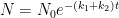
 latex N\rightleftharpoons B$
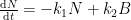

Described by the following differential equation:
having the following analytical solution:
This solution is not equivalent to a sum of exponentials of the form:
and is described by a system of differential equations of the form:
It is important to show the compartment box model if you are going to perform these calculations. This calculation assumes two parallel, irreversible processes:


Giving the following differential equation:
with the following analytical solution:
This solution is not equivalent to a sum of exponentials of the form:
consistent with the form given by the Bern Model.
Nor is it consistent with the compartment box model suggested by Gösta, which has the form:
yielding a system of differential equations of the form:
gymnosperm: “How good a proxy is 14CO2 for the other isotopes?”
My Paper 1 page 7 gives you a clue: “Carbon isotope effects encountered in
organic chemistry may occasionally be as high as 1.15 [16], but are normally much lower [17].
The kinetic isotope effects for events associated with the uptake of atmospheric carbon dioxide by
the hydrosphere or the biosphere have been extensively studied and are normally lower than 1.02 for C13 and 1.04 for C14 [18, 19].”
This means that the isotope effects are of negligible magnitude compared to the experimental error in data such as the bombtest curve. 14CO2 is an excellent proxy for CO2 in general and anthropogenic CO2 emissions in particular.
Dear Ferdinand Engelbeen,
Please forgive for saying so, but your meager knowledge of relaxation kinetics makes your comments so full of unjustified or erroneous statements that I had better confine myself to a few fundamental points that may help you understand why I disagree with most of your views on such topics.
1. F.E.: “residence time is how much CO2 is exchanged”
You accept the standard definition of residence/turnover time (used by the IPCC, used by me). What you may not realize is that this definition is a reformulation of the law of mass action; residence time is the reciprocal of the rate constant for a specified unidirectional output step and not a measure of exchange. Rate constants are system constants. Doubling the amount of CO2 does not change the corresponding residence time. All that happens is that the corresponding output rate is doubled.
And the “decay time” for 14CO2 is NOT a residence time. You seem to be the one of us who has a poor understanding of the difference between the two “time” concepts, i.e. the difference between rate constants and relaxation time constants (which are functions of the rate constants).
2. Almost all carbon cycle models are of multibox character and based on prescriptions of the law of mass action. The standard approach is to define the system by detailing the number of boxes considered, their interconnections, and the rate constants characterizing the exchange of carbon between the boxes. The law of mass action is then applied to express the relaxation kinetics (the pulse response) of the system in terms of differential equations such as d[CO2air]/dt = f(concentration variables; rate constants). To the extent that the equations have an analytical solution, they may prescribe that relaxations of concentration variables in the system are governed by exponential relationships. The solutions then also show how the corresponding relaxation times are related to rate constants in the system.
So, when you claim that a quantity “tau = Expression” represents the “excess mass decay rate” for CO2 emissions, you have to provide evidence for that claim. Define your system, show that the kinetic equations can be solved, show that the solution corresponds to exponential relaxation terms, and show that the relaxation time for CO2 is adequately described by your “Expression”. The latter seems unlikely, because relaxation times are functions of rate constants in the system and your “Expression” shows no obvious relationship to any rate constants at all.
3. F. E.: “Besides (negligibly small isotope effects), all carbon isotopes behave the same”
I agree, and the implication of your statement is that reaction schemes, rate constants, and the kinetic differential equations for all carbon isotopes are practically the same. Which means that solutions to the equations, and hence relaxation times, are practically the same for 14CO2 and emissions of fossil CO2. The possibility that the 14CO2 spike and emissions of fossil CO2 decay at widely different rates does not exist. Your claim that the latter relaxation time is 52.5 years is unsupported by tenable evidence and inconsistent with the relaxation time of 14 years empirically estimated for 14CO2 from the bombtest curve.
Bart says:
July 8, 2013 at 2:30 pm
Your interpretation runs completely afoul of the observed relationship
dCO2/dt = k*(T – Teq)
That is not the observed relationship, the observed relationship in your data fitting is:
dCO2/dt = k*T + offset
You assume that there is a Teq which is given by k*offset, you have no evidence for this.
There is no physically possible way to reconcile that observation with significant human forcing of atmospheric CO2.
Yes there is:
dCO2/dt = k*T + k1*CO2anthro +k2, where CO2anthro is the rate of human release of CO2.
“What is the effect of more CO2 on dCO2/dt.”
Negligible. That is what the relationship above shows.
No that’s a result of your assumption!
gostapetterson,
“The kinetic isotope effects for events associated with the uptake of atmospheric carbon dioxide by
the hydrosphere or the biosphere have been extensively studied and are normally lower than 1.02 for C13 and 1.04 for C14 [18, 19].”
Your source [19] is paywalled but I quote from [18]: “If stomatal diffusion is rapid (stomatal resistance is low) and carboxylation is limiting, the predicted isotope fractionation is 28%…If diffusion is slow (stomatal resistance is high), the predicted fracrionation is 4%…”
He is talking about C4 plants and C3 are a bit more efficient under dry (high resistance) conditions, but ocean biota don’t have this problem at all and moist tropical areas not so much.
Overall I would bet biological fractionation is closer to 1.1 than 1.02 for 13C and higher for 14C. I think you should give some serious consideration to heavy isotope concentration in the oceans where DIC just doesn’t care and 1/5 of the carbon cycle disappears every year into the abyss for a millennium.
Bart says:
July 8, 2013 at 3:46 pm
No circular reasoning. There simply is no such effect evident in the data.
Bart, if your formula (that is not data!) shows something that violates physics, then your formula is wrong.
If the CO2 pressure in the atmosphere increases, then the overall increase of CO2 into the atmosphere is decreased. Whatever the cause of the increase. That is independent of the type of process involved, as good for a static process as for a dynamic changing process.
ZP says:
July 8, 2013 at 7:09 pm
Thanks for the comment…
In my opinion, indeed the two processes involved are quasy independent of each other and both are practically irreversable.
The Bern model has its problems, and may be justified if you add most of all known reserves of oil and gas (at 3000 GtC) plus coal (at 5000 Gtc) to the atmosphere. Then several of the current fast sinks become saturated and even a “constant” fraction may be the case. Not with the up to current releases, which may give a 1% remaining fraction if all CO2 released equilibrates with the deep oceans (after several centuries).
Pettersson’s approach is that only the distribution of CO2 over the different reservoirs plays a role and doesn’t take into account the thinning caused by the deep oceans difference in 14C content.
In my opinion, both are wrong…
gostapettersson says:
July 8, 2013 at 8:29 pm
OK, I have some difficulties with the different (English) definitions, where several quite different ones are mangled for the same prcess and the same are used for quite different processes.
The possibility that the 14CO2 spike and emissions of fossil CO2 decay at widely different rates does not exist. Your claim that the latter relaxation time is 52.5 years is unsupported by tenable evidence and inconsistent with the relaxation time of 14 years empirically estimated for 14CO2 from the bombtest curve.
Again, what you forget is that the 14CO2 decay rate is heavily influenced by the “thinning” caused by the huge exchanges with deep ocean waters. What goes into the deep oceans is the current atmospheric composition, what comes out is the atmospheric composition of ~1000 years ago, minus the 14C decay rate. Anyway (far) lower than the post-bomb tests 14C level, 55% lower than the initial bomb spike.
That has nothing to do with the relaxation of any excess injection of CO2 in the atmosphere, which is more or less the same for all isotopes (except for the isotopic discrimination). That gives that the decay rate for 14C is much faster than for 12C.
The same happens for 13CO2:
http://www.ferdinand-engelbeen.be/klimaat/klim_img/deep_ocean_air_zero.jpg
Where only 1/3rd of the theoretical decay of 13C of the fossil fuel injection is found. Thus compared to the relaxation time of the extra CO2 injection, the relaxation of 13C vs. 12C is three times faster.
The 52.5 relaxation time is as empirical as your 14C relaxation time: based on real world changes in total atmospheric CO2 (as mass) vs. the extra pressure caused by the extra CO2 increase above the pre-industrial equilibrium. See the same explanation as mine by Dr. Peter Dietze in 1997:
http://www.john-daly.com/carbon.htm
It is a simple two box model where the extra amount (=pressure) invokes an extra outflow from one box (the atmosphere) into one other reservoir (representing all other reservoirs combined). Currently the extra outflow is 4-5 GtC/year for a level of 210 GtC (100 ppmv) above equilibrium, giving a relaxation time of over 50 years for the extra CO2 (all isotopes combined). Over 3 times slower than for 14C. Not by coincidence a similar upspeed as for 13C.
Phil. says:
July 8, 2013 at 9:02 pm
“You assume that there is a Teq which is given by k*offset, you have no evidence for this.”
Holy cow. Are you really this dense? I’ve tried to spoon feed it to you, but this is basic algebra. If you cannot understand it, give up. You have no hope of understanding anything about this system.
Ferdinand Engelbeen says:
July 9, 2013 at 12:08 am
“Bart, if your formula (that is not data!) shows something that violates physics, then your formula is wrong.”
No, it simply means that the effect is minor, and can be neglected. If you read through the comment above, you will see that I explain why.
Ferdinand Engelbeen says:
July 9, 2013 at 1:18 am
“What goes into the deep oceans is the current atmospheric composition, what comes out is the atmospheric composition of ~1000 years ago, minus the 14C decay rate.”
Just for the record, I agree with you here, and this is a singularly lucid explanation. There are undoubtedly several time constants involved, though the data indicate that those active in sequestering anthropogenic inputs are short.
It is also a window into the ocean pump. What was the composition of 1000 years ago? And, if it was much higher than today, how does that upwelling of higher content waters affect CO2 concentrations today? Answer: it produces a continuous pump into the atmosphere, which will not stop until the temperature/pressure/concentration states reach a new equilibrium.
Bart says:
July 9, 2013 at 9:11 am
Phil. says:
July 8, 2013 at 9:02 pm
“You assume that there is a Teq which is given by k*offset, you have no evidence for this.”
Holy cow. Are you really this dense? I’ve tried to spoon feed it to you, but this is basic algebra. If you cannot understand it, give up. You have no hope of understanding anything about this system.
It is clear that you don’t understand the system at all. You have asserted that the only explanation for the offset is Teq, however you have never attempted to justify this. Then in a classical case of circular reasoning you then assert that that means there is no role for human CO2 release! As I pointed out there could be other terms in that offset which you have not accounted for, including human CO2 release, which you blithely ignore. Explain why the offset must be completely accounted for by the Teq term and what evidence you rely on in that assertion. Mathematics without the proper physics/physical chemistry is meaningless!
ZP says:
July 8, 2013 at 7:14 pm
The actual set of ordinary differential equations is a truncated expansion in eigenmodes of the solution to a partial differential diffusion equation. They are generally a convenient fiction – until added together, they do not necessarily model actual, specific and discrete physical processes.
Each eigenstate has a specific time constant associated with it. When you add all the responses together, you get something like the Bern Model.
So, the problem with the Bern Model is not the methodology. It is that it has been fitted based on presumed dynamics which, it has now become evident, are wrong.
Phil. says:
July 9, 2013 at 9:53 am
I do not intend to waste any more time on you, Phil. You are so far out of your depth, it is just not worth the effort.
Bart says:
July 9, 2013 at 11:18 am
Phil. says:
July 9, 2013 at 9:53 am
I do not intend to waste any more time on you, Phil. You are so far out of your depth, it is just not worth the effort.
Bart you so tied up in your fake model and have no understanding of the underlying physics that I long ago gave up on your ever learning anything. The only reason for rebutting your nonsense is in case someone else here might think you know what you’re talking about. I suspect Ferdinand feels the same, other posters have said much the same, Steve Fitzpatrick for example.
You’ve not explained why this equation couldn’t equally explain the observations:
dCO2/dt = k*T + k1*CO2anthro +k2, just ran away and hid, as usual!
Phil. says:
July 9, 2013 at 12:47 pm
========================================
Yeah Phil, we’ve seen this before. Check out
http://wattsupwiththat.com/2013/01/20/analysis-shows-tidal-forcing-is-as-a-major-factor-in-enso-forcing/
and scroll to bottom. –AGF
I think the issue arises from the fact that Gösta is using formal kineticist’s terminology, while much of the climatology literature is written by scientists with (quite obviously) no formal training in kinetic analyses.
The simplistic waterbox model presented by Peter is identical to the kinetic model formulation presented by Gösta. The main difference is that Peter assumes three distinct decay periods. This assumption is inconsistent with the presented compartment box model and associated description, however. The more complex waterbox model can be summarized using the following reaction equations, where the reversible sinks (i.e. cycles) are combined into a single box to simplify the kinetic model:


irreversible addition processes:
reversible processes:
irreversible removal processes:
Let’s ignore the irreversible addition processes and accept the assumption that the remaining processes are governed by differential concentration levels. With these assumptions, the changes will be governed by the following system of differential equations:
While an analytical solution to this system of differential equations exists, it is fairly involved, so an abbreviated solution describing the CO2 atmospheric levels (A) is given as follows:
Notice: this solution is of the same form as that given by the Bern model.
The two coefficients (c1 and c2) are functions of:
1) the initial concentrations of CO2 in the atmosphere
2) the initial concentrations of CO2 in the reversible sinks
3) the individual rate constants governing the transfers into and out of each compartment.
The two lambdas are formally referred to as eigenvalues of the coefficient matrix. The eigenvalues are just functions of the rate constants, the values of which exist in the complex plane – (i.e. the numerical values for the eigenvalues need not be real numbers).
Since the rate constants are functions of temperature, the coefficients and eigenvalues will also be functions of temperature. However, only the rate constants obey the Arrhenius equation, so the coefficients and eigenvalues will vary in highly complex ways with changes in temperature. And, if the temperature changes with time, one cannot solve the system of differential equations analytically. The only option is to solve the system numerically.
Hopefully, this form will parse correctly:

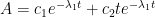
if the eigenvalues are not repeating:
otherwise:
Phil. says:
July 9, 2013 at 12:47 pm
“You’ve not explained why this equation couldn’t equally explain the observations”
Did, too.
Let us know when you’ve completed your first course in high school algebra. Then, maybe you can interact constructively.
agfosterjr says:
July 9, 2013 at 2:59 pm
Great. Tweedle-dee to the rescue of Tweedle-dum.
Gene Selkov says:
July 9, 2013 at 3:32 pm
Ah, another anti-Einstein crackpot. This thread has definitely jumped the shark.
Greg: “…comes close to reconciling Gosta Pettersson’s C14 curve and the Bern model”
Dear Greg, please be patient. I hope to be able to address other parts of your comments tomorrow, but today I will restrict myself to a simple technical question: The mathematical description of the bombtest curve.
As pointed out by Wallace you get a better fit the more exponential terms you add to your regression function. Ten exponential terms fit the curve better than a monoexponential function, but the fit is not much better. The descriptive rule you have to consider in such a case is to use the simplest function giving a satisfactory fit, i.e. a fit that is not improved with statistical significance when you add an extra exponential term. The decision as to the adequate number of terms to use can be made by standard statistical methods. Such tests formed the basis for my conclusions in Paper 1 that a monoexponential function provides a satisfactory fit and that no statistically significant improvement of fit was obtained for a biexponential function. Wallace seems to favour this view, as does the RMSE values he provides.
So, from a statistical point of view, the bombtest curve is best described as monoexponential. Otherwise, I wouldn’t mind a bit using Wallace’s biexponential function as an impulse response functionin my calculations. This would just confirm my conclusion that emissions only account for one half of the increased air level of CO2.
But I disagree with your statement that this reconciles the C14 curve and the Bern model. Relaxation times of the exponential terms in Wallace’s function seem to agree satisfactorily with those of the first two terms of the Bern model, but the amplitudes do not. Wallace’s function describes the observations made, the Bern model does not. Wallace’s function provides the same inferences as my monoexponential function, the Bern model provides entirely different inferences.
The reason for that is that the designers of model started by postulating what the inferences should be and then tuned parameter values in the model to be consistent with that postulate rather than with the observations made.
Bart says:
July 9, 2013 at 6:53 pm
Phil. says:
July 9, 2013 at 12:47 pm
“You’ve not explained why this equation couldn’t equally explain the observations”
Did, too.
No you didn’t come close to addressing it there.
Let us know when you’ve completed your first course in high school algebra. Then, maybe you can interact constructively.
Before you were born kid!
I do interact constructively, you on the other hand just get abusive with anyone who points out your lack of knowledge of the physics and doesn’t accept your bogus equation.
Ferdinand E.: “The main problem with the Pettersson 14C bomb spike is the dilution of 14C by the deep ocean and other reservoirs”
Phil: “14C diluted by CO2 from fossil fuel combustion, … also the oceans from which CO2 returns is depleted in 14C”
Greg: ” some correction to the C14 curve is required before the fitting”
Dilution effects on reported 14CO2/12CO2 ratios are approximately equal to (actually about 1% lower than) those indicated by the increased air level of CO2 during the examined periods of time; only an increase of atmospheric 12CO2 can dilute the atmospheric 14CO2/12CO2 ratio, and does so irrespective of whether the increase derives from fossil fuel combustion, return of 14C-free CO2 from the oceans, thermal outgassing, vulcanism or other sources.
Data in Fig. 2 of my Paper 1 have been corrected by consideration of the increased CO2 level (with the assumption that it exclusively derives from 12CO2). The correction, therefore, has taken care of all the dilution effects you discuss.
No additional corrections are required, unless you wish to correct the corrections for the fact that only 99% of the increase is 12CO2, the rest 13CO2. But such a sophisticated level of correction of the corrections is uncalled for because the corrections have a minor effect on the overall shape of the curve (the largest correction factor ≈1.2 applies for the latest point and raises its value from observed ≈4% to ≈5% in the corrected plot). The is borne out by my and Wallace’s regression analyses of the uncorrected data, which provide the same time constant estimate (≈14 years) as obtained for the corrected data.
gostapettersson says:
July 10, 2013 at 9:00 am
No additional corrections are required
Indeed, you did correct for the increase of CO2 in the atmosphere by the 14C free human emissions. But that is by far not the largest necessary correction.
The largest influence on 14CO2 levels is by the exchanges with the deep oceans: that is about 5% of all CO2 in the atmosphere which is replaced by deep ocean CO2. That doesn’t change the 12C levels of the atmosphere, but it does change the 14C level: what goes in the deep oceans is the current 14C/12C ratio, what comes out is the 14C/12C ratio of ~1000 years ago, minus the decay of 14C over that time frame.
Thus the problem is that you didn’t take into account the extra reduction of the 14C levels caused by the exchange with the deep oceans with 14C levels which are 55% lower than the peak bomb test values.
That gives the largest part of the 14 years relaxation time, not the redistribution of the extra CO2 in the atmosphere.
That makes that the relaxation time for the 14C spike is over 3 times faster than for the extra 12/13CO2 spike. And that you can’t assume that the 14C spike decay represents the fate of the extra CO2 spike…
Some addition:
only an increase of atmospheric 12CO2 can dilute the atmospheric 14CO2/12CO2 ratio
No, the exchange with the deep oceans doesn’t increase the 12CO2 mass in the atmosphere. It is only swapping amounts: the total amount of CO2 going in and out is near equal. But there is huge difference in 14C/12C ratio of what goes into the deep oceans and what comes out of the oceans. There is some 1000 years lag between sink and source. Thus anyway, what comes out the oceans is pre-bomb tests and what goes into the oceans is post-bomb tests…
Bart says:
> Ah, another anti-Einstein crackpot. This thread has definitely jumped the shark.
Heh. Those of us who are anti-nonsense don’t care about its origins. We don’t care if it comes from Einstein, Newton, our bosses, our girlfriends, or ourselves. When we see nonsense, we’re anti-everybody. No special treatment for you or your heroes — you’ll be greeted with the same crackpot attitude.
Ferdinand,

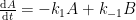

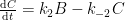


All physico-chemical processes are reversible. However, some processes are so slow as to be essentially irreversible. With that, you appear to be claiming that the reversibility of a 12CO2 molecule is substantially different from a 14CO2 molecule. If so (and quite frankly), the statement is incredible.
I’m assuming the the kinetic model that you are employing is best represented as follows (where A represents the atmospheric concentrations, B represents the upper ocean concentrations, and C represents the concentrations in the deep oceans).
(If this is incorrect, please provide the compartment box model – and associated system of differential equations – that you are assuming adequately describes the exchange process.)
This compartment box model will be governed by the following system of differential equations:
Your apparent assertion requires at least one of the following to be true:
1)
2)
3)
4)
Cases 1 and 3 are both inconsistent with known kinetic isotope effects; rate constants for heavier isotopes will be smaller than those of lighter isotopes. Thus, we can readily rule these two cases out. Cases 2 and 4 are also unlikely; the rate constants for 12CO2 should be a maximum of 5% larger than that for 14CO2.
Furthermore, the data provided by Gösta shows no apparent biphasic kinetic behavior implying that the loss of 14C follows (an/a set of parallel) irreversible pathway(s) or a single reversible pathway. The analysis by Gösta suggests the latter.
As the apparent claim is inconsistent with standard kinetic analyses, perhaps you have the data (or an alternative model) to support it. The required data would be the oceanic 14C concentrations as a function of time over the same time-frame as analyzed by Gösta. If plausible, we would expect the concentrations in the upper ocean layers to grow with time before decaying as the 14C flows into the deep ocean layers. The 14C concentrations in the deep ocean should grow slowly with time, followed by a more rapid growth and finishing with a slow growth rate. If you do not have these data, then Gösta’s analysis is significantly more plausible and consistent with standard kinetic analyses which invoke Occam’s razor.
Phil: “C14 decay curve isn’t representative of CO2 because it’s the result of a different set of
sources and sinks. C14 is created in the atmosphere from nitrogen”
Sources and sinks are of no primary interest as concerns representativity. Anthropogenic CO2 emissions come from many different sources, and sinks for 14CO2 and anthropogenic CO2 are the same (the hydrosphere and the biosphere).
The 14CO2 spike was created from nitrogen by the bomb tests, but once created it decays by the same reactions and mechanisms as CO2 in general. The C14 decay curve is representative of CO2 fro the simple reason that 14CO2 is carbon dioxide and carbon isotope effects are of negligible magnitude.
Assuming the systems response to C12 is the same as it is to C14, we can model the behaviour using control theory. We already know the Step Response (from the bomb tests).
ZP says:
July 10, 2013 at 5:35 pm
With that, you appear to be claiming that the reversibility of a 12CO2 molecule is substantially different from a 14CO2 molecule
Not at all: for the decay of any excess CO2 in the atmosphere, 12CO2 and 14CO2 follows the same rules, besides some small differentiation from isotope kinetics.
But for exchanges with the deep oceans, there is (near) zero decay for 12C, but a huge decay rate for 14C due to differences in 14C/12C ratio between what is in the atmosphere and what returns from the oceans.
I’m assuming the the kinetic model that you are employing is best represented as follows
In general it is simpler, as the deep ocean exchanges largely bypass the ocean surface, as well as at the sink places (mainly NE Atlantic) as at the source places (mainly near the Chilean coast).
If plausible, we would expect the concentrations in the upper ocean layers to grow with time before decaying as the 14C flows into the deep ocean layers.
See: http://shadow.eas.gatech.edu/~kcobb/isochem/lectures/lecture10_14C.ppt
From sheet 13 on, the 14C bomb spike in the oceans is covered.
Of particular interest is sheet 17, where the 14C spike (of +1000 per mil in the atmosphere) is largely suppressed at the Galapagos islands, due to the nearby deep ocean upwelling near the Chilean coast.
The deep ocean exchanges don’t influence the 12CO2 levels in the atmosphere, except for the difference between the inputs an outputs (which for the deep oceans currently is estimated at 2 GtC/year). But it does influence the 14C/12C ratio, even if there was no difference between inputs and outputs, as what comes in has a (much) lower 14C/12C ratio than the ratio in the atmosphere.
That makes that the decay rate of the 14C/12C ratio quite differs from the excess CO2 decay rate in general.
For excess CO2 decay (all isotopes) the formula is:
dCO2/dt = -k1*(C – Ceq)
where C is the current CO2 level (~400 ppmv) in the atmosphere and Ceq the equilibrium CO2 level for the current temperature (~290 ppmv).
Specific for 14CO2 the formula is:
dCO2/dt = -k1*(C14 – C14eq) – k2*(C14 – C14aq)
Where C14 is the current 14CO2 level in the atmosphere, C14eq the equilibrium 14CO2 level at the current temperature (quite similar to the general CO2 decay) and C14aq the 14CO2 level which returns from the deep oceans.
In this case k2 >> k1. The 14CO2 bomb spike relaxation is mainly by thinning of the concentration by deep ocean exchanges, not from the excess CO2 decay.
justjoshin says:
July 10, 2013 at 7:19 pm
Assuming the systems response to C12 is the same as it is to C14, we can model the behaviour using control theory. We already know the Step Response (from the bomb tests).
See my response to ZP: the system response to 14C is the same as for 12C for mass transfer, but additionally 14C is also removed by concentration differences between what returns from the deep oceans and what is present in the atmosphere…
gostapettersson says:
July 10, 2013 at 6:13 pm
The C14 decay curve is representative of CO2 fro the simple reason that 14CO2 is carbon dioxide and carbon isotope effects are of negligible magnitude.
That is true for the mass transfers which in general are the same for all isotopes, but for 14CO2 there is an extra concentration transfer which isn’t present for 12CO2 and which is much larger than for the mass transfers. Thus the 14C decay curve is not representative for the CO2 mass transfers…
gostapettersson says:
July 10, 2013 at 6:13 pm
Phil: “C14 decay curve isn’t representative of CO2 because it’s the result of a different set of
sources and sinks. C14 is created in the atmosphere from nitrogen”
Sources and sinks are of no primary interest as concerns representativity. Anthropogenic CO2 emissions come from many different sources, and sinks for 14CO2 and anthropogenic CO2 are the same (the hydrosphere and the biosphere).
The 14CO2 spike was created from nitrogen by the bomb tests, but once created it decays by the same reactions and mechanisms as CO2 in general. The C14 decay curve is representative of CO2 fro the simple reason that 14CO2 is carbon dioxide and carbon isotope effects are of negligible magnitude.
No they aren’t since the CO2 at the ocean surface is order 1,000 years old which doesn’t effect C12 but certainly does deplete the C14 returning from the ocean surface.
The equation that you have provided does not support your description. The equation you provided states that 14C will reversibly pass directly into the deep ocean without any exchange with the surface waters. And, will also reversibly exchange between the surface and atmosphere. So, the suggested model is correctly described by the following compartment box model:

As before A represents the atmospheric concentrations, B is the fast, reversible equilibrium (your C14eq term) and C represents the the deep ocean (your C14aq) term.
The solution to this system will again be consistent with the Bern Model with two terms. As stated previously, the solution will have two eigenvalues, the values of which will be functions of the rate constants.
Unless the equilibration with the biosphere is virtually instantaneous, this model would predict biphasic kinetics for the atmospheric 14C concentrations. This is not observed in the data.
Thanks for the data, but it does not provide justification for employing an mathematical model that is not founded in the language of formal kinetics. I strongly recommend that you revisit your thinking on this subject. Draw out the process using compartment boxes to represent the various sources and sinks. Draw arrows (reversible or not) from each source to each sink. From this diagram, write out the formal differential equations describing the process. Decide if a solution exists and solve the system either analytically or numerically, as applicable.
ZP says:
July 11, 2013 at 6:18 am
Ferdinand Engelbeen says:
July 11, 2013 at 3:15 am
In general it is simpler, as the deep ocean exchanges largely bypass the ocean surface, as well as at the sink places (mainly NE Atlantic) as at the source places (mainly near the Chilean coast).
Specific for 14CO2 the formula is:
dCO2/dt = -k1*(C14 – C14eq) – k2*(C14 – C14aq)
Where C14 is the current 14CO2 level in the atmosphere, C14eq
The equation that you have provided does not support your description. The equation you provided states that 14C will reversibly pass directly into the deep ocean without any exchange with the surface waters. And, will also reversibly exchange between the surface and atmosphere. So, the suggested model is correctly described by the following compartment box model:
No that isn’t a correct model, you have omitted the irreversible decay in reservoir C!
ZP says:
July 11, 2013 at 6:18 am
The equation you provided states that 14C will reversibly pass directly into the deep ocean without any exchange with the surface waters.
The deep ocean exchanges indeed largely bypass the surface, but are virtually non-reversable, as what returns from the deep oceans is what was going down some 1000 years ago. Thus the excess 14C in the atmosphere will be gone long before some of it returns from the deep oceans, and even that effect will be diluted, as smeared with a long period (several hundred years) filter. The C14aq in practice may be used as a constant.
The removal of total CO2 (including 14CO2) in excess as mass is quite fast distributed over ocean surface and vegetation with relaxation times of around 1 year, thus near instantaneous, but limited in quantity (10% of the change in the atmosphere for ocean surface). The more permanent storage in vegetation and deep oceans is what takes much more time.
Further, the 14C dilution is the result of two quite different processes: the general process of removal of an excess amount of CO2, which is mainly pressure (difference) related and the specific process of 14C concentrations changes by deep ocean exchanges which is mainly temperature (difference) related. These processes are virtually independent of each other and simply work in parallel.
As the exchange with the deep oceans is about a factor 20 larger than the removal rate of the excess amount of CO2 (all isotopes) into the deep oceans, it is no wonder that the excess removal rate has hardly any effect on the decay rate of 14CO2. Even the inclusion or exclusion of the thinning of 14C by the use of 14C-free fossil fuels at twice the excess removal rate had little effect (less than 1%) on the decay rate of 14CO2.
That may or may not match the different terms of the Bern model, but that is not the base of my reasoning. The base is that the empirical findings show a relaxation time for 14CO2 of ~14 years, while the relaxation time for the extra CO2 injection is ~52 years, over three times slower.
Similar as for the relaxation time of the 13CO2 depleted CO2 from fossil fuel burning: 3 times faster for 13CO2 than for the bulk of CO2, thanks to the deep ocean exchanges:
http://www.ferdinand-engelbeen.be/klimaat/klim_img/deep_ocean_air_zero.jpg
But if you want, I can try to make a multi-box model with all exchanges on it…
Phil. says:
July 11, 2013 at 6:45 am
No that isn’t a correct model, you have omitted the irreversible decay in reservoir C!
Look at it again. Irreversible decay is simply governed by the magnitude of k2 as compared to k-2. All processes are reversible in accordance with the principle of microscopic reversibility. However, some processes take a long time to reverse due to differences in magnitudes of the rate constants.
Clarification, some processes appear to be irreversible due to large differences in the magnitudes of the rate constants.
ZP says:
July 11, 2013 at 8:29 am
Phil. says:
July 11, 2013 at 6:45 am
No that isn’t a correct model, you have omitted the irreversible decay in reservoir C!
Look at it again. Irreversible decay is simply governed by the magnitude of k2 as compared to k-2. All processes are reversible in accordance with the principle of microscopic reversibility. However, some processes take a long time to reverse due to differences in magnitudes of the rate constants.
No, that refers to rate of transfer to and from the deep, during the ~1,000 years the C14 spends in the deep it decays to N14, that is not a reversible process! In fact by measuring the C14 at the ocean surface is how we know that the surface water is ~1,000 years old. You can find the data at: http://radiocarbon.pa.qub.ac.uk/marine/
Rather than show the deep water interaction as a reversible reaction you should show it as three sequential reactions, the C14 that returns from the deep has decayed, your model doesn’t include that.
Yes… please. Only after having the compartment-box model can we begin interpreting the observations using formal kinetics. And, of course, compare/contrast the other models presented.
Just to clarify… It’s not my model… I haven’t provided any… I’ve just been trying to understand the model assertions (given by Ferdinand) in terms of standard kinetic analyses.
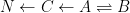
If you want to include a 14C decay pathway… fine. It will make the compartment box model more descriptive and (perhaps) complete. I assume you only want the pathway to be associated with loss from the “deep ocean” box? I’ll also make the loss to the deep ocean “irreversible.” The model now reads:
This modification doesn’t change anything, however. This model will predict biphasic kinetic behavior unless the equilibriation process is virtually instantaneous relative to the irreversible pathway.
Z. P.: “The solution to this system will again be consistent with the Bern model with two terms”
I guess you mean that the solution is consistent with a Bern model type of impulse response function with multiple exponential terms. But since your statement might be interpreted to provide support for the Bern model, I would like to add that a system containing N boxes will give rise to an impulse response function containing N-1 exponential terms. The simple two-box model in my Paper 3 gives one exponential term, your three-box model gives two terms, and so forth. The more complex you make your system, the more exponential terms the solution defines. To the extent that the kinetic differential equations can be analytically solved.
The Bern model is so complex that no analytical solution can be found. Its impulse response function has been determined pragmatically by modelling what happens when you add a pulse of CO2, followed by fitting a multiexponential regression function to the model results. There is nothing wrong with that approach or with their use of an impulse response function containing several exponential terms. The problem with the model is that it does not describe what it is claimed to describe.
Ferdinand Engelbeen,
Thank you for providing us with the kinetic equations for the (two-box) model you use to illustrate what you mean. This makes it easy to pinpoint where you have gone wrong in your analysis.
1. You cannot change the examined system to get an argument. If you assume that excess CO2 decay (all isotopes) is irreversible, i.e. dCO2/dt = -k1*(C-Ceq), then you have to assume that the same applies for 14CO2. You get the same differential equation for both species, and the same solution stating that the decay will be exponential with a relaxation time given by 1/k1.
If you use the reversible type of formula for 14CO2, you should do so too for CO2, in which case the solution still will be the same for both species and prescribe that the relaxation time is given by 1/(k1+k2).
2. Your main argument seems to be based on the reversible case and the belief that k2>>k1. For the two-box system your formulas describe, k2 and k1 are interrelated through k2/k1=Keq, where Keq≈0.02 according to the IPCC carbon cycle data. So, you do NOT have k2>>k1. On the contrary, k2 is more than 50 times smaller than k1 !!! That’s why the oceans contain some 60 times more carbon than the atmosphere. That’s also why the relaxation time for CO2 comes close to that for the irreversible case: 1/(k1+k2)≈1/k1
Trust me, events in the deep ocean cannot change these consequences of the strong irreversibility of the transfer of CO2 from the atmosphere to the hydrosphere. On second thought, don’t trust me but convince yourself that such is the case by following the advice given by Z. P.: Define a three-box system (air-surface sea-deep sea), set up the kinetic diff. equations and solve them. But take care to ensure that the overall equilibrium properties of the system are consistent with the available empirical equilibrium data. The Bern model designers did not.
gostapettersson says:
July 11, 2013 at 9:12 pm
1. You cannot change the examined system to get an argument. If you assume that excess CO2 decay (all isotopes) is irreversible, i.e. dCO2/dt = -k1*(C-Ceq), then you have to assume that the same applies for 14CO2.
Agreed, but that is only for the common part of decay: the decay of the amount that is in excess.
Your main argument seems to be based on the reversible case and the belief that k2>>k1
As wel as for k2 as for k1 the reactions are practically irreversible and still k2>>k1. The difference between the two is that the second reaction only affects 14CO2 (and 13CO2) and doesn’t affect 12CO2. Ultimately all will approach equilibrium, but 14CO2 and 13CO2 will approach it (about three times) faster than 12CO2.
The reason is that the return from the deep oceans is largely disconnected (~1000 years) from what goes into the oceans. That means that what returns from the oceans has a much lower 14C/12C ratio (and a much higher 13C/12C ratio) than what goes into the oceans: 50% lower than the bomb spike, 55% if you include the radioactive decay.
There is also the matter of quantities involved:
– the result of the 100 ppmv (210 GtC) excess CO2 in the atmosphere is a net loss of 4-5 GtC/year. 1 GtC/yr goes into vegetation (as calculated from the oxygen balace). 0.5 GtC goes into the ocean surface (as calculated from the buffer factor), the rest, 2-3.5 GtC/year in the deep oceans.
– the result of the ~40 GtC/yr exchanges between deep oceans and atmosphere thus returns 5%-9% less CO2 mass (mainly 12CO2) than was absorbed. But it returns 55% less 14CO2 than was absorbed in the first year of the bomb spike…
ZP says:
July 11, 2013 at 3:30 pm
This modification doesn’t change anything, however. This model will predict biphasic kinetic behavior unless the equilibriation process is virtually instantaneous relative to the irreversible pathway.
If we may assume that both processes are practically irreversible, only with different decay times (and largely towards the same reservoir…), why should that give a biphasic behavior? Isn’t the combination acting as if it were a single sink with a shorter decay time, as Gene Selkov said: the harmonic mean of the two processes…
Ferdinand Engelbeen: “As well as for k2 as for k1 the reactions are practically irreversible and still k2>>k1”
A practically irreversible reaction by definition is characterized by k2<<k1, as the rate constants are defined by your formulas.
I am sorry to say that you have too much to learn about reaction kinetics already at the most elementary level (rate and equilibrium constants) to be able to understand the kinetic evidence presented in my paper, or to be able to present any tenable kinetic arguments regarding that evidence.
There in lies the problem… we can’t treat (mathematically) an equilibrium process as if it were irreversible. Formally, rate laws are statements of how a system evolves as it strives to reach thermodynamic equilibrium. As Gösta stated, the ratio of the forward to reverse rate constants is the equilibrium constant for the process. If we treat an equilibrium process as irreversible, we are making a strong statement that we believe the magnitude of the equilibrium constant is so large that the process essentially goes to completion.


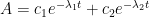


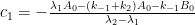
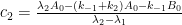
To understand why this is the case, consider the following. Equilibrium is defined as the state where the forward rate is equal to the reverse rate (commonly referred to as the dynamic equilibrium). Therefore, for the following process:
Equilibrium will reached when the time derivative of the concentration of A is zero:
such that:
Thus, the ratio of the forward to reverse rate constants must conform to the known equilibrium constant for the system (e.g. Henry’s law constant).
Things get a quite a bit more mathematically complex when we introduce another pathway (box). What happens in these cases is we get coupling between the processes. Consider the reversible, consecutive system:
The time derivative of the concentration of A depends on both the concentration of A and the concentration of B. However, in the case of B, the time derivative depends on the rate of production (from A) and loss by two pathways (reversibly to A and irreversibly to C). Essentially, the A to B system is striving to reach equilibrium while B is being slowly siphoned off to produce C. This “tug-of-war” on B is what leads to the observed biphasic kinetic behavior of A. The concentration of A will initially drop quickly as equilibrium is being established. Once equilibrium with B has been established, the continued loss of A will be at the same rate that B is converted into C. Hence, two distinct decay regimes.
Having the solution to the system of differential equations will really aid in fully grasping these concepts. With the solution, you can play with values of the rate constants and see how the system behaves. You’ll also be able to see the extreme cases such as when k1 >> k-1, which leads to the situation where the system is adequately described as consecutive, irreversible processes:
or the other extreme, where k2 << k-1 such that the second process is essentially irrelevant to understanding the concentration vs. time profile for A.
For the reversible, consecutive system, the following differential equations are:
The analytical solution to this system (apologies in advance if I made an algebra and/or transcription error) is given as follows:
where the two eigenvalues are:
and the two coefficients are:
Here is a nice resource to look at:
http://voh.chem.ucla.edu/vohtar/spring05/classes/156/pdf/COMPLEX%20REACTIONS_2005_2.pdf
On pages 9 & 10, the author provides this system with an example of the biphasic kinetic plot. And on page 12, the author provides the complete solution assuming B0 = 0 and the second step is reversible.
Another nice resource is found here:
http://nova-transnet.com/zonanova/downloads/documentos/Basic%20Pharmacokinetics.pdf
The author provides concrete examples of how to use Laplace transforms to solve the compartment box models starting in section 2-44.
Ferdinand,
I would love to see your model. I’ve been trying to figure out how to do it putting formula windows in the NOAA or GFDL Carbon cycle graphics. Also very interested in how to approximate ocean chemistry from two or three of the variables.
gostapettersson says:
July 12, 2013 at 6:09 pm
A practically irreversible reaction by definition is characterized by k2 much smaller than k1, as the rate constants are defined by your formulas.
What you seems to refuse to understand is that both decay processes for 14C are (near) completely independent of each other. Thus k2 and k1 have not the slightest connection with each other. They simply work in parallel. Both are decay rates, not return rates (should have supplied them too as k-1 and k-2). k1 maybe much larger than k2 or reverse, in practice it is k2 which leads k1.
The general decay of all CO2 (all isotopes alike) is caused by pressure differences between atmosphere and oceans (both surface and deep oceans) and the biosphere. That is the first decay rate, which is bidirectional, but as the deep oceans are much larger in carbon content, in practice irreversible.
The specific decay for 14CO2 (and 13CO2) is caused by the concentration differences of what goes in and out other reservoirs. That is not much different for vegetation and the ocean’s surface, but is quite different for the deep oceans. That is the second decay rate, which is bidirectional, but as the deep oceans are much larger in carbon content, in practice irreversible. The second decay rate is only applicable to 14CO2 (and 13CO2), not to 12CO2.
Even if exactly the same quantities of total CO2 come back from the deep oceans as which did go in, what comes out as 14CO2 concentration is less than halve the concentration of what did go in at the peak of the bomb spike. Thus only halve the quantity of 14CO2 returns in the first year bomb spike than what did go in, while (near) exactly the same amount of 12CO2 returns (minus the negligible difference in 13CO2 and 14CO2 mass).
I am sorry to say that you have too much to learn about reaction kinetics already at the most elementary level
After 34 years practical experience with chemical processes by correcting theoretical models which didn’t work in reality (and 8 years of enjoyed retirement), I have forgotten most of the theoretical side, but still know where to look for the practical pitfalls of the theories…
ZP says:
July 12, 2013 at 6:34 pm
Should learn Latif, but have finished the process flows, I made two flowcharts with realistic figures for the years 1960:
http://www.ferdinand-engelbeen.be/klimaat/klim_img/14co2_distri_1960.jpg
and for 2000:
http://www.ferdinand-engelbeen.be/klimaat/klim_img/14co2_distri_2000.jpg
Here some more background (I hope that makes it clear):
The main process of redistribution of an excess CO2 injection is the same for all isotopes.
There are three main reservoirs where the excess CO2 can get into in reasonable time:
– vegetation
– ocean surface
– deep oceans.
The huge exchanges back and forth between air and vegetation/ocean surface and the limited uptake of both (10% of the change in the atmosphere for the ocean surface, 0.5% in vegetation) makes that the decay rates are quite fast (5 years according to the IPCC, 2 years to regain equilibrium of in/outflows).
The main process of redistribution of an excess 14CO2 follows the same rules as for all isotopes. Except that for the deep oceans there is an extra process at work: the concentration of what goes into the oceans largely differs from what comes out.
That is an (near) entirely separate process than the redistribution of all CO2 together. Thus to make the basis complete (where the = sign means the reversible reactions) for A (atmosphere), B (deep oceans), C(ocean surface) and D (biosphere):
A = B
A14 = B14
A = C
A14 = C14
A = D
A14 = D14
For simplicity, you may forget the ocean surface and vegetation out of the equations and simply add the redistribution to the deep oceans (where the bulk of the increase ultimately will reside). Both are fast in equilibrium for all isotopes and have little contribution to the mass decay. Over the period 1960-2000 the overall mass increase of vegetation was near zero
.
Thus for the current discussion forget all C&D reactions as well as for total CO2 as for 14CO2. What is left is the sink and source rates between atmosphere and deep oceans, for total CO2 and 14CO2.
Pre-bomb 14CO2 in the atmosphere and other reservoirs was ~50% of the bomb peak strength, more or less in equilibrium. Cosmic rays then supplied about 6% per year, which compensated for the losses in other reservoirs (mainly the oceans).
Thank you for the flowcharts. These diagrams make it clear that your model would predict a multiphasic decay profile for 14C from the atmosphere.
Ferdinand,
Very impressive flow charts.
ZP says:
July 13, 2013 at 5:35 am
These diagrams make it clear that your model would predict a multiphasic decay profile for 14C from the atmosphere.
As most of the distribution of the extra 14CO2 bomb releases into the ocean surface and the biosphere already occured before the peak value was reached and there is hardly any further decay in these reservoirs, I don’t see how that would be observable in the (relative) huge decay caused by the return of low 14C out of the deep oceans.
Thus my question is: what happens with 14CO2 compared to 12CO2 with the two decay rates involved for the deep oceans only: the in/out mass difference (for both) and the in/out concentration difference (for 14CO2 only)?
gymnosperm says:
July 13, 2013 at 10:43 am
Very impressive flow charts.
Thanks, the mass transfers are from GISS, but backcalculated for the 1960 data from the Mauna Loa curve and the known human emissions. The distribution in the ocean surface is based on the Revelle factor (for 12CO2 and 14CO2 alike). The distribution in the biosphere is from Battle e.a. where vegetation was a small net emitter before 1990 and a small, but increasing absorber after 1990.
The main uncertainty is the isotopic behaviour for vegetation and the ocean surface. At one side, when the concentration in the atmosphere drops (into the deep oceans), then the higher concentrations in vegetation and ocean surface will give some of it back to the atmosphere. On the other side, some of it drops out into the deep oceans (mainly as organics) or gets into more permanent land storage (humus, peat, browncoal,…).
So this are the basic isotopic schemes, open to improvements…
gymnosperm says:
July 13, 2013 at 10:43 am
“Very impressive flow charts.”
But, basically a balancing of the books according to a specific, and non-unique, scenario. I has no probative value.
It has no probative value.
Let’s ignore what happened before the peak value occurred as it won’t change the mathematical analysis. We can accurately analyze the implications of the proposed model without loss of information.


In short, you are showing three coupled equilibria as follows:
In this case, the observed time decay profile of 14C from the atmosphere levels will be dependent on the transfer rates into and out of each of the three sinks. So far, so good?
However, you appear to be asserting a critical mathematical constraint that equilibrium of the atmosphere with the surface and biosphere had been established by the time we started our analysis (i.e. at the peak value). If so, the rates into and out of those sinks must be equal by definition of equilibrium. Thus, the loss of A would be controlled only by the equilibration rate with the deep oceans.
However, this criterion is contrary to your flow diagram that appears to show the mass transfer rates into and out of the ocean surface and biosphere sinks as being unequal (i.e. there is a small net positive transfer into the sinks). Therefore, those systems are not at equilibrium (again by definition). The transfer rates into and out of a sink must be equal at all times in order for those sinks to be in equilibrium. If the sinks are not in equilibrium, then the model will predict a multiphasic kinetic profile for the loss of 14CO2 from the atmosphere. If the sinks are in equlibrium, then the model collapses to just:
which is indistinguishable from the model given by Gösta, albeit the interpretation of the parameters are slightly different.
ZP says:
July 13, 2013 at 1:52 pm
which is indistinguishable from the model given by Gösta, albeit the interpretation of the parameters are slightly different.
Except that the decay rates for 12CO2 (the bulk) and 14CO2 are widely different:
– in 1960, the mass loss of 12CO2 from the atmosphere into the deep oceans is:
(40-41) GtC/690 GtC = – 0.15%
– in 1960, the mass loss of 14CO2 from the atmosphere into the deep oceans is:
(( 40 GtC * 45% ) – (41 GtC * 100%)) / (690 GtC * 100%) = -3.33%
– in 2000, the mass loss of 12CO2 from the atmosphere into the deep oceans is:
(40-41.7) GtC/780 GtC = -0.22%
– in 2000, the mass loss of 14CO2 from the atmosphere into the deep oceans is:
(( 40 GtC * 45% ) – (41.7 GtC * 60%)) / (780 GtC * 60%) = -1.5%
In 1960, the 12CO2 level in the atmosphere was 17% above equilibrium
In 1960, the 14CO2 level in the atmosphere was 100% above equilibrium
In 2000, the 12CO2 level in the atmosphere was 28% above equilibrium
In 2000, the 14CO2 level in the atmosphere was 20% above equilibrium
For the same % above equilibrium, one should expect the same % mass loss, if a similar process with the same decay rate is at work.
In this case, different processes are at work: the decay of an excess amount 12CO2 in the atmosphere only depends on the difference between inputs and outputs (which is pessure dependent), while the decay rate of the 14CO2 bomb spike additionally depends on the bulk of the exchanges rates (which is temperature dependent) and the concentration differences between inputs and outputs.
Thus while the model is similar, the decay rate of 14CO2 is much faster than the decay rate of 12CO2, which represents near 99% of all CO2. And thus is the 14CO2 bomb spike curve not representative for the decay of an extra injection of CO2 above equilibrium.
It doesn’t matter. The predicted behavior is a direct consequence of the axioms of mathematics.
ZP says:
July 13, 2013 at 3:39 pm
It doesn’t matter. The predicted behavior is a direct consequence of the axioms of mathematics.
Agreed.
But the theory of Gösta Pettersson was:
the bombtest curve can be taken to be representative for the relaxation of emission pulses of carbon dioxide in general.
is proven false as different relaxation times are involved…
Bart says:
July 13, 2013 at 1:32 pm
But, basically a balancing of the books according to a specific, and non-unique, scenario. I has no probative value.
Besides balancing the books based on relative constant exchange rates between the different compartiments, the 14CO2 decay proves that there is no increase in exchange rates with the deep oceans over the period 1960-2000.
Human emissions increased a 2.8 fold 1960-2000.
If natural turnover is responsible for the atmospheric increase, the total natural inflows must have increased in ratio: from 180 GtC/year to 500 GtC/yr, assuming the estimates of 1960 as start.
As vegetation and ocean surface turnover are limited in variability, the deep oceans must take the difference, thus + 320 GtC/year turnover. That gives following flow estimates for the year 2000:
http://www.ferdinand-engelbeen.be/klimaat/klim_img/14co2_distri_2000_2.jpg
That doesn’t give a difference in net mass distribution, but it gives a huge difference in 14CO2 distribution:
With the extended deep ocean turnover in 2000, the mass loss of 14CO2 from the atmosphere into the deep oceans in one year then is:
(( 360 GtC * 45% ) – (361.7 GtC * 60%)) / (780 GtC * 60%) = -11.8%
Thus if there was such a real increase of natural deep ocean – atmosphere turnover, the year 2000 drop of 14CO2 from the bomb tests would be below the pre-bomb tests value, in only one year… Which isn’t observed.
The increase of deep ocean turnover thus is proven false (as good as it was from the 13CO2 decay rate).
This statement requires proof through calculation of the rate constants. Guesstimation of annual fluxes is not proof nor are assertions that the kinetic isotope effect will be unusually large for this system. At this time, I fail to see how your claim is defensible.
ZP says:
July 14, 2013 at 8:02 am
Guesstimation of annual fluxes is not proof nor are assertions that the kinetic isotope effect will be unusually large for this system.
The difference in rate constants is not caused by kinetic isotope effects, it is caused by a combination of sink rate (which is nearly the same for all isotopes) and the difference in concentration between 14C (or 13C) and 12C for what goes into the deep oceans and what comes out.
The observed relaxation time for an excess CO2 injection is 51.5 years.
The observed relaxation time for an excess 14CO2 injection is 14 years.
For 12C that is the effect of C – Ceq only.
For 14C that is the combined effect of C – Ceq ánd 14C – 14Caq.
Where the effect of the combination on 14C decay is much larger than the single effect on 12C.
Rate constants are independent of concentrations by definition. The rate of a non-zero-order process, however, is dependent on concentrations (as well as the rate constant).
ZP says:
July 14, 2013 at 1:38 pm
Rate constants are independent of concentrations by definition.
You need to take into account the huge lag of ~1000 years in the deep oceans between sink and source.
In this case the difference in concentration influences the relative quantities of 14CO2 vs. 12CO2 of what returns from the deep oceans.
What goes into the deep oceans has the composition of today’s atmosphere.
What comes out has the composition of the atmosphere of ~1000 years ago.
What comes out of the oceans contains 97.5% of the 12CO2 quantity compared to what was absorbed, in 1960 (96% in 2000).
What comes out of the oceans contains 97.5%*0.45 = 44% of the 14CO2 quantity compared to what was absorbed in 1960, the year of the 14CO2 bomb test peak (96%*0.75 = 72% in 2000).
Same process, largely different rate constants.
Ferdinand,
We do not observe relaxation times. For simple processes, we can infer the value directly from a concentration vs. time plot. For complex processes, we must calculate a relaxation time from the values of the rate constants.
The model you keep asserting predicts a biphasic decay profile. The model and associated arguments are simply mathematically untenable.
“It doesn’t matter. The predicted behavior is a direct consequence of the axioms of mathematics.”
Too funny, as if we knew what the applicable axioms of mathematics were. In order to adequately describe the system mathematically, you must be able to describe it in language. Language and mathematics are both metaphor, they are both models. We have been telling the climate “scientists” for years that we are working with a system with third and fourth and who knows how much higher order differentials.
You understand the system, THEN you apply the mathematics. Well, backing off a couple steps, you can test the system with mathematical models, but when they fail, you have to be willing to throw them out.
ZP says:
July 14, 2013 at 3:49 pm
We do not observe relaxation times. For simple processes, we can infer the value directly from a concentration vs. time plot. For complex processes, we must calculate a relaxation time from the values of the rate constants.
May I respectfully disagree? There are a lot of natural processes which can’t be described in mathematical terms (as Gymnosperm already said), like the relation between CO2 levels in the atmosphere and temperature. That is the result of hundreds of independent and interdependent processes, of which several are far from linear. Despite that, the overall dependence of CO2 on temperature is near linear, where much of the deviation is from different lag times for CO2, not from a change in ratio:
http://www.ferdinand-engelbeen.be/klimaat/klim_img/Vostok_trends.gif
Thus for all practical purposes, one can use the 8 ppmv/°C ratio.
The same for the 14CO2 bomb curve, which is the result of several decay rates: the redistribution of the extra CO2 injection in the atmosphere (as mass) into other reservoirs and the specific decay of 14CO2 due to thinning from the 14CO2-free human emissions and the specific decay of 14CO2 due to the long lag in the deep oceans.
For all practical purposes, the observed relaxation time of 14 year can be used, as that shows a quite simple linear behaviour…
For the bulk of CO2 (which is near 99% 12CO2), the observed relaxation time is over 50 years, only as result of the redistribution over the different reservoirs, again showing a quite simple linear behaviour.
In addition, the linearity of the increase in the atmosphere and the net sink rate shown here via the accumulated human emissions:
http://www.ferdinand-engelbeen.be/klimaat/klim_img/acc_co2_1960_2006.jpg
The sink rate is the difference between human emissions and the increase in the atmosphere, thus also linear, whatever other processes are involved…
I am only referring to the proposed compartment box model.
For small changes in x, all functions can be approximated as linear. However, this does not imply that the behavior is linear for all x. In the case of the temperature dependence of the solubility of CO2 in water, the observed behavior conforms to the van’t Hoff equation.
I suppose you are referring to the half-life of a first-order decay, where the half-life is a constant. Otherwise, you appear to now be suggesting that the decay rate should be of zero-order.
These claims are simply not tenable. Either the rate laws describing the changes in CO2 are dependent on concentration (or pressure) differences, or the rate laws are of of zero-order. The rate laws cannot be both. If the rate laws are of zero order, then the observed loss of 14C would be adequately described by a linear equation. Otherwise, your only option is to model the system using a compartment box model and properly formulated differential equations.
ZP says:
July 15, 2013 at 5:49 am
In the case of the temperature dependence of the solubility of CO2 in water, the observed behavior conforms to the van’t Hoff equation.
Indeed, non-linear. That makes it very remarkable that the increase of CO2 in the atmosphere is with a near fixed ratio to temperature over a large range (190-290 ppmv – 12 °C). And only halve of what can be expected from the solubility of CO2 in seawater (about 16 ppmv/°C at 15°C). Land vegetation is the main compensator, as that in general shows more uptake (and a larger area) with higher temperatures.
All cases described in my attempt to show the processes between the different boxes are bidirectional first order processes. For mass transfer mainly pressure difference dependent. For 14CO2, the sink concentration in the deep oceans decays with a constant half life, while the deep oceans as source shows a constant concentration.
But if all sink processes (for mass redistribution over the different reservoirs) all are common pressure dependent with different decay rates, why can’t they be represented with only one overall decay rate, based on empirical evidence? They all are parallel flows caused by the same continuous pressure increase…
Because… a monoexponential decay is not the solution for the atmospheric partial pressure of CO2 given a compartment box model involving parallel bi-directional (i.e. competitive, reversible) first-order processes.
The empirical observations determine if the proposed compartment box model is plausible.