Guest Post by Willis Eschenbach
I haven’t commented much on my most recents posts, because of the usual reasons: a day job, and the unending lure of doing more research, my true passion. To be precise, recently I’ve been frying my synapses trying to twist my head around the implications of the finding that the global temperature forecasts of the climate models are mechanically and accurately predictable by a one-line equation. It’s a salutary warning: kids, don’t try climate science at home.
 Figure 1. What happens when I twist my head too hard around climate models.
Three years ago, inspired by Lucia Liljegren’s ultra-simple climate model that she called “Lumpy”, and with the indispensable assistance of the math-fu of commenters Paul_K and Joe Born, I made what to me was a very surprising discovery. The GISSE climate model could be accurately replicated by a one-line equation. In other words, the global temperature output of the GISSE model is described almost exactly by a lagged linear transformation of the input to the models (the “forcings” in climatespeak, from the sun, volcanoes, CO2 and the like). The correlation between the actual GISSE model results and my emulation of those results is 0.98 … doesn’t get much better than that. Well, actually, you can do better than that, I found you can get 99+% correlation by noting that they’ve somehow decreased the effects of forcing due to volcanoes. But either way, it was to me a very surprising result. I never guessed that the output of the incredibly complex climate models would follow their inputs that slavishly.
Since then, Isaac Held has replicated the result using a third model, the CM2.1 climate model. I have gotten the CM2.1 forcings and data, and replicated his results. The same analysis has also been done on the GDFL model, with the same outcome. And I did the same analysis on the Forster data, which is an average of 19 model forcings and temperature outputs. That makes four individual models plus the average of 19 climate models, and all of the the results have been the same, so the surprising conclusion is inescapable—the climate model global average surface temperature results, individually or en masse, can be replicated with over 99% fidelity by a simple, one-line equation.
However, the result of my most recent “black box” type analysis of the climate models was even more surprising to me, and more far-reaching.
Here’s what happened. I built a spreadsheet, in order to make it simple to pull up various forcing and temperature datasets and calculate their properties. It uses “Solver” to iteratively select the values of tau (the time constant) and lambda (the sensitivity constant) to best fit the predicted outcome. After looking at a number of results, with widely varying sensitivities, I wondered what it was about the two datasets (model forcings, and model predicted temperatures) that determined the resulting sensitivity. I wondered if there were some simple relationship between the climate sensitivity, and the basic statistical properties of the two datasets (trends, standard deviations, ranges, and the like). I looked at the five forcing datasets that I have (GISSE, CCSM3, CM2.1, Forster, and Otto) along with the associated temperature results. To my total surprise, the correlation between the trend ratio (temperature dataset trend divided by forcing dataset trend) and the climate sensitivity (lambda) was 1.00. My jaw dropped. Perfect correlation? Say what? So I graphed the scatterplot.
 Figure 2. Scatterplot showing the relationship of lambda and the ratio of the output trend over the input trend. Forster is the Forster 19-model average. Otto is the Forster input data as modified by Otto, including the addition of a 0.3 W/m2 trend over the length of the dataset. Because this analysis only uses radiative forcings and not ocean forcings, lambda is the transient climate response (TCR). If the data included ocean forcings, lambda would be the equilibrium climate sensitivity (ECS). Lambda is in degrees per W/m2 of forcing. To convert to degrees per doubling of CO2, multiply lambda by 3.7.
Dang, you don’t see that kind of correlation very often, R^2 = 1.00 to two decimal places … works for me.
Let me repeat the caveat that this is not talking about real world temperatures. This is another “black box” comparison of the model inputs (presumably sort-of-real-world “forcings” from the sun and volcanoes and aerosols and black carbon and the rest) and the model results. I’m trying to understand what the models do, not how they do it.
Now, I don’t have the ocean forcing data that was used by the models. But I do have Levitus ocean heat content data since 1950, poor as it might be. So I added that to each of the forcing datasets, to make new datasets that do include ocean data. As you might imagine, when some of the recent forcing goes into heating the ocean, the trend of the forcing dataset drops … and as we would expect, the trend ratio (and thus the climate sensitivity) increases. This effect is most pronounced where the forcing dataset has a smaller trend (CM2.1) and less visible at the other end of the scale (CCSM3). Figure 3 shows the same five datasets as in Figure 2, plus the same five datasets with the ocean forcings added. Note that when the forcing dataset contains the heat into/out of the ocean, lambda is the equilibrium climate sensitivity (ECS), and when the dataset is just radiative forcing alone, lambda is transient climate response. So the blue dots in Figure 3 are ECS, and the red dots are TCR. The average change (ECS/TCR) is 1.25, which fits with the estimate given in the Otto paper of ~ 1.3.
 Figure 3. Red dots show the models as in Figure 2. Blue dots show the same models, with the addition of the Levitus heat content data to each forcing dataset. Resulting sensitivities are higher for the equilibrium condition than for the transient condition, as would be expected. Blue dots show equilibrium climate sensitivity (ECS), while red dots (as in Fig. 2) show the corresponding transient climate response (TCR).
Finally, I ran the five different forcing datasets, with and without ocean forcing, against three actual temperature datasets—HadCRUT4, BEST, and GISS LOTI. I took the data from all of those, and here are the results from the analysis of those 29 individual runs:
 Figure 4. Large red and blue dots are as in Figure 3. The light blue dots are the result of running the forcings and subsets of the forcings, with and without ocean forcing, and with and without volcano forcing, against actual datasets. Error shown is one sigma.
So … my new finding is that the climate sensitivity of the models, both individual models and on average, is equal to the ratio of the trends of the forcing and the resulting temperatures. This is true whether or not the changes in ocean heat content are included in the calculation. It is true for both forcings vs model temperature results, as well as forcings run against actual temperature datasets. It is also true for subsets of the forcing, such as volcanoes alone, or for just GHG gases.
And not only did I find this relationship experimentally, by looking at the results of using the one-line equation on models and model results. I then found that can derive this relationship mathematically from the one-line equation (see Appendix D for details).
This is a clear confirmation of an observation first made by Kiehl in 2007, when he suggested an inverse relationship between forcing and sensitivity.
The question is: if climate models differ by a factor of 2 to 3 in their climate sensitivity, how can they all simulate the global temperature record with a reasonable degree of accuracy. Kerr [2007] and S. E. Schwartz et al. (Quantifying climate change–too rosy a picture?, available [here]) recently pointed out the importance of understanding the answer to this question. Indeed, Kerr [2007] referred to the present work, and the current paper provides the ‘‘widely circulated analysis’’ referred to by Kerr [2007]. This report investigates the most probable explanation for such an agreement. It uses published results from a wide variety of model simulations to understand this apparent paradox between model climate responses for the 20th century, but diverse climate model sensitivity.
However, Kiehl ascribed the variation in sensitivity to a difference in total forcing, rather than to the trend ratio, and as a result his graph of the results is much more scattered.
 Figure 5. Kiehl results, comparing climate sensitivity (ECS) and total forcing. Note that unlike Kiehl, my results cover both equilibrium climate sensitivity (ECS) and transient climate response (TCR).
Anyhow, there’s a bunch more I could write about this finding, but I gotta just get this off my head and get back to my day job. A final comment.
Since I began this investigation, the commenter Paul_K has since written two outstanding posts on the subject over at Lucia’s marvelous blog, The Blackboard (Part 1, Part 2). In those posts, he proves mathematically that given what we know about the equation that replicates the climate models, that we cannot … well, I’ll let him tell it in his own words:
The Question: Can you or can you not estimate Equilibrium Climate Sensitivity (ECS) from 120 years of temperature and OHC data (even) if the forcings are known?
The Answer is: No. You cannot. Not unless other information is used to constrain the estimate.
An important corollary to this is:- The fact that a GCM can match temperature and heat data tells us nothing about the validity of that GCM’s estimate of Equilibrium Climate Sensitivity.
Note that this is not an opinion of Paul_K’s. It is a mathematical result of the fact that even if we use a more complex “two-box” model, we can’t constrain the sensitivity estimates. This is a stunning and largely unappreciated conclusion. The essential problem is that for any given climate model, we have more unknowns than we have fundamental equations to constrain them.
CONCLUSIONS
Well, it was obvious from my earlier work that the models were useless for either hindcasting or forecasting the climate. They function indistinguishably from a simple one-line equation.
On top of that, Paul_K has shown that they can’t tell us anything about the sensitivity, because the equation itself is poorly constrained.
Finally, in this work I’ve shown that the climate sensitivity “lambda” that the models do exhibit, whether it represents equilibrium climate sensitivity (ECS) or transient climate response (TCR), is nothing but the ratio of the trends of the input and the output. The choice of forcings, models and datasets is quite immaterial. All the models give the same result for lambda, and that result is the ratio of the trends of the forcing and the response. This most recent finding completely explains the inability of the modelers to narrow the range of possible climate sensitivities despite thirty years of modeling.
You can draw your own conclusions from that, I’m sure …
My regards to all,
w.
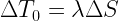
Appendix A : The One-Line Equation
The equation that Paul_K, Isaac Held, and I have used to replicate the climate models is as follows:
![]()
Let me break this into four chunks, separated by the equals sign and the plus signs, and translate each chunk from math into English. Equation 1 means:
This year’s temperature (T1) is equal to
Last years temperature (T0) plus
Climate sensitivity (λ) times this year’s forcing change (∆F1) times (one minus the lag factor) (1-a) plus
Last year’s temperature change (∆T0) times the same lag factor (a)
Or to put it another way, it looks like this:
T1 = <— This year’s temperature [ T1 ] equals
T0 + <— Last year’s temperature [ T0 ] plus
λ ∆F1 (1-a) + <— How much radiative forcing is applied this year [ ∆F1 (1-a) ], times climate sensitivity lambda ( λ ), plus
∆T0 a <— The remainder of the forcing, lagged out over time as specified by the lag factor “a”
The lag factor “a” is a function of the time constant “tau” ( τ ), and is given by
![]()
This factor “a” is just a constant number for a given calculation. For example, when the time constant “tau” is four years, the constant “a” is 0.78. Since 1 – a = 0.22, when tau is four years, about 22% of the incoming forcing is added immediately to last years temperature, and rest of the input pulse is expressed over time.
Appendix B: Physical Meaning
So what does all of that mean in the real world? The equation merely reflects that when you apply heat to something big, it takes a while for it to come up to temperature. For example, suppose we have a big brick in a domestic oven at say 200°C. Suppose further that we turn the oven heat up suddenly to 400° C for an hour, and then turn the oven back down to 200°C. What happens to the temperature of the big block of steel?
If we plot temperature against time, we see that initially the block of steel starts to heat fairly rapidly. However as time goes on it heats less and less per unit of time until eventually it reaches 400°C. Figure B2 shows this change of temperature with time, as simulated in my spreadsheet for a climate forcing of plus/minus one watt/square metre. Now, how big is the lag? Well, in part that depends on how big the brick is. The larger the brick, the longer the time lag will be. In the real planet, of course, the ocean plays the part of the brick, soaking up
The basic idea of the one-line equation is the same tired claim of the modelers. This is the claim that the changing temperature of the surface of the planet is linearly dependent on the size of the change in the forcing. I happen to think that this is only generally the rule, and that the temperature is actually set by the exceptions to the rule. The exceptions to this rule are the emergent phenomena of the climate—thunderstorms, El Niño/La Niña effects and the like. But I digress, let’s follow their claim for the sake of argument and see what their models have to say. It turns out that the results of the climate models can be described to 99% accuracy by the setting of two parameters—”tau”, or the time constant, and “lambda”, or the climate sensitivity. Lambda can represent either transient sensitivity, called TCR for “transient climate response”, or equilibrium sensitivity, called ECS for “equilibrium climate sensitivity”.
 Figure B2. One-line equation applied to a square-wave pulse of forcing. In this example, the sensitivity “lambda” is set to unity (output amplitude equals the input amplitude), and the time constant “tau” is set at five years.
Note that the lagging does not change the amount of energy in the forcing pulse. It merely lags it, so that it doesn’t appear until a later date.
So that is all the one-line equation is doing. It simply applies the given forcing, using the climate sensitivity to determine the amount of the temperature change, and using the time constant “tau” to determine the lag of the temperature change. That’s it. That’s all.
The difference between ECS (climate sensitivity) and TCR (transient response) is whether slow heating and cooling of the ocean is taken into account in the calculations. If the slow heating and cooling of the ocean is taken into account, then lambda is equilibrium climate sensitivity. If the ocean doesn’t enter into the calculations, if the forcing is only the radiative forcing, then lambda is transient climate response.
Appendix C. The Spreadsheet
In order to be able to easily compare the various forcings and responses, I made myself up an Excel spreadsheet. It has a couple drop-down lists that let me select from various forcing datasets and various response datasets. Then I use the built-in Excel function “Solver” to iteratively calculate the best combination of the two parameters, sensitivity and time constant, so that the result matches the response. This makes it quite simple to experiment with various combinations of forcing and responses. You can see the difference, for example, between the GISS E model with and without volcanoes. It also has a button which automatically stores the current set of results in a dataset which is slowly expanding as I do more experiments.
In a previous post called Retroactive Volcanoes, (link) I had discussed the fact that Otto et al. had smoothed the Forster forcings dataset using a centered three point average. In addition they had added a trend fromthe beginning tothe end of the dataset of 0.3 W per square meter. In that post I had I had said that the effect of that was unknown, although it might be large. My new spreadsheet allows me to actually determine what the effect of that actually is.
It turns out that the effect of those two small changes is to take the indicated climate sensitivity from 2.8 degrees/doubling to 2.3° per doubling.
One of the strangest findings to come out of this spreadsheet was that when the climate models are compared each to their own results, the climate sensitivity is a simple linear function of the ratio of the trends of the forcing and the response. This was true of both the individual models, and the average of the 19 models studied by Forster. The relationship is extremely simple. The climate sensitivity lambda is 1.07 times the ratio of the trends for the models alone, and equal to the trends when compared to all the results. This is true for all of the models without adding in the ocean heat content data, and also all of the models including the ocean heat content data.
In any case I’m going to have to convert all this to the computer language R. Thanks to Stephen McIntyre, I learned the computer language R and have never regretted it. However, I still do much of my initial exploratory forays in Excel. I can make Excel do just about anything, so for quick and dirty analyses like the results above I use Excel.
So as an invitation to people to continue and expand this analysis, my spreadsheet is available here. Note that it contains a macro to record the data from a given analysis. At present it contains the following data sets:
IMPULSES
Pinatubo in 1900
Step Change
Pulse
FORCINGS
Forster No Volcano
Forster N/V-Ocean
Otto Forcing
Otto-Ocean ∆
Levitus watts Ocean Heat Content ∆
GISS Forcing
GISS-Ocean ∆
Forster Forcing
Forster-Ocean ∆
DVIS
CM2.1 Forcing
CM2.1-Ocean ∆
GISS No Volcano
GISS GHGs
GISS Ozone
GISS Strat_H20
GISS Solar
GISS Landuse
GISS Snow Albedo
GISS Volcano
GISS Black Carb
GISS Refl Aer
GISS Aer Indir Eff
RESPONSES
CCSM3 Model Temp
CM2.1 Model Temp
GISSE ModelE Temp
BEST Temp
Forster Model Temps
Forster Model Temps No Volc
Flat
GISS Temp
HadCRUT4
You can insert your own data as well or makeup combinations of any of the forcings. I’ve included a variety of forcings and responses. This one-line equation model has forcing datasets, subsets of those such as volcanoes only or aerosols only, and the simple impulses such as a square step.
Now, while this spreadsheet is by no means user-friendly, I’ve tried to make it at least not user-aggressive.
Appendix D: The Mathematical Derivation of the Relationship between Climate Sensitivity and the Trend Ratio.
I have stated that the relationship where climate sensitivity is equal to the ratio between trends of the forcing and response datasets.
We start with the one-line equation:
![]()
Let us consider the situation of a linear trend in the forcing, where the forcing is ramped up by a certain amount every year. Here are lagged results from that kind of forcing.

Figure B1. A steady increase in forcing over time (red line), along with the situation with the time constant (tau) equal to zero, and also a time constant of 20 years. The residual is offset -0.6 degrees for clarity.
Note that the only difference that tau (the lag time constant) makes is how long it takes to come to equilibrium. After that the results stabilize, with the same change each year in both the forcing and the temperature (∆F and ∆T). So let’s consider that equilibrium situation.
Subtracting T0 from both sides gives
![]()
Now, T1 minus T0 is simply ∆T1. But since at equilibrium all the annual temperature changes are the same, ∆T1 = ∆T0 = ∆T, and the same is true for the forcing. So equation 2 simplifies to
![]()
Dividing by ∆F gives us

Collecting terms, we get

And dividing through by (1-a) yields

Now, out in the equilibrium area on the right side of Figure B1, ∆T/∆F is the actual trend ratio. So we have shown that at equilibrium

But if we include the entire dataset, you’ll see from Figure B1 that the measured trend will be slightly less than the trend at equilibrium.
And as a result, we would expect to find that lambda is slightly larger than the actual trend ratio. And indeed, this is what we found for the models when compared to their own results, lambda = 1.07 times the trend ratio.
When the forcings are run against real datasets, however, it appears that the greater variability of the actual temperature datasets averages out the small effect of tau on the results, and on average we end up with the situation shown in Figure 4 above, where lambda is experimentally determined to be equal to the trend ratio.
Appendix E: The Underlying Math
The best explanation of the derivation of the math used in the spreadsheet is an appendix to Paul_K’s post here. Paul has contributed hugely to my analysis by correcting my mistakes as I revealed them, and has my great thanks.
Climate Modeling – Abstracting the Input Signal by Paul_K
I will start with the (linear) feedback equation applied to a single capacity system—essentially the mixed layer plus fast-connected capacity:
C dT/dt = F(t) – λ *T Equ. A1
Where:-
C is the heat capacity of the mixed layer plus fast-connected capacity (Watt-years.m-2.degK-1)
T is the change in temperature from time zero (degrees K)
T(k) is the change in temperature from time zero to the end of the kth year
t is time (years)
F(t) is the cumulative radiative and non-radiative flux “forcing” applied to the single capacity system (Watts.m-2)
λ is the first order feedback parameter (Watts.m-2.deg K-1)
We can solve Equ A1 using superposition. I am going to use timesteps of one year.
Let the forcing increment applicable to the jth year be defined as fj. We can therefore write
F(t=k ) = Fk = Σ fj for j = 1 to k Equ. A2
The temperature contribution from the forcing increment fj at the end of the kth
year is given by
ΔTj(t=k) = fj(1 – exp(-(k+1-j)/τ))/λ Equ.A3
where τ is set equal to C/λ .
By superposition, the total temperature change at time t=k is given by the summation of all such forcing increments. Thus
T(t=k) = Σ fj * (1 – exp(-(k+1-j)/τ))/ λ for j = 1 to k Equ.A4
Similarly, the total temperature change at time t= k-1 is given by
T(t=k-1) = Σ fj (1 – exp(-(k-j)/τ))/ λ for j = 1 to k-1 Equ.A5
Subtracting Equ. A4 from Equ. A5 we obtain:
T(k) – T(k-1) = fk*[1-exp(-1/τ)]/λ + ( [1 – exp(-1/τ)]/λ ) (Σfj*exp(-(k-j)/τ) for j = 1 to k-1) …Equ.A6
We note from Equ.A5 that
(Σfj*exp(-(k-j)/τ)/λ for j = 1 to k-1) = ( Σ(fj/λ ) for j = 1 to k-1) – T(k-1)
Making this substitution, Equ.A6 then becomes:
T(k) – T(k-1) = fk*[1-exp(-1/τ)]/λ + [1 – exp(-1/τ)]*[( Σ(fj/λ ) for j = 1 to k-1) – T(k-1)] …Equ.A7
If we now set α = 1-exp(-1/τ) and make use of Equ.A2, we can rewrite Equ A7 in the following simple form:
T(k) – T(k-1) = Fkα /λ – α * T(k-1) Equ.A8
Equ.A8 can be used for prediction of temperature from a known cumulative forcing series, or can be readily used to determine the cumulative forcing series from a known temperature dataset. From the cumulative forcing series, it is a trivial step to abstract the annual incremental forcing data by difference.
For the values of α and λ, I am going to use values which are conditioned to the same response sensitivity of temperature to flux changes as the GISS-ER Global Circulation Model (GCM).
These values are:-
α = 0.279563
λ = 2.94775
Shown below is a plot confirming that Equ. A8 with these values of alpha and lamda can reproduce the GISS-ER model results with good accuracy. The correlation is >0.99.

This same governing equation has been applied to at least two other GCMs ( CCSM3 and GFDL ) and, with similar parameter values, works equally well to emulate those model results. While changing the parameter values modifies slightly the values of the fluxes calculated from temperature , it does not significantly change the structural form of the input signal, and nor can it change the primary conclusion of this article, which is that the AGW signal cannot be reliably extracted from the temperature series.
Equally, substituting a more generalised non-linear form for Equ A1 does not change the results at all, provided that the parameters chosen for the non-linear form are selected to show the same sensitivity over the actual observed temperature range. (See here for proof.)
Bloody brilliant. I love maths. You cannot be wrong if the answer is correct it takes you back to the question.
Willis, you are a bloody genius.
There’s only one factor that you left out, which I think is very important: the amount of warming predicted is directly proportional to the amount of funding expected to be realized by said prediction. Which leads to the corollary: A climate modeler’s Income stream is inversely proportional to the amount of cooling which he allows his model to show.
Brilliant. Simply brilliant.
(Look forward to seeing the R results as it would be a worthwhile project for me to learn both R and this modelling issue.)
Without assumed water vapor feedback, CS is one degree C or less for first CO2 doubling. Unfortunately for the Team, this key but evidence-free assumption has been shown false by the only “climate science expert” who counts, Mother Nature.
err
I pointed this out to you back in 2008
http://climateaudit.org/2008/05/09/giss-model-e-data/#comment-148141
http://rankexploits.com/musings/2008/lumpy-vs-model-e/
nothing surprising about this. You can fit the super complicated Line by Line radiative transfer models with a simple function delta forcing = 5.35ln(C02a/C02b)
Finally
‘Now, I don’t have the ocean forcing data that was used by the models. ”
there is no ocean forcing data. Forcings are all radiative components. The ocean is forced.
the atmosphere is forced. the land is forced. They respond to this forcing.
I’m not a climatologist, but I’ve built a number of models to forecast and/or assign to specific traffics the costs of a shared transportation network. I’ve found, generally, that no matter how many complex factors are included, there are usually only one or two that determine the result. It’s nice to know that is true for climate models as well.
• λ ∆F1 (1-a) + <— How much radiative forcing is applied this year [ ∆F1 (1-a) ], times climate sensitivity lambda
—–
So, all the warmists need do is be able to predict annual radiative forcings for the next century and their predictions will spot on allowing for spikes like eruptions. Wait. How are they doing with SC 24? Not so good eh.
I say the warmists should release all their funding towards solar modeling.
It should be obvious that CO2 is among the least important potential climate forcings. Mean global T, as nearly as can be reconstructed, was about the same at 7000 ppm & 700. It was also about the same as today with carbon dioxide at 4000 to 7000 ppm during the Ordovician glaciation, although the sun was four percent cooler then.
Billions of dollars & hordes of researchers for something I could do w/a slide rule….
What is it with climate scientists? Not only did they all appear to have skipped statistics classes, they appear to have skipped the philosophy of science courses as well.
“entities must not be multiplied beyond necessity” was written by John Punch from Cork in 1639, although generally referred to as Occam’s Razor.
Excellent work, Willis.
[…] So … my new finding is that the climate sensitivity of the models, both individual models and on average, is equal to the ratio of the trends of the forcing and the resulting temperatures. This is true whether or not the changes in ocean heat content are included in the calculation. It is true for both forcings vs model temperature results, as well as forcings run against actual temperature datasets. It is also true for subsets of the forcing, such as volcanoes alone, or for just GHG gases.[…]”
==================================================================
How do you make a jaw-dropper emoticon? wOw!
P.S. I want my tax money back. Meanwhile, they can pay Willis his usual day rate for the same results – what the heck! 2-3x(day rate) – and put how many billions back in our pockets?
But since at equilibrium all the annual temperature changes are the same, ∆T1 = ∆T0 = ∆T, and the same is true for the forcing.
At equilibrium, all of the temperature changes and forcing changes are 0. The first is the definition of equilibrium,, and the second is one of the necessary conditions for an equilibrium to be possible.
As you wrote, you have modeled the models, but you have not modeled the climate. You have taken two time series, modeled temperature and forcing, where modeled temperature is a function of the forcing. From those two correlated time series you have written modeled T as a linear function of changed forcing and changed temperature, where the two changes are not computed on the same interval.
“Energy Secretary Ed Davey is to make an unprecedented attack later on climate change sceptics.”
http://www.bbc.co.uk/news/science-environment-22745578
“n a speech, the Lib Dem minister will complain that right-wing newspapers are undermining science for political ends.”
Pot to kettle!!!
Thanks Willis! Saves a lot of time and effort and headaches to have a simple expression like this to approximate climate models, looking forward to playing around with this.
Steven Mosher says:
June 3, 2013 at 12:04 pm
“nothing surprising about this. You can fit the super complicated Line by Line radiative transfer models with a simple function delta forcing = 5.35ln(C02a/C02b)”
Yet you still think it is not a pseudoscience?
Matthew writes: “… you have modeled the models, but you have not modeled the climate.”
That’s exactly the point. The models do not model the climate either, and are in effect just a representation of the forcing assumptions input to them.
This makes intuitive sense and long over-due to be articulated in such a clear way – thanks. Climate modellers have always been quick to demonstrate how well they can hindcast, but really they’re just saying 2 + 2 – 4 = 0 and congratulating each other on figuring out the third parameter was 4. Of course their colleague was solving 2 + 6 – 8 = 0 which is equally impressive and worthy of funding. I don’t have the reference in front of me, but I recall at least one GCM being criticized for including an interactive “solver” type application integrated into the parameter setting process to handle just such gaming.
I’m happy that Willis is understanding some of the math in simple one-line climate models, but as Steve Mosher has alluded to, there is really nothing new here. Of course the global average behavior of a complex 3-D climate model can be accurately approximated with a 0-D model, mainly because global average temperature change is just a function of energy in (forcings) versus energy out (feedbacks). But that really doesn’t help us know whether either one has anything to do with reality.)
Willis, you are a smart guy and a quick learner, and you have a talent for writing. Try to understand what has already been done, and build upon that… rather than reinventing it.
It shows again, what i suspected, that the climate models only makes it all look more scientific by wrapping it in super complicated programming.
The models have value when you analyse parts of the climate or weather, but when you take the average of the whole earth, and on top of that average over a year or more and then furthermore average over 30+ models, then the only part left is the forcings and sensitivity.
I have seen it stated from different sources, that it more or less is so.
Wow, respect to you for this. Are you expecting the “Big Oil” check to arrive soon?
🙂
Blinded me with science.
You da man with the math.
to paraphrase you: So many variables, so little time. (or is that dimes)
Steven Mosher says:
June 3, 2013 at 12:04 pm
err … you pointed out exactly what to me in 2008? Once again, your cryptic posting style betrays you, and the citations are of little help. A précis would be useful …
If that is what you pointed out, actually it is quite surprising that the climate models can be represented by a simple equation. There are models, and there are models. The climate models are massively complex, and more importantly, iterative models designed to model a chaotic system. Those kinds of models should definitely not be able to have their outputs replicated by a simple one-line equation.
In addition, when you find the simple model that represents the complex LBL model, you don’t sneer at it as you have done with my simple model. You USE it, right? Once you find the simple model “delta forcing = 5.35ln(C02a/C02b)”, you often, even usually don’t need to use the complex line-by-line model in your further calculations. And that is exactly what I have done here, USED the simple model to find further insights into the relationships.
Finally, none of your objections touch the really interesting result, which is that the climate sensitivity given by the climate models is simply the trend ratio …
Sorry for the shorthand. The radiative forcing doesn’t all go to warm the surface. Some of it warms the ocean as well. I have referred to the part of the radiative forcing which has gone into the secular warming trend of the ocean as “ocean forcing”, expressed the annual change in W/m2, and subtracted it from the radiative forcing. This gives the net forcing which warms the surface … at least in their simplistic theory.
Best regards,
w.
Hi Willis
I use one equation & single forcing .
Fascinating and intuitively convincing (from what I know about modelling) BUT a passing comment and a friendly warning – and if you are already aware of this, my apologies, Spreadsheets generally and Excel in particular can be false friends. I was involved in a UK government programme on software quality which had as one theme, the dangers of dependence on the internal mathematics/functions in spreadsheets in critical calculations. We were mainly looking at metrological (rather than meteorological!) applications but the point was that the internal functions/algorithms in spreadsheets, particularly Exel, could not be safely depended upon if the data concerned was other than very straightforward. We found some of the more specifically science oriented packages were much more reliable. This was a few years ago but I think you may still find some more reliable and tested algorithms that can be plugged into Exel on the NPL website at http://www.npl.gov.uk/ssfm/ – ssfm was the software support for metrology programme (excuse the British spelling).
Roy Spencer says:
June 3, 2013 at 12:33 pm
Roy, with all due respect, you are a smart guy as well, but first, show me anywhere that anyone has derived the relationship that the climate sensitivity of the models is merely the trend ratio of the input and output datasets.
If you cannot do that, and I’ve never seen it, then your objection misses the point.
Second, as a long-time computer modeler of all types of systems, I assure you that there is absolutely no “of course” that the output of a complex 3-D iterative model of a chaotic system can be replicated by a simple one-line equation. Please give me some examples if you think this is a common thing. You might start by contemplating the input and output states of Conway’s game of “Life”, an extremely simple 2D iterative model, and see if you can represent the state of the output with a 0-D model … good luck.
Finally, you say that this “really doesn’t help us know whether either one has anything to do with reality”. In fact it does, because the simple model shows us that the climate model results have nothing to do with reality. Paul_K has shown that result mathematically for the entire simple 0-D model, and I have shown it with respect to the sensitivities shown by that model.
w.
Yes I agree climate models based on the political decided UNFCCC are unscientific and are with 99 % certainty WRONG
Hi Willis,
This is fairly common in engineering (that a complex system can be modeled by a simple equation over limited conditions/time-frame). As useful as that can be, it does not demonstrate understanding of the complex system- it merely means you can predict behavior over some limited range. OK, so what? Well, often that’s good enough. I’ll say that again, often that’s good enough.
The problem is when a real event occurs that invalidates the simple equation (black box) and the black box no longer produces useful output. So there’s a difference between something that’s useful, and really understanding what’s under the hood.
In the long run, you are better off understanding the complex system, but folks should understand that’s not required for something to be useful.
it is their way to keep energy conservation under control?
Matthew R Marler says:
June 3, 2013 at 12:23 pm
Apologies for the lack of clarity, Matt, I should have said “steady state” rather than “equilibrium”, as the forcing and temperature are both continually rising (see figure B1).
w.
Willis, I think you have found an underlying fact about the current status of climate science. Since 1980’s there has really been only cosmetic changes in AGR predictions despite an order of magnitude increase in resolution and complexity of GCM models. Most of the “progress” (IMHO) seems to have been in fine tuning various “natural/anthropogenic” variations in aerosols to better fit past temperature response. Uncertainties still remain about natural feedbacks – especially clouds. Looking at your equation.
 where
where  is the transient temperature response and
  is the equilibrium temperature response.


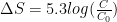 , where C and C0 are the values before and after the yearly pulse. All values are calculated from seasonally averaged Mauna Loa data smoothed back to an initial concentration of 280ppm in 1750.
 was calculated based on an assumed ECS of 2.0C. The results can then be compared to the observed HADCRUT4 temperature anomalies – see here.
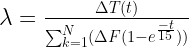
Tau is the relaxation time for the climate system to react to any sudden change in forcing. This could be a volcano, a meteor, aerosols or CO2. Climate models including ocean/atmosphere interactions (for example GISS) seem to point to a value for Tau of ~ 10-15 years. Your equation works by simply taking direct CO2 forcing (MODTRAN) each year to be DF = 5.3ln(C/C0), where C-C0 = the increase measured using the Mauna Loa data extrapolated back to 1750. So simply taking lambda as the climate sensitivity (hoping latex works!)
and then taking Stefan Boltzman to derive the IR energy balance
or in terms of feedbacks
and for equilibrium climate sensitivity for a doubling of CO2
To calculate the CO2 forcing take a yearly increment of
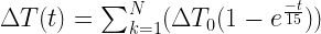
Each pulse is tracked through time and integrated into the overall transient temperature change using:
If we assume an underlying 60 year natural oscillation (AMO?) superimposed onto a CO2 AGW signal then at worst ECS works out to be ~2C.
more details – here
One line equations may work to emulate the crude GISS models but there is talk around town that the NCAR/UCAR CESM takes computational and algorithmic advantage of the vibrations of the massive crystal dome under the City of Boulder. There is no way to simplify and match that.
which is that the climate sensitivity given by the climate models is simply the trend ratio …
======
woops…..so even if they are putting in all of the other crap……all that stuuf is doing is cancelling itself out
If 2 computer systems are functionally equivalent, that is they produce the same outputs from the same inputs, then they are logically equivalent, that is the operations of one can be transformed into the operations of the other.
Which means 99.99% of the code in the climate models doesn’t actually do anything significant to the outputs. And buried within them is the logical equivalent of Willis’ equation.
The climate modellers must surely know this.
Roy Spencer says:
June 3, 2013 at 12:33 pm
Coming from a simulation background I’ve been saying for years that all they did was pick a CS they liked, and then adjusted the other knobs until they liked the results.
But what’s really telling is that their 3D results aren’t very good, it’s only when they average them all together that they have something they can print while not hiding their faces.
and
Basically they can’t simulate any random specific area correctly, but it’s close if they average all of their errors together.
So essentially, we have paid a trillion dollars for this equation and published (apparently) 100,000+ papers on it, and Willis has reduced all the bumph down to an equation with an R^2 fit of 1.00. Mosher says this is nothing new here, but in the previous post when Willis used this equation as the blackbox equation, he protested that this isn’t the equation used by IPCC nobility – a disengenuous critique, with what he apparently knew already. Roy Spencer made the same criticism but I would argue to these two gentlemen that all the rest of us got a hell of a good education out of his effort because those in the know weren’t prepared to present this revelation to the great unwashed. The consensus synod has less to sneer and much to fear from the work of this remarkable man.
MJB says:
June 3, 2013 at 12:31 pm
“of funding. I don’t have the reference in front of me, but I recall at least one GCM being criticized for including an interactive “solver” type application integrated into the parameter setting process to handle just such gaming.”
WHAT? It is frowned upon when they train the parameterization automatically? It is expected that they do it manually? What for? To uphold a pretense of scientific activity? The cult is getting ridiculouser by the day.
In electronics, Thevenin’s* theorem states that any linear black box circuit, no matter how complicated, can be replaced with a voltage source and an impedance. Since a linear circuit, no matter how complicated, is modeled by a set of linear equations, we can extrapolate that any set of linear equations can be replaced by one linear equation if all we want is the overall system response.
Your results make it a pretty good bet that the climate models are predominantly linear. Given that we’re talking about thermodynamics, … yep, I think that might be a problem.
=============================================
*http://en.wikipedia.org/wiki/Th%C3%A9venin%27s_theorem Thevenin is a great shortcut for circuit analysis, nothing more.
Steven Mosher says:
June 3, 2013 at 12:04 pm
“err
I pointed this out to you back in 2008
http://climateaudit.org/2008/05/09/giss-model-e-data/#comment-148141
http://rankexploits.com/musings/2008/lumpy-vs-model-e/
nothing surprising about this. You can fit the super complicated Line by Line radiative transfer models with a simple function delta forcing = 5.35ln(C02a/C02b)”
_____________________
You really should ripen those sour grapes before you try to sell ’em… they are (again) making it appear that you are attempting obfuscation.
~~~~~~~~~~~~~~~~~~~~~
MiCro says:
June 3, 2013 at 1:35 pm
“Coming from a simulation background I’ve been saying for years that all they did was pick a CS they liked, and then adjusted the other knobs until they liked the results.”
_________________________
Yes indeed. That’s the way it’s looked for quite some time. (won’t mention harryreadme)
~~~~~~~~~~~~~~~~~~~~~~~~~
Willis Eschenbach says:
June 3, 2013 at 1:14 pm
Matthew R Marler says:
June 3, 2013 at 12:23 pm
“But since at equilibrium all the annual temperature changes are the same, ∆T1 = ∆T0 = ∆T, and the same is true for the forcing.
At equilibrium, all of the temperature changes and forcing changes are 0. The first is the definition of equilibrium,, and the second is one of the necessary conditions for an equilibrium to be possible.”
“Apologies for the lack of clarity, Matt, I should have said “steady state” rather than “equilibrium”, as the forcing and temperature are both continually rising (see figure B1).”
w.
__________________
Fine work, nevertheless. Many thanks.
~~~~~~~~~~~~~~~~~~~~
The fact that a GCM can match temperature and heat data tells us nothing about the validity of that GCM’s estimate of Equilibrium Climate Sensitivity.
+++++++++++++++++
Only the climate models with the correct Equilibrium Climate Sensitivity would be able hind-cast past temperatures. However, multiple models with different ECS can all hind-cast past temperatures. Which either means that ECS doesn’t determine temperature, or the models are faulty.
Matthew R Marler says:
June 3, 2013 at 12:23 pm
As you wrote, you have modeled the models, but you have not modeled the climate.
========
since it is quite clear that the models haven’t modeled climate, anything that models the models is also not going to model climate.
The models are pretty simple really. Each cell in the atm has a set of inputs and outputs on each side, plus top and bottom. There’s a set of rules that does the math based on each in, and propagates the results to each output. There are cells who’s sides are dirt, and by now ones who’s sides are water. There are 14-15 cells for each area from the a little below the surface up to space. And a grid of cells to cover the earth, the more cells the more accurate the results are, but the longer the simulations take to run. Climatologists have been insisting that the reason they’re results are off is they can’t make the grids small enough. So bigger computers are required.
When it’s initialize, without stepping “time”, inputs are propagated to output until the outputs become stable. This accounts for the output of one cell changing the input of another. They do this until each cell initialized to the state it’s defined to be, then they provide a forcing, and let the clock step forward one clock tick, then each cell runs it’s calculations until the output stabilizes. Then they step the clock, and repeat.
This is the same process used by linear simulators like SPICE, in fact you could replicate the equations of each cell with spice, it would just be really slow, and more difficult to twist knobs on.
But it’s just a bunch of equations to solve.
This link is to a very good document on the basics of GCM’s.
commieBob says:
June 3, 2013 at 1:53 pm
“Thevenin’s theorum…”
_____________________
Yep. I’ve never been able to look at the any statement about climate models without visions of Thevenin- Norton equivalents and Kirchoff equations zapping through what’s left of my brain.
Philip Bradley says:
June 3, 2013 at 1:33 pm
I
I doubt it. The climate models, like Topsy, have “jes’ growed”. In addition, it’s a recurring problem with iterative models, which is that even if you get the “right” answer, you don’t know how you got there … but my “black box” analysis shows how. So I don’t think the modelers knew that.
w.
Nice work, Willis and collaborators. As with all clear math, beautiful and compelling.
Another answer to Dr. Spencer is that his comment applies to figure three, but not to an important part of figure four and smacks of sour grapes, especially since his own recent simple model did not work out so well.
A comment is surprising that so many different GCM models (and an ensemble!) gave ‘exactly’ the same trend ratio answer to the relationship between forcing input and temperature output, even though from figures two and three obviously not the same lambda, showing the models themselves do differ in important sensitivity respects (itself primarily driven by positive water vapor feedback and clouds, since the ‘feedback neutral’ sensitivity from Stefan-Boltsmann is always between 1( theoretical black body) and model grid specific, real earth ‘grey body’ 1.2).
A possible reason is that each model is ‘tuned’ (parameterized with things like aerosols and within grid cell cloud and convection microprocesses) to hind cast past temperature as accurately as possible. Even though those tunings differ by model, they all produce the same temperature result, so by intent the same trend ratio as evidenced in Figures 2 and 3. Another way to show that they are therefore unlikely to accurately predict the future temperature or true sensitivity, as you have already observed.
It will be most interesting to learn what you and your collaborators do next with these most interesting results. One suggestion might be to use the one line equation and it’s corollaries to ‘filter out’ the known forcings (like CO2) temperature consequences to estimate the ‘natural’ variability of temperature over the periods where data of different levels of certainty exists. Satellite era greatest, 1880 or so least. Said differently your new tools might go a long way on the attribution problem. Can a 60 year natural cycle be extracted? Can the pause be explained as a function of whatever happened from 1945-1965? Lots of potentially interesting stuff, without spending more billions to spin up the supercomputers for months at a pass.
Willis,
“So … my new finding is that the climate sensitivity of the models, both individual models and on average, is equal to the ratio of the trends of the forcing and the resulting temperatures.”
I think calculus gives a reason for this. Idealized,
trend_T≅dT/dt, trend_F≅dF/dt
and, with many caveats as discussed in your previous thread,
λ≅dT/dF=(dT/dt)/(dF/dt)=trend_T/trend_F
Willis – I am surprised that you are surprised by what you found. It is an inevitable result of their process.. See IPCC report AR4 Ch.9 Executive Summary : “Estimates of the climate sensitivity are now better constrained by observations.“. “constrained by observation” means that they constrained their models in order to get climate sensitivity to match observed temperature. Forcings are the primary inputs to the models, so across the models you must necessarily get the relationship that you noticed.
Rud Istvan says:
June 3, 2013 at 2:09 pm
Thanks for your kind words, Rud. I wish I had collaborators, it’s just me and my computer.
Regarding what’s next, I want to apply the equations on a gridcell-by-gridcell basis using the CERES data. As you point out, the interesting thing about the one-line equation is that we can use it to see both when and where the climate is NOT responding as expected to the forcing.
w.
Rud Istvan says:
June 3, 2013 at 2:09 pm
This is because they’re all almost identical, at most they adjust the equations in the cells, mostly they just set the knobs differently.
Mod, I think my last post got eaten, can you check for it? this post will make more sense after reading the last one.
[Reply: Prior comment found in Spam folder. Rescued & posted. — mod.]
Colorado Wellington says:
June 3, 2013 at 1:21 pm
One line equations may work to emulate the crude GISS models but there is talk around town that the NCAR/UCAR CESM takes computational and algorithmic advantage of the vibrations of the massive crystal dome under the City of Boulder. There is no way to simplify and match that.
_____________________
I’m keepin’ an eye on you, dude. It’s not clear yet whether you are a man of good humor or if you simply moved to Boulder to get higher. Or something.
PS. Willis – I don’t want that last comment of mine to be taken as critical of your analysis. What you have done, very succinctly, is to show that they really did do what they said they did, but you have done it in a way that shows people very clearly how that renders the models useless for most purposes, and why the IPCC say they only do “projections” not predictions. The crying shame is that people have deliberately been led to believe that the models make predictions which can sensibly be used for policy purposes.
What Willis is presenting is a difference equation that replicates the global average of the climate models. The very same average that climate modellers themselves put forward as a prediction of future temperatures.
Far from being trivial, difference equations are used routinely as a shorthand method to model dynamic systems such as weather and climate that are derived from differential equations. When two methods calculate the same answer, and one takes seconds and costs pennies, and the other takes years and costs hundreds of millions, the one that takes seconds is significantly more valuable than the method that takes years. Every time it runs it saves millions of dollars. Computer Science invests millions each year in trying to find faster numerical methods to solve problems.
For example:
Difference Equations and Chaos in Mathematica
Dr. Dobb’s Journal
Year: 1997
Issue: November
Page range: 84-90
Description
A difference equation (or map) of the form x_n-1 = f(x_n, x_n-1, …) which, together with some specified values or initial conditions defines a sequence {x_n}. Despite the seemingly simple form, difference equations have a variety of applications and can display a range of dynamics. Since maps describe iterative processes, they come up frequently in computer science. Also, many of the approximations in numerical analysis (such as numerical solutions of differential equations) typically approximate continuous dynamical systems using discrete systems of difference equations. Modeling a map using a computer is equivalent to studying the process of functional composition or functional iteration.
http://library.wolfram.com/infocenter/Articles/1032/
Steve McIntyre is plainly a friend of Willis. Also, Phil Jones obviously has none, at least within climate science.
DirkH says:
June 3, 2013 at 12:26 pm
Steven Mosher says:
June 3, 2013 at 12:04 pm
“nothing surprising about this. You can fit the super complicated Line by Line radiative transfer models with a simple function delta forcing = 5.35ln(C02a/C02b)”
Yet you still think it is not a pseudoscience?
###########
Understand what Willis has done. He’s done what we do all the time in modelling.
you take a complex system that outputs thousands of variables. You pick a high level
general metric ( like global temperature )
You fit the inputs to that output.
You now have a model of the model or an emulation of the model.
What this emulation cant do is tell you about regional climate, or SST by itself
or arctic amplification.
getting this kind of fit is a good test of the model.. which is why as an old modler I suggested it years ago. This is nothing new.
There are other ways to do this that are more sophisticated ( and give you spatial fields) iits one of the ways you can find bugs in the models. I’ve posted on that as well.
ferd berple says:
June 3, 2013 at 2:05 pm
Re: Matthew R Marler
Heh.
Luther Wu says:
June 3, 2013 at 2:17 pm
Still trying to sort it out myself. ”Or something” is the safest bet.
Mike Jonas writes : “What you have done, very succinctly, is to show that they really did do what they said they did, but you have done it in a way that shows people very clearly how that renders the models useless for most purposes, and why the IPCC say they only do “projections” not predictions. The crying shame is that people have deliberately been led to believe that the models make predictions which can sensibly be used for policy purposes.”
This is spot on. The models accurately reproduce past temperature change because they fine tune natural/aerosol “forcings”. They have little predictive value because they cannot know in advance how such future natural forcing will evolve. That is why their “projections” fan out with massive error bars to 2100 in order to cover all eventualities.
Philip Bradley says:June 3, 2013 at 1:33 pm
“If 2 computer systems are functionally equivalent, that is they produce the same outputs from the same inputs, then they are logically equivalent, that is the operations of one can be transformed into the operations of the other.
Which means 99.99% of the code in the climate models doesn’t actually do anything significant to the outputs. And buried within them is the logical equivalent of Willis’ equation.
The climate modellers must surely know this.”
This long GISSE paper will show you that models output a great deal more than just a time series of global average temperature. That’s what the code is doing.
Buried within them is energy conservation, which is the basis of the simple relations, as Roy Spencer says. Modellers do surely know that – they put a lot of effort into ensuring that mass and energy are conserved. But there are innumerable force balance relations too.
err … you pointed out exactly what to me in 2008? Once again, your cryptic posting style betrays you, and the citations are of little help. A précis would be useful …
##############
1. read the thread.
2. I suggested that Lucia use Lumpy to hindcast
3. I pointed out to you how well one could hindcast models with two parameter lumpy
more background here as the links have disappeared from the CA thread
http://rankexploits.com/musings/2008/lumpy-vs-model-e/
“nothing surprising about this. You can fit the super complicated Line by Line radiative transfer models with a simple function delta forcing = 5.35ln(C02a/C02b)
If that is what you pointed out, actually it is quite surprising that the climate models can be represented by a simple equation. There are models, and there are models. The climate models are massively complex, and more importantly, iterative models designed to model a chaotic system. Those kinds of models should definitely not be able to have their outputs replicated by a simple one-line equation.”
############
its Not at all surprising which is why i suggested to Lucia that she do this excercise back in 2008. it’s pretty well known. Its a standard technique called emulation. you emulate the model. This is STEP ONE in any sort of sensitivity analysis where the parameter space is too large to excercise in a full factorial manner.
################
In addition, when you find the simple model that represents the complex LBL model, you don’t sneer at it as you have done with my simple model. You USE it, right? Once you find the simple model “delta forcing = 5.35ln(C02a/C02b)”, you often, even usually don’t need to use the complex line-by-line model in your further calculations. And that is exactly what I have done here, USED the simple model to find further insights into the relationships.
#######
WHO SNEERED? why would i sneer at a experiment I proposed back in 2008?
Its cool. Its actually a good check on the models. but its not surprising. It tells you the models are working.
#############
Finally, none of your objections touch the really interesting result, which is that the climate sensitivity given by the climate models is simply the trend ratio …
Huh? refer to Nick’s calculus.
###############################
‘Now, I don’t have the ocean forcing data that was used by the models. ”
there is no ocean forcing data. Forcings are all radiative components. The ocean is forced.
the atmosphere is forced. the land is forced. They respond to this forcing.
Sorry for the shorthand.
No problem
” Understand what Willis has done. He’s done what we do all the time in modelling. you take a complex system that outputs thousands of variables. You pick a high level general metric ( like global temperature ) You fit the inputs to that output. You now have a model of the model or an emulation of the model. What this emulation cant do is tell you about regional climate, or SST by itself or arctic amplification.”
If it was really that simple, then instead of picking global temperature as your high-level metric, you could pick regional climate for one particular location, or Arctic amplification. Then fit the input to that output, and you have a simple one-line model that will tell you what the climate in Albuquerque will be in 2100, or whatever.
And then you would be able to tell people that you can project regional climates, too. Albeit, not all with the same model settings.
I’m not sure if this is a feature of a special property of the model equations, like global energy conservation, or if it’s just simple curve-fitting. If the latter, then it ought to work equally well for any 1D function of the output. And if so, then it would appear the big models can’t tell you anything about regional climate or SST or Arctic amplification either.
Willis Eschenbach: Apologies for the lack of clarity, Matt, I should have said “steady state” rather than “equilibrium”, as the forcing and temperature are both continually rising (see figure B1).
At “steady-state” the forcings and the temperatures are constant. At steady-state, the inflow and outflow of heat in any voxel, parcel, compartment (etc) of the climate system exactly balance, and the temperature remains constant. That’s the definition of “steady state.” A condition for the steady state to be possible is that overall input, what is called “forcing” in this context, be constant.
If you relax further and go to “stationary distribution” , then the changes have constant means, but they are not equal at all times. Figures 2 and 3 display interesting relationships between your parameter estimate lambda and the forcing, across models, but that’s all.
So , You are described your ability to recostruct with a simple two-parameter formula the total conservation of energy into the system.
Interesting but pretty useless. A model should do exactly this.
I would be surprised if models don’t conserve the Earth energy balance, which is a direct effect of radiative energy coming in (forcings) and going out, at the equilibrium temperature.
Or did you think that the Earth is a sponge adsorbing all energy and not releasing it? The problem of climate change is NOT the amount of energy, but the equilibrium temperature, and the distribution of it, and the effect on hidrosphere and biosphere.
I suppose that your “one line” model is not sufficiently evoluted to quantify sea level change and humidity distribution, don’t you?
Regards
Colorado Wellington says:
June 3, 2013 at 2:37 pm
Luther Wu says:
June 3, 2013 at 2:17 pm
I’m keepin’ an eye on you, dude. It’s not clear yet whether you are a man of good humor or if you simply moved to Boulder to get higher. Or something.
Still trying to sort it out myself. ”Or something” is the safest bet.
_______________________
A (much) earlier post of yours proved that you had a lick of sense.
One person told me yesterday that HAARP is behind the OKC tornadoes and they knew that because of the abrupt turns some number of storms have made to avoid prime targets such as Tinker Air Force Base (or my house.) Another person told me just this morning that God was cleaning up OKC because there are homosexuals here.
It’s a wild world, I tell ya.
Thanks Willis. As Gary says at 1:47pm : ” …all the rest of us got a hell of a good education out of [your] effort …”.
50 years ago I was in “remedial class” for maths and I can follow this.
[Maybe I’d better add that nothing I have designed or built since then has resulted in catastrophic failure.]
Next question is, which of these one liners to print on T-shirts?
Equation 1 might be ok for those of us who are horizontally challenged …
ferd berple: since it is quite clear that the models haven’t modeled climate, anything that models the models is also not going to model climate.
I have no quarrel with that. The obvious implication is that the parameter lambda is not related to anything in the climate, it’s just something that allows Willis’ model of forcing and model output to reproduce model output with high accuracy. I think it is remarkable that for all of their complexity, the models can be modeled by a really simple bivariate linear autoregressive model.
Matthew R Marler says:
June 3, 2013 at 3:04 pm
Thanks, Matt. You are talking about a different steady state. In Figure B1, both the forcing and the temperature are increasing at a steady rate. That’s the situation shown in that Figure, regardless of what you call it.
w.
Nullius in Verba says:
June 3, 2013 at 2:59 pm
And if so, then it would appear the big models can’t tell you anything about regional climate or SST or Arctic amplification either.
=============
Run a climate model twice, it should give you two different results, unless it is a trivial (unrealistic) model. Run it many times and the results give you a boundary. If the model is accurate, then future climate lies somewhere within that boundary, and the edges of the boundary give you natural variability.
However, no model can (accurately) tell you where within the boundary the future climate lies. The current climate science practice of averaging the runs and calling this the future is mathematical nonsense. Which is why the models have gone off the rails.
Roy Spencer says:
June 3, 2013 at 12:33 pm
Oh, Roy. I think you miss the point. So as a non-scientist, I will make it to you.
Science spends a lot of time trying to reduce difficult concepts and physical theories and observations down to one simple equation. I think that Stephen Hawking and field unification theories are the quintessential example of this striving. While this is the (admirable) goal of all science, after Einstein’s E=mc2 I think most scientists were so overawed by that equation that they started striving for that beauty and simplicity in all other areas of science (such as climate science), where such beauty and simplicity is simply not possible (at least, not possible without sacrificing much of the truth in the process). As a result, some scientists have reduced the world down to something that it really is not (Mosh appears to make that mistake constantly, as he shows in his dialogue with Willis here). The models may correlate well with one equation, but as the old saw about models and assumptions says: garbage in, garbage out. It is also called “missing the forest for the trees.”
Also, read “o sweet spontaneous” by e.e. cummings for a bit more of what I mean.
I suspect finding linear behavior is actually evidence that we are near an attractor. These kinds of simple formulas fall apart as the system gets away from the attractor and the system becomes more chaotic.
Richard M says:
June 3, 2013 at 3:23 pm
I suspect finding linear behavior is actually evidence that we are near an attractor. These kinds of simple formulas fall apart as the system gets away from the attractor and the system becomes more chaotic.
__________________
Since the system is already chaotic, “becoming more chaotic” could be viewed as increasing amplitudes of various forces/feedbacks, which system would still return to trend, wouldn’t it?
What sort of attractor do you envision?
This long GISSE paper will show you that models output a great deal more than just a time series of global average temperature. That’s what the code is doing.
Buried within them is energy conservation, which is the basis of the simple relations, as Roy Spencer says. Modellers do surely know that – they put a lot of effort into ensuring that mass and energy are conserved. But there are innumerable force balance relations too.
I should have been more precise and said,
Which means 99.99% of the code in the climate models doesn’t actually do anything significant to the surface temperature outputs.
The models may well be getting better at modelling at air column turbulence, etc, but these improvements have no significant effect on the surface temperature predictions. Therefore these model improvements are irrelevant to the metric everyone cares about. And 99.99% of the code in the models could removed without affecting the surface temperature predictions.
But hugely complicated ‘sophisticated’ climate models impresses the mug punter. Who would be decidedly unimpressed by a surface temperature prediction from a one line computer program. Even if you told him/her that the prediction from the one line program was identical to that from the ‘sophisticated’ model.
[snip – more Slayers junk science from the banned DOUG COTTON who thinks his opinion is SO IMPORTANT he has to keep making up fake names to get it across -Anthony]
Roy Spencer says:
June 3, 2013 at 12:33 pm
I’m happy that Willis is understanding some of the math in simple one-line climate models, but as Steve Mosher has alluded to, there is really nothing new here.
——————
Willis Eschenbach already answered on this.
Further, when the Met Office asks for the next new super computer, do British MPs and the public really know, that the main result could equally be computed on the back of an envelope ?
Steven Mosher says:
June 3, 2013 at 2:49 pm
Thanks, Steven. So your point is that you noted that the models could be fit with Lumpy? My congratulations, but you are missing the point. You are correct that the math has been there all along, heck, it’s what Kiehl used in 2007.
However, neither Kiehl, nor you, nor Nick Stokes, nor anyone as far as I know, has noticed that the various climate sensitivities displayed so proudly by the models are nothing more than the trend ratio of the output and input datasets. Kiehl got the closest, but he didn’t find the key either, he thought it was total forcing.
That is the finding I’m discussing in this post, and it is the finding you haven’t touched.
w.
Nick Stokes says:
June 3, 2013 at 2:12 pm
Thanks, Nick. I thought that at first, but actually, the trend of T is often radically different from dT/dt, at least the trend I’m using which is the ordinary least squares trend.

Nor is the trend ratio (the ratio of least squares trends) dT/dt divided by dF/dt as you state. Instead, it is
where t is the time of the observation and F(t) and T(t) are the observations at time t.
So I fear that the calculus you used doesn’t help. However, I’m sure someone with more math-fu than I have will give the answer.
w.
[UPDATE]: I should add that the above equation is only true when both datasets are expressed as anomalies about their respective averages. This, of course, doesn’t change the trend of the datasets.
@Nick Stokes @ Willis
The net temperature change as measured at time T depends also on the sum of previous temperature responses:

 then gives
with
Since the models have tuned F so as to correctly reproduce past temperatures, I think it is not surprising that lambda is equal to the ratio of the trends of the forcing and the resulting temperatures.
Willis –
wish i could understand the science. never mind, the CAGW architects are considering moving to Plan B:
3 June: SMH: Time to switch to ‘Plan B’ on climate change: study
Climate policy makers must come up with a new global target to cap temperature gains because the current goal is no longer feasible, according to a German study.
Limiting the increase in temperature to 2 degrees Celsius since industrialisation is unrealistic because emissions continue to rise and a new global climate deal won’t take effect until 2020, the German Institute for International and Security Affairs said.
“Since a target that is obviously unattainable cannot fulfill either a positive symbolic function or a productive governance function, the primary target of international climate policy will have to be modified,” said Oliver Geden, author of the report, which will be released today as talks begin in Bonn…
http://www.smh.com.au/business/carbon-economy/time-to-switch-to-plan-b-on-climate-change-study-20130603-2nmes.html
Roy Spencer says:
June 3, 2013 at 12:33 pm
I’m happy that Willis is understanding some of the math in simple one-line climate models, but as Steve Mosher has alluded to, there is really nothing new here. Of course the global average behavior of a complex 3-D climate model can be accurately approximated with a 0-D model, mainly because global average temperature change is just a function of energy in (forcings) versus energy out (feedbacks). But that really doesn’t help us know whether either one has anything to do with reality.)
=====
Roy, maybe it’s obvious to you that these spherical cows are round, but it’s not obvious to the public. The public has been fed a steady diet of these are sooper-dooper hi-tech dilithium crystal powered supercomputer models that use enough computer power to do all the calculations of the Manhattan project in 3 milliseconds, and what Willis has seemed to discover is that the results are indistinguishable from something that can run on a Commodore 64.
So there are two conclusions that one could draw; 1) these vast, sophisticated models are producing results that are trivially different from simple formulae, or 2) these models are just simple formulae. Neither conclusion is particularly reassuring.
Willis,
“nor Nick Stokes, nor anyone as far as I know, has noticed that the climate sensitivities reported by the models is nothing more than the trend ratio of the output and input datasets.”
As I noted above, the idea is just dT/dF=(dT/dt)/(dF/dt)
If you computed the sensitivity as the ratio of F and T increments measured by trend*time over the same time interval, which is one conventional way, then the relation would be exact, as a matter of algebra.
I tried to see what the spreadsheet did, but it asked me if I wanted to update the link to external files, and then gave a whole lot of #REF errors.
You mentioned Lumpy. Lucia applied Lumpy to surface temperature, measured and modelled. It works quite well for both, so it is hardly a failing of models that they follow this simple formula. If they are modelling temperature well, then they have to.
The fact that you derive an r² of 1.00 should have told you something, Willis, something really important. As I understand it, climate models calculate temperature changes from forcing changes for individual cells, n° by n°, using the same algorithm everywhere. The results are combined by the model into a composite for the entire globe. The composite differential temperature value is unknown until all the cells are processed, but it should be no surprise that the composite follows the same general forcing equation as the cells. You’ve just discovered a way to back-calculate a composite lambda. As someone put it on an earlier thread, you may have just constructed a model of a model, re-inventing the…travois. Listen to Roy.
That said, the models are garbage to start with, so finding any useful surprises from studying them was like trying to make a silk purse out of a sow’s ear. The 1.00 r² is a measure of the uniformity of the GCM algorithms, not the validity of your math, flawless though it is.
But if this is your lowest content post, you’re still way ahead of most. Keep it coming.
Willis,
“Appendix B: Physical Meaning” contains:
I’ve checked with two browsers, there is no image there to load.
The designation “Figure 4” was used before.
In “Appendix D: The Mathematical Derivation of the Relationship between Climate Sensitivity and the Trend Ratio.” There is a “Figure B1”. Standard procedure would designate that as Figure D1.
Offhand it looks like Appendix B is missing a graph that should be labeled Figure B1, while that graph in Appendix D should be labeled Figure D1.
In your paper, I’m especially noticing Figure 2, “Blue dots show equilibrium climate sensitivity (ECS)…” with the Levitus ocean heat content data added. My monkey brain wants to see the pattern of a obvious log curve. It’s only five points, there’d have to be a lot more to say anything definitive.
[UPDATE] Thanks, fixed, graph inserted, described as “B2”.
Phitio says:
June 3, 2013 at 3:07 pm
So , You are described your ability to recostruct with a simple two-parameter formula the total conservation of energy into the system.
Interesting but pretty useless. A model should do exactly this.
——————————-
This is missing the point. Energy conservation is a must, but that does not necessitate THIS model response.
Models could do an infinitely number of different things, they could, for example, produce more clouds to counteract increased forcing, they could produce more clouds during certain ocean cycles, faster transportation of heat to the poles, respond in multidecadal cycles to long past forcing changes, etc… with eventually lower or very low temperature resposes to greenhouse gases. It is amazing to see that models assume climate responds to forcings in about the most trivial way imaginable.
And as we all know, temperature trends are too high, regional forcasts are science fiction, and humidity predictions are wrong..
Phitio says:
I suppose that your “one line” model is not sufficiently evoluted to quantify sea level change and humidity distribution, don’t you?
Good question, and since the models typically get these more wrong than temperature, I am willing to bet that you find a similar relationship. Its just a question of changing this “one line equation” around slightly to model the input:output space slightly for a different output variable. In other words, I am willing to bet that for every output variable you find a simple linear equation. My hunch on this comes from reading Harry Read ME and just knowing what we have seen in the past in terms of misakes. Of course, this says nothing about correctness because perhaps the climate is all about a one line equation, but than again if you can represent climate with a simple one line equation just as well as with a complex GCM, than why bother with expensive super-computers in the first place? In that case, the super-computers bought by the tax-payers are just expensive toys when a high-end PC could do the job.
Enjoyed your finding a lot, but can’t say I am surprised by it. Having written a popular computer game long ago I found myself writing complicated algorithms to produce realistic effects – only to discover one late night (over beer) that all the complexity was for naught – 99% of the result could be reproduced by a very simple one line equation. What I learned is that it is easy to get caught up in the complexity of modeling without realizing how tiny an impact most of it has.
It almost seems obvious (now) that computer modelers for climate went down the same path…
One word of warning about your using your simple model to predict the outcomes of the more complex ones – beware taking your model too seriously, it may produce dramatically different results at some inflection points. All you have done so far is show it models the published results of the models – not that it models all of the behaviors.
I learned long ago – NEVER take a model too seriously unless you can repeatedly compare it to real test results for fine tuning.
Anyway congrats!
“Figure 4. Large red and blue dots are as in Figure 3. ”
They’re not actually. One red dot is well off to one side. What happened?
“One of the strangest findings to come out of this spreadsheet was that when the climate models are compared each to their own results, the climate sensitivity is a simple linear function of the ratio of the standard deviations of the forcing and the response. This was true of both the individual models, and the average of the 19 models studied by Forster. The relationship is extremely simple. The climate sensitivity lambda is 1.06 times the ratio of the trends. This is true for all of the models without adding in the ocean heat content data, and also all of the models including the ocean heat content data.”
Standard dev or trend? Are you stating a second result here, implying it is the same thing or accidentally stating something other than what you intended?
Perhaps you could clarify.
Richard M says:
June 3, 2013 at 3:23 pm
These kinds of simple formulas fall apart as the system gets away from the attractor and the system becomes more chaotic.
=========
a single difference equation is all it takes to describe a chaotic system. Willis’s equation 1 could well be chaotic, which would make it doubly interesting with possibly huge implication for climate science.
Perhaps a look at the Lyapunov exponent and dimension would prove interesting? It woudl sure throw a monkey wrench into climate models if Willi’s equation showed a positive exponent. In any case, it seems reasonable that the various global temperature series should have a similar Lyapunov exponent and dimension to Willi’s equation if the climate models are actually modelling climate.
http://en.wikipedia.org/wiki/Lyapunov_exponent
http://www.bu.edu/abl/files/physicad_rosenstein93.pdf
http://www.mathworks.com/matlabcentral/fileexchange/38424-largest-lyapunov-exponent-with-rosensteins-algorithm
Nick Stokes says:
June 3, 2013 at 4:21 pm
And as I noted above, dT/dF is not the trend ration that is equal to lambda.
w.
jorgekafkazar says:
June 3, 2013 at 4:25 pm
Thanks for the thought, Jorge, but neither Roy nor anyone else has noticed what I noticed, which is that the climate sensitivity displayed by any of the models is nothing more than the ratio of the input and output trends. Not only that, but this relationship is common to all of the models as well as to the average of the models.
So if you (or anyone else) thinks I “re-invented” that idea, please point to someone else who has shown that to be true of the climate models, either experimentally or theoretically … I have shown both.
w.
Willis, when frying your synapses, use a bear batter with Cajun spices and fry in peanut oil. Yum!!!!!!!
correction. that should be a beer batter, not bear batter. Bear grease is just toooo overpowering.
kadaka (KD Knoebel) says:
June 3, 2013 at 4:26 pm
KD, the reason for the difference is that the ocean data we have shows increasing ocean heat content, and it’s only since 1950. As a result, when we add it to any forcing dataset, it decreases the trend. How much? Well, that depends on the original trend. If the original trend is small (CM2.1), the change is larger, and if the trend is large to start with (CCSM3) the change is smaller.
w.
Dr. Roy.
Sorry, but you have inputs, feedback which can either add or subtract from the inputs, storage, and outputs. No forcings.
Dave.
Greg Goodman says:
June 3, 2013 at 4:57 pm
Thanks, fixed. I’d added some data without re-identifying the correct points.
w.
Craig Moore said on June 3, 2013 at 5:07 pm:
Bear grease? You didn’t save the bones and “choice bits” to cook down for stock? Dang, that was a waste. Bone marrow is a great source of nutrition.
Don says:
June 3, 2013 at 4:57 pm
I had the same thought.
The climate modellers are doing what peddlers of predictions have been doing since long before the Oracle at Delphi. Wrap your predictions in a mysterious and unfathomable to the ordinary person process.
Makes one wonder what came first, the assumptions, the result, or the model? I suspect the model came last to fit the results to the assumptions.
Correlation of one-point-ohh
Same forces on the Input
Makes the output just so
It all matches with turn-in and turn-off
Don’t be surprised if it all comes naught
GlynnMhor says:
June 3, 2013 at 12:27 pm
‘Matthew writes: “… you have modeled the models, but you have not modeled the climate.”
That’s exactly the point. The models do not model the climate either, and are in effect just a representation of the forcing assumptions input to them.’
And to all those who continue to claim that the computer models of climate are physical theories of climate, contain physical theories of climate, or adhere to the bestphysical theory of climate, I ask one simple question: Where is there to be found an effect of the supposed physical theory in model runs? There is none. There is no physical theory doing some work in model runs. As Willis has shown, the relationship between input and output is no more complicated than the equation for a line on a two-dimensional graph.
Willis,
 (suffix = order of deriv)


“So I fear that the calculus you used doesn’t help.”
Well, trend is generally the best estimate available of derivative. Here’s how it works in terms of trend coefficients. You’ve said:
and you noted that these are centred – so t=0 is the centre point.
If you expand about that as a Taylor series about t=0:
and same with F, then you find that
The even terms have zero sums by symmetry and drop out. Unless something wild is happening, the third derivarive term will be small relative to first. Same for F, so in the ratio the sums can\cel and
Perhaps I should elucidate.
Input: Solar. Perhaps others?
Feedbacks: CO2, (Positive?), H2O (Positive?) etc. because we don’t know?
Output: Radiation to space.
So retained energy = Input + feedback – Output.
Here’s a problem. We have a good idea of input but little idea of output or feedback. I wouldn’t mind betting that we have nothing better than emission once in 24 hours for any given point.
DaveE.
“Now, out in the equilibrium area on the right side of Figure B1, ∆T/∆F is the actual trend ratio. So we have shown that at equilibrium”
OLE equation 8
You have not “shown” anything here except that this is what a linear model is. The extra condition you have imposed is the IPCC “business as usual” scenario.
What this shows is steady rate of increase in T that will result from “business as usual” in a linear model.
“When the forcings are run against real datasets, however, it appears that the greater variability of the actual temperature datasets averages out the small effect of tau on the results, and on average we end up with the situation shown in Figure 4 above, where lambda is experimentally determined to be equal to the trend ratio.”
So what you have shown here is that experimentally determined results backup the linear model !
Willis , you’re a warmist. 😉
In fact what this shows is that if you insert a spurious -0.5C “correction” in SST in 1945, reduce the pre-1900 cooling by 2/3; carefully balance out your various guesses about volcanic dust, aerosols, black soot CFC’s and the rest you can engineer a linear model that roughly follows climate upto 2000 AD.
In short , assume a linear model and tweak the data to fit the model. And that is what climate science had done by the end of last century.
What is not seen in your plots from the whole datasets is the way this all falls apart after y2k when there were no volcanoes.
It is that period that gives the lie to the carefully constructed myth.
That plus a detailed look at the way climate really responds to a sudden change in forcing:
http://climategrog.wordpress.com/?attachment_id=278
http://climategrog.wordpress.com/?attachment_id=286
http://climategrog.wordpress.com/?attachment_id=285
You may have lost interest in your last thread but I have refined you stacking idea by overlaying the eruption year and keeping calendar months aligned. I have also split out tropical , ex-tropical and separated each hemisphere.
This shows really well that your “governor” goes beyond governor in the tropics and also conserves degree.days as you suspected. It also shows no net cooling even at temperate latitudes , though they do loose degree.days.
Now unless anyone can find a convincing counter argument that pretty much kills off the whole concept of a linear response to radiative “forcings” and with it goes the very concept of “climate sensitivity”.
We no longer need to argue about what value of CS is statistically robust or whatever, because it does not exist.
Y BASTA !
Sorry. That should be twice for any given point.
It’s why I suspect the satellite data as much as the land data.
Dave.
OldWeirdHarold says 4:19 pm
Commodore 64! Boy I’m sure glad I saved mine -I can be a climate scientist too!
But Willis, I thought the Lambada trend died out in the 1990s.
Nick Stokes says:
June 3, 2013 at 5:33 pm
Nick, I suggest you try it with a real dataset. Take the HadCRUT dataset, see what you get … I know the equation I gave above is correct. How? I tested it against real data.
w.
Greg Goodman says:
June 3, 2013 at 5:40 pm
Very nicely done, my friend, very nice indeed.
w.
Willis Eschenbach says:
June 3, 2013 at 5:03 pm
So if you (or anyone else) thinks I “re-invented” that idea
==========
What seems obvious after the fact is never quite so obvious before. How many high school physics students looking at E=mc^2 see the obvious, and wonder what the big deal was all about – while secretly wondering what happened to the 1/2?
Your black box model is potentially a huge step forward in examining the math underlying the climate models. Something that has been largely overlooked and excused due to the costs involved. An interesting result might be a graph of the solution space. Maybe it is not as well behaved as climate science would like to believe.
Thanks, I thought you’d like it 😉
Willis,
“Take the HadCRUT dataset, see what you get … I know the equation I gave above is correct. How? I tested it against real data.”
The correctness isn’t an issue; I’m just showing the simple calculus which makes it happen. Real data will be noisier, because it is, and because your model points represent various kinds of averages across model runs.
Greg Goodman says:
June 3, 2013 at 5:40 pm
We no longer need to argue about what value of CS is statistically robust or whatever, because it does not exist.
==================
If the models are correct, that can be the only conclusion that is valid. If two correct models with different estimates of CS both hind-cast temperatures, that can only mean that CS has no effect on temperature. In other words, CS = 0.
Willis Eschenbach: In Figure B1, both the forcing and the temperature are increasing at a steady rate. That’s the situation shown in that Figure, regardless of what you call it.
Oh. Both forcing and temperature are increasing linearly with time. If that’s the restriction you are imposing, then dT/dF = (dT/dt)/(dF/dT) is a constant. As everyone keeps reminding everyone else, that may be an interesting fact about all of the models, but it sure does not have anything to do with the climate.
Since CO2 has increased approximately linearly, and the forcing is proportional to the log of the concentration, in the models, it isn’t too far off to write dF/dt is constant.(?) In that case, you have shown that, despite their complexity, all the models essentially feed the change in forcing through linearly to get the change in temperature: dT/dt = (dT/dF)(dF/dt); if any 2 of those ratios are assumed constant, then the third is constant. the models assume dT/dF is constant (don’t they?) and you assume dT/dt is constant, with both assuming dF/dt is constant.
Willis, I suggest you call your one-line climate model equation the Eschenbach Principle.
It will make it a lot easier when telling Warmistas they’ve been snookered. Besides, it has a special, resonating “ring” to it.
I appreciate your work, BTW.
That’s… not surprising. In fact, it’s entirely expected – that temperatures will be some function of forcings and sensitivity.
Trend T = F(trend forcings * climate sensitivity) – F( ) being a one or two box lagged function.
The constraint is the certainties on the forcings; And that is entirely outside the models – it’s a set of separate measurements. If the forcing are estimated low, the computed sensitivity will be estimated high, if the forcings are estimated high, the computed sensitivity will be estimated low. Quite frankly, I would consider the linear trend relationship to be an indication that the models agree on internal dynamics – and that given similar forcings they will produce similar outputs.
I would consider your results to be a support of these models, not a criticism.
@ Willis :
Great job Willis. Thanks for the fine detail.
@ Robert of Texas says on June 3, 2013 at 4:44 pm :
“… – 99% of the result could be reproduced by a very simple one line equation. What I learned is that it is easy to get caught up in the complexity of modeling without realizing how tiny an impact most of it has.”
Ah, complexity. From a fellow programmer of complex relations what you have said is so very true, have had that made apparent so many times… so tending to the raw simple physics as much as possible is best for scale itself matters little when looking at the entire climate system over long time periods, it all ends up coming back to the tried and true basic physics equations. This is where iterating models can literally create the expectations no matter what they may be since tune-able assumptions are involved.
As Roy Spencer seemed to say above, with albedo estimates floating somewhere between 29% and 31% (implying a temperature range of about ±3°C), I’ve seen them all used, it all simply depends on the amount of inbound solar energy getting in and that is the one of the parameters we really cannot accurately measure globally, bummer.
Yes, Grandkids- I was there watching them tear it all down in real time. They were giants in those days.
Nick Stokes says:
June 3, 2013 at 6:23 pm
“Racehorse” Nick Stokes at his finest, he’s never been caught admitting he was wrong … actually, Nick, correctness is THE issue, testing your claim against the data is the way to determine it, and your claim is simply not correct. Except in the special steady-state circumstance I outlined in my explanation, the least squares trend of a dataset is not dT/dt, nor is the trend ratio dT/dF.
I know because, as you might imagine, that’s one of the variables I tested when looking for the significant variable (which turned out to be the trend ratio), and guess what?
The correlation of dT/dF with lambda (and thus with the trend ratio) is quite poor, with an r^2 of only 0.65 compared with 1.00 for the trend ratio, and r^2 for a number of other variables above 0.8 … I checked it because I thought it might actually correlate to either tau or lambda, but there’s lot’s of things that correlate better with lambda, and no single variable that I’ve found correlates with tau … although I’m still looking.
w.
PS—The “Racehorse” is for Racehorse Haynes, a flamboyant trial lawyer who never admitted anything. Here’s a sample:
Greg Goodman, you combine NH and SH extra-tropics SSTs in your graph, and by doing so lose any seasonal signal that might exist.
I notice that a pronounced seasonal divergence (increasing summer anomalies, decreasing winter anomalies) has developed in the N Atlantic ex-tropical SST anomalies from around 1998. You see a similar but less clear seasonal divergence in Arctic sea ice and even to a limited extent in the UAH tropo temps. I am pretty sure this is cloud related, but doing your analysis for each hemisphere ex-tropics SSTs separately will tell you if there is a seasonal effect from volcanoes.
regards
Willis,
“The correlation of dT/dF with lambda (and thus with the trend ratio) is quite poor, with an r^2 of only 0.65 compared with 1.00 for the trend ratio”
Details, please. First, what data are you using. On one hand you have model ensemble averages – in the case of Otto and Forster at least, large ensembles. On the other side, HADCRUT4? Just one?
You’ve correlated dT/dF with lambda? But you said dT/dF is not the trend ratio. How did you work it out?
But you’ve said: “your claim is simply not correct”. My claim is simply that trends are approximations to derivatives. Strictly, the central derivative. I don’t think that is controversial. Sometimes thinking of trend as a derivative makes more sense, sometimes less. It depends on the noise above other things.
With your model example, you have aimed for a situation where regarding trends as derivatives works quite well. You have used ensembles to reduce noise. And then the simple calculus rule follows – dT/dF=(dT/dt)/(dF/dt). Is that what you claim is not correct? It’s what determines your result.
In other situations, such as where you have single instances of noisy data, the calculus rule won’t work so well.
[snip – more Slayers junk science from the banned DOUG COTTON who thinks his opinion is SO IMPORTANT he has to keep making up fake names to get it across -Anthony]
That Kiehl graph centers on the IPCC’s AR4predicted range for climate sensitivity:
k = +1.5 to +4.5 K/doubling of CO2.
That is not science. It is not even “Curve Fitting”. It is “Guesswork” at best.
Perhaps this is as good a time as any to pose a question about the range of IPCC-approved climate models & how the ensemble of models relates to Willis’ results.
I recall seeing spaghetti graphs of projected T vs t for the numerous models included in the IPCC composite. I recall something like 39 different models being included, and I believe the projections were used in the AR4 report (circa 2004). Most of the models projected Ts well above the observed T in the intervening years, but 2 or 3 of the projections were reasonably close to the actually observed global Ts.
Can anyone explain what accounts for the difference between the small number of reasonable projections and the vast majority of failed projections? I get the idea that all of the models are basically similar in approach and assumptions. So why are some better than others? Do they embody different assumptions in their method of calculation, or different input values? Are these Monte Carlo calculations which would be expected to produce different values merely by chance? And do the differences between more correct and less correct models permit us to conclude anything about climate sensitivity?
With respect to Willis’s results, he seems to have used composite model values in his calculation. Would using the results for individual models – in particular the more accurate models- produce a different result?
fred burple: “If the models are correct, that can be the only conclusion that is valid.”
No, fred, I did not say CS=0 , I said CS does not exist. The very concept of CS is feature of a linear model. What the volcano plots show is not a linear model with a vanishingly small CS, it is a totally non linear negative feedback response that fully corrects all aspects of the change in radiative forcing due to the eruptions in the tropics and fully restores temperature in temperate zones.
The “If the models are correct” condition does not even come into , they are wrong and fundamentally so , it’s not just a question of tweaking the numbers, the behaviour is totally wrong.
Matthew R Marler says:
June 3, 2013 at 6:37 pm
Matt, that’s not an “interesting fact about all the models”. Figure B1 is just a theoretical situation I showed to clarify the math, nothing to do with the models directly other than it uses the one-line equation. And none of this has anything to do with the climate.
w.
KR says:
June 3, 2013 at 6:40 pm
Everyone’s suddenly a genius now, after the fact? As I said before, if it’s so darn “entirely expected”, how come no one noticed it? Show me someone somewhere who even claimed that the ECS of the climate models individually and en masse is equal to the trend of the input and output dataset, much less measured it experimentally and explained it mathematically.
I certainly don’t recall you demonstrating it both experimentally and mathematically, for example … but then you never mentioned it at all, as far as I know. Nor has anyone else, to my knowledge. Kiehl attempted to answer the puzzle, and came close, but failed.
So who are you thinking of when you claim this is so blindingly obvious? Who has pointed this out before me?
It is neither expected nor is it intuitively obvious.
w.
Nick Stokes says:
June 3, 2013 at 7:19 pm
Stuff your “details, please”. If you think I’m wrong, demonstrate it. Nothing else will do at this point, I’ve had it with your endless carping and caviling about meaningless points, and your claim that “correctness is not an issue” is just “Racehorse” nonsense. Your original claim was wrong. I would advise you to say “Admit it and move on”, but I know that’s not in your lexicon.
In any case, download the spreadsheet and do the calculations yourself, or go get your own data and do it. Because unless and until you have the stones to measure your ideas against the real world, and let us know what the outcome is, I’m not going to play your game, Nick. You’ve worn out your welcome with me.
I’ve provided theory, data, and spreadsheet.
It’s your turn.
w.
PS—The data I used is the same 29 different combinations of forcings and responses I used in Figure 4 above. As I said clearly, I did the analysis as part of looking for what went into Figure 4 … so what would you imagine I would use? This is just more unseemly wriggling on your part.
Willis writes of the equation (and by implication of the GCMs) “So what does all of that mean in the real world? The equation merely reflects that when you apply heat to something big, it takes a while for it to come up to temperature.”
I think it also means that the GCMs dont (and probably cant) model atmospheric/ocean process changes. I think its fairly clear that in 1998 or thereabouts something in the climate changed such that we’ve moved into a period of minimal warming. A tipping point if you like.
It is a nice result and show that all of the current related modelling related to the Global Temperature vs Co2 predictions can be boiled down to a simple equation and does not require a supercomputer. Bad news for those grant holders, but I am sure they will find a way to justify further financing – that is what they are good at after all!
The point of the 3D weather models (yes, originally they were *weather* models) was (originally) to be able to simulate the distribution in space and the evolution in time of weather variables given an observational starting state. It was well understood that this can work out to a few days, but not much further than a couple of weeks.
Somewhere down the line somebody forgot that even with a system such as 5 snooker balls hitting into each other it becomes physically impossible (i.e. Heisenberg Uncertainty Principle kicks in) to specify the starting conditions to a degree fine enough to predict what will happen next.
Okay, with a Climate Model it is not as bad, because the model system is much more stable. I.e. it is a heavily damped system containing mainly negative feed-backs. But still, nobody should expect to be able to calculate what the climate will be like 50 years from now. This is the main thing I don’t understand, is how anybody can think that it is possible to put a few grid cells together and run them forward in relatively massive time steps for a period of 50 years+ and expect to get a meaningful result out the other end. Yes, you can do it, but no, it will not be related to the real climate at all. The real climate is *not* a bunch of static grid cells exchanging energy and moisture and no matter how many grid cells you use as a model, you will always get the wrong answer. The answer you will get is: If the climate system can be modeled this way, then what will happen? But it cannot be modeled that way.
“G-d did not create the universe out of static grid cells exchanging heat and moisture content”.
Willis,
It has not been a fun time for modelers, especially when that stuff comes back to haunt our established government policies driven by such !
Reminds me of something>
Is Willis claiming that different climate models estimate different climate sensitivities merely because the forcing scenarios are different?
Nick Stokes says:
June 3, 2013 at 2:46 pm
“Buried within them is energy conservation, which is the basis of the simple relations, as Roy Spencer says. Modellers do surely know that – they put a lot of effort into ensuring that mass and energy are conserved. But there are innumerable force balance relations too.”
We are interested in that particular physical theory that is climate theory. Is the set of statements that represent the relationships between forcings and feedbacks buried deep within the model? What work does it do? What are statements that create the theoretical context that defines “climate sensitivity?” Where are they buried? What work do they do? Why haven’t these statements be shown to the public?
Willis Eschenbach says:
June 3, 2013 at 1:09 pm
Spot on. Smashing response to one of my heroes who happens to be a very good climate scientist. Keep on with the good work.
Willis,
“Your original claim was wrong. I would advise you to say “Admit it and move on”, but I know that’s not in your lexicon.”
You haven’t even said what claim was wrong. I simply pointed out a calculus rule which explains your result.
You are yourself not good at admitting error. In your last thread, we got to a stage where your spreadsheet turned out to have forcings where the model temperature should have been, and the latter wasn’t there at all. And as Ken Gregory showed, the graph you drew showing volcano responses was quite wrong.
Explained? Corrected? No, no response at all. You disappeared.
The climate identity function, at a price and quantity only government funded bureaucrats could love.
Thank you Willis, I take away two things from this post. 1] If the climate modelers did not know what you have discovered, fine, if they did know, they really are disgraceful. 2] Could you use this equation, changing the forcings to make a fit of the real world temperate graph?
Absolutely brilliant work, Wilis.
And an absolutely brilliant deconstruction of cryptic sour grapes comments and racehorse obfuscations.
Physics_of_Climate says:
If what you say is true, then Venus would have the same surface temperature even if the Sun were not there! This is pure nonsense. The Lapse rate is a gradient, not temperature level, and something has to force a temperature level somewhere along the lapse rate curve. If there were no greenhouse effect (including clouds), the surface temperature would be set by surface insolation and surface emissivity, and the atmosphere presence would not change that surface level. What the greenhouse gas does is raise the altitude where the absorbed solar energy balances the outgoing radiation to space. Then the lapse rate time this altitude is added to the temperature at the balance level.
Thanks, Willis.
A work of genius!
Poor models, they cost so much and show so little for it.
Dear Luther Wu,
It’s after 11:00PM in Oklahoma, now. Perhaps, you have gone to bed. In case you’re up, just wanted to tell you I am SO GLAD THAT YOU ARE OKAY. “Dear God, please take care of Luther Wu,” I prayed many times this past weekend. I was so glad to see your posts. Forget the nicotine relapse. That is now behind you. Forget what lies behind, and press on.
(No WONDER you wanted to light up! — Holy Cow, that was terrifying!)
And so are you, great heart. I am so glad that you are in the world! (and, especially, the WUWT world)
Take care,
Janice
P.S. Thank you so much, dear Mr. Eschenbach, for once again providing your excellent research along with your very patient explanations. For crying out loud, I’m a non-science major and I could follow you better than some of the above posters (some were blinded by pride and in their eagerness to best you made donkeys of themselves, some were just plain lazy) did! Even if I DID have your intellectual abilities, I could NEVER post results as you do so generously — I would absolutely tear into those jerks and only end up demonstrating my own low tolerance for FOOLS. You are to be highly commended. WAY TO GO, MAN!
Just you and your computer… . If I may say so, no. I think Einstein and Galileo and George W. Carver (and a whole crowd of others) were peering over your shoulder as you worked away, hour after hour. And you thought you were all alone. No one who serves the truth works alone.
Since this thread is, I think, dwindling down, I’m going to go ahead and write this next here. I am a Christian. I am ashamed of my fellow believer above, a famous scientist known for his Christian faith, in his selfish, prideful, ungracious, remarks to you. Please, do not conflate us followers and our frequent failings (I’m one of the worst) with our Lord and Savior. He is all loving, all wise, and perfect. “Christians are not perfect — just forgiven.” Thanks for humoring me on this last paragraph. Ever since I read the above referred to scientist’s post, it has weighed on my mind. You shared in your “Not About Me” (and thank you so much for your refreshing candor and honesty — you are an amazingly resilient and caring individual) that you used to be a Buddhist. I don’t know where you are on your faith journey, now, but, thank you for listening to me and my concerns even if you don’t yet know Jesus personally. Yeah, I said, “yet,” LOL, — I’m praying for you (and all the WUWT — “uh, oh,” (or worse!) they are now thinking, or some of them are, heh, heh), Willis Eschenbach.
Take care.
Janice
“… and all the WUWT bloggers and writers and moderators and, of course, our wonderful host…)
Evidence yet again points to a realization. Climate, as defined, does not exist on Earth, i.e. the Theory of Climate Failed by evidence.
Models, i.e. computer code, built specifically to reproduce a nonexistent thing yield nonexistent results !
QED
Master of Puppets — you are SO funny (and correct, too!). For the enjoyment of our current listening audience, I’ve copied below (edited) the bulk of your hilarious post from Sunday re: the hair-do man (Ben Franklin?):
Given the definition of ‘Climate’ I posit that ‘Climate’ does not exist !, i.e. the Theory Of Climate Failed.
[Gasp Heard ‘Round The Political World]
[Rumblings and Vomitings Within the Royal Society]
[Australia Laughing]
[China and Japan demand a RECOUNT ! NOW ! DAMMIT !]
[Vietnam responding to China: ‘Can’t you read engrish ?’]
[Greenland: Screw You Ha Ha. We signed a big Oil Company Drilling Contract ! Whoop De Do !]
[Saudia Arabia opens the oil valves to flood the markets … ‘Damn the Yanks’ says one of the chosen ones to the lessor of the world]
[Germany: Waite Waite … Our Nuclear Plants … Sniff Sniff … [Tear In Eye] …
Well. Looks like Iron Fist came to fruition. Thanks to my [splendid ;)] cell phone-computer. 🙂
[Hardy Har Har … Monday already arrived !]
LAUGH — OUT — LOUD!
A topping point!
Theo Goodwin
” Is the set of statements that represent the relationships between forcings and feedbacks buried deep within the model? What work does it do? What are statements that create the theoretical context that defines “climate sensitivity?” Where are they buried?”
No, these statements do not appear anywhere. Forcings of course are supplied. But feedbacks and sensitivity are our mental constructs to understand the results. The computer does not need them. It just balances forces and fluxes, conserves mass and momentum etc.
An electrical circuit is a collection of resistors, capacitors, transistors etc. There is no box in there labelled underneath “feedback”. But the circuit does what it does, and we use the notion of feedback to explain it.
Paul_K’s finding can be summarized by saying that there is no such thing as “the equilibrium climate sensitivity.”
I don’t think Nick Stokes understands electronics any better than he understands climate.
Well, Anthony, could you build that circuit from the diagram?
REPLY: yes, because I know what are in the black boxes. The real question is, could you, Racehorse? – Anthony
“… I don’t think Nick Stokes understands … .”
Bwah, ha, ha, ha, haaaaaaaaaaaaa! #[:)]
He sure doesn’t.
Mosher,
“All forcing’s are radioactive components”
So why is water vapor not a forcing?
All very well but you haven’t answered my question, “How many angles can stand on the point of a needle?”
Those who consider themselves to be skeptics should consider whether it is possible to be skeptical about something that does not exist. Realist might be a better description.
All I know is that ALL THE MODELS ARE WRONG. So whatever linear senstivity they are computing, it is not how the earth responds.
I’m always amazed when someone “discovers” the left side of the equation equals the right side of the equation. This is where Willis shines but it is hard to watch sometimes. You have to admire his enthusiasm, eh.
jorgekafkazar says: June 3, 2013 at 4:25 pm
The fact that you derive an r² of 1.00 should have told you something, Willis, something really important. As I understand it, climate models calculate temperature changes from forcing changes for individual cells, n° by n°, using the same algorithm everywhere.
Forcings are not measured, temperature is.
So forcings are simply derived from measured temperature changes?
dp says:
June 3, 2013 at 10:41 pm
What the heck does this mean? Who are you talking about that is discovering the right side equals the left? What are you trying to say?
Communication fail, dp, sad to relate … whatever you’re trying to say, it’s not getting across.
w.
Willis at 6:54 on 6/3/2013 refers to Richard “Racehorse” Haynes & his over-the-top everything -plus- the- kitchen- sink defenses.
Many years ago I had a brief but revealing encounter with Haynes. Fully clothed and family friendly let me hasten to add.
I was a grad student in chemistry/biochemistry/pharmacology and the campus law school housed
the national college for criminal defense lawyers. The NCCDL held a summer training program for criminal defense lawyers which was heavily populated by very earnest public defenders along with a smattering of private attorneys with actual paying clients. In order to present a realistic program in white-powder criminal defense, the NCCDL recruited some of us grad students to impersonate police forensic chemists in mock trials. I did very well at the impersonation, and the grateful criminal defense lawyers invited me to the end-of-year banquet. The featured speaker was Racehorse.
That evening I stepped into the elevator to the top-floor restaurant, and to my surprise encountered Haynes; his face was unmistakable to anyone familiar with the Houston newspapers in the 1970s. He was perhaps 5’7″, small and wiry looking. I attempted to introduce myself, but he resolutely looked straight ahead and avoided eye contact.
Lots of non-Texans imagine that Texans are all larger than life. Certainly wasn’t true of Haynes, although he was wearing some nice boots. Haynes was more Kit Carson than Buffalo Bill.
And yet once he stepped in front of a jury he apparently found a different personality from the one he inhabited in the ordinary world.
The public defenders in his audience that evening were on the whole true believers. Even the ones who had been doing it for 30 years. I’m not revealing any secret to observe that most of the wreakage which washes onto the shore of the PD is guilty of something, though not necessarily the particular crime with which they are charged. Yet the PDs uniformly regard themselves as the last line of defense of civilization.
And here one may see a similarity between the PDs and the mainstream climate science types. Both are on a mission greater than themselves.An occasional tweaking of facts in the interests of a grander vision of justice is surely good.
Barry Elledge says:
June 3, 2013 at 7:29 pm
Thanks, Barry. I used three individual forcing datasets (GISSE, CCSM3, CM2.1) and two datasets that were the average of 19 models. So no, the different models appear to be no different in this regard.
That was one surprising thing to me, that my finding applied to all models regardless of which forcing dataset they used.
So no, I doubt very much if the “more accurate models” (whatever that may be) would be any different.
w.
“… a similarity between the PDs and the mainstream climate science types. … .” [Barry Elledge]
Nicely put. I agree. I would say, though, that public defenders and climatologists do waaaay more than an “occasional tweaking of facts.” They regularly LIE.
Climatologists regularly tell blatant untruths, but at least the majority of the climatologists are rationally (though corruptly) motivated by greed and or power or personal “prestige” (within their own slimy circle). A large part of the public criminal defense bar, on the other hand, is motivated solely by a misguided zealotry; they lie, as you pointed out, for their “cause.” Sickening. The P.D.’s correspond not so much to the climatologist “scientists” as to those in the pro-AGW movement who are the “true believers,” who shrilly vent their rage at “the rich” or “the religious right” or what-EVER, yelling, “Save the planet!” and “No blood for oil” and such nonsense.
Some, like racehorse, are sick. They lie simply for the sport of it. They love deceiving people. If they had to choose between earning a good salary at an honest occupation or barely making ends meet by defrauding, they would choose to lie for a living.
Willis, “trend” usually means slope of an OLS fit of a straight line , it is the same as using OLS to fit a constant to dT/dt. This is exactly what you get if you divide each term by the time increment in your eqn 7. That equation was the solution from imposing the supplementary condition of constant deltaT on the linear model , so the instantaneous dT/dF is also the longer term average once the transient response has settle (the condition you referred to as “equilibrium” in that context).
Nick Stokes says:
June 3, 2013 at 9:40 pm
Theo Goodwin
” Is the set of statements that represent the relationships between forcings and feedbacks buried deep within the model? What work does it do? What are statements that create the theoretical context that defines “climate sensitivity?” Where are they buried?”
No, these statements do not appear anywhere. Forcings of course are supplied. But feedbacks and sensitivity are our mental constructs to understand the results. The computer does not need them. It just balances forces and fluxes, conserves mass and momentum etc.
===
Nick, that would be true if ALL the inputs were known and measured and the only thing is the models was basic physics laws. In reality neither is true. There are quantities, like cloud amount, that are “parametrised” ( aka guestimated ). What should be an output becomes an input and a fairly flexible and subjective one.
From your comments I think you know enough about climate models to realise this, so don’t try to snow us all with the idea that this is all known physical relationships of the “resistors and capacitors” of climate and the feedbacks naturally pop out free of any influence from the modellers, their biases and expectations.
That is not the case.
Now, in view of what I posted here:
http://wattsupwiththat.com/2013/06/03/climate-sensitivity-deconstructed/#comment-1325354
the whole concept of a linear response to radiative forcing seems pretty much blow apart.
Maybe we need to address that issue before spending the next 20 years discussing the statistical robustness of the CS in a model that has no physical relevance.
Nick Stokes says: June 3, 2013 at 9:40 pm
An electrical circuit is a collection of resistors, capacitors, transistors etc. There is no box in there labelled underneath “feedback”.
June 3, 2013 at 9:56 pm
Well, Anthony, could you build that circuit from the diagram?
Nick
Here is an analogue electronics feedback circuit applied to climate change
http://www.vukcevic.talktalk.net/FB.htm
Electronic feedback circuits can be ‘modelled’ and build to a great accuracy, due to the fact that the exact properties of every component are known, which unfortunately is not the case with components controlling climate change.
If climate statisticians and model designers did appreciate that, they would save themselves great deal of embarrassment.
I should add that the non linear response to a negative perturbation which seems to be corrected by tropics capturing a higher percentage of the (reduced) solar input, is not the same as the way it will handle a positive perturbation, which is dumping the excess surface heat to the troposphere.
The latter is not the end of line. Some will radiate to space , some will go to temperate zones through Walker circulation and also end up affecting the polar regions.
Once we dump the erroneous assumption of a simple linear feedback we can get to look at that in more detail but FIRST we dump the erroneous assumption of a simple linear feedback.
We will then need to look at what is really causing the peaks in paramaters like the Pacific wind data that Stuecker et al 2013 found (without reporting the values of the peaks).
As I pointed out, having extracted all the peaks from their graph, there is a lot of evidence there of lunar related periodicity.
http://wattsupwiththat.com/2013/05/26/new-el-nino-causal-pattern-discovered/#comment-1321186
http://wattsupwiththat.com/2013/05/26/new-el-nino-causal-pattern-discovered/#comment-1321374
Nick Stokes says
An electrical circuit is a collection of resistors, capacitors, transistors etc. There is no box in there labelled underneath “feedback”. But the circuit does what it does, and we use the notion of feedback to explain it.
You obviously never designed an electrical circuit. A circuit does what it does, because the designer wanted to implement a function. He has to explicitly calculate the feedback that he wants in the function of the circuit and put it into the “box” of his functional diagram.
Hardware,software it is all the same, if you want something to work a certain way you have establish the functionality and then implement it.
You continue to amaze me with the way you fling your BS.Racehorse indeed.
Hal
Greg Goodman,
“the “resistors and capacitors” of climate and the feedbacks naturally pop out free of any influence from the modellers, their biases and expectations.”
Greg, I didn’t say anything like that. I’m simply pointing out that a GCM doesn’t operate at the level of defining feedbacks and sensitivities as entities. They mainly define exchanges between gridcells. My analogy was with circuits which consist of elements interacting according to Ohm’s Law etc. Feedback concepts are used to describe the circuit operation, but they are not present in the actual circuit elements. Despite AW’s curious notion of a circuit diagram, real ones do not specify feedback. It;s not something you can solder.
Do you think one can find feedbacks and sensitivities as entities in a GCM code?
Clive,
“Since the models have tuned F so as to correctly reproduce past temperatures”
I don’t believe they have, but I also don’t think that’s relevant. I think the ratio you’ve calculated should have an exponential smooth in the denominator – my derivation is here.
co2fan says: June 4, 2013 at 12:44 am
“You obviously never designed an electrical circuit.”
I have in fact designed and built many electrical circuits. Electronic music was a youthful hobby. But I’m not talking about how they’re designed; I’m talking about what they are. Feedback is an abstraction, as it is in GCM’s.
Nick,
1. To quote from the Met Office:
In other words data assimilation is being used to “guide” the models. If the stalling in global temperatures continues to 2030 (60 year cycle) so climate sensitivity will likewise continue to fall.
2. I agree that the net effect will be a smoothed exponential. However the formula works fine if one assumes a single yearly pulse in forcing Then the sum is made annually from 1750 to 2012 using CO2 data from Mauna Loa interpolated backwards to 280ppm in 1750. This can then be compared to the the result using the forcings published in Otto e al. kindly digitized for us by Willis.
Nick Stokes says:
Clive,
“Since the models have tuned F so as to correctly reproduce past temperatures”
I don’t believe they have, but I also don’t think that’s relevant.
If that idea is still at the level of a belief you maybe need to look for some factual basis for forming an opinion.
Let me help. Search the comments in my article on Judith Curry site for the word “tuned”.
http://judithcurry.com/2012/03/15/on-the-adjustments-to-the-hadsst3-data-set-2
It is precisely the term John Kennedy of Met. Office Hadley centre used to explain the process of how models were developed to reproduce past temperatures.
” I’m simply pointing out that a GCM doesn’t operate at the level of defining feedbacks and sensitivities as entities.” That is true in general and a valid point to make because several people here seem to think that is explicitly part of the models.
Which brings us back to what I said previously:
that would be true if ALL the inputs were known and measured and the only thing is the models was basic physics laws. In reality neither is true. There are quantities, like cloud amount, that are “parametrised” ( aka guestimated ). What should be an output becomes an input and a fairly flexible and subjective one.
Now perhaps, rather than continuing to get bogged down in pointless discussion about the workings of the erroneous linearity assumption that has lead us down a blind alley to 20 years, you would care to comment on what looks like a clear proof that assumption of a linear response is totally and fundamentally wrong:
http://wattsupwiththat.com/2013/06/03/climate-sensitivity-deconstructed/#comment-1325354
Until that is addressed, any further discussion of linear models is futile.
You seem competent and well informed. You also seem to be of an inclination to disprove such a conclusion. I’d be interested to see if you can find fault with it and explain as a linear reaction what the climate does following a major eruption.
This brings to mind the state of weather forecasting in the 1950s. Someone realized that the claims from the Met Office that their forecasting was 50% right was exactly equal to saying that they were 50% wrong and therefore totally useless. It was pointed out that better results were obtained by looking out the window and saying that tomorrow’s weather would be the same as today, which from memory had a chance of being between 75% and 90% right. “Rain today = rain tomorrow! Fine today = fine tomorrow!” was a very good predictor. Which can be written as Wi = Wo + E, where Wi is weather tomorrow, Wo is weather today, and E is a variable error factor.
Seems to me that is what your equation (1) boils down to. And it appears you have shown that effectively that is what the climate models boil down to, but they have added factors C and T, which represent Carbon dioxide in the atmosphere and temperature. They have put in a positive linkage so that as C increases so does T. T = kC where k is some constant, though I suggest better results would be for using T = aYC + (sine theta)kC, where a is a constant, Y is the year, and sine theta is a sine wave with a period of about 40 years, This should give the necessary results that as CO2 increases so does the temperature, as the year increases so does the temperature, but this is subjected to a periodic fluctuation so for 20 years the climate warms and then for 20 years the climate is near constant.
Take that for what you wish to make of it!
Greg and Clive,
Clive’s proposition was specific – the forcings have been tuned to match the response. I believe that is quite wrong – you both then talk about something quite different.
Forcings are published. Those of GISS are here. They change infrequently, usually following some published research (apart from each year’s new data).
“It is precisely the term John Kennedy of Met. Office Hadley centre used to explain the process of how models were developed to reproduce past temperatures.”
Greg, I cannot see that there. He said
“Your later explanation that the models have been tuned to fit the global temperature curve (reiterated in a comment by Greg Goodman on March 23, 2012 at 3:30 pm), is likewise incorrect.” Later on some specific issue, he said he wasn’t expert and would ask. That’s all I could see.
Of course people test their models against observation, and go back to check their assumptions if they are going astray. That’s how progress is made. But it isn’t tuning parameters.
And Clive, I simply can’t see what you claim in what you have quoted. Obviously, forecasts change because there is another year of forcing data. And every model run starts from an observed state. For a decadal forecast, this would be a recent state. But that doesn’t mean they are tweaking model parameters. It’s a data based initial condition, which you have to have.
Nick,
If what you say is correct, then why are the models so good at predicting the past and yet so bad at predicting the future ?
Clive,
How do we know they are bad at predicting the future? Have you been there?
I have one problem with treating the temperature signal as basically as an autoregressive single pole digital filter:
The autocorrelation function of temperature definitely does not conform to this model. The arguments about persistance in the climate system creating trends has looked at this in some depth and the persistance in temperature appears to have either power law dynamics or be represented by multicompartment model.
There is no doubt that a simply linear model will reproduce the major features of a temperature record, but this is simply a description. It does not prove that the system is physically represented by this model because it has not been perturbed sufficiently to make the deviations clear.
However, looking at the last figure in the post (eq 8 vs GISS) there is significant overshoot of the linear model at inflections, Although these would not effect the crude correlation between the signals by much, it is nevertheless a systematic error term.
However, other models may give a better fit to the temperature record – if you have been following the controversy over the statistical model used by the Met Office in determining the likelihood of the temperature trends being natural fluctuations, in general higher oder ARMA models are used. In fact a first order model such as this does not produce long trends in response to random inputs.
Greg,
” I’d be interested to see if you can find fault with it and explain as a linear reaction what the climate does following a major eruption.”
I don’t share your enthusiasm for degree-days. I think they exaggerate fairly minor effects. I also don’t have much enthusiasm for stacking, even with your greater accuracy. Too much else is going on. I was sympathetic to Willis’ dropping El Chichon, because it was immediately followed by a big El Nino. But that is the hazard of this approach.
So I’m agnostic. I think there’s more to be gained by looking at more variables as in the Pinatubo paper I linked. But that means even fewer volcanoes available.
Willis
nor anyone else has noticed what I noticed, which is that the climate sensitivity displayed by any of the models is nothing more than the ratio of the input and output trends. Not only that, but this relationship is common to all of the models as well as to the average of the models.
But surely climate sensitivity is defined as the ratio of the input and output trends! It is the change in surface temperature that results from a unit change in forcing. So if forcing is increasing with a trend of 1, temperature will increase with a trend of 1xsensitivity.
Nick Stokes says:
June 4, 2013 at 3:27 am
Clive,
How do we know they are bad at predicting the future? Have you been there?
One of Nick’s more stupid statements, he obviously doesn’t realise that today is the future of yesterday and last year and the year before that etc.
How long have the models been around?
Nick Stokes says…
Clive,
How do we know they are bad at predicting the future? Have you been there?
================================================
We are there now…. http://suyts.wordpress.com/2013/06/01/a-repost-of-dr-john-christys-testimony/
“I was sympathetic to Willis’ dropping El Chichon, because it was immediately followed by a big El Nino.”
That is called selection bias, nothing else. You can possibly dismiss a point if it is so much of an outlier that it is clear that there is an experimental error or data recording/transcription error or similar. You do not remove data because you don’t where it lies.
The cumulative integral , like all integrals is a kind of low pass filter. I used it precisely because it removes “fairly minor effects” . If you wish to object to the technique please show evidence of how it can exaggerate whatever and rather than stating your level of personal “enthusiasm” for it.
Stacking is a means of averaging out other effects which is precisely why we most not arbitrarily remove El Chichon. The stacking is crude because we only have six large eruptions to work with but it is bettern than looking at one or two and falsely concluding cooling because you did not notice that it was already happening beforehand .
The fact that the stacking reveals an underlying circa 2.75 periodicity is in itself remarkable and unexpected. But in such cases it is our expectations that should be brought into question first , not the data.
What those graphs show is fundamentally important, it kicks the legs out from the whole linear feedback / climate sensitivity paradigm. Now, there may be something in there that is questionable / invalid, and no one is the best placed to see the defects in their own work. So I hope you will be able to come up with something more concrete than your “enthusiasm” to criticise it with.
A C Osborn says: June 4, 2013 at 4:24 am
“he obviously doesn’t realise that today is the future of yesterday and last year and the year before that etc.”
Alas, I do – I have too much future behind me. But I was responding to a charge that models predict the past well by tuning (something) but fail in the future. But where’s that past, then? If that was happening, they would be doing well right now.
My background is computational fluid dynamics, and one thing I learnt very strongly was, stay very close to the physics. Anything else is far too complicated. Getting the physics right is the only thing that will make the program work at all.
Nick Stokes, you are behaving like Ken Ham.
Nick Stokes says:
June 4, 2013 at 2:44 am
Forcings are published. Those of GISS are here. They change infrequently, usually following some published research (apart from each year’s new data).
=======
The forcings are changed in response to model inaccuracies. The changes are used to bring the models back into line with observation. If you use the model to calculate the forcings, then feed these forcings back into the model, it is statistical nonsense, a circular argument. It is the models that are making the forcings appear correct, not the underlying physics. GIGO.
Nick,
You seem like a nice guy, and I appreciate your insights. I also agree with your statement to stay very close to the physics. So looking now at the GISS forcing data page – http://data.giss.nasa.gov/modelforce/
– It looks like stratospheric aerosols is the candidate for fine tuning. Some of the references to the data sources used are themselves the result of other modeling exercises. Volcanic eruptions which apparently decay fast do effect climate over longer periods due to the tau (15 year) relaxation time. Willis’s argument for a climate rebound after volcanoes works only for low values of tau (~ 2.8y)
– Likewise as far as I can see – the increasing negative offset from tropospheric aerosols is the result of more modeling exercises rather than using direct measurements.
– Finally I don’t understand why the “well mixed” greenhouse gases takes a downturn after 1990. CO2 emissions per year have actually increased since then.
Nick Stokes says:
June 4, 2013 at 1:06 am
Clive,
“Since the models have tuned F so as to correctly reproduce past temperatures”
I don’t believe they have, but I also don’t think that’s relevant.
=============
They have and it is why their past predictions have gone off the rails. It is why the model estimates of ECS are now falling. Something that would be impossible if the models were actually predicting the future. They aren’t. They are predicting what the model builders believe the future will be. If they weren’t, the models builders would think the models were in error and change them.
Nick Stokes says:
on June 4, 2013 at 3:27 am
Nick, that reminds me of an old dissident Soviet joke:
Clive Best:
“Volcanic eruptions which apparently decay fast do effect climate over longer periods due to the tau (15 year) relaxation time. Willis’s argument for a climate rebound after volcanoes works only for low values of tau (~ 2.8y)”
http://wattsupwiththat.com/2013/06/03/climate-sensitivity-deconstructed/#comment-1325354
This is not “Willis’ argument” it’s the data’s argument. In the face of the evidence (which maybe you missed if you have not read the thread) the idea of a 15 year relaxation time needs to be reassessed. Where did you find 15 years? You state it like a fact.
“- Finally I don’t understand why the “well mixed” greenhouse gases takes a downturn after 1990. CO2 emissions per year have actually increased since then.”
Then maybe you have been misinformed about what causes changes in atmospheric CO2 !
http://climategrog.wordpress.com/?attachment_id=233
Greg Goodman writes “Where did you find 15 years? You state it like a fact.”
I got the 15 years by fitting an old GISS model response to a sudden doubling of CO2 – see: http://clivebest.com/blog/?p=3729
Then taking tau=15 years and using the digitized average CMIP5 forcings from Gregory et al. I get the temperature response very similar to CMIP5 models for ECS = 2.5C. see : http://clivebest.com/blog/?p=4923
The longer the stalling of temperatures remains the lower ECS will fall. CO2 forcing alone suggests ECS ~ 2.0C
I agree that CO2 must depend on SST according to Henry’s law. Warm beer goes flat faster than cold beer.
I also have an intuition that the current “natural” value for CO2 in the atmosphere of ~ 300ppm is not a coincidence. Why is it not say 5000ppm ?
I once made a simple model of the greenhouse effect and discovered that the peak for atmospheric OLR occurs for ~ 300ppm which just happens to be that found on Earth naturally. Can this really be a coincidence ? It is almost as if convection and evaporation act to generate a lapse rate which maximizes radiative cooling of the atmosphere by CO2 to space. If this conjecture is true in general, then any surface warming due to a doubling of CO2 levels would be offset somewhat by a change in the average environmental lapse rate to restore the radiation losses in the main CO2 band. In this case the surface temperature would hardly change.
see: http://clivebest.com/blog/?p=4475
and also: http://clivebest.com/blog/?p=4597
clivebest:
Your remarks assume the existence of the equilibrium climate sensitivity (ECS). However, it is easy to show that, as a scientific concept, ECS does not exist.
By the definition of terms, ECS is the ratio of the change in the equilibrium temperature to the change in the logarithm of the CO2 concentration. As the equilibrium temperature is not an observable, when it is asserted that ECS has a particular numerical value, this assertion is insusceptible to being tested.
TerryOldberg writes : “Your remarks assume the existence of the equilibrium climate sensitivity (ECS). However, it is easy to show that, as a scientific concept, ECS does not exist. is the temperature response to an increment in forcing.

 due to the Stefan Boltzmann.
I kind of agree with you. Climate sensitivity only makes sense on the differential level.
Climate sensitivity
In the case of no “feedbacks”
Confusingly however the term “Climate Sensitivity” is usually defined as the change in temperature after a doubling of CO2. This means that the assumed “cause” is built into the definition and linear calculus approximations are no longer valid. Perhaps climate sensitivity to CO2 forcing behaves more like quark confinement in the nucleon. The more you kick it the stronger the restoring force (negative feedback). That would mean negative feedbacks such as clouds start small but increase strongly with forcing. How else could the oceans have survived the last 4 billion years ?
Unfortunately ECS has been promoted by the “team” as the “bugle call” to action for the world’s political elite. Therefore we have to work with that in the short term.
clivebest:
Thanks for taking the time to respond. In AR4, IPCC Working Group 1 uses “climate sensitivity” and “equilibrium climate sensitivity” as synonyms. In each case, the quantity being referenced is the change in the equilibrium temperature per unit change in the logarithm to the base 2 of the CO2 concentration. The unit of measure is Celsius degrees per doubling of the CO2 concentration but the concept applies to concentration increases that are not doublings.
In an earlier message to you, I pointed out that the climate sensitivity does not exist as a scientific concept due to the non-observability of the equilibrium temperature. The non-observability has another consequence that is not often appreciated. This is that when the IPCC provides a policy maker with the magnitude which it estimates for the climate sensitivity it provides this policy maker with no information about the outcomes from his or her policy decisions; this conclusion follows from the definition of the “mutual information” as the measure of a relationship among observables. In view of the lack of mutual information between the increase in the logarithm of the CO2 concentration and the increase in the equilibrium temperature, to have the IPCC’s estimate of the magnitude is useless for the purpose of making policy. However, the IPCC has led policy makers to believe it is useful for this purpose.
clivebest says:
June 4, 2013 at 6:21 am
– Likewise as far as I can see – the increasing negative offset from tropospheric aerosols is the result of more modeling exercises rather than using direct measurements.
========
because without increased negative offsets one cannot account for the current stall in temperatures in the face of increased human emissions of CO2 and high estimates of CS.
So, rather than re-examine the high estimate of CS, which are mandatory if we are to believe CO2 is a danger, the only option is to assume that aerosols have a much bigger negative effect than was previously assumed.
The problem is that none of the models are attempting to solve for CS. They are attempting to solve for temperature, given a value of CS. The other parameters such as aerosols are used to train the hind-cast, with no attempt to validate the models using hidden data or similar methods. It is a gigantic curve fitting exercise. A pig wearing diamonds and a designer gown, all paid for by the taxpayers.
Colorado Wellington says:
…. that reminds me of an old dissident Soviet joke:
The future is inevitable and certain; it is only the past that is unpredictable.
… and that reminds me of a climate joke. Oh, hang on, I don’t think it was intended to be a joke.
Pretty much sums the last 20 years of mainstream climatology.
PS ~Clive Best http://climategrog.wordpress.com/?attachment_id=223
Willis Eschenbach: Figure B1 is just a theoretical situation I showed to clarify the math, nothing to do with the models directly other than it uses the one-line equation.
It did clarify the math. What it has to do with the models (directly or indirectly?) is that it is part of your model of the models, and your model tits the other models well.
Willis Eschenbach: Everyone’s suddenly a genius now, after the fact?
It is neither expected nor is it intuitively obvious.
True, it is not expected. Points for you on that. However, it is intuitively obvious to everyone who has studied calculus, once you clarified what exactly your assumptions were. “Equilibrium” was incorrect; “steady state” was incorrect; but linearly increasing (in time) F and T was correct, and with dF/dt and dT/dt assumed constant, the rest was intuitively obvious.
clivebest says:
Greg Goodman writes “Where did you find 15 years? You state it like a fact.”
I got the 15 years by fitting an old GISS model response to a sudden doubling of CO2 – see: http://clivebest.com/blog/?p=3729
===
So what you found and blandly stated as though it was fact was a time constant “an old GISS model”. Thanks for making that clear.
How you go on to explain that climate is controlled by CO2 rather than water and water vapour leaves in amazement.
“I agree that CO2 must depend on SST according to Henry’s law. ”
No, this is Henry’s law. We see it in action post 2000 when long term trend in temp is flat.
http://climategrog.wordpress.com/?attachment_id=259
Now I’ve pointed out how CO2 changes with both temperature and air pressure in the real climate perhaps you can come up with a novel explanation or criticism of the true climate reaction to volcanism.
http://climategrog.wordpress.com/?attachment_id=286
http://climategrog.wordpress.com/?attachment_id=285
http://climategrog.wordpress.com/?attachment_id=278
No many takers on that one yet, apart from Nick not being “enthusiastic” about that kind of plot because he “believes” it does some that it does not.
I’d expected a vigorous response to something so fundamentally important.
oops, forgot the too many links trip wire.
Matthew R Marler says:
June 4, 2013 at 10:19 am
Matt, you are about the fifth person to make this claim.
If you think my results are so obvious, then assuredly you can point out several other people who have demonstrated both experimentally and theoretically that what the modelers’ call “climate sensitivity” is nothing more than the trend ratio of the input and output datasets.
And if you can’t demonstrate that, then why are you trying to bust me?
Roy Spencer made the same claim, that my results were nothing new, and I made the same invitation to him, saying:
Roy did not come with a damn thing, which saddened me greatly, as he is one of my heroes. Then Mosher took up the same BS, and I made the same invitation to him, saying:
He has not replied to this point either. Then jorgekafkazar tried the same nonsense, and I replied saying
Then KR tried the same cr*p, and I replied:
Now you want to start up with the same claim?
Wonderful.
I make you the same invitation I made to the others. If it’s so damn obvious that the climate sensitivities displayed by the models are nothing but the trend ratio of input and output, please provide me with someone making that claim in the past (and preferably supporting the claim both experimentally and mathematically as I have done) . Kiehl tried, but I guess it wasn’t so dang obvious to him, because he came up with the wrong answer … where were you? You could have pointed out the “obvious” to him, and his paper wouldn’t have been incorrect …
w.
Nick Stokes says:
Clive,
How do we know they are bad at predicting the future? Have you been there?
Nick, you make it too easy. Verifying whether models can predict is called hindcasting.
Why not just admit you’re on the wrong track? Would it kill you to admit that Willis is right?
Clive Best: “The more you kick it the stronger the restoring force (negative feedback). That would mean negative feedbacks such as clouds start small but increase strongly with forcing. How else could the oceans have survived the last 4 billion years ?”
Yes, a strongly non-linear negative feedback is what is needed to explain the plots I posted.
I pointed out to Willis some time ago that the tropical storm was a negative feedback with internal positive feedback makeing it strong and non-linear. In view of cumulative integral plots, I think it is clear that it is even more powerful a control than a “governor” in that, at least in the tropics it is restoring the degree.day sum as well.
That makes it more like PID-controller as “onlyme” pointed out recently. I think that description merits further development.
Greg Goodman says:
June 4, 2013 at 11:25 am
I don’t know if you saw this, but here’s the evidence in the surface station record that it is regulated.
Night time cooling Basically what I found is that there’s no loss of cooling in the temperature record, even though Co2 has almost doubled.
This implies that the overnight cooling rate (over land) has not changed in over 60 years. At night solar radiation is zero and CO2 levels are constant . Only H2O can maintain a constant cooling rate. So long term change in water vapour content of the upper atmosphere is crucial to understand what is meant by “climate sensitivity”.
PID controllers are under some criteria optimum controllers, frequently used in industrial process control.
Like many things we invent, it looks like Mother Nature got there first.
Willis Eschenbach says:
June 4, 2013 at 11:01 am
I did, but you have it backwards, CS drives the models output, they made the models respond to Co2 because they believe it’s the “control knob”. Not to make light of all of your work, you “reverse engineered” this relationship.
My statement:
I have read somewhere (and I can’t find it now, it was years ago), that GCM’s didn’t create rising temps while Co2 went up, and they didn’t know why. They then linked Co2 to water vapor either directly to temp, or with a Climate Sensitivity factor. I’m trying to find this “proof”.
In the mean while you can go to EdGCM.edu for your own GCM, or http://www.giss.nasa.gov/tools/modelE/ there’s a link about 3/4 down for the Model E1 source code. You can also probable get Model I & II at the same tools link. If you really want to understand what they’re doing, the code is available for review or even to run.
MiCro says:
June 4, 2013 at 12:12 pm
Since on that page you only mention climate sensitivity once in passing, and you don’t mention either the input datasets or the outputs datasets of the climate models … no, you didn’t.
w.
clivebest says:
June 4, 2013 at 12:39 pm
I was a little sloppy with what I wrote, nightly cooling matches day time warming, with some years showing a slightly larger daily warming, and others slightly larger cooling, taken in it’s entirety cooling is slightly larger than warming.
But yes, if Co2 isn’t regulating temperature, water vapor must be. Surface data makes this clear (at least to me).
Willis Eschenbach says:
June 4, 2013 at 11:01 am
“I make you the same invitation I made to the others. If it’s so damn obvious that the climate sensitivities displayed by the models are nothing but the trend ratio of input and output, please provide me with someone making that claim in the past (and preferably supporting the claim both experimentally and mathematically as I have done).”
There is a confusion that is common to those who are criticizing Willis’ claim that his result is important. The confusion is between “the result” and “the fact that the result can be deduced from the model formalism.”
The confusion is the basis of critics’ claim that Willis’ result is obvious. Willis’ “result” is not just that the climate sensitivities displayed by the models are nothing but the trend ratio of input and output but includes the fact that it can be deduced mathematically from the formalism that is the model. The fact of deduction is part of Willis’ result.
By contrast, the claim that “the climate sensitivities displayed by the models are nothing but the trend ratio of input and output” is an ideal standard that models are evaluated against. The fact that the claim is a standard is what makes it seem obvious.
Now we must put together two facts, the fact of the standard and the fact of the deduction. What we get is the fact that the standard can be deduced from the model formalism. Such a deduction shows that the standard is embedded in the model formalism and, thereby, that the model is a circular argument to that standard.
What should happen in the real world is that the model formalism should yield an equation whose instantiations approximate the standard. That equation must contain the term “climate sensitivity” and the terms that are scientifically necessary to give a meaning to “climate sensitivity.” Presumably, those additional terms would include a term for “water vapor forcing/feedback,” a term for “cloud forcing/feedback,” and so on for whatever ineliminable terms are found in climate theory. In Trenberth’s case, there will be a term for “deep ocean sequester.” But climate science has offered us no such equation and we are left asking what role climate theory has to play in climate computer models.
Willis has answered our question. If the ideal standard can be deduced (this is the key word) from the model formalism then the ideal standard is found in the model formalism. The model formalism and the models amount to one grand circular argument.
Willis Eschenbach: If you think my results are so obvious, then assuredly you can point out several other people who have demonstrated both experimentally and theoretically that what the modelers’ call “climate sensitivity” is nothing more than the trend ratio of the input and output datasets.
And if you can’t demonstrate that, then why are you trying to bust me?
Bust you? don’t be absurd, thin-skinned and all that. I have at least 3 times written that you have discovered something interesting. It is “intuitively obvious” post-hoc, like the relativity of motion, the chain rule of differentiation, or Newton’s 3 laws of motion — but only to people who have studied, in this case people who have studied calculus. Your result does depend on the counterfactual assumption that dF/dt and dT/dt are both constant, which you misattributed to equilibrium and then steady-state, before stating it as a bald assumption compatible with what you have found.
In this post you are batting 1 for 2, so to speak.
Theo Goodwin says:
June 4, 2013 at 1:09 pm
This is a Modeling issue, is the modeler modeling the system in question, or how he/she thinks the system behaves. Only by comparing model results to actual results can you tell. In electronics which is where my modeling experience comes from, you can drag a real thing into a lab and test it. You can even test things outside a lab is you can isolate it’s inputs. Climatologists can’t do this, and have to rely on statistics to compare two non-deterministic systems a model vs earths climate.
Earth is still poorly sampled, spatially models still can’t simulate accurate results, so they average parameters so they can have some kind of result that match.
I don’t have an issue with this as a scientific endeavor, I do have an issue when it’s used for policy.
Willis at 11:51 pm on 6/03 says:
” I doubt if the ‘more accurate models’ (whatever that may be) would be any different”
Willis, thanks for the response. I went in search of the spaghetti graphs I had remembered; I found an example at realclimate/2008/05/what-the-ipcc-models-really-say.
Apparently I was using the wrong terminology (never happened to me before). The individual runs of a given model are referred to as “simulations”, a term which seems to be interchangeable with “individual realization” of the model. A number of simulations are run, and the ensemble of simulations is averaged to produce the mean for the model.
Interestingly, though most of the 55 shown simulations project T increasing over time, a few show flat or falling Ts, closer to what has been observed. Now I don’t know how this variability among simulations is generated; perhaps they merely insert random variations of the forcings.
My original question was whether there is some fundamental difference between the small number of more accurate simulations and the large number of inaccurate simulations. Are there any systematic differences between them? Does anyone out there know how the variation among simulations is generated? Nick Stokes? Anyone?
And would these differences among simulations in any way affect the results which Willis has found?
MiCro says:
June 4, 2013 at 1:29 pm
Anyone who can contribute substantially to the creation of a professional grade model is going to be highly concerned by the number of terms in the model. The number of terms has a great impact on what must be done to solve the model and to do so as efficiently as possible. My point is that professionals are highly aware of the number of terms that they must use. It is a matter of first importance to them.
A model that reduces to three terms is a non-starter. By “reduces,” I mean that it can be shown deductively that input and output are related through one term. No honest person would agree to create such a model.
Greg Goodman says:
June 4, 2013 at 12:16 am
Nick Stokes says:
June 3, 2013 at 9:40 pm
No, these statements do not appear anywhere. Forcings of course are supplied. But feedbacks and sensitivity are our mental constructs to understand the results. The computer does not need them. It just balances forces and fluxes, conserves mass and momentum etc.
===
“Nick, that would be true if ALL the inputs were known and measured and the only thing is the models was basic physics laws. In reality neither is true. There are quantities, like cloud amount, that are “parametrised” ( aka guestimated ). What should be an output becomes an input and a fairly flexible and subjective one.
From your comments I think you know enough about climate models to realise this, so don’t try to snow us all with the idea that this is all known physical relationships of the “resistors and capacitors” of climate and the feedbacks naturally pop out free of any influence from the modellers, their biases and expectations.”
Greg, good answer. Nick, I have to agree with Greg that your response might not be worth a reply. Something to remember.
Theo Goodwin says:
June 4, 2013 at 2:09 pm
And GCM’s have more than there terms, but we’re also comparing the values for the entire surface of the Earth averaged to a single value, all of the effects of those terms are compressed to a single value.
Here’s an entry level GCM model doc.
Willis Eschenbach – “It is neither expected nor is it intuitively obvious.”
I would disagree. Given Eqn. 1 and sufficient iterations under a constant ΔF (half a dozen or so with tau=4 years, after that additional changes due to ΔT(-n) approach zero), the last value goes to a constant summation of a decaying exponential, and ΔT1 becomes ΔT0:
T1 = T0 + λΔF(1-a) + ΔT0 * a
At that point the last term is just a constant, and the equation becomes:
ΔT1 = λΔF(1-a) + β
Dropping offsets and rearranging for changing terms:
ΔT/ΔF = λ(1-a)
With constant ΔF the asymptotic relationship of ΔT/ΔF to a changing λ is linear, the 1:1 correlation, as seen in the opening post. This is the case with _any_ exponential response to a change, one-box or N-box models – if the change continues at the same rate, the exponential decay factor(s) becomes a constant offset. QED.
Sir,
I loved your article. (saying that so i dont get flamed too badly.)
The real issue is that the GCM’s are stolen from the more generalized weather forcasting models. These models have many known issues, not the least of which they are typically accurate to 12 hours and take almost 6 hours to run on most supercomputers. They produce a 3D localized output that is put togther into a forecast. The farther out you look with them the more innacurate. At 120 hours they are ridiculously innaccurate, but at the 12 hour mark they are not bad. So “Climatologists” are using those to predict out to 100 years. One of the known weaknessess is they poorly predict temperature which makes this even more ridiculous. But my point is that the billions spent on computers and models is well spent money. Forcasters have saved many lives in the arena of tornado, Hurricane and Tsunami forcasting. Even if they do have a long way to go its important work.
What is ridiculous though is stealing forcasting computer time for AGW type work when it is blatantly obvious that the models are easily replicated with a simple equation for temperature work.
Barry,
“Are there any systematic differences between them? Does anyone out there know how the variation among simulations is generated? “
I’d expect some models are better than others. But I think you’re judging them on the performance over the last 15 years or so. On this scale, factors like ENSO are very important. Many models can show an ENSO oscillation, but the phase of the cycle is indeterminate. It is unpredictable in the real world too.
I think the models that look good on this short period are mostly those which by chance came up with a succession of La Nina’s.
“Lambda is in degrees per W/m2 of forcing. To convert to degrees per doubling of CO2, multiply lambda by 3.7.”
And here my stupid question after reading this post:
http://claesjohnson.blogspot.se/search/label/OLR
“Starting from the present level of 395 ppm Modtran predicts a global warming of 0.5 C from radiative forcing of 2 W/m2.”
As we are now at 395 ppm if we like it or not – should this not be rather used ?
Btw, very interesting to read the post on the weaknesses of the 3.7 W/m2 calculation at Claes Johnson’s blog.
What it seems to me is that non-climatologist and non-expert in modelling are agreeing with you, while modellist and climatologist are putting some keen criticism that is not answered at all.
Obviously the bulk of posts here belongs to the first capegory, but scientific accountability is something different than popularity rating.
Nick Stokes at 2:33 on 6/04 says:
“I’d expect some models are better than others… I think the models that look good on this short period are mostly those which by chance came up with a succession of La Ninas.”
Nick, thanks for the response. I can well appreciate that an ensemble comprising enough blind squirrels will stumble upon the occasional nut.
But can you explain how the variations among simulations are produced? Do they simply input different forcings, or is something else involved? Are there differences among models in the way the output is calculated (i.e., the same forcings inputted into different models produce different outputs)?
Barry Elledge says:
June 4, 2013 at 1:33 pm
Interestingly, though most of the 55 shown simulations project T increasing over time, a few show flat or falling Ts, closer to what has been observed. Now I don’t know how this variability among simulations is generated; perhaps they merely insert random variations of the forcings.
All digital software is wholly deterministic (barring faults). The only ways to produce variability in outputs is to vary the inputs, or insert quasi-random functions into the code.
The variability in model output is nothing more than the modellers estimate (conscious or unconscious) of natural variability (or unmodelled variability if you like).
To pretend climate model output variability has any more significance than this, is either ignorance or dishonesty.
MiCro says:
June 4, 2013 at 2:23 pm
Theo Goodwin says:
June 4, 2013 at 2:09 pm
“And GCM’s have more than there terms, but we’re also comparing the values for the entire surface of the Earth averaged to a single value, all of the effects of those terms are compressed to a single value.”
Compressed to a single value? Your metaphor lifts no weight, does no work. I am astonished that you think that you said something.
As Willis has pointed out, many people here are saying the result is an old one. Well, how about it? Come on and post the links or citations to where this result was made public.
Or, if you can’t find any then have the courtesy post to say that you were in error, that you have searched and searched, but it appears that this was not a result made public previously.
The reason this is important is because we are now all hanging off of the edge of our seats, waiting to see what transpires.
@ Phitio
Apparently you believe “modellist[s] and climatologist[s]” have something to say worth listening to. Given that “modellist[s] and climatologist[s]” of AGW regularly traffic in lies and wild speculation, you might want to reconsider that view.
Further, while the Nick Stokes’s [a fine example of a “modellist and climatologist”] of the world post foolishness not worthy of dignifying with a response (except in the hopes of educating some poor brainwashed Cult of Climatology member… not likely to succeed, but worth a go), the fine scientists above who are (albeit pridefully blindly and or mistakenly in some cases) debating Eschenbach are by no stretch of a Fantasy Science imagination “modellist[s] and climatologist[s].”
And Eschenbach (and others above) have soundly answered their concerns.
You sound a little confused. Try following the above thread in its entirety. I have a feeling that will help you immensely.
Barry,
A climate model solves differential equations. It can tell you how things will change, providing you tell it the starting point. In principle, that means every bit of air, its temp and velocity, etc. Of course that’s impossible.
What is normally done is to take a known state in the past, define the state as best can (with lots of interpolation) and let it run for a wind-up period. After a while, initial perturbations settle, and you get realistic weather, but not weather you could have predicted.
Of course, model differences have an effect as well, and there are different forcing scenarios etc.
The thing is, they are climate models. They model the climate by creating weather, but do not claim to predict weather. They are good for longer term averages.
Adam: As Willis has pointed out, many people here are saying the result is an old one.
Who has said it was old? All anyone has said is that it’s simply derivable once Willis’ assumptions are clearly expressed.
Nick Stokes: They are good for longer term averages.
That is the hope. It has not been demonstrated yet to be true.
Lol,
Actually Climate models are designed to predict weather. That is where they came from and what they are used for. They dont due well beyond a short timespan, or for predicting things related to heat energy such as temperature. Making a model of the climate bigger only makes it less accurate, ie the entire globe for 100 years.
David,
Do you have an example of climate models being used for predicting weather? As in someone like the IPCC saying what some future weather will be. I think you’ll find they talk in decadal averages at a minimum.
Nick,
Yes, the GFDL is used in hurricane forcasting. Originally came into being in the late 60’s for that purpose. most of the big complicated models IPCC uses/talks about are some modification or bounded version.
Nick Stokes says:
June 4, 2013 at 4:35 pm
David,
Do you have an example of climate models being used for predicting weather? As in someone like the IPCC saying what some future weather will be. I think you’ll find they talk in decadal averages at a minimum.
—
They should switch to yearly averages. At least then they would have a prayer of being correct in extreme years. As it is they are always wrong.
Actually, I rushed the math in my previous comment a bit – let’s look at it without dropping any constants.
Equation 1: T1 = T0 + λΔF(1-a) + ΔT0 * a
Over time, ΔT0 will go to a constant as per exponential decay. If ΔF = 0 after some period, (say, after a step change), ΔT0 will asymptotically approach zero as the the lagged change expires. If ΔF remains a constant, ΔT0 will asymptotically approach a constant change per time step, as each successive change to ΔT(n) will be smaller.
As ΔT0 goes to a constant ΔT:
T1 = T0 + λΔF(1-a) + ΔT * a
T1 – T0 = λΔF(1-a) + ΔT * a
ΔT = λΔF(1-a) + ΔT * a
ΔT(1-a) = λΔF(1-a)
Therefore ΔT/ΔF = λ : QED… and that’s the form of the equation all the fuss is about.
I hope that is sufficiently clear – the relationship Willis Eschenbach is focusing upon is inherent in his model, in all such lagged models for that matter, and in the regression to the mean found in exponential decay equations. After transients have settled out, and second derivatives have gone to zero, such models will asymptotically go to a linear relationship. This is unsurprising if you are familiar with such equations, and should be apparent from the calculus.
Philip Bradley at 3:19 pm on 6/04 says:
“All digital software is wholly deterministic (barring faults). The only way to produce variability in outputs is to vary the inputs, or insert quasi-randomness into the codes.”
Philip, I quite believe you. The problem is I don’t know which it is: inserting variable forcings or perhaps variable response functions, or inserting quasi-random variables of some other sort. Another possibility is that different types of models treat the inputs somewhat differently (even though all models appear to share the same basic assumptions).
Do you know how the randomness is actually generated? If so please enlighten me.
Thanks.
I too initially thought Willis’ observation was trivially obviousl: if you wait until the exponential has settled, what is left _has to be_ the linear response to forcing that you added the exponential response to to get the model. It’s like saying 4-2=2 .
However, what is significant is that the models are settling to this value despite all the variable inputs and erratic volcanoes etc. What this points out is that despite the emense complexity of the models and the inputs, what we are seeing in the model otput is the same as linearly increasing CO2 “forcing” plus random noise that averages out.
What Willis’ observation shows is, that despite all the varaible inputs : volacanoes, aerosols, CFcs, black soot, NO, O3 etc etc,. the long term, net result produced by the models is that all this pales into insignificance and climate is dominated by a linearly rising CO2 “forcing”. The exponentials never die out in model runs because there are always changes, but they _average_ out, leaving the same thing.
This is the modellers’ preconceived understanding that they have built into the models themselves and adjusted with the “parametrised” inputs : that climate is nothing but a constantly increasing CO2 forcing + noise.
And that is where they are wrong and that is why they have failed to work since 2000 AD.
So Willis’ observation that, if you effectively take out the exponential decays by imposing a condition of constant deltaF , you get back to lambda that you started with, is trivial in that sense. What can be claimed as a “finding” is that this condition corresponds to what the model runs produce. And that is not trivial. The models do net neccesarily have to produce a result that conforms to the constant deltaF condition that Willis imposed, but they do.
Their projections will, because that’s all they have, but hindcasts have supposedly “real” inputs that are not random.
So what 30 years of modelling has told us is that climate is NOT well represented by constantly increasing CO2 + noise.
Now negative results are traditionally under-reported in scientific literature , this is known to happen in all fields of science but sometimes negative result tells you as much or more than a positive one. And this is a very important NEGATIVE result.
It has cost a lot of time, money and effort to get there but I think we have a result finally. And one that the IPCC can not refuse because it comes from the models on which they have chosen to base conclusions and their advice to “policy makers”.
So lets repeat it: climate is NOT well represented by constantly increasing CO2 + noise.
That last sentence should read: climate is NOT well represented by constantly increasing CO2 forcing + noise.
That’s the take home message for policy makers.
Nick Stokes at 4:11 pm on June 4 says:
“What is normally done is to take a known state in the past, define the state as best can (with lots of interpolation) and let it run for a windup period.After a while, initial perturbations settle, and you get realistic weather, but not weather you could have predicted.”
Nick, I’m trying to understand how this is used in practice, e.g.to generate the 55 simulations which were used to produce the AR4 model projection. How are 55 different simulations produced? Are these merely different inputted values of the forcings? If so, how do they generate the range of values for the forcings?
Or is something else being varied besides the forcings?
To me these sound like pretty straightforward questions which ought to have straightforward answers. I’m not trying to be difficult here; I just want to understand what’s going on behind that curtain.
If you can get me a straight answer I will be grateful.
The way the models are randomized is by inputing the current weather which is constantly changing. They are designed to reproduce the same output with the same input but the input is incredably complex, hence the need for super computers. All the models share a lot of the same inputs, at least the ones that are easiest to measure such as barometric pressure gradients and humidity. Others add in things like ocean temps from various layers, gravitational effects and various tempuratures within the different levels of the atmosphere. The complexity comes from the habbit of creating grids or cubes of weather and having them all interact under certain rules with each other creating an output that contains the varios changes from interactions. This output can be further averaged and or weighted for consumer use (what the folks do looking out beyond 120 hours). Also the models are all in the “development phase” so they are prone to frequent programming adjustments so todays output with yesterdays input will not match due to changes in the way the model behaves. Despite this fact they are still very useful for predicting the short term weather. There is a reason why most of your weather forcasters (all with at least a bachelors degree) dont buy into AGW.
http://wattsupwiththat.com/2013/05/26/new-el-nino-causal-pattern-discovered/
See my comments there for evidence of lunar influence that Stueker et al published but failed to spot. I’m trying to write this up as a more coherent whole at the moment.
Some climate models are apparently able to produce some “ENSO-like” variability but they’re still trying to make it part of the random noise paradigm. Once they link it to the 4.431 year lunar influence in the tropics we may see the first glimmer of a realistic variability.
The 4.43 gets split into 3.7 and 5.4 year cycles and that is the origin of the “variable” 3-to-5 year periodicity in El Nino and ENSO.
KR,
I think your algebra is the same as Willis’ in Appendix D. Willis is emphasising the ratio of trends, which isn’t quite the same.
David Riser says: “Others add in things like ocean temps from various layers, gravitational effects …”
What gravitational effects does that involve? Which models?
Adding in the 23% variation of the lunar tidal attraction with its 8.85 year cycle modulated by the 18.6 year variation in declination may produce some interesting patterns 😉
However, AFAIK tides are put in directly because computer models don’t work too well at predicting tides either.
Could you give more detail about these “gravitational effects” in models?
@Matthew R Marler
Looking through the threads I see that you are correct. Nobody said the result had already been… oh wait, that’s not true. Looking through the threads, we see multiple people claiming that it is an old result or words to that effect. Hence my comment.
What’s your problem here, bucko? You reply on behalf of other people to say that what I am asking them for is incorrect because you claim we have not been discussing it – even though much of the thread is about it?
Are you saying that Willis has done new and original work here, or are you saying he has not. If you are saying the latter then show citations to somebody doing before him. Either way, try to be a little less cryptic because you are getting right on my tits.
Adam, take a breath. No point in getting annoyed about blog posts. Sturgeon’s law 90% or anything is crap. Sturgeon’s second law 99% of blog posts are crap.
Chill out.
Barry,
Weather is chaotic, so producing variable output in a model isn’t hard; controlling it is more of a problem. For the numerical weather forecasting aspect that David Riser is emphasising, they commonly produce an ensemble, deliberately varying the initial conditions. That’s where they get nunbers when they tell you there is x% chance of rain. ECWMF formalises this as their Ensemble Prediction System. Here is their 5.5Mb user guide which explains a lot about their system, including EPS.
For climate simulation it is a bit different. They can be the same programs, like GFDL or UKMO, and they often use ensembles. For example, the GISS-ER result that Willis uses here is an ensemble of five. That of course reduces the variabilty. But because they aren’t claiming to get the weather right on any particular day (or month), but rather to get the dynamics right for the long term, they are happy to go back further to get a start. For the future they use different scenarios for forcing, and programs like CMIP3 and CMIP5 will prescribe particular ones that the programs should follow. There’s a table here in the AR4 which describes the various models at that time and their internal differences. And here is their discussion of the start-up processes.
Willis’ observation demonstrates that the models themselves prove : climate is NOT well represented by constantly increasing CO2 forcing + noise.
http://wattsupwiththat.com/2013/06/03/climate-sensitivity-deconstructed/#comment-1326425
my plots on volcano response shows linear models and the implicit concept of climate sensitivity are irrelevant.
http://climategrog.wordpress.com/?attachment_id=286
Anyone who does not agree with that please raise a hand (and provide a coherent reason for not agreeing).
Willis’ epiphany explalned:
X=Y
For all things that represent X there are things that represent Y.
Willis has found by experiment that the ratio of trends (X) explains Y which is explained as Nick Stokes has described, in the higher analysis of what X and Y represent. It falls out of the analysis – and in fact that is how Willis stumbled onto it. It was always there, obviously, among myriad other equivalencies. I don’t think this is a particularly big deal as it hasn’t a thing to do with climate.
This is not the first example where Willis has discovered X=Y for all valid examples of X and Y. It is why I cringe when Willis dives deep into the math. There are limitations to being self-taught. Still, Willis is a brilliant man, more akin to Edison than Tesla, but brilliant. I’m envious of the skill set he brings to the table and his ability to present complex ideas and reductions to the lay audience. And he doesn’t suffer valid and non-valid criticisms gracefully as will be seen shortly.
Greg Goodman says: June 4, 2013 at 9:04 pm
“This is the modellers’ preconceived understanding that they have built into the models themselves and adjusted with the “parameterised” inputs : that climate is nothing but a constantly increasing CO2 forcing + noise.”
I’ve no idea where you get all that from. It’s nonsense. Willis in this post works on total forcing; there’s no breakdown into components. And modellers have no such preconceived understanding; even if they did it would be irrelevant. They are solving the Navier-Stokes equations.
No-one claims that climate is increasing CO2 forcing plus noise. There are simple models (Willis’s is one) which treat it as increasing (mostly) total forcing, with some decay function, plus noise.
Forcing is important – it’s right up in the first section of the AR4 SPM. But no-one says it is just CO2.
Nick writes: “Forcing is important – it’s right up in the first section of the AR4 SPM. But no-one says it is just CO2.”
So supposing CO2 stays constant – does the climate change ?
Can the models explain the Little Ice Age ?
@Greg Goodman yeah, you are right. Apologies to Matthew.
“I’ve no idea where you get all that from. ….Forcing is important – it’s right up in the first section of the AR4 SPM. But no-one says it is just CO2.”
If you don’t know where I get it from , I suggest you read the linked post again.
no-one _says_ it is just CO2, but the models do. That is what Willis’ observation means as I explained in some detail. The fact that the models can be approximated in their global average output by a linear model means that the dominant features are linear. There’s a whole lot more going in there much of which is probably not linear and they produce a lot more than a global average temperature. However, they are predominantly linear.
Furthermore, Willis’ observation is not a trivial result for all linear models in all circumstances, it is specific to applying an additional condition on the linear equation, that of constant deltaF
Now if the models all line up bang on a slope equal to lambda that means not only that they are linear in their global average but they too are conforming to that additional condition. And we know where the constantly increasing “forcing” comes from we’ve been talking about for the last 20 years.
This means that all the variation in forcing in the models is averaging out to give the same behaviour as the linear model under constant dF once the transients have settled.
ie all the variations are equivalent to symmetrical random ‘noise’ and the dominant feature is the linearly increasing forcing.
In fact the linearly increasing forcing is the calculated CO2 radiative forcing plus the hypothesised water vapour amplification. The latter is greater than the former and had not foundation in observational data.
THAT is the preconceived understanding; and it is irrelevant. THAT is the model which has failed thus providing us with the NEGATIVE result which will be useful from now on:
climate is NOT well represented by constantly increasing CO2 forcing + noise.
Clive,
Yes, if CO2 stayed constant and other forcings changed, the models would show a climate response. I don’t know of any LIA runs. You can only usefully run the models forward from a reasonably well-known starting point, with a lot of spatial detail; I doubt if they could find one.
Still no credible reply to the lack of cooling due to volcanism:
http://climategrog.wordpress.com/?attachment_id=286
If you take out volcano forcing from the models to better reflect this, they will go sky high from 1963 onwards.
I can understand why Nick is not “enthusiastic” but that does not erase what happens in the data.
@Nick Stokes:
And I can fly a helicopter, but my ability to keep it in the air is indeterminate 🙂
Nick Stokes – What Willis has managed to prove is that after transient effects have died out, the relationship of changes in forcing to changes in temperature is:
λΔF = ΔT
Which is the very definition of λ as equilibrium climate sensitivity (ECS). Whether the equilibrium is a zero ΔF or a constant one, a constant forcing pattern leads to ECS. By definition. Somehow I find the (re)discovery of the definition of ECS to be something less than earthshaking…
Theo Goodwin says:
June 4, 2013 at 3:20 pm
I’m not sure I understand your critique, so let me say what i was trying to say in a different way.
GCM’s (depending on which one, how course of resolution the run is and the size of the time step) can calculate >5M surface temps samples per year. All of these are then averaged to a single annual value. What this hides is that one area can be 30C high, and one area can be 30C low, and they average out to a reasonable value.
“but the phase of the cycle is indeterminate”
because they have not yet worked out that it’s driven lunar perigee cycle. Then they’ll get the phase and the period in sync with the wobbles the models are able to make.
http://climategrog.wordpress.com/?attachment_id=281
“3-to-5” year ENSO cycle is 8.85 / 2.0 peak being split by something longer circa 28 years.
MiCro says:
June 4, 2013 at 12:12 pm
I found a reference to what I was trying to remember.
I’ve extended my data mining code of the NCDC data set to extract both Rel Humidity and Surface Pressure, and will write something up on measured trends, once I’ve finished this I’ll ask Anthony if he’ll be as so kind to publish it here.
Greg Goodman says:
June 5, 2013 at 6:44 am
Could be orbital (Moon, Jupiter, Saturn), or it could be the time constant for enough heat to get stored in one (or more) oceans surface waters that then alter trade winds, surface pressure or the bulge of warmer water that can then get a stronger tidal push/pull ????
Adam: Are you saying that Willis has done new and original work here, or are you saying he has not.
MatthewRMarler, to Willis Eschenbach: I have at least 3 times written that you have discovered something interesting.
@Matthew R Marler
I asked:
“Are you saying that Willis has done new and original work here, or are you saying he has not.”
You answered:
“I have at least 3 times written that you (Willis) have discovered something interesting.”
How is that answer relevant to the question of “new and original work”? You use the word “interesting”, that is not an answer to the question about “new and original work”.
So I will ask you (and others) again. It really is a simple Yes, No, or Don’t Know situation.
Has Willis presented here new and original work? Please answer either Yes, No, or Don’t Know.
If the answer is No then please provide the sources for where the result(s) has(have) been previously made available. I don’t think this is an unreasonable request. Do you?
PS, my position is that I Don’t Know. Which is why I am keen to find out what the experts think.
It’s too bad “god” chose to ignore prayers for those who died, especially the children.
Adam,
Don’t know? A most excellent and underused position. We who don’t know….well, at least we know for sure that we don’t know. What about y’all poseurs? I say that because of all the posturing.
Even a decent scientist may reject the implication they spent a decade or two in a circular argument. Not a great one though.
So even if Willis is confirmed to have found a sophistry fallacy in the minds of modelers, they may need to dance around their nostalgia for a few months. Or decades.
The oddity here to me is the lack of (direct) refutal (of Willis’ proposition.) Only a, “you are an outtie, we are innies” kind of argument, beneath my expectation of serious thinkers. “You are smart but not allowed in the club” is the tone I heard a few times. If you don’t like what Willis said, the least you can do is explain yourself. Is this a cult?
So Adam, I was thinking about pressing for clarity myself. Now that you did it, I can just say “what Adam said.”
Hansen’s 1984 Climate Sensitivity paper:
Nick Stokes
A climate model solves differential equations. It can tell you how things will change, providing you tell it the starting point.
This is so badly wrong that it is not even funny and you should know it. That you can write such an obvious nonsense well knowing that it is nonsense is certainly asking questions about your motivations.
No, the climate models do anything but solve differential equations.
What the climate models do is to take huge chunks of atmosphere and ocean (about 100kmx100km) and try to conserve energy, mass and momentum. I say try because they don’t succeed very well for obvious reasons – too low resolution and poor interface understanding.
Of course in real physics the conservation laws translate in Navier Stokes equations for the system of fluids we are contemplating here.
But it would be an insult for every physicist to even suggest that N numbers computed on N 100.km x 100 km cells might be anywhere near to a solution of Navier Stokes !!
They are not, can’t be and will never be.
This is btw the fundamental reason why the models get the spatial variability and biphasic processes (precipitation, clouds, snow and ice) hopelessly wrong. This is also why they will never be able to produce the right oceanic currents or the right oceanic oscillations which are the defining features of climate and are indeed solutions of differential equations that the Mother Nature is solving at every second.
So let us be very clear, climate models are just primitive heaps of big boxes where the interfaces are added by hand and each box attempts to obey conservation laws. They solve no differential equations, converge to no solutions and approximate no exact local law of physics.
The only thing they can do, and here Willis has a point, is to get completely trivial and tautological relations right.
Indeed dT/dF = (dT/dt)/dF/dt and when one destroys the whole spatial variability by only taking global averages (what removes btw any physical relevance to the variables) then every model that at least half assedly respects energy conservation simply MUST get this tautology right.
If it didn’t, then I think even Jones or Hansen would have noticed 😉
Tom,
For the purposes of my remark, it would be sufficient to say they solve recurrence relations.
But I have spent a lot of my professional life in numerical PDE. The GCM’s are orthodox PDE solvers. Of course they have resolution limitations – that’s inherent in discretisation. And they need to do subgrid modelling, as all practical CFD does. And CFD works. Planes fly (even helicopters).
But they certainly conserve energy, mass and momentum. If you don’t conserve energy, it explodes. If you don’t conserve mass, it collapses. In fact, if you don’t conserve species, the planet runs dry or whatever. There is a minimum of physical reality which is needed just to keep a program running.
And they work. As David Riser says, some of them double as numerical weather forecasters or hurricane modellers. Now people complain about weather forecasts, but they are actually very good, and certainly reveal coming reality in ways nothing else can. Where I am we get eight days ahead of quantitative rainfall maps. It rarely fails.
Anyway, for those curious, here are the equations solved by CAM 3, a publicly available code. Here are the finite difference equations; the horizontal momentum equations are solved by a spectral method.
@Nick Stokes
“And they work. As David Riser says, some of them double as numerical weather forecasters or hurricane modellers. Now people complain about weather forecasts, but they are actually very good, and certainly reveal coming reality in ways nothing else can. Where I am we get eight days ahead of quantitative rainfall maps. It rarely fails.”
This is true. For short term in small regions of space the model works well enough. This is proven every day with the accurate weather forecasts. But how well do those models perform when the scale is global and the time is 50 years into the future? The answer, as we are seeing by comparing the predictions made in the 1990’s with what we are experiencing today, is… drum roll…
not very well at all.
For example, we were told that it would be a lot warmer by now and that the climate would be continuing to warm. But it is not warmer now than then and the climate is not continuing to warm (presently). The UK just had its coldest spring since 1891 http://wattsupwiththat.com/2013/06/02/coldest-spring-in-england-since-1891/ but the models told us that “snow would be a thing of the past”.
So, the proof is in the pudding. The models baked the pudding. The pudding tasted really bad and now nobody wants to pay for another one.
Adam,
“For short term in small regions of space the model works well enough. This is proven every day with the accurate weather forecasts.”
I am answering the absurd claim that the models do not solve differential equations. The accurate forecasts are proof that they do. Of course, accuracy on average over fifty years is another issue.
I think you need to look more carefully at what climate models have predicted. No model said that snow would be a thing of the past.
Yes, we’ve had a few years cooler than expected, though one can be overly locally focussed. Where I am, we’ve just had a very warm autumn. It wasn’t bad today either.
What’s so misleading about this entire topic is the implication that all climate models do is calculate a single value for temperature. Willis would have us believe that all those dumb scientists made something so infinitely complex when they could have just listened to him and saved everyone a whole lot of time. Sorry Willis, single line equations don’t do this:
Phil M. says:
June 6, 2013 at 5:49 pm
Eh? You are inferring something that Willis doesn’t imply at all.
Adam: Has Willis presented here new and original work?
Some of what Willis presented here was new and original.
Adam: PS, my position is that I Don’t Know
On that we can agree. Start over from the top and read Willis’ essay carefully, then read the comments carefully, read Willis’ responses carefully, and then read the responses to his responses carefully. I think it should be clear what I thought was new and what wasn’t new.
Hey greg,
Gravity holds the grids together 🙂 lol additionally it provides a means to conserve energy when heat rises/falls etc. There are a lot more gravity effects than tidal.
One thing that occured to me over the last few days while being offshore experiencing some weather is that what Willis’s mathematical demonstration shows is that the long term climate modelers cheated a bit when they developed the AGW forcing’s. Because just adding more CO2 did not in fact work they started playing with water vapor based on some unkown mechanic as CO2 was added. The only way this would work is by creating a fairly simple linear equation based on CO2 concentration that increases water vapor which in most of these models is a very direct representation of energy. Hence the steady, linear rise in temperature over time. Obviously this does not accurately model anything since the mechanics are not understood and models are designed to mimic how things work, just adding random equations does not in fact a model make.
David Riser,
“Because just adding more CO2 did not in fact work they started playing with water vapor based on some unknown mechanic as CO2 was added. The only way this would work is by creating a fairly simple linear equation based on CO2 concentration that increases water vapor which in most of these models is a very direct representation of energy.”
None of that is true. The water vapor feedback goes back to Arrhenius. In the models, water vapor increases because the ocean boundary condition keeps air saturated there, from where it is advected. No mystery. wv feedback applies to any rise in temperature – not specific to CO2. Models are designed to solve the flow equations, not just mimic how things work, and random equations are not added.
But I agree about gravity.
Nick Stokes commented on
David Riser, “Because just adding more CO2 did not in fact work they started playing with water vapor based on some unknown mechanic as CO2 was added. The only way this would work is by creating a fairly simple linear equation based on CO2 concentration that increases water vapor which in most of these models is a very direct representation of energy.”
“None of that is true. The water vapor feedback goes back to Arrhenius. In the models, water vapor increases because the ocean boundary condition keeps air saturated there, from where it is advected. No mystery. wv feedback applies to any rise in temperature –not specific to CO2. Models are designed to solve the flow equations, not just mimic how things work, and random equations are not added.”
As I noted above, this is not correct.
What they do is force Relative Humidity to remain constant as temperature increases, this is the “hidden” forcing, without which GCM’s did not match measured temperature increases when Co2 increased.
ok, but holding relative humidity constant as temperature increases is exactly what i said they do. In order to hold relative humidity constant while raising termperature you have to add water vapor. This would take a simple linear equation and is sloppy since relative humidity does not stay constant as temperature increases in nature reguardless of why it is done particularly if its tied to CO2 increase.
@ David Riser
I wasn’t disagreeing with you David.
I was explaining exactly how they do it, and why it might look innoculous.
MiCro, David,
No, everyone seems to think they hold relative humidity constant, but they don’t. They have an ocean boundary condition, which is based on the idea that air adjacent to water is saturated. That doesn’t even mean fixing RH in bottom cells – there will be some model of diffusion through the air boundary layer, dependent on wind etc. But after that the water is just advected, conserving mass, and with mixing, condensation conditions etc.
It would actually be impossible to hold RH constant and conserve mass.
@Nick,
There are at least a few papers on the topic that say it’s not correct. And while the origin of the idea I think goes back to the 60’s, it wasn’t added to gcm’s until 70’s-80’s(?), and not “confirmed” until 2009.
But I’ll look at the Model E1 code tomorrow and see if I can follow what it actually does do.
But if it makes CS larger than it would be, and we find that CS is to large compared to actual measurments, that makes a compelling case for it being wrong doesn’t it?
MiCro,
Here is how it is done in CAM3. For the ocean boundary, see the para leading to 4.440, which determines the boundary transfer coefficient that I referred to.
The advective transport equation is here. Because the slow processes of mixing are lagged behind the dynamic core which does advection, there is also a section on mass fixers 3.1.19; because water is condensable, there’s a bit more to this catch-up stage in 3.3.6.
This is not a comment on whether the Willis equation accurately reflects climate physics, just a This is not a comment on the relation of the Wiliis equiton to climate physics, it is a comment on the mathematical properties of the equation. In short, the equation (which is a digital filter) has a pole and a zero that cancel out, and can be reduced to a simpler first-order equation:
Willis, I am afraid you are constructing entire mountain ranges out of a molehill. If I am understanding your “delta” notation correctly, delta F(1) is F(1)-F(0), or more generally, delta F(n) = F(n)-F(n-1). If that is correct then you are making a linear combination of current F, previous F, previous T, and previous-previous T. So I would rewrite the equation as:
T(n) = (Lamba)(1-a)[F(n)-F(n-1)] + T(n-1) +a[T(n-1)-T(n-2)]
We can collect some terms to get
T(n) = (Lamba)(1-a)[F(n)-F(n-1)] + (1+a)[T(n-1)] – a[T(n-2)]
This is a standard second order “biquad” digital filter as described here:
http://en.wikipedia.org/wiki/Digital_biquad_filter
(the standard form allows for a F(n-2) term also)
Its z-transform is
(1-a) – (1-a)z^-1
Lambda ————————
1 – (1+a)z^-1 + (a)z^-2
The reason Lambda is brought out to the front of the expression is because it is what I would call the “DC gain” term. If Lambda is 1, a unit step input will cause the output to rise (sort of) exponentially to reach 1. If Lambda is 2, a unit step input will produce an output that rises to 2. If the input is a ramp, the output will be a ramp with a slope of Lambda times the slope of the input. So it’s really not remarkable. It’s property of your equation.
But wait- it gets better. The numerator of the z transform has a root at Z=1. The denominator has roots at Z=1 and Z=a, so they have a common factor that can be canceled out. (i.e, 1-z^-1)
The equivalent z-transform is
(1-a)
Lambda ————-
1 – (a)z^-1
and the corresponding equation is:
T(n) = (Lamba)(1-a)[F(n)] + a[T(n-1)]
which will perform identically to the original equation.
Well, I thought I might have problems formatting equationns in plain text. Not sure what happened in the first sentence. In the two z transforms, the numerator and denominator should be aligned with the line, and Lambda is multiplied by the ratio.
David Moon, you end by saying:
Thanks, David. I tried that equation, and I got very different results from my original equation. I couldn’t make them agree … perhaps if you posted a spreadsheet actually doing the calculations step by step, for your equation and for my original equation, it would become clear. Here’s the data for the Forster forcing and model for you to use as examples, I’m interested to see how your method compares.
w.
Was my interpretation of Delta F and Delta T correct? Do you disagree with my restatement of your equation?
A step function or impulse are sufficient to establish equivalence- no need for a particular dataset.
If my interpretation of “delta” is correct then the z-transform is correct and a pole cancels a zero and makes it first-order.
I will download your spreadsheet. Not sure how to make mine available- maybe through WUWT?
Phil M. says:
June 6, 2013 at 5:49 am
Sorry Willis, single line equations don’t do this:
==================
On the contrary, here is a relatively well known one line difference equation that shows otherwise
zn+1 = zn^2 + c
What Willis has shown is that the ensemble mean of the climate models can be closely modeled by a one line difference equation, and the ensemble mean is what the climate modellers claim represents future climate. In effect, the climate modellers and the IPCC claim that the average of chaos is the future.
The power of Willis’s equation is that is can be explored at low cost to discover properties about the models that the model builders may not themselves be aware of – to explore the mathematical assumptions that are at the heart of the climate models. For example, is Willis’s formula chaotic? This could have huge implications for climate science and climate models.
Nick Stokes says:
June 4, 2013 at 4:11 pm
The thing is, they are climate models. They model the climate by creating weather, but do not claim to predict weather. They are good for longer term averages.
==========
Nick, here is a question for you. Is the average of chaos not chaotic? Is there a mathematical proof establishing that the average is not chaotic? Otherwise, if the average of chaos (weather) is chaotic, then what reliance can there be in the ” longer term averages”?
It is the very nature of chaos that even the smallest lack of precision in the inputs will lead to divergence and large errors over time in the outputs. You cannot rely on the result to converge via the Law of Large numbers because a chaotic system lacks the constant mean and deviation required for convergence. I submit that you have made a fundamental mathematical error in assuming that the average of a chaotic system will demonstrate convergence over times less than infinity.
To help clarify my previous post, consider the orbit of earth’s moon. If I was to ask you the average distance between the earth and moon, you could find this over the short term with reasonable accuracy, even though the orbital distance is constantly changing. This is weather forecasting.
However, over time this becomes harder to predict, because the moons orbit is changing due to external forces such as the earth’s tides, the sun and Jupiter. This is long term weather forecasting. The distance at present is slowly getting larger, just like the weather is getting warmer as we move from spring to summer. We expect the average temps to go up, but we cannot say on what day precisely they will be higher or lower.
However, over really long periods of time it becomes impossible to predict the average distance to the moon, no matter how long the time period, because for all intents and purposes the moon’s orbit is chaotic. It is increasing now, but we cannot say with any certainty whether this will continue indefinitely, or at some point the moon will start to move closer to the earth. This is climate forecasting.
Even though we know the forcings that affect the earth’s moon, we cannot accurately calculate its future orbit as we mover further and further into the future. Taking the mean of our calculations is not going to make our predictions more accurate. It could even make it less accurate, because the true answer may lie closer to one of the the boundaries than to the mean. It could even lie outside the boundaries, as we are now seeing with the current climate models.
Here’s my answer (YMMV).
Weather is chaotic, climate isn’t. You can see this in actual long term weather averages.
There are caveats though, underlying trends show up.
If you go look at the charts I made here http://wattsupwiththat.com/2013/05/17/an-analysis-of-night-time-cooling-based-on-ncdc-station-record-data/ The first set are the averaged data, but when you look at the daily diff chart for 1950-2010 you see chaotic data, plus you see the seasons change, and yet when you average it out over a single year it’s almost zero.
Greg Goodman says:
June 4, 2013 at 10:34 am
.. the true climate reaction to volcanism.
http://climategrog.wordpress.com/?attachment_id=286
===========
Falling temps are a good predictor of volcanoes. Clearly falling temps cause volcanoes by shrinking the surface of the earth. Sort of like the expansion gaps in bridges and railways. As temps drop the gaps get bigger, making more room for magma to flow out. Eventually we get volcanoes.
Well, this is climate science we are talking about, so why not? Doesn’t seem to matter one bit that CO2 lags temperature to the climate scientists, so why should they worry if volcanoes lag temperatures.
Or, the alternate possibility is that there has been so much processing of the temperature records that annual temps have been smeared over multiple years, giving the impression that temps lead volcanoes. In other words, by trying to make temps “more accurate”, climate science has made them less accurate, because they have allowed bias to creep into the adjustments.
Output of original eqn,Lambda=1,alpha = 0.8, unit step input:
input prev in alpha output prev out prev-prev out
1 0 0.8 0.2 0 0
1 1 0.8 0.36 0.2 0
1 1 0.8 0.488 0.36 0.2
1 1 0.8 0.5904 0.488 0.36
1 1 0.8 0.67232 0.5904 0.488
1 1 0.8 0.737856 0.67232 0.5904
1 1 0.8 0.7902848 0.737856 0.67232
1 1 0.8 0.83222784 0.7902848 0.737856
1 1 0.8 0.865782272 0.83222784 0.7902848
1 1 0.8 0.892625818 0.865782272 0.83222784
1 1 0.8 0.914100654 0.892625818 0.865782272
1 1 0.8 0.931280523 0.914100654 0.892625818
1 1 0.8 0.945024419 0.931280523 0.914100654
Output of simplified eqn:
input prev in alpha output prev out prev-prev out
1 N/A 0.8 0.2 0 N/A
1 0.8 0.36 0.2
1 0.8 0.488 0.36
1 0.8 0.5904 0.488
1 0.8 0.67232 0.5904
1 0.8 0.737856 0.67232
1 0.8 0.7902848 0.737856
1 0.8 0.83222784 0.7902848
1 0.8 0.865782272 0.83222784
1 0.8 0.892625818 0.865782272
1 0.8 0.914100654 0.892625818
1 0.8 0.931280523 0.914100654
1 0.8 0.945024419 0.931280523
Argh- more perils of posting plain text.
The columns should be input/prev in/alpha/output/prev out/prev-prev out.
In the second example prev in and prev-prev out are not used in the equation and were N/A in the first row and blank in the remaining rows. All 0.8 should be in the same column (alpha).
Probably easier to understand if pasted back into a spreadsheet.
@ Willis, In previous post a typical “output” cell was “=(1-C4)*(A4-B4)+(1+C4)*E4-C4*F4”
I signed up for the same file sharing service you use. Now I just need to learn how to use it to post my spreadsheet.
June 7, 2013 at 11:39 pm you posted a forcing and a model output. I would need to know the Lambda and alpha used for that run in order to try to reproduce it.
david moon says:
June 9, 2013 at 5:11 pm
I use Dropbox, which gives me a folder on my desktop. When I put something in there, it’s copied to the Dropbox cloud. When I right click on the item in the Dropbox folder (if it is in the “Public” folder in the Dropbox folder), I get an option to copy the URL.
Regarding the model outputs, those were the actual outputs of the actual models—GISS, Forster 19 Average Models, CM2.1. So we don’t know the time constant and sensitivity used to create those outputs … but we can use the one-line equation to calculate them.
w.
Nick Stokes says:
June 4, 2013 at 4:11 pm
MiCro says:
June 10, 2013 at 7:24 am
Unfortunately, MiCro, your question has already been answered by the dean of fractals himself, Bernard Mandelbrot … you and Nick can read about it here, but the short answer is, Mandelbrot’s analysis and mathematics clearly establishes is that climate is just as chaotic as is weather.
To make the analysis, Mandelbrot had to look at the longer term climate records. In making his determination, he analyzed 12 varve series, 27 tree ring series from western U.S. (no bristlecones), 9 precipitation series, 1 earthquake frequency series, 11 river series and 3 Paleozoic sediment series … so I’d say that the question is settled. Climate is as chaotic as weather.
However, your point of view is well established among the modelers, so at least you have lots of company in your misconception …
w.
Willis- I put a simple “demo” spreadsheet in dropbox which implements both “one line” equations. I will be interested in your reaction.
https://www.dropbox.com/s/7iko6qugft9hfyy/one%20line%20equation.xlsx
Just a comment about your spreadsheet- it looks like my version of the original equation is functionally equivalent to yours. I chose to copy the output to a new column shifted down by one row, you look back in the same column. This might be a problem in for example, cell BD19 which refers to BD18 and BD17, which are not numbers. Open Office is VERY unhappy with this, Excel not so much. Maybe Excel assumes a value of zero- I don’t know.
W- feel free to change alpha or lambda, or paste a different input (“forcing”). The output of both equations will be the same.
w- are you still looking at comments on this thread? I have some more findings I would like to discuss with you. If you want to take it out of comments I am at dmoon@sbcglobal.net.