UPDATE: The author writes:
Thank you for posting my story on Sunspots and The Global Temperature Anomaly.
I was pleasantly surprised when I saw it and the amount of constructive feedback I was given.
Your readers have pointed out a fatal flaw in my correlation.
In the interests of preventing the misuse of my flawed correlation please withdraw the story.
Then I replied: “Please make a statement to that effect in comments, asking the story be withdrawn.“
To which he replied:
After further reflection, I have concluded that the objection to the cosine function as having no physical meaning is not valid.
I have posted my response this morning and stand by my correlation.
Personally, I think the readers have it right. While interesting, this is little more than an exercise in curve fitting. – Anthony
Guest post by R.J. Salvador
I have made an 82% correlation between the sunspot cycle and the Global Temperature Anomaly. The correlation is obtained through a non linear time series summation of NASA monthly sunspot data to the NOAA monthly Global Temperature Anomaly.

This correlation is made without, averaging, filtering, or discarding any temperature or sunspot data.
Anyone familiar with using an Excel spread sheet can easily verify the correlation.
The equation, with its parameters, and the web sites for the Sunspot and Global temperature data used in the correlation are provided below for those who wish to do temperature predictions.
The correlation and the NOAA Global Mean Temperature graph are remarkably similar.

For those who like averages, the yearly average from 1880 to 2013 reported by NOAA and the yearly averages calculated by the correlation have an r^2 of 0.91.

The model for the correlation is empirical. However the model shows that the magnitude, the asymmetrical shape, the length and the oscillation of each sunspot cycle appear to be the factors controlling Global temperature changes. These factors have been identified before and here they are correlated by an equation to predict the Temperature Anomaly trend by month.
The graph below shows the behavior of the correlation to the actual anomaly during a heating (1986 to 1996) and cooling (1902 to 1913) sunspot cycles. The next photo provides some obvious conclusion about these same two Sunspot cycles. 

In the graph above the correlation predicted start temperature for these same two solar cycles has been reset to zero to make the comparison easier to see.
High sustained sunspot peak number with short cycle transitions into the next cycle correlate with temperature increases.
Low sunspot peak numbers with long cycle transitions into the next cycle correlate with temperature decreases.
Oscillations in the Sunspot number, which are chaotic, can cause increases or decreases in temperature depending where they occur in the cycle.
The correlation equation contains just two terms. The first, a temperature forcing term, is a constant times the Sunspot number for the month raised to a power. [b*SN^c]
The second term, a stochastic term, is the cosine of the Sunspot number times a constant. [cos(a*SN)] This term is used to model those random chaotic events having a cyclical association with the magnitude of the sunspot number. No doubt this is a controversial term as its frequency is very high. There is a very large degree of noise in the temperature anomaly but the term finds a pattern related to the Sunspot number.
Each term is calculated by month and added to the prior month’s calculation. The summation stores the history of previous temperature changes and this sum approximates a straight line relationship to the actual Global Temperature Anomaly by month which is correlated by the constants d and e. The resulting equation is:
Where TA= the predicted Temperature Anomaly
Cos = the cosine in radians
* = multiplication
^ = exponent operator
Σ = summation
a,b,c,d,e = constants
TA= d*[Σcos(a*SN)-Σb*SN^c]+e from month 1 to the present
The calculation starts in January of 1880.
The correlation was made using a non-linear time series least squares optimization over the entire data range from January of 1880 to February of 2013. The Proportion of variance explained (R^2) = 0.8212 (82.12%)
The Parameters for the equation are:
a= 148.425811533409
b= 0.00022670169089817989
c= 1.3299372454954419
e= -0.011857962851469542
f= -0.25878555224841393
The summations were made over 1598 data months therefore use all the digits in the constants to ensure the correlation is maintained over the data set.
The correlation can be used to predict future temperature changes and reconstruct past temperature fluctuations outside the correlated data set if monthly sunspot numbers are provided as input.
If the sunspot number is zero in a month the correlation predicts that the Global Temperature Anomaly trend will decrease at 0.0118 degree centigrade per month. If there were no sunspots for a year the temperature would decline 0.141 degrees. If there were no Sunspots for 50 years we would be entering an ice age with a 7 degree centigrade decline. While this is unlikely to happen, it may have in the past. The correlation implies that we live a precarious existence.

The correlation was used to reconstruct what the global temperature change was during the Dalton minimum in sunspot from 1793 to 1830. The correlation estimates a 0.8 degree decline over the 37 years.
Australian scientists have made a prediction of sunspots by month out to 2019. The correlation estimates a decline of 0.1 degree from 2013 to 2019 using the scientists’ data.
The Global temperature anomaly has already stopped rising since 1997.

The formation of sunspots is a chaotic event and we can not know with any certainty the exact future value for a sunspot number in any month. There are limits that can be assumed for the Sunspot number as the sunspot number appears to take a random walk around the basic beta type curve that forms a solar cycle. The cosine term in the modeling equation attempts to evaluate the chaotic nature of sunspot formation and models the temperature effect from the statistical nature of the timing of their appearance.
Some believe we are entering a Dalton type minimum. The prediction in this graph makes two assumptions.
First : the Australian prediction is valid to 2019.
Second: that from 2020 to 2045, the a replay of Dalton minimum will have the same sunspot numbers in each month as from may 1798 to may 1823. This of course won’t happen, but it gives an approximation of what the future trend of the Global Anomaly could be.

If we entered another Dalton type minimum post 2019, the present positive Global Temperature Anomaly would be completely eliminated.
See the following web page for future posts on this correlation.
http://www.facebook.com/pages/Sunspot-Global-Warming-Correlation/157381154429728
Data sources:
NASA
http://solarscience.msfc.nasa.gov/greenwch/spot_num.txt
NOAA ftp://ftp.ncdc.noaa.gov/pub/data/anomalies/monthly.land_ocean.90S.90N.df_1901-2000mean.dat
Australian Government Bureau of meteorology
http://www.ips.gov.au/Solar/1/6
Related articles
- Current solar cycle data seems to be past the peak (wattsupwiththat.com)
- Paper finds solar influence on climate has been underestimated (oneworldchronicle.com)
This also shows that the sun doesn’t repond to volcanoes. Which I guess is no surprise.
Why is there any noise in the predicted paths? I would expect a perfect curve, unless someone has added random noise to an expected SN for 2032.
You can’t tax sunspots.
This looks like a nice example of curve fitting and bad science. FIVE empirically adjusted parameters without any physical explanation to them? I’m particularly baffled by the cosine, if a~148 and you expect the angle in radians! What the hell is that? A minuscule change in parameter a would lead to entirely different results, No surprise that you need give it with a precision of 12 decimal positions. Same for the others. This is not science, it is a joke.
Interesting. The sunspot numbers will affect other solar outputs like magnetic strength. All solar outputs will affect climate on our planet.
A better correlation than a trace gas vital for life.
R.J. Salvador: For future presentations, if you smooth the global surface temperature data with a 5-year (or 61-month) running mean filter, you can minimize the ENSO-related wiggles. This would help to show the agreement between your sunspot model and observations.
Regards
It was the sun wot won it.
What result do you get if you use the first half of the data to estimate all your parameters and the second half as a control?
To see if your reconstruction has any merit, I compared it to BEST, which extends longer back in time, and also other well known long temperature series (e.g. CET, Prague) – and it looks like your reconstruction fails terribly. For instance, both BEST and CET have a peak near 1830 where you have the lowest values.
Please have a look at the advice of Thomas: Try curve-fitting on half of your temperature series and see if your estimated time series for the other half looks anything like the real temperature data.
Data fitting is one thing. Let’s see how the model performs going forward, in competition with other models.
Kurt in Switzerland
This means that a month with a SN of 76 contributes approximately +0.00626C to TA (warming), whereas if the SN=77, it contributes -0.01C (cooling), and if it is SN=78 it contributes +0.01C (warming)…
It varies wildly even in the sign of the contribution without any logical explanation, and does this even for the smallest variations of SN possible. This blog post should be retracted.
Now link those charts to changes in global cloudiness, the latitudinal positions of the climate zones and the degree of zonality / meridionality of the jets.
I would be surprised if there were not to be a clear correlation.
The big disadvantage of this technique is that it does not require a multimillion dollar computer. It will put the climate modelers out of business. This technique also has the problem of not being able to predict the future as the sunspot cycles are not very predictable.
If this models holds up for the next 20 or 30 years, there is still a lot of science required to explain why?
“Nylo says:
May 3, 2013 at 3:52 am
….parameters without any physical explanation to them”
And what was Newton’s physical explanation for the parameter ^2 in the gravitational inverse square law? If he’d been able to generalise to the n-body problem beginning with n=3 in the lab he’d have been laughed at for curve fitting.
“A minuscule change in parameter a would lead to entirely different results, No surprise that you need give it with a precision of 12 decimal positions. Same for the others.”
Sounds like chaotic behaviour to me. All you can do is curve fit since there is no known physical mechanism for predicting sun spots in the hypothesis. Similarly any pretense that climate models will work is itself “not science, it is a joke” if they contain or don’t account for any unknown physical mechanisms like say aerosols, clouds, cosmic rays, solar variations etc.
If the curve fitting shows good correlation over the next 100 years then the author may be onto something.
However I won’t be holding my breath.
steveta_uk says:
May 3, 2013 at 3:43 am
Why is there any noise in the predicted paths? I would expect a perfect curve, unless someone has added random noise to an expected SN for 2032.
Because of the absurd cosine in the formula. It creates that seemingly random noise even if you consider a perfectly smoothed curve in the prediction of the SN. The cosine varies wildly for tiny changes in SN.
Curve fitting is interesting, but curve fitting that requires lots of decimal places to fit data which has only a couple of places of significance is suspect from the word go.
A good model would get the correlation without lots of digits, e.g. Willis’ tropical thunderstorm analyses are classic. The raw data, correctly presented, shows the salient information without lots of curve fitting necessary.
Good try, but a little more science and a little less numeracy.
Espen says: “For instance, both BEST and CET have a peak near 1830 where you have the lowest values.”
While I’m not agreeing with or disagreeing with the model presented by R.J. Salvador, your comment presents two datasets that do not represent global temperatures. In 1830, BEST covers part of Northern Hemisphere land surface air temperatures:
http://oi41.tinypic.com/v773fd.jpg
However, there is the problem of the real 1998 warm peak NOT being higher than the 1938 peak. The current higher 1998 peak is due to bias in the data from UHI, rurual and high altitude site dropout in the 1990s, and unfounded adjustments to the data, accentuating warming. The correlation would still be good with the solar has matching warm peaks and such but the actual temps would be lower. Good job, but I do not like the temp data to pretend that we are warmer now than in the 1930s.
An interesting approach, I fear it might be susceptible to the ‘von Neumann’s elephant’ syndrome diagnosis.
An interesting approach, I fear it might be susceptible to the ‘von Neumann’s elephant’ syndrome diagnosis.
The Parameters for the equation are:
a= 148.425811533409
b= 0.00022670169089817989
c= 1.3299372454954419
e= -0.011857962851469542
f= -0.25878555224841393
R.J. Salvador
Thanks for your interesting correlation.
How well does your method do in taking half the data and hindcasting/forecasting the other half of the series?
e.g. compare with Nicola Scafetta 2012.. See Scafetta’s graph of his predictions since 2000 vs IPCC (bottom page).
May I recommend comparing temperatures with the integral of the solar cycle. See David Stockwell’s solar accumulative theory at Niche Modeling. Note especially the phase lag between temperature and solar forcing.
I look forward to your further developments.
Where does the parameter “f” fit in. you give a value, but it does not appear in your specification.
A few years ago, I too modeled the earth’s land temperature as a function of “sunspots”. I made a very simple physical model that involved earth “heat capacity”, radiation, etc. It had no adjustable parameters that were not physically based. I used raw temperature data from a couple sites that had constant thermometer measurements over the last couple hundred years or more and were less likely to be in “heat islands”.
Result, temperature over the last 250 years tracked sunspots — with an offset. It was as though sunspots up-and-down was like a fire on a gas stove being raised and lowered beneath a pot of water — the temperature of the water had “inertia”.
I did not hypothesize a “mechanism”. Rather, I tentatively-concluded “some natural process moving in concert with sunspot number” seemed to be “strongly influencing” the Earth’s temperature cycles.
Just a way of saying, I agree with the subject post — in principle.
Since then, there have been many articles on WUWT proposing mechanisms.
My results suggest that by 2040 we will be back to where we were in 1950,
http://blogs.24.com/henryp/2013/04/29/the-climate-is-changing/#comments
more or less..
It is of course possible that certain factors, like an incidental extraordinary large shift of cloud formation more towards the equator simultaneous with an extraordinary coverage of large areas with snow, mostly NH, at the end of the cooling period, could trap us, amplifying the cooling due to a particularly low amount of insolation. In 1940/1 there was a particular large amount of snow in Europe.
However, I am counting on mankind using its ingenuity to be able to reverse that trap, should such a situation occur (usually what would happen is that there would be no spring or summer)
btw
can I ask you all here a big favor? Could anyone of you please have a look at the above quoted log?
I want to use this as a communication to all (specifically) religious (e.g Christian & Judaic) media
(which is why I added some biblical references – never mind those, I just added that in as an aside)
but I would prefer to first hear all WUWT opinions about it.
It would be much appreciated if I could have your (honest) opinion about it.
Thanks!
Amazing breakthrough in climatology! How did the world science community miss that one? Handy that the sunspots co-operate with one of our basic tenets of faith; the ‘warming’ of the planet is a mirage based on malplaced weather stations, dodgy averaging over wide open spaces and sloppy science.
A nice proof of the classical statement that with five parameters, you can fit an elephant and wiggle its trunk.
The first thing with which I disagree is your statement that you don’t do any “averaging, filtering, or discarding any temperature or sunspot data”. You don’t discard anything but trying to suggest that your expression is not any kind of filtering or averaging is simply not true.
The only purpose of the cosine function is that it likely battles the 11-year sunspot cycle through some kind of aliasing (or introduction of strong enough noise) as otherwise that would be easily visible in the result. I don’t think there is anything physically sound on that cosine.
Value at any point is sum of all previous values; this means sunspot number at any given time is supposed to generate an absolute offset from previous value which will never fall off. I don’t see any physical backing for this, either.
More spinning wheels going nowhere…
Just another cheap bet for the future.
Having many parameters you fit a curve.
So what? Who cares?
Why did you choose sunspots and not Dow Jones? The Dow would be easier to fit.
The author indeed does “averaging” of data (he is using sunspots monthly values, not daily values, in his calculations) and also rounding of data (he uses sunspot monthly data as provided by NASA, and NASA rounds it to 1 decimal position). To verify the robustness of the “reconstruction”, I have added random noise to the monthly sunspot number. A noise of between -0.05 and +0.05 to the monthly SSN, so that it would be hidden in NASA’s rounding of the SSN that gets published. And then I’ve recalculated the whole graphic several times. I get enormous differences with every plot (every recalculation of the random noise for all months). I insist, this “study”, this curve fitting exercise, cannot be called anything but crap.
I am just struck by a gigantic idea….
What if the difference in anomaly of 0.5 between 1902 and 1986
as indicated in the 4th graph,
(= 84 years which equals almost 1 Gleissberg solar/weather cycle)
is due to the improvement since 1902 in accuracy of thermometers and the improvement of recording, e.g. by versus by machine?
henry says
e.g. by versus by machine?
that should read
e.g. by eye versus by machine
If you can obtain a high positive correlation you can also obtain a high negative correlation. You would have to conclude that less sun spots correlate with either higher or lower temperatures. No?
A simple discussion on randomness [chaotic ] behavior. If one takes two perfectly balanced dice [had to come by], the long term average, per throw, will be 7. The chaotic behavior of 16 snake eyes in a row, also happens. In this case, we have a “perfect” model. And yet chaotic behavior occurs in the model at each time slice [throw of the dice].
Can the “perfect” model predict the future? NO. But the statistical average over the “perfect” model predicts a 7. Why can’t the “perfect” model predict the future? It doesn’t have enough information!!!! If we know the initial dice position in the hand, the exact physical makeup/balance of the dice, the initial rotations, the initial lateral speed, the characteristics of the table, the wind speed, the temperature, etc., a “giant” computer could predict the trajectories of the dice and almost perfectly predict the outcome.
The Sun is “chaotic” in the short time slice, but in the average it is fairly predictable. We know that approximately every 11 years a Sunspot peak occurs. That is not “chaotic” behavior! As we get more information about how the Sun actually operates, and the “big computer”, prediction of each Sunspot position, magnitude, time length could be know.
Today, we are still trying to decide if the Sun’s output is constant, nearly constant, variable, highly variable, etc. Our time slices are months. The true climate time slices are 100s of years. We didn’t even know that in Indonesia the Pacific Ocean level is 1 to 2 meters higher [trade winds] than Western South America until we had satellites.
Is the Sun “chaotic”? You decide.
Refreshing article.
David L. Hagen (May 3, 2013 at 4:54 am) wrote:
“R.J. Salvador […] May I recommend comparing temperatures with the integral of the solar cycle. See David Stockwell’s solar accumulative theory […]”
Salvador is integrating — note the sigmas in the formula.
It’s a nonlinear integral; Salvador’s more than a few steps ahead of Stockwell.
Btw Salvador’s calculations are effortlessly verified (takes literally only a minute) and the residuals are nothing more than familiar interannual variations (as Bob Tisdale has effortlessly noticed).
Alert:
There are 2 typos in the parameter list.
“e= -0.011857962851469542
f= -0.25878555224841393”
should read
d= -0.011857962851469542
e= -0.25878555224841393
Please guys, this is the result of adding a purely random value of between +0.05 and -0.05 to the value of the monthly Sunspot Number, obviously a different random value every month. NASA gives this monthly SSN value rounded to the 1st digit, so this noise is small enough not to even affect what NASA would have published about the SSN). I have recalculated the noise seven times to get seven different results. You can see them all here:
http://www.elsideron.com/wuwt_ssn_study
As you can see, despite the noise added to the SSN is so low that ti would not even affect the published monthly SSN values, doing the reconstruction with the new SSN values instead of the strictly published provides strikingly different results. That’s why this reconstruction has absolutely zero value.
Allen63 (May 3, 2013 at 5:02 am) wrote:
“A few years ago, I too modeled the earth’s land temperature as a function of “sunspots”. […]
[…]
Result, temperature over the last 250 years tracked sunspots — with an offset. It was as though sunspots up-and-down was like a fire on a gas stove being raised and lowered beneath a pot of water — the temperature of the water had “inertia”.
I did not hypothesize a “mechanism”. Rather, I tentatively-concluded “some natural process moving in concert with sunspot number” seemed to be “strongly influencing” the Earth’s temperature cycles.”
Sensible.
“Anyone familiar with using an Excel spread sheet can easily verify the correlation.”
That rules out Phil Jones, then!
Bob Tisdale says:
May 3, 2013 at 4:34 am
In 1830, BEST covers part of Northern Hemisphere land surface air temperatures:
thanks for pointing that out, I thought there were at least a couple of SH stations!
You need to try and develop correlations to the temperatures of rural communities that have not had their temperature records adjusted. Without fitting to the “real” temperature history, your work is a bit useless.
Waiting for Lief… to point out that the sunspot numbers used are (no doubt) not the real sunspot numbers. modulus
  . Again, remember that the sunspot numbers cannot POSSIBLY be accurate to within a single spot, and a single spot alters the angle by 149 radians! Indeed, if one forms the modulus of the a parameter with
  one learns that for integer sunspot numbers one might as well use
  as this will produce the same cosine per sunspot number.
 is, as noted, a term representing the cumulated secular trend from e.g. orbital variation, basically a fit to the “slow” variation of post-Holocene-optimum temperatures linearized around the present. $latex $ is the mean sunspot number over a sufficiently long baseline, so that
  is a normalized “sunspot anomaly” of sorts. Converting this dimensionless anomaly to some power
  to a rate by multiplying by $a$, this sum is then basically the discretized integral of a differential equation where one is hypothesizing a gain term related to a normalized sunspot anomaly against a slowly varying background rate. This still isn’t “science” — I have no idea how one might predict
  or
or  , although
  might be estimatable — but at least it can be stated as a coherent hypothesis (“the normalized, dimensionless sunspot anomaly is a parameter in a nonlinear rate equation for global temperature”) and has only three parameters so that the resulting fit can’t quite manage an elephant.
 for almost all possible
  as a function of time.
Most of my objections to this are similar to those already offered. Without a physical basis, it is curve fitting, numerology, fitting an elephant and making it wiggle its trunk. Also, any fit where one needs to present more than 3 digits of a parameter (because the model fails with fewer digits) is not likely to be robust or meaningful — I would take points off of any work done by a student that presented this many digits given that the DATA ITSELF is far more uncertain than this, indeed (waiting for Lief indeed:-) may be egregiously incorrect.
With all that said, IF the model hindcasts the Dalton minimum correctly (without being tweaked or tuned until it does so, as that is “cheating” in the predictive modeling game) that is something to think about. It is one thing to fit an elephant, quite another to predict a rhinoceros from the fit to the elephant.
Further remarks:
* The magnitude of the a parameter is indeed worrisome, especially given the size of SN and the fact that cosine is periodic modulus 2\pi. In fact, I’d have to say this is pretty meaningless — this parameter has to sum to nearly zero because the odds are that any given month will produce a positive cosine or negative cosine essentially randomly by the time one forms
I would strongly recommend leaving off the cosine term as if it DOESN’T sum to zero (within noise) it is an accident — it is clearly irrelevant to the fit.
* The constant is also somewhat worrisome. It is pure fudge factor as stated. The only thing that I can think of that it might represent is large scale secular trends, e.g. Milankovitch variation. In this case it should be a RATE, not an additive constant, indicating something like a secular cooling of a quarter of a degree over the fit interval. This can be managed within the sum format by summing (-0.259/# months) from the beginning of the series, or fitting the SUM of a constant, not a constant (it matters!). However, this is not the only contribution to this term, and one needs to separate out the rest of the variation.
* Finally, one can fit essentially the same function to make the terms more meaningful. I would suggest something like:
The terms now have a POSSIBLE physical meaning.
No matter what, the cosine term has to go. If one (for example) shifts every sunspot number by +1 or -1 according to a coin flip, one had better get the same answer, and I promise you that
rgb
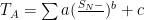
Grrr. Goddamn WordPress latex interface. OK, I’ll present the equations it screwed up above without the latex translation attempt.
T_a = \sum [ a (\frac{S_N – }{}^b + c ]
is the proposed fit without the cosine term, using a normalized, dimensionless sunspot anomaly as the single variable in the rate equation, not the absolute number. is the mean sunspot number averaged of the entire interval. One expects this to be roughly halfway between 0 and the sunspot peak, so normalizing with respect to it converts the sunspot number from being something in the tens to hundreds to something ranging from roughly -1 to +1, with rare excursions above +1. One could just renormalize S_N/ to accomplish the same thing and make the range 0 to 2+, but then one would almost certainly alter part of the possible meaning of c. Given the sorta-Gaussian shape of the solar cycle, there are probably even better transforms — deviation from the a local “mean” solar cycle, for example — but this is worth trying and should accomplish most of what the “a” parameter is accomplishing now in the fit up above.
rgb
http://www.elsideron.com/wuwt_ssn_study
As you can see, despite the noise added to the SSN is so low that ti would not even affect the published monthly SSN values, doing the reconstruction with the new SSN values instead of the strictly published provides strikingly different results. That’s why this reconstruction has absolutely zero value.
Broken link, Nylo. I agree, mostly, but I have to say I’m surprised. The sum of the cosine of a random number should rapidly converge to zero, and d is a small number to start with. It should make the fit bounce around a bit initially and by the 100th month cease to be relevant, much less than 10% of the total, should it not?
Either way, I agree that the term is utterly meaningless and needs to go because it is not robust to the error in the data — it is just a transform of noise. Not that the whole fit isn’t Nikolai and Zeller style numerology in the first place… but there are terms (as I showed) that one COULD turn into a POSSIBLY reasonable model.
rgb
You should have Climate Audit / Steve McIntyre analyze & critique this analysis.
Wouldn’t THAT be a nice change of pace in an us-versus-them arena in which “sides” are so clearly defined & maintained with great effort….
…that is…seeing people on the ‘same side’ actively work to ensure the validity & objectivity of the analyses & conclusions they reach rather than just apply the analytical criterion of, “Oh! That agrees with my outlook, so I’ll accept it without any objective critical evaluation.”
E.G., note “wsbriggs” observation May 3 at 4:28 am, above.
Once again, the great quality of the comments is on display at WUWT. Thanks to all who’ve convinced me to take the original post with less than a grain of salt.
Suggestion: Instead of removing the post, add an update to it indicating that those readers of this blog who have a good understanding of the math involved have found serious fault with the analysis. That would serve two purposes: 1) It would confirm the policy of not deleting posts/comments, and 2) It’s retention, along with the update, would serve as a cautionary note for others who are considering posting articles under the new policy, since their efforts will be on display for the duration of WUWT, hopefully a very long time.
Besides, in its own way, the article, taken together with the comments, was educational, just not in the manner the author intended.
Cosine? Really?
So, somehow it fits to the highly manipulated global temperature series.
When I see something that matches the un-adjusted raw temp records rather than the UN-adjusted temp record I might get interested.
As soon as I see data with the average global temps from 1930-40 way below current, I just ignore .
Thomas says:
May 3, 2013 at 3:57 am
What result do you get if you use the first half of the data to estimate all your parameters and the second half as a control?
You’ll end up with garbage
#########################################
even if you didnt the deeper problem with this and with all solar analysis that works with
“spot numbers” is that they are diemensionaly incorrect.
our climate system doesnt “see” spots, it sees watts.
So if you have temperature on the left hand side you better have units on the right hand side that can be related to temperature via known laws of physics, otherwise, even if your curve fit is perfect, it’s meaningless.
rgbatduke, try plotting the formula proposed by the author, instead of against the SSN values published by NASA, against a SSN varying in 0.1 steps, between 0 and 30, ignoring the sumatories and “e”. What you will get is what the nonsensical formula says that a particular month with that SSN contributes to the trend in temperatures. I have plotted it for you:
http://www.elsideron.com/wuwt_ssn_study/Monthly_increment_by_SSN.PNG
As you can see, the SSN “magnitude” doesn’t really matter. I plotted until SSN=30 but you can continue to 200 if you want, very little changes. A month with SSN=0.1 can contribute much more (increasing temperatures by 0.007C) than a month with SSN=29.8 (which reduces them by -0.011C). And the reverse is true for sunspot numbers 0.3 and 29.4.
So how come the author gets a result that comes close to what has happened with the temperatures? Just by extremely carefully playing with “a” parameter until, by absolutely pure chance, the results of the cosine of its multiplication by the published SSN more or less matches the ups and downs of real temperatures. It is not so difficult to achieve if you use an “a” really big as he does and start changing it in tiny ammounts until you get what you want, which he does. He probably tried several thousands of possible values of “a” until he found one that produced a result which was “good enough” for him. Then he adds the other terms which just create an escalator roughly matching the overall trend and voilà. See the escalator below in green (his formula except for removing the cosine (cosine=0):
http://www.elsideron.com/wuwt_ssn_study/No_cosine.PNG
A caution for careful, sensible readers:
In their haste to ignorantly &/or deceptively (and falsely) paint the cosine integral as noise, some commentators are failing to recognize that the term is simply pointing to scaling changepoints in the sunspot record. An infinite number of other summaries can be designed to capture the same nonrandom changepoints. A subset of such summaries are physically meaningful. I suggest more sobriety. Salvador’s cosine term may be physically meaningless, but there’s an important learning opportunity here for anyone patient & careful enough to deeply understand and appreciate exactly why the cosine integral’s changepoints are timed as they are.
__
A light-humored peripheral note for those concerned about the number of model parameters:
Please be fair in your comparisons.
Tell us how many parameters there are in each of the IPCC models.
(Let’s see if that’s a long list of big numbers.)
The yearly average temps for the earth fit a cosine curve nicely. The northern hemisphere is more land-covered and varies greatly in seasonal temperature variations. The southern hemisphere has much lower variations, due to greater ocean coverage. So when they are “averaged”, the northern hemisphere creates a larger seasonal change, and is going to force a positive anomaly in the May – Sept months, and force a negative one in the Nov – March months.
Looks like a cosine to me.
Clearly the progressives will begin to postulate that CO2 drives solar cycles.
Paul Vaughan, “there’s an important learning opportunity here for anyone patient & careful enough to deeply understand and appreciate exactly why the cosine integral’s changepoints are timed as they are“.
There’s nothing to understand other than this is an exercise of curve fitting with total disregard as to the significance of the paremeters. I already demonstrated that, many replies ago, by adding a tiny, imperceptible noise to the SSN and seeing what happens with the reconstruction. The formula is so sensible to tiny variations of SSN that the results often no longer had any resemblance to the original. The author’s method to choose the “a” parameter resembles putting a billion monkeys in front of typewriters until one writes “IPCC=SHIT”. He has then picked that “monkey” (that “a” value) and presented it to us as the great monkey of ultimate wisdom.
The big difference with the IPCC models is that IPCC parameters are at least based on something physical. I won’t dispute that they are as well examples of curve fitting, of course they are and that’s why I don’t believe in any of them, those parameters are chosen in preference to others as plausible as them just because they give the desired results. But they have a base. They can be explained, they can be defended, whereas “a” cannot. It is the most absolute crap.
thingodonta says:
May 3, 2013 at 3:49 am
You can’t tax sunspots.
Wanna bet!
It is obvious from these data that Congress must increase its solar spending. We just aren’t spending enough on the sun.
I would also like to add that curve-fitting is how Calculus was derived.
So there is a history of getting data that is not well-understood, and finding mathematical formulas that describe it, before you understand how the variables are producing the resultant data.
@ Nylo (May 3, 2013 at 8:53 am)
My patience for your ignorance &/or deception has expired. Do not address me again.
REPLY: Mr. Vaughn. This isn’t your blog, and if people want to write posts to you, it is my call as to whether to allow them or not, not yours.
In this case I agree with Nylo. You would do well to learn some manners – Anthony
Its interesting that the Sunspot Number and temperature anomaly correlation is there at all, I attempted to break the temperature anomaly down into individual temperature records and found that the correlation exists there as well, on the Northern Hemisphere there is a lag between solar activity and temperature that varies with Latitude (did you know that?). Depending on the latitude where the temperature reading is from, there is a Lag of up to 3 months between solar activity and temperature, this would be due to seasonal variation and what state of activity the sun was in.
http://thetempestspark.wordpress.com/2013/02/15/average-november-sunspot-number-and-february-minimum-temperature-1875-2012/
This raises an important question for me, As the global temperature anomaly is from land based stations and the majority of earths land mass is on the northern hemisphere, Is the temperature anomaly showing the seasonal variation of the Northern Hemispheres exposure to solar activity through stronger and weaker solar activity?
If it is, then it basically means that the Global temperature anomaly is not an accurate measurement of earths temperature “evenly distributed globally”, but is an anomaly that represents seasonal variation of Earths exposure to solar activity through stronger and weaker solar activity over time.
The exposition is unclear to me. What are the limits of the summation? From the description, it seems as though the predictor is a recursive one, but perhaps that’s not what you meant. This is interesting, but a clarification is needed, in my view.
It might help if you used MathJax.
Thanks Nylo for a clear, elegant, and ultimately very convincing reminder that curve fitting has very little to do with science. I was first intrigued and taken in by the “correlation” illustrated in this post, but your noise sensitivity analysis unambiguously demonstrates that this curve fitting process is a completely artificial and meaningless exercise in noise fitting. I am a bit ticked at my initial interest and poor scientific judgment (big big difference between correlation and causation), but you set me straight (and I hope others). Again many thanks.
I still prefer my old leprechaun fit: http://rankexploits.com/musings/2009/you-can%E2%80%99t-make-this-stuff-up-ii/
I managed to get an r^2 of 0.73 with just one parameter!
I don’t see Salvador’s model as being any more or less valid that the current crop of GCMs. In fact they are quite similar in that they each have many ‘tunable’ parameters that permit curve fitting to the historical temperature profile one chooses to match. They are all just curve fitting. At least R.J. is honest in not claiming that his parameters stand for some as yet undetermined physical parameter that they ‘think’ might approximate the value used. And, he doesn’t throw in a few million lines of code in order to justify development costs that in reality, like his cosine term, just add a lot of noise and are negated by the tunable parameters.
In other words, at least to me, his model is no more nor no less valid in predicting tomorrow’s climate that any of the current crop of GCMs that we’ve probably spent billions developing. Besides, “the fact of the matter is” (Lord I hate that phrase) is that it appears to do great job of matching the temperature record chosen.
E=MC2 is just curve fitting!
Interestingly, I did a max temp vs bright sunshine correlation for the Central UK which predicted that the max temp and bright sunshine would end in 2010 (NothingSettledNothingCertain.com).
Your first graph: it is the fit of your prediction to the actual, I gather. The linear relationship is then the how your prediction X 1.0024 the actual, i.e. your prediction has a 2.4% underestimation of the temp as measured by GISTemp data. This linear difference is perhaps similar to my 0.1C/century that was left out of my sunshine + PDO/AMO heat release/heat retention cycles. I thought land use OR CO2 could explain it.
Try plotting the deviation from prediction vs time and see if there is a pattern that matches the PDO/AMO signal.
Joe Crawford:
Your post at May 3, 2013 at 10:30 am concludes saying
OK, I will accept that.
No model is a perfect emulation of anything. Every model is assessed by its usefulness.
What use does this model have?
1.
The model cannot assist understanding of climate behaviour.
It is a curve fit using purely arbitrary variables which represent no known physical parameters to obtain agreement between sun spots and one climate indicator. Adjusting one of the parameters will alter the indicated relationship, but that adjustment indicates nothing about climate because the parameter has no relationship to anything in climate.
2.
The model has no predictive ability.
The model relates sun spots to one climate variable. Assuming it does indicate a true relationship between them (which is doubtful) then neither of them can be predicted so there is no available prediction of one of them which is necessary for the model to predict the other.
Simply, the model is worthless: it is not even wrong.
Richard
First, Mr. Salvador, you have done a mountain of work. Several comments on it, in no particular order.
I fear that there is no way to sugar-coat my opinion. I see this as a meaningless curve fitting exercise. Why do I say that? I’ve read countless papers, and done countless analyses of this type myself. As with most parts of my life, I’ve developed some rules of thumb for identifying curve fitting. For me, the tell-tale indications of meaningless curve fitting are:
1. A large number of tunable parameters , in this case five (a, b, c, e, and f). For those unaware of the importance of this issue, let me quote from Freeman Dyson:
The problem is that (as in this case) if you are given free choice of any mathematical expression, combined with five tunable parameters, you can truly make the elephant wriggle his trunk in the exact shape of the historical temperature record … and regarding that, I can only bring you the “bad news” that Dyson brought back to his students. Your results mean nothing.
As someone commented above, to be fair I should note that climate models do the same thing, they have many tunable parameters … but then I don’t think they’re worth a bucket of warm spit for forecasting either … or for hind-casting, for that matter.
2. Ultra-high precision required in specifying the parameters. If you need more significant digits for your parameters than your data contains, you are in very dangerous territory.
3. Lack of an underlying physical theory. While not a fatal objection, it certainly applies to such convoluted methods as we see above. Let me give an example of why lack of a physical theory is not a fatal objection. It seems clear that the slow decay in the concentration of an injected pulse of CO2 (or other gas) into the atmosphere follows an exponential form. We do not understand all of the myriad pathways that carbon takes wandering around this marvelous planet, so we don’t have a complete unifying theory about why the average of all of those carbon pathways comes out to have an exponential form … but there it is in the records. So in that case, the assumption of exponential decay with a single time parameter may be justified despite the lack of a complete theory.
In the current instance, however, we have nothing to underly the convoluted, counter-intuitive, claimed mathematical relationship. In such a case, the lack of a physical theory looms large.
4. An “over-good” fit. Things in the real climate are messy. There’s a lot of what climate scientists call “noise” in the data, which is a technical term meaning “we don’t have a clue”. A result as good as this one is far too tight a fit to the historical data to be believable. A fit as good as the one shown would imply that other than sunspots, almost nothing affects the global temperature … very doubtful.
5. Bad units. As Steven Mosher noted above, you have sunspots on one side of the equation, and temperature on the other. Although in some circumstances this is handled by introducing a constant “C” having some kind of imaginary units to convert one to the other, in this case we end up with degrees per sunspot number to the nth power … bad sign.
6. Small data sets. Not an issue in this case, but see e.g. Nikolov and Zeller for some high-quality curve fitting on a data set of a dozen or so.
7. Hyper-sensitivity to small changes in data. As Nylo points out above, if you add a tiny random value to the data, the formula gives a hugely different result. Any formula that sensitive to the random fluctuations of the data is over-specified.
8. Lack of testing using withheld data. As several commenters have noted, cut the data in half, and derive your parameters in the same manner using solely the first half of the data … then use those parameters to project the results to the second half. I suspect you’ll be shocked.
Those are my rules of thumb for identifying what I describe as meaningless curve fitting exercises, Mr. Salvador. And I fear that your exposition above fits all of them but one, you used large data sets. As a result, and sadly, I have no hesitation in identifying your work as not being of value.
Now, Dr. Robert Brown, who posts as rgbatduke in his comments above and whose science-fu is very strong, said that if you dropped the strange cosine stuff that what remained might make sense. Unfortunately, wordpress ate the important parts of his equations, so I’m not clear what he meant, I’ll have to derive the math myself. But in general, I fear that your claimed results are totally spurious.
Finally, someone said that this paper should be retracted. I couldn’t disagree more, this is science in action. I have no problem with bad science being put up and shot down here. I’ve seen some of my own go down in flames.
However, I did like the thought of putting a comment up at the top noting the objections of some commenters, let me consider that. In a way it constitutes some kind of peer review, with the obvious pluses and minuses.
Perhaps just a brief note at the top that there are objections, with links to salient comments, at the top of the post … suggestions welcome, although they may be ignored …
w.
Nylo is absolutely correct.
If one simply plots the two components of the equation separately, one can see that the cumulative sum of the cosines provides virtually the entire fit to the variation of the temperature anomaly, while the cumulative sum of the powers is pretty close to a straight line. The function cos(148.4258*x) goes through a complete cycle for every change in x of magnitude 2*pi/148.4258 or 0.0423. In effect, it generates “random” values basically matching the residuals from a linear fit of the cumulative sum of the powers.
There is no viable predictive value to the fit.
TA= d*[Σcos(a*SN)-Σb*SN^c]+e from month 1 to the present
Is there a typo in that equation? cos(a*SN) with a = appx 148 is peculiar. Also, the sum of those numbers from month 1 to present is a single number — to what does it get compared?
How about some estimated standard errors on those parameter estimates, and fewer claimed significant figures?
It looks like totally uninformed post-hoc model fitting, but perhaps a clearer presentation would clear that up.
The problem is that you can build a formula giving you any curve from zny input. For example I can build a formula giving the level of dow jones index from the temperature in Arkansas. That is curve fitting… the formula works for the period it was built for…but it does not mean temperature and dow jones are linked…and it will fail miserably to predict the future.
son of mulder says:
May 3, 2013 at 4:19 am
“And what was Newton’s physical explanation for the parameter ^2 in the gravitational inverse square law?”
Divergence of the force is zero – empty space is neither a source nor a sink for gravity. That leads ineluctably to a 1/r^2 dependence.
There is nowhere near the tight correlation shown in that top graph. There is far more to it than that and even publishing this article is a disgrace. Here is SSN and CET (no not what the article compared). https://sites.google.com/site/ralulacet/sunspots/sunspots-and-cet
I agree with Willis Eschenbach, but isn’t the point being made by R.J. Salvador’s that it is possible to build a correlation between sunspot numbers this way? as an example and in regard to how Anthropogenic Global warming proponents use statistical methods to build their charts, otherwise why would R.J. Salvador admit to the process and provide the method.
I’m not a statistician, as an engineer (studying science to improve my understanding) I use precise values at a precise point in time to measure what the values are doing at any precise interval, where they are and what the relationship is between these values and their upper and lower limits. If I were to use curve fitting to get a desired result it could result in death or injury.
Having said that, do you think that this chart is curve fitting?
http://thetempestspark.wordpress.com/2013/02/15/average-november-sunspot-number-and-february-minimum-temperature-1875-2012/
@ HenryP:
Read your links. Couple of comments:
Not seeing the need for a religious reference at all. You don’t have much religion in the article anyway, and it mostly just distracts.
It looks like you are leaning toward a ‘cold catastrophe’ expectation. It isn’t warranted. There is NO global shortage of food, nor shortage of excess growing capacity. Farming is already growing by leaps in Brazil and Africa. Furthermore, about 40% of US corn goes into gas tanks. We can massively increase food supply by not feeding it to cars. (Gasoline can be made from coal, as can alcohol, for centuries to come if needed – but it won’t be, as we are awash in natural gas.)
There are also massive amounts of grains fed to animals. In any real “food crisis” we can eat the grains ourselves instead. It takes about 10 lbs of grain to make one lb of beef, and about 3 pounds to make a pound of pork or chicken. As the meat is mostly water, and the grain is dry, the relative ‘food content’ of each pound is higher in the grain as well. (I can easily eat a one pound steak, but one cup of rice makes more rice than I can possibly eat in one meal… It takes about 1 dry pound of food per person per day, or 1/3 lb / meal, and you are well fed.)
At present, the global problem is over production. (Germany is dumping rye anywhere it can…)
Finally, we can easily swap to more cold tolerant crops. Oats and Barley, for example, grow in just barely defrosted dirt. The big issue isn’t cold, it’s water. Both too much and too little, and wind blowing down crops. (That’s why potatoes work better than wheat in bad times…)
So yes, it’s going to get a bit colder. Yes, far north farmers will have a harder time of it, but no, it won’t matter on a global scale.
http://chiefio.wordpress.com/2013/01/11/grains-and-why-food-will-stay-plentiful/
@Paul Vaughan –
I suspect quite a few regular posters here are fed up with YOUR ignorance/deception.
@thingodonta/kelvin vaughan – Just watch the kleptocrats find a way to tax sunsposts – and transits of Mercury – and previously undiscovered comets and asteroids – and supernovas in galaxies 10 billion light years away.
@Nylo – don’t let the alarmies discourage you.
The random “noise” assumptions made by several critics fail:
http://img32.imageshack.us/img32/347/rx22anim.gif
http://tallbloke.files.wordpress.com/2013/03/scd_sst_q.png
http://img201.imageshack.us/img201/4995/sunspotarea.png
http://imageshack.us/a/img692/3756/c1a6mo.gif
Suggestion: Take some weeks &/or months to more deeply understand and appreciate exactly what Salvador has captured (whether by accidental fluke or trick awareness).
Personally, I think the cosine term is an unphysical kluge. But, the broader point that the area under the sunspot curves was generally increasing in the time of increasing temperature is important. It probably explains the overall trend, even as variability is introduced by the system response.
Bart says:
May 3, 2013 at 1:20 pm
son of mulder says:
May 3, 2013 at 4:19 am
“And what was Newton’s physical explanation for the parameter ^2 in the gravitational inverse square law?”
Divergence of the force is zero – empty space is neither a source nor a sink for gravity. That leads ineluctably to a 1/r^2 dependence.
While true Bart, that isn’t very helpful to people with low level math.
More simply, the relationship of an expanding sphere’s surface area to it’s radius is inverse square.
Thus if the medium itself is frictionless to the energy (Bart’s “neither a source nor sink”) you would expect gravity to be inverse square.
And let’s not forget that Newton was wrong.
My best guess at where critics are going fatally wrong with their “random” noise assumptions:
Failure to recognize that amplitude change temporal autocorrelation must necessarily shift phase with solar cycle deceleration (SCD). Such a failure would lead to a further failure to recognize the potential to lace an average harmonic through the manifold and (either brilliantly or haphazardly, depending on whether it was conscious or not) yank out a crude alias of the shifting anharmonic framework that gets considerably sharpened up (in central limit) by integration.
I wouldn’t expect that anyone here would realize the preceding.
Note for the few — if any — who are willing to work patiently & carefully on this to arrive at a more lucid level of awareness: I’ve done the diagnostics on this and Salvador has indeed sampled a proxy for SCD (whether accidentally or intentionally).
Sparks says:
May 3, 2013 at 10:41 am
E=MC2 was derived using Newtonian physics before Einstein was even born, by Weiss.
The thought experiment was a train with perfectly reflecting mirrors at both ends of the car, tangential to the direction of travel. It’s 30+ years since I read it so it’s a bit fuzzy, sorry.
Gerrit, Jan Pompe and I did a bit of curve fitting ourselves before he died.
What we tried to do was build a model of our climate as an LCR filter with TSR as input and temperature as output and managed to get a fair correlation. My contribution was small, though I think I suggested a transistor effect for something.
I’ll try to retrieve it for anyone who’s interested. Gmail’s great for the amount of back data you can have.
DaveE.
I’ll just throw this out there; RJ, I don’t know who you are, but you either are presenting this as a legitimate discovery or you are presenting this as bait.
It remains to be seen if the ‘alarmist’ websites point to this article as an example of the gullibility of the people who frequent this site.
Either way; the comments prove that there is a diverse base of knowledgeable people commenting on the articles presented here. And they sniffed it out pretty quick.
If you truly did believe you had found something; congratulations. You did. You learned that curve fitting is an exorcise akin to the reading of tea leaves. I believe Thomas Edison found 10,000 ways NOT to make a light bulb before he figured out how TO make one.
If you wrote this as a way to demonstrate how gullible us rubes are, over here at WUWT, then I suggest you take your findings to the ‘alarmist’ websites, and let them know that not everyone who questions the alarm bell of CAGW is an idiot or a paid shill. You might also point out to them that curve fitting is as far from science as a rain dance is from meteorology. You aren’t the first person to employ the method in climate science, and right now a lot of it passes for GCMs.
Or, you can go back and point out that it got published at all, pretend we didn’t notice the fallacy of your work, and also pretend that you aren’t part of a cult. Climate science is science. The alarmism surrounding climate science right now is not science, and a lot of that alarmism masquerades as science. Real scientists are and will be hurt by this charade. And worse; if real scientists actually do, in some future period, find something that should truly alarm the people living on this planet, it is likely that these charlatans will have cost them their credibility in advance. Instead of saving the planet, these fools could very likely doom the future of mankind.
As I said; if you truly thought you found something, congratulations, you did. If you are a baiter, congratulations, you found something as well. If you are too small to learn from it; I guess your fate was probably decided well before you ever wrote the article.
cos(a*SN) with a=148 is essentially a (bad) pseudorandom number generator. Even small changes in SN (which is measured to 1 decimal place) give large changes in cos(a*SN). So Σcos(a*SN) is a random walk, the shape of which is controlled by a.
Σb*SN^c is monotonic, it provided the trend for the wiggles in Σcos(a*SN).
This is simply a curve fitting exercise, with no physical meaning.
Any idea what John Cook says about this?
Livingston and Penn wrote a paper: “Sunspots may vanish by 2015″ that was posted on this blog. What happens to the global temperature anomaly if sunspots do vanish by 2015?
Mooloo says:
May 3, 2013 at 4:47 pm
“And let’s not forget that Newton was wrong.”
He was not wrong, he was incomplete. In a static situation with no angular momentum, the acceleration with respect to proper time is still Newton’s formula.
David A. Evans says:
May 3, 2013 at 5:04 pm
E = mc^2 follows directly from the postulate that the speed of light is constant in all reference frames, so it is not a curve fit. As Newtonian physics has nothing to say about the invariance of the speed of light, I do not see how it could be derived from it. But, the relationship was derived by Henri Poincare before, or at least contemporaneous with, Einstein. It is the outcome of calculating the energy using the Lorentz Transformation, so Lorentz could have derived it if he had been attuned to do so. Larmor and Fitzgerald probably could have, too.
“What we tried to do was build a model of our climate as an LCR filter with TSR as input and temperature as output and managed to get a fair correlation.”
It sounds reasonable to me. An oscillatory response driven by outside forcing akin to that provided by the progressively strengthening solar cycle is basically what the temperature series looks like to me.
E.M. Smith says
http://wattsupwiththat.com/2013/05/03/sunspot-cycle-and-the-global-temperature-change-anomaly/#comment-1296527
Henry says
I do appreciate your comment and the criticism. As I said : the biblical references were only added in because I want to reach a Christian/Judaic audience. Just ignore that.
I determined in three different ways that the beginning of warming started around 1951 and the cooling part of the cycle started around 1995. This is looking at energy-in.
Average temp. on earth will lag a bit. But, clearly you can see that the trend is negative for the past 12 years:
http://www.woodfortrees.org/plot/hadcrut4gl/from:1987/to:2014/plot/hadcrut4gl/from:2002/to:2014/trend/plot/hadcrut3gl/from:1987/to:2014/plot/hadcrut3gl/from:2002/to:2014/trend/plot/rss/from:1987/to:2013/plot/rss/from:2002/to:2013/trend/plot/hadsst2gl/from:1987/to:2014/plot/hadsst2gl/from:2002/to:2014/trend/plot/hadcrut4gl/from:1987/to:2002/trend/plot/hadcrut3gl/from:1987/to:2002/trend/plot/hadsst2gl/from:1987/to:2002/trend/plot/rss/from:1987/to:2002/trend
From the above simple compilation of linear trends in these 4 major global data sets, you can also see that before 2000 we were still warming and that after 2000 we started cooling….
Obviously this cooling will continue. We are on a 88 year cycle, so to calculate where we are is simple: 2013 – 88 = 1925.
Now I said, and I quote: “So, a natural consequence of global cooling is that at the higher latitudes it will become both cooler and drier.”
I remembered something of the 1930’s dust bowls and looked it up for you. We are not that many years away from this. Check this study:
http://www.ldeo.columbia.edu/res/div/ocp/drought/dust_storms.shtml
To quote from the above study:
“The Dust Bowl drought of the 1930s was one of the worst environmental disasters of the Twentieth Century anywhere in the world. Three million people left their farms on the Great Plains during the drought and half a million migrated to other states, almost all to the West”
end quote
That looks pretty serious to me. Now I never said things will become catastrophic as that, but due to the droughts it could become a bit challenging in the years ahead? Better to know these things beforehand? Remember, there are now so many more people looking for food than we had in the 1930’s.
As far as this post is concerned, I am disgusted that “R J Salvadore” does not even bother to show up to defend his work. I think people like that should not be allowed to post here at all. I have to conclude that he is just a phantom writer trying to confuse issues for us and trying to lead us in the wrong directions. We all know who he is, don’t we? My conclusion was that he suffers from a multi personality disorder. (in the olden days they would say:possessed by the devil. In this case we would say in dutch: he has a “plaaggeest”. (teasing spirit)
Forget about all this nonsense in this post. To fish out where we are with the sun, you only have to look at direct the measurements, like average daily data from maximum temperatures, converted to yearly average data. I have done it all for you. You can just repeat it.
http://blogs.24.com/henryp/2013/02/21/henrys-pool-tables-on-global-warmingcooling/
Henry said
you only have to look at direct the measurements, like average daily data from maximum temperatures, converted to yearly average data.
Henry says
sorry that should have been:
you only have to look at direct measurements, like daily data from maximum temperatures, converted to monthly average data, converted to yearly average data.
Re: Dr. Svalgaard
Data on his charts
http://www.leif.org/research/TSI-SORCE-Latest.png
http://www.leif.org/research/TSI-SORCE-2008-now.png
use to get updated daily with no more than day or two delay
It looks that the last updates was for 10th of April (jugging by F10.7 flux)
There is also a paper
http://www.leif.org/research/Synoptic-Observations.ppt dated 27 April
I hope that Dr. S. is well, his absence from the solar threads is very much missed.
five parameter and an arbitrary choice of mathematical functions…
Sorry to say it demonstrate nothing. And you knew from the beginning that a crude sunspot number has followed global mean temperature in the past…
But you can do several test..first truncate the data find out new parameters and see predictions
Try to do the same analysis using something different from sunspot number…and so on…
Or wait 20 years to see if predictions are still valid!!
some other did the same job it with fourier analysis, the principle is the same..if there is no physics it is just fitting curves..somethings you can always do if you use enough parameters.
vukcevic:
At May 4, 2013 at 1:35 am you say
I write to draw attention to your “hope”.
A few days ago I made a WUWT post which noted his absence, said he is a valued member of the ‘WUWT community’ and asked if anybody knew he is OK. Nobody has responded.
I again ask if anybody can confirm that Lief Svalgaard is alright.
The lack of news is becoming concerning to you, to me, and feel sure to many others in the ‘WUWT community’.
Richard
I did a much cruder version of this correlation in 1987 when I was working in ag chemical research. I got a similar correlation coefficient. I found that the correlation improved dramatically when the sunspot count was correlated with the temperature three years later, my reasoning being that any effect would be reflected after one atmospheric mixing. That sound reasonable?
henry@richard, vukcevic
come on you guys.
You honestly had not figured out yet that R.J. Salvadore is Dr. S?
He is a real Jeckyl and Hyde,
so he is hiding
“Bart says:
May 3, 2013 at 1:20 pm
Divergence of the force is zero – empty space is neither a source nor a sink for gravity. That leads ineluctably to a 1/r^2 dependence.”
That’s not a physical explaination, purely an assumption that the mysterious gravity diminishes as a sphere’s area increases with r as R^2.
It does not physically explain how the force is transferred instantaneously from one mass to another, so it’s no different in principle to what R.J. Salvador is doing ie see a pattern but not know the possible physical mechanism. But it is quite reasonable to create a scientific hypothesis in this way, test it and move on as appropriate.
Henry
No sane person working in any kind of science would quote parameters withs ao many decimal places
a= 148.425811533409
b= 0.00022670169089817989
c= 1.3299372454954419
e= -0.011857962851469542
f= -0.25878555224841393
unless it is a send-up.
E=MC2 is just curve fitting!
…speaks ignorance so abysmal that it would take a very long rope to even reach down to offer you a leg up.
Indeed, understanding the difference between an amazingly well-founded, empirically supported theory and “just curve fitting” is precisely what the debate is about. Nylo, I agree with everything you are saying (again). I have to admit that I am a bit surprised that they were able to find a way of scaling the integral of a cosine of what amounts to a cosine squared to fit anything at all (especially with a large multiplier) but I’ll take your word for it. Either way, the term is clearly totally bullshit.
There are, sadly, a few people who love to fit curves to data and then pretend that the result has extrapolative predictive power. If you’re going to play this game, you might as well not screw around with crippled bases. Build a neural net. At least then your basis is generalized nonlinear function approximator capable of resolving nontrivial multivariate correlations.
Anything else is kid’s stuff. Henry P fits a second order polynomial to predict the future. This paper fits a bizarre, meaningless function with meaningless parameters. Neural nets yield meaningless fits in the specific sense that the weights cannot be connected back to anything causal, but damn! They can actually sometimes manage some pretty damn good predictions of highly multivariate, nonlinear probability distributions in predictive models. The only way one can — sometimes — beat them (and the other related Bayesian methods) is with a really, really solid, physically motivated model fit/trained by an expert statistician.
Of course, building a predictive NN requires following rigorous rules. One has to regulate the power of the (potentially vastly overcomplete) representation by limiting the number of hidden layer neurons to the minimum that can capture the data without overtraining. One has to split available input data in to training and trial, to verify that the trained net has at least some plausible predictive power on data outside the training set. And in the end, one is still susceptible to black swan syndrome and/or omitted variable syndrome (and to simple errors or noise in the building process).
Building good predictive models is not a game for the amateur. Seriously. Given a choice between ordinary physics and high end statistics, it isn’t clear which one is more difficult. Statistical mechanics is one of the most difficult subjects in the world, and climate science is technically, arguably, THE most difficult subdiscipline of statistical mechanics. So give this sort of thing a rest, is my advice. Post hoc ergo propter hoc is a logical fallacy in the first place, and what value it has is easily abused.
rgb
rgb says
Henry P fits a second order polynomial to predict the future.
Henry says
No I did not.
I refer to the 4 results for the speed of the drop in daily maximum temperatures (average, global) on the bottom of the first table here:
http://blogs.24.com/henryp/2013/02/21/henrys-pool-tables-on-global-warmingcooling/
When you set the speed of warming/cooling out against time, indeed, the binomial for the drop in the speed of daily maximum temperatures, had a correlation of 0.997
For any statistician that is a dream come true (on his random sample)
But I figured in the end that would drop us into an ice age quite quickly…..
That shows you: even with very high correlation you are still not save with a curve fit of 99.7% correlation…apparently….
In the end I found that a sine wave would also be a good fit and if you put the wavelength at around 88 years, the fit looks reasonably good, though I did not do a correlation. (don’t know how to to do that if Excel does not know that either)
http://blogs.24.com/henryp/2012/10/02/best-sine-wave-fit-for-the-drop-in-global-maximum-temperatures/
Anyway, either way, I also used two other methods to determine the dates of ca. 1951 and 1995 as turning points on my a-c wave. Which is making me confident in estimating that the next turning point (from cooling to warming) will be around 2040, give or take a few years (of my error)
” vukcevic says:
May 4, 2013 at 4:47 am
Henry
No sane person working in any kind of science would quote parameters withs ao many decimal places”
What about the fine structure constant 7.2973525698(24)×10−3 ?
http://en.wikipedia.org/wiki/Fine-structure_constant
Thanks for the comments. Let me address some of the objections being made to the correlation.
The main one is that the correlation has no physical significance. I disagree. The correlation’s two terms each measure a different physical phenomena and its accumulated effect on temperature over time.
The b*SN^C term measures the accumulated effect of the total solar cycle over time. It has been proposed by others that this involves cloud formation through a mechanism involving blocking cosmic rays.
The Cos(a*SN) term measures the accumulated effect of sunspot oscillations within a cycle. I believe that is why the frequency associated with this term is high. It is a sunspot change frequency. Each sunspot cycle is different not just in terms of magnitude and length but also when the sunspots appear and disappear. The mechanism that ties it to a temperature change on earth I suspect is also related to a cloud forming mechanism. Some have suggested that this term is just an alias for a more complex set of curves. That maybe true. I chose to stay with the simplest equation that matched the data.
Some have suggested that the equation is only valid after a number of summations. The least squares test is evaluated over the 1598 summation equations of the data points. The equation is as valid or invalid for the first data point in January of 1880 as the last data point in February of 2013.
And I apologize for the typo in listing the parameters. ( e is d and f is e)
I think quite to the opposite of some here. I think the post by RJ Salvador is intended to prove to the Alarmists that this site is not full of a bunch of dunces who just jump on anything that goes against CAGW.
As illustrated by the responses, the WUWT community does not just accept any old thing that comes down the pipe. The WUWT community is as likely to tear apart reports that agree with their position that CO2 is not the culprit, as they are at tearing apart the crap that is passed off as science that claims CO2 is the driver of climate change.
All well and good but what I’d like to see is someone predict the next Heinrich Event which will probably kick us firmly into the next glaciation. My guess is 4000 years.
vukcevic says
No sane person working in any kind of science would quote parameters with so many decimal places
henry @vukcevic,
I am not saying he is insane. I do think he got very tired at beating us down until now, (recently?) he must have come to a conversion (to now being a full blown skeptic).
Perhaps he has now realized that we are going to cool down in the next 3 decades and that no amount of carbon dioxide in the air will stop that from happening. But, now, he does not want to come out of the closet, yet, so to speak. He is too afraid.. He is is feeling guilt…. He needs our help. Let us quote him this verse from the bible:
When I kept things to myself,
I felt weak deep inside me. I moaned all day long.
My strength was gone as in the summer heat
Then I confessed my sins to you
I did not hide my guilt
I said: I will confess my sins to the Lord
And you forgave my guilt.
Finally we have proof that Man Made Global Climate Change is not only affecting Earth, but it is clearly affecting the Sun
The fact that Global Temp appears to lag Sunspot Activity helps reinforce that Ancient CO2 levels Lagged Temp. yet still were the cause of the Temp. rise.
It all makes sense now.
Why this does strike me as an example of over-fit curve fitting, I do think the insistence on a physical mechanism is one of the weaknesses of climate science and modern science in general.
Climate may be considered a Function of what we Know and what we don’t known – the Unknown. Mathematically this might be expressed as:
C = F(K,U)
Given C and K, solve for F and U.
So, if we limit ourselves to only those terms that have a known or hypothetical mechanism, we are unlikely to arrive at the correct answer. This has been very amply demonstrated by the current climate models, which have gone off the rails post 2000, and demonstrates that they are also nothing more than curve fitting.
Paul Vaughan says:
May 3, 2013 at 4:51 pm
Realize it? Paul, I can’t even understand it. “Lace an average harmonic through …”? “Crude alias of the anharmonic framework …”?? “Amplitude change temporal autocorrelation …”???
‘Fraid I’ll have to pass, my friend.
w.
ferd berple says:
May 4, 2013 at 8:17 am
Thanks, ferd. In science there is no “insistence on a physical mechanism”. As I pointed out above, such a lack is a problem but not a deal-killer. I had said:
In this case, we have a very, very strange mathematical relationship with no known physical basis. In such a case, the lack of a possible mechanism becomes a more significant issue.
w.
R A Salvador @ May 4, 2013 at 7:31 am
The Cos(a*SN) term measures the accumulated effect of sunspot oscillations within a cycle. I believe that is why the frequency associated with this term is high. It is a sunspot change frequency. Each sunspot cycle is different not just in terms of magnitude and length but also when the sunspots appear and disappear.
This is sheer fantasy.
For a particular month, Cos(a*SN) is the added contribution from the sunspot number for that month. Have you bothered to see what those values look like? Note that the sunspot numbers are all single decimal values. As an example, suppose we calculate the values from the Cos term for the values of SN from 50.0 to 51.0 (or pick any other range – the effect is the same) :
50.0 0.66093757
50.1 -0.99986134
50.2 0.63558111
50.3 0.17570427
50.4 -0.86341658
50.5 0.94388669
50.6 -0.36051987
50.7 -0.47640113
50.8 0.97826849
50.9 -0.79211814
51.0 0.04886991
Don’t you find it somewhat amazing just how sensitive these values are to miniscule changes in the SSNs as they oscillate up and down like a yo-yo? Do you honestly believe that this is the result of when “the sunspots appear and disappear”? What kind of magic is involved in the connection of the “sunspot change frequency” and this super-sensitive oscillation?
Change the value of a by adding or subtracting 0.1 from it. Do the values predicted by your equation look much different from the current ones? All of this should indicate to you that the inclusion of the Cos term is simple not realistic.
ferd berple (May 4, 2013 at 8:17 am) wrote:
“So, if we limit ourselves to only those terms that have a known or hypothetical mechanism, we are unlikely to arrive at the correct answer.”
So you understand why they resort to online stalking, harassment, & abuse to limit discussion to authoritatively alleged knowns. It’s becoming clear that the heavy hand of the law is needed to ensure civility, as we are dealing with extremists who believe their ends justify online means that would not need to be tolerated in person. Here in Canada, after some recent high profile internet-bullying-related suicides, the federal government now finds itself at the center of a sociopolitical context that’s critically ripe to expedite the introduction of laws to ensure the type of online civility that we’ve always demanded legally in person.
_______
R J Salvador (May 4, 2013 at 7:31 am) wrote:
“Let me address some of the objections […] The main one is that the correlation has no physical significance. I disagree.”
I’ve done extensive diagnostics on your work Salvador and I concur: the correlation has physical significance.
R J Salvador (May 4, 2013 at 7:31 am) wrote:
“The Cos(a*SN) term […] Each sunspot cycle is different not just in terms of magnitude and length but also when the sunspots appear and disappear.”
I find it curious that so many have knee-jerk-reacted that this term is “random noise”. It leaves me speculating about what false assumptions they must be making about the mathematical properties of the input series. I can only conclude that while they may have done diagnostics, they have not done so carefully. Possibly they’re ignoring quasicyclic volatility and falsely extrapolating the convergence rate of temporally-global asymptotics to the lower timescales. There are other possibilities.
Careful preliminary diagnostics suggest that with deeper understanding your method could be extended to hindcast the details of ENSO. I personally would not use the approach for forecasting at this stage, but I do not object to your freedom to make forecasts.
Jeez, if we keep this up much longer I might just defect to the other side!
If I had the time and inclination I suspect that, by playing ‘the numbers’, I could easily link the DJ or the FTSE 100 to Sun Spots. I’m not seeing a mechanism here beyond a lot of free parameters to play with.
OK Paul, I’m completely lost.
Paul Vaughan says: @ May 4, 2013 at 11:36 am
“So you understand why they resort to online stalking, harassment, & abuse to limit discussion to authoritatively alleged knowns.”
What are you going on about? Criticizing grandiose claims is abuse? Stick to the topic at hand. You claim you have done “extensive diagnostics” on this material. So show what you have done to justify saying “the correlation has physical significance.” I’d like to learn how that can be done.
” Possibly they’re ignoring quasicyclic volatility and falsely extrapolating the convergence rate of temporally-global asymptotics to the lower timescales. There are other possibilities.”
Huh???? I understand what all of the words mean individually, but I’ll be damned if I can make rational sense of them all occupying places in the same sentence. Never mind the “other possibilities” – I’d just like some indication of what you are trying to convey with this ridiculous jargon.
Meanwhile, why don’t you address the point that I made above about how consecutive changes of magnitude 0.1 in the sunspot number not only produce massive changes in their “explanatory” effect, but also reverse the sign of that effect each time. I guess that when you are dealing with temporally-global asymptotics this sort of thing happens all the time… 😉
son of mulder says:
May 4, 2013 at 4:35 am
“That’s not a physical explaination, purely an assumption that the mysterious gravity diminishes as a sphere’s area increases with r as R^2.”
Here is the physical explanation:
A) there are no gravitational sources or sinks in the intervening free space
B) the solution is non-trivial (non-zero)
C) the solution is spherically symmetric
D) the interaction goes to zero at infinite radius
Those four physical requirements uniquely, mathematically dictate a 1/r^2 relationship.
“It does not physically explain how the force is transferred instantaneously from one mass to another…”
Neither does Coulomb’s Law. But, it is still useful in electrostatics. Newton’s Law is a sort of gravito-statics. It is still used overwhelmingly in spaceflight and other applications involving low relative speeds and weak gravitational attractions. And, this has nothing to do with whether the 1/r^2 relationship is a curve fit or not. It isn’t.
rgbatduke says:
May 4, 2013 at 5:43 am
“There are, sadly, a few people who love to fit curves to data and then pretend that the result has extrapolative predictive power. If you’re going to play this game, you might as well not screw around with crippled bases.”
There is often at least some justification, and long record of success, for choosing a low order polynomial base (Taylor’s theorem). Ordinarily, if the function is periodic, there is justification for choosing a harmonic base (Fourier’s theorem). The problem here is that a base which is harmonic in time would be reasonable, but one which is harmonic in SN? What in the world does that physically represent?
David A. Evans says:
May 3, 2013 at 5:04 pm
It’s too bad not many people know what to make of David’s LCR model. The use of a linearized, 2nd order response to model the dominant behavior of a physical process when subjected to an input has a long, long pedigree and record of success. David, I would encourage you to share your model parameters and results. By tweaking the gain and initial states, I bet you can get a really good fit.
“Bart says:
May 4, 2013 at 1:17 pm
Here is the physical explanation:
A) there are no gravitational sources or sinks in the intervening free space
B) the solution is non-trivial (non-zero)
C) the solution is spherically symmetric
D) the interaction goes to zero at infinite radius
Those four physical requirements uniquely, mathematically dictate a 1/r^2 relationship.”
The same is true for 1/r^3 as regards B,C,D and A is an assumption. Newton had no idea as to whether A was true or not. If he’d observed distant galaxies he’s have been somewhat perplexed as to why they don’t fly apart given his law.
“Neither does Coulomb’s Law. But, it is still useful in electrostatics.”
Precisely, you are making my whole point in this one statement. What R.J. Salvador is saying is an observation, formulated as a hypothesis, without a physical basis that through experimentation (long term observation) may be shown to be an accurate model of the future temperature record.
@ RomanM (May 4, 2013 at 1:07 pm)
Multidecadal climate waves perfectly match multidecadal heliosphere waves:
http://tallbloke.files.wordpress.com/2013/03/scd_sst_q.png
Since you appear strongly resistant to this observation, I cannot justify further engagement with you at this time.
Sincerely
You show a graph illustrating something – who knows what – but which does not in any way provide support to the equation shown in the post. You have not addressed any of the questions that I posed to you. How you can use the adjective “further” for engagements is beyond me.
And I was, oh so hoping, that you could teach me how to show that Salvaddor’s correlation had physical significance. I am inconsolably bereft!
son of mulder says:
May 4, 2013 at 2:19 pm
“Newton had no idea as to whether A was true or not.”
That would require Newton to have been an idiot. Since Newton was verifiably not an idiot, the statement is disproved, QED.
When you are looking for the cause of an observed attraction between two masses, which is proportional to the masses involved, it necessarily follows that where there is no mass, there is no such interaction.
The View from the Back of the Class…
I (as you are likely well aware!) am not well-versed in science. In case you’d like to hear how you all came off to one person sitting in this part of your audience (there are LOTS of us listening in), here’s the poop:
1) Mr. Vaughan is not firing on all four cylinders.
To wit:
Paul Vaughan says:
May 3, 2013 at 4:51 pm
“My best guess at where critics are going fatally wrong with their “random” noise assumptions:
Failure to recognize that amplitude change temporal autocorrelation must necessarily shift phase with solar cycle deceleration (SCD). Such a failure would lead to a further failure to recognize the potential to lace an average harmonic through the manifold and (either brilliantly or haphazardly, depending on whether it was conscious or not) yank out a crude alias of the shifting anharmonic framework that gets considerably sharpened up (in central limit) by integration.
I wouldn’t expect that anyone here would realize the preceding.” [End Vaughan]
[Willis E.’s response in part]
“Realize it? Paul, I can’t even understand it.”
COMMENT: Oh, I understand. Perfectly. Vaughan is full of it. Vaughan, your crazy verbal gymnastics were TRANSPARENTLY nonsense; you couldn’t even fool a non-science major, much less the science giants above. You were a fool to try.
****************************************************************************
2) While I started the thread being quite impressed at Mr. Salvador’s hard work and the apparently plausible correlation between solar events and Earth’s temperature, by the middle, I was nearly convinced and, by the end, convinced that for Mr. S. it is, sadly, BACK TO THE DRAWING BOARD.
@ Mr. Salvador
Do keep trying (IF you are not a poseur) — those wonderful mathematicians, engineers, physicists, etc…, above would, I think, be glad to help you — several have already given some excellent advice.
!*!*!*!*!*!*!*!*!*!*!*!*!*!!*!*!*!*!*!*!*!*!*!*!*!*!*!!*!*!*!*!*!*!*!*!*!*!*!*!*!!*!*!*!*!*!*!*!*!*!*!*!*!*!
WELL DONE, all you science giants! I could understand just enough to convince me that you soundly won the argument. BRAVO! BRAVO! BRAVISSIMO!
!*!*!*!*!*!*!*!*!*!*!*!*!*!!*!*!*!*!*!*!*!*!*!*!*!*!*!!*!*!*!*!*!*!*!*!*!*!*!*!*!!*!*!*!*!*!*!*!*!*!*!*!*!*!
FYI: I would have been convinced more readily and quickly if Nylo’s attitude had not been so arrogantly contemptuous. While he was the main refuter, I was still wanting Salvador to win; yeah, my emotions were clouding my thinking a bit at that point, but, THAT IS REALITY when attempting to persuade. Not that what us non-scientists think determines the truth of the debate, but, we do have a battle to win, a big part of which is showing the public that the AGW Cult is wrong. “Pleasant words promote instruction” is about far more than merely being civil. It is a fact about the human brain’s ability to listen and learn.
Dear Anthony,
I know you are awfully busy, but, I sure hope you will do as someone above suggested and PUT A DISCLAIMER or a NOTICE of some sort indicating the nearly unanimous rejection of the WUWT scientists of the above article.
Perhaps, something like: PLEASE NOTE: MANY SKEPTIC SCIENTISTS DISAGREE WITH THE FOLLOWING ARTICLE (see comments in thread below).
Thanks again for letting non-scientists enjoy your wonderful site!
And CONGRATULATIONS on your THIRD Weblog Award!!! Simply the best!
Janice
Multidecadal climate waves perfectly match multidecadal heliosphere waves:
http://tallbloke.files.wordpress.com/2013/03/scd_sst_q.png
Watching how upset this makes people is quite informative.
In an article carried here last year I compared BEST and CET . Cet is recognised by many scientists as being a reasonable (but not perfect) proxy for NH temperaturres and to a lesser extent global temperatures.
http://wattsupwiththat.com/2012/08/14/little-ice-age-thermometers-historic-variations-in-temperatures-part-3-best-confirms-extended-period-of-warming/
.
It must be remembered that even in the cold years of the LIA there were some very warm periods so not sure how that squares with a below power sun. It could well be that if all the elements that would create a cold year, or sequence of years, were in position that sunspot numbers might then have some impact.
I’m not convinced by the article. There is possibly some correlatrion between sunspot numbers and temperatures but equally, looking at the same evidence, you could claim the opposite. I remain open to persuasion either way
tonyb
Willis Eschenbach says:
May 4, 2013 at 10:39 am
In this case, we have a very, very strange mathematical relationship with no known physical basis. In such a case, the lack of a possible mechanism becomes a more significant issue.
=======
If the relationship can predict future temperatures given future sunspot numbers, it has value. If not, the value is questionable at best. The formula itself does not inspire confidence, but that doesn’t mean it is wrong, but suggests that it probably is.
The close fit bothers me most of all, because the temperature signal includes noise, which the model should be unable to fit. Too good to be true comes to mind.
However, curve fitting itself does not bother me in the least, because it clearly has predictive powers. Leaning machine, such as neural networks are a form of curve fitting. Likely human intelligence develops by way of a similar process. The problem is in arriving at the correct curve. Often a very large number of curves will match the data, but relatively few will have predictive power. Intelligence is then the measure of the ability of machine or organism to select the best curve from all possibilities.
As you have correctly noted, one way to eliminate the “incorrect” curves is to test the model by hiding some of the data and training the model on the part not hidden. If the model can predict what is hidden, this is strong evidence that the model has predictive ability. As you increase the size of the training data, the model can eliminate more and more of the sub-optimum curves from the set of all possible curves, arriving eventually at those curves that have predictive ability.
Almost certainly that is how we learn. Our brains guess at a “curve” to solve the problem that fits the available data. We receive feedback from our environment to tell us if the guess is any good. Based on this feedback we adjust the curve to try and improve the fit – to try and better predict what feedback we will get next. Over time we then learn to select the correct curve to deliver the feedback we desire. This reinforces this curve in preference to less effective curves.
In the case of climate data it may well turn out that no curve will be discovered that will have predictive power, because the missing piece of the puzzle is part of the “unknown”. That at present we lack the ability to predict climate because we lack the tools that are capable of such a prediction, in much the same way that we lack tools that would allow us to travel to other stars or other galaxies. Maybe some day, but not today.
the cosine term in the formula appear at a glance to give the curve “wiggle” at a frequency similar to the temperature data, which to the eye at least will make the fit “look better”. Whether it actually improves the fit could simply be coincidental.
tonyb says:
May 5, 2013 at 12:09 am
…..
Hi Tony
As Dr. S. ‘use’ to insist TSI is more or less constant.
Henry P thinks Salvador is Dr.S.
Since Salvador = Saviour in Spanish, ossibly Dr.S trying to be Saviour of science from the pseudo-science, and if so I congratulate him. Reading comments on this thread I found by far the most amusing since I came to WUWT.
Back to the CET, I think the CET is inexorably linked to ratio of cold and warm currents around Iceland, where lot of heat is released to the atmosphere
http://www.vukcevic.talktalk.net/CB.htm
this moves polar jet stream around, so you can very nice and winter next to the freezing cold one, e.g. middle of Maunder minimum
CET winterstonyb says:
May 5, 2013 at 12:09 am
1683: 3.8 C
1684: -1.2C Laki volcano erupted
1685: +2.7
1686: +6.3C
……
1963: -0.3
2010: +2.4
There you go, not much of Maunder cooling in the early 1860’s.
🙂
Correction:
in the early 1680’s
My post turned ‘gobbledygook’ (so what’s new?)
So here it is again
tonyb says:
May 5, 2013 at 12:09 am
…..
Hi Tony
As Dr. S. ‘use’ to insist TSI is more or less constant.
Henry P thinks Salvador is Dr.S.
Since Salvador = Saviour in Spanish, possibly Dr.S trying to be Saviour of science from the pseudo-science, and if so I congratulate him. Reading comments on this thread I found by far the most amusing since I came to WUWT.
Back to the CET, I think the CET is inexorably linked to ratio of cold and warm currents around Iceland, where lot of heat is released to the atmosphere
http://www.vukcevic.talktalk.net/CB.htm
this moves polar jet stream around, so you can very nice and winter next to the freezing cold one, e.g. middle of Maunder minimum
CET winters
1683: 3.8 C
1684: -1.2C Laki volcano erupted
1685: +2.7
1686: +6.3C
……
1963: -0.3
2010: +2.4
There you go, not much of Maunder cooling in the early 1680’s.
🙂
Conclusion of this thread:
Not one of the self-appointed thought police on this thread have successfully challenged our freedom to think independently. There’s plenty of evidence on the record now that they’re intent on ignoring and denying aspects of nature that they neither appreciate nor understand:
Multidecadal climate waves perfectly match multidecadal heliosphere waves:
http://tallbloke.files.wordpress.com/2013/03/scd_sst_q.png
Anthony, this is the fourth time Paul Vaughan has posted the above link on this thread. His ravings about thought police and freedom to think independently clearly indicate a personal problem which does not relate to the discussion at hand nor reflect well on the rest of the participants at WUWT.
REPLY: Yes, I’ve noticed this too. I’m going to put him on moderation status. – Anthony
This was rather funny.
Let me just say that I express my support to anyone who figured out for himself from whatever records or whichever method that we are on a cooling curve for the next couple of decades, especially with so many people still “believing” the whole global warming scam….
http://wattsupwiththat.com/2013/05/03/sunspot-cycle-and-the-global-temperature-change-anomaly/#comment-1297004
This the first time I have felt comfortable offering a comment. I retired a few years ago and for most of that time I have bee reading and absorbing the articles and the comments. Unlike other blogs, I fully appreciate the lack of personal attacks and the foul language found at other sites.
I was an engineer in my career and it that career I implemented numerous design improvements on the equipment that I worked on. The underlying bases for those improvements was measured test data and curve fitting with physical parameters.
The curve fitting presented in the article combined with the author’s reply that there was a physical basis that he explained seems to be ignored.
The fact that he did this with a parameter that only involved the sunspot number I also find interesting. This is not the only article posted on this site that suggests it is the sun stupid.
Over the years I have seen the analytical tools available to engineers increase and improve. Maybe some years from now, with further advancements in these tools, we will be able to design equipment without the need for prototypes and test measurements.
For the years that I worked test measurements were treated like gold. That is where the insight for improvement came from.
I think some of the comments offered to the author should be considered to further test what he has presented.
Anyway, either way, I also used two other methods to determine the dates of ca. 1951 and 1995 as turning points on my a-c wave. Which is making me confident in estimating that the next turning point (from cooling to warming) will be around 2040, give or take a few years (of my error)
Which makes my point for me far better than anything I could have said. Thank you, HenryP, for demonstrating the utter emptiness of your curve fitting to more or less arbitrary representations.
rgb
There is often at least some justification, and long record of success, for choosing a low order polynomial base (Taylor’s theorem). Ordinarily, if the function is periodic, there is justification for choosing a harmonic base (Fourier’s theorem). The problem here is that a base which is harmonic in time would be reasonable, but one which is harmonic in SN? What in the world does that physically represent?
A Taylor series historically does a very good job fitting — note well fitting — a smooth function NEAR a selected point where its derivatives are known, as you note. It does a terrible job extrapolating any function that is not, in fact, the Nth order polynomial of the fit as the missing terms in the power series expansion of the actual function soon dominate the low order terms as you depart from the neighborhood of the point. But you know that, I’m explaining for the others.
To emphasize a point Monckton made in the recent “open letter” post, I like to repost the link to Koutsoyiannis:
http://itia.ntua.gr/en/docinfo/673/
This illustrates the problem associated with “unmotivated” curve fitting on some finite data set being used to extrapolate outside of the data set quite nicely. What looks like it is linear on a short time scale, exponential or quadratic on another time scale, turns out to be harmonic on a longer time scale, and that itself can turn out to be something else entirely on a still longer time scale.
No simple function is going to fit the climate record for the last five million years, no simple function can be used to reliably predict e.g. global temperature or anything else. It might work, sure. Or it might not. Only time will tell, and assigning too much belief to the validity of some extrapolation, especially one without a shred of physical justification, is rather a mistake.
rgb
rgb says
Thank you, HenryP, for demonstrating the utter emptiness of your curve fitting to more or less arbitrary representations.
Henry says
Please help me to get it right by showing me where I am wrong?
http://blogs.24.com/henryp/2013/04/29/the-climate-is-changing/
I do not want to make a mistake when I send this out.
richardscourtney says:
May 4, 2013 at 3:15 am
I again ask if anybody can confirm that Leif Svalgaard is alright.
I am fine, thank you. Have been busy. Travelling. Leading workshops, doing science, etc. The postings on WUWT [that I would ordinarily respond to] have been of such low quality lately that further comments from me could hardly lower the level any further
Leif Svalgaard:
Thankyou for confirming you are OK. I am sure I was not alone in getting worried.
Richard
Henry@Leif
welcome back from your travels!
please remember:
we may disagree, but….
we still love you!!!!
rgbatduke says:
May 5, 2013 at 9:16 am
“A Taylor series historically does a very good job fitting — note well fitting — a smooth function NEAR a selected point where its derivatives are known, as you note.”
Yes, a polynomial expansion generally works pretty well for slowly evolving processes, often for at least a short time beyond the confines of the data. Except when it doesn’t.
The main thing I was trying to get across, though, was the unphysical nature of the cos(a*SN) term. What physical basis could we determine for such a term? Given the apparent goodness of the fit R. J. Salvador has stumbled upon, could we perhaps tease apart the terms which go into it into something more physically justifiable?
For example, could we decompose a*SN into a constant plus some small variation, and use the first order expansion
cos(x + dx) := cos(x) – dx*sin(x)
to determine a “dx” which is physically justifiable, with the cos(x) input being transferred to the bias term?
The roadblock I hit on that route is that “a” is so large, and SN should be large, too. So, it seems like this term would only be adding in a bunch of high frequency fuzz. Not having access to R. J. Salvador’s spreadsheet to see exactly how each term contributes to the whole, I can make no more headway in this direction.
But, I would encourage him to do so. His sum is attenuating high frequencies, so if he could isolate the portion of the cos(a*SN) term which is making the major contribution to his result in the low frequency regime, he might come up with something more physically justifiable. Using Vukcevic’s analytical expansion for the SN might produce some analytical insights into doing this.
“””””……rgbatduke says:
May 4, 2013 at 5:43 am
…………………
There are, sadly, a few people who love to fit curves to data and then pretend that the result has extrapolative predictive power. If you’re going to play this game, you might as well not screw around with crippled bases. Build a neural net. At least then your basis is generalized nonlinear function approximator capable of resolving nontrivial multivariate correlations…….”””””
Since we are talking about curve fitting; and in this case using a cosine function to fit some data to (admittedly a finite string of data), and mindful of rgbatduke’s observation that Taylor series; (or izzat simply polynomials) do a fine job of fitting data to a power series, let me offer one of my favorite examples to demonstrate the folly of EXTRAPOLATION beyond the observational data limits.
Suppose I told you that I could construct a table of x-y data pairs, and to keep within the current topic, I shall choose a cosine function form to fit those number pairs to fairly accurately; damn accurately to be precise, in fact they fit exactly, within the boundaries of my table.
BUT !! If you dare to extrapolate the fit one iota beyond the x limits of my tabulated pairs of numbers, you will get a completely wrong prediction for the next data y value; in fact, you never ever will see a predicted value that even lies within the bounds of the values in my table; yet within the boundary of my table, the fit is exact. What is even more interesting, is the fact that my tabulated data series can in fact be approximated by; not a Taylor series, but a power series polynomial; and also the precision of that power series approximation, is also exact, and exact for any real value of x.
What is more, I can make a whole bunch of such tabulated data pairs; the answer is not unique.
So the cosine fit formula, that fits my table pairs is:- y = cos4(arcos (x)) and my x data values lie between -1.0 and + 1.0 ; which is good, because the cosine function magnitude can’t exceed 1.0, and for the same reason, y is also bounded by +/- 1.0
Well I used that formula to generate my tabulated pairs, which is why I know the curve fitting is exact.
My polynomial fit to that same tabulated set is:- y = 1 – 8x^2 + 8x^4 which is also an exact fit between – 1.0 < x < 1.0 but continues to predict y values tending monotonically towards + infinity for values of x outside the bounds of +/- 1.0
So extrapolation can be fatal, and is not to be indulged in on the say so of limited data sets.
Interpolation between experimentally obtained data points, of what are believed to be well behaved continuous functions, can be useful for guessing what one might have been obtained by an observation at the interpolated location.
The cognoscenti, will of course have identified my nuisance function polynomial as the function
T4(x) also known as the fourth order Tchebychev polynomial Tn(x) and the cosine function form as the parametric form of the Tchebychev polynomials; x = cos (a) , y = cos n(a)
Electronics types will also recognize the latter as the Lissajous figure for an (n) to (1) frequency ratio, and zero phase shift; in the example cited, (n) = 4.
So nyet on curve fitting especially when you can't even suggest a physical cause and effect physical reason for a specific mathematical architecture .
And finally, you ignore rgbatduke at your peril !
Janice Moore says:
May 4, 2013 at 7:58 pm
FYI: I would have been convinced more readily and quickly if Nylo’s attitude had not been so arrogantly contemptuous.
You are right and I apologise. I completely lost my temper. I could say that I lost it because, in the same way that I think that James Hansen is ironically the alarmists cause’s worst enemy and the best contributor to people becoming more and more sceptic about CAGW, articles like the one here posted do the opposite for our position. We don’t want bad science supporting that CAGW is a scam. We want to do that with good science, and we know it is entirely possible to do that. And I got a bit carried over, not just because of this being bad science, but because I was reading the other comments and, at that time, they were mostly supportive and greetng the good news. And when we support bad science we hurt our own position. If I had seen any other heavy-weight WUWT user calling this for what it was, I would have been quite more relaxed in my replies. This eventually happened (Willis’ reply was perfect as usual to that effect), and that’s why when it started to happen, I quit.
Henry@george e. smith
looks like you know your stuff!!!
perhaps you can help me?
from a random sample of daily data of maximum temperatures from 47 weather stations I have the following final results:
from 1974 the speed of warming was 0.036 degrees C/ annum
from 1980 the speed of warming was 0.028 degrees C/ annum
from 1990 the speed of warming was 0.015 degrees C/ annum
from 2000 the speed of warming was -0.013 degrees C/ annum
my data set
http://blogs.24.com/henryp/2013/02/21/henrys-pool-tables-on-global-warmingcooling/
only runs until 2012
what would you say is your best fit for these data?
I found this theory on sunspot cycle variation to be particularly interesting:
http://solarcycle24com.proboards.com/thread/324/theory-solar-cycle-www-sibet
Henry@Dan
I cannot figure out the scale of those graphs on the bottom, as far as time is concerned?
Does it correlate to my A-C sine wave for the drop in maxima??
http://blogs.24.com/henryp/2012/10/02/best-sine-wave-fit-for-the-drop-in-global-maximum-temperatures/
I would not be surprised if it did
Okay . . . . so I’ve got a solution regarding the problem of how to;
“lace an average harmonic through the manifold and (either brilliantly or haphazardly, depending on whether it was conscious or not) yank out a crude alias of the shifting anharmonic framework that gets considerably sharpened up (in central limit) by integration”.
Unfortunately, it only works for spherical chickens in a vacuum.
(P.S.; sorry for feeding the trolls, I just couldn’t resist the punch line.)
One final observation: The value of the coefficient a is not unique.
Because the sunspot numbers SN are all single decimal values,
cos( (a + 20*k*pi) *SN) = cos(a*SN),
where k is any positive or negative integer. Thus a could as “meaningfully” be 22.76211, 85.59396 or 211.2577 as the given value of 148.42581. All of the calculations using these different a’s would produce identical results.
RomanM says:
May 6, 2013 at 12:48 pm
Well,
cos( a*SN+ 20*k*pi) = cos(a*SN)
Yes, aliasing is probably involved to produce the low frequency output, and there is a much lower value of a which would put the mean at the same point, but it would scale the other components differently. It would probably be better just to do a polynomial regression in SN and forget about the unphysical cosine.
“Because the sunspot numbers SN are all single decimal values…”
Sorry, missed that. Yes, you are right.
Dear Nylo (re: your gracious comment @ 0336 on 5/6/13),
What a fine, gallant, person you are to respond to my complaint with such candor and grace. Of course, there was no need to apologize to me. Perhaps, to the degree that it made their arguments less likely to succeed (with the math-midgets, one of which I am), an apology was owed to your fine colleagues, here. They, most likely, had no problem with your tone. What a kind person you are to do me the courtesy of addressing my concerns!
That you would lose it when fighting apparently alone with such an inane opponent, is perfectly understandable! I lose it ALL THE TIME in other spheres — fortunately for me, knowing so little of the subject matter, on WUWT those opportunities are few. To me, caring enough about the truth to be passionate about it shows you have a good heart (as well as a fine mind).
If ANYONE owes an apology on WUWT, it is I, for all my silly poems and the like and general zaniness. Believe it or not, I’m actually restraining myself quite a bit. Hm, not in this note, though… d’oh!
Thanks again for your gracious response.
With admiration,
Janice
Anthony,
I ask that my story be withdrawn. Thanks to all for your comments. I am not discouraged and when I have something that I think will stand up to your scrutiny,I will try again. It’s been fun.
R J Salvador
R J Salvador says:
May 6, 2013 at 4:50 pm
R. J., thank you for your honesty. I’ve had to do the exact same thing myself, so I know that it is difficult. However, I was able to use my new understanding, provided by my commenters, to get a deeper understanding of the issues.
So keep on keeping on, my friend, well done.
w.
RomanM (May 6, 2013 at 12:48 pm) wrote:
“One final observation: The value of the coefficient a is not unique.
Because the sunspot numbers SN are all single decimal values,
cos( (a + 20*k*pi) *SN) = cos(a*SN),
where k is any positive or negative integer. Thus a could as “meaningfully” be 22.76211, 85.59396 or 211.2577 as the given value of 148.42581. All of the calculations using these different a’s would produce identical results.”
A welcome glimmer of hope & light in the darkness.
Data:
http://solarscience.msfc.nasa.gov/greenwch/sunspot_area.txt
http://solarscience.msfc.nasa.gov/greenwch/sunspot_area_north.txt
http://solarscience.msfc.nasa.gov/greenwch/sunspot_area_south.txt
What they readily confess to undeterred explorers of natural beauty:
http://img13.imageshack.us/img13/5691/911k.gif
May God have mercy on the human race.
I really hope Paul Vaughan is not a teacher. I would feel really sorry for those students with the need to understand what he says, and even more sorry for those who actually managed to understand him!
R.J. Salvador
I think readers here will note your honest behavior by retracting your post in light of doubts that have been highlighted.
I think it shows good character on your part, to be honest 🙂
Here are 3 suggestions for Janice Moore’s supposed “science giants”:
1. Show that Salvador’s method can be used to make the CO2 record (and any other record whatsoever) fit anything and everything.
2. Prove beyond all shadow of a doubt that http://img13.imageshack.us/img13/5691/911k.gif does not illustrate the 9 year asymmetry and 11 year volatility cycles underpinning the 107 year to 108 year solar activity cycle.
3. Attempt to prove that neural networks can be used to isolate the simple rules governing the phase reversals illustrated here http://img13.imageshack.us/img13/5691/911k.gif .
Unfortunately, Paul Vaughan’s communication skills are a major impediment to ability to get across his message. However, Paul is trying his best to get across a very important message about the synchronization between the cycles that he observes in the Helios-sphere and the cycles that he observes here in the Earth’s climate.
He is a deep thinker with considerable skills in interpreting and analyzing data. If you are willing to spend the time investigating what he trying to say you will be greatly rewarded. With Paul, patience is a virtue.
Mr. Paul Vaughan.
I heard you when you observed that the correlation seem to pick out a crude alias for a shifting harmonic either “brilliantly or haphazardly”. It wasn’t brilliance I can a sure you.
And I also heard you when you pointed to the data set that might explain why the correlation worked. I asked to withdraw the story because the correlation equation wasn’t stable not because I didn’t believe in the harmonic. The one cosine term in the correlation is aliasing for other harmonics. Right now I think you may have identified which ones.
Thank you!
Mr. Salvador, I’m a blue collar working man severely short on free time. To keep things simple, I hard-manage the effort I put into communications on the Pareto Principle. My aim is only to get through to a few key individuals. Your article triggered a series of revelations. The concert of decadal solar heliographic N+S, |N-S|, & N-S (where N = north & S = south) is coherent with multidecadal timescale July & August ENSO and year-round North Pacific Index (NPI). It’s remarkable how on-the-money Bob Tisdale has been with key elements of his narrative, which dovetail seamlessly. As time permits, I will share further illustrations. Some of the details will be best shared via Tallbloke’s Talkshop. I hope you will join us for discussions there.
Dr. Wilson, thanks sincerely for dropping by.
Best Regards.
Re Ian Wilson, the cosine in the formula is NOT helpful to identify the cyclicity of the SSN in time. There’s no way that formula will extract any information regarding the periodicity of the SSN just because of putting a cosine there in the way that it has been done. Any cycles that the SSN signal has will be analysed by doing the FFT of the SSN(t) itself. After you do that, you can do the FFT of T(t) and then you can see if there is any resemblance between the two, if nature has cycles in the variation of the global temperature that match similar cycles in the SSN.
Re Paul Vaughan: I’m showing you several plots using the same SSN data and the same formula, only changing parameter “a”. in each of them. As you can see they offer very different results. I certainly could keep playing with “a” until I find a fit to virtually anything.
http://www.elsideron.com/wuwt_ssn_study/Different_a_values.PNG
As you can see, I can make it show temperatures going down all the way until 1950 and then steadily rising to match current temperatures, with a=148.6. Or I can make it reach the same current temperatures but rising steadily until 1964 and then keeping pretty constant till present, with a=148. Or I can create runaway warming with a=151.5. Or I can create little variation of temperature during the whole 20th century by choosing a=147.7. Salvador happened to find a value of “a” that by pure chance made the graphic match the global temperatures real evolution. Had temperature evolution been radically different, he would also have been able to find another value of “a” to obtain the match and claim a direct relationship with the SSN, despite SSN data been the same. And although all 5 different graphics plotted with different a values have big differences with the line in green color, the only difference with it is the cosine term. The green graphic is obtained by just removing the cosine. Any differences with it are introduced by the cosine.
I hope this settles the issue of whether or not Salvador formula can be used to fit an elephant.
Henry@Nylo
My maths is not that good, but I figure you got it right.
Could I ask you for a big favor?
George E Smith did not react to my post here:
http://wattsupwiththat.com/2013/05/03/sunspot-cycle-and-the-global-temperature-change-anomaly/#comment-1298548
I wonder if I could ask you to try and do that plot for the drop in global maximum temps. in K/yr
against time….I just want to check with someone that I did it right. What would you say is the best fit for those particular 4 data? ( I proposed a sine wave with wavelength 88 years)
Mr.Vaughan, It was almost too easy. I did some preliminary analyzes of the data you suggested and I am getting results with a 3 wave form very similar to the ones in the image you posted. The R^2 is 0.77 and the change frequencies are very long in years. It’s like the signal from three skewed Gaussian distributions moving in time along a wave. A two wave model may also explain the data. I am not a solar scientist and like you I have another life, so this will take some time.
Your insight seems to be dead on. Kudos to you!!
Regards,
R J Salvador
The Real issue…
I advise sensible, sober parties to duly appreciate and understand nature:
http://img268.imageshack.us/img268/8272/sjev911.png
http://tallbloke.files.wordpress.com/2013/03/scd_sst_q.png
_______
Mr. Salvador,
Tallbloke runs a clean, pleasant shop. He appreciates and understands the value of free thinking, ambiance, & good harmony. I do hope you will consider joining us for cordial, comfortably-paced discussions at The Talkshop in the weeks & months ahead.
http://tallbloke.wordpress.com/
Thanks again for your stimulating contribution.
Henry said previously
http://wattsupwiththat.com/2013/05/03/sunspot-cycle-and-the-global-temperature-change-anomaly/#comment-1298548
the silence is deafening
Anyway,
could I ask anyone here, if you think what I say below is correct or incorrect:
I would think that sun spots, as they appear dark on the sun, are cooler areas. So less sunspots means more activity of the sun in the high peak area (<0.5 um)
so I say:
less sunspots, equals more E-UV, equals more ozone/ peroxides/ nitrous oxides lying TOA, equals more back radiation to space, equals less energy (F-UV) going into the oceans, equals global cooling, eventually.
I am right, right?
@ HenryP
I suggest you see the cautionary note I’ve volunteered in appendix E here to help correct widespread misconceptions of solar-ozone phase relations.
Sensible, sober parties wishing to become more deeply & fully aware of the exact nature of Nylo’s fundamentally severe & strictly intractable misunderstanding &/or misrepresentation of Salvador’s relationship are directed here:
Donner, R.; & Thiel, M. (2007). Scale-resolved phase coherence analysis of hemispheric sunspot activity: a new look at the north-south asymmetry. Astronomy & Astrophysics 475, L33-L36. doi: 10.1051/0004-6361:20078672.
http://www.aanda.org/index.php?option=com_article&access=standard&Itemid=129&url=/articles/aa/abs/2007/45/aa8672-07/aa8672-07.html
Patient, careful explorers: A trivial adjustment of wavelet parameters (substantially widen the support span without changing resolution, grain, & extent) will precisely stabilize Donner & Thiel’s phase estimates.
Regards
Henry@Paul
I think you did not get it. Trenberth’s missing energy is in the peroxides and nitric oxides TOA that he simply forgot (there are no data!!!)
To put all your terrible geometric maths into words, is quite simple:
There is a window TOA that gets opened and shut every so often. Once it gets closed a bit, on a type of sine wave scale, ca. 44 years, progressively getting closed, the differential T between the equator and the poles increases, causing more condensation at lower latitudes and less at higher latitudes. As the temperature differential between the poles and equator grows larger due to the cooling from the top, very likely something will also change on earth. Predictably, there would be a small (?) shift of cloud formation more towards the equator, on average. At the equator insolation is 684 W/m2 whereas on average it is 342 W/m2. So, if there are more clouds in and around the equator, this will amplify the cooling effect due to less direct natural insolation of earth (clouds deflect a lot of radiation). Furthermore, assuming equal amounts of water vapour available in the air, less clouds and precipitation will be available for spreading to higher latitudes. So, a natural consequence of global cooling is that at the higher latitudes it will become both cooler and drier.
As the people in Anchorage (Alaska) have noted,
http://www.adn.com/2012/07/13/2541345/its-the-coldest-july-on-record.html
the cold weather in 2012 was so bad there that they did not get much of any harvests. And it seems NOBODY is telling the farmers there that it is not going to get any better.
The mechanism that is in place, actually prevents runaway global warming and without it, I suspect, there would be little or no weather (rain!!)
That what opens and closes the window is most probably caused by the alignment of planets as they circle around the sun. Their weight somehow seems to affect the inside of the sun..
If true, that means that if one of our planets were not there ( or if it is put out of orbit) life as we know it, would (will) not exist. It is part of creation. We have an awesome God.
Paul Vaughan…… see you at TallBloke.
@ HenryP (May 10, 2013 at 7:44 am)
I’m more than content to leave detailed narrative development to you & others, but occasionally (certainly not always since usually I don’t have time) I may let you know if your story mismatches observations. (For example, for the past century at least you have to say 54 years, not 44 years (even though I cannot with the short record available prove it’s not 44 years in long run central limit) due to the way the 9 year asymmetry phase-flipped (via ephemeral 13.5 year wave) when 11 year solar activity was weak and SCD was high (perhaps has something to do with sufficient power being available for resonant entrainment to be maintained and equivalently wobbles being “free” to temporarily phase drift when power falls below some threshold). Good luck trying to build a narrative on that which impatient people can follow —– the numbers & pictures on the other hand make it dead simple for anyone patient & thorough enough to look with sufficient care (see 1897.5 & 2005.5 — and be aware that I simplified the labeling on this [ http://img268.imageshack.us/img268/8272/sjev911.png ] graph, in part to save time & in part to make sure people would have to do the calculations themselves to see which curves are negatives and which are rotated a 1/4 cycle inside the constraining envelopes (where rates &/or threshold-crossings, rather than min & max are key).) I too am concerned about the farmers in Alaska. May God bless you Henry — and once again: I deeply appreciate your due appreciation of nature.
Thanks Paul. I do appreciate your last comment.\ God bless you for that.
As I said, my data set for incoming energy suggests a 88 years wave, split half between warming and cooling. If you think it could be a different time, tell me and I will check my data for that wave length?
What earth does with incoming energy + what Earth produces itself (e.g. volcanic activity) is a different matter, which makes exact prediction a bit difficult, because there could be some lag either way.
However, whichever way you look at things, global cooling has started and it will not stop until ca. 2040.
To check where we are: 2013-88= 1925.
We are about 7 years (give or take a few years) away from the Dust Bowl drought 1932-1939
i.e. we have
7 FAT years left and 7 LEAN years coming
Note the change in the direction of wind mentioned in Gen. 41 vs. 23 & 27 to east. It seems a change in the direction of wind was also been mentioned in the annals on the Dust Bowl drought….. …
Henry, the Dust Bowl Drought has been a strong motivator of my explorations. I probably never would have developed the strong interest I have in solar-terrestrial relations were it not for ~1920-1940 patterns in local precipitation records — see here:
Solar-Terrestrial Resonance, Climate Shifts, & the Chandler Wobble Phase Reversal
While doing my M.Sc. thesis I noticed those patterns and found a clear multivariate framework of 11 year & 6.4 year statistical summaries. I looked to the mainstream climate science literature for an explanation, found nothing substantive, and so began the tedious task of taking personal responsibility for investigating further despite having insufficient time & resources.
This landmark paper provided a crucial puzzle piece:
Le Mouël, J.-L.; Blanter, E.; Shnirman, M.; & Courtillot, V. (2010). Solar forcing of the semi-annual variation of length-of-day. Geophysical Research Letters 37, L15307. doi:10.1029/2010GL043185.
With that piece of information, several barriers dissolved. I became more lucidly aware of exactly which statistical properties of natural data were varying on the 11 & 12.8 year frameworks and exactly what (ENSO) was causing conventional methods to overlook the framework:
Solar-Terrestrial Volatility Weaves
Jean Dickey of NASA JPL had already been there:
Dickey, J.O.; & Keppenne, C.L. (1997). Interannual length-of-day variations and the ENSO phenomenon: insights via singular spectral analysis.
http://trs-new.jpl.nasa.gov/dspace/bitstream/2014/22759/1/97-1286.pdf
My respect for Jean is deep. She doesn’t say all she knows.
Recently I noticed this coherence:
http://tallbloke.wordpress.com/2013/04/18/paul-vaughan-comparing-jupiter-earth-venus-alignment-cycles-with-variation-in-the-solar-rotation-period/
An earlier comment by Ulric Lyons had caused me to consider that these hierarchically-nested patterns are generalizable & extensible. (Some of the details are best left for future discussions at The Talkshop.)
So what caused the Chandler wobble phase reversal and the Dust Bowl?
I’ll share some new graphs to provoke better awareness of the importance of Mursula & Zieger (2001):
http://img267.imageshack.us/img267/8476/rrankcmz.png
http://img829.imageshack.us/img829/2836/volcano911.png
volcanic indices in italics
Cy = Chandler wobble y phase
SOST = southern ocean surface temperature
ISW = integral of solar wind
To within round-off error, there’s also this possibility of long-run coherence on the 6.4 year framework, so the responsible thing to do is report it:
~60 Year Cycle of ~27 Day Terracentric Solar Rotation
That’s enough for today.
Please join us at Tallbloke’s where I will go into much more detail in the weeks & months ahead.
Best Regards
Henry@Paul
I find the no. of parameters that you bring in confusing.
I only looked at maxima because I think, eventually, it, alone, determines incoming energy!.
Including my own results, I find 4 sources indicating 1950 or 1951 was the start of warming (increasing maxima) and 1995 was the start of cooling.(decreasing maximum temps.)
http://blogs.24.com/henryp/2013/04/29/the-climate-is-changing/
William Arnold missed the 1995 date by only 5 years
(he predicted 1990 for maximum flooding of the Nile)
On that scale I predict the start of the droughts similar to 1932-1939 (.>40 degrees latitude) to start somewhere from 2019-2024