I added an update to the end of the recent post Model-Data Comparison with Trend Maps: CMIP5 (IPCC AR5) Models vs New GISS Land-Ocean Temperature Index. That update included two graphs that showed the difference between the multi-model ensemble mean of the CMIP5-archived simulations of global surface temperatures and the GISS Land-Ocean Temperature Index (LOTI) data for the period of 1880 to 2012. The model mean is subtracted from the observations data in the graphs. The first graph in the update was the difference with the base years of 1961-1990, which were the base years for anomalies used by the IPCC in their model-data comparison in Figure 10.1 from the Second Order Draft of AR5. And the second graph, Figure 1, used the base years of 1880-2012 for anomalies. I also included the difference smoothed with a 5-year running-average filter to minimize the year-to-year variations. We’ll use the same base years (1880-2012) and smoothing for the other graphs in this post.

Figure 1
We’ll also present the differences between the models and the other two primary global surface temperature anomaly datasets: the product from the NCDC, and the HADCRUT4 data from the UKMO. I’ve also included comparison graphs of the model-data difference for the 3 datasets using the global data and a second comparison using the latitudes of 60S-60N, for those concerned that the model-data comparisons are biased by how the datasets and models account for the polar regions. Last, I was interested to see how much better the models performed when compared to the old GISS data (before the recent change in that dataset), so I’ve included a comparison of the model-data difference using the old and new GISS LOTI data.
Note: I have not included my normal discussion about the use of the model mean. If you have any questions, please see the post here.
MODEL-DATA DIFFERENCE WITH HADCRUT4 AND NCDC DATA
The plots of the model-data differences using NCDC and HADCRUT4 global surface (land plus sea) surface temperature are presented in Figures 2 and 3, respectively. The datasets share much of the same source data for land air surface temperatures and sea surface temperatures, so visually they present similar curves.
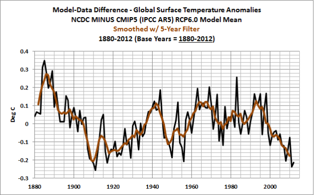
Figure 2
#######

Figure 3
COMPARISONS OF THE DIFFERENCE WITH GISS LOTI, HADCRUT4 AND NCDC DATASETS
The model-data differences for the 3 datasets are shown in Figure 4, using global latitudes, 90S-90N. All data have been smoothed with 5-year running-average filters. It should come as no surprise that the GISS- and NCDC-based curves are so similar—they use the same sea surface temperature dataset, NOAA’s ERSST.v3b. On the other hand, the HADCRUT4 data use the recently updated HADSST3 dataset. There’s another reason for the differences between the HADCRUT4 curve and the others: missing data is not infilled in HADCRUT4, while it is infilled in the GISS and NCDC products.

Figure 4
One of the big differences between the datasets are how they handle the polar data. GISS infills Arctic temperatures by masking sea surface temperature data anywhere there has been seasonal sea ice and by extending land surface temperature data out over the Arctic Ocean. GISS uses the same tactic in the Southern Ocean surrounding Antarctica. On the other hand, HADCRUT4 and NCDC products do not mask sea surface temperatures and extend the land surface temperature data out over the oceans. GISS also includes more land surface air temperature data in Antarctica than the other two datasets. And there are differences between the ERSST.v3b data used by GISS and NCDC and the HADSST3 data used in HADCRUT4. There is very little observations-based sea surface temperature source data in the Southern Ocean surrounding Antarctica. The missing sea surface temperature data is infilled in the ERSST.v3b data, but with HADSST3 it is not.
The easiest way to account for all of those differences is to exclude the data north of 60N and south of 60S. See the comparison in Figure 5. The GISS and NCDC curves are now almost identical, while the HADCRUT4 model-data difference continues to diverge from the others. The models, as shown in Figure 5, perform a little better during recent years if the polar data is excluded—but not much better.

Figure 5
OLD AND NEW GISS LOTI DATA
GISS recently switched to ERSST.v3b sea surface temperature data from a combination of the Hadley Centre’s infilled sea surface temperature data (HADISST) for the period of 1880 to 1981 and the satellite-based Reynolds OI.v2 data from 1982 to present. I haven’t yet found an explanation by GISS for that switch, but the obvious differences are presented in the post A Look at the New (And Improved?) GISS Land-Ocean Temperature Index Data. The model-data differences using the old and new GISS LOTI data are shown in Figure 6. The models actually performed better against the old GISS data before the 1920s. But there’s less of a difference between the models and the new GISS data from 1982 to present, meaning the new GISS data runs a little warmer over the past 30 years without the satellite-based sea surface temperature data. That’s to be expected. The satellite-based data Reynolds OI.v2 sea surface temperature data have better coverage, especially in the high latitudes of the Southern Hemisphere and much less infilling as a result.
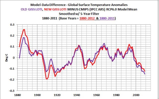
Figure 6
CLOSING
Presenting the differences between modeled and observed global surface temperatures is yet another way to show how poorly the climate models simulate global temperatures since 1880. The models cannot explain the observed cooling from 1880 to the 1910s, and they cannot explain the warming from the 1910s to the 1940s. Plotting the difference also helps to show that the divergence in recent decades, with the models simulating too much warming, started as far back as the early 1990s, when models overestimated the cooling from the volcanic aerosols associated with the eruption of Mount Pinatubo.
SOURCE
The GISS LOTI data and the outputs of the CMIP5-archived models are available through the KNMI Climate Explorer.
Its a shocking divergence of models from reality. Good work Bob.
Nice work Bob. Thanks for including Hadcrut data.
Good read. But, really, there are some people who still believe the official graphs of average global land and sea temperatures (NOAA) dating back to 1880 are actual observations.
The divergence between the models and
observationsadjusted temperauttues is roughly 1/2 of total warming. The other half is due to natural causes.Considering that the US has had no global warming in the past 100+ once you remove the adjustments, it should be no surprise that the models are diverging. They were trained using phoney data. In effect they are like Hal in 2001. They were given a lie and asked to make sense of it. Instead they went insane.
Interesting, thanks Bob.
From fig. 5 we have a range of differences between models and reality of approx .45C between 1885 and 1910 – that’s over just 25 years.
And we have approx 0.8C delta in observations between 1880 and 2012.
And we’re supposed to trust the models?
Climate models only go exponentially up. Reality since 1900 goes up and down every 30 years. All that AGW is solely based on 1975-2005 30-year natural warming trend, even milder than 1910-1945 one, and hockey-stick pseudoscience. CET and GISP2 record are enough to demolish the whole thing.
Thanks Bob.
I am confused Bob, if the plot is showing Model-data, should not the plot be positive after the year 2000 if the model has been higher than the actual temp data? Am I missing something?
Leo: Sorry about the confusion. The “-” in “Model-Data” in the title block is a hyphen. Most times, when people are discussing models and data place models first for some reason, so I stayed with that convention. On the second line of the title blocks, I clarify that the graph is of the Data MINUS the Model outputs.
Regards
Bob Tisdale:
I had to think about the post from Leo because the difference is the same whichever datum is subtracted.
But I think he has a point. Many people will think the graphs show the models are underestimating – not overestimating – warming.
Richard
I am a bit lost too. The conclusion reads “The models cannot explain the observed cooling from 1880 to the 1910s, and they cannot explain the warming from the 1910s to the 1940s.” If the observed data from the 1880 to the 1910s shows lower temps than the models, and the difference in the graph is positive, it would mean that you are subtracting the model output from the observed data. Same happens for the unexplained warming from the 1910s to the 1940s (where the difference is negative.)
That would also mean that after the late 1990’s the models are underestimating the observed warming. Don’t know where I got it wrong.
A point about forecast verification. In all meteorology verification that I know of and have done the convention is to do Forecast – Observed (Forecast minus Observed). It is the forecast that you are verifying against the real world observation. If the forecast is greater than the observed you will have a positive bias, and vice versa for a negative bias.
Thank you for the quick clarification Bob.
CFS says: “I am a bit lost too…”
Then I’ll provide you with a look at one of the original comparison graphs.
http://i34.tinypic.com/k37khs.jpg
Regards
Model minus observations: either natural processes not accounted for in the models, or the non-accounted for processes AND systemic adjustments either to the data or to generate better hindcasting?
If the latter is involved, then the disconnect between the models and the data are worse than it would appear.
We need to know what sort of hindcasting tweaking is NOT going forward.
Pamela Gray previously suggested that there are, indeed, two parts to the Scenario/History of temperature profiles, with a hindcast model different from the go-forward part. Is this true?
I agree with Leo. et al, about Model v. Actual. We are not examining how the Actual performed; that is assumed to be fact.
Instead we are interested in how the Model(s) performed. That is assumed to be the question. So I think the plot should be inverted. I do agree that the labeling is clear; so a readers should not have been confused for more than a moment.
To those who suggest that the graphs should be inverted: Either way that I presented them was going to be confusing, as differences often are. Here’s a sample graph of the difference with the data subtracted from the models:
http://i36.tinypic.com/vmyi43.jpg
I understand your arguments. However, the way I presented the difference in the post permitted me to write and for readers to see that the models were not able to explain the cooling from 1880 to the 1910s or the warming from the 1910s to the 1940s. In retrospect, I could have presented the graphs as you recommend, and then for the closing, I could have inverted the graph. For the next post about model-data differences, I’ll subtract the data from the model outputs. (It will be for sea surface temperature anomalies).
Regardless of how it’s presented, illustrating the difference is a great way to highlight the poor performance of the models.
Regards
Hind casting is used to tweak the first-draft models as a check of how their dials are interacting. However, there is a point where the modelers stop using historical data to tune their output (and different models do different types of tuning from historical temperature data).
To check the final version it is instructive to let the model run further back in time (I wonder how many bothered to do that). If their model is useless prior to their calibration period they had better not glue the dials in place till their model reproduces all historical records reasonably well. Once their model is set to their satisfaction, they let it run forward. It is no longer being tuned or tweaked by known observations.
Therefore the ONLY part of the model worth examining is the forward part and/or the backward part outside the tuning years calibration period.
Bob, I would suggest a tick mark that identifies the calibration period on your difference graphs, or just leave that middle part out altogether.
So a question for the scientists here: what would be an acceptable difference between any modeling tool and the actual measurements? Would .05 C, .10C , etc. across the timespan be an acceptable range to have confidence in any model? If we are arguing about +-.25C where the CO2 (a trace gas at only .04% of the atmosphere BTW) that would be noise compared to the 99.96% of the remainder of the atmosphere. Additionally, the mass of the ocean + land are orders-of-magnitude greater than all of the atmosphere.
Why not do something really simple: remove 100% of the CO2 factors from the models, then let those models predict past/future temperatures. Maybe those models could even account for land-use change factors as Dr. Roger Pielke Sr has suggested many times. Once those models are stabilized then add the small faction of CO2 back in and see what, if any, impact there is… maybe then also add in methane and other trace-gas factors, etc. one-by-one to see what, if any, impacts those small fractions impact the core results.
I have to laugh sometimes, if CO2 were the real “driver”, then Mars would be hotter than blue blazes. Just for grins… http://en.wikipedia.org/wiki/Atmosphere_of_Mars where CO2 = 95% of the atmospheric composition. OK, the total atmosphere is wispy but CO2 dominates…
Or maybe it’s about solar energy collection… or maybe other factors like strong planetary magnetic fields that drive ions/electrons into the atmosphere through the poles, maybe static-electric field differences throughout the atmosphere (a great electric insulator BTW), maybe very large surface area of H2O, etc… hmmm.
How about this for a postulate: 100% of the Earth’s atmosphere, therefore “climate”, is a response to the equilibrium of the mega-forces over very long periods of time.
Mental experiment: pretend 100% of the Earth atmospheric mass is wiped away (yep, temporary world-wide vacuum) then what will the atmosphere become given that all of the other current mega-forces continue? It might not be exactly the “same” as we have now, but some atmosphere will actually be rebuilt (ocean boils and freezes a little, some surviving plants, soil/water organisms, etc…), maybe with large portions of nitrogen, oxygen, argon, etc… until it resumes the approximate pressure and composition we now have.
Just sayin… we are myopically focused on an insignificant trace-gas effect and missing the bigger picture…
Pamela Gray –
Does the hind-casting tweak mean that the IPCC modelers have been rehindcasting every five years, so that there has not been, since 1993, any more than last five year, since-the-last-AR model to check for model-reality correlation?
As for the proxy use: tree rings and allenones are a constant record, unlike the 70-year or so ice core time smear. Certainly it is difficult to collect recent allenones as the most recent sediment is soft and liquid rich, (how about some imaginative data collection, like liquid nitrogen freezing of the top pond sediment, haul out a big frozen plug and sample back in the lab?) but tree-rings are not difficult to collect. Dendrochronologists have to have a constant, contiguous record to create their very accurate last 8000 years of records used to age-date wooden artifacts.
The data must be there to correlate the last 150 years of tree rings to instrumental data – even URBAN instrumental data.
Do we see it? Does Mann reference it? Or are modern temperatures special and non-relevant to pre-instrumental data times?
The following is HEAVY reading regarding model development (lots of maths), tuning, and what to do when a model is obviously bad (it just goes away). As far as I know, models are not tweaked once the modeler is satisfied with the calibration period. However new versions of the model may be considered, though I haven’t seen the usual sign of this happening (version number is usually attached to designate a new version of an old model). It may be useful to keep a new section on this site to archive model runs just in case tweaking happens without clear designation of that being a new version. I would think there might be a lot of incentive to produce a model that “somehow” gets it right. I would be alert. I can easily imagine a possible spliced model, mannian style, without an identifying label pointing out the splice. Thanks to Mikey for planting that seed. He is just so precious.
http://rsta.royalsocietypublishing.org/content/365/1857/2053.full
Plot each solar cycle peak back to 1910, adjust the scale factor, and see how it fits with those charts
I thought it would be helpful to plot a perfect model – data difference global anomaly comparison chart below. As you can see, a modellers goal is to be as close to 0 difference to the data as possible. 🙂
1
0 —————————————————————————————-
-1
Thanks Bob for the reply. That comparison graph explains where I got lost. Certainly interesting to see how the model expects more and more warming while the reality is that we have plateaued.