
Guest post submitted by Ken Gregory, Friends of Science.org
An analysis of NASA satellite data shows that water vapor, the most important greenhouse gas, has declined in the upper atmosphere causing a cooling effect that is 16 times greater than the warming effect from man-made greenhouse gas emissions during the period 1990 to 2001.
The world has spent over $ 1 trillion on climate change mitigation based on climate models that don’t work. They are notoriously poor at simulating the 20th century warming because they do not include natural causes of climate change – mainly due to the changing sun – and they grossly exaggerate the feedback effects of greenhouse gas emissions.
Most scientists agree that doubling the amount of carbon dioxide (CO2) in the atmosphere, which takes about 150 years, would theoretically warm the earth by one degree Celsius if there were no change in evaporation, the amount or distribution of water vapor and clouds. Climate models amplify the initial CO2 effect by a factor of three by assuming positive feedbacks from water vapor and clouds, for which there is little direct evidence. Most of the amplification by the climate models is due to an increase in upper atmosphere water vapor.
The Satellite Data
The NASA water vapor project (NVAP) uses multiple satellite sensors to create a standard climate dataset to measure long-term variability of global water vapor.
NASA recently released the Heritage NVAP data which gives water vapor measurement from 1988 to 2001 on a 1 degree by 1 degree grid, in three vertical layers.1 The NVAP-M project, which is not yet available, extends the analysis to 2009 and gives five vertical layers.
From the NVAP project page:
The NASA MEaSUREs program began in 2008 and has the goal of creating stable, community accepted Earth System Data Records (ESDRs) for a variety of geophysical time series. A reanalysis and extension of the NASA Water Vapor Project (NVAP), called NVAP-M is being performed as part of this program. When processing is complete, NVAP-M will span 1987-2010. Read about changes in the new version.
Water vapor content of an atmospheric layer is represented by the height in millimeters (mm) that would result from precipitating all the water vapor in a vertical column to liquid water. The near-surface layer is from the surface to where the atmospheric pressure is 700 millibar (mb), or about 3 km altitude. The middle layer is from 700 mb to 500 mb air pressure, or from 3 km to 6 km attitude. The upper layer is from 500 mb to 300 mb air pressure, or from 6 km to 10 km altitude.
The global annual average precipitable water vapor by atmospheric layer and by hemisphere from 1988 to 2001 is shown in Figure 1.
The graph is presented on a logarithmic scale so the vertical change of the curves approximately represents the forcing effect of the change. For a steady earth temperature, the amount of incoming solar energy absorbed by the climate system must be balanced by an equal amount of outgoing longwave radiation (OLR) at the top of the atmosphere. An increase of water vapor in the upper atmosphere would temporarily reduce the OLR, creating a forcing of more incoming than outgoing energy, which raises the temperature of the atmosphere until the balance is restored.

Figure 1. Precipitable water vapor by layer, global and by hemisphere.
The graph shows a significant percentage decline in upper and middle layer water vapor from 1995 to 2001. The near-surface layer shows a smaller percentage increase, but a larger absolute increase in water vapor than the other layers. The upper and middle layer water vapor decreases are greater in the Southern Hemisphere than in the Northern Hemisphere.
Table 1 below shows the precipitable water vapor for the three layers of the Heritage NVAP and the CO2 content for the years 1990 and 2001, and the change.
| Layer | L1 near-surface | L2 middle | L3 upper | Sum | CO2 |
| 1013-700 | 700-500 | 500-300 | |||
| mm | mm | mm | mm | ppmv | |
| 1990 | 18.99 | 4.6 | 1.49 | 25.08 | 354.16 |
| 2001 | 20.72 | 4.03 | 0.94 | 25.69 | 371.07 |
| change | 1.73 | -0.57 | -0.55 | 0.61 | 16.91 |
Table 1. Heritage NVAP 1990 and 2001 water vapour and CO2.
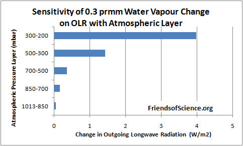
Dr. Ferenc Miskolczi performed computations using the HARTCODE line-by-line radiative code to determine the sensitivity of OLR to a 0.3 mm change in precipitable water vapor in each of 5 layers of the NVAP-M project. The program uses thousands of measured absorption lines and is capable of doing accurate radiative flux calculations. Figure 2 shows the effect on OLR of a change of 0.3 mm in each layer.
The results show that a water vapor change in the 500-300 mb layer has 29 times the effect on OLR than the same change in the 1013-850 mb near-surface layer. A water vapor change in the 300-200 mb layer has 81 times the effect on OLR than the same change in the 1013-850 mb near-surface layer.

Figure 2. Sensitivity of 0.3 mm precipitable water vapor change on outgoing longwave radiation by atmospheric layer.
Table 2 below shows the change in OLR per change in water vapor in each layer, and the change in OLR from 1990 to 2001 due to the change in precipitable water vapor (PWV).
| L1 | L2 | L3 | Sum | CO2 | ||
| OLR/PWV | W/m2/mm | -0.329 | -1.192 | -4.75 | ||
| OLR/CO2 | W/m2/ppmv | -0.0101 | ||||
| OLR change | W/m2 | -0.569 | 0.679 | 2.613 | 2.723 | -0.171 |
Table 2. Change of OLR by layer from water vapor and from CO2 from 1990 to 2001.
The calculations show that the cooling effect of the water vapor changes on OLR is 16 times greater than the warming effect of CO2 during this 11-year period. The cooling effect of the two upper layers is 5.8 times greater than the warming effect of the lowest layer.
These results highlight the fact that changes in the total water vapor column, from surface to the top of the atmosphere, is of little relevance to climate change because the sensitivity of OLR to water vapor changes in the upper atmosphere overwhelms changes in the lower atmosphere.
The precipitable water vapour by layer versus latitude by one degree bands for the year 1991 is shown in Figure 3. The North Pole is at the right side of the figure. The water vapor amount in the Arctic in the 500 to 300 mb layer goes to a minimum of 0.53 mm at 68.5 degrees North, then increases to 0.94 mm near the North Pole.

Figure 3. Precipitable water vapor by layer in 1991.
The NVAP-M project extends the analysis to 2009 and reprocesses the Heritage NVAP data. This layered data is not publicly available. The total precipitable water (TPW) data is shown in Figure 4, reproduced from the paper Vonder Haar et al (2012) here. There is no evidence of increasing water vapor to enhance the small warming effect from CO2.

Figure 4. Global month total precipitable water vapor NVAP-M.
The Radiosonde Data
Water vapor humidity data is measured by radiosonde (on weather balloons) and by satellites. The radiosonde humidity data is from the NOAA Earth System Research Laboratory here.
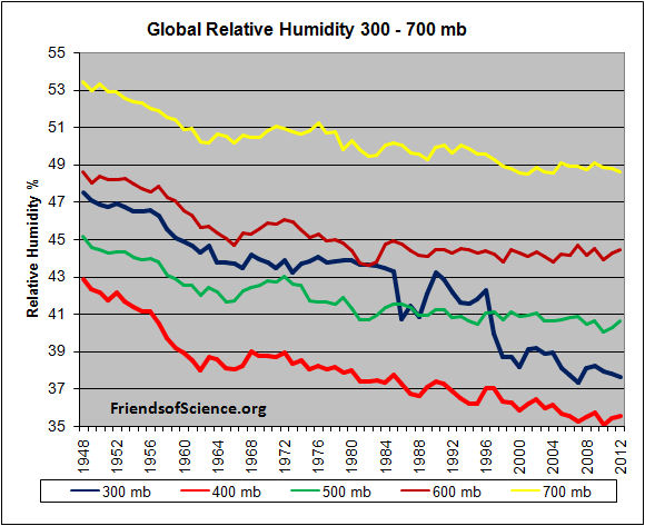
Figure 5. Global relative humidity, middle and upper atmosphere, from radiosonde data, NOAA Earth System Research Laboratory.
A graph of the global average annual relative humidity (RH) from 300 mb to 700 mb is shown in Figure 5. The specific humidity in g/kg of moist air at 400 mb (8 km) is shown in Figure 6. It shows that specific humidity has declined by 14% since 1948 using the best fit line.

Figure 6. Specific humidity at 400 mb pressure level
In contrast, climate models all show RH staying constant, implying that specific humidity is forecast to increase with warming. So climate models show positive feedback and rising specific humidity with warming in the upper troposphere, but the data shows falling specific humidity and negative feedback.
Many climate scientists dismiss the radiosonde data because of changing instrumentation and the declining humidity conflicts with the climate model simulations. However, the radiosonde instruments were calibrated and the data corrected for changes in response times. The data before 1960 should be regarded as unreliable due to poor global coverage and inferior instruments. The near surface radiosonde measurements from 1960 to date show no change in relative humidity which is consistent with theory. Both the satellite and radiosonde data shows declining upper atmosphere humidity, so there is no reason to dismiss the radiosonde data. The radiosonde data only measures humidity over land stations, so it is interesting to compare to the satellite measurements which have global coverage.
Comparison Between Radiosonde and Satellite Data
The specific humidity radiosonde data was converted to precipitable water vapor for comparison with the satellite data. Figure 7 compares the satellite data to the radiosonde data for the years 1988 to 2001.

Figure 7. Comparison between NOAA radiosonde and NVAP satellite derived precipitable water vapor.
The NOAA and NVAP data compares very well for the period 1988 to 1995. The NVAP satellite data shows less water vapor in the upper and middle layers than the NOAA data. In 2000 and 2001 the NVAP data shows more water vapor in the near-surface layer than the NOAA data. The vertical change on the logarithmic graph is roughly equal to the forcing effect of each layer, so the NVAP data shows water vapor has a greater cooling effect than the radiosonde data.
The Tropical Hot Spot
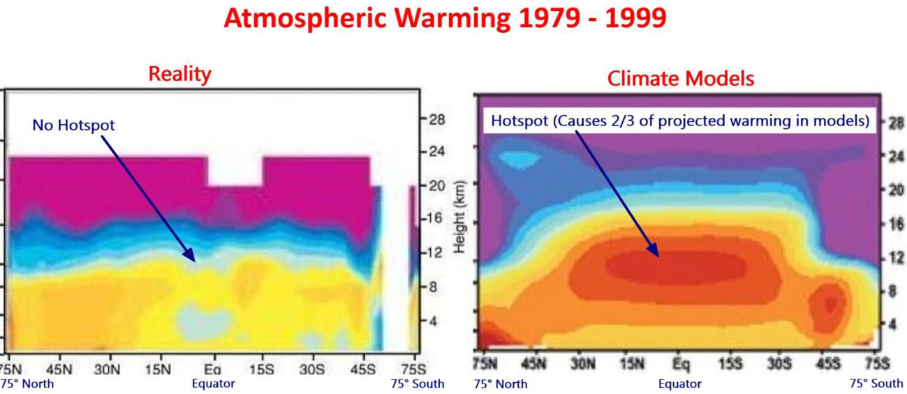
The models predict a distinctive pattern of warming – a “hot-spot” of enhanced warming in the upper atmosphere at 8 km to 13 km over the tropics, shown as the large red spot in Figure 8. The temperature at this “hot-spot” is projected to increase at a rate of two to three times faster than at the surface. However, the Hadley Centre’s real-world plot of radiosonde temperature observations from weather balloons shown below does not show the projected hot-spot at all. The predicted hot-spot is entirely absent from the observational record. If it was there it would have been easily detected.
The hot-spot is forecast in climate models due to the theory that the water vapor profile in the tropics is dominated by the moist adiabatic lapse rate, which requires that water vapor increases in the upper atmosphere with warming. The moist adiabatic lapse rate describes how the temperature of a parcel of water-saturated air changes as it move up in the atmosphere by convection such as within a thunder cloud. A graph here shows two lapse rate profiles with a larger temperature difference in the upper atmosphere than at the surface. The projected water vapor increase creates the hot-spot and is responsible for half to two-thirds of the surface warming in the IPCC climate models.

Figure 8. Climate models predict a hot spot of enhanced warming rate in the tropics, 8 km to 13 km altitude. Radiosonde data shows the hot spot does not exist. Red indicates the fastest warming rate. Source: http://joannenova.com.au
The projected upper atmosphere water vapor trends and temperature amplification at the hot-spot are intricately linked in the IPCC climate theory. The declining upper atmosphere humidity is consistent with the lack of a tropical hot spot, and both observations prove that the IPCC climate theory is wrong.
A recent technical paper Po-Chedley and Fu (2012) here compares the temperature trends of the lower and upper troposphere in the tropics from satellite data to the climate model projections from the period 1981 to 2008.2 The upper troposphere is the part of the atmosphere where the pressure ranges from 500 mb to 100 mb, or from about 6 km to 15 km. The paper reports that the warming trend during 1981 to 2008 in the upper troposphere simulated by climate models is 1.19 times the simulated warming trend of the lower atmosphere in the tropics. (Note this comparison is to the lower atmosphere, not the surface, and includes 10 years of no warming to 2008.) Using the most current version (5.5) of the satellite temperature data from the University of Alabama in Huntsville (UAH), the warming trend of the upper troposphere is only 0.973 of the lower troposphere in the tropics for the same period. This is different from that reported in the paper because the authors used an obsolete version (5.4) of the data. The satellite data shows not only a lack of a hot-spot, it shows a cold-spot just where a hot-spot was predicted.
Conclusion
Climate models predict upper atmosphere moistening which triples the greenhouse effect from man-made carbon dioxide emissions. The new satellite data from the NASA water vapor project shows declining upper atmosphere water vapor during the period 1988 to 2001. It is the best available data for water vapor because it has global coverage. Calculations by a line-by-line radiative code show that upper atmosphere water vapor changes at 500 mb to 300 mb have 29 times greater effect on OLR and temperatures than the same change near the surface. The cooling effect of the water vapor changes on OLR is 16 times greater than the warming effect of CO2 during the 1990 to 2001 period. Radiosonde data shows that upper atmosphere water vapor declines with warming. The IPCC dismisses the radiosonde data as the decline is inconsistent with theory. During the 1990 to 2001 period, upper atmosphere water vapor from satellite data declines more than that from radiosonde data, so there is no reason to dismiss the radiosonde data. Changes in water vapor are linked to temperature trends in the upper atmosphere. Both satellite data and radiosonde data confirm the absence of any tropical upper atmosphere temperature amplification, contrary to IPCC theory. Four independent data sets demonstrate that the IPCC theory is wrong. CO2 does not cause significant global warming.
Note 1. The NVAP data in Excel format is here.
Note 2. The lower troposphere data is: http://www.nsstc.uah.edu/public/msu/t2lt/uahncdc.lt
The upper troposphere data is calculated as 1.1 x middle troposphere – 0.1 x lower stratosphere; where middle troposphere is: http://www.nsstc.uah.edu/public/msu/t2/uahncdc.mt and the lower stratosphere is:http://www.nsstc.uah.edu/public/msu/t4/uahncdc.ls
============================================================
The original article is located at http://www.friendsofscience.org/index.php?id=483
Stick a fork in it. It’s done.
Of course instead of changing the computer models they will come up with yet another excuse for the lack of warming. The last thing they will do is admit they were in error.
Less Cloud = Colder????
Since when?
Do you have the data used to plot the global NVAP-M data in Fig. 4? I have been unable to get these data, which I need to superimpose over total column water vapor data measured almost daily in South-Central Texas from Feb 1990 to present. The NVAP-M data plotted in Fig. 4 and my plot show visual agreement and an overall slight decline that I would like to quantify. (I previously posted about NVAP-M at WUWT here: http://wattsupwiththat.com/2012/12/14/another-ipcc-ar5-reviewer-speaks-out-no-trend-in-global-water-vapor/)
“Most scientists agree that doubling the amount of carbon dioxide (CO2) in the atmosphere, which takes about 150 years, would theoretically warm the earth by one degree Celsius if there were no change in evaporation”
Why? are they really sure?
Figure 8 only shows data up to 1999. Is there a plot available with data since then?
Someone needs to ask Jim Hansen, publicly, with tape rolling, what he thinks of this report. Doesn’t it blow the entire AGW CO2 Based Climate Change theory right out of the water?
Will NASA science data be ignored by NASA “scientists” like Hansen?
Global cooling is on the way!
Why does the upper atmosphere satellite data humidity decline after 1995 more than the radiosonde humidity data? Is there some reason upper atmosphere humidity would decline more over the oceans than over land?
The IPCC dismisses the radiosonde data as the decline is inconsistent with theory.
Pretty much says it all. Just like the Mann trick as described by Dr. Susan Crockford today:
http://polarbearscience.com/
CAGW ! ? or what ever they are calling the “religion” today. It makes ya wanna weep.
More evidence of global cooling. There will be no lack of ice for my Mai Tai. 🙂
Prost!
Time to take the AGW theory out of the oven – it’s done.
Check you dates in your conclusion. Is it 1998 or 1990?
Either way, this is another huge hurdle for “the CAGW cause!”
oops wrong anecdotal citation (and one more);
20 meters of snowfall in Hokkaido;
Climate warming boogieman blamed, oh my…
I’m waiting for the first one to publish a paper plotting atmospheric CO2 vs upper atmospheric water vapor.
“The NVAP-M project, which is not yet available, extends the analysis to 2009 and gives five vertical layers.”
Although not available yet, it is already understood: the data beyond 2001 has, in somebody’s computer, been added to the program that produced the earlier profiles. It is only the desire to have greater detail and certainty of results that has stopped the new data from being released.
If the new data contradicted the older data, that would have been put in a press release to discredit the initial speculations that everyone knows was going to happen. The silence tells you that the new data is not supportive of CAGW.
People like Hansen and Gore already know about stuff like this. It is in their career, persona and financial interests to be aware of whatever is happening that might aid or detract from their positions.
How Stoat/Connelly/Tamino will spin this, I’ll be interested to see. Perhaps they will say it is because of aerosols. Or volcanoes. Probably just say it is not important.
Maybe some of that water vapor is in the oceans or maybe here:
http://www.abqjournal.com/main/2013/02/26/abqnewsseeker/some-roads-still-closed-in-panhandle.html
But, but, but the decline in water vapour is down to global warming! Don’t you, erm, get it?
Well, it’s just like I always thought, the IPCC’s theories don’t hold water!
Maybe this is a negative feedback. Maybe this is due to a cooler sun. But because alarmists claim that water vapor is a high-sensitivity amplifier of carbon dioxide warming will have a problem with this situation.
Alarmists who try to claim that water vapor has decreased because of their much-claimed high sensitivity to carbon dioxide will also have to admit that the water vapor has decreased due to cooler temperatures, because carbon dioxide’s higher temperatures are supposed to force more water vapor.
Now I’m truly confuzzed. I was told that globull warming would cause more frequent and serverer storms because of more evaporation,thus more water to come back home.Now there is less atmospheric water vapour,so less warming,so wouldn’t the converse of less storms and less precipatation be true? My head hurts,and it’s to darn early for a drink!
“Four independent data sets demonstrate that the IPCC theory is wrong. CO2 does not cause significant global warming.”
I suggest that this final statement of your conclusion should be qualified just a bit. How about “the supposed forcing from water vapor does not magnify the forcing from CO2 alone.”
Correction needed in the conclusion. Data goes from 1988 to 2001 not 1998 to 2001.
I forgot to say that I enjoyed your essay. Good work.
Sorry, where is the “decline”?
The data (Fig. 1) show a significant INCREASE in total water wapor after 1997, just as expected.
Warmer temperatures near surface (as expected) -> more water vapor.
Lower temperatures in the higher layers (as it should be) -> less water vapor.
What counts is the total water vapor in the column and this is decided by the lower levels of the atmosphere, where most of the moisture is concentrated.
Perfect agreement with the CAGW theory.
Sorry, your analysis must be more careful.
Alex – this is not true. Yes the total water vapor may well increase but what really matters is the concentration in the upper atmosphere which defines the effective emission height. This determines how much radiation escapes to space. Everything below that is more or less determined by thermodynamics (convection evaporation and the lapse rate). The height of the troposphere depends on CO2 AND H2O. This then determines the surface temperature because convection stabilizes the lapse rate.
Umm … fair enough. But how come it did not cool between 1990 and 2001?
Great work! a Climate Detective at large.
Thank you, Ken Gregory!
WOW! This strikes right to the heart of falsifying the hypothesis that man made CO2 is the primary cause of ‘global warming’. I’ll read this again in detail later today, as my lunch break time is limited but….this is good analyses!
MTK
OK, so this lack of water vapour is our fault, our grandchildren will all die of thirst – what should we tax next?
These results back up the previous WUWT posts namely:
New paper on Global Water Vapor puts climate modelers in a bind
and
Another IPCC AR5 reviewer speaks out: no trend in global water vapor
Radiative transfer through the atmosphere is mostly controlled by water vapour, because its concentration is changing rapidly whereas CO2 is essentially constant. As a result radiative cooling of the surface increases rapidly for dry atmospheres, which then reduces the convective losses. In deserts radiation loss dominates heat transfer whereas convection dominates heat transfer in the tropics. At night deserts cool quickly through radiation whereas the tropics remain warm at night when convection halts. Therefore it is H2O that controls the balance between radiative cooling and convective/evaporative cooling of the surface.
The CO2 radiative transfer for fixed concentration is not actually constant but depends also on humidity levels in the upper atmosphere because some H2O absorption lines overlap with the CO2 lines. The effective emission height for H20 outside the 15micron band is in general lower than for CO2 because most humidity is concentrated in the lower levels of the atmosphere. However what matters for CO2 feedback is the water vapour content at the top of the troposphere. If H20 levels fall in this region then this can completely offset any increases in CO2. So in terms of radiative forcing at the TOA.
RF = 5.2 Ln(C/C0) – X Ln(H/H0)
Ken’s work shows that the NVAP-M data support ‘X’ acting as a negative feedback.
Haven’t fully absorbed it all, but this has the potential of being quite a big deal
obviously your hygrometer needs to be adjusted………/snark
WOW!!!!! If only there would notice of this in the main [stream] news outlets.
Before we pop a cork and have parades and things, we should wait for the updated data. 2001 was quite a while ago.
I’m struggling with the statement (critical to the conclusions) that the change on OLR (as a ratio to change in water vapor) for upper layers is orders of magnitude more than for lower layers. Can someone provide a physical explanation why this is plausible? I realize that someone has measure this, they aren’t simply hypothesizing it, but I’d like to know why it is so.
another decline? quick – hide it!
Richard says:
March 6, 2013 at 11:15 am
‘“Most scientists agree that doubling the amount of carbon dioxide (CO2) in the atmosphere, which takes about 150 years, would theoretically warm the earth by one degree Celsius if there were no change in evaporation”
Why? are they really sure?’
Some say that the figure is Arrhenius’ estimate from laboratory work. Some say that it is Richard Lindzen’s best guess. If the latter is true, I think he was just throwing a bone to the mainstream. There might be other “sources.”
No one has a clue what the value is in the atmosphere. That is because forcings and feedbacks are at work in the atmosphere and the magnitudes of the forcings and feedbacks are unknown.
A C Osborn says:
March 6, 2013 at 11:11 am
The article doesn’t mention clouds. Clouds contain liquid water. We are talking about water vapor.
Forrest M. Mims III says:
March 6, 2013 at 11:13 am
The NVAP-M data has not been released. Mary Jane Saddington of the NASA Langley ASDC User Services wrote in January, “First, please be aware that a new dataset, in netCDF
format will be available in the March timeframe.” Its not there yet. However, the Vonder Haar et al (2012) paper (see the link under Figure 3) shows on page 16 the annual global total precipitable water vapor (not by layer) of every second year from 1988 to 2008.
Richard says:
March 6, 2013 at 11:15 am
The 150 years is the actual CO2 increase from 1960 to 2012 plus 0.5%/year thereafter.
Most scientists that have carefully considered the no-feedback case would agree that a CO2 doubling would cause about a 1 C increase in temperature, but recognized that this theoretical result could never happen. A warming must cause a change in evaporation, which is a strong negative feedback.
Ian H says:
March 6, 2013 at 11:51 am
Good catch! I’ll correct it on my website.
Maybe Patchy should get back to running steam engines and get some
water vapor back into the atmosphere…
No surprise here. The colder it gets the more moisture gets frozen out of the atmosphere!
Checking the links in the above shows there was a paper published online on Aug 3 in GRL:
Thomas H. Vonder Haar1,2,*, Janice L. Bytheway1,2, John M. Forsythe1,3
Article first published online: 3 AUG 2012
DOI: 10.1029/2012GL052094
Can anyone get the full pdf (behind a paywall)?
The abstract was uninformative:
“Keywords: climate data record;water cycle;water vapor
[1] The NASA Water Vapor Project (NVAP) dataset is a global (land and ocean) water vapor dataset created by merging multiple sources of atmospheric water vapor to form a global data base of total and layered precipitable water vapor. Under the NASA Making Earth Science Data Records for Research Environments (MEaSUREs) program, NVAP is being reprocessed and extended, increasing its 14-year coverage to include 22 years of data. The NVAP-MEaSUREs (NVAP-M) dataset is geared towards varied user needs, and biases in the original dataset caused by algorithm and input changes were removed. This is accomplished by relying on peer reviewed algorithms and producing the data in multiple “streams” to create products geared towards studies of both climate and weather. We briefly discuss the need for reprocessing and extension, steps taken to improve the product, and provide some early science results highlighting the improvements and potential scientific uses of NVAP-M.”
And the slow descent in to the next ice age continues despite Man[n]
they will be hung by their own comments IE} more heat means more water vapour!
Given models and the analysis of real data, I’ll go with the data everytime. How long till the popular media and the public wake up to being hoodwinked by the CAGW bureaucratic boondoogle?
More importantly, a reduction in water vapor content of the atmosphere lowers its enthalpy. The lower humidity alone could account for all the atmospheric temperature increases as less heat is required to raise the ‘temperature’ of the drier atmosphere.
Yep. CO2 merely changes the height at which radiative balance takes place. Water vapor adjusts to maintain equilibrium. Instantly. CO2 drives changes in water vapor such that radiative balance is maintained. The cooling / vapor transport mechanisms of the lower layers don’t change with CO2 so the balance is maintained by reducing GHG’s (water vapor) in the upper atmosphere.
It’s worse than we thought. Maybe the temperature won’t change at all, but we’ve gone and upset the balance of the water vapor.
Airplanes will fly better. The horror!
The whole idea that H20 is not a forcing, it’s a feedback is the source of the error from the beginning. The notion that the “Team” still holds onto its golden goose in the light of more than a decade of contradictory real world evidence just shows how entrenched the players in this money pit are. The enhanced greenhouse theory has been dead for years now, yet we still have people hanging on for dear life. It’s inexplicable from a scientific viewpoint. Positive feedback doesn’t even make intuitive sense.
Josh could come up with a good cartoon for that one I’m sure (showing LWR interacting with 1 CO2 molecule and 1 H2O. Each one carries a sign… Josh take it from there)
We have moved into a world of science where (as long as it’s climate) observations don’t matter. Whether it’s water vapour decline, AWOL hotspot or flat temps for over 15 years, none of it really matters to the faithful. The theory and models must be defended no matter how many times they are falsified.
The world has spent over $ 1 trillion on climate change mitigation based on climate models that don’t work. They are notoriously poor at simulating the 20th century warming because they do not include natural causes of climate change – mainly due to the changing sun – and they grossly exaggerate the feedback effects of greenhouse gas emissions.My bold.
It is the understanding of natural oscillations of both sun and the Earth combined, which opens possibility of the implementation in the climate change science.
http://www.vukcevic.talktalk.net/EarthNV.htm
I think the graphs are visually misleading … note the log scale! So the visual decline at the top of the atmosphere *looks* like it is hugely greater than the increase near the surface, but its not!
To draw valid conclusions we need to see the changes compared in absolute terms.
“I think the graphs are visually misleading … note the log scale! ”
Log scales make sense because we are addressing TOA radiative forcing.
Wow!
Dynamite!
@highflight56433 says: Maybe some of that water vapor is in the oceans
Yeah, the missing water vapor has been found.. in the deep ocean!
alex says:
March 6, 2013 at 11:56 am
Sorry, where is the “decline”?
——————-
The near surface increse has next to no effect upon OLR. The lower part of that chart showns the least moisture, ie, at high alltitudes. where the effect on OLR is extreme. That is where the decline is. in other words, a very big cooling effect of the decline in humidity. Does any of it relate to CO2? Who knows!(the science is settled is it not?/sarc off)
Myron Mesecke at 11:11 am. The IPCC may look for more overwhelming evidence, hoping that this overwhelms the falsifications. Go to the beach and you will get overwhelming evidence that the earth is flat, and ask Al Gore to twitter this over the internet. From the pre-post-modern Age we still have a logical asymmetry. A false theory may have both true and false consequences. A true theory only has true consequences. Therefore, if a theory makes false predictions, it must be false, whereas nothing follows from overwhelming evidence. Also late Karl Popper would have said ‘stick a fork in it. It’s done’ and the IPCC can be disbanded.
Alex, you must have missed the section below. It explains why a slight increase at near-ground levels is not as important as the decreases at higher levels.
Sara Hindle says:
March 6, 2013 at 11:33 am
The upper atmosphere (500 to 300 mbar level) water vapor is quite variable over space and time, as shown in this animation I made:
http://www.friendsofscience.org/assets/documents/FOS%20Essay/NVap300-500mb1988-99.gif
from:
http://www.friendsofscience.org/assets/documents/FOS%20Essay/Climate_Change_Science.html#Water_vapour
The study of decline water vapor in the Stratosphere by Solomon et al (January 2010) blames the water vapor decline on El Nino. The paper says,
So I expect that ocean process are also responsible for more water vapor decline in the upper troposphere over oceans than over land.
Of course, part of the decline could be due to instrumentation and calibration problems, but this is currently the best data available. Our theories and policy decisions should be based on the best available data.
Ole Humlum’s site, http://www.climate4you.com/ , has lots of data on water vapor in the upper atmosphere. Go to his Climate and Clouds section. Water vapor and relative humidity have been declining for many, many years.
shows declining upper atmosphere water vapor during the period 1998 to 2001
======
doesn’t fit CO2 (opposite), doesn’t fit sun spots, doesn’t fit temps, ENSO, nada etc
…can anyone think of a biological fit? plants? bacteria?
What would make water vapor levels steadily fall…..as CO2 levels steadily increase?
“IPCC dismisses the radiosonde data as the decline is inconsistent with theory.” I take sound empirical data over numeric models that are known to be inaccurate any day. That is how science is supposed to be done, not by crystal ball and faith.
Justthinkin says:
March 6, 2013 at 11:50 am
No, table 1 shows there was an increase of total water vapor between 1990 to 2001 of 0.61 mm. But there is less upper atmosphere water vapor (700 to 30 mb) which has a 5.8 times greater effect on OLR, and surface temperatures, than the increased water vapor in the lower atmosphere (1013 to 700 mb).
The amount of upper atmosphere water vapor has little to do with the precipitation and evaporation rates.
Cold periods always have more severe weather. The theory of CO2-induced warming would increase temperatures in polar regions more than temperate or tropical regions, so reducing the temperature differences that powers storms. The storm Sandy was made large by a very cold front colliding with a tropical storm.
You might want to read NASA’s statement on using NVAP for multidecadal trends:
http://nvap.stcnet.com/NVAP_Trend_Statement.pdf
Quick summary: don’t do it!
Is there an easy way to spatially overlay the CO2 distribution data with this water vapor content?
“Many climate scientists dismiss the radiosonde data because of changing instrumentation and the declining humidity conflicts with the climate model simulations. ”
An inconvenient truth, so to speak?
Richard says:
March 6, 2013 at 11:15 am
“Most scientists agree that doubling the amount of carbon dioxide (CO2) in the atmosphere, which takes about 150 years, would theoretically warm the earth by one degree Celsius if there were no change in evaporation”
Why? are they really sure?
===========
Are they sure? Of course they’re sure. Do they have the slightest idea what they are talking about? Not necessarily. 1.6 degrees per doubling is what Svante Arrhenius predicted back in 1906 or so (after scaling back his initial, larger, estimates) and the CO2 increase rate is measured by the measurement program set up by Charles Keeling in the 1950s. If there is any science at all in climate science Arrhenius and Keeling are surely part of it.
weather postpones climate:
6 March: Washington Times: Stephen Dinan: Hill hearing on global warming cancelled by D.C. snowstorm
An unusually chilly March day and the snowstorm it spawned have shut down much of official Washington on Wednesday — including a hearing House Republicans had called to examine global warming.
“Postponed due to weather,” read the notice from the House Science, Space and Technology Committee sent in the morning.
The hearing was scheduled to give House lawmakers a comprehensive briefing on how well scientists understand the climate and humans’ effects on it as a means “to inform decision-making on potential mitigation options.”…
http://www.washingtontimes.com/blog/inside-politics/2013/mar/6/hill-hearing-global-warming-cancelled-dc-snowstorm/
My ebook, The Arts of Truth, made the same observations last year using data other than NVAP (since not enough NVAP years were publicly available). What is more interesting is how IPCC AR4 chose to dismiss or ignore all of the contrary evidence that existed then, strengthened since by what we know now. Extreme selection and confirmation bias. Yet it continues in the leaked AR5 SOD. Proof not just of uncertain science, but of deliberately bad science. Mannian, one might say.
This should comprehensively disprove the Global Warming theory.
But nobody will ask the critical question. So it will not disprove the theory.
I suggest that readers here send a letter/email to their local political representatives – Congressmen or Senators in the US, MPs in the UK, and so on, describing how the theory critically depends on increased water vapour, how research is showing that water vapour is not increasing, and asking why this does not disprove the hypothesis. If enough politicians ask the relevant government scientists questions like this something is going to have to give…
Alex,
According to the IPCC draft there is “no trend” in the total column in spite of (at least until very recently) increasing average ocean surface temperature and enthalpy.
Myron: http://wattsupwiththat.com/2013/03/06/nasa-satellite-data-shows-a-decline-in-water-vapor/#comment-1240820
The last thing that they will never admit is that man did not cause it . . . .
Translated, it IS still man made . . . . humans CAN/DO control the changes (variations).
Logically, climate models say that precipitation should also have increased over that period, but satellite- and rain guage-based precipitation data shows that global preciptation has decreased:
http://bobtisdale.wordpress.com/2012/12/27/model-data-precipitation-comparison-cmip5-ipcc-ar5-model-simulations-versus-satellite-era-observations/
Wow. A killer blow, it is.
Moreover, water vapor is not a well mixed gas, its distribution is fractal-like. It means average water vapor concentration in a layer / grid box only puts a lower bound on transparency of that volume in IR bands dominated by water vapor absorptivity / emissivity. That is, it can be arbitrarily transparent if distribution is sufficiently uneven (a wire fence is much more transparent than a thin metal plate, even if it contains the same amount of material per unit area).
Scale invariant features of distribution (e.g. fractal dimension) are not well represented in a gridded database.
The reason water vapor distribution is a fractal is that water vapor content of each parcel is determined by its history, that is, by its temperature the last time it got saturated. This event might have occurred several days or weeks ago. In the meantime turbulent flows distorted that, originally bulky parcel into a mesh of thin threads, interwoven by other parcels of a completely different history. That’s how water vapor distribution looks like at any specific moment and this is why shape of clouds is always fractal-like, for the “surface” of a cloud is nothing else but the surface separating a region of saturation from others with lower relative humidity. Geometry of each constant relative humidity surface is like that, even if most of them are invisible to the naked eye.
Trying not to be a conspiracy nut, but since NASA is a government funded organization, and US taxpayers fund it i.e. – We paid for this information. Why and who has been sitting on this information for the entire “Global Warming” time period. The data start in 1988 and from the shown graph by 1995 the “causes more water” theory was shot down.
Talk about hide the decline.
Reblogged this on UNCOVER777.
@ Dodgy Geezer:
One would think that this would signal the beginning of the end for the AGW hypothesis. The problem, though, is not one of proving or disproving the science. Progressive Green – environmentalism – is an ideology bordering on a religion. They will not give up their beliefs and their collectivist objectives so easily.
alex says:
March 6, 2013 at 11:56 am
The main point of the post is to dispel this myth. The total water vapor column amount is of little relevance to the forcing and global warming. A small water vapor change in the upper atmosphere has a large effect on OLR. Have a look at Figure 2.
Cees de Valk says:
March 6, 2013 at 11:58 am
Temperatures have risen from 1975 to 2002 because the sun reached a maximum magnetic flux activity in 1990, causing a maximum temperature response in about 2002.
http://www.friendsofscience.org/assets/documents/FOS%20Essay/Rao_CR_HMF.jpg
In 1990, the sun was more active than at any time in the past 8000 years.
http://www.friendsofscience.org/assets/documents/FOS%20Essay/SolarActivity8000Years.gif
The sun’s magnetic flux affects the cosmic ray flux to earth, which changes cloud cover. It also has an effect on upper atmosphere electric currents, and ozone levels which affects climate.
The upper atmosphere water vapor change was a negative feedback to the warming effects of both CO2 and the sun-induced warming.
The Other Phil says:
March 6, 2013 at 12:17 pm
See Clive Best’s comment March 6, 2013 at 12:01 pm.
Generally, outside of the atmospheric window, a photon of radiation emitted by the lower atmosphere can travel only a short distance before being absorbed by water vapor. Most of the heat energy from the lower atmosphere must move up by convection to an altitude high enough in the atmosphere where the water vapor concentration is low enough that it can escape to space without being absorbed by a greenhouse gas molecule. All this is calculated by line-by-line radiative code computer programs that use thousands of measured absorption lines from the HITRAN data base.
O/T but RSS confirm the sharp fall in temps that UAH did in Feb.
Temps are back to Nov/Dec levels, i.e by historical levels, pretty low.
http://notalotofpeopleknowthat.wordpress.com/2013/03/06/satellite-temperatures-latest/
Theo Goodwin says:
March 6, 2013 at 12:22 pm
You don’t need to know the value of feedbacks to calculate the no-feeback climate sensitivity. The no-feedback climate sensitivity to double CO2 is calculated by climate models where water vapor, clouds, ice, evaporation etc. are held constant. It is about 1 C.
The bottom line for separating science from nonsense is the recognition of massive model error or insignificant terms comprising the model. It is political science when the model errors don’t matter and the message continues on unabated.
Lance Wallace says:
March 6, 2013 at 12:39 pm
I provided a link to the Vonder Haar et al (2012) paper just above Figure 4.
What has been happening since 2001 ?
I would expect to see a cessation of the decline or a slight recovery
Some have argued for atmospheric heat energy to be used as a better and more meaningful metric than a supposed global mean temperature. Heat is a product of temp and water content. Viewed this way, decreasing water vapour could mean that increasing temperatures have not reflected increasing heat.
Rattus Norvegicus says:
March 6, 2013 at 1:28 pm
You are joking, right?!
The NVAP-M people released just the irrelevant total water vapor column even-year annual numbers only, but not the by-layered data. We don’t want to confuse the IPCC lead authors preparing the AR5 with inconvenient data!/sarc
Janice L. Bytheway, co-author of the Vonder Haar (2012) paper and NVAP-M team member wrote in an email to me 7/24/2012:
“As for your interest in the trends at the upper versus lower levels of the atmosphere, we unfortunately don’t have the staff or funding to provide subsets of the data at this time.”
A strange response since the total column amount is just the sum of the layers.
Again, this is the best available data. We expect that the data might improve, or be adjusted in the future, for better or worst. Of course we should use it, even if the result is embarrassing to the NASA team. They will get abuse from their climate alarmist colleagues, but we can hope it will not be as severe as what Phil Jones feared from his pals when he admitted there was a pause in global warming. Phil said “They will kill me!”
As the temperature standstill continues and evidence continues to trickle in that CAGW theory is failed, there is a sense of panic at the global warming centres of excellence dotted around the world. Pachauri will soon head off to greener pastures as he ralises the jig is up. Gore left the field some time last year (sold TV to oil, dumped green investments). As the scam unravels you will witness increased infighting as the rats bolt for the exits which are flooding with water.
Spanner in the works…but will not be discussed in the msm
At least one part of this story is completely wrong. The “friends of Science” link to the paper of Vonder Haar et al. (2012), the text of which is unfortunately behind a pay-wall. The article states:
The strength of the NVAP-M dataset is its global overview of humidity. Because the number and types of the satellites change during the period studied and because the orbit of the satellites change during their life time, the dataset is not homogenenous. They did work on improving the homogeneity of the data, but this work is not finished. Its trends should not be interpreted.
This should have been known with Anthony Watts. Forest Mims above links to his guest post about the NVAP-M dataset. Already here I have explained in the comments that the authors of the NVAP-M dataset do not think their data can be used for trend analysis.
“Trying not to be a conspiracy nut, but since NASA is a government funded organization, and US taxpayers fund it i.e. – We paid for this information. Why and who has been sitting on this information for the entire “Global Warming” time period. The data start in 1988 and from the shown graph by 1995 the “causes more water” theory was shot down.
Talk about hide the decline.”
Hear, hear! NASA is sitting on this as it will end Hansen, expose a lot of nonsense in a lot of models, and rearrange a lot of people’s careers. Wonder if Obomination has anything to do with it? He does have his fingers in a lot of pies. FOIA, anyone? Ken Gregory, you know where the bodies are buried?
That’s weird my other post got lost.
“Maybe the water vapour is not making it to the upper layer.”, i postulated; then i cited a few youtube posts about “record snowfall 2013”, and “russia snowfall 2013″…one example from North America, Russia, and Japan. But i accidentally used the wrong URL for the Japan example, instead i referenced to a record breaking snowball fight in Utah (this was a cool clip).
Ken Gregory says:
March 6, 2013 at 2:39 pm
“….You don’t need to know the value of feedbacks to calculate the no-feeback climate sensitivity. The no-feedback climate sensitivity to double CO2 is calculated by climate models where water vapor, clouds, ice, evaporation etc. are held constant. It is about 1 C.”
/////////////////////////////////////////////////////////////////////////////////
But we live in the real world, and what is relevant to the real world is the effect of feedbacks on that ‘theoretical’ figure. If these feedbacks are negative then less than 1C will enure, and if positive then more that 1C will enure.
If one looks at the satellite data (33 years) if one removes the 1998 super El Nino (which no-one suggests was caused by CO2) then first order correlation with CO2 emissions over those 33 years is essentially zero (flat between 1979 and 1997 and flat between 1998 to 2012). This data therefore supports the view that feedbacks may well be negative.
Moderators CORRECTION, plse
Ken Gregory says:
March 6, 2013 at 2:39 pm
“….You don’t need to know the value of feedbacks to calculate the no-feeback climate sensitivity. The no-feedback climate sensitivity to double CO2 is calculated by climate models where water vapor, clouds, ice, evaporation etc. are held constant. It is about 1 C.”
/////////////////////////////////////////////////////////////////////////////////
But we live in the real world, and what is relevant to the real world is the effect of feedbacks on that ‘theoretical’ figure. If these feedbacks are negative then less than 1C will enure, and if positive then more that 1C will enure.
If one looks at the satellite data (33 years) if one removes the 1998 super El Nino (which no-one suggests was caused by CO2) then first order correlation with CO2 emissions over those 33 years is essentially zero (flat between 1979 and 1997 and flat between 1999 to 2012). This data therefore supports the view that feedbacks may well be negative.
phlogiston says:
March 6, 2013 at 3:09 pm
Ya, it could be called Earth Enthalpy (EE). Then the anomaly in enthalpy could be referred to as exo or endo…i love it!!! EEE or EEE*
That would be a great metric for Global Whatever!
Berényi Péter says:
March 6, 2013 at 1:53 pm
The reason water vapor distribution is a fractal is that water vapor content of each parcel is determined by its history, that is, by its temperature the last time it got saturated. This event might have occurred several days or weeks ago. In the meantime turbulent flows distorted that, originally bulky parcel into a mesh of thin threads, interwoven by other parcels of a completely different history. That’s how water vapor distribution looks like at any specific moment and this is why shape of clouds is always fractal-like, for the “surface” of a cloud is nothing else but the surface separating a region of saturation from others with lower relative humidity. Geometry of each constant relative humidity surface is like that, even if most of them are invisible to the naked eye.
Bold emphasis is mine. This is an interesting concept… one I had not considered before. Thank you for this insight BP!
MtK
DD More says:
March 6, 2013 at 1:55 pm
>>>>>>>>>>>>>>>>>>>>>>>>>>>
Keep trying!
Scientific information has become proprietary.
Enough Americans have been objecting to this lately the gov agreed to allow limited access (12 months) on some scientific research, but they haven’t followed through on this (that im aware). We will see (hopefully) if there is granted access or that a surprising amount of science is really classified…at least then we would know hahaha
Viz: Laurie Bowen post:
http://wattsupwiththat.com/2013/02/22/king-obama-to-circumvent-lawful-due-process-on-climate/#comment-1231260
In Canada, the scientists are leaking to the press that they have been muzzled as a condition of employment. Whistleblowers Preventative measures, excellent.
http://sciencewriters.ca/initiatives/muzzling_canadian_federal_scientists/
“An analysis of NASA satellite data shows that water vapor, the most important greenhouse gas, has declined in the upper atmosphere”
So I guess that next NASA will be telling us where that water has gone, and that the polar ice caps and glaciers are in fact growing…. Or are they going to tell us that this missing water is ALSO hiding at the bottom of the ocean….
It would be nice to see the 2001 data plotted on figure 3 with the 1991 data.
Thanks for the post.
Water vapor (and cloud) feedback is the make or break for this general theory.
These ARE the most important aspects to consider and measure regarding if there will be significant global warming from GHG increases or not. They really are.
So far, they appear to be around Zero (maybe slightly positive or maybe slightly negative).
If they do turn out to be Zero (or slightly positive or slightly negative), warming is nothing to worry about. This issue raised by Ken is the most important one there is regarding this theory.
One might have to do the math in terms of how the feedbacks multiply on top of each other to get us up to 3.0C per doubling and how small changes in these feedback on feedback values would leave completely different results but this point should not be under-estimated. If I was in the conspiracy camp, I might conclude the feedback impacts were carefully tuned to reach a 3.0C per doubling level rather than determined based on how the climate operates.
Don’t worry we’ll just have a nuclear winter to offset the global warming – will all balance out nicely …according to the models of course ….
[snip – I suggest you try again without the accusations Joel – Anthony]
Note the declining atmospheric water vapour over the last 20 years is also shown in Forrest M. Mims III’s work
http://www.forrestmims.org/sciencedata.html
Total Column Water Vapor (1990 to 2010)
Have you submitted this for publication?
Ken Gregory says:
March 6, 2013 at 1:26 pm
Justthinkin says:
March 6, 2013 at 11:50 am
Ken…thank you for the reply….I may be a bit old, but I was taught in aeronautical engneering,the lower the temp diff between the poles and the equator,the less severe the weather. The way my prof from the RCAF(which shows how old I am) put it…in layman’s terms….when a male and female are both hot to trot,less resistance,disturbance,and more friction (which is good),therefore less turbulance and storms. A bit crude,but to the point.And yes,I do know the diff between vapour and liquid..should have added the /sarc tag. Mea Culpa.
Meh. Probably will, except alarmists will claim that reduced water vapour is a sign of impending doom and desertification caused by a different more dangerous, worse than we thought type of co2.
“The world has spent over $ 1 trillion on climate change mitigation based on climate models that don’t work. They are notoriously poor at simulating the 20th century warming because they do not include natural causes of climate change – mainly due to the changing sun – and they grossly exaggerate the feedback effects of greenhouse gas emissions.”
You mean like these models?
http://www.ipcc.ch/publications_and_data/ar4/wg1/en/figure-9-5.html
http://web.archive.org/web/20100322194954/http://tamino.wordpress.com/2010/01/13/models-2/
Hmm, looks like enough decline to have added to sea level rise.
So grandpa was right. It’s not the heat, it’s the humidity.
Is HARTCODE available for anyone to download and run? If so how does one get it?
But still the burning question of our times remains- Can we possibly adapt?
http://news.nationalpost.com/2013/03/05/giant-ancient-camel-remains-discovered-in-canadian-arctic/
Rattus Norvegicus says:
“You might want to read NASA’s statement on using NVAP for multidecadal trends:
http://nvap.stcnet.com/NVAP_Trend_Statement.pdf
Quick summary: don’t do it!”
Thank you Rattus. NASA’s statement is quite insightful:
“There are several natural events and especially data and algorithmic time-dependent biases that cause us to conclude that the extant NVAP dataset is not currently suitable for detecting trends in total precipitable water (TPW) or layered water vapor on decadal scales. These include:
• Several changes in the NOAA Tiros Operational Vertical Sounder (TOVS) retrievals during the 1990’s. And lack of any instrument-to-instrument calibration when the dataset was produced. TOVS data provides much of the information over land.
• Changes in the microwave ocean algorithm and supporting data (sea ice, sea surface temperature), and lack of any intercalibration of the Special Sensor Microwave / Imager (SSM/I) instruments onboard six different satellites. Radiance intercalibration of this important dataset is just beginning to appear in 2010.
• Production of NVAP in four steps during the 1990’s, with new instruments as they became available.
• Large natural geophysical events occurring during the time period (1987 ENSO and transition to 1988 La Nina at the beginning of the record; Pinatubo eruption in 1991, large 1997-1998 El Nino. Whether or not one uses these events in a trend study can impact the slope of the trend line.
The NVAP dataset now available to the public has never been reanalyzed. A reanalysis effort should be a natural part of a climate dataset, as the first trend studies often uncover previously unknown errors in the data. At this time, we cannot prove or disprove a robust trend due to atmospheric changes with NVAP…”
Wow! Now there’s a smokescreen of doubt that includes: equipment calibration errors, algorithm errors, La Nina events, volcanic eruptions and El Nino events. NASA concludes that without adjusting, er… ‘reanalyzing’ the data, they can’t be sure of anything!
Where have we heard this before? Oh yeah… these are the same excuses invoked for sea levels not rising and for temperatures not increasing according to the model projections. But luckily, once the ‘corrections’ were factored in (during adjustment, er… reanalysis of the data), both sea levels and temperatures increased in almost exact accordance with the models. TaDa!!
Miss Cleo, my psychic friend assures me that after NASA adjusts, er… ‘reanalyzes’ this data, it will show water vapor concentrations increased almost exactly the way the models predicted as well. TaDa!!
I don’t believe in CAGW like other folk here but even I am a bit skeptical of this article and the charts they’ve put up or their interpretations. They look wonky to me. If everything is pointing to cooling for the period shown, then why did it actually warm so much?
(I’m also curious about what was included in the $1 trillion dollars of climate mitigation works. Was that things like the movable barriers built after Katrina?)
Some of the other articles on WUWT make more sense. I don’t think these people are very credible and might be why other people sometimes make fun of this site.
Bob Tisdale, tell that to the people living along the coast of Queensland! Some are up over a metre this year.
The failing of the models no doubt explains the sudden push to confirm Global Warming by ABC Australia and, it seems, other country’s media
Martin,
I don’t know where the $trillion came from, but the U.S. alone has spent well over $100 billion just since 2000. There are 196 other countries and lots of them spend money on that nonsense, especially in the EU.
As to why it warmed, the most reasonable explanation is the recovery from the LIA. The real question is: what caused the LIA?
And if anyone is making fun of WUWT, then you are inhabiting the wrong blogs.
Interesting stuff. Much more interesting than what I should be doing, (my taxes.)
My hyperactive mind can come up with around ten different theories about what might be altering the moisture in the atmosphere. If I stated what they were, I could activate the WUWT immune system, and see my ten theories questioned, probed and shot down in flames.
However if I was a Climate Scientist, and lived in a rarified la-la land where such intellectual antibodies were not allowed to question a theory, I would find a way to link the change in moisture with the change in CO2. For example, without any real knowledge of the chemistry or biology involved, I, as a layman, can dream up an action-and-reaction scenario wherein the increase in CO2 makes plants “drink more water.”
Sounds reasonable to me, and likely mainstream media would run with the story, which would be something like this:
CO2 caused plants to get hyper and “eat” more water, and when the water was gone the planet got colder, so Global Warming is causing an ice age.
I’m just giving you fellows a heads-up. After all, Alarmists want their carbon taxes really badly, and will desperately fabricate, (like the best snake-oil salesman amidst a angry lynch mob,) to survive.
The stuff Alarmists are dreaming up to cover their hindquarters, as Global Warming is confronted by a colder planet, is, in one way, a big joke, but in another way Alarmists are expertly playing a dangerous game, and are doing a fine job of bluffing when their hand doesn’t even hold a pair of deuces.
However they can’t withstand the WUWT immune system. Keep up the good work, fellows.
I was going to suggest if the extreme weather catastrophists have coopted the polar bear as their iconic symbol, climate realists adopt the intrepid camel as ours. Our ship of the science desert.
It is well known that there are many good scientists at NASA. It is also well known that many of these scientists resent the circus Jimbo Hansen has created. One wonders if they work especially hard on projects which might embarass Hansen or, perhaps, look for research with the potiential to embarass Hansen. One wonders?
As an aside, all of the climate research should have created alot of new information which would increase our knowledge and predictive ability of the weather. Unfortunately the reaserch has been so corrupted by “adjustments”, lost data and politics that it may be useless. One wonders of Anthony has ever considered this notion??
Where does all that water vapor move to in the end anyhow?
Philip Shehan says:
March 6, 2013 at 5:46 pm
When comparing climate model simulations to measurements it is best to use sea surface temperatures because these measurements are not contaminated by the urban heat island effect.
During the period 1982 to 2011, the global average model trend was similar to the global average observations, but on a zonal basis, the simulations were notoriously poor. See Bob Tisdales graph:
http://www.friendsofscience.org/assets/documents/FOS%20Essay/Tisdale_Lat_SST_Model.jpg
The models greatly underestimated warming in the north regions 50 to 70 degrees North, but greatly overestimated warming in the tropics 25 degrees South to 25 North, and the Southern Oceans 70 South to 40 South. There was no increase in the greenhouse effect from 60 to 85 North, so the northern warming was not caused by greenhouse gases. See:
http://www.friendsofscience.org/assets/documents/The_Melting_North.htm
The climate model sea surface warming trend at the equator from 1982 is 6 times higher than measured by satellites. The models failed to simulate the southern ocean cooling. The average of three big fails is not a win.
The oceans cooled from 1945 to 1975, but the models simulate warming during this period even though some scientists say the models have too much aerosol cooling during the period. From 1910 to 1945, the SST actual warming rate was was 4.5 times greater than the modeled trend. The models cannot replicate the measurements because they do not include natural causes of climate change. See graph:
http://www.friendsofscience.org/assets/documents/FOS%20Essay/Tisdale_NA_SST_Model_1910-44.jpg
And what about the last 15 years? See the HUGE discrepancy between models and measurements here:
http://www.friendsofscience.org/assets/documents/ClimateModels_Obs.jpg
For the life of me…..I can’t see how anyone can look at this and worry about a 1/2 degree..even if that 1/2 degree was accurate
http://www.foresight.org/nanodot/wp-content/uploads/2009/12/histo2.png
D.B. Stealey says:
March 6, 2013 at 6:48 pm
“I don’t know where the $trillion came from, but the U.S. alone has spent well over $100 billion just since 2000. There are 196 other countries and lots of them spend money on that nonsense, especially in the EU.”
——————————————————————————————————————-
I would suggest consideration be applied to the tertiary costs of associated policy, regulation, and behavior modification as dictated by such funding.
Take the corn for gas philosophy as was driven by climate science theory and provided by funding for some government project.. It does not make “physics” sense and costs all end users money that ultimately re-funds a failed scientific ideology. Let alone moving food for some, to gas tanks for others. Painful to watch.
That is just one example of the exponential influence of science actually making policy that cost all of us in the end. After all, governments don’t make money, they just spend it. When government makes policy that forcibly changes consumer behavior and the companies that provide for them, that is a cost we all pay in the end, not the government or business involved. . Right or wrong, it is what it is.
I would say the number expended on such is in the 10’s of Trillions globally and in aggregate.
Just my take ~
The edifice is crumbling…
If water vapor is decreasing, then…
How can storms be more intense in a warming world because the air holds more moisture?
How can the greenhouse effect be increased positive feedback from extra water vapor?
Ken Gregory says:
March 6, 2013 at 2:39 pm
Theo Goodwin says:
March 6, 2013 at 12:22 pm
“The no-feedback climate sensitivity to double CO2 is calculated by climate models where water vapor, clouds, ice, evaporation etc. are held constant. It is about 1 C.”
Calculations made in the environment of “models where water vapor, clouds, ice, evaporation etc. are held constant” is not even as good as a laboratory calculation. It is not only an “a priori” calculation but a calculation in a toy. In the atmosphere, CO2, water vapor, the other GHGs, the other forcings such as clouds, and temperature all interact with one another and a change in one will affect some or all of the others. In reality, there is no such thing as holding everything else constant while calculating a value for a doubling of C02.
For example, Alarmists claim that rising concentrations of CO2 cause rising temperatures that, in turn, cause increases in water vapor and that the increasing water vapor causes additional increases in temperature. But the Alarmist claim might be false either because increasing CO2 does not cause increases in water vapor or because an increase in water vapor proves to be a negative feedback. One strong negative feedback can cause a doubling of CO2 to produce a rise in global average temperature that is seriously less than 1C.
If genuine empirical research over the next few decades reveals, as a matter of good old fashioned science, that a doubling of C02 causes an increase in global average temperature of 0.01C in the real world, would you then say that the value for a doubling is 1C? Why would you care what the model said?
The use of 1C is simply a convenient fiction, a starting point, for the modelers. As long as we recognize that it is a fiction then it is a harmless one.
Note that I also wrote that legend has it that Arrhenius made the estimate of 1C from his laboratory work. That legend is just as good as a convenient fiction and it contains the phrase “laboratory work” which sounds like science.
I also said that some say that Richard Lindzen’s best guess is 1C. If you are actually looking for a reason for holding the 1C figure, Lindzen is as good a reason as you will find.
D.B. Stealey says:
March 6, 2013 at 6:48 pm
The $trillion dollars came from an ICSC news release by Steve Goreham
http://www.climatescienceinternational.org/index.php?option=com_content&view=article&id=674
I asked Steve Goreham for the source of this estimate and he sent me a report by the Pew Energy Trust Report.
http://www.pewenvironment.org/uploadedFiles/PEG/Publications/Report/G-20Report-LOWRes-FINAL.pdf
The estimate of the 10 year cost is based on the chart on page 4 (pdf page 6) that shows 2004 to 2010. On page 4, the estimate for 2010 “finance and investment” is $243 billion. But the chart excludes financing, research and development in renewable energy. I built an Excel file to extrapolate the total costs to 10 years and to include finance cost, assuming the ratio of finance/total cost remains constant. Total cost is $1062 billion including finance and investment costs in Wind and Solar projects to reduce CO2 emissions from 2001 to 2010. It does not include any costs for climate research or IPCC type activities.
The article mentions Ferenc Miskolczi.
A former NASA scientist ,forced to resign.
Whose published peer reviewed work on declining water vapor and optical depth was ignored by science and the media.
The empirical evidence speaks for itself .
Even if one wants to dispute Miskolczi’s hypothesis .
But if Miskolczi was ignored ,why would the MSM take notice now?
I
” Michael R. Moon says:
March 6, 2013 at 4:00 pm
“Trying not to be a conspiracy nut, but since NASA is a government funded organization, and US taxpayers fund it i.e. – We paid for this information. Why and who has been sitting on this information for the entire “Global Warming” time period. The data start in 1988 and from the shown graph by 1995 the “causes more water” theory was shot down.
Talk about hide the decline.”
Hear, hear! NASA is sitting on this as it will end Hansen, expose a lot of nonsense in a lot of models, and rearrange a lot of people’s careers. Wonder if Obomination has anything to do with it? He does have his fingers in a lot of pies. FOIA, anyone? Ken Gregory, you know where the bodies are buried?”
Caleb says:
March 6, 2013 at 6:50 pm
“…Alarmists are expertly playing a dangerous game, and are doing a fine job of bluffing when their hand doesn’t even hold a pair of deuces.”
They are bluffing. We spend much of our time pealing their onions. They have been bluffing for years. When is the last time that an Alarmist published a paper that made a contribution to any part of the debate with skeptics? Many years. They have been the same old same old for many years.
paullinsay says:
March 6, 2013 at 6:26 pm
It is difficult to run. I just provide Ferenc Miskolczi the data and ask him to run it.
“Well, it’s just like I always thought, the IPCC’s theories don’t hold water!” ~William McClenny
Magnificent… ok folks, we can shut it all down and go home, William just won the internets.
Question:
What would habe been the OLR change [W/m2] for the radiosonde data between 1990-2001 ?
So, between 1990-2001, there was a radiation change of -2.723 W/m2 due to water vapour.
This number is huge !
Its absolut value is higher than the total radiative forcing change between 1750-2011 given in the leaked AR5 report, which is about +2.4 W/m2.
http://i81.photobucket.com/albums/j237/hausfath/ScreenShot2012-12-13at43419PM_zps4a925dbf.png
So why did temperatures then not go back to little ice age temperatures around 2001 ?
1. The sun may have prevented temperatures from plunging. Though there is excellent evidence for some solar amplification mechanism, such a giant effect over such a short time frame is hard to swallow.
2. There is something wrong with satellite data after 1995 and radiosonde data is correct. Then the radiation change would be smaller but still opposite to climate model assumptions.
3. Forcing of water vapour is much lower than thought
I’m not sure this is good news. A 1.0 C increase in GMT, without an subsequent increase in precipitation, would stress the planet’s bio-sphere (increased desertification etc.) On the other hand, if increased GMT does not cause increased absolute humidity, doesn’t that mean rainfall must have increased preventing an accumulation of atmospheric water vapor, over the study period? Otherwise, as another poster mentioned, if it doesn’t fall as rain/precipitation… then it has gone missing… Antarctic?!?
I think, I will sit on the fence, regarding these results, until further digested by the community. GK
Ken Gregory, I notice on that interesting graphic that the SE Asian monsoon is putting one huge belch of water way up every year. So much so, that it reaches, or exceeds, the maximum on the color-scale. [I remember the rainfall statistics for Cherrapunji from my high-school atlas!]
Are the numbers available for that gridded data, and can the demo be made to run slowly enough that I can take a better look as it changes during a single year?
Thanks, m
ut Richard says:
March 6, 2013 at 11:15 am
“Most scientists agree that doubling the amount of carbon dioxide (CO2) in the atmosphere, which takes about 150 years, would theoretically warm the earth by one degree Celsius if there were no change in evaporation”
Why? are they really sure?
###########################
read the text. See the reference to HARTCORT?
HARTCORT is one of the many validated, field tested, LBL radiation transfer codes.
What is a Radiation transfer code? That is a tested, validiated model used to predict how
radiation propagates through gases and particles. These models have their roots in the
work down by the department of defense. Why? suppose you want to calculate how far a
radar can see through the atmosphere. What you do is run radiation transfer codes and you
find out how much of the energy is transmitted, how much is absorbed, and how much is reflected by the atmosphere. These models rely on a huge database of physical data called HITRAN. That database was created by the air force.
If you are designing a radar or an IR missile or a plane that is supposed to be stealthy, you are required by contract to design the device using these codes. And then your predictions are tested.
These models are used when you estimate land surface temperature from a satellite. Basically if your engineering job is to figure out how radiation ( light, radar, lasers, any EM) transfers through the atmosphere, you use these codes. They are tested. They work. We rely on them for weather satellite images, radar engineering, IR engineering, IR astronomy.
The answer to “what happens if you double the water content in the air” can be answered by applying these codes. And then you can test that by doing field experiments with different amounts of water in the air, for example. Like doing tests in antarctica where the atmosphere is more dry. The coes allow you to predict how visible a IR target will be under different atmopsheric conditions.. like clouds or haze.. or changes for different parts of the world, deserts, tropics.. etc.
Hopefully you get the picture. These codes are working science. without them you cant build satellites that work, radars than work, IR detectors. Yes they are models. Like F=MA is a model of how things work.
The estimate for what happens of you double C02 comes from two numbers.
1. The increased Watts for doubling.
2. The sensitivity to forcing with and without feedbacks
#1. when you double c02 from 280 to 560, the radiation transfer codes predict 3.7 More
watts of forcing. If you want to doubt that number, you can collect a nobel prize by proving that the models are wrong. They are used every day by engineers. they are valididated. Knock yourself out. For reference, Lindzen, Christy, Spencer, Michaels, all credible skeptics buy this number. Sky dragons do not. They are wrong.
#2. The sensitivity to forcing without feedbacks means the 3.7Watts produces a 1.2C change
The argument is over whether feedbacks are positive or negative.
Assuming no feedbacks you get 1.2C per doubling.
Assume Positive feedbacks and this number can be as high as 6C
Assume negative feedbacks.. you get numbers less than 1.2C
now of course people dont just assume positive or negative feedbacks, they present arguments.
skeptics, like lindzen, presents arguments for negative feedbacks, consensus science argues for positive feedbacks. But both agree that.
” If everything else is held constant, doubling C02 will get you around 1.2C of warming.”
That’s why the real science argument is not over #1 ( more c02 is more forcing) but rather
over number #2. are feedbacks ‘equal” ( 1.2C) negative ( less than 1.2C) or positive ( >1.2c)
If you know nothing, your best guess is 1.2C Plus or minus “something” and the minus something cannot be that big, for paleo reasons.
As I had mentioned in previous comments, part of the reason for the fall in upper atmosphere humidity may be due to instrument and calibration issues. I am simply reporting the data and results. I don’t think the OLR change due to the reduction in upper atmosphere humidity can be so much greater than the OLR change due to CO2 increases over longer time periods. We will have to wait on the NVAP-M results.
G. Karst says:
March 6, 2013 at 9:02 pm
The total column humidity changed by +0.61 mm in 11 years, or by 0.055 mm/year on average, if you take the measurements at face value. The global average rainfall is 990 mm/year. So the change in total column humidity might cause a 0.0056% change in rainfall. Not something to worry about.
@Steven Mosher says on March 6, 2013 at 9:54 pm
Steven, do you have a reference for that? I thought that surface temperature was estimated using radiometers. See Estimating near-surface air temperature with NOAA AVHRR (Riddering and Queen, 2006), page 3 of the pdf:
There does not appear to be any overt reference to either HARTCORT OR HITRAN. Maybe the reference to them is implicit, but, if so, I would appreciate a reference or other explanation. Thanks.
Uh, how do you get that the negative feedbacks can not be that big from paleological arguments?
The last half a billion years have seen the planet remain between 10 and 20 Celsius on average over periods of millions of years at a time, barring the brief excursion at the Permian-Triassic boundary.
As for the dragons, some of them go a bit overboard, but some like Postma bring up rather convincing points upon examination. Myself, I remain unconvinced that radiative processes are as dominant in the determination of the surface temperature as they are presented. Infrared up/down is a result of the surface/atmosphere temperature, not the cause of it, and observing that there is IR bouncing around in the atmosphere doesn’t make it an energy source.
You might want to add that the 3.7 W/m^2 forcing is not independent of other assumptions, the surface temperature, height of the atmosphere, presence of water vapor, changes in pressure from the surface to the tropopause, stratospheric inversions due to ozone heated by the sun, and so on are all assumed to be at certain standard values in the radiative transfer codes.
The location itself is also important when making such calculations, but heck, don’t take my word for it.
http://forecast.uchicago.edu/Projects/modtran.html
Go play with the modtran codes yourself.
Trends in tropospheric humidity from reanalysis systems
A. E. Dessler1 and S. M. Davis2,3
JOURNAL OF GEOPHYSICAL RESEARCH, VOL. 115, D19127, doi:10.1029/2010JD014192, 2010
Based on the available evidence, it is our judgment
that negative trends in the tropical mid and upper troposphere
in response to long‐term climate change are spurious.
So, the data did get “reanalyzed” and the above judgement is the basis for throwing out any analysis using such data. The one and ONLY justification. Amazing.
observa says:
March 6, 2013 at 6:51 pm
I was going to suggest if the extreme weather catastrophists have coopted the polar bear as their iconic symbol, climate realists adopt the intrepid camel as ours. Our ship of the science desert.
Talking of camels, I came across this at the BBC – it is well established that camels evolved in north America, but now it turns out that their peculiar adaptations suiting them to desert life might first have arisen as adaptaions to cold and a near-Arctic habitat:
http://www.bbc.co.uk/news/science-environment-21673940
I’m not understanding why this isn’t a huge, huge story. Is there some other side to this I’m not aware of, some doubt or question about the data or the radiative physics? Because, on the face of it, it seems like it just strangles CAGW in the crib. Without a positive water vapor feedback, what is there to justify any concern about CO2 warming potential?
Okay, I guess this remark answers part of my question:
“the authors of the NVAP-M dataset do not think their data can be used for trend analysis.”
What I’d like to know is why is this data reliable for seasonal analysis, but not longer term trend analysis? Is it not properly calibrated? Or is it that the result of trend analysis is too embarrassing to the climate science community, and therefore has to be ignored or dismissed as insignificant one way or another?
Steven Mosher says:
March 6, 2013 at 9:54 pm
Not sure how you get that number, Steven, perhaps you could explain.
Let’s assume that the average surface temperature is say 14°C. If we assume an emissivity of 1 (blackbody), this gives us a Stefan-Boltzmann radiation of 385.5 W/m2.
Now, let’s suppose we add your claimed 1.2C to the temperature, giving us 15.2°C. The Stefan-Boltzmann radiation corresponding to that is 392 W/m2 …
This means it takes 6.5 W/m2 to raise the surface temperature by 1.2°C.
However, this is at the surface, not the TOA (top of atmosphere) where the change in forcing of 3.7 W/m2 is measured.
So we have to increase the 3.7 W/m2 by the increase due to the greenhouse. We have 340 W/m2 of solar energy available to and entering the climate system, and a surface radiating at about 390 W/m2. This means that the entire climate system, clouds, oceans, land, water vapor and other GHGs, the whole deal concentrates the incoming energy by 390 / 340 ≈ 1.15, a 15% increase in W/m2 from the TOA to the surface.
So a 3.7 W/m2 increase at the TOA will be reflected as a 3.7 * 1.15 ≈ 4.2 W/m2 increase at the surface, other things being equal … they never are, but for this calculation we can dream.
In any case, S-B says it takes 6.5 W/m2 at the surface to raise the temperature 1.2°. I can only see 4.2 W/m2 available at the surface from a TOA change of 3.7 W/m2.
Perhaps you could explain the discrepancy, and how you calculated the 1.2°C raise from the 3.7 W/m2? Because from the 4.2 W/m2 at the surface, that only converts to a 0.8°C rise from a doubling …
Thanks,
w.
[UPDATE] I think I see what you’ve done. If I’m correct, you’ve taken the increase of surface W/m2 over the net incoming solar radiation after albedo. This gives 390 W/m2 divided by 235 W/m2, instead of properly dividing it by the actual TOA incoming solar radiation of 340 W/m2.
In that case, you’d incorrectly calculate the increase due to the greenhouse effect as 390/235 = 1.66, and 1.66 * 3.7 gives 6.1 W/m2, near the 6.5 required.
However, this is an incorrect assumption. 340 W/m2 of solar energy actually enters the system. That is in fact the downwelling solar radiation at the TOA. In other words, if the earth were a blackbody with no atmosphere, that’s the radiation it would receive.
So that needs to be our starting point when we calculate the efficiency of the system. You can’t calculate efficiency AFTER losses of incoming energy, doesn’t work that way. 340 W/m2 is our baseline to see how well the entire climate works to increase the surface temperature. We have to include all of the various radiation flows, not just the net flows.
It’s like calculating miles per gallon if you have a leak in your tank. You can’t calculate what mileage you get after the leak. Your actual mileage, which is based on the amount of gas you have to put in the tank to go some distance, has to include the gas lost to the leak.
Similarly, you have to include all of the solar energy in the climate efficiency calculations, you can’t use just energy after the leakage of some of the solar radiation back to space. You have to add 340 W/m2 of downwelling solar at the TOA to make it work, not 235 W/m2. You have to include the energy lost to the leak.
Willis,
Steven’s figure is commonly quoted. It uses S-B, but not as a black-body calc. They say that
P = ε σ T^4
where effective emissivity ε is worked out from balancing the 238 W/m2 which is normally radiated with the 287°K average. Then ε = 238/σ/288^4 = 0.62.
Then for a small change:
dP = 3.7 W/m2 = 4 * ε σ T^3 * dT = 3.32*dT
so dT=1.12 °C
I prefer this explanation for what the surface temperature rise would be due to a 3.7 watts/m2 decrease in OLR.
The effective temperature of the Earth as measured by radiation to space (240 w/m2) results in a value of Teff=255K . The surface of the Earth has a temperature of 288K (399 w/m2). So the net effect of the atmosphere is to reduce IR radiation from the surface by a factor of 0.61 to that emitted to space
For OLR at the TOA to increase by 3.7 W/m2 the surface will increase by 3.7/0.61 = 6.1 W/m2 . The temperature change is governed by S-B. So differentiating Stefan Boltzman equation we get DS/DT = 4*sigma*T^3 or DT = DS/(4*sigma*T^3) .
So putting in the numbers in at the previous TOA we get DT = 0.98 C
and putting the numbers in for the surface we get DT = 1.12 C
Figure 3. The North Pole is at the right side of the figure. The water vapor amount in the Arctic in the 500 to 300 mb layer goes to a minimum of 0.53 mm at 58.5 degrees North, then increases to 0.94 mm near the North Pole.
From the figure, it looks more like 68.5 degrees North.
Manfred says:
March 6, 2013 at 8:52 pm
3. Forcing of water vapour is much lower than thought
May I suggest
4. Global (and especially tropical!) cloud cover was reduced during the nineties (check Ole Humlum’s excellent http://www.climate4you.com for data for that)
Berényi Péter, as far as you know have any models incorporated the depiction of water vapor that you describe? It seems to me that they (climate alarmists) spend inordinate effort to prove that water vapor is modeled correctly but only with average values, and not verifying the spatial distribution that dictates the water vapor feedback (if any).
When I argued about this years ago at http://www.realclimate.org/?comments_popup=334 one answer (Ike Solem) was that the modelers can predict that it will be warmer in July than in January (in the NH) and Dan basically insisted models are validated and others avoided discussion the issue.
Since then I have seen little progress in validating water vapor feedback in models. Mostly they use very crude measurements subject to interpretation and then devolve into circular logic (models proving validity of other models).
CAGW – It is a Dead Parrot!
Now that’s what I call a dead parrot.
This parrot is definitely deceased.
This parrot wouldn’t voooom if I put 4000 volts through it.
It’s bleeding demised.
It’s not pining it’s passed on.
This parrot is no more! It has ceased to be!!
It’s expired and gone to meet its maker.
This is a late parrot!
It’s a stiff! Bereft of life it rests in peace.
If it hadn’t been nailed to the perch it would be pushing up the daisies.
Its’ run down the curtain and joined the choir invisible.
This is an ex-parrot!!
(if you want to get anything done in this country you’ve
got to complain until you are blue in the mouth)
I may have missed this, but do we definitely know that reduced upper atmosphere water vapor means cooling? Or is that what the models say?
Very interesting. Aside from the implications on feedbacks and forcing sensitivity, a higher temperature atmosphere with less humidity may well have less heat.
Nick Stokes says:
March 7, 2013 at 2:04 am
Willis,
Steven’s figure is commonly quoted. It uses S-B, but not as a black-body calc. They say that
P = ε σ T^4
where effective emissivity ε is worked out from balancing the 238 W/m2 which is normally radiated with the 287°K average. Then ε = 238/σ/288^4 = 0.62.
Then for a small change:
dP = 3.7 W/m2 = 4 * ε σ T^3 * dT = 3.32*dT
so dT=1.12 °C
—————————
By introducing an Emissivity term which is calculated based on the surface temperature …
ε = 238/σ/288^4 = 0.62.
You are using an unphysical emissivity term – emissivity in the tropopause depends on the surface temperature ? Nobody knows what the true emissivity is at the tropopause. In effect, the formula assumes that the lapse rate will remain unchanged. 1.12C increase at the tropopause will increase temperatures at the surface by 1.12C that is far from certain.
This dT shortcut is just a shortcut and noone should accept it as scientific truth like Mosher does.
Steve Mosher says:
“These codes are working science. without them you cant build satellites that work, radars than work, IR detectors. Yes they are models. Like F=MA is a model of how things work”
Fine, I get that. You say the argument is all about positive or negative feedbacks. I also get that, thank you.
Currently I am in the negative feedback camp resulting in an effective warming of 0.4 C or so from a doubling of CO2. I do not have the skills to prove that, but I think water vapour is the elephant in the room, and CO2 is only a mouse. So far the earth is proving my guess right by not warming for 16 years. I also like warmth, and I like feeding plants more CO2 food, so I am not an alarmist by any measure.
Steve Mosher:
If you know nothing, your best guess is 1.2C Plus or minus “something”
Agreed.
and the minus something cannot be that big, for paleo reasons.
Are you sure?
But there will be more snow and rain, just closer to the Equator. Less Solar heat incoming at the Equator, reduced Jet Stream blocking, and more Polar Cold extending toward the Equator.
Closer to the Equator more humidity/water vapor mixing with cold from the Poles -> more of snow/rain.
Indeed, Ed_B. What Steve Mosher should have said is “These codes are working science, in that with individual parametrizations and tweaks, they work ADEQUATELY”.
They all have to be judged against some kind of standard as to what is considered adequate. The same codes are also used in models that predict the tropospheric hot-spot.
The hot-spot is not observed but some still consider the models adequate. Strange thinking.
***
joeldshore says:
March 6, 2013 at 5:21 pm
***
For shame, Joel. A trained physicist that can’t get by Anthony’s very liberal posting policies?
Bloke down the pub says:
March 7, 2013 at 2:21 am
Yes, the 58.5 degrees North should be 68.5 degrees North. Thanks for finding this typo. I corrected it on my website,
http://www.friendsofscience.org/index.php?id=626
[MODERATOR; Please make this correction in the lead post, the sentence before Figure 3, change 58.5 to 68.5. Also, as previously noted, in the third line of the Conclusion, please change 1998 to 1988.]
[FIXED: -w.]
Nick Stokes says:
March 7, 2013 at 2:04 am
Many thanks, Nick, that’s what I suspected.
But “effective emissivity”? Sounds like they’re torturing S-B in there. They’re just calculating how efficiently the total climate system concentrates the energy at the surface. And how efficient the total system is has little to do with emissivity, nor does it relate to S-B in any way. Sure, you can stuff that part of the calculation inside the underlying S-B equation if you want, but that’s not an accurate reflection of reality. It’s an efficiency calculation, and it should be outside the S-B equation.
In addition, by Kirchoff’s Law, if the earth truly did have something called the “effective emissivity”, it would perforce have to be matched by an equal “effective absorptivity” … how come no one mentions that? And what would an “effective absorptivity” look like in the real world?
In any case, it sounds from your description like they’ve made the exact error that I speculated they’d made. They start with the energy AFTER albedo ( ≈ 238 W/m2), rather than the total energy available ( ≈ 340 W/m2), giving them an incorrect “effective emissivity”. Let me repeat my argument against this from above:
340 W/m2 of solar energy actually enters the system. That is in fact the downwelling solar radiation at the TOA. In other words, if the earth were a blackbody with no atmosphere, that’s the radiation it would receive.
So that needs to be our starting point when we calculate the efficiency of the whole system. You can’t calculate efficiency AFTER losses of incoming energy, doesn’t work that way. 340 W/m2 is our baseline to see how well the entire climate works to increase the surface temperature. We have to include all of the various radiation flows, not just the net flows.
It’s like calculating miles per gallon if you have a leak in your tank. You can’t calculate what mileage you get after the leak is taken into account, that’s just some theoretical number that will be much higher than the reality.
Your actual mileage, which is based on the amount of gas you have to put in the tank to go some distance, has to include the gas lost to the leak.
Similarly, you have to include all of the solar energy in the climate efficiency calculations. You can’t use just energy after the leakage of some of the solar radiation back to space. You have to use the full 340 W/m2 of downwelling solar at the TOA to make it work, not 235 W/m2. You have to include the energy lost to the leak, or you get a false, artificially high value for the efficiency.
It’s not “effective emissivity”, that’s a very misleading term.
It is the efficiency of the climate system in concentrating the solar energy at the surface, which has little to do with emissivity and a lot to do with all of the other losses in the system. The question of interest is, given how much energy the system has available, is how much of the incoming energy ends up concentrated at the surface.
We know that there is 340 W/m2 of downwelling solar at the TOA, and that the temperature at the surface give a radiation of 390 W/m2. This means that the increase is about 390 / 340 – 1 = about a 15% increase in total radiation from the TOA to the surface. That’s how well the climate system works—out of all the incoming energy, the surface is 15% above that. The rest of the energy is lost in a thousand ways—radiated straight to space, lost as sensible and latent heat, evapotranspiration, reflected by to space.
Your method, with the incorrect “effective emissivity”, claims a 66% increase over incoming energy … but that’s only because your method ignores part of the incoming energy. So of course it’s larger … but it’s also wrong. You make the claim above that “238 W/m2 … is normally radiated” by the earth … sorry, but the earth is not radiating away 238 W/m2, nor is there only 238 W/m2 of incoming energy. It is radiating away 340 W/m2, the same amount it receives. You can’t simply ignore part of the radiation when you make your calculations.
Again, thanks for the reply, Nick.
w.
[UPDATE] As I said, although I dislike the formulation and the name for being misleading, the math itself works when you call it an “effective emissivity”. The problem is that you’ve put in 235 W/m2 as the amount “normally radiated” by the earth. In fact the earth radiates what it receives, 340 W/m2.
When you use the correct number in your formula, you get:
Then for a small change:
dP = 3.7 W/m2 = 4 * ε σ T^3 * dT = 4.72*dT
so dT=0.78 °C
This is in exact agreement with my alternate method proposed in the first post.
w.
Willis and Bill Illis,
The “effective emissivity” need not be related to material properties. Consider the steel greenhouse. If you relate the power P radiated to the inner surface temperature T it is exactly
P = 0.5*σ*T^4.
But all surfaces are black.
If you divide the increment formula
dP = 4*ε*σ*T^3 dT
by the first relation P = ε*σ*T^4
you get simply
dP/P = 4*dT/T
or dT=(T/4/P) dP = (287/4/238)*3.7 = 1.12°C
That form makes it clear that the only info used are the present OLR, T and the 4, which reflects the T^4 behaviour.
Willis, the reason for using 238 is that that is the thermal IR flux, and as such is the one S-B would relate to the surface temperature T. The flux of 340 W/m2 includes the reflected sunlight; re-radiation of that SW component does not depend on T.
Very interesting. Thanks.
It also makes the cause of the late 20th century warming clear. Increased surface solar insolation from decreased clouds.
a result that is sixteen times as large as a lie is just a bigger lie…
Willis, please see Clive Best comment at: March 7, 2013 at 4:33 am
This is a good explanation of the 1.1 C no-feedback temperature change due to doubled CO2.
Your wrote:
The global averaged incoming shortwave radiation is 341 W/2, from the TFK2009 energy balance diagram here:
http://www.friendsofscience.org/assets/documents/FOS%20Essay/TFK2009.jpg
About 30% is reflected direct back to space, so it does not enter the climate system and has no effect on the longwave radiation emitted by the earth to space. The diagram shows 239 W/m2 outgoing longwave radiation (OLR) emitted to space. If you add back in the fantasy net absorbed 1 W/m2, the OLR to space is 240 W/m2, which is the number Clive Best used. The diagram shows the atmosphere absorbed 78 W/m2 plus the surface absorbed 161 W/m2 is the total absorbed shortwave radiation of 239 W/m2. The OLR equals the shortwave absorbed radiation, which is the incoming solar X (1- albedo).
Albedo = 1 – 239/340 = 29.7%
Nick Stokes says:
March 7, 2013 at 12:46 pm
Thanks, Nick. I understand that you can mash together separate variables. But when you do so, you destroy any claim that what remains is either emissivity or the S-B equation. The result, as you seem to agree, is that what you are calling “effective emissivity” has no physical meaning. You can do it … but it’s not emissivity of any type after you do it.
Instead, it is an amalgam of the S-B equation, multiplied by the efficiency of the climate system at concentrating energy at the surface. Mathematically, it works. Theoretically, it confuses things.
You’ve already said that your amalgam has no physical meaning. You can’t then base your argument on physical meaning.
The formula you give is simply S-B time efficiency. The efficiency needs to be treated as the separate variable which it is. The question is solely how to measure the efficiency of the entire planet-wide climate system. The efficiency of any system is related to total incoming energy. Losses of any kind, whether reflective, sensible heat, latent heat, or direct radiation to space, are all part of that whole system.
Next, you make this most far-reaching profound mistake:
I see this mistake made all the time. It is the mistake of not looking at the climate system with the eye of an engineer. An engineer knows that in the climate system, the clouds control the amount of incoming radiation, and further that they actively oppose any temperature increase—tropical clouds increase with temperature. As a result, the re-radiation of that SW component absolutely depends on T.
Nor is this simply theory. I’ve demonstrated this quite convincingly using the TAO buoy dataset. I’ve demonstrated the same thing using satellite photos of the Pacific. And I’ve demonstrated it using the CERES dataset to show that on a net basis clouds warm the earth in winter and cool it in summer. Both the occurrence and the nature of tropical clouds is not only a function of T, it is a wildly non-linear function of T. The tropical temperature versus albedo curve has “knuckles”, bends at each of the threshold temperatures for cumulus and cumulonimbus formation.
You can’t just ignore all that huge part of the climate system. It’s not somehow separate. It is an integral part of the whole.
The planet receives 340 W/m2 from the sun. That has to be the starting point for any climate system efficiency analysis, because that is the total energy available to the system. The fact that it only uses part of the available energy is an integral feature of the temperature control system, not something where you can incorrectly claim it’s a constant, doesn’t depend on T, and then ignore it. The albedo changes from changes in clouds and ice and ground cover are part of the system, and all of those are functions of the temperature.
You have to start with all the available energy when you’re looking at the whole system. You can’t just restrict yourself to one kind of energy, say longwave IR. We’re talking about the global, full analysis, the entire climate system.
There is also a further mistake, which is confusing equilibrium conditions with the energy expended to achieve those conditions … but that’s a whole separate post. Briefly, far from equilibrium, variations in forcing make more difference than at equilibrium. But like I say that’s for another time.
w.
Ken Gregory says:
March 7, 2013 at 1:10 pm
Thanks, Ken. Unfortunately, Clive’s explanation contains more holes than solid floor. Going by way of some imagined “blackbody temperature” is fraught with pitfalls and precarious assumptions.
However, I do clearly understand Nick’s explanation … and I think you’re making the same mistake he makes. You can’t just ignore part of the energy flow by pretending it’s a constant. It’s not, it’s far, far from a constant. Please reconsider your position in light of my preceding post.
All the best,
w.
Willis,
This 1.12°C is just a concept number. If you add 3.7 W/m2, you expect the system to get warmer. How much warmer? So they start with the simplest possible quantification, and then start to think about possible added feedbacks.
The dependence of albedo on temperature is one of those feedbacks – a cloud feedback. It’s not something you try to include at this first stage. What numbers could you use to express it?
All this reasoning really says is that we have a known state, 238 W/m2 and 287°K, and we expect small changes to that to follow a T^4 rule. If you include albedo SW in the arithmetic, that implies that it too follows a T^4 rule. Now it may not be constant, but T^4 is not justified for SW.
Willis,
Look back at the Earth from the moon. What temperature do you measure ?
255K right .
Double CO2. Now what temperature do you see ?
255K again.
Did anything change ?
Well yes the atmosphere readjusted slightly to maximise heat transfer from the surface. This post provides evidence that the H2O profile adjusts to restore radiative heat loss from the surface rather than the simple BB feedback.
Otherwise Nick Stokes or my simple argument equally apply
Nick Stokes says:
March 7, 2013 at 2:20 pm
Thanks for the response, Nick. Two you advance two lines of thought there.
First, you say It’s just a “concept number” … sorry, this is a science blog, and I truly don’t have a clue what you mean by a “concept number”. Mosh and you have advanced it as a mathematically derivable fact … are you and he in agreement on this retraction? What does “concept number” mean?
Second, that’s not the “simplest possible quantification”. The simplest one uses a directly measurable quantity, 340 W/m2 from the sun. Instead, you propose using that measured number multiplied by one minus an imperfectly measured albedo … under what rubric is that “simpler”?
You guys are the ones claiming that this magical number applies to the whole climate system … and then leaving out the entire temperature control system out of your analysis. If you’re choose to describe only part of the whole, then why haven’t you highlighted that fact? And how can you claim it has global application, or any application, in that case? You’re describing how the system would work if you cut it in half … so what?
No, 340 W/m2 downwelling solar radiation at the top of the atmosphere is the known state. 238 W/m2 is a calculated value measuring the result of the action of the cloud-based temperature control system that keeps the planet from overheating.
Depends entirely on your unspecified “arithmetic”, so I couldn’t say. That wouldn’t happen in my arithmetic, for example, it doesn’t imply a T^4 dependence.
I’ve already said (and given an example and illustrative theoretical curves and explanation and demonstrated elsewhere) that the relationship between albedo and temperature is non-linear, with “knuckles” at threshold temperatures. So no … it’s not T^4 based. Instead, what changes is how much time in a given day/month/year we spend in each of the different temperature regimes. When it’s hot, a fully formed cumulus field forms earlier in the day, and when it’s cool, it forms later in the day. And that is one of the major systems regulating the temperature, and preventing overheating.
People are all worried about overheating from CO2 … well, consider overheating from the extra eighty watts per square metre that the clouds control. If those jokers joined the Union and went on strike, we’d fry in a month. Heck, if they just changed the average albedo from 30% to 31%, that would balance out the entire doubling of CO2 … and they do that and more all the time.
And remember that to do that, they just have to shift the onset time slightly. A half-hour shift in the onset time of cumulus formation around mid-day makes a 24/7 average change of about 10 W/m2. This system will easily counteract the 3.7 W/m2 of additional CO2 forcing from a doubling … all it will take is a few minutes earlier onset time, and the balance is restored.
You can’t just leave that entire complex system out of any calculations or claims that you say are global in nature. That cloud-based control of the amount of incoming energy is an integral part of the climate system. It cannot be arbitrarily “plucked out” just so you can simplify your calculations. That just leads you to false conclusions.
w.
Very interesting. This fits very well with what I have been saying for a few years. We have a warming effect of CO2 (called the GHE) and we also have a cooling effect due to CO2 as follows. The additional CO2 in the atmosphere increases the radiation of energy from the atmosphere to space. This is predominant in the upper atmosphere because there is much less water vapor.
It’s only natural that a cooler upper atmosphere will shed water vapor due to condensation. So, the H2O works as a positive feedback on the cooling effect in the upper atmosphere just like it works as a positive feedback on the GHE in the lower atmosphere.
Imagine that, nature in balance.
Willis,
“Mosh and you have advanced it as a mathematically derivable fact …”
Well, it’s mathematically derivable – I gave the derivation. But Mosh said it was a
“sensitivity to forcing without feedbacks”
Now the real world has feedbacks, so it isn’t a number you can measure experimentally. It just a concept that helps to figure stuff out. Like, say, a steel greenhouse.
“Instead, you propose using that measured number multiplied by one minus an imperfectly measured albedo “
OLR was once worked out that way. But it is now
directly measured by CERES, with excellent agreement.
“You guys are the ones claiming that this magical number applies to the whole climate system … and then leaving out the entire temperature control system out of your analysis.”
Well, I’d invite you to quote me there. As I said above, the 1.12°C is a starting point (“forcing without feedbacks”). Then you think about feedbacks.
“Depends entirely on your unspecified “arithmetic”, so I couldn’t say.”
No, it’s specified. dP=(P/4/T) dT. P=238,T=287. It comes from differentiating P = const*T^4.
“That just leads you to false conclusions.”
It isn’t a conclusion. It’s a starting point.
phlogiston says: March 6, 2013 at 11:53 pm
‘Talking of camels, I came across this at the BBC….’
Yes but it seems like many others it was a rehash of this original media report-
http://news.nationalpost.com/2013/03/05/giant-ancient-camel-remains-discovered-in-canadian-arctic/
and note that priceless throwaway line from another ‘earth scientist’ –
“The camel is an ambassador for climate change,”
Where is Josh to knock us up some T-Shirt logos headed- ‘Arctic Camel’ with a nice toon pic of our iconic camel underneath and then below that-
‘I survived global warming, climate change, climate disruption and I’ll damn well outlive Big Climate and their extreme weather!’
Sara Hindle says:
March 6, 2013 at 11:33 am
Why does the upper atmosphere satellite data humidity decline after 1995 more than the radiosonde humidity data? Is there some reason upper atmosphere humidity would decline more over the oceans than over land?
The greater decline in the SH also points to an oceanic effect. Assuming the warming over recent decades isn’t spurious, ocean evaporation must have increased. Which means precipitation efficiency has increased also.
I’d point to decreased cloud seeding aerosols = reduction in more persistent clouds, and hence more precipitation. But I’d expect this more over land than oceans. So, a bigger reduction over the oceans is a puzzle. As mentioned above I’d look to a biological mechanism. Perhaps, cloud seeding bacteria originating in the oceans have increased for some reason.
Nick Stokes says:
March 7, 2013 at 4:00 pm
Thanks as always for your interesting and detailed answers, Nick, much appreciated.
Regarding this first point, that’s my issue exactly. It is the sensitivity of the system if you ignore half the system … I fear that claiming anything but curiosity value for the result is a bridge too far.
The difficulty is that you are not just ignoring feedbacks. In addition to feedbacks, you are ignoring the active climate control system that keeps the planet from overheating. And when you ignore that, I’m sorry, but your results are meaningless. You can’t just chop the control system off of a complex set of interactions, how does that help you understand anything?
You missed my point, likely I wasn’t clear. You’d said that you were going for the simplest system. I said your proposed alternative is no simpler than just using TSI. It’s more complex, because it contains an additional variable (that you are unfortunately treating as a constant, but that’s another issue). The question was your claim of simplicity for using 238 W/m2. Using TSI alone is simpler than TSI * (1 – albedo). Minor point though.
It’s the lack of quotes that is telling. You say that for the whole system without feedbacks, the value is X.
But you haven’t taken out just the feedbacks. You’ve also removed the natural system that controls the temperature. That’s the part that is never acknowledged, that your system is one without both feedbacks and active temperature control.
No, now you’ve specified it. Before, it could have been any arithmetic, I can’t read your mind, so thanks for the specificity.
However, your assumption is only true after you’ve conflated the efficiency of the climate system with the emissivity to make what you agree is a non-physical number. Break the efficiency back out of the S-B equation before differentiation. This is the kind of trouble I talked about getting into by mixing the two up.
The efficiency of the overall system, whether you start at 238 W/m2 or do it properly by starting at 340 W/m2, is a complex function in its own right. It is not a constant by any means. Nor does it have much to do with emissivity. Instead it is ruled by the huge parasitic losses in the system, from direct radiation to space, sensible heat, latent heat, and evapotranspiration. All of these act to oppose increases in temperature.
When you pull it back out of the S-B equation, you see that the “arithmetic” is incorrect. When you differentiate the equation, you have to differentiate the efficiency separately. It’s not a constant, it’s a complex formula all it’s own. It doesn’t belong inside the S-B equation, that’s why it’s not proportional to T^4, and more to the point why we don’t expect it to be.
I list one such conclusion immediately above.
Next, let us assume that your way of calculation (starting at 238 W/m2) is for the system without feedback. I’ve shown above that you’ve removed more than that, but lets assume you are correct. Additionally, lets assume that my way of calculation (starting at 340 W/m2 and thus including everything) is for the complete system with all conceivable feedbacks.
With that as a basis, the sensitivity without feedbacks per the calculations is 1.2°C per doubling of CO2.
And the sensitivity with all feedbacks is 0.8°C per doubling … tells you something about whether positive or negative feedbacks dominate, right?
Finally, be clear. None of this tells us what’s going on at equilibrium. In a governed system, the sensitivity at equilibrium is basically zero, because the control phenomena (primarily clouds and thunderstorms) are temperature-threshold based, not forcing-based, and are governed by the laws of wind, wave, temperature, and cloud formation—and NOT by the amount of power available. We always have 80W/m2 of additional power available to the system, and that fact alone should make it clear that the amount of energy (forcing) is not the determinant of temperature. The natural system itself actively regulates the energy input to prevent either overheating or overcooling.
w.
Ken Gregory says:
It is not the best available data. It is data that the providers of the data tell you explicitly is not suited for the purpose that you are using it for. Furthermore:
(1) These results are in contradiction with other satellite data looking at the upper tropospheric humidity trends, such as that discussed here: http://www.sciencemag.org/content/310/5749/841.abstract
(2) These results would have you believe that the multidecadal trends in response to warming are completely different from the shorter term fluctuations in response to warming, since the data unambiguously show that the water vapor feedback is operating as expected (i.e., the upper atmosphere is moistening when temperatures increase) for the shorter term fluctuations in temperature (e.g., on monthly to yearly timescales).
So, in summary,
(a) Very basic physics tells us that the atmosphere will moisten as the temperature warms.
(b) The data very unambiguously show that this is the case for temperature fluctuations on monthly- to yearly-timescales.
(c) For longer term multidecadal trends, most of the satellite and radiosonde/re-analysis data sets also show this behavior. However, there is one radiosonde/re-analysis data set and one satellite data set that show otherwise. Yet, you have clung onto these and neglected all of the other data that yields different conclusions even though there are very good reasons to believe that the data sets you are looking at have severe problems (e.g., http://geotest.tamu.edu/userfiles/216/Dessler10.pdf ), and in fact, the very producers of the data set have explicitly warned that the data is not suited for the purpose of studying multidecadal trends.
Richard M says:
While it is true that the stratosphere is expected and observed to cool as greenhouse gases increases, what we are talking about here is the upper troposphere, which is expected and observed to warm.
Actually what you’re talking about is a calculated Upper Troposhere, not actual measurements from the Upper Troposphere. You gotta read the fine print!
Ken Gregory, your images for Figure 8 are decptive. The one showing the model forecast is for between 1958 – 1999. The one for observations is for 1979-1999. You’ve labelled them both as 1979-1999.
Willis Eschenbach says:
March 7, 2013 at 1:52 pm
Clive and Nick were discussing the no-feedback sensitivity to CO2. The no-feedback sensitivity by definition is the theoretical temperature response to double CO2 where albedo, water vapor, clouds, lapse rate, evaporation are constant. We are not pretending albedo is a constant; albedo IS constant BY definition of no-feedback sensitivity. Your preceding post talks about changing clouds, which is irrelevant to a no-feedback calculation.
Does the no-feedback climate sensitivity tell us anything about the actual climate sensitivity? NOPE! I mentioned it in the lead post only to point out that a large part of climate model projected temperature rise is due to projected rising upper atmosphere water vapor.
joeldshore says:
March 7, 2013 at 5:45 pm
While it is true that the stratosphere is expected and observed to cool as greenhouse gases increases, what we are talking about here is the upper troposphere, which is expected and observed to warm.
That’s a bit dishonest Joel as no one can separate the effect of the oceans releasing heat from the effects of CO2. It could very well be the “observed” effects have been reduced by the CO2 radiating additional energy to space in the Troposphere. The lack of a hot spot is quite telling. You have no data that tells you otherwise. Why do you claim more knowledge than you possess?
joeldshore says:
March 7, 2013 at 5:42 pm
The NVAP team have done a great deal of work to create a global water vapor dataset by merging information from several different satellite instruments. Some instruments are better over land or with clouds, some better over oceans or clear-sky. The satellite data has been compared to in situ radiosonde measurements to check their accuracy. This is the first dataset that has global coverage and has data by layer.
I am aware of the NVAP Trend Statement. All datasets have potential for biases and can be improved. The Trend Statement says they are working to improved the data. I expect that the NVAP-M data will be better than the Heritage data, but it is not available, so it is of no use to me.
I provided a time series of the by layer Heritage NVAP data, and calculated the consequences to OLR of that data. The NVAP team also provided a times series of the NVAP-M data total water vapor column, presented as Figure 4 in my article. All datasets have limitations. That is why I discussed four datasets, two of humidity and two of temperature, all of which demonstrate that the climate model predicted hot-spot does not exist. You need to consider all available data. The IPCC and the media presents data favorable to their AGW agenda. I am presenting data that the IPCC will not present because it does not support their agenda.
This is a Soden et al 2005 paper, 7 1/2 years old. It uses the the High Resolution Infrared Radiometer Sounder (HIRS) 6.3 micro-meter water vapor band to estimate water vapor only in clear-sky, no clouds. Since clouds cover 60% of the earth, this is a serious restriction.
Yes, over short time periods, water vapor increases with temperature, but not over long term periods. That is why using a short-term event, like the Mt. Pinatubo eruption, to calculate climate sensitivity will give an overestimation. Here is a graph of upper atmosphere water vapor (400 mb) in the tropics versus temperature from radiosonde data.
http://www.friendsofscience.org/assets/documents/FOS%20Essay/SH400TropicsVsTemp.jpg
The graph is a phase space plot of the data points connected in time sequence. The annual data shows linear striations increasing from bottom left to top right, confirming that higher temperatures relate to higher specific humidity over short time intervals. But the overall trend is down, showing that the negative water vapor feedback is due to slower processes. This gives a very low R2 correlation factor of 0.016 for specific humidity vs temperature. Contrast this with a graph of specific humidity vs CO2:
http://www.friendsofscience.org/assets/documents/FOS%20Essay/SH400TropicsVsCO2.jpg
This R2 factor is a fantastic 0.729! More CO2 displaces water vapor.
James says:
March 7, 2013 at 7:41 pm
James, if you read the caption for Figure 8, you will see I did not make or label the graphs. The Figure is not labelled “Friends of Science” and the caption says Source: http://joannenova.com.au
If you have a reason to believe the model forecasts graph is for temperature trends from 1958 – 1999, you could provide a link to the original source. I suspect you are referring to this graph which is labeled 1958 – 1999:
http://jonova.s3.amazonaws.com/graphs/hot-spot/hot-spot-model-predicted.gif
This is different from the graph of Figure 8.
The surface temperature trend from 1958 – 1999 at 0.11 C/decade is not a lot different from the temperature trend from 1979 – 1999 at 0.15 C/decade from HadCrut3, so the modeled hot-spot temperature trends wouldn’t be a lot different anyway.
JamesS says:
March 6, 2013 at 12:59 pm
Alex, you must have missed the section below. It explains why a slight increase at near-ground levels is not as important as the decreases at higher levels.
The results show that a water vapor change in the 500-300 mb layer has 29 times the effect on OLR than the same change in the 1013-850 mb near-surface layer. A water vapor change in the 300-200 mb layer has 81 times the effect on OLR than the same change in the 1013-850 mb near-surface layer.
————————————————–
James, this is an interesting point that I don´t quite understand.
I always thought, the water vapor absorption is NOT saturated (CO2 is saturated). This means, the heating goes about linear with the vapor concentration (for CO2 it is log at the best).
Then, it is the total vapor in the column that counts.
In the water vapor absorption band, the IR can leave the earth surface directly (partially).
In the CO2 band, no radiation can leave surface and must be re-emitted until the band opens somewhere in tropopause…
May be, I miss some physics?
Ken says “If you have a reason to believe the model forecasts graph is for temperature trends from 1958 – 1999, you could provide a link to the original source.”
Ken, I am surprised that for someone claiming to be an expert you do not know the original source of the image you present! You’re the one presenting this information as if you know what you’re talkinig about.
What’s more, asking other people to seek out the original source in order to determine what period it covers is pathetic. You are the one drawing conclusions on this and it’s quite evident you are not familiar with the paper from which it comes.
If you knew your subject matter then you’d be well aware that the image you present, and the one from Nova’s site are from exactly the same source, on exactly the same page, in exactly the same figure and both represent 1958-1999.
It beggars belief that some people think posts on this blogger sites are conducted by experts. I am offended that you resort to such trickery in order to fool the unwary.
Willis, Nick, might I suggest that rather than just trying to outmath each other, try something like this: http://forecast.uchicago.edu/Projects/modtran.html, if each of you agreed on a couple parameter choices to compare, you would be able to directly illustrate the effects of clouds and CO2 doubling with regards to radiation leaving the atmosphere.
Now, I saw another comment above that said something to the effect of “in a no feedback assumption, albedo is constant”… that is an interesting claim, since albedo is never constant anywhere at the surface, nor is emissivity so easy to pin down.
We can average them roughly… but it’s not as simple as pointing a sensor at a calibration target and pointing it at the entire planet and saying “yep, that’s the albedo and here is the emissivity, to within a few significant digits”.
The caption to Figure 8 says the source is http://joannenova.com.au
To be more specific, Figure 8 is from a post “Dr David Evans: The Skeptic’s Case”, figure 6 here:
http://joannenova.com.au/2012/01/dr-david-evans-the-skeptics-case/
The “Climate Model” graph of this figure is from the report “Temperature Trends in the Lower Atmosphere – Understanding and Reconciling Differences”, Convening Lead Author: V. Ramaswamy, NOAA, Chapter 1, Figure 1.3, part F. here:
http://www.climatescience.gov/Library/sap/sap1-1/finalreport/sap1-1-final-chap1.pdf
The subtitle of the graph is “Total computed linear change over January 1958 to December 1999”.
Since the actual warming trend from 1979 to 1999 (0.15 C/decade) was greater than the warming trend 1958 to 1999 (0.11 C/decade) by HadCRUT3, the model trend from from 1979 would show a slightly more pronounced hot-spot than displayed in Figure 8, and the discrepancy between observations and climate models would be slightly greater than shown.
Once again Ken I am left to point out errors in what should be straightforward
work.
You haven’t properly referenced the image because you’ve simply copied it from another blogger website (oh the perils of do it yourself science). David Evans makes the mistake and you’ve blindly copied it.
I’m glad at least you now know where it comes from.
The next glaring error you make is simple math, and I’m extremely surprised you made this error since you seem fully aware of what the image represents. The image shows TOTAL change, not a per/decade change.
Let’s assume for a moment that your surface figures are correct (although they are not the same as atmospheric temps), that still leaves with a basic mathematical error. The per/decade figures, when multiplied by the number of decades results in a TOTAL increase of 0.30 for 1979-1999 (2 decades * 0.15/decade) and a TOTAL inrease of 0.45 for 1958-1999 (4.1 decades * 0.11/decade).
With basic errors like this, like Evans, I doubt we see your work published in anything but a blog site.
The Figure 8 in my post, and Figure 6 in Dr. Evans post does not provide a scale. It just shows the predicted versus observes patterns of warming.
My previous comment, “the model trend from from 1979 would show a slightly more pronounced hot-spot than displayed in Figure 8, and the discrepancy between observations and climate models would be slightly greater than shown.” is incorrect. Thanks for your comments.
I just received a email about Table 2.
“As I read Table 2 the signs of some of the numbers occur on the line just above the numbers.”
At first I couldn’t understand the comment. I use Firefox. I just thought to view the post using Internet Explorer. Yikes, what a shock! I see on Internet Explorer the negative signs are above the numbers in 4 places!!! After 181 comments on WUWT, nobody mentioned this problem using Internet Explorer. I don’t know what can be done about it at this point. If you use Internet Explorer, note that the original article in PDF format is at the bottom of the post. It has the negative signs next to the numbers.
The email asked if the numbers in Table 2 includes the effects of the temperature change on OLR.
Table 2 refers to the change in OLR due to a change in water vapor only. It does not include a change in OLR from a change in temperature.
The first line of Table 2 is from HARTCODE runs just changing the amount of water vapor in each layer. For example, in layer 2, (700 to 500 mb) a 0.3 mm water vapor change caused a -0.3576 W/m2 change as shown in Figure 2, so the OLR/PWV is -0.3576/0.3 = -1.192. The change in OLR due to the water vapor change in layer 2 is -0.57 mm (from Table 1) times -1.192 W/m2/mm = 0.679 W/m2, as shown in the last line of Table 2.
In the original paper both figures provided scales, however they are not of the same range.
Not only that, the image of the observations was extracted from Chapter 5 of the report (something you would know IF you were an expert onthe topic), and it included comparisons against FOUR models over the same
1979-1999 period. This provided an EXACT comparison over the same timeframes.
Why then did David Evans decide to use Model projections that spanned 41 years and compare that to the observations over 20 years?
To do this he has to cut the image of observation out of the Figure 5.7 of the report, ignoring the FOUR available model comparisons beside it, then cut the model image from a different Chapter which uses a timeframe that is doubled and has a different colour range.
I suspect David Evans deliberately did this to promote a larger visual discrepancy because it’s hard to imagine this happened by accident.
You copied him and his error, perhaps genuinely believing it was “good science”, but in doing so you have now mislead any reader of your article, and anyone that doesn’t read down this far into the comments.
Does that bother you? Personally, when I stuff up, I try to redeem myself. Will you?
Ken Gregory says:
Yes, it is a limitation…but not that serious unless you have reason to believe that the trend in the cloudy region would be totally different than that in the clear sky region.
That data is, again, from a re-analysis whose long-term trends disagree with other re-analyses and seems very dubious: http://geotest.tamu.edu/userfiles/216/Dessler10.pdf What you are seeing is short-term fluctuations that are real with a super-imposed long term trend that is simply an artifact.
0.729 is not fantastic. It just means that as CO2 has trended smoothly up, the artifact-driven re-analysis of the specific humidity has trended generally down. And, there is no known physics by which CO2 would “displace” water vapor. (Miskolczi’s nonsense in which he uses the virial theorem applied to the atmosphere, meaning he thinks it is orbiting the earth is not known physics.)
Sean says:
March 6, 2013 at 4:40 pm
I found some of the missing water…
client change is real.. .no surprise – the climate has been changing since earth formed an atmosphere… lets just deal with it as a species rather then try to prevent it – did we not come to an agreement that the Dinosaurs died out from climate change and they didn’t even burn coal – as far as we know…
Is the decline in humidity due to the increase in the efficiency of water cycle as warming causes the cycle to speed up?
I found some more trapped water in the environment…30 million localized water sinks;