Of Simple Models, Seasonal Lags, and Tautochrones

Guest post by Joeseph H. Born

Many of us laymen were fascinated by Willis Eschenbach’s recent post that touched on how insensitive to oscillation period the phase lag between insolation and temperature is. But the comments to that post closed shortly after Joel Shore advised us that “the more relevant equations for the sort of time lags that you are interested in for the climate system is to start looking instead at box models for the climate system.” This was unfortunate because it left unanswered the thereby-raised question of how the lumped-parameter models Mr. Shore espoused compare with the distributed-parameter model from which that post’s equations result. This question is of interest because many habitués of this site and related ones use lumped-parameter models for climate-related thought experiments.

The example model Mr. Shore specifically cited was a so-called “one-box” model (also known in some circles, I’m told, as the “single-pole” model), in which the relationship between the stimulus (e.g., incoming radiation) and the response (e.g., surface temperature) is that the response’s rate of change is proportional to the stimulus value, less some loss quantity proportional to the response itself:

where is the value the temperature will approach when the radiation has been constant for a long time, and is a measure of what a “long time” is.

This model (understandably) simplifies things by “lumping” heat storage into a single temperature value. But the “tautochrone” diagram in Mr. Eschenbach’s post illustrates that the ground’s surface warms and cools out of phase with, and with a greater amplitude than, the earth below. So, although there may indeed be a sense in which a lumped-parameter model’s equations are “more relevant equations for the sort of time lags that [we] are interested in,” we are justified in wondering how far that relevance extends.

To take a run at that question, suppose we know that some location’s average ratio of intra-day temperature swing to intra-day radiation-intensity swing is 0.011 K‑m²/W and that the corresponding intra-year value is 0.060 K‑m²/W. We can readily identify the single-pole lumped-parameter model that yields those two values. By comparing such a model’s behavior with that of a distributed-parameter model that similarly matches those values, we can get a sense of how the two types of models differ.

Specifically, let’s compare the thereby-identified lumped-parameter model’s behavior with that of a semi-infinite slab that extends through and receives and loses energy only at its free surface, the plane. For simplicity’s sake, we assume that the temperature is independent of and , leaving heat free to flow with respect to in such a manner as to make vary with and time in accordance with the one-dimensional diffusion equation:

where is the slab material’s thermal diffusivity, is its thermal conductivity, and is its volume heat capacity.

That is, heat flows down a temperature gradient in proportion to the material’s thermal conductivity, so heat collects at or bleeds off from places where gradient changes with position, with the result that at those locations temperatures change in inverse proportion to the material’s volume heat capacity .

We will require that the distributed-parameter model exhibit temperature-proportional heat loss, just as the lumped-parameter model does. But this is a distributed-parameter model, so we additionally have to specify which temperature we’re talking about: the (by assumption, uniform) surface () temperature. That is, we will require that at the plane the slab re-radiate at a net rate , where is the loss (“feedback”) coefficient and is the temperature at the slab’s () surface. And, as we did for the lumped-parameter model, we so configure our distributed-parameter model that the once-a-year and once-a-day values of its frequency-response magnitude match the above-identified target values.

Fig. 1

Fig. 1 compares lumped- and distributed-parameter models thus configured. Specifically, it compares the absolute values of their frequency responses. The vertical lines mark the once-per-year and once-per-day frequencies, and the horizontal lines mark the frequency-response magnitude targets for those frequencies. The drawing thereby shows that the two models’ magnitude curves coincide at the target values. But it also shows that those curves otherwise differ markedly; the distributed-parameter model varies much more at low frequencies and much less at high frequencies than the lumped-parameter model does. Still, Fig. 1 does not clearly establish either model’s superiority.

Fig. 2

Arguably, though, the same cannot be said of Fig. 2, which compares those responses’ phase angles. True, that drawing suggests diurnal temperature lags in the right ball park for both models: (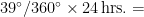) 2.6 hours for the distributed-parameter model and () 5.0 hours for the lumped-parameter model. (Actually, the plot overstates those values because it is based on a sinusoidal stimulus function; a half-wave-rectified sinusoid—which equinox diurnal radiation resembles more closely—would yield 2.4 and 4.3 hours, respectively.) As to seasonal lags, though, there’s no comparison. The distributed-parameter model’s seasonal lag, although admittedly low at 11 days, is of the right order of magnitude (at least if the location isn’t San Francisco). But, at less than a single day, the lumped-parameter model’s seasonal lag is way off. We are thereby justified in concluding that in at least this respect the lumped-parameter model is inferior.

Now, as the R code I used shows, the results above are highly dependent on the assumed material properties and on the two target frequency-response values the models are required to match. Moreover, to match those values I assumed a feedback value considerably more negative than popular estimates–as well as a thermal-conductivity value nearly two orders of magnitude higher than water’s (although ocean mixing may make the effective conductivity there quite a bit higher). When this model is made to match those targets, that is, it results in tautochrones that don’t look much like those in Mr. Eschenbach’s post. So there is plenty to criticize in at least this example of a distributed-parameter model.

But it’s also far from self-evident that the lumped-parameter models’ equations are always the more-relevant ones for studying climate lags. So we may occasionally want to try diffusion-based models instead of the lumped-parameter models to which we’re accustomed.

The Underlying R Code:

slabStepResponse <-function(z, k, rhoC, f, delta_t, N_h) {

# Finds the temperature response of a semi-infinite slab made of a

# thermally homogeneous, isotropic material that extends throughout z > 0 and

# leaves a free surface at the xy plane, where it receives incoming radiation

# whose power per unit area is uniform in x and y is a unit step as a

# function of time.

# Here:

# z is the depth at which the temperature is to be determined;

# k is the slab material’s thermal conductivity;

# rhoC is the product of the material’s density and its specific heat;

# f is the coefficient of net re-radiation (and/or conduction and/or

# convection) by which the slab loses power from the slab surface in

# in proportion to the surface’s temperature;

# delta_t is the time interval between instants at which the routine

# provides response values; and

# N_h is the number of response values to be determined.

#

# Rather than use thermal diffusivity “a” as an argument directly, the routine

# uses rhoC under the assumption that we can constrain the relationship

# between thermal conductivity and thermal diffusivity to values that are

# realistic for liquids and solids if we keep rhoC between 1.5 x 10^6

# and 4.5 x 10^6 J/K-m^3.

# (For water, rhoC = 4.186 x 10^6 and k = 0.58 W/m-K. However, cirulation no

# doubt makes the effective thermal conductivity at the oceans’ surfaces

# much higher than this.)

# Compute diffusivity from conductivity and specific heat:

a = k / rhoC;

# In the application to which we will apply this function, it is convenient for

# the time values to equal odd numbers times half the time step:

t = seq(1, N_h) * delta_t – delta_t / 2;

# Find the step response

u=1/f*(erfc(z/2/(a*t)^(1/2))-exp((f/k)*z+(f^2/k^2)*a*t)*erfc(z/2/(a*t)^(1/2)

+ f/k*(a*t)^(1/2)));

# Kludge to eliminate artifacts of computational limitations; unlikely to be

# robust to large parameter changes, so do a sanity check by plotting the

# step response for the intended parameter set:

u = u[!is.nan(u)]; # Lose the NaNs

u[1:max(1,length(u) – 20)] # Return the result without the ragged end

# Although the step response has a value of zero at t = 0, this

# routine’s output will start out non-zero, since its first value is the

# temperature at t = delta_t/2, not t = delta_t.

}

slabImpulseResponse <- function(z, k, rhoC, f, delta_t, N_h) {

# Since it is numerically awkward to evaluate the slab’s impulse response

# directly from its analytically determined value, we numerically

# differentiate its step response.

u = slabStepResponse(z, k, rhoC, f, delta_t, N_h)

M = length(u);

c(u[1], u[-1] – u[-M]);

}

slabResponse <- function(surfaceStimulus, z, k, rhoC, f, delta_t, N_h){

# Determines a semi-infinite slab’s response to surfaceStimulus.

# See slabStepResponse() for a description of the other arguments.

# First compute the slab’s impulse response:

u = slabImpulseResponse(z, k, rhoC, f, delta_t, N_h);

# Then return the convolution of the stimulus with the impulse response:

convolve(u, rev(surfaceStimulus), type = “o”)[1:length(surfaceStimulus)];

}

# The criterion we use here to decide whether the slab approach may in some

# way be superior to a simple single-pole approach whether the phase-shift

# behavior of the slab frequency response whose amplitude values for daily and

# annual frequencies match the earth’s matches the earth’s phase-shift behavior

# better than that of a single-pole model whose amplitudes do.

span <- function(F) max(F) – min(F)

lastPeriod <- function(F, omega, delta_t) F[(1 + length(F) – round(2 * pi / omega / delta_t)):length(F)]

slabFrequencyResponse <- function(z, k, rhoC, f, N_h, f_lo, f_hi, N_c, N_F, N_freq){

# This routine computes the frequency response of a slab.

# f_lo and f_hi define the frequency range over which the response is to

# be computed.

# N_c is the number of sine-wave cycles in the stimulus record to be used.

# The ratio of temperature to radiation is actually based on only a single

# cycle, but, since the response calculation in effect assumes zero stimulus

# before time -delta_t / 2, it was though that computing the response for

# several cycles before the one on which the ratio is based would tend to

# suppress transient-caused inaccuracy.

# N_F is the number of “samples” in the stimulus record.

# N_freq is the number of frequencies for which the response is to be computed

r = exp(log(f_hi / f_lo) / (N_freq – 1)); # ratio between successive frequency values

freq = f_lo * r^seq(0, N_freq – 1);

delta_t = N_c / freq / N_F; # Different delta_t’s for different frequencies

H = rep(0, N_freq);

phi = H;

for(i in 1:N_freq){

t = delta_t[i] * seq(0, N_F – 1);

omega = 2 * pi * freq[i];

# Create the stimulus:

F = sin(omega * t);

# Compute the time-domain response:

T = slabResponse(F, z, k, rhoC, f, delta_t[i], N_h);

# Throw away all but the last cycle

F = lastPeriod(F, omega, delta_t[i]);

T = lastPeriod(T, omega, delta_t[i]);

# Compute one amplitude value of the frequency response:

H[i] = span(T) / span(F);

# Create a quadrature signal:

t = lastPeriod(t, omega, delta_t[i]);

F_quad = sin(omega * t – pi / 2);

# Compute the phase angle by correlating the response

# with the in-phase and quadrature signals:

phi[i] = -atan(sum(F_quad * T) / sum(F * T)) * 180 / pi;

}

cbind(freq, H, phi);

}

# Now, to compute the frequency response, we assume some parameter values:

z = 0; # Depth at which the slab’s temperature response is to be determined

# Looking up material properties suggests that these values are in the right range:

k = 1.0 # Thermal conductivity

rhoC = 2e6 # Product of density and specific heat

# And the following value approximates what climate types call zero “feedback”:

f = 3 # coefficient of net surface-temperature-proportional surface heat loss

# By trial and error, however, I instead adopted these values:

k = 48;

f = 13;

# because they make the slab’s response amplitude match the following targets:

H_daily = 0.011 # My estimate of the mid-latitude response at frequency = 1 / day.

H_annual = 0.060 # My estimate of the mid-latitude response at frequency = 1 / year.

N_c = 16 # Number of oscillations the (sinusoidal) stimulus record is to span

N_F = 2048; # Number of “samples” in the (synthetic) stimulus record

N_h = N_F + 20; # Number of impulse-response values to be used in the convolution

# See slabStepResponse() kludge for origin of magic number 20.

N_freq = 27; # Number of frequency-response values to be generated

r = exp(log(365.2425) / (N_freq – 9)); # Frequency-step ratio

# Lowest and highest frequencies at which frequency response is to be evaluated

f_lo = r^(-4) / 365.2425 / 24 / 60 / 60; # Four values below once per year

f_hi = f_lo * r^(N_freq – 1); # Four

# Using those parameter values, compute the frequency response:

dummy = slabFrequencyResponse(z, k, rhoC, f, N_h, f_lo, f_hi, N_c, N_F, N_freq);

amplitude = dummy[ ,2];

amplRange = range(amplitude);

frequency = dummy[,1];

phaseAngle = dummy[ ,3];

cyclesPerYear = 365.2425 * 24 * 3600 * frequency;

freqRange = range(cyclesPerYear);

# Plot response amplitude:

plot(cyclesPerYear, amplitude, type = “l”, xlab = “Frequency, cycles/year”,

ylab = “Temp. Response, K-m^2 / W”, log = “xy”);

# Add lines to show the criterion values:

lines(c(1, 1), amplRange, lty = 2);

lines(c(365.2425, 365.2425), amplRange, lty = 2);

lines(freqRange, c(H_daily, H_daily), lty = 2);

lines(freqRange, c(H_annual, H_annual), lty = 2);

# Also by trial and error, I found these earth-response-matching values for a

# single-pole lumped-parameter model:

tau = 73046;

lambda = 0.05999;

singlePoleAmp = lambda /sqrt(1 + (2 * pi * frequency * tau)^2)

singlePolePhase = -atan(2 * pi * frequency * tau) * 180 / pi

# Plot that model’s response amplitude, too:

lines(cyclesPerYear, singlePoleAmp, col = “red”)

legend(150, 0.07, c(“Distributed”,”Lumped”), cex=0.8, col=c(“black”,”red”), lty = 1);

title(paste(“Distributed: f = “, f, “, k = “, k, “\nLumped: lambda = “, lambda, “, tau = “, tau, sep = “”));

# That should show that the distributed-parameter model varies much

# more graduall with frequency than the lumped-parameter model does

# Now make the same graphical comparison for the models’ phase-angle behavior:

plot(cyclesPerYear, phaseAngle, type = “l”, ylim = c(-90, 0),log = “x”);

lines(cyclesPerYear, singlePolePhase, col = “red”);

legend(150, 0, c(“Distributed”,”Lumped”), cex=0.8, col=c(“black”,”red”), lty =1);

title(paste(“Distributed: f = “, f, “, k = “, k, “\nLumped: lambda = “, lambda, “, tau = “, tau, sep = “”));

lines(c(1, 1), c(-95, 5), lty = 2);

lines(c(365.2425, 365.2425), c(-95, 5), lty = 2);

# What that should show is that the distributed model exhibits a much less

# significant variation in phase angle than the lumped-parameter model does.

# Whereas the lumped-parameter model suggests less than a day of seasonal lag

# but over five hours of (equinox) diurnal lag:

singlePolePhase[5] / 360 * 365.2425 # -0.8453802

singlePolePhase[22] / 360*24 # -5.023814

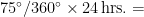
# the distributed-parameter model suggests an eleven-day seasonal lag (low

# but the right order of magnitude) and about two and a half hours

# of (equinox) diurnal lag (perhaps a little low):

phaseAngle[5] / 360 * 365.2425 # -10.93371

phaseAngle[22]/360*24 # -2.560662